a subdivision scheme for hexahedral meshes

A subdivision scheme for hexahedral meshes

Chandrajit Bajaj

Department of Computer Sciences, University of Texas

Scott Schaefer

Department of Computer Science, Rice University

Joe Warren

Department of Computer Science, Rice University

Guoliang Xu

State Key Laboratory of Scientific and Engineering Computing,

Chinese Academy of Sciences, Beijing

Keywords: subdivision, hexahedral, meshes, volume, generation

Abstract

In a landmark paper, Catmull and Clark described a simple generalization of the subdivision rules for bi-

cubic B-splines to arbitrary quadrilateral surface meshes. This subdivision scheme has become a main-

stay of surface modeling systems. Joy and MacCracken described a generalization of this surface scheme

to volume meshes. Unfortunately, little is known about the smoothness and regularity of this scheme due

to the complexity of the subdivision rules. This paper presents an alternative subdivision scheme for

hexahedral volume meshes that consists of a simple split and average algorithm. Along extraordinary

edges of the volume mesh, the scheme provably converges to a smooth limit volume. At extraordinary

vertices, the authors supply strong experimental evidence that the scheme also converges to a smooth

limit volume. The scheme automatically produces reasonable rules for non-manifold topology and can

easily be extended to incorporate boundaries and embedded creases expressed as Catmull-Clark surfaces

and B-spline curves.

1 Introduction

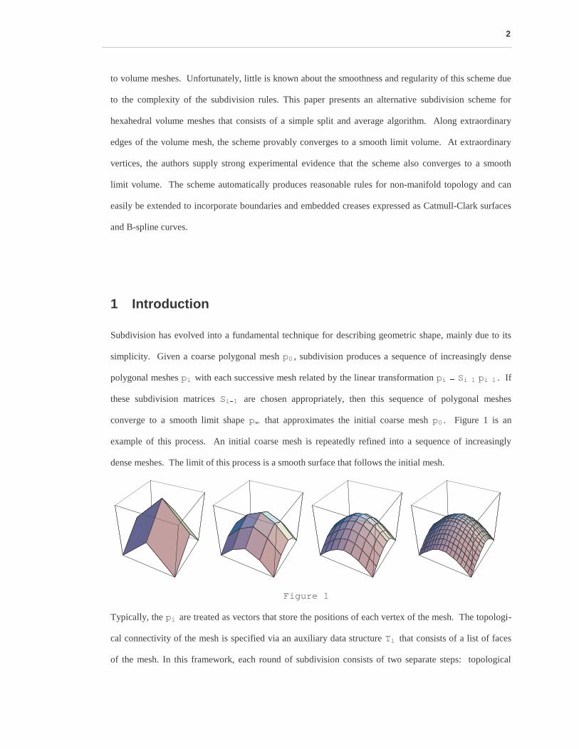
Subdivision has evolved into a fundamental technique for describing geometric shape, mainly due to its

simplicity. Given a coarse polygonal mesh p0 , subdivision produces a sequence of increasingly dense

polygonal meshes pi with each successive mesh related by the linear transformation pi� Si � 1 pi � 1 . If

these subdivision matrices Si � 1 are chosen appropriately, then this sequence of polygonal meshes

converge to a smooth limit shape p � that approximates the initial coarse mesh p0 . Figure 1 is an

example of this process. An initial coarse mesh is repeatedly refined into a sequence of increasingly

dense meshes. The limit of this process is a smooth surface that follows the initial mesh.

Fi gur e 1

Typically, the pi are treated as vectors that store the positions of each vertex of the mesh. The topologi-

cal connectivity of the mesh is specified via an auxiliary data structure Ti that consists of a list of faces

of the mesh. In this framework, each round of subdivision consists of two separate steps: topological

2

splitting of each face in Ti � 1 to produce Ti , then computing new vertex position pi via the subdivision

transformation Si � 1 pi � 1 . The beauty of this arrangement is that there are very simple rules for generat-

ing reasonable transformations Si � 1 (i.e. ones whose limit is well-behaved) directly from the topology

Ti � 1 . The example of figure 1 uses the subdivision rules for bi-cubic B-splines. Each quadrilateral is

split into four quadrilaterals. Each new vertex of pi is a convex combination of its nearby neighbors on

pi � 1 . One of three different combinations is used depending on whether the new vertex lies on a face,

edge or vertex of Ti � 1 .

Unfortunately, these rules only apply to quadrilateral meshes with tensor product topology (i.e. each

interior vertex is shared by four quadrilaterals). This restriction greatly reduces the applicability of these

rules. Standard shapes such as a sphere require meshes with non-tensor product topology. In a landmark

paper, Catmull and Clark [2] developed a generalization of the rules for bi-cubic B-splines that apply to

any type of quadrilateral mesh. In particular, they developed a rule for repositioning those vertices that

are shared by n quadrilaterals. This new rule was designed to produce smooth surfaces in the limit even

in the case of extraordinary vertices (i.e.n �4 ).

The development of this scheme ignited the growth of subdivision into a practical surface modeling tool.

Major corporations such as Pixar have adopted Catmull-Clark surfaces as their basic surface modeling

primitive. For volume modeling, the use of subdivision is still in its infancy. Joy and MacCracken [8]

introduced the first generalization of the rules for Catmull-Clark subdivision to volume meshes. Unfortu-

nately, the complexity of these rules makes analyzing the smoothness of the resulting volume scheme

very difficult and has in all likelihood hampered the use of the scheme in practice. In this paper, we

suggest an alternative set of subdivision rules that have a much simpler description in terms of splitting

and averaging. In addition, we provide a theoretical analysis that yields strong evidence that this new

scheme produces smooth volume meshes everywhere.

3

2 The scheme

To understand the new scheme, we first consider the subdivision rules for bi-cubic B-splines. Initially,

the bi-cubic rules were described in terms of topological splitting followed by vertex positioning. One

difficulty with this approach was the need for three types of positioning rules: one for each possible

topological position of a new vertex in Ti with respect to Ti � 1 (i.e. on a face of Ti � 1 , on an edge of

Ti � 1 , at a vertex of Ti � 1 ). One way to avoid this problem is to recast the bi-cubic rules into a slightly

different framework.

The geometric positioning rules embodied by the subdivision Si � 1 can be factored into two separate

transformations: bi-linear subdivision followed by a simple averaging operation. Figure 2 illustrates this

factorization for the first step of figure 1. A coarse mesh is first split using bi-linear subdivision. The

resulting mesh is then smoothed using a simple averaging operator supported over the nearby neighbors

of each vertex.

Fi gur e 2

There are two superficial advantages of this approach. First, bi-linear subdivision can be carried out

during topological splitting. Second, the averaging operator for tensor product meshes employs only a

single type of averaging rule. Similarly, the rule for tri-cubic subdivision can be factored into tri-linear

subdivision followed by averaging. The true advantage of this decomposition is that the problem of

developing a variant of the tri-cubic rule for arbitrary hexahedral meshes can be focused solely on the

averaging operation. This approach allows us to develop a single, simple averaging rule for arbitrary

4

meshes (as opposed to the four required under the Joy and MacCracken approach). Our task is to

develop a generalization of this averaging rule that reproduces the tensor product rule on tensor product

meshes and yields smooth limit volumes for arbitrary hexahedral meshes. This generalization, developed

in 2D by Morin et al. [10], Zorin and Schröder [20] and Stam [15] simultaneously , is remarkably simple.

2.1 Multi-linear subdivision

Before proceeding to the problem of averaging, we consider the problem of implementing multi-linear

subdivision. At first glance, this might appear to be an imposing task. However, with the correct choice

of data structures, implementing multi-linear subdivision is straightforward. (Note that we consider the

general d -dimensional case since the three dimensional solution allows for little simplification.) Essen-

tially, multi-linear subdivision consist of splitting a topological d -cube into 2d subcubes and positioning

the new vertices using multi-linear interpolation. To implement the topological split, we must first settle

on a representation for the topology of a d -dimensional cube (a d -cube). We suggest a simple, recur-

sive representation with a 0 -cube consisting of a vertex index and a d -cube (d � 0 ) consisting of a list

of two �d � 1 � -cubes. For example, a square consists of a list of two line segments and a cube consist

of a list of two squares. Given this representation, an algorithm for splitting a d -cube C into its 2d

subcubes is as follow:

Given a d -cube C, recursively compute the multi-linear subdivision of two �d � 1 � -cubes comprising C

and call the two resulting lists of 2d � 1 (d � 1 )-cubes t op and bot t om, respectively. t op and

bot t om are splits of the "top" and "bottom" faces of C. Next, use linear interpolation to compute a list

of 2d � 1 (d � 1 )-cubes called mi ddl e that lie halfway between t op and bot t om. Finally, return 2d � 1

d -cubes from corresponding pairs of cubes in t op and mi ddl e and 2d � 1 d-cubes from corresponding

pairs of cubes in mi ddl e and bot t om.

Given this topological representation for a single d -cube, the topology Ti for a mesh of d -cubes is

simply a list of such d -cubes. To ensure topological consistency of this representation, each new vertex

that is common to several subcubes must use the same index for each subcube. To maintain these

5

indices, we suggest using a hash table. The hash table can be indexed by the smallest d-cube on the

coarse mesh that contains each vertex. For instance, a vertex inserted on an edge would be indexed by

the two vertices that make up that edge.

2.2 Cell averaging

The key to finding a suitable averaging operator for non-tensor product meshes is to understand the

structure of the averaging operator in the tensor product case. In the univariate case, the subdivision

rules for cubic B-splines can be expressed as linear subdivision followed by averaging with the mask

� 1�� 4

1�� 2

1�� 4� . Specifically, the subdivision matrix Sk � 1 can be decomposed as follows:

�

�

��

. . . . . . .

. 1� � � �8

3� � � �4

1� � � �8

0 0 .

. 0 1� � � �2

1� � � �2

0 0 .

. 0 1� � � �8

3� � � �4

1� � � �8

0 .

. 0 0 1� � � �2

1� � � �2

0 .

. 0 0 1� � � �8

3� � � �4

1� � � �8

.

. . . . . . .

�

�

��

�

�

�

��

. . . . . . .

. 1� � � �4

1� � � �2

1� � � �4

0 0 .

. 0 1� � � �4

1� � � �2

1� � � �4

0 .

. 0 0 1� � � �4

1� � � �2

1� � � �4

.

. . . . . . .

�

�

��

.

�

�

��

. . . . .

. 1 0 0 .

. 1� � � �2

1� � � �2

0 .

. 0 1 0 .

. 0 1� � � �2

1� � � �2

.

. 0 0 1 .

. . . . .

�

�

��

.

Note that application of the mask � 1�� 4

1�� 2

1�� 4� has a simple geometric interpretation: reposition a

vertex at the midpoint of the midpoints of the two segments that contain the vertex. In the bivariate case,

bi-cubic subdivision is equivalent to bi-linear subdivision followed by averaging with the tensor product

of the univariate mask with itself. Plotted in 2D, the coefficients of this averaging mask have the form

�

�

��

1��

161�� 8

1��

161�� 8

1�� 4

1�� 8

1��

161�� 8

1��

16

�

�

��. Note that this mask can be decomposed into the sum of four submasks,

�

�

��

1� � � � � �16

1� � � �8

1� � � � � �

161� � � �8

1� � � �4

1� � � �8

1� � � � � �16

1� � � �8

1� � � � � �

16

�

�

��

1� � � �

4

�

�

��

�

�

��

0 0 01� � � �4

1� � � �4

0

1� � � �4

1� � � �4

0

�

�

��

�

�

��

0 0 0

0 1� � � �4

1� � � �4

0 1� � � �4

1� � � �4

�

�

��

�

�

��

0 1� � � �4

1� � � �4

0 1� � � �4

1� � � �4

0 0 0

�

�

��

�

�

��

1� � � �4

1� � � �4

0

1� � � �4

1� � � �4

0

0 0 0

�

�

��

�

�

��.

This mask has a geometric interpretation analogous to the univariate case: reposition a vertex at the

centroid of the centroids of the four quadrilaterals that contain the vertex. The averaging mask for

tri-cubic B-splines (the tensor of the mask � 1� � �4

1�� 2

1� � �4� with itself three times) can be expressed

6

decomposed in a similar manner. Again, this mask has a geometric interpretation analogous to the

univariate case: reposition a vertex at the centroid of the centroids of the eight hexahedra that contain the

vertex. These geometric interpretations of the tensor product rules lead to our general rule for smoothing

a mesh of topological d -cubes,

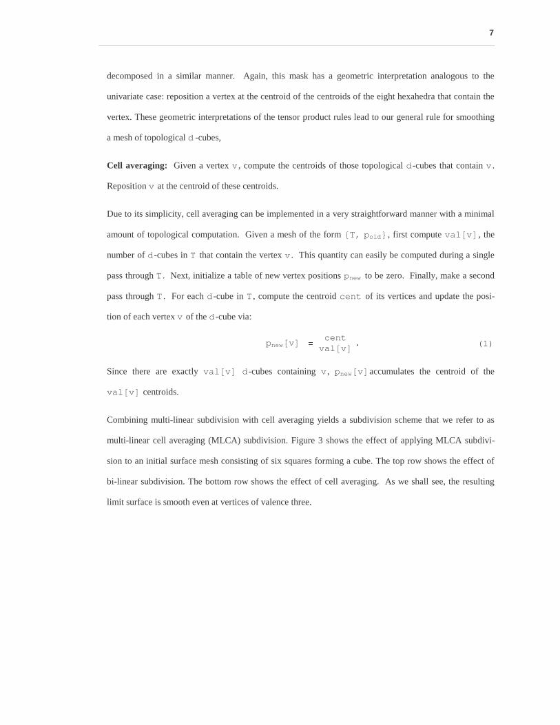
Cell averaging: Given a vertex v , compute the centroids of those topological d -cubes that contain v .

Reposition v at the centroid of these centroids.

Due to its simplicity, cell averaging can be implemented in a very straightforward manner with a minimal

amount of topological computation. Given a mesh of the form T, pol d , first compute val � v � , the

number of d -cubes in T that contain the vertex v . This quantity can easily be computed during a single

pass through T . Next, initialize a table of new vertex positions pnew to be zero. Finally, make a second

pass through T . For each d -cube in T , compute the centroid cent of its vertices and update the posi-

tion of each vertex v of the d -cube via:

( 1)pnew� v � � �cent

��

val � v � .

Since there are exactly val � v � d -cubes containing v , pnew� v � accumulates the centroid of the

val � v � centroids.

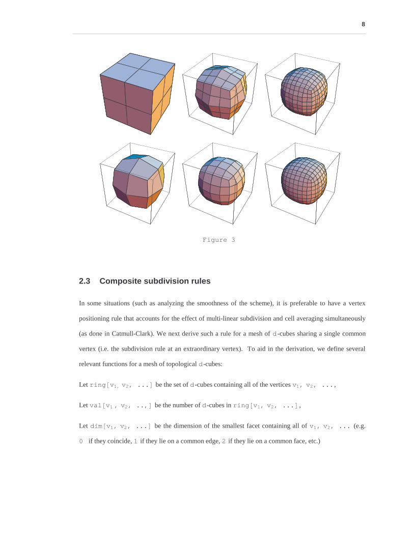
Combining multi-linear subdivision with cell averaging yields a subdivision scheme that we refer to as

multi-linear cell averaging (MLCA) subdivision. Figure 3 shows the effect of applying MLCA subdivi-

sion to an initial surface mesh consisting of six squares forming a cube. The top row shows the effect of

bi-linear subdivision. The bottom row shows the effect of cell averaging. As we shall see, the resulting

limit surface is smooth even at vertices of valence three.

7

Fi gur e 3

2.3 Composite subdivision rules

In some situations (such as analyzing the smoothness of the scheme), it is preferable to have a vertex

positioning rule that accounts for the effect of multi-linear subdivision and cell averaging simultaneously

(as done in Catmull-Clark). We next derive such a rule for a mesh of d -cubes sharing a single common

vertex (i.e. the subdivision rule at an extraordinary vertex). To aid in the derivation, we define several

relevant functions for a mesh of topological d -cubes:

Let r i ng � v1, v2, . . . � be the set of d -cubes containing all of the vertices v1, v2, . . . ,

Let val � v1 , v2, . . , � be the number of d -cubes in r i ng � v1, v2, . . . � ,

Let di m� v1, v2, . . . � be the dimension of the smallest facet containing all of v1, v2, . . . (e.g.

0 if they coincide, 1 if they lie on a common edge, 2 if they lie on a common face, etc.)

8

Given a coarse (old) Tol d, pol d , let Tnew, pnew be the fine (new) produced by MLCA subdivi-

sion. If v is a vertex of the old , then its position in the new is a weighted sum of the vertices u in

r i ng � v � on the old . In particular, we claim that the weight associated with u has the form:

( 2)1

��

4d val � v � 3d � di m� u, v � val � u, v �

For a one-dimensional curve (d � 1 ), val � v � is two for all vertices. Therefore, by equation 2, the

subdivision at vertex of Tol d has the form 31 � 1 � 1��

41 2, 31 � 0 � 2��

41 2, 31 � 1 � 1��

41 2� which is equal to

� 1�� 8

, 3�� 4

, 1�� 8� . In the surface case (d � 2 ), the subdivision rule at an extraordinary vertex of valence

n has the weights shown in figure 4. One interesting feature of the equation 2 is that the weight assigned

to the central vertex v by this rule is always � 3�� 4� d since val � v � � val � v, v � and

di m� v, v � � 0 .

Fi gur e 4

9� � � � � � �

163

� � � � � � � �

8 n

3� � � � � � � �

8 n3

� � � � � � � �

8 n

3� � � � � � � �

8 n3

� � � � � � � �

8 n

1��

16 n

1� � � � � � � � � � �

16 n

1� � � � � � � � � � �

16 n

1� � � � � � � � � � �

16 n

1��

16 n

We conclude this section by proving the correctness of equation 2. To this end, let C be a cell of Tnew

containing v and whose parent also contains u . After multi-linear subdivision, but prior to cell averag-

ing, the vertices of C involve weighted combinations of u due to repeated linear interpolation. If u and

v share a facet of dimension di m� u, v � in Tol d , then these weights appear on a complementary sub-

facet of C of dimension �d � di m� u, v � � . The sum of these weights in u is given by the expression

9

( 3)�i � 0

d � di m� u, v �� d � di m� u, v �

i� 2i � d.

where � ab� is the binomial coefficient a

��

b� �a � b � � .This expression can be simplified via Mathematica to

2 � d 3d � di m� u, v � . Thus, the total contribution of u to the centroid of C during cell averaging is

2 � d 3d � di m� u, v � divided by the number of vertices in the cell 2d . Thus, the total contribution of u to the

new position of v from the cell C is 3d � di m� u, v ��

4d val � v � . Since there are val � u, v � cells that contain u and

v , the total contribution over all cells must be as in equation 2. Since both multi-linear subdivision and

cell averaging reproduce constants, the weights of equation 2 must form a partition of unity, i.e.

( 4)�u � r i ng � v �

3d � di m� u, v � val � u, v � � 4d val � v � .

3 Extensions

3.1 Non-manifold meshes

One particular advantage of MLCA subdivision is that it makes no restrictions on the local topology of

the mesh. In particular, the scheme can be applied without change to meshes with non-manifold topol-

ogy. In the univariate case, non-manifold topology gives rise to curve networks with n � 2 segments

meeting at a vertex. The vertex positioning rule at such a non-manifold vertex takes 3�� 4

of the original

vertex plus 1��

4 n times each of its n neighbors. This rule is very similar to the variational rule for curve

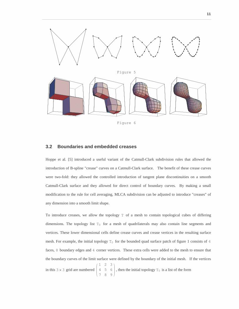
networks developed in Warren and Weimer [18]. Figure 5 show an example of MLCA averaging

subdivision applied to an butterfly shaped curve network. Figure 6 shows an example of an MLCA

subdivision applied to a quadrilateral mesh consisting of 12 squares. The final surface mesh inherits the

non-manifold curve present in the initial mesh.

10

Fi gur e 5

Fi gur e 6

3.2 Boundaries and embedded creases

Hoppe et al. [5] introduced a useful variant of the Catmull-Clark subdivision rules that allowed the

introduction of B-spline "crease" curves on a Catmull-Clark surface. The benefit of these crease curves

were two-fold: they allowed the controlled introduction of tangent plane discontinuities on a smooth

Catmull-Clark surface and they allowed for direct control of boundary curves. By making a small

modification to the rule for cell averaging, MLCA subdivision can be adjusted to introduce "creases" of

any dimension into a smooth limit shape.

To introduce creases, we allow the topology T of a mesh to contain topological cubes of differing

dimensions. The topology list T0 for a mesh of quadrilaterals may also contain line segments and

vertices. These lower dimensional cells define crease curves and crease vertices in the resulting surface

mesh. For example, the initial topology T0 for the bounded quad surface patch of figure 1 consists of 4

faces, 8 boundary edges and 4 corner vertices. These extra cells were added to the mesh to ensure that

the boundary curves of the limit surface were defined by the boundary of the initial mesh. If the vertices

in this 3 � 3 grid are numbered �

�

��1 2 34 5 6

7 8 9

�

�

�� , then the initial topology T0 is a list of the form

11

1, 2, 5, 4 , 4, 5, 8, 7 , 2, 3, 6, 5 , 5, 6, 9, 8 , 1, 4 , 4, 7 , 1, 2 , 2, 3 , 3, 6 , 6, 9 , 7, 8 , 8, 9 ,

1 , 3 , 7 , 9 .

Given this new representation, multi-linear subdivision is performed as usual with each d -cube split into

2d subcubes. However, cell averaging is adjusted as follows: for each vertex v , we compute di m� v � ,

the dimension of the lowest dimension cell in T that contains v . In the example above, di m� v � has the

values

v : 1 2 3 4 5 6 7 8 9

di m� v � : 0 1 0 1 2 1 0 1 0

di m� v � as well as val � v � (now the number of cells containing v of dimension di m� v � ) can be

computed in a single pass through T . Given these two quantities, the averaging rule of equation 1 can be

reused with the following adjustment:

Cell averaging with creases : Given a vertex v , compute the centroids of those cells of dimension

di m� v � that contain v . Reposition v at the centroid of these centroids.

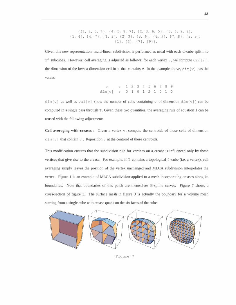
This modification ensures that the subdivision rule for vertices on a crease is influenced only by those

vertices that give rise to the crease. For example, if T contains a topological 0 -cube (i.e. a vertex), cell

averaging simply leaves the position of the vertex unchanged and MLCA subdivision interpolates the

vertex. Figure 1 is an example of MLCA subdivision applied to a mesh incorporating creases along its

boundaries. Note that boundaries of this patch are themselves B-spline curves. Figure 7 shows a

cross-section of figure 3. The surface mesh in figure 3 is actually the boundary for a volume mesh

starting from a single cube with crease quads on the six faces of the cube.

Fi gur e 7

12

Figure 8 shows an example of a volume mesh with different types of creases. The "A" is constructed out

of cubes and the surface is covered with quads. The bottom of the "A's" legs have crease curves around

them as does the hole in the center. In the wireframe picture it is possible to see the cubes that make up

the "A" as it is subdivided. This figure was produced with the method in [10] where tensions are

attached to the edges of the mesh. This allows the mesh to converge to circles on the bottom and in the

center. Figure 9 shows a torus that uses tensions as well to reproduce circles. The original figure is

made up of four cubes and sixteen quads on its surface. Again, the wireframe shows the cubes that make

up the figure being subdivided.

Fi gur e 8

Fi gur e 9

13

Figure 10 shows two examples of objects modeled using MLCA subdivision. Each mesh is a volume

mesh whose boundary is made to conform to the shape of a ring and an axe, respectively, using crease

surface, crease edges and crease vertices.

Fi gur e 10

A ring and an axe modeled using MLCA subdivision with creases.

Finally, we note that the ability to define smooth volume meshes with embedded crease surface should be

particularly useful. 3D application such as geological modeling require precise representation of embed-

ded faults and fractures. We intend to pursue applications of MLCA subdivision in this area.

3.3 Non-hexahedral initial meshes

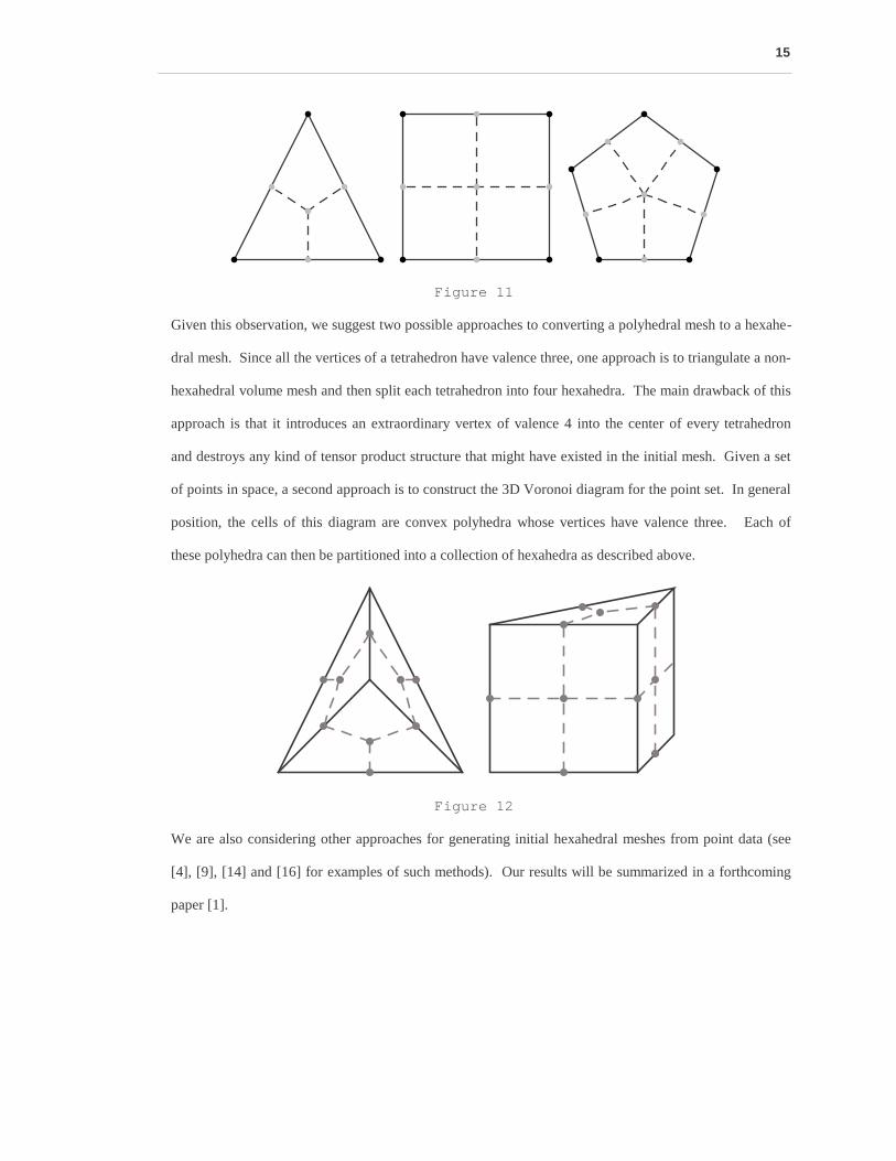
Any polygonal surface mesh can be converted into a quadrilateral mesh by splitting each face n -gon into

n quadrilateral faces. Each of these n quadrilaterals consist of a vertex, the midpoints of its two incident

edges and the centroid of the polygon. Figure 11 shows three examples of this split. Ideally, a similar

method would allow one to split any convex polyhedron into a mesh of hexahedra. Unfortunately, such a

split is possible only for those polyhedra for which all vertices have valence three. Given such a polyhe-

dra with n vertices, it can be split into n hexahedra where each hexahedra consists of a vertex, 3 adja-

cent edge midpoints, 3 adjacent face centers and the centroid of the original polyhedron. Note that the

split on the faces of the polyhedron is exactly the 2D split for a polygon. Figure 12 shows two examples

of this 3D split for a tetrahedron and a triangular prism.

14

Fi gur e 11

Given this observation, we suggest two possible approaches to converting a polyhedral mesh to a hexahe-

dral mesh. Since all the vertices of a tetrahedron have valence three, one approach is to triangulate a non-

hexahedral volume mesh and then split each tetrahedron into four hexahedra. The main drawback of this

approach is that it introduces an extraordinary vertex of valence 4 into the center of every tetrahedron

and destroys any kind of tensor product structure that might have existed in the initial mesh. Given a set

of points in space, a second approach is to construct the 3D Voronoi diagram for the point set. In general

position, the cells of this diagram are convex polyhedra whose vertices have valence three. Each of

these polyhedra can then be partitioned into a collection of hexahedra as described above.

Fi gur e 12

We are also considering other approaches for generating initial hexahedral meshes from point data (see

[4], [9], [14] and [16] for examples of such methods). Our results will be summarized in a forthcoming

paper [1].

15

4 Smoothness analysis

The MLCA subdivision scheme is applicable to meshes of both quadrilaterals in two dimensions and

meshes of hexahedra in three dimensions. In this section, we analyze the smoothness of MLCA scheme

in each case. In two dimension, we show that the scheme produces limit surfaces that are smooth

everywhere. In three dimension, we prove that MLCA subdivision converges to a smooth limit volume

along extraordinary edges of the mesh. At extraordinary vertices of the 3D mesh, we examine the

characteristic map for MLCA subdivision and provide strong evidence that MLCA subdivision most

likely converges to smooth limit volume at these vertices. The key to this analysis is the spectral

technique described in Reif [13], Prautzsch [12], Peters and Reif [11] and Warren [17].

4.1 The surface case

For quadrilateral meshes, topological subdivision produces quadrilateral meshes that are locally tensor

product almost everywhere. In particular, the meshes are locally tensor product everywhere except at

extraordinary points (i.e. those vertices of the original mesh whose valence is not four). Since MLCA

subdivision was designed to reproduce the subdivision rule for bi-cubic B-splines on tensor product

meshes, the limit surfaces produced by the scheme are C2 everywhere except at these extraordinary

points. Thus, our task is to determine the smoothness of MLCA subdivision at an extraordinary vertices.

Luckily, much of the analysis has been done in previous work by Reif and Peters [11] on the smoothness

of Catmull-Clark subdivision at an extraordinary vertex v .

16

Consider an extraordinary point v shared by n quadrilaterals. In the neighborhood of v , repeated

topological subdivision yields a topological mesh T consisting of n quadrants of a tensor product mesh

surrounding v (see figure 13). In this framework, the behavior of the subdivision scheme at v is charac-

terized by the spectral structure of the subdivision matrix S associated with T . For a valence five

extraordinary vertex v , the matrix S (restricted to r i ng � v � ) has the form:

( 5)

�

�

��

1 � na 6 a 6 a 6 a 6 a 6 a a a a a a3�� 8

3�� 8

1��

160 0 1��

161��

160 0 0 1��

163�� 8

1��

163�� 8

1� ��

160 0 1��

161��

160 0 0

3�� 8

0 1��

163�� 8

1��

160 0 1��

161��

160 0

3�� 8

0 0 1� ��

163�� 8

1��

160 0 1��

161��

160

3�� 8

1��

160 0 1��

163� � �8

0 0 0 1��

161��

161�� 4

1�� 4

1�� 4

0 0 0 1�� 4

0 0 0 0

1�� 4

0 1�� 4

1�� 4

0 0 0 1�� 4

0 0 0

1�� 4

0 0 1�� 4

1�� 4

0 0 0 1�� 4

0 0

1�� 4

0 0 0 1�� 4

1� � �4

0 0 0 1�� 4

0

1�� 4

1�� 4

0 0 0 1� � �4

0 0 0 0 1�� 4

�

�

��

Note that we have not completely specified the position rule at the extraordinary vertex. The variable a

is free and can be chosen as a function of n .

If the eigenvalues �

i of S and their corresponding eigenvectors z i are indexed in order of decreasing

magnitude, a necessary condition for building a subdivision scheme with linearly independent scaling

functions that is smooth at an extraordinary vertex v is that these eigenvalues must satisfy

1 ��

0 � � �1 � � � �

2 � � � �3 � � . . . (see [12], [21]) . Based on the block circulant structure of S,

the eigenvalues and eigenvectors of S can be computed directly using the discrete Fourier transform. All

but two of the eigenvalues of S (and their corresponding eigenvectors) are independent of the choice of

a . The remaining two eigenvalues (and their corresponding eigenvectors) depend on the choice of a

and are eigenvalues of the reduced matrix

( 6)

�

�

��

1 � 7 n a 6 n a n a3�� 8

1�� 2

1�� 8

1�� 4

1�� 2

1�� 4

�

�

��.

17

Now, Catmull-Clark suggests a vertex rule with a � 1� ��

4 n2 . Using some basic calculus, Reif and Peters

[11] show that the eigenvalues of the resulting S are real and satisfy 1 ��

1 ��

2 � ��

3 … where

�2 � 1��

4. On the other hand, the subdivision matrix S for MLCA subdivision has a vertex rule with

a � 1��

16 n. For this choice of a , the two eigenvalues of the reduced matrix in equation 6 are 1��

4 and 1��

16.

Since the remaining eigenvalues of S are unchanged, the spectrum of S continues to satisfy

1 ��

1 ��

2 ��

3 … for MLCA subdivision.

Unfortunately, this condition alone is not sufficient to guarantee that the scheme is smooth at the extraor-

dinary vertex v . For schemes with a spectrum of the form �

0 � 1 � � �1 � � � �

2 � � …, the eigenvec-

tors z1 and z2 corresponding to the subdominant eigenvalues �

1 and �

2 determine whether the limit

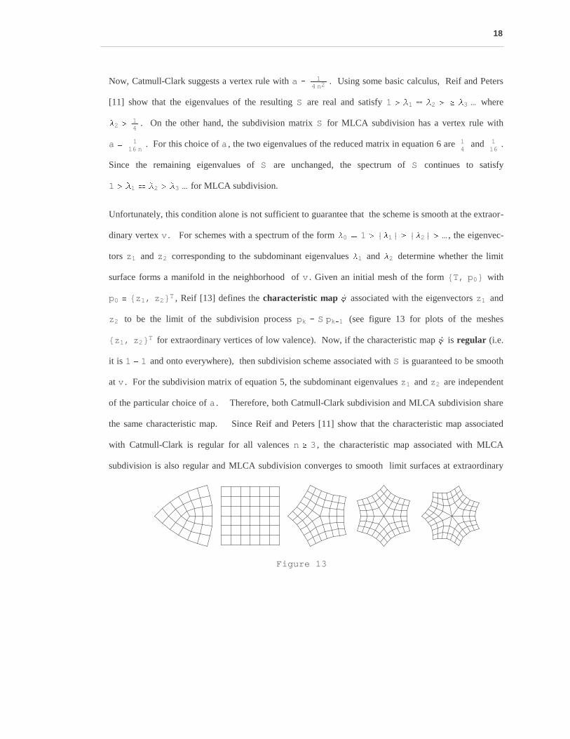
surface forms a manifold in the neighborhood of v . Given an initial mesh of the form T, p0 with

p0� z1, z2 T , Reif [13] defines the character istic map � associated with the eigenvectors z1 and

z2 to be the limit of the subdivision process pk� S pk � 1 (see figure 13 for plots of the meshes

z1, z2 T for extraordinary vertices of low valence). Now, if the characteristic map � is regular (i.e.

it is 1 � 1 and onto everywhere), then subdivision scheme associated with S is guaranteed to be smooth

at v . For the subdivision matrix of equation 5, the subdominant eigenvalues z1 and z2 are independent

of the particular choice of a . Therefore, both Catmull-Clark subdivision and MLCA subdivision share

the same characteristic map. Since Reif and Peters [11] show that the characteristic map associated

with Catmull-Clark is regular for all valences n � 3 , the characteristic map associated with MLCA

subdivision is also regular and MLCA subdivision converges to smooth limit surfaces at extraordinary

Fi gur e 13

18

4.2 The volume case

To analyze the smoothness of MLCA subdivision on hexahedral meshes, we first consider the effect of

topological subdivision on a hexahedral mesh. Repeated subdivision of a single hexahedron produces a

tensor product volume mesh on the interior of the hexahedra. This tensor product structure extends

uniformly across the faces of the hexahedra to face adjacent hexahedra. Since MLCA subdivision

reproduces the subdivision rule for tri-cubic B-splines on tensor product meshes, the limiting volumes

are C2 on both the interiors of the hexahedra and the interiors of their faces.

For n hexahedra sharing a common edge, repeated topological subdivision yields a volume mesh whose

topology is the tensor product of a uniform quad mesh surrounding an extraordinary vertex of a valence

n extraordinary point and a curve mesh. Figure 14 shows local examples of such meshes for n � 3 and

n � 5 . Using equation 2, one can verify that the subdivision rules produced by MLCA along this

"extraordinary" edge are the tensor product of the bivariate MLCA rule for a valence n vertex and the

univariate rule for cubic B-splines. Since these rules deliver C1 surfaces and C2 curves respectively,

the tensor product rules produces C1 volumes. Note that volume scheme of Joy and MacCracken does

not have this tensor product property. As a result, analyzing the smoothness of Joy and MacCracken

scheme along extraordinary edges appears to be impossible with current analysis techniques.

Fi gur e 14

All that remains is to analyze the smoothness of MLCA subdivision at extraordinary vertices of the

original mesh. Given a vertex v of the original hexahedral mesh, repeated topological subdivision

produces an infinite topological mesh T that is invariant under topological subdivision and whose

19

structure is determined by r i ng � v � . As in the two-dimensional case, the spectral structure of the

subdivision matrix S associated with this mesh T governs the behavior of the subdivision scheme at v .

In particular, we believe that conditions on the subdominant eigenvalues and eigenvectors of S similar to

those given by Reif in [13] are the key to analyzing the smoothness of this scheme at an extraordinary

vertex. The crux of this analysis would be constructing a three-dimensional analog of the characteristic

map based on the eigenvectors z1 , z2 , and z3 associated with the subdominant eigenvalues �

1 , �

2 and

�3 , respectively. However, we leave a precise characterization of these conditions and a proof of their

correctness for future work.

One obstacle to this type of smoothness analysis in the three-dimensional case is that the topological

mesh T lacks the rotational symmetries that made it possible to use the discrete Fourier transform to

compute the spectral structure of S in two dimensions. In general, the spectral structure of S depends on

the topological structure of r i ng � v � in a way that appears to defy symbolic computation. Instead, one

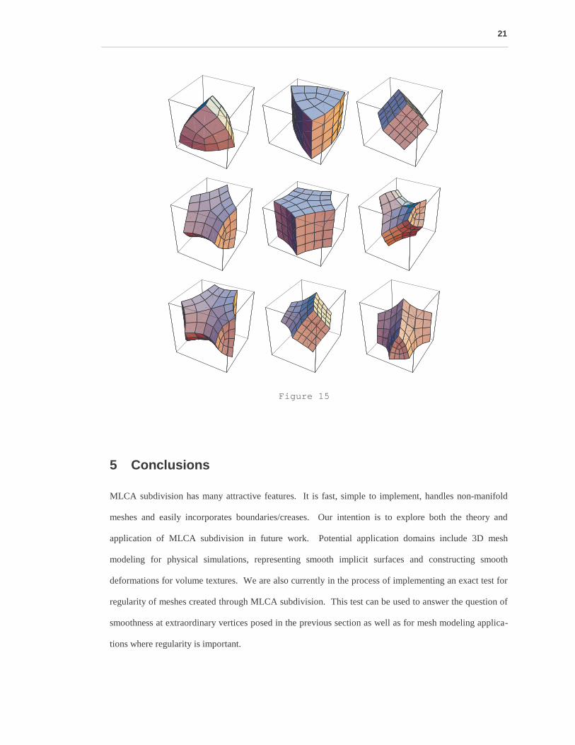
possibility is to use a brute force approach and simply enumerate possible topologies for r i ng � v � . For

each distinct topology, we compute the eigenvalues and eigenvectors of S restricted to the two-ring of

v . Figure 15 shows plots of the mesh defined by the subdominant eigenvectors of S (i.e. the charac-

terisitc map) for nine distinct low valence topologies (all configurations for which the extraordinary

vertex v has 7 or few edge adjacent neighbors). Based on a visual examination of these meshes, their

associated characteristic maps appear to be regular. However, developing a rigorous, computational

method for testing the regularity of these meshes is also the subject of future work.

20

Fi gur e 15

5 Conclusions

MLCA subdivision has many attractive features. It is fast, simple to implement, handles non-manifold

meshes and easily incorporates boundaries/creases. Our intention is to explore both the theory and

application of MLCA subdivision in future work. Potential application domains include 3D mesh

modeling for physical simulations, representing smooth implicit surfaces and constructing smooth

deformations for volume textures. We are also currently in the process of implementing an exact test for

regularity of meshes created through MLCA subdivision. This test can be used to answer the question of

smoothness at extraordinary vertices posed in the previous section as well as for mesh modeling applica-

tions where regularity is important.

21

6 References

[1] Bajaj, C., Warren, J. and Xu, G.: Adaptive Hexahedral Finite Element Meshing of Solids with

Embedded Particles, manuscript, 2001.

[2] Catmull, E. and Clark, J.: Recursively generated B-spline surfaces on arbitrary topological meshes.

Computer-Aided Design, Vol 16, no. 6, pp. 350—355, 1978.

[3] Chaikin, G.: An Algorithm for High Speed Curve Generation. Computer Graphics and Image

Processing, 3, pp. 346-349, 1974.

[4] Eppstein, D.: Linear Complexity Hexahedral Mesh Generation, Proceedings of the Twelfth Annual

Symposiam on Computational Geometry, pp. 58—67, 1996.

[5] Hoppe, Hugues and DeRose, Tony and Duchamp, Tom and Halstead, Mark and Jin, Hubert and

McDonald, John and Schweitzer, Jean and Stuetzle, Werner: Piecewise smooth surface reconstruction.

In SIGGRAPH94 proceedings, annual conference series, ACM press, pp. 295—302, 1994.

[6] Lane, J. M. and Riesenfeld, R. F.: A theoretical development for the computer generation and

display of piecewise polynomial functions. Transactions on Pattern Analysis and Machine Intelligence,

vol. 2, no. 1, pp. 35—46, 1980.

[7] Loop, Charles T.: Smooth subdivision surfaces based on triangles. Master's Thesis, Department of

Mathematics, University of Utah, August 1987.

[8] MacCracken, R. and Joy, K.: Free-form deformations of soid primitives with constraints.

Proceedings of SIGGRAPH 1996, Computer Graphics Proceedings, Annual Conference Series, pp.

181—188 (July 1996). ACM Press / ACM SIGGRAPH / Addison Wesley Longman. 1996.

[9] Mitchell, S.: Hexahedral mesh generation via the dual, 11th ACM Symposiam on Computational

Geometry, pp. C4—C5, 1995.

22

[10] Morin, Géraldine, Warren, Joe and Weimer, Henrik: A Subdivision Scheme for Surfaces of

Revolution. Computer-Aided Geometric Design, Vol. 18, pp. 483-502, 2001.

[11] Peters, Jorg and Reif, Ulrich: Analysis of Generalized B-Spline Subdivision Algorithms. SIAM

Journal of Numerical Analysis 35, pp. 728—748, 1998.

[12] Prautzsch, Hartmut: Smoothness of subdivision surfaces at extraordinary points. Advances in

Computational Mathematics, 9, pp. 377—389, 1998.

[13] Reif, Ulrich: A unified approach to subdivision algorithms near extraordinary points. Computer-

Aided Geometric Design, Vol 12, pp. 153—174, 1995.

[14] Schneiders, R. and Bunten, R., Automatic Generation of Hexahedral Finite Element Meshes,

Computer-Aided Geometric Design, Vol 12, pp. 693—707, 1995.

[15] Stam, Jos: On subdivision schemes generalizing B-splines surfaces of arbitrary degree. Computer-

Aided Geometric Design, Vol 18, pp. 383-386, 2001.

[16] Tautges, T., Blacker, T. and Mitchell, S.: The Whisker Weaving Algorithm: A Connectivity-Based

Method for Constructing All-Hexahedral Finite Element Meshes, International Journal for Numerical

Methods in Engineering, vol. 39, pp. 3327-3349, 1996.

[17] Warren, Joe: Subdivision Methods for Geometric Design, Manuscript available online at

http://www.cs.rice.edu/~jwarren/, 1995.

[18] Weimer, Henrik and Warren, Joe: Subdivision Schemes for Thin Plate Splines. Proceedings of

Eurographics 1998, Computer Graphics Forum, Vol 17, no. 3, pp. 303—313 & 392, 1998.

[19] Zorin, Denis, Schröder, Peter and Sweldens, Wim: Interpolating subdivision for meshes with

arbitrary topology. In SIGGRAPH96 proceedings, annual conference series, ACM Press, pp.

189—192, 1996.

[20] Zorin, Denis and Schröder, Peter: A unified framework for primal/dual quadrilateral subdivision

schemes. Computer-Aided Geometric Design, Vol 18, pp. 483-502, 2001.

23

[21] Zorin, Denis: Smoothness of Subdivision on Irregular Meshes. Constructive Approximation, Vol

16, no. 3, pp. 359—397, 2000.

24

a subdivision scheme for hexahedral meshes

Documents