A Study on the Design Optimization of an AUV by Using Computational Fluid Dynamic Analysis

Taehwan Joung*, Karl Sammut*, Fangpo He*, and Seung-Keon Lee**

*School of Computer Science, Engineering and Mathematics, Faculty of Science & Engineering, Flinders University, Adelaide, Australia **Department of Naval Architecture and Ocean Engineering, Pusan National University, Busan, Korea

ABSTRACT Autonomous Underwater Vehicles (AUV's) provide an important means for collecting detailed scientific information from the ocean depths. The hull resistance of an AUV is an important factor in determining the power requirements and range of the vehicle. This paper describes a design method using Computational Fluid Dynamics (CFD) for determining the hull resistance of an AUV under development. The CFD results reveal the distribution of hydrodynamic values (velocity, pressure, etc.) of the AUV with a ducted propeller. The optimization of the AUV hull profile for reducing the total resistance is also discussed in this paper. This paper demonstrates that shape optimization in conceptual design is possible by using a commercial CFD package. The optimum designs to minimize the drag force of the AUV were carried out, for a given object function and constraints. KEY WORDS: AUV; CFD (Computational Fluid Dynamics); Optimum design; Drag force; Drag Coefficient (CD) INTRODUCTION An unmanned AUV (Autonomous Underwater Vehicle) is a versatile research tool for maritime archaeology, oceanographic and marine biology studies, defense applications, and oil and mineral exploration and exploitation programs. Rapid progress in AUV development is steadily increasing the reliability and endurance of such vehicles to operate in the harsh marine environment. Much work, however, still needs to be done in terms of optimizing the hull design to minimize drag and increase propulsion efficiency. In previous studies, designers have employed empirical formulas or used experimental derived data to estimate drag force of ships or submerged bodies such as AUVs. However, the conventional empirical formula is not able to accurately compute the drag of complex hull forms with appendages protruding from the hull. Although experimental testing using a tow tank or cavitation tank can produce very accurate predictions of drag, such testing requires considerable time and effort, and expensive test facilities to obtain the vehicle’s hydrodynamic characteristics. Consequently, a new drag estimation method is needed for development of a specific AUV, which can be applied to a conceptual design. The new method should be efficient,

reliable, and also convenient for users. In this paper, Computational Fluid Dynamics (CFD) tools are evaluated with the purpose of obtaining the hydrodynamic parameter (velocity, pressure, etc.) estimates of an AUV with a ducted propeller. The design of an AUV is optimized using CFD analysis to minimise drag force. The methods reported in this paper for optimisation by CFD code are as follows: (1) CFD results analysis and comparison with theoretical or empirical equation for validation of reliability, (2) evaluation of an automatic element meshing method that generates a boundary layer which allows for appendages such as fins and ducts, and produces a stable and robust analysis, and (3) searching and identifying optimum design variables to produce minimum resistance. INITIAL HULL DESIGN AND DRAG ESTIMATION OF THE AUV Hull Design At a conceptual design stage, the hull of an AUV can be divided into distinct sections, namely the nose, middle section, tail, and propeller duct. The AUV hull has been designed based on the Myring hull profile equations (Prestero, 2001) which is known to produce minimum drag force for a given fineness ratio, that is, ratio of its length to its maximum diameter (l/d). The curve shapes of the nose and tail sections are determined from equations (1) and (2), respectively.

n

aaxdxr

/12

121)(

⎥⎥⎦

⎤

⎢⎢⎣

⎡⎟⎠⎞

⎜⎝⎛ −

−= (1)

323

22

))(()tan(

))(()tan(23

21)(

baxcc

d

baxcc

ddxr

+−⎥⎦⎤

⎢⎣⎡ −+

+−⎥⎦⎤

⎢⎣⎡ −−=

θ

θ

(2)

The designed shape of the AUV hull based on “Myring equation” and “NACA profile (NACA 6721)” is shown in Fig. 1. As the propeller blades rotate through the water, they generate high-pressure areas

Proceedings of the Nineteenth (2009) International Offshore and Polar Engineering ConferenceOsaka, Japan, June 21-26, 2009Copyright © 2009 by The International Society of Offshore and Polar Engineers (ISOPE)ISBN 978-1-880653-53-1 (Set); ISSN 1098-618

696

behind each blade and low pressure areas in front of each blade. It is this pressure differential that provides the force to drive the vessel. However, losses occur at the tip of each blade as water escapes from the high pressure side of the blade to the low pressure side, resulting in reduced efficiency in terms of pushing the vessel forward. To obtain the most thrust, a propeller must move as much water as possible in a given time. A nozzle will reduce these propeller losses, especially when a high thrust is needed at a low vehicle speed. A Rice speed nozzle profile has been employed for our AUV design concept, since its coefficient of drag is over 17 times less than that of a conventional Kort nozzle. A section of a designed nozzle has been developed based on the ‘NACA profile (NACA 6721)’ as showed in Table 1.

Fig. 1 A conceptual design of the AUV

Table 1. Section of the Nozzle - NACA profile (NACA 6721)

Thickness 21 % of wing chord (Length of chord = 1)

Position 0.7 Position of max camber (0 - 1)

Camber 0.06 % of wing chord (Length of chord = 1) Estimation of the Resistance Factor by an Empirical Formula The drag caused by an axis-symmetric AUV moving forward under the water is a direct result of the viscosity of the water. The effect of viscosity can be considered as two separate factors. That is, one is the skin friction drag which is caused by viscosity shear force of a fluid flowing along the hull, and the other is the form drag caused by development of a boundary layer and the resulting difference of pressure distribution between front and stern of the vehicle (Phillips A. et al., 2007). To estimate the coefficient of friction drag (CF) caused by viscosity, the ITTC (International Towing Tank Conference ) 1957 correlation line’ which is a commonly used method for estimation of the skin friction component, is considered here. The correlation line as a function of Reynolds number can be considered as follows (Sang-Jeon Lim, 1971).

⎟⎟⎠

⎞⎜⎜⎝

⎛−

= 2)2log(075.0

1957N

F RC (3)

The coefficient of the friction drag (CF), however, should be multiplied by form factor (1+k) in order to complete estimation. The form factor is a function of the hull shape. Hoerner (Hoerner 1965) proposed the form factor as a function of the hull length (l) and hull diameter (d) as follows.

32/3 )/(7)/(5.11)1( ldldk ++=+ (4)

Estimation of the Drag Force The axial drag force acting on a body moving at a constant velocity in a fluid medium is approximated by the expression (5). The drag force of an AUV, therefore, can be estimated by using the following formula (Michael, 2003).

uuXuuACR uufff == ρ21

(5)

where, Cf is the coefficient of friction drag obtained from equation (3) and (4), ρ is the density of the fluid, Af is a submerged area of a hull and u is the fluid velocity or the advanced speed of the AUV. This estimation for the drag force can provide useful information for the powering requirements at the early stage of design. However, the estimation of the drag obtained only by considering form factor (1+k) could be uncertain, if there is complex shape equipment attached on the AUV such as an antenna, DVL (Doppler Velocity Log), ADCP (Acoustic Doppler Current Profilers), camera or other protruding equipment. CFD ANAYSIS METHOD FOR ESTIMATING THE AUV DRAG Governing Equation of the CFD Analysis The fluid flow around the AUV has been modelled using the commercial CFD code ANSYS CFX 11.0. For these calculations, the governing equations are the Navier-Stokes equations and continuity equation under the assumption of incompressible fluid. The Navier-Stokes equations considered in ANSYS CFX 11.0 is the isothermal Reynolds Averaged Navier-Stokes (RANS) shown in equations (6) and (7) (Wilcox, 1998; Seo et al, 2005)

0=∂∂

j

j

xv

(6)

ii

ij

ij

ii

i Fxx

pxvu

tv

+∂∂

+∂∂

−=∂∂

+∂∂ τρρ

(7)

where, Einstein’s summation convention is adopted, that is, xj (j=1, 2 and 3) denote the axes of the orthogonal coordinate system. t is time; vi is the i-th component of the fluid velocity; ρ is a density of the fluid; τij is a viscosity stress tensor; and Fi is external force of i-th element due to the gravity, thrust power, torque and so on. The Pre-processing for the CFD Analysis Modelling for CFD Analysis The AUV hull shape is computed in MS-EXCEL and exported to ANSYS Workbench Design Modeller 11.0. The 3D model was exported to ANSYS-CFX-MESH or ANSYS-ICEM-CFD and meshed to generate the nodes and elements. To produce high quality structured grids, the elements are produced by careful parameterization of the AUV hull using script files for driving the meshing package ANSYS-ICEM-CFD. ANSYS-CFX-MESH, however, was employed at the final stage for optimization, because of its auto-meshing function and its link-up with ANSYS-DesigneXplorer, which is the optimization

697

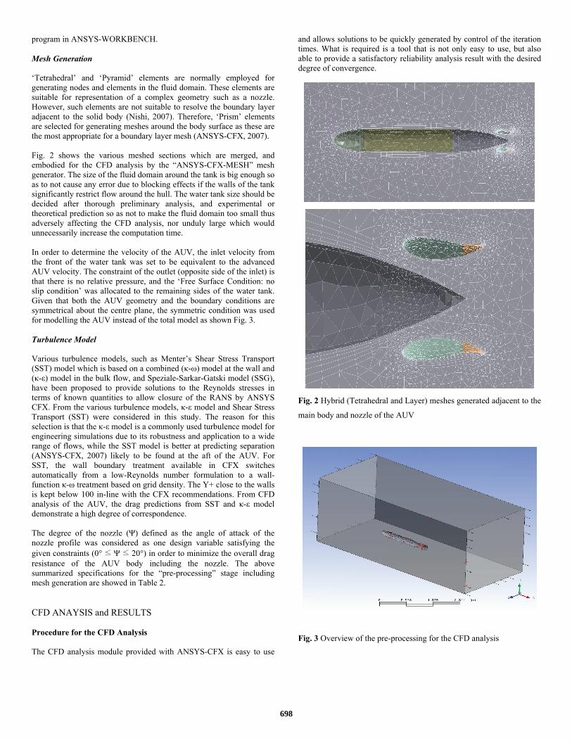
program in ANSYS-WORKBENCH. Mesh Generation ‘Tetrahedral’ and ‘Pyramid’ elements are normally employed for generating nodes and elements in the fluid domain. These elements are suitable for representation of a complex geometry such as a nozzle. However, such elements are not suitable to resolve the boundary layer adjacent to the solid body (Nishi, 2007). Therefore, ‘Prism’ elements are selected for generating meshes around the body surface as these are the most appropriate for a boundary layer mesh (ANSYS-CFX, 2007). Fig. 2 shows the various meshed sections which are merged, and embodied for the CFD analysis by the “ANSYS-CFX-MESH” mesh generator. The size of the fluid domain around the tank is big enough so as to not cause any error due to blocking effects if the walls of the tank significantly restrict flow around the hull. The water tank size should be decided after thorough preliminary analysis, and experimental or theoretical prediction so as not to make the fluid domain too small thus adversely affecting the CFD analysis, nor unduly large which would unnecessarily increase the computation time. In order to determine the velocity of the AUV, the inlet velocity from the front of the water tank was set to be equivalent to the advanced AUV velocity. The constraint of the outlet (opposite side of the inlet) is that there is no relative pressure, and the ‘Free Surface Condition: no slip condition’ was allocated to the remaining sides of the water tank. Given that both the AUV geometry and the boundary conditions are symmetrical about the centre plane, the symmetric condition was used for modelling the AUV instead of the total model as shown Fig. 3. Turbulence Model Various turbulence models, such as Menter’s Shear Stress Transport (SST) model which is based on a combined (κ-ω) model at the wall and (κ-ε) model in the bulk flow, and Speziale-Sarkar-Gatski model (SSG), have been proposed to provide solutions to the Reynolds stresses in terms of known quantities to allow closure of the RANS by ANSYS CFX. From the various turbulence models, κ-ε model and Shear Stress Transport (SST) were considered in this study. The reason for this selection is that the κ-ε model is a commonly used turbulence model for engineering simulations due to its robustness and application to a wide range of flows, while the SST model is better at predicting separation (ANSYS-CFX, 2007) likely to be found at the aft of the AUV. For SST, the wall boundary treatment available in CFX switches automatically from a low-Reynolds number formulation to a wall-function κ-ω treatment based on grid density. The Y+ close to the walls is kept below 100 in-line with the CFX recommendations. From CFD analysis of the AUV, the drag predictions from SST and κ-ε model demonstrate a high degree of correspondence. The degree of the nozzle (Ψ) defined as the angle of attack of the nozzle profile was considered as one design variable satisfying the given constraints (0° ≤ Ψ ≤ 20°) in order to minimize the overall drag resistance of the AUV body including the nozzle. The above summarized specifications for the “pre-processing” stage including mesh generation are showed in Table 2. CFD ANAYSIS and RESULTS Procedure for the CFD Analysis The CFD analysis module provided with ANSYS-CFX is easy to use

and allows solutions to be quickly generated by control of the iteration times. What is required is a tool that is not only easy to use, but also able to provide a satisfactory reliability analysis result with the desired degree of convergence.

Fig. 2 Hybrid (Tetrahedral and Layer) meshes generated adjacent to the

main body and nozzle of the AUV

Fig. 3 Overview of the pre-processing for the CFD analysis

698

Table 2. Principal conditions employed in the numerical computation

Water tank size 7,000×3,000×3,000 mm3

Turbulence model κ-ε model, Shear Stress

Transport (SST)

Reynolds number 8.73×105 ∼ 6.11×106

Radius, Length of the AUV 0.25 m, 2 m

Angle of attack of the nozzle 0° ∼ 20° (Design Variable)

Total no. of elements (nodes) 132,308 ∼ 158,611 (30,685 ∼ 45,303)

No. of Tetrahedral Max. 153,878

No. of Prisms; Pyramids Max. 1,313; Max. 3,420

If the results are satisfied at a certain value, a user can stop the run and move to “post-processing” to see the results. Fig. 4 shows the “solve-process” being monitored while ANSYS-CFX solver is running. Note that the value of the X-direction drag force of the AUV hull converged after nearly 30 iterations. The user, therefore, can decide the number of iteration for convergence and determine when to stop in order to save CPU time. Verification In order to ensure the verification of the CFD analysis, the bare hull of the AUV was employed, not considering nozzle part. The drag force predictions from the CFD results and the ‘ITTC 1957 correlation line’ have a high degree of correspondence as shown in Fig. 5. The results show that the form factor predicted by equation (2) is useful for the estimation. There are drag differences between ‘ANSYS-CFX’ and ‘ITTC 1957 correlation line’, because ANSYS-CFX considers the total drag while the ‘ITTC 1957 correlation line’ only considers the skin friction drag. The pressure and skin friction distribution along the AUV are shown in Fig. 6. The CFD results can thus be validated by the ‘ITTC 1957 correlation line’, and demonstrated to be reliable and useful for further research such as optimizing the nozzle shape. The CFD Results The empirical result, however, do not include the effects of separation of vortices at the stern. The detailed information about the velocity and pressure distribution of the AUV with nozzle can be extracted from the CFD code, ANSYS-CFX. The pressure distribution around the AUV (seen in Fig. 7 - 8) shows an even distribution except for the stagnation point at the bow of the hull. The maximum pressure (-1.822e-4Pa) occurs within part of nozzle, and is a negative pressure and higher compared to the pressure along the main body of the AUV. As the fluid passes through the nozzle its velocity increases as shown in Fig. 9. Along the parallel mid-body, the boundary layer grows and the flow is accelerated as it reaches the stern. Large vertical structures, which represent the wake region, form behind the stern as shown in Fig. 9. The flow is accelerated around the nozzle up to a maximum velocity of 2.167U0; the maximum velocity of the fluid in the nozzle is 6.5m/s, when the AUV velocity is 3m/s.

 (a) Default (Momentum etc.)

 (b) Defined by user (Drag)

Fig. 4 Monitoring during the CFD analysis process

699

Fig. 5 Comparisons of drag predictions for the AUV (w/o duct)

Fig. 6 Cp and Cf distribution around the AUV at 3 m/s (w/o duct)

Fig. 7 Pressure contour around the AUV hull at 3 m/s

 Fig. 8 Pressure distribution around the AUV at 3 m/s

Fig. 9 Velocity contour around the AUV hull at 3 m/s OPTIMIZATION BY THE CFD ANAYSIS Optimum Design Method A design optimization was carried out to find the optimum value of the nozzle angle, since it has a high sensitivity value with respect to the total resistance and drag, as well as AUV manoeuvrability. The object function for optimum design is the X-direction (+ is the advanced direction) drag force, and the constraint is the nozzle angle (0°～20°). For the purpose of finding the optimum value of the object function, the three tools, that is, 3D-CAD program, mesh generation program and ANSYS-DesignXplorer (DX), are linked together. ANSYS-DesignXplorer is the optimization program, which sets up the relations between input parameter from the 3D CAD program (DesignModeler (DM), AUTOCAD etc.) and output parameters. The typical application workflows of ANSYS-DesignXplorer comprise two different methods as shown in Fig. 10. The ANSYS-DesignXplorer provides three optimization methods; Design of Experiments (DOE), Variational

700

Technology (VT) and Design for Six Sigma (DFSS) (ANSYS-CFX, 2007). From the three methods, Design of Experiments (DOE) was employed for the optimization due to its simplicity and reliability. That is, DOE creates a matrix and builds an approximation model, and optimization is performed by sampling against this approximation method.

Fig. 10 The typical application workflow of ANSYS-DesigneXplorer The methods of ‘Design of Experiment (DOE)’ and ‘Direct Searching Method (What-if)’ were employed for the nozzle optimization as the optimum design methods. ‘Direct searching method’ is a crucial method but has a drawback, in that excessive computing effort is spent repeating the analysis process as many times as the number of samples. An alternative to ‘Direct Searching Method’ is the DOE method. Where possible the analysis for design variable(Ψ) in the constraints is carried out by the ‘Direct Searching Method’, whereas DOE is the method for carrying out a CFD analysis for an abstracted sample point only. In this way, it is, therefore, possible to reduce considerable CPU running time for the analysis. In this study, the sampling points are selected by Central Composite Design (CCD) to carry out the DOE method, before finding optimum value of the design variable. That is, sample points were abstracted by CCD, and the optimal design variable which has the optimum value of the object function was then identified. The DOE method by CCD sampling was verified by using the Direct Searching Method to ensure its reliability. Results of the Optimum Design The results of the CFD analysis conducted by DOE and Direct Searching Method are shown in Fig. 11 and Fig. 12, respectively. The results show that they have a similar trend and a high degree of correspondence. As shown in Fig. 11, the optimum value of the design variable (Ψ) was obtained as -11.11° from the CFD analysis by DOE, and the values of the object function (drag force) were 3.00 N (@ 1 m/s), 11.12 N(@ 2 m/s), and 23.98 N (@ 3 m/s). The result of the Direct Searching Method, which used for verifying the DOE-CCD result, showed that the optimum value of the design variable (Ψ) was obtained as -11°, and the values of object function were 2.98 N (@ 1 m/s), 11.05 N (@ 2 m/s), and 23.76 N (@ 3 m/s). The optimum value of the design variable

(Ψ) by DOE has a high correspondence with the Direct Searching Method, therefore, the results of the DOE method can be accepted to be reliable. From the results of the CFD analysis, shown in Fig. 13(a), it can be seen that if the nozzle angle is lower than the optimum angle (-11°), then the value of the object function (drag force) becomes much higher, even though mass flow of the water is a bit larger, when compared with the drag force at the optimum angle. On the other hand, if the nozzle angle is higher than optimum angle (-11°), not only does the value of the object function (drag force) become much higher, but also vortices can occur behind of the nozzle which reduce the nozzle efficiency, as shown in Fig. 13(c).

Fig. 11 X-directional drag force acting on the AUV (DOE)

Fig. 12 X-directional drag force acting on the AUV (Direct Searching

Method)

701

(a) 0° of the Nozzle (Initial value)

(b) -11° of the Nozzle (Optimum value)

(c) -20° of the Nozzle Fig. 13 Pressure and Velocity contour around the AUV at 3m/s

CONCLUSIONS In this paper, 3D modelling of an AUV shape, auto-meshing for element generation, and CFD analysis have been conducted using a commercial CFD program. As a result of the CFD analysis, pressure and velocity distribution around the AUV, and drag force were obtained. A CFD analysis was also carried out for finding the optimum value of a design value, i.e., the nozzle angle, based on given constraints. In summarizing the results of this study, we conclude the following, (1) In comparison with conventional methods, precise and reliable CFD results were obtained and verified by the ‘ITTC 1957 correlation line’. The results showed that the CFD method can be employed for estimation of the total resistance, even though the shape of the vehicle is complex. (2) Auto mesh generation with boundary layer inclusion can be used for faster convergence. The convergence time can be highly reduced by monitoring the object function and controlling the iteration times.

(3) Two possible optimum design methods, ‘Design of Experiment (DOE)’ and ‘Direct Searching Method (What-if)’, have been researched and employed for finding the optimum design value (nozzle angle) with the minimum value of the object function (drag force of the AUV). Future Work The velocity and pressure distribution around the AUV and drag estimation, which are difficult to obtain from an experimental tow tank test, were obtained by CFD analysis. Similarly, the optimum design value of the nozzle angle was also obtained using CFD analysis. The effect of the propulsion force have not however been considered in this paper. Relative rotation efficiency (ηR), thrust deduction fraction (t), and wake factor (w) of the nozzle should be carried out for more reliable optimization of the shape. A CFD analysis including a rotating propeller is now being studied, and will be verified by an experimental test in a tow tank. ACKNOWLEDGEMENTS The authors would like thank to Professor Yoshiki Nishi of Yokohama National University, Professor Wataru Koterayama, and Professor Masahiko Nakamura of Kyushu University in Japan for their practical, technical support, and productive international cooperation. REFERENCES ANSYS Inc. (2007). "ANSYS-CFX Ver. 11.0 Manual,” ANSYS Ltd,

2007 Hoerner, S.F. (1965). "Fluid-Dynamic Drag", Published by the Author Lim, SJ et al. (1971). "Principles of Naval Architecture - Korean

version", Dae-hwan text Co., pp 462-472. Michael, V. Jakuba (2003). “Modeling and Control of an Autonomous Underwater Vehicle with Combined Foil/Thruster Actuators,”

Massachusetts Institute of Technology, pp. 33-62. Nishi, Y., Kashiwagi, M., Koterayama, W., Nakamura, M., Samuel

S.Z.H., Yamamoto, I., Hyakudome, T. (2007). "Resistance and Propulsion Performance of an Underwater Vehicle Estimated by a CFD Method and Experiment," Proc 17th Annual Int Ocean and Polar Eng Conf, Lisbon, Portugal, ISOPE, Vol 2.

Phillips, A., Furlong, M., and Turnock, S.R. (2007). "The Use of Computational Fluid Dynamics to Access the Hull Resistance of Concept Autonomous Underwater Vehicles." OCEAN '07 IEEE Aberdeen.

Prestero, T. (2001). "Verification of a Six-Degree of Freedom Simulation Model for the REMUS Autonomous Underwater Vehicle", M. Sc. thesis at M. I. T., pp 14-19.

Seo, YK et al. (2005). "Computational Fluid Dynamics," Dong-A University, pp 187-201. Wilcox, D.C. (1998), “Turbulence Modeling for CFD”, DCW Industries.

702