a study on productive efficiency of sugarcane in
TRANSCRIPT

A STUDY ON PRODUCTIVE EFFICIENCY OF SUGARCANE
IN BANGLADESH: STATUS AND POTENTIALITY
Dissertation
Submitted in accordance with the requirements of the Bangladesh Agricultural University, Mymensingh
For the Degree of
DOCTOR OF PHILOSOPHY
BY
SAYEEDA KHATUN
Roll No. 4 Session 2003-04
Registration no. 12204 (1983-84)
Department of Agricultural Economics Bangladesh Agricultural University
Mymensingh
June 2011

A STUDY ON PRODUCTIVE EFFICIENCY OF SUGARCANE IN BANGLADESH: STATUS AND POTENTIALITY
Dissertation
Submitted in accordance with the requirements of the
Bangladesh Agricultural University, Mymensingh
for the Degree of
DOCTOR OF PHILOSOPHY
BY
SAYEEDA KHATUN
Roll No. 4 Session -2003-04
Registration no. 12204 (1983-84)
Approved as to style and contents by:
Professor Dr. Md. Habibur Rahman Supervisor
Professor Dr. M. Harun-Ar Rashid Co- Supervisor
Professor Tofazzal Hossain Miah Chairman,
Examination Committee Department of Agricultural Economics
June, 2011

Dedicated To My
Parents and Beloved Husband

Author’s Declaration
I declared that, except where otherwise stated, this dissertation is entirely my own work and has not been submitted in any form to any other university for any degree.
..........................
Sayeeda Khatun
Date:........................

ACKNOWLEDGEMENT At the inception, I wish to acknowledge the immeasurable grace and profound kindness of the “Almighty Allah” without whose desire I could not have materialized my dream to conclude this thesis. I would like to express my sincere gratitude to my respected teacher and supervisor Dr. Md. Habibur Rahman, Professor Department of Agricultural Economics, Bangladesh Agricultural University, Mymensingh, for his intense interest in this study and also his scholastic guidance, prompt comprehensive feedback, encouragement and patience throughout the entire duration of the research undertaken for this dissertation. I deem it a proud privilege to express my deep sense of gratitude and indebtedness for the kind cooperation of my co-supervisor Dr. M. Harun-Ar Rashid, Professor, Department of Agricultural Economics, Bangladesh Agricultural University, Mymensingh, whose insightful hints, stimulating suggestions and encouragement have helped me on numerous occasions throughout the study period. I would like to extend my sincere thankfulness to my respected and honorable teachers Professor Dr. M. A. Sattar Mandal, Professor, Department of Agricultural Economics and Vice- Chancellor, Bangladesh Agricultural University, Mymensingh, Professor Md. Tofazzal Hossain Miah, Professor Dr. W M H Jaim, Professor Dr. Rezaul Karim Talukder, Dr. Shamsul Alam, for their teaching and encouragement throughout my years as a student. My heartfelt thanks and gratitude are due to Dr.Taj Uddin, Professor and Head Department of Agricultural Economics, Professor Dr. Akteruzzaman, Associate Professor Md. Moniruzzaman, Assistant Professor Ismail Hossain Department of Agribusiness and Marketing, Bangladesh Agricultural University, Mymensingh whose support, cooperation, advice and inspiration were instrumental towards the completion of this work. I extend my grateful thanks and gratitude to the authority of Bangladesh Sugarcane Research Institute (BSRI) and Bangladesh Agricultural Research Council (BARC) for providing me scholarship to undertake this research I wish to thank Director General of Bangladesh Sugarcane Research Institute Dr. Gopal Chandra Paul, former Director Generals Dr. A. B. M. Mafizur Rahman and Dr. M.A. Mannan, Md. Nasir Uddin Khan, Ex-station in charge RSRS, Thakurgaon, Md. Mahmudul Alam, Head Agricultural Economics Division, Dr. Ibrahim Talukdar, Head, Pathology Division, Dr. Khalilur Rahman, Head, Agronomy and Farming Systems Research Division and my other colleagues at Bangladesh Sugarcane Research Institute for their immense interest, valuable advice and moral support to pursue my study. I also express my deepest gratitude to Julfikar Ali, Junior Officer, Rajshahi substation, Anwar Hossain, Junior Officer and Md. Tarajul Islam RSRS, Thakurgaon for their cooperation and inspiration for collecting data in my study period. My cordial thanks and appreciation are due to the farmers in the study area who supplied relevant information. I express my supreme gratitude to my parents, brothers, sisters and brother in laws for providing me affection, love, encouragement and support to make me capable educated and to get out in the world. In the day of my success, I would like to extend my gratitude and deep appreciation to all of them.

Last but not the least I extend my heartfelt thanks and appreciation to my beloved husband Dr. Md. Shamsur Rahman, Senior Scientific Officer, BSRI for his moral support, advice, sacrifice and inspiration to complete this thesis. The Author

69
BIOGRAPHICAL SKETCH
The author was born in 16th February, 1966 at Ghoshpara in Thakurgaon district of Bangladesh. She was the daughter of Md. Mansur Alam Mojibur Rahman and Mrs. Magfera Khatun and 3rd position among six brothers and sisters.
She completed her secondary school education from Thakurgaon Govt. Girls’ High School under Thakurgaon district and passed Secondary School Certificate (SSC) in 1981. She passed Higher Secondary Certificate (HSC) examination in 1983 from Thakurgaon Govt. College under Thakurgaon district. The author obtained both of her Bachelor of Science (Honors) in Agricultural Economics and Master of Science in Agricultural Economics degrees from Bangladesh Agricultural University (BAU), Mymensingh in 1987 and 1999 respectively.
The author started her professional career on 23rd December 1989as Scientific Officer (Agricultural Economics) at Farming System Research and Development Project, Bangladesh Sugarcane Research Institute (BSRI). After that, in 17th January, 1993 she joined as Scientific Officer (Agricultural Economics) in the main setup of Bangladesh Sugarcane Research Institute (BSRI). She was promoted as Senior Scientific Officer (SSO) on 5th August, 2007 and posted in Agricultural Economics Division, Bangladesh Sugarcane Research Institute, Ishurdi. Presently, she is working as Head of Agricultural Economics Division, BSRI. She has published 25 scientific articles in different national and international journals. She attended and successfully completed some in country professional training courses.
The author was awarded ARMP (Agricultural Research Management Project) scholarship for in country M.S. study in 1998 and successfully completed the degree. Moreover,she was also awarded a scholarship in 2004 funded by Bangladesh Agricultural Research Council (BARC) to pursue Ph. D. in Agricultural Economics at Bangladesh Agricultural University, Mymensingh. As part of Ph.D. study she carried out a piece of research work entitled “A study on productive efficiency of sugarcane in Bangladesh: Present status and potentiality”.
The author is happily married to Dr. Md. Shamsur Rahman, Senior Scientific Officer, Pathology Division, Bangladesh Sugarcane Research Institute.
Sayeeda Khatun
email: [email protected] Cell phone: 01716501655
70
A STUDY ON PRODUCTIVE EFFICIENCY OF SUGARCANE IN BANGLADESH: STATUS AND POTENTIALITY
S. Khatun
ABSTRACT Sugarcane is an important cash cum industrial crop in Bangladesh. It is the main raw material of
sugar and gur. Meeting the increasing demand for sugar and gur, a parallel sugar/gur production is required. This can be achieved by increasing the utilization of inputs and effectively organizing the management of production. The present study was undertaken in the selected areas viz., Rajshahi, Thakurgaon and Panchagar as well as Bangladesh to analyze the possibilities for improving productivity and reducing yield gap of sugarcane by increasing the farmers’ productive efficiency. The study employed farm level cross sectional data collected from 300 sample farmers during the period 2007/08. For growth rate and area response log linear and Nerlovian Partial Adjustment model were used. Time series data for the period 1975/76 to 2007/08 were also employed in this study. It was observed that the average yield was found to be 58.53 t/ha with the highest average at Rajshahi (62.30 t /ha) followed by Panchagar (57.80 t/ha) and Thakurgaon (55.80 t/ha). Among the farm categories, the large farmers produced the highest yield (59.83 t/ha) followed by medium (59.09 t/ha) and small (56.67 t/ha) farmers. The estimated stochastic frontier production function model showed that the human labour, animal labour, seed, urea, furadan 5 G 5 G and irrigation cost had a positive and significant impact on sugarcane production. The mean technical efficiency of sugarcane growers was 0.76 suggesting the existence of technical inefficiency by 24 percent. So, there was an ample scope to increase the farmers’ income and sugarcane yield by adopting the technologies by the farmers. Likewise, the mean allocative efficiency of 0.82 implied that there was an average level of 18 percent allocative inefficiency. The estimated cost frontier showed positively significant value of human labour and Muruate of Potash (MP) price positive and significant, which implied that increase of human labour and MP price resulted in the increase of sugarcane production cost. The average economic efficiency was found to be 0.62. Thus farmers’ economic efficiency could be enhanced by 38 percent through the improvement of both technical and allocative efficiency. The coefficients of sugarcane farming experience, plot visit by the field workers and training on sugarcane production were negatively significant in the inefficiency model implying that inefficiency decreases with the increases in farmers’ experience, visit by the field workers and training on sugarcane production. In the comparison of sugarcane and major crops the highest and positive growth rate of area and production were obtained by potato followed by wheat, lentil and rice. The growth rate of sugarcane area was positive but not significant although the production was stagnant. The growth rate of real price of all crops was negative but non significant, while that of sugarcane was negative and significant. This indicated that the sugarcane farmers received decreased real price. The instability of potato real price was the highest followed by that of lentil and wheat. Within the three sugar mills the sugarcane area instability of Thakurgaon was the highest followed by Rajshahi and Panchagar. For the country as a whole the lag one year area, price, relative price and relative price risk played a dominant role in determining current year allocation under sugarcane. The farmers did not take into consideration the relative yield risk and irrigated area for making a decision about the allocation of sugarcane area. Though irrigation had a positive impact on sugarcane production but the lag one year irrigated area had the negative impact on the current year sugarcane land allocation. When irrigated area increased the farmers were interested to allocate their land for cereals and other short growing high value crops. The yield gap-I was estimated at 23.28 t/ha which was the difference between experimental yield and potential farm yield and again the yield gap –II was 25.69 t/ha which was the difference between potential farm yield and actual farm level yield. The respondent reports a large number of technical and socio economic constraints which are the causes of yield gaps. The study suggests the existence of some gaps in sugarcane yield, which may be reduced through increasing efficiency. Government policy can be taken in order to increasing efficiency by farmers’ training, increased extension activities, subsidized input supply, price support and price declaration before planting season.
CONTENTS

71
Title Page
Declaration iv
Acknowledgement v
Biographical Sketch vii
Abstracts viii
Contents ix
List of Tables xiii
List of Figures xv
List of Appendix Tables xvii
Glossary xviii
Chapter 1 : INTRODUCTION 1-30
1.1 Agriculture in the Economy of Bangladesh 1
1.2 Sugarcane in Bangladesh 2
1. 3 Statement of the Study 7
1. 4 Objectives of the Study 10
1.5 Review of Literature of the Study 10
1.5.1 Productive Efficiency 10
1.5.2 Estimation of Growth Rate Related to Area, Production and Yields
18
1.5.3 Acreage Response/Supply Response 24
1.6 Organization of the Dissertation 29
Chapter 2 : METHODOLOGY
31-64
2.1 Theoretical and Conceptual Frameworks 31
2.1.1 Technical, Allocative and Economic Efficiency 32
2.1.2 Non-frontier Approaches 34
2.1.3 Frontier Approaches 35
2.1.3.1 Data Envelopment Analysis (DEA) 35
2.1.3.2 Stochastic Frontiers 36
2.1.4 Non- Parametric Frontier 37
2.1.5 Parametric Frontier 37
2.1.5.1 The Deterministic Frontier Approach 38
2.1.5.2 Stochastic Frontier
41
2.2 Sampling and Data Collection 46
2.2.1. Selection of The Samples and Sampling Techniques 46
72
2.2.2. Period of Data Collection 47
2.2.3. Data Collection Procedure and Collected Data 47
2.3 Measurement of Farmers’ Profitability 48
2.3.1. Analytical Technique of Profit Estimation 48
2.3.1.1. Estimation of Gross Returns 48
2.3.1.2. Estimation of Total Cost 49
2.3.1.3. Estimation of Profits 49
2.4 Determination of Productive Efficiency 50
2. 4.1 Analytical Techniques for Productive Efficiency 50
2.4.1 .1 Stochastic Frontier Production Function 50
2.4.1.2. Stochastic Frontier Cost Function 53
2.4.1.3 Technical Inefficiency Model 54
2.5 Growth Rates and Instability Analysis 55
2.5.1. Selection of the Study Area 56
2.5.2. Data Collection Procedure and Collected Data 56
2.5.3. Analytical Techniques of Growth Rate 56
2.6 Supply Response Analysis 58
2. 6.1. Analytical Techniques of Supply Response Analysis 59
2.7 Yield Gap Analysis 62
Chapter 3 : RESULTS AND DISCUSSION
3.1 COST, RETURN AND PROFITABILITY OF SUGARCANE PRODUCTION
63-79
3.1.1 Introduction 63 3.1.2 Variable Cost of Production 63 3.1.2.1 Human Labour Cost 63 3.1.2.2 Animal Labour Cost 66 3.1.2.3 Seed Cost 66 3.1.2.4 Organic Manure Cost 69 3.1.2.5 Fertilizer and Insecticide Cost 69 3.1.2.6 Irrigation Cost 70 3.1.2.7 Carrying Cost 70
3.1.3 Fixed Cost of Sugarcane Production 70
3.13.1. Land Use Cost 70
3.1.3.2 Interest on Operating Capital 71
3.1.4 Total Cost of Production 71
73
3.1.5 Yield and Gross Returns of Sugarcane Production 74
3.1.6 Net Returns of Sugarcane Production 75
3.1.7 Benefit Cost Ratio (BCR) 75
3.1.8 Summary of the Findings 78
3.2
EFFICIENCY AND DETERMINANTS OF EFFICIENCY IN SUGARCANE PRODUCTION
80-106
3.2.1 Introduction 80
3.2.2 Maximum Likelihood Estimates of Farm-specific Stochastic Frontier Production Function and Inefficiency Model
81
3.2.3 Maximum Likelihood Estimates of Location-specific Stochastic Frontier Production Function and Inefficiency Model
84
3.2.4 Maximum Likelihood Estimates of Farm-size Specific Stochastic Frontier Production Function and Inefficiency Model
87
3.2.5 Technical Efficiency and Its Distribution 91
3.2.6 Maximum Likelihood Estimates of Farm-specific Stochastic Frontier Cost Function and Economic Inefficiency Model
94
3.2.7 Maximum Likelihood Estimates of Location-specific Stochastic Frontier Cost Function and Economic Inefficiency Model
96
3.2.8 Maximum Likelihood Estimates of Farm-size Specific Stochastic Frontier Cost Function and Economic Inefficiency Model
99
3.2.9 Economic Efficiency and Its Distribution 101
3.2.1 Allocative Efficiency and Its Distribution 104 3.3
YIELD GAP AND CONSTRAINTS IN SUGARCANE PRODUCTION 107-117
3.3.1 Introduction 107
3.3.2 Yield Gap 107
3.3.3 Yield Gap due to Technical Inefficiency 111
3.3.4 Yield Constraints 111
3.3.5 3.3.4.1 Technical Constraints 112
3.3.4.2 Socio- Economic Constraints 113
3.3.5 Summary of the Findings 116
3.4 GROWTH AND INSTABILITY ANALYSIS OF AREA, PRODUCTION AND YIELD OF SUGARCANE
118-140
3.4.1 Introduction 118
3.4.2 Growth Rate Analysis 119
3.4.2.1 Compound Growth Rate in Area, Production, Yield and Price of Sugarcane and Other Major Agricultural Crops
127
3.4.2.2 Growth Rate in Sugarcane Area Among Different Locations 128
3.4.2.3 Growth Rate in Sugarcane Production Among Different 129
74
Locations
3.4.2.4 Growth Rate in Sugarcane Yield Among Different Locations
131
3.4.3 Instability of Sugarcane Area, Production Yields 132
3.4.3.1 Instability of Area, Production, Yield And Prices of Sugarcane And Other Crops
133
3.43.2 Instability of Sugarcane Area in Different Locations 134
3.4.3.3 Instability of Sugarcane Production in Different Locations 137
3.4.3.4 Instability of Sugarcane Yields in Different Locations 137
3.5.4 Summary of the Findings 138
3.5
SUPPLY RESPONSE ANALYSIS OF SUGARCANE PRODUCTION 141-147
3.5.1 Introduction 141
3.5.2 Supply Response Models of Sugarcane in Bangladesh 142
3.5.3 Short and Long –Run Elasticity and Coefficient of Adjustment 145
3.5.4 The test of Multicollinearity and Autocorrelation among the Explanatory Variables
147
3.55 Summary of the Findings 147
Chapter 4 : SUMMARY CONCLUSION AND POLICY IMPLICATION 139-148
4.1 Summary and Findings 139
4.2 Conclusions and Recommendation 145
4.3 Limitation of the Study 148
REFERENCES 149
List of Tables
Table Title Page
1.1 Agricultural sector and sub-sector share of GDP of Bangladesh at constant prices (Base: 1995-96).
2
1.2 Demand and supply of sugar and gur in Bangladesh 5
2.1 No. of sample in different locations and farm sizes 47
3.1.1 Per hectare production cost of sugarcane 64
3.1.2 Per hectare production cost of sugarcane at Rajshahi zone 65
3.1.3 Per hectare production cost of sugarcane at Thakurgaon zone 67

75
3.1.4 Per hectare production cost of sugarcane at Panchagar zone 68
3.1.5 Sugarcane production cost by different farm size groups (Tk./ha) 73
3.1.6 Per hectare cost, gross return and net return at different locations 73
3.1.7 Per hectare cost, gross return and net return at different locations 76
3.1.8 Per hectare cost, gross return and net return of different farm categories 76
3.2.1 Maximum likelihood estimates of the stochastic Cobb-Douglas frontier production and technical inefficiency model for sugarcane
82
3.2.2 Maximum likelihood estimates for parameters of location-specific Cobb-Douglas stochastic frontier production and technical inefficiency model for sugarcane
85
3.2.3 Maximum likelihood estimates for parameters of farm size-specific Cobb-Douglas stochastic frontier production and technical inefficiency model for sugarcane
89
3.2.4 Farm specific technical efficiency of sugarcane production 92
3.2.5 Frequency distribution of technical efficiency of sugarcane production 93
3.2.6 Maximum likelihood estimates for parameters of Cobb-Douglas stochastic normalized cost frontier and economic inefficiency model for sugarcane
95
3.2.7 Maximum likelihood estimates for parameters of l0cation-specific stochastic normalized cost frontier and economic inefficiency model for sugarcane
98
3.2.8 Maximum likelihood estimates for parameters of farm size-specific Cobb-Douglas stochastic normalized cost frontier and economic inefficiency effect model
100
3.2.9 Farm specific economic efficiency of sugarcane production 102
3.2.10 Frequency distribution of economic efficiency of sugarcane farmers 103
3.2.11 Farm specific allocative efficiency of sugarcane production 105
3.2.12 Frequency distribution of allocative efficiency of sugarcane farmers 106
3.3.1 Sugarcane yield realized and the estimated yield gap under different field situations
109
3.3.2 Estimated indices of yield gaps in sugarcane under different field situations 110
3.3.3 Yield gap of sugarcane due to technical inefficiency 111
3.3.4 Constraints and problems of sugarcane production as mentioned by the farmers 115
3.4.1 Compound growth rate of area, production, yield and price of major crops during the period of 1975/76 to 2007/08(in percent)
120
3.4.2 Compound growth rate of area, production and of sugarcane in three districts, sugar mill zone and overall Bangladesh for the period of 1975/76 to 2007/08.
123
3.4.3 Instabilities of area, production, yield and real prices of sugarcane and other crops
126
3.4.4 Instability index of area, production and yield in Bangladesh, mill zones and some selected districts during the period of 1975/76 to 2007/08.
127
3.4.5 Instability index of area, production and yield of sugarcane in Bangladesh in different period
128

76
3.4.6 Instability index of area, production and yield of sugarcane in Mill zone in different period
128
3.4.7 Instability index of area, production and yield of sugarcane in Panchagar in different period
128
3.4.8 Instability index of area, production and yield in Thakurgaon district in different period
130
3.4.9 Instability index of area, production and yield in Rajshahi district in different period.
130
3.5.1 Estimated parameters of Nerlovian Partial Adjustment Model of sugarcane in Bangladesh for the period from 1975/76 to 2007/08.
135
3.5.2 Estimated short-run and long-run elasticity 137
List of Figures
Figure Title Page
1.1 Different sugarcane production areas in Bangladesh 3
1.2 Utilization of sugarcane during 2007-08 4
2.1 Technical, allocative and economic efficiency 34
2.2 Technical efficiency of farms in relative input –output 40
2.3 Technical efficiency of stochastic frontier production. 45
3.1 Human labour cost for different locations for sugarcane cultivation 65
3.2 Human labour cost for different farm categories for sugarcane cultivation 65
3.3 Animal labour cost in different locations for sugarcane cultivation 67
3.4 Animal labour cost of different farm categories for sugarcane cultivation 67
3.5 Seed cost for different locations for sugarcane cultivation 68
3.6 Seed cost for different farm categories for sugarcane cultivation 68
3.7 Organic manure cost for different locations for sugarcane cultivation 72
3.8 Organic manure cost for different farm categories for sugarcane cultivation 72
3.9 Fertilizers and insecticides cost for sugarcane cultivation in different 72

77
locations
3.10 Fertilizers and insecticides cost for sugarcane cultivation for different farm categories
72
3.11 Irrigation cost for sugarcane cultivation in different locations 72
3.12 Irrigation cost for different farm categories for sugarcane cultivation 72
3.13 Percent shares of different input cost in production cost 74
3.14 Total production cost at different locations for sugarcane cultivation 74
3.15 Total production cost of different farm categories for sugarcane cultivation 74
3.16 Gross return, total cost and net returns at different locations 77
3.17 Gross return, total cost and net returns of different farm categories 77
3.18 Comparative benefit cost ratio of sugarcane cultivation at different locations 77
3.19 Comparative benefit cost ratio of sugarcane cultivation in different farm categories
78
3.20 Technical efficiency level of sugarcane producers in different locations 93
3.21 Technical efficiency level of sugarcane producers by different farm categories
93
3.22 Economic efficiency level of sugarcane producers in different locations 103
3.23 Economic efficiency level of sugarcane producers by different farm categories 103
3.24 Allocative efficiency level of sugarcane producers in different locations 106
3.25 Allocative efficiency level of sugarcane producers by different farm categories
106
3.26 Experimental station, potential farm and actual farm yield in sugarcane cultivation in Bangladesh
108
3.27 Growth rate of sugarcane area in different locations of Bangladesh 124
3.28 Growth rate of sugarcane production in different locations of Bangladesh 124
3.29 Growth rate of sugarcane yield in different locations of Bangladesh 124
3.30 Growth rate of sugarcane area, production and yield of sugarcane in Bangladesh
124

78
List of Appendix Tables
Table Title
Page
1 Area, production, yield and price of sugarcane in different years (1975/76 to 2007/08)
157
2 Sugar production, recovery and sugar price in different years (1975/76 to 2007/08)
158
3 Area, production and yield of sugarcane in Rajshahi Sugar mills in different years (1975/76 to 2007/08)
159
4 Area, production and yield of sugarcane in Thakurgaon Sugar mills in different years (1975/76 to 2007/08)
160
5 Area, production and yield of sugarcane in Panchagar Sugar mills in different years (1975/76 to 2007/08)
161
6 Area, production, yield and price of rice in different years (1975/76 to 2007/08)
162
7 Area, production, yield and price of wheat in different years (1975/76 to 2007/08)
163
8 Area, production, yield and price of potato in different years (1975/76 to 2007/08)
164
9 Area, production, yield and price of lentil in different years (1975/76 to 2007/08)
165
10 Per hectare cost and returns of sugarcane and sugarcane with intercrops 166
11 Cane yield, intercrop yield and adjusted cane yield under pared row system of planting
166
12 Zero order correlation matrix among the explanatory variables in Supply Response Model.
166
79
GLOSSARY
AE Allocative Efficiency
BARI Bangladesh Agricultural Research Institute
BBS Bangladesh Bureau of Statistics
BCR Benefit Cost Ratio
BSFIC Bangladesh Sugar and Food Industries Corporation
BSRI Bangladesh Sugarcane Research Institute
C-D Cobb-Douglas
CV Coefficient of Variation
DAE Department of Agricultural Extension
DAM Department of Agricultural Marketing
DEA Data Envelopment Analysis
EE Economic Efficiency
ha Hectare
HYV High Yielding Variety
I Instability Index
IRRI International Rice Research Institute
Kg Kilogram
Ln Natural Logarithm
LR Likelihood Ratio
MLE Maximum Likelihood Ratio
MP Muriate of Potash
OLS Ordinary Least Squares

80
R2 Coefficient of Determination
SD Standard Deviation
t Tonne
TE Technical Efficiency
Tk Taka (Bangladeshi Currency, 1 dollar = 70 Taka)
TSP Triple Super Phosphate
USDA United States Department of Agriculture
Chapter 1
INTRODUCTION
1.1 Agriculture in the Economy of Bangladesh
Bangladesh is a developing country in the world with high density of population
and unfavorable land-man ratio. Most of the people depend on agriculture. Agriculture being
a crucial sector of the economy, it is indispensable to develop this sector for attaining
economic growth and poverty alleviation. Since provision of food security, improving the
living standard and generation of employment opportunities of the huge population of the
country are directly linked to the development of agriculture, there has been continuous effort
by the government for the overall development of this sector. Agriculture plays a vital role in
the economy. It employs around 62 percent of the labour force of which 57 percent is in the
crop sector (Karim, 2005). This sector not only employs most of the national labour force but
also supplies food for human and animal consumption, raw materials for industrial
production and some value added commodities for export. In 2008-09, it contributed around
20.60 percent of the Gross Domestic Product (GDP). Among them, only crop sector
contributed around 11.55 percent (Table 1.1). The total cropped area is 12,141.70 thousand
hectares with 180 percent average cropping intensity (BBS, 2008).
Rice is the main food crop of Bangladesh which occupies 75 percent of total
cropped area and the remaining 25 percent is devoted to other crops which include wheat,
jute, sugarcane, oilseeds, pulses, vegetables, spices and condiments etc. In fact, the entire
growth in crop production can be explained by the growth in food grain production,

81
particularly rice. However, production of other crops such as sugarcane, vegetables, pulses,
oilseeds and fruits are rather disappointing. Currently, Bangladesh has been producing only
around 7.37 million tons of sugarcane (BSFIC, 2009), 0.28 million tons of pulses, 0.58
million tons of edible oilseeds (BBS, 2008) which are far less than the requirements of total
consumption in the country. It indicates unadjusted food plan which causes not only
imbalanced food supply but also malnutrition problem. In addition, the country is compelled
to import sugars, oils, pulses, etc. from abroad. Therefore, crop diversification is essential in
order to achieve the goal of overall nutritional self-sufficiency, balanced food supply,
production of industrial raw materials and so on. Furthermore, it is also needed to encourage
the production of cash crop. .
Table 1.1 Agricultural sector and sub-sector share of GDP of Bangladesh at constant prices (Base: 1995-96).
Sector/sub-sector 2004-05 2005-06 2006-07 2007-08 2008-09 1. Agriculture 17.27 16.98 16.64 16.23 16.03
a. Crops 12.51 12.28 12.00 11.70 11.55
b. Livestock 2.95 2.92 2.88 2.79 2.73
c. Forestry 1.82 1.79 1.76 1.75 1.75
2. Fisheries 5.00 4.86 4.73 4.64 4.57
Total 22.97 21.84 21.37 20.87 20.60
Sources: BBS, 2008, 2009
1. 2 Sugarcane in Bangladesh
In Bangladesh, sugarcane is the second most important cash crop after jute. It is not
only the most important cash crop but also an important food cum industrial crop and the
main raw material for sugar and gur industries of Bangladesh. Although it ranks second
among cash crops but fourth among the major field crops in the country which covers about
2.05 percent of the cultivable land. More than 0.60 million farm families are dependent on
sugar industries for their subsistence. At present, 15 sugar mills are in operation under
Bangladesh Sugar and Food Industries Corporation (BSFIC). Most of the sugar mills of
Bangladesh are located in the North Western zones of the country where concentration of
sugarcane cultivation is higher. Sugarcane cultivation is mainly concentrated in the low-
rainfall belts of the North Western parts in Bangladesh. Less productive river basins (char

82
lands) are also being increasingly brought under sugarcane cultivation. It is also traditionally
grown in the high lands of the central parts of Bangladesh. Currently, on an average,
sugarcane is grown in 0.18 million hectare of land of which almost 50% is located in the mill
zones, where sugarcane is mostly utilized for sugar production and remaining 50% is situated
in the non-mill zone, which is used for gur and juice production (Alam, et.al,2005).

83
In 2007-08, Bangladesh produced 7.37 million tones of sugarcane. Out of that 2.29
million tons (31%) were used by sugar mills to produce 0.16 to 0.20 million tons of sugar;
4.03 million tons (55%) were used to produce 0.30 million tons of gur and remaining 1.05
million tons (14%) were used for seed and chewing purposes (Figure 1.2). Per capita
consumption of sugar and gur in Bangladesh is less than 10 kg per annum. But in India,
China, Thailand, , Brazil, Pakistan and EU it is 19, 10, 36, , 54, 23 and 34 kg respectively
(World Sugar, 2009). According to Food and Agricultural Organization (FAO) per head
annual necessity of sugar is 13 kg (Ali and Ali, 1990) and as such present requirement of
sugar and gur for 143 million people, the annual demand is 1.87 million tons. However, our
current (2007-08) domestic sugar and gur production was 0.16 and 0.41 million tons
respectively and imported sugar was 1.20 million tons. Total supply of sugar and gur
was1.78 million tons and the deficit was 0.09 million tons (Table 1.2). To meet that demand,
the country’s annual sugar and gur production should be increased, otherwise, people must
consume less amounts of sugar and gur than their requirements. Therefore, there is an ample
scope of increasing sugarcane production for sugar and gur which can not only meet the
national demand but also increase the contribution to Gross Domestic product (GDP)
including savings of foreign currency. Economic development of any country greatly depends
on the availability of exportable commodity and foreign exchange. Bangladesh spends a large
amount of foreign currency for sugar importation every year which impacts negatively on the
national economy.
Figure 1.1 Different sugarcane producing areas in Bangladesh
2.29 MMT (31%)
1.03 MMT (14%)
4.03 MMT (55%)
Sugar production Gur production Seed & Chewing

84
Figure 1.2: Utilization of sugarcane during 2007-08
Table 1.2 Demand and supply of sugar and gur in Bangladesh
Crushing Season
Populat-ion
(million)
Demand of sugar & gur ('000 tonne)
(per capita 13 kg)
Sugar production
('000 tonne)
Sugar import
('000 tonne)
Gur Production
('000 tonne)
Total supply of sugar & gur ('000
tonne)
Shortages ('000 tonne)
1998-99 129.08 1678.00 152.98 151.00 378.83 682.81 995.19
1999-00 131.49 1709.00 123.50 115.00 432.45 670.95 1038.05
2000-01 132.00 1716.00 98.35 328.00 604.24 1030.59 685.41
2001-02 133.00 1729.00 204.33 105.00 453.67 763 966
2002-03 134.00 1742.00 177.40 600.00 508.08 1285.48 456.52
2003-04 135.20 1757.60 119.15 440.00 395.57 954.72 802.88
2004-05 137.00 1781.00 106.65 687.00 409.19 1202.84 578.16
2005-06 138.80 1804.40 133.28 625.00 307.04 1065.32 739.08
2006-07 140.60 1827.80 165.00 594.00 281.39 1040.39 787.41
2007-08 143.91 1870.83 163.84 1200.00 415.33 1779.17 91.66
Source : BBS 1998-2008
Sugarcane plays a significant role in the economy of Bangladesh. Sugar industry is
providing employment nearly of 16000 persons including development works. It plays an
important role to develop infrastructure in rural areas, rural employment, income of the farm
families, contribution to national exchequer, foreign exchange saving and value addition to
the sugar, gur and by-product industries (Alam et al. 2005). Sugar falls under carbohydrate
group of foods which is an important constituent of human diet. It is an indispensable item
for proper activities of brain. For each person, 77 mg glucose (simple form of sugar) is
required every minute for perfect function of brain. Sugarcane is the main source of white
sugar and gur. Sugar may provide 10-13% of the calories. It is used for manufacturing fruits
and vegetable preservatives, sweets, fruit drops, confectionery, toffees, biscuits, sugar cubes,
etc. The main by-products of sugar industries are molasses, bagasse, and pressmud. The
molasses can be utilized for producing spirit and alcohol. At present, Brazil and many other

85
countries use bio-ethanol from sugarcane as an alternative of fossil fuel and it is being used in
transport engine. Sugarcane is the world’s largest source of fermented ethanol. It is one of the
most photosynthetic efficient plants - about 2.5 % photosynthetic efficiency on an annual
basis under optimum agricultural conditions. From sugarcane bagasses, high quality paper
may be produced. Pressmud is also an excellent source of organic matter. A further advantage
is that bagasse can be used as a convenient on-site electricity source. The green leaves, cane
tops and young suckers are used as high quality cattle feed. After harvesting sugarcane, the
dry leaves and crop residues can be used as fuel. Considering the above aspects, there is a
great impact of sugarcane in Bangladesh in respect of food, energy, employment, soil health
improvement and in development of overall national economy. Sugarcane is cultivated in
almost all the districts of Bangladesh. It concentrates mainly the greater districts of Rajshahi,
Kustia, Jessore, Rangpur, Dinajpur, Bogra, Pabna, Faridpur, Barisal, Dhaka and
Mymensingh. At present sugarcane occupies an important place in cropping pattern of
Bangladesh and brings large dividends to growers, but its yield and production has become
stagnant for the last so many years due to our limited resources and other unavoidable factors.
The national average yield of sugarcane in Bangladesh is 46 tonne per hectare which is less
than that of other countries of the world. Average cane yields in Pakistan, India, Thailand,
China and Brazil were 53.20 t/ha, 66.93 t/ha, 63.71 t/ha, 80.82 t/ha and 74.42 t/ha
respectively (FAO 2007).
The Government of Bangladesh is emphasizing the attainment of self-sufficiency in
sugar and gur production by stabilizing sugarcane area and increasing the yield. Bangladesh
Sugarcane Research Institute (BSRI) has recommended a number of improved production
technologies from planting to harvesting with a view to increase the per hectare yield of
sugarcane through varietals improvement, better management of water resources, providing
fertilizers and other inputs properly and improved cropping patterns. So, Sugar Mills,
Department of Agricultural Extension (DAE), Non government Organizations (NGOs) and
other agencies have also been working for a long time to increase the production of sugarcane
per unit area by adopting those practices.
1.3 Statement of the Study

86
Sugarcane is one of the agro-based industrial crops of Bangladesh and sustains the
economy of large number of rural people. It is the main source of sugar and gur. About 70%
of total world’s sugar is produced from sugarcane and 30% from sugar beet (Jamil and
Gopang, 2004). Except diabetic patients, more than 99 percent of the people take sugar/gur
and sugar products everyday. It makes the food palatable and contributes on brain
development of human being. So it is an essential food item with great importance. The
present production of sugarcane can meet neither the total sugar nor nutrient requirements of
the country. Considering these circumstances, the government of Bangladesh is determined to
increase sugar and gur production by increasing the area of sugarcane and thereby sugarcane
has been included in the national food security programme.
The producers are profit-maximizers who take decisions based on expected
profitability. Generally, while making production decisions, the farmers consider returns
against expected cost. Sometimes it is mentioned that the yield they receive does not cover
the cost of production. In this connection, this study on sugarcane production is imperative in
order to determine its prosperity under different categories of farmers. This study is expected
to quantify the farmers’ profitability and existing potential of resources at farm level.
Currently, the sugar sector of Bangladesh is experiencing a great crisis. The sugar production
is very low compared to our national requirements. The emerged shortfall of sugar is partially
met from importation and smuggling. Every year, 0.2-0.3 million tons of sugar is being
imported and near about 0.1 million tons comes through black marketing (Miah et al. 2003).
To overcome the crisis, boosting up the production of sugarcane is essential. By increasing
area it is not possible, since total cultivable area is decreasing day by day due to the increased
use of land for non-agricultural purposes. Therefore, it is needed to increase productivity
through improving efficiency. Estimation on the extent of efficiency can also help to decide
whether to improve efficiency or to develop new technologies to raise sugarcane
productivity. If one knows the existing efficiency level of farmers in using the inputs for
sugarcane production then viable plans could be taken to increase sugarcane production. If
the farmers are found to be technically inefficient, production can be increased to a large
extent with the existing level of inputs and available technology by rearranging input
combinations. On the other hand, if the farmers are found to be technically efficient, then the

87
government can increase investment on information and education and can try to promote
new technologies in order to increase production. Efficiency measurement is the first step in a
process that might lead to substantial resource savings. These resource savings have
important implications for both policy formulation and firm management.
Although a good number of studies have been conducted on efficiency and growth of
major foodgrains but they did not deal with performance of specific sugarcane. However, no
study on production efficiency in sugarcane farming has been undertaken so far. In fact, hard
data efficiency of sugarcane is scanty. The present study is, therefore, a pioneering attempt to
examine the productive efficiency of sugarcane production of the farmers of Bangladesh.
Yield variation is one of the major problems of sugarcane production in Bangladesh.
The concept of yield gaps comes from the country study carried out by the International Rice
Research Institute in the 1970s which make a quantitative difference between the potential
yield and actual yield (Gomez et al. 1979). The estimates of sugarcane yield obtained in
research field, on-farm demonstration and farmers’ field for different eco-systems will be the
yield gap.
Although, sugarcane is a profitable crop with ensured market but increased yield,
production and area of sugarcane are not adequate in our country to meet our requirement.
Sugarcane area in 1973-74 was 1,47,368 hectares, which increased by 1,66,802 hectares
during 1983-84 and by 1,65,992 hectares during 2002-03. Yield of sugarcane was at a
standstill around 42 t/ha in 1973-74, 41 t/ha in 1983-84 and 46 t/ha in 2007-08 which is
significantly lower than that of other countries. The slow increasing trend in area, production
and productivity of sugarcane in recent years has become a serious concern of the planners
and policy makers in the country. In order to explore the present status and potentialities of
sugarcane, it is, therefore essential to examine the past performance of sugarcane. Analysis of
growth rates and fluctuation of area, production, yield and price of sugarcane is useful for
policy making since they help to understand the magnitude and direction of the changes that
are taking place.
The cultivation of sugarcane in Bangladesh is not free from production constraints,
which are mostly technical and socioeconomic in nature. Lack of technological knowledge

88
packages include use of high yield and high sugar content varieties, clean seed utilization,
proper dose of fertilizers and pesticides applications, proper irrigation and drainage facilities
etc. On the other hand, socioeconomic constraints include particularly poor financial
facilities, poor marketing facilities, lack of purzi (supply order of cane to the mills), etc. The
aims of the present study are to analyze the above issues in order to recommend a suitable
suggestion.
The present study may be useful both at micro and macro levels. Results and
information gathered in this study will be useful to farmers, researchers, extension workers,
non-government organizations (NGOs) and policy makers in choosing or suggesting better
production technology to have higher yield and to maximize profit of farmers within their
resource endowment.
1.4 Objectives of the Study:
1. to estimate the profitability of sugarcane production.
2. to measure the technical, economic and allocative efficiency of sugarcane
production.
3. to find out the yield gap between potential and actual yield of sugarcane.
4. to estimate the growth rate and instability of sugarcane and its competitive crops in
terms of area, production and yield.
5. to determine the area response of sugarcane production.
6. to suggest some policy guidelines about sugarcane crop.
1.5 Review of Literature
A number of studies of different crops have been done at home and abroad and
investigated the technical, allocative and economic efficiency, growth and instability and the
area response. But in case of sugarcane such study has not yet been done. This section is
concentrated with the review of literature related to productive efficiency, growth rate related
to area, production and yields and supply response studies.

89
1.5.1 Productive efficiency
Farrell (1957) introduced the analysis of efficiency in the economic literature. There
has been a wide-ranging collection of papers and articles devoted to the measurement of
productive efficiency. A close link has always been found between measurement of
efficiency and the use of frontier function. Different techniques have been utilized to either
calculate or estimate these frontier functions.
Kaliranjan (1981) illustrated the advantage of using a stochastic production frontier
model for the analysis of yield variability in paddy production. The approach not only allows
for randomness in the estimates as in conventional methods, but also explicity allows for the
inter-farmer variability in using the technology. it is argued that this is a more appropriate
methodology when examining issues of productivity differences than conventional
production function models as estimated in most econometric studies. this methodology
allows farmers to be technically inefficient relative to their frontier rather than to some
sample norm estimated by a conventional production function. The result of the empirical
study demonstrated the workability and potential usefulness of the methodology and showed
that in this case: individual farmer variability (technical inefficiency) was the major cause for
yield variability but not the random variability.
Kalirajan and Flinn (1983) studied technical efficiency of rice farms in the Philippines
using the stochastic frontier production. Their findings indicated that the technical efficiency
of rice farmers varied widely averaging around 50%. Farmers’ experience and contact with
extension agents significantly and positively contributed to higher technical efficiency, while
method of planting had a negative effect on technical efficiency.
Ali and Flinn (1989) estimated both firm-specific technical and firm and input
specific allocative efficiency of farmers for rice production in Pakistan using stochastic
frontier profit function. Their estimates indicated an average technical inefficiency of 23%
and an allocative technical inefficiency of 5%. While farmer’s education had the highest and
most significant contribution to both technical and allocative efficiency, late planting, late

90
fertilizer application, and irrigation problems significantly affected negative technical and
allocative efficiency.
Ali et al. (1990) studied the agricultural production efficiency in four cropping region
on the Punjab province of Pakistan and compared the relative efficiency on the basis of
probabilistic frontier production function estimated from whole farm survey data for the year
1984-85. They found that gross income of farmers might be increased by 13% at the current
levels of resource use if the production gap between ‘best practice’ and average farmers
become narrowed down in all cropping regions. This would increase profit up to 40%.
Ureta and Rieger (1991) examined dairy farm efficiency using stochastic frontier and
neoclassical duality model. The stochastic model was used to analyze technical, economic
and allocative efficiency for a sample of New England dairy farms. Cross sectional data for a
sample of 511 New England dairy farms (excluding the sate of Rhode Island) were used to
estimate a Cobb-Douglas stochastic production frontier which is the basis for deriving a
scholastic cost frontier and related efficiency measures. The data used in the study were from
Dairy Herd Improvement (DHI) production records for the calendar year 1984 combined with
data obtained from a mail survey. The analysis showed that, for the sample of dairy farms,
average technical efficiency was 83 percent, average economic efficiency was 70.2 percent,
and average allocative efficiency was 84.6 percent. The results suggested that mean economic
efficiency for the farmers in the sample was about 70 percent and that, on average, there was
little difference between technical (83.0 percent) and allocative (84.6 percent) efficiency.
Analysis of the relationship between efficiency and four socioeconomic variables-farm size,
education, extension, and experience revealed that despite some statistically significant
associations, efficiency levels were not markedly affected by these variables.
Battese et al. (1996) investigated technical inefficiencies of production of wheat
farmers in four districts of Pakistan. A single stage model for estimating technical
inefficiencies of production in a stochastic frontier production function was applied in the
analysis of panel data. Results showed that the mean technical efficiencies for wheat farmers
in Faisalabad. Attock, Badin and Dir were 0.79, 0.58, 0.57 and 0.77 respectively. The
individual technical efficiencies in Faisalabad tended to increase over the years involved.
Relative to the frontiers in each district, the highest levels of technical efficiencies were in
Faisalabad with Dir being a close second. On average, these farmers were close to 80 percent
of the maximum technical efficiency. The technical inefficiency effects associated with the

91
production of wheat in Faisalabad were significantly related to the age and schooling of
farmers.
Tadesse and Krishnamoorthy (1997) measured the level of technical efficiency across
ecological zones and farm size groups in paddy farms of the Southern Indian state of
Tamil Nadu. The study revealed that 90% of the variation in output among Paddy (IR-20)
farms in the state is due to differences in technical efficiency. Land, animal power and
fertilizers have significant influence on the level of Paddy production. Varying from 0.59
to 0.97 the mean technical efficiency was found to be 0.83. There was a scope for
increasing paddy production by 17% through adopting the technology and the techniques
used by the best practices of paddy farms. A significant variation was observed in the
mean level of technical efficiency among the four major rice growing zones of the state
and farmers operating on small and medium sized farms achieved a higher level of
technical efficiency than those with large holdings. The farm size- ecological zone
interaction effects also reveal that small and medium sized paddy farms in zone-II and III,
respectively, are operating at a higher level of technical efficiency than all other farms.
Seyoum et al. (1998) investigated the technical efficiency of two samples of maize
producer in two districts in Eastern Ethiopia who were either within or outside the
Sasakawa Global 2000 project and the other involving farmers outside this programme.
They used stochastic frontier production function in which technical inefficiency effects
are assumed to be functions of the age and education of the farmers and extension
contact. The results indicated that farmers within the project are more technically more
efficient than farmers outside the project, relative to their respective technologies The
result also indicated that the small scale farmers within the project had significantly
higher outputs and productivity and the technically infficiency effects in maize
production and negatively related to the hours of extension advice, indicated that the
programme involved should be expanded on a larger scale.
Ahmad and Shami (1999) estimated the sericulture production structure and measured
the farm-level technical efficiency in Pakistan. The result revealed that most of the farmers
involved in this enterprise were illiterate. This industry is further characterized by
inappropriate rearing sheds, complete lack of extension service, and dependence on

92
government forests for mulberry leaves facing peak season shortage, supply of poor quality
silkworm seed and improper processing and marketing facilities. Labour shares more than 70
percent of the total cost of production and however, promises reasonably high return on
investment. Stochastic production frontier analysis indicated that the sericulture enterprise
faces increasing returns to scale. Average technical efficiency was found to be 0.88 with a
minimum of 0.37 and a maximum of 0.98, leaving significant scope for improvement in
productivity and thus profitability. The result further showed that technical efficiency was
positively associated with the size of the activity associated
Sharma et al. (1999) carried out a study to measure comparative efficiency of the two
frontier approaches. Firm-specific factors affecting productive efficiencies were also
analyzed, Finally swine producers’ potential for reducing cost through improved efficiency is
also examined, variables returns to scale (VRS), the mean technical, allocative and economic
efficiency indices were 75.9%, 75.8% and 57.1% respectively, for the parametric approach
and 75.9%, 80.3% and 60.3% for DEA (Data envelopment analysis): while for the constant
returns to scale (CRS) they were74.5%, 73.9% and 54.7% respectively, for the parametric
approach and 64.3%, 71.4% and 75.7% for DEA. Thus the results from both approaches
reveal considerable inefficiencies in swine production in Hawii. The estimated mean
technical and economic efficiencies obtained from the parametric technique were higher than
those from DEA for CRS models but quite similar for VRS models, which allocative
efficiencies were generally higher in DEA. Based on this result by operating at the efficient
frontier the sample swine produces would be able to reduce their production costs by 38-46%
depending upon the method and returns to scale.
Mythili and Shanmugan (2000) conducted a study to estimate the technical
inefficiency of individual farmers using an unbalanced panel data of 234 rice farmers in
Tamil Nadu for the period 1990-91 to 1992-93. The maximum likelihood method was used to
estimate the frontier function. The result reveals that the technical efficiency varies widely
(ranging from 46.5 percent to 96.7 percent) across sample farms and was time invariant. The
mean technical efficiency was computed as 82 percent, which indicated that on an average,
the realized output can be increased by 18 percent without only additional resources. The

93
existing gap between released and potential yield highlights the need for improving farmers’
practice through extension services and training programmes.
Rahman et al. (2000) estimated farm-specific technical efficiency of rice in
Bangladesh using a translog stochastic production frontier. Variables considered in the
technical inefficiency effect model including age, education and experience of farmers,
extension contact and farm size. The study reveled that the output per farm can be increased
on average by 12% for Boro, 9% for Aus and 19% for Aman through the efficient use of
existing production technology without incurring any additional production costs. The study
also revealed that technical efficiency increased with the increase in age, experience, and
extension contact and farm size. Farmers with larger farms were technically more efficient
than farmers with smaller operations.
Backshoodeh and Thomson (2001) conducted a study on input and output technical
efficiencies of wheat production in Kerman, Iran in 1995. They developed a simple relation
between farm level output-based technical efficiency measure (the Timmer index) and input
based measures (the Koop index). In this study, Timmer and Kopp indexes of technical
efficiency were estimated for 164 farms using Cobb-Douglas frontier production function
with a composite error term. The results show that the mean values of the Timmer and Kopp
technical efficiency indices were over 0.90 but the one-quarter of the farms were below 0.90
for the Timmer index and below 0.87 for Kopp index. The level of efficiency was found to be
related to farm size, small and large farms were shown to be more technically efficient than
medium sized farms, and efficiency was found to be affected by some input ratios such as the
ratio of fertilizer to seed. With the given inputs, the production of wheat could be increased
by 7.2% on average through making all farms 100% efficient. Alternatively, inputs could be
reduced by 9% on average to produce the same amount of wheat output. However the study
finally revealed that, since wheat produces may be able to adapt their production process
more easily and quickly by implementing new techniques, i.e. by more efficient combination
of inputs, than by adopting new technology, correction of input over-use can be regarded as a
policy with speedy of limited effect in this case.
Chaudhry (2001) analyzed the technical efficiency of Pakistani farmers by farm level
input-output data for 1997-98 with reference to fertilizer used. For this purpose he used

94
Cobb-Douglas frontier production function. The study revealed that education of farm
operator and irrigation source has a more pronounced effect on technical efficiency. The
tenant operated farms were more efficient than those operated by owners or owner-cum-
tenants. Total fertilizer nutrients applied as well as the balanced mix of nutrients affect
technical efficiency positively. The study also reveled that the contact of farmers with
extension agents and/or agricultural scientists had a positive effect on efficiency. Application
of farmyard manure also affected technical efficiency positively. The results imply that the
investment in human capital in rural areas should be encouraged.
Kabir and Alam (2001) estimated technical and allocative efficiency of irrigated
sugarcane farms in Northwest and Southwest regions in Bangladesh in 1997-98. The study
examined the possibility of raising sugarcane productivity by improving technical and
allocative efficiency of farms in sugarcane production. He used Cobb-Douglas production
function to estimate the efficiency. The study revealed that the mean technical and allocative
efficiency of irrigated sugarcane were 0.61 and 0.60 respectively. The study concluded that
there is enough scope of increasing sugarcane output using the available inputs and
technology.
The study by Kamruzzaman et al. (2001) attempted to examine the effect of credit on
yield gap and technical efficiency of Boro paddy production in a selected area of Comilla
district. The results indicated that credit receivers achieved higher (82.12%) amount of
potential yield than the credit non-receivers (78.99% of the on farm trial conducted by
BRRI). It showed that the yield gap was higher for the credit non–receivers than for the credit
receivers. So it was observed that credit has positive impact on reducing yield gap. The study
also identified that mechanical power cost, irrigation cost, application of urea, application of
MP and credit dummy had positive impact on reducing yield gap while human labour, and
TSP application and age had negative impact on reducing yield gap. So, farmers have to
increase the use of mechanical power, irrigation water, urea, MP and credit money while they
need to decrease the use of human labour and TSP for reducing yield gap. Credits also
shower positive impact on increasing technical efficiency. Technical efficiency was higher
for credit receivers than the non-receivers according to tenure status, age category, and
educational status, frequency of extension conducted.

95
Ahmed et al. (2002) analyzed productivity, efficiency and sustainability of wheat in
Pakistan. They used farm level survey data to estimate the stochastic frontier production
incorporating efficiency effect. The study reveals that the agricultural farmers has a
significant positive effect on farm efficiency implying that as age increases, the farm
efficiency declines. The reason for this relationship may be due to the fact the aged farmers
may be unwilling to take risk. The farmers’ education emerges as an important factor in
enhancing agricultural productivity. Educated farmers usually have better access to
information about prices and state of technology and its use. The farm to market distance
variable has a significant and positive association with inefficiency. To reduce farm
inefficiencies the farmers have provide with easy excess on favorable terms to credit. The
study also reveals that tenants are statistically more efficient than owner and owner-cum
tenants. The large farmers are relatively more technically efficient than the small farmers.
Wheat productivity is significantly higher on farms having access to more reliable irrigation
system – i.e. cannel and tube well both, as compared to the non irrigated farms and farm
relying only on a single relatively less ensured source of irrigation, i.e. either cannel or tube
well.
Rao et al. (2003) attempted to examine the levels of technical efficiency in the
production and attempted to identify the factors associated with technical efficiency of three
major crops, viz., rice, groundnut and cotton, in the state of Andhra Pradesh in India. For this
purpose stochastic frontier production model was used. The study revealed that average
technical efficiency of rice, groundnut and cotton were 85, 79, 72 percent respectively. It was
suggested that there was considerable scope to increase yields of the crops in the existing
conditions of input use and technology. The study also revealed that technical efficiency
levels were negatively significant for age, education and percent area under the crop. The
negative coefficients suggest that as the age, education and percent area under the crop
improved/ increases the inefficiency decreases. So, efforts should be strengthened to promote
both formal and informal education.
Shanmugam (2003) analysed the economics of cultivation of major crops- rice,
groundnut and cotton in Tamil Nadu by estimating the stochastic frontier production function
and farm-specific technical efficiencies using farm level collected data for the period 1990-91

96
to 1992-93. The result indicates that land and labour inputs are the significant determinants of
output for all crops in the state. Fertilizer variable influences positively on the yield levels of
rice and cotton crops. The other cost variable is significant only in irrigated groundnut. The
returns to scale parameters for production of almost all crops are close to one (constant
returns to scale). There are considerable evidences that the observed outputs of all principal
crops selected for the study are less than their respective potential outputs due to technical
inefficiency. The average technical efficiency values of raising rice I, rice II, irrigated
groundnut, rainfed groundnut and cotton in Tamil Nadu are 82, 82, 68, 76 and 68 percent
respectively. The study also reveals that the technical efficiency of raising irrigated
groundnut is relatively high in own land cultivation as compared to that in leased land
cultivation. The result also indicates that providing middle and higher education of farm
families would increase the agricultural productivity. The small farmers can better follow the
practices followed by the large farmers to reap more yield or they can shift from cotton
cultivation to some other crops for which they are efficient.
Baksh (2003) studied economic efficiency and sustainability of wheat production in
Bangladesh by applying stochastic frontier production function of a Cobb-Douglas type
functional form. He observed that farm specific technical efficiency varied among farmer to
farmer and ranged from 0.62 to 0.96 with a mean of 0.88 in Dinajpur district followed by
efficiency that ranged from 0.51 to 0.96 with a mean of 0.96 in Rangpur district. The frontier
farmers received higher yield by following optimum seeding time, using more urea, TSP,
gypsum, manure and applying more frequently irrigation water with modest use of seed rate
and human labour at both the sites.
Islam (2003) studied profitability and technical efficiency of wheat production in
some selected areas of Bangladesh. He applied stochastic frontier production with Cobb-
Dauglas functional form and found mean technical efficiency level of 70 percent. The
medium farmers were technically more efficient than small and large farmers. He found that
coefficient of farming experience and frequency of extension contact to be negative and
significant implying that the farmers with farming experience and more extension contact
were technically less efficient.

97
Reddy and Sen (2004) attempted to find the existence of technical inefficiency in the
production of rice in the Sone canal command area of the state of Bihar. The study revealed
that yield of rice can be considerably improved by reducing inefficiency, without increasing
the level of inputs. It also revealed that technical inefficiency in the production of rice is
negatively related with farm size, education of the farmer, experience, extension contacts and
percentage of good land and positively related with age and fragmentation of the land. Caste
of the farmer and location of the farm in the canal command do not have any influence on
inefficiency. Similarly the number of farm workers in the family did not show any pattern
with inefficiency. To reduce inefficiency in the production of rice and wheat measures like
encouraging co-operative type of farming, land consolidation, improving literacy rate,
strengthening extension services and providing alternate employment opportunities should be
taken up in that area.
1.5.2 Estimation of Growth Rate Related to Area, Production and Yields
The growth rate analysis in crop output has occupied an important place in
agricultural economics literature, particularly in India. The increase in agricultural production
has traditionally been explained in terms of the area and yield components. However, Minhas
and Vaidyanathan (1965) added third components, the cropping pattern. They demonstrated
an ‘additive scheme of decomposition’ to measure the relative contributions of area, yield and
cropping pattern components and an interaction components of cropping pattern and yield to
the growth in agricultural output in India. The pioneering work of Minhas and Vaidyanathan
(1965) attracted many researchers (Venkataramanan and Prahladachar, 1980; Sondi and
Singh, 1975; Misra, 1971) to study the relative contributions of different sources to the
growth in agricultural output at the state or all India level.
Alagh and Sharma (1980) estimated the growth rates for food grains, sugarcane major
oilseeds, cotton, jute and mesta for the country as a whole and major States for the following
three times periods : (i) Period I – 1960-61 to 1969-70; (ii) Period II – 1969-70 to 1978 -79
and (iii) Period III – 1960-61 to 1978-79. It is interesting to note that as compared to the
position in period I in which the regional spread of agricultural growth was somewhat
limited, i.e., predominated by Punjab and Haryana, in period II the growth pattern is more

98
evenly spread across regions. The study reveled that, during the period I, the trend growth
rate of food grains output was 1.85 percent and rose to 2.74 percent in period II and taking
longer time span of period III (1960-61 to 1978-79), the per annum trend growth rate was
2.77 percent. Growth rate of output was 2.29, 3.42 and 2.93 percent per annum for sugarcane,
0.28, 1.35 and 1.57 percent for major oilseeds, 1.62, 0.31 and 3.38 percent for cotton and
-2.18, 1.61 and 0.16 percent per annum during the period of I, II and III respectively in all
over the India. It is concluded that the estimated agricultural growth rate for the period II is
higher than the period I.
Hossain (1984) analyzed the long-term (1949-84) growth of Bangladesh agriculture
and factors contributing to it. He calculated the long term trend rate of growth to be 2.5
percent per annum for cereals, 1.1 percent for cash crops and 1.5 percent for non cereal crops.
During the period under study pulse showed negative growth rate of -0.51 per cent whereas
oilseeds and potato recorded a rate of 1.82 and 8.17 per cent respectively. However, during
the period 1970-71 to 1983-84 the growth rates of pulses, oilseeds and potato were -0.56,
1.12 and 3.53 percent only. On estimation of relative contribution of relative contribution of
different elements it was found that during 1970-1983 increase in crop yield contributed 69.2
percent to the growth in crop output, whereas acreage expansion contributed only 14.3
percent.
Kaushik (1993) analyzed the pattern of growth and instability of crop output in India
in general and oilseeds in particular. He used secondary data for the period of 1968-69 to
1991-92. The data were collected from government of India (1990, 1993). Compound growth
rate by an exponential growth models btaYt += was used to estimate the growth rate of
production, acreage and productivity. It was found that no significant difference existed
between the growth rates in wheat and total food grains. Whereas, the difference was
statistically significant in the case of rice and total oil seed.
Instability is one of the important decision parameters in development dynamics and
more so in the context of agricultural production. It is found that the increasing tendency of
yield instability in the case of oilseeds can be attributed to the fact that oilseeds are grown
mostly in the not irrigated areas and are dependent on rain. But area brought under irrigation
was delivered to the production of food grains to the neglected of oilseed crops. Hence,
99
oilseeds production mostly under rainfed condition becomes a risky enterprise under poor
management resulting in unstable yields. The study further reveals that the fluctuation in
yield is the major cause for the fluctuation in the output and hence the fluctuations in yields
have to be controlled to bring in stability in the output.
Tripaty and Gowda (1993) studied the growth, instability and area response of
groundnut in Orissa. They used secondary data of Agricultural Statistics, published by the
Directorate of Agriculture and Food Production, Government of Orissa for the post-green
revolution period (1970/71 to 1990/91). For estimating compound growth rate they used the
growth model ubln t aln lnY ++= . Nerlovian lagged adjustment model was used to
examine the area response of groundnut. The study revealed that the area was the dominant
source of growth of output during the post-green revolution period. Groundnut production
increases significantly at the rate of 10.29% per year which was primarily due to a significant
expansion of area (10.36%). Per hectare yield of groundnut was almost stagnant in the state.
Price incentive had played an important role for phenomenal increase in area of this crop. The
improvements per hectare yield of groundnut in some districts was attributable to favorable
climate conditions, increase in area under irrigation and dissemination of new crop
production technologies to farmers’ fields through ‘Training and Visit’ extension net work.
This study further revealed that in a majority of the districts instability in yield was lower
than instability than production. It indicated that irrigation favorably influenced the area
under groundnut in the static during the post revolution period.
Dhakal (1993) examined the performance of crops in Bangladesh by utilizing the time
series data from 1977 to 1999. The findings showed that except the tuber crops, all other crop
recorded significant positive growth in area and production and that all the crops recorded
significant positive growth in prices. In case of all the pulses, price was the main component
of growth in the value of output although in case of mungbean area and cropping pattern
changes were more influential. Yield contributed the most to the growth of lentil but the least
to the mungbean. In cases of oilseeds and tuber crops too price was the main component of
growth, although area and crop-mix effects were also equally responsible in some oilseed
crops. In case of tuber crops price was the only component responsible for the grown in the
value of output for sweet potato and a major component for potato. The acreage response
functions of the crops revealed that in most cases only the coefficient attached to the lagged

100
acreage turned out to be significant while the relative profitability with HYV boro had little
influence in the acreage allocation decision to different minor crops.
Alam (1996) estimated yield, price and income instability of different crops in Jessore
district during the period 1973-74 to 1989-90. An index of instability was computed for
examining the degree of instability in crop production. In case of product prices, the
coefficient of variation ranged from a minimum of about 9 percent for wheat (MV) to a
maximum of 56 percent for garlic. The study revealed also that the price instability of all the
food crops (rice and wheat) was less compared to other crops, indicating the significance of
the institutional intervention in marketing of food crops. It was also observed that price
instability was higher than yield instability of wheat. They mentioned that considering the CV
of prices and gross returns, cereal crops were found to be less risky compared to the other
crops (non-cereals). The study concluded that agriculture in Jessore district was highly
unstable and risky, characterized by fluctuations in farm income resulting from instability in
both yield and price.
Dhindsa et al. (1997) analyzed the growth behavior of pulses and examined the
acreage response of various factors determining the decisions regarding allocation of land
among different pulse crops in Punjab and its various sub-regions. The study was based on
secondary data covering the period of 1966-67 to 1991-92. Compound growth rate was used
for estimating growth performance by the least squares method of fitting the exponential
function and area response relationships had been estimated with the help of the Nerlovian
adjustment model. The study revealed that the performance of pulses in the state of Punjab
had been found to be dismal during the post-green revolution period. The negative growth of
production of pulses can be mainly attributed to a decline in area and stagnancy in the yield
of various pulses crops. The supply response analysis of pulse crops revealed that the non-
price variables rather than price variables were significant in determining the area response of
various pulses crops (except moog) in the state and its various sub regions. The study also
revealed that an increase in gross irrigated area in Punjab would cause a reduction in the area
under various pulse crops (except moog). This is due to the fact that old varieties of most of
these crops give lower yield on irrigated land whereas new varieties of wheat and rice give
very high yield on irrigated land.

101
Yadev and Singh (1997) analyzed in their study that the changes in the area,
production and productivity of rice and wheat in Bihar during the period from 1970-72 to
1994-95. The study was based on secondary data. A decade wise analysis of area, production
and productivity of rice and wheat crops in the state clearly indicated that the break through
in agriculture was really biased towards wheat. In Bihar during the post green revolution
period from 1970-71 to 1994-95, wheat acreage increased by 57 percent. However, a major
expansion in wheat acreage was observed during 1970-71 to 1975-76 by nearly 127 percent.
During the period from 1970-71 to 1974-75 production and productivity of wheat also
witnessed a major increase by 244 and 120 percent respectively. During the post-green
revolution period from 1970-71 to 1974-75, rice cultivation did not experience any change in
its area, production and productivity in Bihar.
Singh et al. (1998) analysed growth and instability of area, production and productivity of
principal crops i.e. food grain, rice, wheat, maize and pulse in North Bihar. The
production of almost all the principal crops increased during green revolution period;
however, the increase was more pronounced in wheat and maize crops. The study
revealed that their production recorded positive growth rates during post green revolution
period. Wheat recorded positive growth rates in area, across the zone over different sub-
periods. There had not been substantial increase in area under rice during the period. The
study also revealed that instability indicated that wheat, maize and arhar witnessed a
continuous decline in instability over the period. The declining instability in the
production of these crops had been caused mainly by adoption of improved technology in
crop production. The spectacular growth in production was associated with increase in
instability but it started declining after the perfection in technology.
Barua and Alam (2000) attempted to assess the growth, fluctuation and price
flexibility of Aus, Aman, Boro, Wheat and Jute crops during the last two decades of the
twentieth century (1980-81 to 1998-99). Real prices of all they have been falling significantly
during the study period, the price instability was higher than area and yield instability for all
these crops studied. The extent of real price fluctuation was higher relative to area,
production and yield of all the crops. It was observed that supply of Aus, Wheat and Jute
production played insignificant role to determine their own post-harvest prices, but Boro,

102
Aman and Aus production had significant role on the prices of crops of Aus, Wheat and Jute
through cross effects. On the other hand, Aman and Boro production had significant
influence on post-harvest price determination of these rice varieties as revealed by flexibility
co- efficient.
Singh and Srivastava (2003) examined the growth and instability in sugarcane
production in Uttar Pradesh. The study made use of time series data on area, production and
productivity of sugarcane for Western, Eastern and Central regions to the period 1980-81 to
1998-99 based on secondary data sources. Semi log equations were fitted to estimate
compound growth and instability was measured through co-efficient of variation analysis
using detrained data. The study reveals that acreage, production and yield growth rate of
sugarcane are 1.60, 3.48 and 1.85 percent per annum respectively in Uttar Pradesh. Sugarcane
production variability is the maximum in the central region, followed by in the eastern region.
Finally, the study also reveals that the instability is the major source of production instability.
It is possible that most of the fluctuation are due to pricing and cane payment policies.
1.5.3 Acreage response/supply response
Estimating of supply response would require the setting up of an economic model.
The basic hypothesis would be that the area under a crop responds to stimuli like price,
rainfall or yield change. The supply estimates depended on the specifications of variables
followed. Some of the major findings of these studies are summarized below.
The seminal study by Nerlove (1958) on the dynamic supply response of agricultural
product served as an important methodological step. Nerlove developed a way to quantify the
unobservable expected ‘Normal’ price in terms of past-realized prices with the help of
expectation model and explained the corresponding variations in area response with the help
of adjustment model. Out of these two models, Nerlov’s 2nd model ‘the adjustment lag’ is
well-known. This model presents a more realistic picture by incorporating distributed lags
and thereby introducing a realistic assumption about the farmers’ adjustment behavior. In this
model of area response non static expectation is either implicitly or explicitly taken care of.
The preference to this model is also due to its computational and interpretational ease over
expectations model. It facilities the estimation of the long run and better estimates of supply

103
elasticities. Basically, the Nerlovian model attempts to reduce the very complex process of
area response to various economic and non-economic changes into a pair of adjustment
equations which are purely of a statistical nature. Further, it is assumed that over a period of
analysis, the adjustment coefficients are static in nature, irrespective of any structural changes
in the economy. The merit of the model depends on how best it is able to explain a real world
situation. And Nerlove has succeeded to a very great extent, in explaining the behavior of
farmers in the United States of America, with the help of model.
Nerlove’s concept and approach thus gave a new horizon to supply studies. Following
the pioneering work of Nerlove, a large number of studies were undertaken using the
framework. The original model has since been modified in various ways to suit the needs of
the analysis. Among the studies, the work of Krishna (1963), Rao and Krishna (1965), Kaul
(1967), Behrman (1968), Alam (1992), etc. were the pioneering work for the developing
countries following the Nerlove model. From the above studies, it was observed that
modification to the model have tended to concentrate on the inclusion of extra explanatory
variables of particular interest in the situation under investigation and change in the concepts
of variables used by Nerlove. However, underlying dynamic form of the model remained
unchanged.
Krishna (1963) studied the supply response of eleven farm commodities of the
undivided Punjab, based on time series data for 1913-14 to 1945-46. Estimates of supply
elasticities were obtained with Nerlovian adjustment lag model. He formulated the model as
follows:
tt1t1t1t*t uhWgZcYbPAX ++++++= −−−
)XB(XXX 1t*t1tt −− −=−
The reduced form of equation being,
t1t6t51t41t31t20t vXbWbZbYbPbaX ++++++= −−−−
Where,
a0=aB, b2=bB, b3=cB, b4=gB, b5=hB, b6=(1-B) and vt=But

104
*tX is the standard irrigated area that farmer would plant in the year t
Jha (1970) estimated the impact of relative price and some non-price variables on
sugarcane acreage and measured the changes in the nature and magnitude of relationship
between variables over time. For this purpose district wise data on acreage, price and other
variables for the period of 1912-13 to1964-65 were collected from secondary sources. In
order to examine changes over time, separate analyses were conducted for the 1912-13 to
1964-65, 1933-34 to 1964-65 and 1950-51 to 1964-65 segments of the time-series. Additional
regression were also run for three independent segments - 1912-13 to1932-33, 1933-34 to
1949-50 and 1950-51 to 1964-65 for a more precise picture of those changes. The Nerlovian
adjustment lag model was used to obtain the response the relation. The study reveled that the
relative price variable appears consistently significant. For identical time periods the relative
sugarcane price equations provide a better measure of the relationship than do the relative gur
ones. The coefficients for the price variable are generally higher and more significant in the
1950-51 to 1964-65 than in other equations. If higher relative gur price was expected, farmers
plant more acreage under sugarcane. The study also reveled that lagged yield did not show
any significant influence in any time period equation with relative gur prices. Except for the
1912-13 to 1964-65 equation, rainfall was found to be significant in others, indicating that
favorable moisture conditions during planting time encourage a little more area to be put
under the crop. Acreage under wheat (competing crops of sugarcane) was found to be
significant only in the 1912-13 to 1964-65 equation. The study further reveled that there
being no deliberate attempt to allocate areas under sugarcane, it was planted only after the
grains quota was full filled.
Sabur (1983) in his research work elaborated on the growth rates in area,
production and productivity, behavior of price, area response to price and price variation,
elasticity of demand and concluded with a projected demand and supply position of potato.
Nerlovian adjustment lagged model was used, using time series data of area, price, rainfall
etc. for the period of 1960-61 to 1981-82.
The last year’s area played a pivotal role in determining area under potato in
determining area under potato. The short-run and long-run elasticity differed significantly due
to low value of coefficient of adjustment .On the other hand, in case of all the districts, except

105
Dhaka, the short and long run elasticities differed slightly due to high value of coefficient of
adjustment. But in these entire situation the short-run elasticities as obtained from traditional
model was higher than those for Nerlovian model. The results indicated that the farmers in
the northern districts were more responsive to the change in economic environment. The
result did not support the superiority of Nerlovian adjustment lag model over the traditional
one in explaining the supply price relationship. In his study, the dynamic model equations
were estimated through the Ordinary least square (OLS) method and serial correlation was
tested with Durbin-Watson‘d’ statistics.
Sangawan (1985) attempted to analyze the cropping pattern changes in terms of
varying responses of individual crops to price and non price factors. To measure the
magnitudes and nature of various supply shifters, the acreage supply equations have been
estimated with Nerlove’s partial adjustment adaptive expectation model. The study revealed
that the cash crops, e.g., rapeseed/mustard seed, American cotton, sugarcane and ground nut
were more responsive than food crops. Among the food crops the elasticity of barely was
higher than that of wheat, etc. Nowadays, barley is being substituted by wheat in
consumption but due to its demand from the beer industry, farmers may produce it for
market. Acreage under wheat, barley, sugarcane, groundnut and cotton positively responded
to yield changes while bajra acreage responded negatively to yield. Acreage under wheat,
barley, sugarcane, groundnut, and cotton were positively related to both price and yield
changes. And mostly (except sugarcane) these were the crops which significantly gained in
their areas. Water availability, i.e., sowing-season rainfall, shows significant positive impact
on areas under gram, rapeseed/mustered seed, barely, and rice. Rahman (1986) estimated the
supply response of some crops in Bangladesh for the period 1972-73 to 1981-82 by
employing ordinary least squares techniques. He estimated supply functions for both acreage
and output for most of the crops, using partial adjustment model. Instead of annual average
retail or wholesale prices, Rahman used deflated harvest prices; the deflator being the
wholesale price index. The price elasticity of cash crops, e.g., jute, tobacco, cotton and
sugarcane were relatively higher as one would expect. The price elasticity of boro rice which
was not produced mainly for subsistence was also high. It was evident that aman and aus rice
could not be influenced significantly by output price policies. However, the boro rice crop be
substantially influenced by a price support policy. The rapid expansion in production of

106
wheat took place in response to the demand for food grain and under substantial government
support. The supply price elasticity was statistically significant for all cash crops except
cotton. The magnitude of the short run price elasticity of jute, tobacco, sugarcane, rape and
mustard, till and groundnuts were 0.51, 0.39, 0.64, 0.80 and 0.30 and the long run elasticity
for lentil was 0.75.
Khan and Iqbal (1991) first estimated dynamic supply response of ten major crops
(Wheat, rice, cotton, sugarcane, maize, pearl millet, sorghum, barley, chickpea and oilseeds)
in Pakistan using time series data for the period 1956/57- 1986/87. Supply response was
estimated under three alternative expectation schemes, namely, Perfect Foresight, Static
Expectations and Adaptive Expectations to investigate the sensitivity of supply parameters
under different expectation schemes. The Dynamic supply response model under static
expectations performed the best. It was found that farmers in Pakistan did respond to changes
in relative prices as well as yields in their crop allocation decisions. The results suggested that
price policy alone would not be sufficient to raise agricultural production in Pakistan. Area
elasticity with respect to yield exceeded area elasticity with respect to prices for many crops,
therefore, an input subsidy policy as well as price policy should be pursued in order to
increase production.
Alam (1992) studied the supply response of major crops for the period 1971-72 to
1987-88 using Nerlovian dynamic models through an Instrumental Variable Nonlinear Least
Squares (IV-NLS) Maximum Likelihood (IV-ML) method. He took into consideration the
relative product price changes and other influencing factors like rainfall, yield trends, price
and yield risks for estimating the supply responses of all rice varieties and jute. He observed
that the jute yield increase was not influenced by the preceding seasonal prices but was
conditioned by the availability of improved seed varieties and extension services. Jute areas
were highly responsive to sowing period rainfall and jute, aus price ratio. Farmers were risk
averse to jute price fluctuations. He also observed that rice areas were highly responsive to
deflated product price. Responsiveness was higher for the modern varieties where weather
risks had been lower. Farmers were also averse to price risks. He showed that availability of
adequate rainfall during sowing planting periods of the non irrigated rice crops was the most
constraining limiting factor in area allocation.

107
Jaforullah (1992) examined the responses of sugarcane growers to price and yield
risks and identify the factors responsible for variations in sugarcane area in the mill zones of
Bangladesh during the period of 1947-81. For this purpose secondary data from different
sources of sugarcane area, yield and price, jute yield and prices were collected. He used
adaptive expectations model, partial adjustment model and partial adjustment-extrapolative
expectations model. The study revealed that the partial adjustment model had come out as the
best model of all considered. The results revealed that both short and long run price
elasticities of sugarcane area were less than one, implying inelastic area response to
sugarcane price. However, the long-run elasticities were greater than the short-run elasticities.
This is because sugarcane growers have more time in adjusting their area under the crop in
the long run than in the short run. The elasticity of sugarcane area with respect to yield was
higher than its elasticity with respect to price. In deciding on sugarcane area allocation,
farmers respond positively to changes in sugarcane price and negatively to changes in jute
price. The results also revealed that the sugarcane yield relative to jute yield per hectare, the
sugarcane price risk relative to jute price risk, and the relative sugarcane yield risk to jute
yield risk in making decisions with respect to allocation of area between these two crops.
This result suggested that the government should undertake measures to increase sugarcane
yield per hectare to complement appropriate pricing policy.
Singh and Lal (1993) studied to examine the impact of both price and non-price
factors on supply (acreage} of edible oilseeds in the major growing states in the country. For
this study three oilseeds namely, groundnut, rape seed and mustard and their major growing
states were selected for analysis. For the selected states time-series data pertaining to the
period 1968-69 to 1990-91 on area, yield, rainfall, net irrigated area, farm harvested price of
edible oilseeds and their two major competing crops in the respective states were used for the
study. In this study three oilseeds, namely, groundnut, rape seed and mustard and their major
growing states were selected for analysis. For the selected states time-series data pertaining
to the period 1968-69 to 1990-91 on area, yield, rainfall, net irrigated, farm harvest price of
edible oilseeds and their two major competing crops in the respective states were used for the
study. For each state the Nerlovian adjustment lag supply response model, excluding and
including risk variables, were estimated considering one competing crop at a time. The
results of the study revealed that supply-price relationship of oilseeds was positive but week
in most of the states. In certain cases the oilseeds acreage response to relative price was

108
significant. The yield of own crop had positive impact on acreage of crops in almost all the
states. In several cases, the elasticity coefficient of this variable was statistically significant.
On the other hand, the yield of competing crops had a detrained impact on acreage of oilseeds
in most of the states. The other non-price factors such as expansion of net irrigated area in the
state and rainfall in the seasons showed a week positive and negative impact on acreage of
oilseeds in almost all the states. The farmer’s supply response to risk caused by price as well
as yield of oilseeds and their competing crops was weak in most of the cases. This indicates
that the oilseeds are not much concerned about price and risks.
Yunus (1993) estimated the supply responses equation for a number of crops using
time-series data for the period 1972-73 to 1988-89. The gross cropped area of food grain, rice
and other crops were used for estimating the acreage response functions. However, individual
crops such as boro rice and wheat were price responsive. The short run and long run price
elasticity for boro and wheat were 0.50, 0.61 and 2.86, 5.24 respectively. The study reveals
that boro and wheat cultivated to meet farmers’ subsistence needs. The acreage responses of
some crops such as pulses, oilseeds and spices were very week. Almost all of the cash crops
viz. jute, tobacco, cotton and sugarcane were relatively high responsive to price change as
one would expect. For some crops, the acreage response to yield change was found to be
strong and statistically significant. In almost all other cases the yield elasticity estimates were
several times higher than price elasticity estimates. This suggests that farmers responded
much more strongly to yield augmenting (declining) technology than to price changes. Yield
augmenting technology operates allocation of land between subsistence crops and cash crops
would no longer be a zero sum game. There is thus no real conflict between food self-
sufficiency and cash crop production.
Chaudhary (2000) represented an attempt at estimating the farmer supply response to
price and non-price factors with respect to the allocation of the cultivated area among crops
of wheat, cotton, rice, sugarcane and maize. To estimate farmers’ supply response he used
Nerlove’s partial adjustment and adaptive expectation model. The study reveled that the high
values of R 2 and F indicates good fit and the overall significance of the supply response
functions. The significant effect of the lagged dependent variable had been found to highly
significant affect the acreage allocation among crops. The expected prices had been more
pronounced in acreage allocation for cotton and sugarcane than for wheat and rice. The effect

109
of the expected prices on acreage allocation among crops also depended on whether was food
or cash crops. Area allocation to food crops was in general expected to show less variations
compared to that of cash crops. Irrigated area had positively affected the area planted to both
wheat and cotton.
The present research was designed to study, among others, the profitability,
productive efficiency, supply response, yield gap, etc. of sugarcane production in
Bangladesh. In order to find a suitable model for frontier analysis prominent studies were
reviewed. Particularly in the context of Bangladesh Rahman et al. (2000), Kabir and Alam
(2001), Kamruzzaman et al. (2001), Baksh (2003) and Islam (2003) were prominent studies.
Most of the studies were concerned with crops other than sugarcane. The only study
conducted by Kabir and Alam (2001) was concerned with sugarcane but it did not study the
productive efficiency of sugarcane. Thus, the present research seeks to explore the productive
efficiency of sugarcane in Bangladesh taking intellectual inputs from related studies. To
make the research comprehensive, supply response, yield gap, production and yield growth
etc., were also be included. No, study on sugarcane was accomplished by incorporating yield
gap, supply response and frontier production functions in Bangladesh. The present research is
designed to fulfill that task. Thus the findings from this research will be useful to research
institutes, researchers and policy makers. Researchers will get inputs from this research for
carrying out further research on this line.
1.6 Organization of the Dissertation
Keeping the above objectives in view, the present dissertation is organized in 4
chapters. Chapter 1 presents Bangladesh agriculture and its economy, sugarcane in the
economy of Bangladesh, Statement of the problems and objectives of the study. A brief
review of the previous studies related to yield, productive efficiency, growth rate and supply
response analysis are presented in Chapter 1 also. Chapter 2 discusses the basic concepts of
technical, allocative and economic efficiency, stochastic frontier function, advantages and
limitations of different estimation techniques and methods and measurement. Methodology
used for the selection of study area and sample farms, collection of data and techniques used
for empirical estimation of efficiency are also presented in Chapter 2. Chapter 3 describes the

110
costs, returns and profitability of sugarcane cultivation, efficiency and determinants of
efficiency in sugarcane production, growth rate and its instability in sugarcane production,
supply response and yield gap. Constraints in sugarcane production were also discussed in
Chapter 3. Finally, conclusion, recommendation and policy implication are highlighted in the
Chapter 4.
Chapter 2
METHODOLOGY

111
The main purpose of the study is to investigate into a number of areas for which
theoretical frameworks, methodology and analytical techniques differ considerably. It aims to
assess the economic profitability, measure productive efficiency, estimate the growth and
instability, estimate supply response, yield gap and constraints to yield gap in sugarcane
production. For better understanding of the methodology to be used in each of the aspects, in
this chapter sequential step of work would be followed to discuss elaborately for instance,
theoretical framework, selection of the study areas, selection of the samples, preparation of
the survey schedule, selection of the study period, data collection, and analytical technique.
2.1 Theoretical and Conceptual Frameworks
The measurement of productive efficiency of a farm comparative to other farms or to
a standard practice has been of interest to agricultural economists for the last five decades.
The problem of measuring productive efficiency is important to both economist and
academicians and policy makers. Producers have to take decision on the basis of availability
of scarce resources in their command. Producers must decide what to produce, how much to
produce, what method of production to use, where to sell and buy. All these decisions of
producers are due to scarcity or limited resources. The measurement of the productive
efficiency of a farm relative to other farmers or to the “best practices” in an industry has long
been of interest to agricultural economists. From a theoretical point of view, there has been a
spirited exchange about the relative importance of various components of firm efficiency
(Leibenstein, 1966, 1977, Comanor and Leibenstein 1969; Stigler 1976). From an applied
perspective, measuring efficiency is important because this is the first step in a process that
might lead to substantial resource savings. These resource savings have important
implications for both policy formulation and firm management (Bravo-Ureta and Rieger
1991).This chapter is devoted to the theoretical and conceptual frameworks of efficiency
measurement where, technical, allocative and economic efficiency, their measurement
approaches and estimation procedure are discussed.
2.1.1 Technical, Allocative and Economic Efficiency
The theory of production is mainly concerned with maximizing profit or in some
instances minimizing cost. Both are indicative of economic efficiency. Productive efficiency
has three parts-technical efficiency, allocative efficiency, and economic efficiency. Farrell

112
(1957) disaggregated economic efficiency into price or allocative efficiency and technical
efficiency. Technical efficiency (TE) of a farm can be defined as the ability and willingness
of the farm to obtain the maximum possible output with a specified endowment of inputs
(represented by a frontier production function), given the technology and environmental
conditions surrounding the farm (Mythili and Shanmugam, 2000). A technically efficient
farm will operate on its frontier production function. Thus it is an indicator of productivity of
the farm and the variation in TE can reflect the productivity differences among farms. It helps
hunting the potentiality of the existing level of technology used by the producers. In other
words, a farm is considered to be technically efficient if it operates on an isoquant rather than
interior to isoquant. Technical inefficiency refers to failure to operate on the production
frontier. Technical efficiency (TE), on the other hand is related to the fixed resources, which
are part of the environment and exogenous of the firm (Yotopoulos and Nugent, 1976).
Technical efficiency is the ability of a firm to achieve maximum possible output with
available resources. Thus, it is an indicator of productivity.
Allocative efficiency (AE) refers to the marginal condition for profit maximization.
The usual test for allocative efficiency is to compare the MVP, of an input to its price. That
is, the firm is said to be allocatively efficient when the above condition for profit
maximization (i.e., MVP=MFC) is satisfied. It mainly deals with variable input perspective
and equalizes marginal input cost with marginal output price. It guides farmers with
managerial decision making about the allocation of variable factors of production –factors
that are within the control of firm. Allocative efficiency (AE) is generally expressed as the
ratio of the technically maximum possible output at the farmer’s level of resources to the
output obtainable at the optimum level of resources. It is the choice of the optimal input
proportions with given relative prices and production technology. AE is also defined as the
ability to obtain maximum possible profit from the allocation of available inputs with given
set of farm- specific input and output prices and technology.
Economic efficiency (EE) is generally defined as the ability of a production unit or
farm to produce a well- specified output at the minimum cost. A production process is said to
be efficient if there exists no alternative process by which the production unit can produce
more output with same or less amount of the inputs or same amount of output with the less

113
input. EE is conventionally defined as the ratio of the value of outputs obtained from an
economic process to the value of inputs necessary to produce them. Economic efficiency of
any farm refers to the extent to which the farm maximizes profit, given the production
technology, a set of available inputs and the prices of outputs and inputs. EE is the product of
technical and allocative or price efficiency.
The basic model for explaining the method of measuring technical and allocative
efficiencies in the case of one- variable input and one output is illustrated in Figure 2.1. The
curve TPPm shows the maximum possible total output as the variable input X is increased,
while the curve TPPa shows the ‘average’ output. All points lying below TPPm are
technically inefficient because they give less output at given levels of input. The profit
maximization criterion suggests that a producer will choose to utilize level X1 of input (where
the marginal value product of X is equal to its price, Px) and will produce the technically and
allocatively efficient output, Y1. A producer who uses X2 and produces Y3 is technically
efficient but allocatively inefficient. On the other hand, if he is producing Y2 by using X2, he
is both technically and allocatively inefficient. Technical efficiency is defined as the ratio of
farmer’s actual output to the technically maximum possible output at the given level of
resources (Y2/Y3); allocative efficiency is expressed as the ratio of the technically maximum
possible output at the farmer’s level of resources to the output obtainable at the optimum
level of resources (Y3/Y1); and economic efficiency is simply the product of technical and
allocative efficiencies (Y2/Y3)× (Y3/Y1) = Y2/Y1. ................ (2.1)
Technical, allocative and economic inefficiencies are measured as (1-Y2/Y3), (1-
Y3/Y1) and (1-Y2/Y1) respectively (Ali and Chaudhury, 1990). The production function is
defined as the relationship that describes the “maximum possible” output for a given
combination of inputs (Ferguson, 1966). Technical efficiency can be defined as the ability of
decision making units (e.g. a farm) to produce maximum output given a set of inputs and
technology. According o Farrell (1957), TE is one component of economic efficiency (EE).
In turn AE refers to the ability to produce a given level of output using cost-minimizing input
ratios. Efficiency has been estimated using mainly two approaches, one is Non-frontier
approach and another is frontier approach. An extensive review of efficiency measurement
approaches is available in Forsund et al. (1980).

114
PyPx
Y(Output) TPPm
Y1 A ∗ Y3 B ∗ TPPa Y2 C ∗ ∗ X (Input) X2 X1
Figure 2.1 : Technical, allocative and economic efficiency
2.1.2 Non-frontier Approaches
Non-frontier approach studies include conventional factors (such as land, labour,
capital, fertilizers etc.), non-conventional factors (such as education level, extension contact,
farming experience etc.) and system variable factors i.i., the environmental factors (soil type,
rainfall etc.) that directly influence the production function. These environmental factors are
not controlled by the farmer. This approach typically uses cross sectional data from
individual household into the production function for estimating the effects on productivity.
Jamison and Lau (1982) analyzed the effect of non-conventional factor using Cobb-Douglas
type production function in the following form:
................... (2.2)
∏∏∏===
=p
t
YiEin
t
βtt
m
t
αit eZXAY
111

115
Where, Y is quantity of output, X is a vector of quantities of variable inputs, Z is a vector
of quantities of fixed inputs and E is a vector of household characteristics which includes
location, education, age, sex, extension contact and availability of credit.
The advantage of this model is that it can be superimpose on a flexible functional
form. It also appears to be possible to do much more with the model e.g. technical
inefficiency can be introduced by adding one-sided disturbances (Forsund et al. 1980). The
major difficulty with the model is that the inefficiency parameters are not farm-specific and it
measures only the systematic portion of allocative inefficiency.
2.1.3 Frontier Approaches
A number of methods have been used for measurement of productivity and efficiency
of a farm or industry. The two principal methods that are widely applied in the field of
agriculture, mining and fisheries to estimate frontiers are:
(i) Data Envelopment Analysis (DEA) and
(ii) Stochastic Frontiers
2.1.3.1 Data Envelopment Analysis (DEA)
Data Envelopment Analysis (DEA) is a linear- programming methodology, which
uses data on the input and output quantities of a group of farms to construct a piece-wise
linear surface over the data points. It is the non-parametric mathematical programming
approach to frontier approach to frontier estimation. The purpose of DEA is to construct a
non parametric envelopment frontier over the data points such that all observed points lie on
or below the production frontier This frontier surface is constructed by the solution of a
sequence of linear programming problems- one for each farm in the sample. DEA can be
either input-oriented or output oriented. In the input oriented case, the DEA method defines
the frontier by seeking the maximum possible proportional reduction in input usage, with
output levels held constant, for each farm. While in the output-oriented case, the method
seeks the maximum proportional increase in output production, with input levels held fixed.
The two measures provide the same TE score when a constant return to scale (CRS)
technology applies, but are unequal when variable return to scale (VRS) is assumed.

116
Comparing DEA with stochastic frontier, Coelli et al. (1998) reported that stochastic
frontier analysis is considered to be more appropriate than DEA in agricultural applications,
specially in developing countries, where the measurement error and the effect of weather,
diseases and other random variables heavily influence the data. Stochastic frontier is an
econometric method and a parametric estimate whereas; DEA involves mathematical
programming and is a non-parametric measure. Production frontiers provide a more
appropriate framework for determining efficiency of resources allocation and evaluating
potential production achievable from an existing technology than alternative economic
methods such as DEA.
2.1.3.2 Stochastic Frontiers
The most reasonable and competent method of measuring efficiency is the stochastic
frontier model as it is an improvement over the traditional average production function and
various types of deterministic frontiers. The large number of frontier models that have been
developed based on Farrell’s work can be classified into two basic types: Parametric and non-
parametric. Parametric frontiers, which rely on a specific functional form, can be separated
into deterministic and stochastic. The deterministic models assume that any deviation from
the frontier is due to inefficiency, while the stochastic approach allows for statistical noise.
Therefore, a fundamental problem with deterministic frontiers is that any measurement error
and any other source of stochastic variation in the dependent variable are embedded in the
one-sided component. As a consequence, out lies can have profound effects on the estimates
and any shortcoming in the specification of the model could translate into increased
inefficiency measures (Greene, 1993).
2.1.4 Non- Parametric Frontier
The first empirical study with deterministic non-parametric approach to measure TE
was carried out by Michael J. Farrell (Farrell, 1957). He considered a farm using two inputs
X1 and X2 to produce output Y and assuming that the farm’s frontier production function Y =

117
f(X1, X2) with constant return to scale. A farm employs two inputs, X1 X2 to the isoquant,
which represents the various combinations of the two factors to produce unit output, is a
perfectly efficient (technical efficiency = 1) farm. If a farm employs two factors above the
isoquant to produce unit output, the farm’s TE will be less than unity, as it is employing more
input for the same output.
Farrell (1957) considered a slope equal to the ratio of the prices of the two factors and
the tangent point is the optimal point to employ two inputs; the costs of production at this
point will be lowest. It is natural to define this ratio as the price efficiency. If the observed
farms were perfectly efficient, both technically and in respect of prices, its costs would be
minimal. It is convenient to call this ratio the overall efficiency of the farm and one may note
that it is equal to the product of the technical and price efficiencies. The advantage of the
non-parametric approach is that no functional form is imposed on the data. on the other hand,
the disadvantages are that the assumptions of constant returns to scale is restrictive and
extension to non-constant returns to scale is cumbersome and as the frontier is computed
from a supporting subset of observations from the sample, it is susceptible to extreme
observations and measurement error.
2.1.5 Parametric Frontier
Parametric frontier relates to the choice of functional form. Several studies, from both
developing and developed countries, have used the Cobb-Douglas functional form to analyse
farm efficiency despite its well-known limitations (Bravo-Ureta and Pinheiro, 1993; Bravo-
Ureta and Rieger, 1991). Dowson and Lingard present estimates of farm –specific technical
efficiency from a stochastic frontier production function using data for 1970, 1974, 1979 and
1982. For each year a cross-section stochastic production function is estimated using the
composed error model of Aigner et al. (1977), Meeusen and Broeck (1977). A measure of
technical efficiency is then calculated for each farm in each year using the method of
Jondrow et al. (1982).
The parametric approach is probably the most commonly used method. The main
distinguishing characteristic of the parametric frontier is the assumption of an explicit
functional form for the given technology and thus the frontier is expressed in a mathematical

118
form. Based on the probability distribution of one- sided error component (inefficiency
component) the parametric frontier models can hold different functional forms.
The parametric approach is naturally subdivided into deterministic and stochastic
models. Deterministic models involve all the observations, identifying the distance between
the observed production and maximum production, defined by the frontier and the available
technology, as technical inefficiency. On the other hand, stochastic approaches permit one to
distinguish between technical efficiency and statistical noise.
2.1.5.1 The Deterministic Frontier Approach
The deterministic parametric frontier attributes all deviations from the frontier to
inefficiency. The only difference between the deterministic parametric frontier and
deterministic nonparametric frontier is the explicit functional form of the parametric frontier.
The nonparametric frontier does not impose functional form on the data. The parametric
frontier models can be estimated either by mathematical programming or statistical procedure
but non-parametric models can be estimated only by mathematical programming (linear or
non-linear).
Where, Y is possible production level for the ith sample farm; f(Xi,βi ) is a suitable
function (e.g., Cobb-Douglas, CES or Translog ) of the vector of inputs, Xi, for the ith firm
and a vector of unknown parameters, βi and ui are a non-negative random variable associated
with farm specific factors which contribute to the ith firm not attaining maximum efficiency
of production; and N represents the number of firms involved in a cross sectional survey of
the industry. The presence of the non negative random variable, ui in model (2.3) is
associated with the technical inefficiency of the firm which implies that the random variable,
exp(-ui) has values between zero and one. Thus it follows that the possible production, Yi is
bounded above by the non- stochastic (deterministic) quantity, f(Xi, βi). Hence the model
(2.3) is referred to as a deterministic frontier production function.
Aigner and Chu (1968) specified a homogenous Cobb-Douglas production frontier and used
linear and quadratic programming techniques to estimate deterministic parametric frontier
productions. Aigner and Chu (1968), Afriat (1972) and Richmond (1974) have given the

119
following production by assuming a function giving maximum possible output as a function
of certain inputs. The deterministic frontier model is defined by:
)uexp( β)f(XY ii,i −= i = 1,2, ......... N. .................... (2.3)
)βf(XY ii,i < ............... (2.4)
were first specified by Aigner and Chu (1968) in the context of Cobb-Douglas model it was
suggested that the parameters of the model estimated by linear or quadratic programming
algorithms. Aigner and Chu (1968) suggested that chance constrained programming could be
applied in the inequality restrictions in equation, so that some output observations could be
permitted to lie above the estimated frontier.
The frontier model (2.5) was first presented by Afriat (1972). He proposed a two
parameter βi distribution for exp(-ui) be estimated by maximum livelihood method. Richmond
(1974) further considers the model under the assumption that ui has γ (gamma) distribution
with parameters γ =n and λ =1 (Mood et al. 1974). Schmidt (1976) stated that the maximum-
likelihood estimates for the parameters, βi of the model could be obtained by linear or
quadratic programming techniques if the random variables, ui had exponential or half- normal
distributions respectively.
Production Frontier Y∗
Output Yi ∗ ∗ B=(X,Y∗) ∗ ∗ ∗
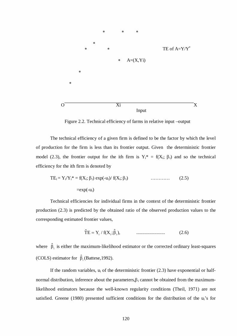
120
∗ ∗ ∗ ∗ ∗ ∗ TE of A=Y/Y∗ ∗ A=(X,Yi) ∗ ∗ O Xi X Input Figure 2.2. Technical efficiency of farms in relative input –output
The technical efficiency of a given firm is defined to be the factor by which the level
of production for the firm is less than its frontier output. Given the deterministic frontier
model (2.3), the frontier output for the ith firm is Yi* = f(Xi; βi) and so the technical
efficiency for the ith firm is denoted by
TEi = Yi/Yi* = f(Xi; βi) exp(-ui)/ f(Xi; βi) ………… (2.5)
=exp(-ui)
Technical efficiencies for individual firms in the context of the deterministic frontier
production (2.3) is predicted by the obtained ratio of the observed production values to the
corresponding estimated frontier values,
),β;f(X / YET iii= ........................ (2.6)
where iβ is either the maximum-likelihood estimator or the corrected ordinary least-squares
(COLS) estimator for iβ (Battese,1992).
If the random variables, ui of the deterministic frontier (2.3) have exponential or half-
normal distribution, inference about the parameters,βi cannot be obtained from the maximum-
likelihood estimators because the well-known regularity conditions (Theil, 1971) are not
satisfied. Greene (1980) presented sufficient conditions for the distribution of the ui’s for

121
which the maximum-livelihood estimators have the usual asymptotic properties upon which
large sample inference for the parameters, βi can be obtained. Greene (1980) proved that if
the ui’s were independent and identically distributed as gamma (γ) random variables, with
parameters γ > 2 and γ > 0, then the required regularity conditions are satisfied.
2.1.5.2 Stochastic Frontier
In a stochastic frontier production model, output is assumed to be bounded from
above by a stochastic production. Aigner, et al. (1977) and Meeusen and Broeck (1977) used
stochastic production frontier. The stochastic frontier production model incorporates a
composed error structure with a two-sided symmetric term and a one-sided component. The
one-sided components reflects inefficiency, while the two-sided error captures the random
effects outside the control of the production unit including measurement errors and other
statistical noise typical of empirical relationships. Stochastic frontiers also make it possible to
estimate standard errors and to test hypotheses, which was problematic with deterministic
frontiers because of their violation of certain maximum likelihood (ML) regularly conditions
(Schmidt, 1976). Subsequent work by Jondrow et al. (1982) provided an approach for
calculating individual firm efficiency using stochastic frontier model. A major criticism that
still afflicts stochastic frontier models is the lack of a priori justification for the selection of a
particular distributional form for the one-sided inefficiency term.
A stochastic parametric decomposition and neoclassical duality model to measure the
technical, allocative and economic efficiency of sugarcane will be measured. The stochastic
frontier production model is specified as follows:
iii εβ),f(XY += ................. (2.7)
iiii u.vβ),f(XY −+= ............... (2.8)
Where Yi is output of observation i(i.e., yield/ha), Xi denotes the actual input vector (i.e.,
input use/ha), β is the vector of production function parameters, ε is error term for
observation i.
εi = vi – ui .............. (2.9)
122
Where, v is distributed randomly and symmetrical two-sided error term that can not be
influenced by producers in represented by v (e.g., environmental factors such as temperature
and moisture): it is identically and independently distributed as N(0, σ2v) and may be
considered as the ‘normal’ error term. The u is a non-negative one-sided error term and
distributed half-normal as N(0, σ2u) which captures deviations from the frontier due to
inequality. One may note that ui measures technical inefficiency in the sense that it measures
the shortfall of output (Yi) from its maximal possible value given by the stochastic frontier
[f(Xi, β) + Vi]. Both vi and ui are independent of each other.
When a model of this form is estimated, one readily residuals β)f(XYε ii −= , which
can be regarded as estimates of the error terms εi . However the problem of decomposing
these estimates into separate estimates of the components vi and ui remained some time until
Jondrow et al. (1982) produced a method for decomposing the total error term. The
population mean and variation, of u, free of v, are estimated as:
( ) ( )2/πσuE u= ............................ (2.10)
( ) ( ) π/2πσuV 2u −= ........................... (2.11)
Given the distributional assumptions for ui and vi, the Maximum Likelihood
estimation provides sufficient information to calculate a conditional mean for u (Jondrow et
al. 1982). From this calculation, estimates of u and v may be determined. Now we can show
the conditional distribution of u given εi as presented by Jondrow et al. (1982). This
distribution contains whatever information εi yields about ui. Either the mean or the mode of
this distribution can be used as a point estimate of ui. Jondrow et al. (1982) have shown that
the assumptions made on the statistical distribution of v and u, as mentioned above make it
possible to calculate the conditional mean of u given as:
( ) ( )( )
−
−=
σλε
/σλεF1/σλεf*σ/εuE i
i
iii ................. (2.12)
Where, σ*2= σ2u.σ2
v /σ2
λ = σu / σv,

123
2v
2u σσσ +=
and f(.) and F(.) represent the standard normal density and cumulative distribution functions,
respectively, estimated at λε /σ and σ*2= σ2u .σ2
v /σ2. Thus equations (2.1) and (2.3) provide
estimates for u and v after replacing ε, σ* and λ by their estimates. When the nature of
density function for u and v is specified, the profit frontier and an error structure is estimated
using maximum likelihood techniques (Aigner et al. 1977). The λ is an indicator of the
relative variability of two sources of the error terms.
The total variance is given by:
V(ε) = V(u) +V(v) ................. (2.13)
That is, ( ) 2v
2u σ)σ
π2π(εV +
−= ............... (2.14)
Where, ( ) 2uσ
π2πuV −
= ....................... (2.15)
The deviation of the actual output to the best output, as explained by technical
inefficiency , is given by the γ parameter.
Where, )σ/(σσγ 2v
2u
2u += ...................... (2.16)
Sample technical efficiency has been estimated from frontier productions as the mean
of the difference between actual and calculated output i.e., ( ) /nYYΣ ii − ; and farm-specific
technical efficiency has been estimated as the difference between actual and calculated
output, i.e., ( )ii YY − (Kaliranjan and Shand,1985).
Although the technical efficiency of a farm associated with the deterministic and
stochastic frontier models are the same, it is important to note that they have different values
for the two models. To have a clear idea about the differences, we may consider the basic
structure of the stochastic frontier model and plot it in Figure 2.3 in which the productive
activities of two farms, represented by i and j, are considered. Farm i uses inputs with values
given by the vector of inputs (Xi) and obtains the output (Yi), but the frontier output (Yi*)

124
exceeds the value on the deterministic production function, f(Xi; βi) because its productive
activity is associated with ‘favorable’ conditions for which the random error is positive i.e.
vi> 0. in both cases, it is found that the observed production values are less than the
corresponding frontier values and the frontier values would be around the deterministic
production function associated with the farms involved. It is also evident from Figure that the
technical efficiency of farm j is greater under the stochastic frontier model than the
deterministic frontier i.e., (Yj/Yj*) > [Yj/f(Xi; βi)]. That is. j is judged technically more
efficient related to the unfavorable conditions associated with its productive activity (i.e., vj
<0) than if its production is judged relative to maximum associated value of the deterministic
function, f(Xi; βi ). How ever, for a given set of data, the estimated technical efficiency
obtained by fitting a deterministic frontier will be estimated so that no output values will
exceed it.
However, the stochastic frontier production model has the advantage over others as
the model considers the introduction of a disturbance term representing noise, measurement
error and exogenous shocks beyond the control of the production unit in addition to the
efficiency component. This avoids the over estimation of inefficiency.
The use of stochastic, parametric methodology is consistent with recent agricultural
production efficiency studies (e. g., Bravo- Ureta and Evenson, 1994; Parikh and Shah,
1994). There are also some conceptual advantages to using a stochastic approach, as it allows
for statistical noise rather than attributing all deviations to efficiency differences. Finally, this
approach is relatively straightforward to implement and interpret. The frontier production
model is estimated using Maximum Likelihood procedures. In order to empirically measure
technical efficiency, the deviations from the frontier must be separated into a random
component (i.e.,v) and an inefficiency component (i.e., u).
The Cobb-Douglas form has been used in many empirical studies, particularly those
relating to developing country agriculture. The Cobb-Douglas functional form also meets the
requirement of being self-dual, allowing an examination of economic efficiency. Schmidt and
Lovell (1979) developed a simultaneous equation cost frontier model. The corresponding cost
frontier, derived analytically, can be written in general form as

125
( )Q)P,hC = ..................... (2.17)
Where C is the minimum cost associated with the production of output Q, and P is a vector of
input prices. Applying Shephard’s lemma, we obtain
( )QP,XδPδC
ii
= ..................... (2.18)
Deterministic Production function: Y=f(xi,βi) Y∗
Output Yi
* ∗ ∗ f(Xj; βi) ∗ ∗ ∗ ∗ ∗ ∗ * ∗ ∗ ∗ * ∗ Observed output Yj
∗ Observed ∗ output Yi
O Xi Xj X Input
Figure 2.3, Technical efficiency of stochastic frontier production.
This is the system of minimum cost input demand equations. Substituting a firm’s input
prices and output quantity into the demand system in equation (2.21), we obtained the
economically efficient input vector (Xe). The Xt and X\vectors can be used to compute the
cost of the technically efficient P)(X't and the economically efficient ( )PX e
' input
combinations associated with the firm’s observed output. In addition, the cost of the firm’s
Frontier outputY* if vi>0
Frontier outputY*j if vj < 0

126
actual operating input combination is given by PX'a . These three cost measures can now be
used to compute technological (TE) and economic (EE) efficiency indexes as follows:
( ) P)/(XPXTE 'a
'p= ................... (2.19)
P)P)/(X(XEE 'a
'e= ..................... (2.20)
Finally, following Farrell (1957), the allocative efficiency (AE) index can be derived from
equations (3.19) and (3.20) as follows:
P)P)/(X(X(EE)/(TE)AE 't
'e== ................. (2.21).
Thus, the total cost or economic inefficiency of the i-th farm can be decomposed into its
technical and allocative components.
2.2. Sampling and Data Collection
2.2.1. Selection of the Samples and Sampling Techniques
In a complete enumeration, the required information is collected from each and every
element of the population. It was not be possible to interview all the sugarcane growers in the
study area due to limitation of time and resources. For this reason a reasonable size of sample
farms were chosen from the list of sugarcane farmers from a sub-zone of each the sugar mills.
Stratified proportionate random sampling technique was followed to collect information from
rural households. The stratum of the rural households was landless, small, medium and large
farmers following categories made by the Bangladesh Bureau of Statistics (BBS, 2004).
Samples were categorized on the basis of land holdings. These categories are as follows:
i) Non-farm holdings/ Landless – owning less or equal to 0.04 acres (0.02 ha) of land.
ii) Small farm holdings - owning 0.05 to 2.49 acres (0.02-1.0 ha) of land.
iii) Medium farm holdings - owning 2.50 to 7.49 acres (1.01-3.03 ha) of land.
iv) Large farm holdings - owning more than 7.50 acres (above 3.04 ha) of land.
A total of 300 rural households (100 from each district) from a comprehensive list of all
households belonging to each stratum of the study area were selected randomly.

127
Table 2.1 Number of sample in different locations and farm sizes
Locations Large farmers Medium farmers Small farmers All farmers
Rajshahi 10 (75) 51 (383) 39 (292) 100 (750) Thakurgaon 14 (67) 62 (298) 24 (115) 100 (480)
Panchagar 34 (144) 54 (230) 12 (51) 100 (425)
All 58 (286) 167 (911) 75 (458) 300 (1655) Figures in the parentheses indicate population size Source: field survey (2007-08)
2.2.2. Period of Data Collection
Based on cropping patterns, cultivation of sugarcane may be divided into two seasons –
Kharif and Rabi. The Kharif season covers from May to September and the Rabi season from
October to April. Sugarcane is all round the year crop, covering these two seasons. It is
generally planted within October to December and harvested after 12-15 months of planting.
Data and information on production technologies of sugarcane and sugarcane cropping
patterns were collected seasonally by three visits. The first visit was made just after
completion of plantation of sugarcane. Second visit was made after completion of all
intercultural operations and the last one was done after harvesting and transporting to sugar
mill. Data were collected during the most normal period of 2007-08 in the recent past by the
author herself with the help of an adequately trained assistant. Data were collected for a wider
coverage to make the analysis reasonable and realistic.
2.2.3. Data Collection Procedure and Collected Data
Required data were collected for the study from primary and secondary sources.
Regarding production aspects primary data were collected directly from the farmers by
personal interview with the help of interview schedule. In this country, usually the farmers
do not keep their records on daily and annual transactions or activities. So, it was very
difficult to collect actual data and a researcher must rely completely on the memory of the
farmers. To overcome this problem, all possible efforts was made to ensure the collection of
reasonably accurate data.
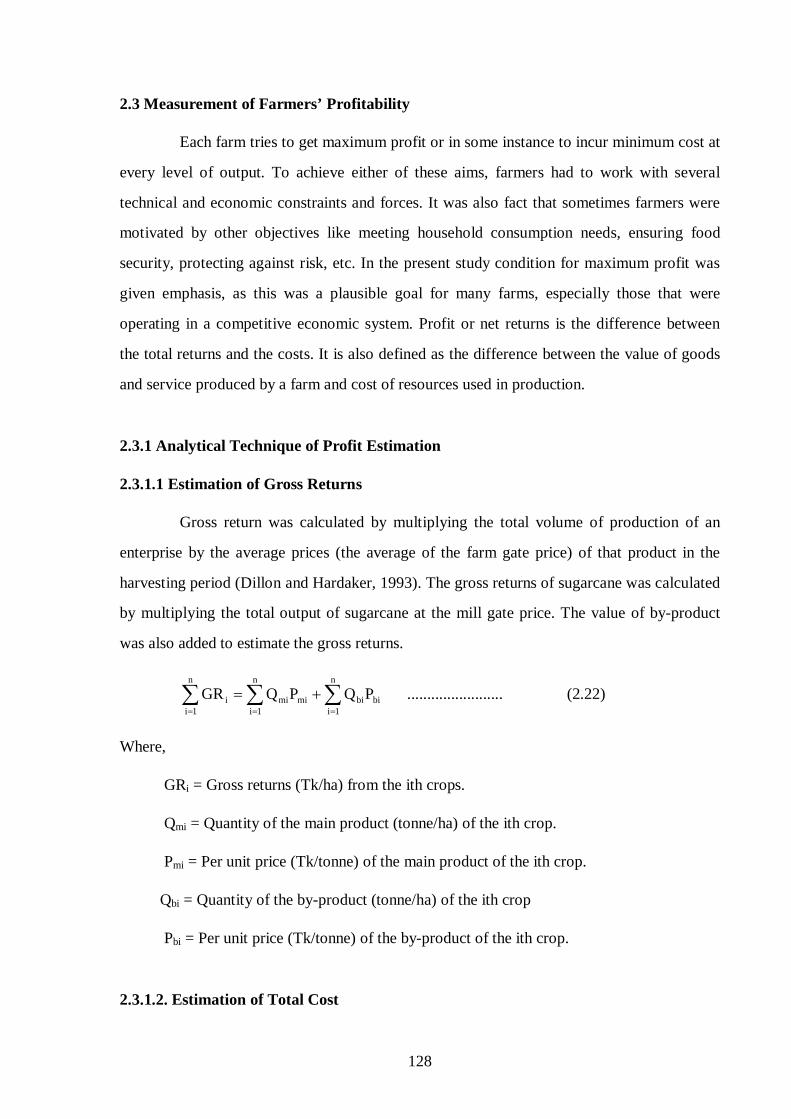
128
2.3 Measurement of Farmers’ Profitability
Each farm tries to get maximum profit or in some instance to incur minimum cost at
every level of output. To achieve either of these aims, farmers had to work with several
technical and economic constraints and forces. It was also fact that sometimes farmers were
motivated by other objectives like meeting household consumption needs, ensuring food
security, protecting against risk, etc. In the present study condition for maximum profit was
given emphasis, as this was a plausible goal for many farms, especially those that were
operating in a competitive economic system. Profit or net returns is the difference between
the total returns and the costs. It is also defined as the difference between the value of goods
and service produced by a farm and cost of resources used in production.
2.3.1 Analytical Technique of Profit Estimation
2.3.1.1 Estimation of Gross Returns
Gross return was calculated by multiplying the total volume of production of an
enterprise by the average prices (the average of the farm gate price) of that product in the
harvesting period (Dillon and Hardaker, 1993). The gross returns of sugarcane was calculated
by multiplying the total output of sugarcane at the mill gate price. The value of by-product
was also added to estimate the gross returns.
∑∑∑===
+=n
1ibibimi
n
1imi
n
1ii PQPQGR ........................ (2.22)
Where,
GRi = Gross returns (Tk/ha) from the ith crops.
Qmi = Quantity of the main product (tonne/ha) of the ith crop.
Pmi = Per unit price (Tk/tonne) of the main product of the ith crop.
Qbi = Quantity of the by-product (tonne/ha) of the ith crop
Pbi = Per unit price (Tk/tonne) of the by-product of the ith crop.
2.3.1.2. Estimation of Total Cost
129
Total cost of a product is the monetary value of all inputs used for producing that
product. In other words, it is estimated by combining market values of all inputs and services
used to produce that product. There were several types of cost items e.g., variable cost, fixed
cost, cash cost (out of pocket expenditure) etc. Total cost (TC) includes all types of variable
and fixed cost items involved in the production process. The total cost was estimated as
follows:
∑=
+=n
1iixii TFCXPTC .................................... (2.23)
Where,
TCi = Total cost (Tk/ha) of the ith crops.
Xi = quantity (kg/ha) of the ith variable.
Pxi = Per unit price (Tk/kg) of the ith variable input.
TFC = Total fixed cost of the crop.
2.3.1.3. Estimation of Profits
Farmers’ profit can be shown in two ways by (a) gross margin (GM) analysis, where
variable costs are deducted from total return, and by calculating (b) net return (NR) estimated
by deducting all costs (including fixed costs) from gross returns. Further, the case of
algebraic equation for calculating profit is as follows:
ii
n
1ii TCGR −=∏ ∑
=
.................................. (2.24)
Where,
∏i = Profit or net return (Tk/ha) of the ith crop.
GRi = Gross return (Tk/ha) of the ith crop.
TCi =Total cost (Tk/ha) of the ith crop.

130
After substituting in expressions for GRi and TCi from equations (2.22) and (2.23)
then equation (4.24) was as follows:
(a) ii
n
1i
n
1i
n
1ixibibimimi XPPQPQ(GM)∏ ∑ ∑ ∑
= = =
−+= .......................... (2.25)
(b) ∑ ∑ ∑∏= = =
+−+=n
1i
n
1i
n
1iixibibimimii
TFC)X P (P QP Q(NR) .............. (2.26)
2.4 Determination of Productive Efficiency
2. 4.1 Analytical Techniques for Productive Efficiency
2.4.1.1 Stochastic Frontier Production Function
A stochastic frontier production model was used to determine technical efficiency of
sugarcane. The stochastic production frontier model is specified as follows:
iii εβ),f(XY += .................... (2.27)
iiii u.vβ),f(XY −+= .............. (2.28)
Where, Yi was output for observation i (i.e., yield/ha), Xi denotes the actual input vector (i.e.,
input use/ha), β was the vector of production function parameters, ε was composite error term
for observation i (Aigner et al. 1977; Meeusen and Van Den Boreck, 1977) defined as:
εi = vi – ui ......................... (2.29)
Where, v was distributed randomly and symmetrical two-sided error term that can not
be influenced by producers was represented by v (e.g., environmental factors such as
temperature and moisture): it was identically and independently distributed as N (0, σ2v) and
may be considered as the ‘normal’ error term. The u was a non-negative one-sided error term
and distributed half-normal as N(0, σ2u) which captures deviations from the frontier due to
inequality. One may note that ui measures technical inefficiency in the sense that it measures
the shortfall of output (Yi) from its maximal possible value given by the stochastic frontier
[f(Xi, β) + Vi]. Both vi and ui are independent of each other.
When a model of this form is estimated, one readily gets residuals β) ,f(XYε ii −= ,
which can be regarded as estimates of the error terms εi However the problem of

131
decomposing these estimates into separate estimates of the components vi and ui remained
unresolved until Jondrow et. al. (1982) developed a method for decomposing the total error
term. The population mean and variation, of u, free of v, are estimated as:
( ) ( )2/πσuE u= ..................... (2.30)
( ) ( ) π/2πσuV 2u −= .................... (2.31)
Sample technical efficiency was estimated from frontier productions as the mean of
the difference between actual and calculated output i.e., ( ) /nYYΣ ii − ; and farm-specific
technical efficiency was estimated as the difference between actual and calculated output, i.e.,
( )ii YY − (Kaliranjan and Shand,1985).
Selecting the Functional form of the Production Function
Cobb-Douglas is a special form of the translog production function where coefficients
of the squired and interaction terms of input variables are assumed to be zero. In order best
specification for the production (Cobb-Douglas or translog) for the stochastic frontier model
using the generalized likelihood-ratio statistic “LR” defined by
LR = -2 ln[ L(H0) / L(H1)]
where, L(H0) is value of the likelihood function of the Cobb-Douglas stochastic production
frontier model, in which the parameter restrictions specified by the null hypothesis, H0 =
βji=0, (i.e. the coefficient on the squared and interaction terms of input variable are not zero).
If the null hypothesis is true, then “LR” has approximately a chi-square distribution with
degrees of freedom equal to the difference between the number of parameters estimated
under H1 and H0, respectively. We use the Cobb- Douglas and translog production function
and on the basis of the test statistic we discover that the CD is the best fit to our data set. On
the basis of this test statistic we selected the Cobb-Douglas production function. Besides this,
its coefficients directly represent the elasticity of production. The Cobb-Douglas form was
used in many empirical studies, particularly those relating to developing country in

132
agriculture. In this study, it is assumed that the Cobb- Douglas is the appropriate form of the
frontier production function
The Cobb-Douglas form was used in many empirical studies, particularly those
relating to developing country in agriculture. The empirical Cobb-Douglas frontier
production with double log form can be expressed as:
Ln Yi = β0 + β1LnX1i + β2LnX2i + β3LnX3i + β4LnX4i + β5LnX5i + β6LnX6i + β7LnX7i +
β8LnX8i + β9LnX9i + β10LnX10i + β11LnX11i + β12LnX12i + β13LnX13i + β14LnX14i +
β15LnX15i + η1D1 + η2D2 + vi – ui .................. (2.32)
Where,
Ln = Natural logarithm,
Yi = Yield of sugarcane of the ith farm (tonne/ha)
X1i = Human labour used by the ith-farm (man-days/ha)
X2i = Animal labour used by the ith-farm (pair-days/ha)
X3i = Seed used by the ith-farm (kg/ha)
X4i = Organic manure (kg/ha)
X5i = Urea used by the ith-farm (kg/ha)
X6i = TSP used by the ith-farm (kg/ha)
X7i = MP used by the ith-farm (kg/ha)
X8i = Furadan used by the ith-farm (kg/ha)
X9i = Irrigation cost used by the ith-farm (Tk/ha)
D1i = Dummy for location (1= Rajshahi, 0 = otherwise)
D2i = Dummy for location (1= Thakurgaon, 0 = otherwise)
β’s and η’s are unknown parameters to be estimated.
vi – ui = error term
2.4.1.2. Stochastic Frontier Cost Function
Schmidt and Lovell (1979) developed a simultaneous equation cost frontier model
designed to provide estimates of input-oriented technical efficiency and input allocative
efficiency. The production equation (2.27)) is the self-dual, (e.g., Cobb-Douglas functional

133
form) allowing an examination of economic efficiency. The corresponding cost frontier,
derived analytically, can be written in general form as:
( )QP,hC = ....................... (2.33)
Where, C is the minimum cost associated with the production of output Q, and P is a vector
of input prices. Applying Shephard’s lemma, we obtained
( )QP,XδPδC
ii
= ........................ (2.34)
This is the system of minimum cost input demand equations. Substituting a firm’s input
prices and output quantity into the demand system in equation (2.30), we obtained the
economically efficient input vector (Xe). The Xt and Xe vectors can be used to compute the
cost of the technically efficient P)(X't and the economically efficient ( )PX e
' input
combinations associated with the firm’s observed output. In addition, the cost of the firm’s
actual operating input combination was given by PX'a . These three cost measures were used
to compute technological (TE) and economic (EE) efficiency indexes as follows:
( ) P),/(XPXTE 'a
't= .......................... (2.35)
P)P)/(X(XEE 'a
'e= . ........................ (2.36)
Finally, allocative efficiency (AE), derived from equations (2.31) and (2.32) is given by
P)P)/(X(X(EE)/(TE)AE 't
'e== ................. (2.37)
The empirical Cobb-Douglas frontier cost function with double log form could be written
Ln Ci = α0 + α1lnP1i + α2lnP2i + α3lnP3i + α4lnP4i + α5lnP5i + α6lnP6i + α7lnP7i + α8lnP8i +
α9lnP9i + α10lnP10i + α9lnQi + vi – ui ...................... (2.38)
Where,
Ci = Minimum cost of production
Qi = Output of the ith farm(Tk./ha)
P1i = Wage rate of labour of the ith (Tk/ man-day)

134
P2i = Price of animal labour of the ith (Tk/ pair-day)
P3i = Price of seed of the ith farm (Tk/quintal)
P4i = Price of urea of the ith farm (Tk/kg)
P5i = Price of TSP of the ith farm (Tk/kg)
P6i = Price of MP of the ith farm (Tk/kg)
P7i = Price of Furadan of the ith farm (Tk/kg)
P8i = Price of organic manure of the ith farm (Tk/kg)
P9i= Price of irrigation charge of the ith farm (Tk/ha)
2.4.1.3 Technical Inefficiency Model
The ui ‘s in equation (2.32) were non negative random variables, assumed to be
independently distributed such that the technical inefficiency effect for the ith farmer, ui ,
were obtained by truncation of the normal distribution with mean zero and variance, σ2u.
Farm specific inefficiency is estimated by Jondrow et al. (1982) method that the
expected value of ui, i.e., technical inefficiency of the ith farm may be calculated by using the
distribution of conditional on total error term, i, e., (vi- ui ).
The estimating relationship is given by:
( ) ( )( )
−
−=
σλε
/σλεF1/σλεf*σ/εuE i
i
iii
= [ ]σεF(.)}{1f(.)σ i* ÷−−÷ .................... (2.39)
where, f(.) and F(.) are the standard normal density function standard normal cumulative
distribution function estimated at λεi /σ respectively. The other parameters were:
Where, σ*2= σ2u.σ2
v /σ2 ...................... (2.40)
λ = σu / σv, ...................... (2.41)
2v
2u σσσ += ....................... (2.42)
The empirical model of farm specific technical inefficiency was

135
ui = δ0 + δ1z1i + δ2z2i + δ3z3i + δ4z4i + δ5z5i + δ6z6i + δ7z7i + Wi................ (2.43)
Where,
z1i = Farm size of the ith operator (ha)
z2i = Age of the ith operator (years)
z3i = Education level of the ith operator (year of schooling)
z4i = Experience in sugarcane farming of the ith operator (years)
z5i = Household size of the ith operator (persons/household)
z6i = Dummy for extension linkage of the ith operator (1 = yes, 0 = otherwise)
z7i = Dummy for sugarcane training of the ith operator (1 = yes, 0 = otherwise)
Wi = Unobservable random variables or classical disturbance term, which were
assumed to be independently distributed, obtained by truncation of the normal distribution
with mean zero and unknown variance σ2, such that ui , is non negative.
2. 5. Growth Rates and Instability Analysis
In this section, the methodology of growth rates and instability of sugarcane with
respect to area, production and yield, factors influencing yield growth rate was discussed.
Time series data on sugarcane production, area, yield, prices of sugarcane were collected
from secondary sources like Bangladesh Bureau of Statistics (BBS) in different years,
Bangladesh Sugarcane Research Institute (BSRI), Bangladesh Sugar and Food Industry
Corporation (BSFIC), Department of Marketing (DAM), Metrological Department and other
related agencies in Bangladesh. The detailed methodologies for estimation of growth rates
were as follows:
2.5.1. Selection of the Study Area
Three districts in the Northwest of Bangladesh namely, Rajshahi, Thakurgaon and
Panchagar districts and whole Bangladesh were selected for growth rate study of sugarcane.

136
2.5.2. Data Collection Procedure and Collected Data
Time series data on sugarcane area, production, yield, price, temperature, rainfall, and
data of competing crop in the respective year were collected from secondary sources like
Bangladesh Bureau of Statistics (BBS), Bangladesh Sugarcane Research Institute (BSRI),
Bangladesh Sugar and Food Industries Corporation (BSFIC), Department of Agricultural
Extension (DAE), Department of Agricultural Marketing (DAM), Metrological Department
and other related agencies in Bangladesh. Secondary data for growth study covered the period
from 1975/76 to 2007/08 and data was collected manually from BBS census and yearbooks
of 2004 to 2008 and annual report of BFIC (2004 to 2009).
2.5.3. Analytical Techniques of Growth Rate
Any increase or decrease in the production of a crop depends basically on the changes
in area under the crop and its average yield. Measuring agricultural growth had been one of
the most extensively performed research areas. Although there were alternative methods by
which the growth rates can be calculated for a specified data series, in this study the growth
rates of area, production and yield of sugarcane was estimated by log linear function. A
simple growth model represented by the following exponential function:
btaeY = ...................... (2.44)
Where, ‘a’ and ‘b’ are parameters to be estimated, and ‘e’ is the natural exponential.
For simplicity, the error term was excluded. Because equation (2.44) is nonlinear in the
parameters, it is necessary to linearize this equation in order to apply the classical regression
model. This may be accomplished by taking the log of both sides (David, 1982);
bta lnY += ........................ (2.45)
Where,
Y = Dependent variable (production, area and yield of sugarcane, rice, wheat, potato and lentil).

137
t = Time (1975/76 to 1984/85, 1985/86 to 1994/95, 1995/96 to 2007/08 and 1975/76 to 2007/08) referred as the first, second, third and the overall period.
a = Intercept
b = Trend growth rate parameter for the period, to be estimated.
ln = natural log of the variables.
In the exponential equation b is the growth rate in ratio scale and when multiplied by
100 it represents annual percentage growth i.e. annual growth rate.
To check the significance of results t-test will also be employed. To test growth rate
following equation was followed:
Se(b)
bt = with (n-2) df. ................... (2.46)
Where, b is the growth rate, n is the number of observation and Se(b) is the standard error of
the growth.
The equation (2.44) is generally used on the consideration that the change in
agricultural output in a given year would depend upon the output in the preceding year
(Dandekar, 1980; Minhas and Vaidyanathan, 1965). It had limitation in that it assumes a
uniform rate of growth over the entire period under consideration, which may not be true in
reality. To study changes in the rate of growth, the time period is often divided into two or
more sub- periods based on some external information or arbitrarily fixed criteria (Reddy et.
al., 1998). During the whole study period, sugarcane area and production was spitted into
four sub- period e.g., period I= 1975/76 to 1984/85, period II =1985/86 to 1994/95, period III
= 1995/96 to 2007/08 and the overall period IV =1975/76 to 2007/08.
The simplest measure of instability consists of measuring percentage changes in
production (yield, acreage) from one year to another, summing these and dividing by number
of observation. Alternatively, the sum of the deviations of each observation from the mean of
the observations could be used to compute the ‘coefficient of variation’ (CV). However, both
these indices tend to overstress instability at a time of rapid growth being unable to

138
distinguish between growth and instability. This problem was overcome by computing the
C.V. from the deviations from an estimated trend line, rather than from the mean.
100XSEC.V. ×= ........................ (2.47)
Where, SE is the standered error of the estimate and X refers to the mean of observation.
Test of stability of the growth parameter:
Instability:
Instability was measured by using instability index as follows:
I= (CV)2 × (1-R2) obviously 1≤ (CV)2 ..................... (2.48)
Where,
I = Instability index.
CV = Co-efficient of variation
R2 = Co-efficient of determination.
The instability index captures both explained and unexplained variations of the
concerned variable and should better reflect the true instability situation. Besides, instability
index is effective when growth rate was high.
2. 6 Supply Response Analysis
In this section, the estimation procedure of supply response analysis of sugarcane with
respect to area, production and yield was discussed. Time series data on sugarcane area,
production, yield, prices of sugarcane and its competitive crops, rainfall, irrigated area was
collected from secondary sources like Bangladesh Bureau of Statistics (BBS) in different
years, Bangladesh Sugarcane Research Institute (BSRI), Bangladesh Sugar and Food Industry
Corporation (BSFIC), Department of Marketing (DAM), Metrological Department,
Department of Agricultural Extension (DEA) etc.. Secondary data for growth study was
covered the period from 1975/76 to 2004/05.

139
The lack of responsiveness of agricultural production to changes in price was
attributed to a number of factors which are operative in agricultural production. The historic
explanation for the disappointing response of the farmers to price incentive was that farming
is a way of life and a great part of the production is meant for self-consumption under a
subsistence form of agriculture, the individual farmers were not concerned with prices and
price relationships. However, in the modern agriculture the portion of the area of the
production is meant for the market and hence, was expected to respond to price changes. The
response to price may be low but it cannot be absent altogether.
The farmer allocates his land to different crops depending on his expected revenue
from different crops. Assuming input costs are either the same or move uniformly over time
for different crops, the expected revenue depends on expected prices and expected yields. If
yield levels were constant over time due to lack of any significant technological changes, as
was the case with sugarcane yield during the period, the acreage response equals the output
response.
2. 6.1. Analytical Techniques of Supply Response Analysis
To measure the magnitudes and nature of various supply shifters, the acreage supply
equations had been estimated with Marc Nerlove’s partial adjustment adaptive expectation
model. This model had been extensively used over the last two decades. And in spite of some
structural and estimations problems, the model is still regarded as the best available approach
for this type of study. The Nerlove’s adjustment lag model, in its simplest form, is as follows:
tt6s5y4p31t2*t10
*t VIaRaCVaCVaYaPaaA +++++++= − .............. (2.49)
t1t*t1tt Z)AB(AAA +−=− −− 0 <B <1 ...................... (2.50)
2t1t*t φ)φP(1φPP −− −+= 0 <φ <1 ..................... (2.51)
where, B and φ are the adjustment and expectation coefficients respectively.
As usual we had assumed expectations coefficients of price equal to unity and
hence 1t*t PP −= . Now substituting pt-1 for *
1tP − in equation (2.49) and consequent value of *tA
in the equation (2.50) . We obtain the following estimating equations:

140
t1t*t1tt Z)AB(AAA +−=− −−
or, t1t*t1tt Z)AB(AAA +−+= −−
= t1ttt6s5y4p31t2*t101t Z)AVIaRaCVaCVaYaPaB(aA +−++++++++ −−−
= t1ttt6s5y4p31t2*t10 ZB)(1ABBIaBRaBCVaBCVaBYaBPaBa +−++++++++ −− V
= C0 + C1Pt-1 + C2Yt-1 + C3CVp + C4CVy + C5Rs + C6It + C7At-1 +Ut .............. (2.52)
Where, C0 = a0B, C1 = a1B, C2 = a2B, C3 = a3B, C4 = a4B, C5 = a5B, C6 = a6B, C7 =1-B and Ut
=BVt + Zt .
The empirical model was
1-t9t8s7y 651-t41-t31-t2110t RIaRaCV RYaRPaPa aA aaCVaAa pt ++++++++++= −
Variables are denoted as follows:
At = Actual area planted in thousand hectares under the crop concerned which was used
dependent variables.
At-1 = Actual area planted under the crop in the previous year (lagged one year).
Pt-1 = Sugarcane price of the previous year (lagged one year).
RPt-1 = Relative price, i.e., ratio of the price of the crop concerned to the price of the
competitive crop (The competitive crops of sugarcane are wheat, maize, potato etc.,
though sugarcane is a lon duration crop, here we considered wheat-jute cropping
pattern as a competitive crop of sugarcane. The competing crop is selected keeping
in view the extent of area occupied, season and nature of crop).
RYt-1 = Relative yield, i.e., ratio of the yield of the crop concerned to the yield of the
competitive crop.
CVp = Coefficient of variation of the prices of the crop concerned for the years t-1, used as
a measure of price risk.
CVy = Coefficient of variation of the yield of the crop concerned for the years t-1 used as a
measure of yield risk.

141
Rs = Rainfall of the whole year.
It = Irrigated area under sugarcane in thousand hectares.
t = t th production period.
In the final estimated acreage supply equation, only those variables were included
which significantly increased the explanatory power of equation. We estimated the equations
using the ordinary least squares method with all variables in their log linear form. Generally
the study covered the period 1975-76 to 2007-08. The equation was estimated district wise
separately. Short-run and long-run elasticity was computed to quantify the influences of price
and non-price factors on production of sugarcane and was computed as:
For linear function,
Short-run elasticity = regression coefficient of independent variable × area ofMean
t variableindependen ofMean
While for log-linear function, the regression coefficient itself was the short run elasticity.
Long-Run Elasticity (LRE) = adjustment oft Coefficien
(SRE)elasticityrun -Short
If coefficient of adjustment is nearer to one, it indicates that the farmers had no
constraint in adjusting their acreage to the desired level in a short period. But if it is nearer to
zero, then it implies that the farmers took a long time to adjust.
Whether this model suffers from the autocorrelation problem or not, it cannot be
tested by using the DW d-statistic, since this model includes a lagged dependent variable in
the set of regressors. In the presence of a lagged dependent variable (lagged acreage for
example) in a regression equation, the DW d-statistic is likely to have reduced power and is
biased towards the value 2, Durbin (1970) and Nerlove (1958). For such an equation, Durbin
(1970) suggested an alternative test statistic known as Lagrange Multiplier Test or the h-
statistic, defined:
n.v(b)1nd)
21(1h
−−= ..................................... (2.53)
where, n = number of observations.

142
d = usual Durbin-Watson ‘d’ statistics.
v(b) is the variance of the coefficient of lagged acreage.
Under the null hypothesis of no auto-correlation, ‘h’ is asymptomatically normal with
zero mean and unit variance. The test statistic can also be used to test the hypothesis of no
serial correlation against first-order auto-correlation, even if the set of regressors in an
equation contains higher order lags of the dependent variable. However, if v(b) > 1/n, it
cannot be computed (Green, 1993).
2. 7 Yield Gap Analysis
Farm level yield of sugarcane is much lower than the yield obtained in on-station
experiment and farmers’ field demonstration. This difference is called the yield gap and it
resulted due to the variation in input use and poor management at farm level. Besides these,
there are many causes of constrains for yield gap. The concept of yield gap came from the
constraints studies carried out by the International Rice Research Institute (IRRI) which
makes a quantitative difference between experiment station yield and the actual; farm yield.
Primary data were used but research station data were used as secondary sources.
According to international Rice Research Institute (IRRI) methodology, the total yield
gap (TYG) is the difference between the potential yields (Tp – Experiment station yield) and
the actual yield (Ta – yield of sample farmers’ fields). The total yield gap (TYG) comprised
Gap I (difference between the potential yield and the potential farm yield (Yd –yield released
on the demonstration plots) and Gap II [difference the potential farm yield (demonstration
plot yield) and the actual yield]. In addition to this, various indices of yield gaps, viz., index
of yield gap [IYG = (Yp -Ya) / Yp], index of realised potential yield [IRPY = (Ya /Yp)] and
index of realized potential farm yield [IRPFY = (Ya/Yd)] were also studied.

143
Chapter 3
RESULT AND DISCUSSION
3.1 COST, RETURN AND PROFITABILITY OF SUGARCANE PRODUCTION
3.1 1. Introduction
Economic cost of a crop has important inference and can be used as tool for better
farm management and farm planning. The main focus of this chapter is to present the
production cost, return and profitability of sugarcane cultivation in the selected locations of
Bangladesh. Production cost included all kinds of fixed cost and variable costs. Total
production cost items were classified into three major groups e.g. labour costs, material costs
and miscellaneous costs. In addition to these, two indirect costs namely, interest on operating
capital and land use cost were considered to compute the total costs. Revenue was measured
by total production and its price. Profitability in sugarcane cultivation has been measured in
terms of gross margin, net return and benefit cost ratio.
3.1.2 Variable Cost of Production
Variable cost included all kinds of variable costs such as human labour, animal
labour, seed, organic manure, fertilizers, insecticides, irrigation costs etc. used for the
production of sugarcane in the study areas. Both cash expenses and imputed value of family
supplied inputs and labours were included in the variable cost.
}
3.1.2.1 Human Labour Cost
Human labour cost was the most important and the largest item of input costs. It was
required for different operations to grow sugarcane. The family labour and hired labour was
shown together in this study. Family labour includes the operator himself, the adult male and
female as well as children of a farmer’s family and the permanently hired labour. To
determine the costs of unpaid family labour, the opportunity cost concept was used. The
average wage rate was determined by the prevailing market price and it varied depending on
the season and availability of the day labour in the study area. The average computed wage
Table 3.1.1 Per hectare production cost of sugarcane

144
Particulars No./Quantity Price (Tk/unit) Total cost (Tk/ha)
Human labour (man-days/ha) 261 104.82 27358.02(34.11)
Animal labour (pair-days/ha) 23.10 190.85 4409.03(5.50)
Seed (kg/ha) 6154.10 1.18 7281.93(9.08)
Organic manure (kg/ha) 5331.10 0.40 2122.44(2.65)
Fertilizers/insecticides: 13615.18(16.97)
Urea (kg/ha) 188.34 14.11 2663.41(3.32)
TSP (kg/ha) 171.34 23.33 3998.48(4.98)
MP (kg/ha) 175 26.46 4635.34(5.78)
Furadan 5G (kg/ha) 17.4 132.91 2317.95(2.89)
Irrigation cost (Tk/ha) - - 5290.00(6.59))
Carrying cost (Tk/ha) - - 4892.00(6.10)
Total variable cost (Tk/ha) - - 64968.60(80.99)
Fixed costs :
Land use cost (Tk/ha) - - 12000(14.96)
Interest on operating capital (Tk/ha) - - 3248.43(4.05)
C. Total cost (Tk/ha) - - 80217.03(100) Source: Field survey (2007-08)
Figures in parentheses indicate percentage of total cost.
rate Tk 104.82 per- man day was used to determine the human labour cost. The average per
hectare human labour used was 261 man-days and cost was Tk 27,358.02 which shares 34.11
percent of the total cost (Table 3.1.1).Considering the location, per hectare human labour in
mandays at Rajshahi, Panchagar and Thakurgaon amounted to 272.50, 254.74 and 285
respectively (Table 3.1.2, 3.1.3, 3.1.4). The highest amount of labour cost was spent by the
farmers at Rajshahi (Tk 31,342.60/ha) followed by Panchagar (Tk 25,474.00/ha) and
Thakurgaon (Tk 28,500.00/ha). The farmers at Panchagar incurred the least amount of human
labour cost; this might be due to land preparations of some sugarcane plots were performed
by using power tiller alone whichrequired less amounts of human labour and another reason
was that wage rate was lower at Panchagar than that of Rajshahi. Human labour shared the
highest part of total production cost it was 38.24 percent at Rajshahi, 31.95 percent at
Panchagar and 36.75 percent at Thakurgaon of the total cost. Considering the farm categories,
small farmers spent more for human labour cost Tk 30,133.82/ha (36.20%) than medium Tk
26,470.23 (33.54%) and large farmers Tk 26,195.90/ha (33.07%). It implied that small
farmers employed more labour than medium and large farmers. It may be concluded that
variation in labour cost incurred by regions were due to variation in labour days and wage
rate.

145
31343
25474 28500
0
5000
10000
15000
20000
25000
30000
35000H
uman
labo
ur c
ost (
Tk/h
a)
Rajshahi Panchagar Thakurgaon
Location
26196 26470
30134
24000
25000
26000
27000
28000
29000
30000
31000
Hum
an la
bour
cos
t (Tk
/ha)
Large Medium Small
Farm categories
Figure 3.1 Human labour cost for different
locations for sugarcane cultivation Figure 3.2 Human labour cost for different farm
categories for sugarcane cultivation
Table 3.1.2 Per hectare production cost of sugarcane at Rajshahi zone
Particulars No./Quantity Price (Tk/unit) Total cost (Tk/ha)
Human labour (man-days/ha) 272.50 115 31342.80(38.24)
Animal labour (pair-days/ha) 22 180 3960.00(4.68)
Seed (kg/ha) 6138.37 1.41 8655.10(10.23)
Organic manure (kg/ha) 4142 0.40 1656.80(1.96)
Fertilizers/insecticides: 14227.98(16.82)
Urea (kg/ha) 193.94 14.42 2796.61(3.31)
TSP (kg/ha) 161.19 23.35 3763.79(4.45)
MP (kg/ha) 178.39 26.31 4693.44(5.55)
Furadan 5G (kg/ha) 26 114.39 2974.14(3.52)
Irrigation cost (Tk/ha) - - 5375.00(6.36)
Carrying cost (Tk/ha) - - 3896.00(4.61)
Total variable cost (Tk/ha) - - 69113.68(81.72)
Fixed costs :
Land use cost (Tk/ha) - - 12000.00(14.19)
Interest in operating capital (Tk/ha) - - 3455.67(4.09)
C. Total cost (Tk/ha) - - 84569.35(100) Source: Field survey (2007)
Figures in parentheses indicate percentage of total cost.

3.1.2.2 Animal Labour Cost
Animal labour was mainly used for land preparation of sugarcane cultivation. Animal
power cost included animal pair and human labour used for ploughing. The home supplied
animal labour was calculated based on the opportunity cost principle. On the other hand, the cost
of hired animal power was calculated by taking into account the prevailing market price that was
actually paid by the farmers. The wage rate of animal labour was different in different locations
in the study area. But the average wage rate of Tk 190.85 per pair day was used. On an average
per hectare animal use was 23.10 pair-days and cost was Tk 4,409.03 which shares 5.50 percent
of the total cost (Table 3.1.1). The highest cost of animal labour incurred at Rajshahi was Tk
3,960.00/ha followed by Panchagar Tk 3,819.20/ha and Thakurgaon Tk 3,700.80/ha and they
shared 4.68, 4.79 and 4.77 percent of total cost respectively (Tables 3.1.2, 3.1.3, 3.1.4).
Considering the different farm categories the highest amount of animal labour was used by large
farmers (Tk 4,803.89 /ha) followed by medium farmers (Tk 4,290.20/ha) and small farmers (Tk
4,258.54/ha). It implied that large farmers used more animal labour than medium and small
farmers.
3.1.2. 3 Seed Cost
Seed is an important factor for any crop production. Farmers normally used home
supplied seed but sometimes they purchased seeds from others. Cost of home supplied seed was
determined by the opportunity cost principle. Seed cost was found to be differing across
locations mainly due to variation in amounts of seed and planting systems. Average price of seed
was considered Tk 1.18/kg. Per hectare average seed used was 6154.10 kg (5.1 t/ha) and the cost
was Tk 7,281.93 which shares 9.08 percent of the total cost (Table 3.1.1). Considering the
location the highest amount of seed cost was incurred at Rajshahi (Tk 8655.10/ha) followed by
Panchagar (Tk 8,147.98/ha) and Thakurgaon (Tk 6,645.60/ha) which shares 10.23, 10.22 and
8.57 percent of the total cost respectively (Figure 3.5) and (Tables 3.1.2, 3.1.3 and 3.1.4).
Considering the farm categories, large farmers incurred more seed cost (Tk 7,715.66 /ha) than
medium (Tk 7,277.09/ha) and small (Tk 6,631.10) farmers (Table 3.1.5) respectively. It implied
that the large farmers spent more for seed than the medium and small farmers.

cxlvii
3960
3819
3701
3550360036503700375038003850390039504000
Cost (T
k/h
a)
Rajshahi Panchagar Thakurgaon
Locations
4804
42904259
39004000410042004300440045004600470048004900
Cos
t (T
k /h
a)
Large Medium Small
Farm categories
Figure 3.3 Animal labour cost in different
locations for sugarcane cultivation Figure 3.4 Animal labour cost of different farm
categories for sugarcane cultivation
Table 3.1.3 Per hectare production cost of sugarcane at Panchagar zone
Particulars No./Quantity Price (Tk/unit) Total cost (Tk/ha)
Human Labour (mandays/ha) 254.74 100 25474.00 (31.95)
Animal labour (pair-days/ha) 23.87 160 3819.20(4.79)
Seed (kg/ha) 5580.81 1.46 8147.98(10.22)
Organic manure (kg/ha) 5938.40 0.40 2375.36(2.98) Fertilizers/insecticides: 14055.43(17.63)
Urea (kg/ha) 182.61 13.95 2547.41(3.20)
TSP (kg/ha) 152.27 23.28 3544.85(4.45)
MP (kg/ha) 170.88 26.63 4550.53(5.71)
Furadan 5G (kg/ha) 24.31 140.38 3412.64(4.28)
Irrigation cost (Tk/ha) - - 5910.37(7.41)
Carrying cost (Tk/ha) - - 4713.00(5.91)
Total variable cost (Tk/ha) - - 64495.34(80.90) Fixed costs:
Land use cost (Tk/ha) - - 12000(15.05) Interest on operating capital (Tk/ha) - - 3224.77(4.05)
C. Total cost (Tk/ha) - - 79720.11(100) Source: Field survey (2007-08) Figures in parentheses indicate percentage of total cost.
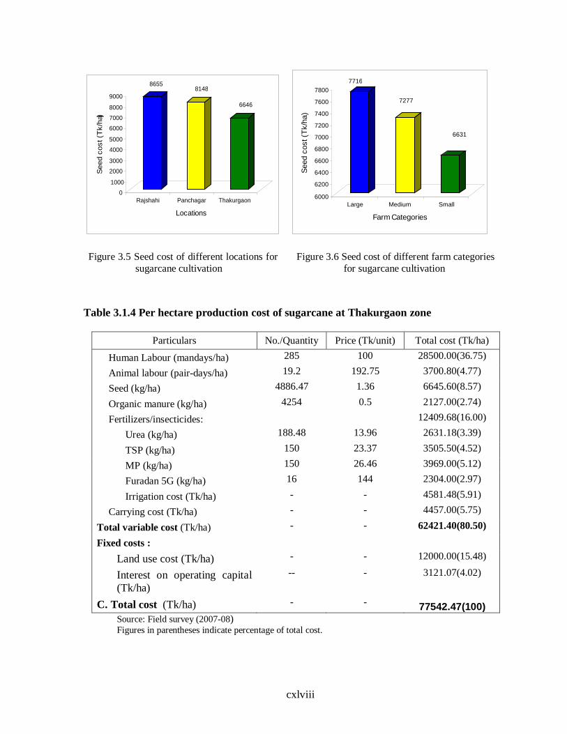
cxlviii
86558148
6646
01000
20003000
40005000
600070008000
9000S
eed
cost
(T
k/ha
)
Rajshahi Panchagar Thakurgaon
Locations
7716
7277
6631
6000
6200
6400
6600
6800
7000
7200
7400
7600
7800
Seed
cos
t (Tk
/ha)
Large Medium Small
Farm Categories
Figure 3.5 Seed cost of different locations for sugarcane cultivation
Figure 3.6 Seed cost of different farm categories for sugarcane cultivation
Table 3.1.4 Per hectare production cost of sugarcane at Thakurgaon zone
Particulars No./Quantity Price (Tk/unit) Total cost (Tk/ha)
Human Labour (mandays/ha) 285 100 28500.00(36.75)
Animal labour (pair-days/ha) 19.2 192.75 3700.80(4.77)
Seed (kg/ha) 4886.47 1.36 6645.60(8.57)
Organic manure (kg/ha) 4254 0.5 2127.00(2.74)
Fertilizers/insecticides: 12409.68(16.00)
Urea (kg/ha) 188.48 13.96 2631.18(3.39)
TSP (kg/ha) 150 23.37 3505.50(4.52)
MP (kg/ha) 150 26.46 3969.00(5.12)
Furadan 5G (kg/ha) 16 144 2304.00(2.97)
Irrigation cost (Tk/ha) - - 4581.48(5.91)
Carrying cost (Tk/ha) - - 4457.00(5.75)
Total variable cost (Tk/ha) - - 62421.40(80.50)
Fixed costs :
Land use cost (Tk/ha) - - 12000.00(15.48)
Interest on operating capital (Tk/ha)
-- - 3121.07(4.02)
C. Total cost (Tk/ha) - - 77542.47(100) Source: Field survey (2007-08)
Figures in parentheses indicate percentage of total cost.

cxlix
. 3.1.2.4 Organic Manure Cost
Organic manure is an important factor for agricultural production. The farmers usually used
home supplied organic manure and a few farmers purchased it. Farmers used cow-dung and ash
as manure. The value of the home supplied and purchased cow-dung and ashes were calculated
at the prevailing market price. Average market price of organic manure was estimated Tk 0.40
per kg. On an average per hectare organic manure cost was Tk 2,122.44 which shares 2.65
percent of the total cost (Table 3.1.1). Considering the different locations the highest organic
manure cost was incurred at Thakurgaon (Tk 2,127 /ha) followed by Panchagar (Tk 2,375/ha)
and at Rajshahi (Tk 1656.80/ha). Within the different farm size groups the large farmers spent
highest per hectare organic manure cost of Tk 3,201.61 followed by medium farmers (Tk
2,007.16) and small farmers (Tk 1,770.45) respectively. It implied that the large farmers spent
more money for organic manure than the medium and small farmers.
3.1.2.5 Fertilizer and Insecticide Cost
Fertilizer is a major prerequisite input of crop production. The farmers mainly used
fertilizers as urea, TSP, MP and gypsum in sugarcane production and as insecticides they used
Furadan 5G and Regent 3 GR. Fertilizer and insecticides costs were charged according to the
actual price paid by the farmers. However, the average prices per kg paid by the farmers were Tk
14.11, Tk 23.33, Tk 26.046 and Tk 132.91 for urea, TSP, MP and Furadan 5G respectively
which were taken into consideration for calculation of cost of fertilizers and insecticides. On
average farmers spent per hectare Tk 13,615.18 for fertilizer and insecticides cost in sugarcane
production. In terms of different location, the highest amount of Taka 14,227.98 was spent by
farmers at Rajshahi followed by the farmers at Panchagar (Tk 14,055.43) and Thakurgaon (Tk
12,409.68) for fertilizers and insecticides use. Fertilizer and insecticides combined constituted
about 16.97 percent of the total cost of production with 17.63 percent at Panchagar, 16.82
percent at Rajshahi and 17.65 percent at Thakurgaon. Considering the farm categories, the large
farmers spent more for fertilizers and insecticides cost (Tk 13,925.40/ha) than medium (Tk
13,793.04) and small farmers (Tk 12905.24). This may be due to the more ability of the large
category of farmers.

cl
3.1.2.6 Irrigation Cost
Almost all farmers used irrigation water for sugarcane cultivation. Most farmers used
their own shallow tube-well (STW), and some farmers hired from others. The cost of irrigation
included the rental charge of machine plus the costs of fuel. Some farmers rented/borrowed only
water from the STW owners by paying some charge. On an average per hectare irrigation cost
was Tk 5,290.00 (Table 3.1.1). Comparatively higher amounts were spent by the farmers at
Panchagar (Tk 5,910.37/ha) followed by Rajshahi (Tk 5,375.00/ha) and Thakurgaon (Tk
4,581.48/ha) for irrigation cost. The farmers at Thakurgaon incurred least cost for irrigation. This
is because on an average they applied less irrigation than other locations. On an average the
irrigation cost constituted about 6.59 percent of total cost of production with the highest 7.41
percent at Panchagar and the lowest 5.91 percent at Thakurgaon (Tables 3.1.1, and Table 3.1.5).
Viewed from farm categories, the large farmers spent the highest irrigation cost (Tk 5,278.51/ha)
followed by medium (Tk 5,271.69) and small farmers (Tk 5,183.17/ha). This may be due to more
ability of larger categories of farmers. Similar trend was observed in different locations and farm
categories within the locations.
3.1.2.7 Carrying cost
The cost of marketing in the case of sugarcane involved mainly the cost of carrying the canes
from farms to procurement centre/ millgate. Sugarcane growers transported their canes to
procurement centre by bullock or buffalo carts or tractor. On average per hectare carrying cost
was Tk. 4,892 .00 which shares 6.10 percent of the total cost (Table 3.1.1).
3.1.3 Fixed Cost of Sugarcane Production
3.1.3.1 Land Use cost
In the study area, the land use cost per hectare differed from plot to plot depending on the
location, fertility, topography and crop production facilities of the land. In calculating land use
cost, the average rental value of land per hectare for a particular year as reported by farmers was
considered. The average land use cost was calculated at Tk. 12,000 per hectare.

cli
3.1.3.2 Interest on Operating Capital
Interest on operating capital involved all costs excluding those for which interest had
already been charged. Interest on operating capital was charged at the prevailing bank interest. If
the farmers borrow money from the bank they must pay interest at the same rate. In this study, 10
percent rate of interest per annum was considered. For calculating interest on operating capital
the following formula was used:
Interest on operating capital = 2
period timeofLength interest of Ratecost Operating ××
This actually represented the average operating costs over the period because all costs were not
incurred at the beginning or at any fixed time. The cost was estimated for a period of 12 months.
Per hectare interest cost in sugarcane production was Tk. 3248.43 which shares 4.04 percent of
the total cost.
3.1.4 Total Cost of Production
Total cost of production included all variable and fixed costs. On an average, total cost of
production for sugarcane cultivation was Tk. 80,217.03 per hectare of which 80.99 percent was
shared by variable cost, 14.96 percent by land use cost and 4.05 percent by interest in operating
capital cost (Table 3.1.1). Within the total cost human labour shared the highest percent of the
total cost (34.11%) followed by fertilizers & insecticides cost (16.97%), land use cost (14.96),
seed cost (9.08%), Irrigation (6.59%), Carrying cost (6.10%) and animal labour cost (5.50%).
The shares of the inputs within the total cost were shown in figure 3.13.
The highest production cost was incurred by the farmers at Rajshahi (Tk. 84,569.35/ha)
followed by those at Thakurgaon (Tk.79,720.11/ha) and Panchagar (Tk. 77,542.47/ha) (Figure
3.14). Considering the average level of farm categories the highest production cost was incurred
by small farmers (Tk. 83,247.17 /ha) followed by large (Tk. 79,222.02/ha) and medium farmers
(Tk. 78,915.88/ha) (Table 3.1.6 and Figure 3.15). This was because, the small farmers used
higher amount of human labour from themselves.

clii
1657
23752127
0
500
1000
1500
2000
2500
Cos
t /ha
Rajshahi Panchagar Thakurgaon
Locations
3202
20071770
0
500
1000
1500
2000
2500
3000
3500
Cos
t /ha
Large Medium Small
Farm Categories
Figure 3.7 Organic manure cost of different locations for sugarcane cultivation
Figure 3.8 Organic manure cost of different farm categories for sugarcane cultivation
1422814055
12410
11500
12000
12500
13000
13500
14000
14500
Cost
(Tk/h
a)
Rajshahi Panchagar Thakuraon
Locations
1392513793
12905
12200
12400
12600
12800
13000
13200
13400
13600
13800
14000Co
st (T
k/ha
)
Large Medium Small
Farm Categories
Figure 3.9 Fertilizers and insecticides cost in
different locations for sugarcane cultivation
Figure 3.10 Fertilizers and insecticides cost for different farm categories for sugarcane cultivation

cliii
53755910
4581
0
1000
2000
3000
4000
5000
6000
Cost
(Tk/h
a)
Rajshahi Panchagar Thakurgaon
Locations
5279 5271
4999
4850
4900
4950
5000
5050
5100
5150
5200
5250
5300
Cost
(Tk
/ha)
Large Medium Small
Farm categories
Figure 3.11 Irrigation cost for sugarcane
cultivation in different locations Figure 3.12 Irrigation cost for different farm
categories for sugarcane cultivation Table 3.1.5 Per hectare production cost of sugarcane in different locations (Tk)
Particulars Rajshshi Panchagar Thakurgaon Human Labour 31342.80(38.24) 25474.00 (31.95) 28500.00(36.75) Animal labour 3960.00(4.68) 3819.20(4.79) 3700.80(4.77) Seed 8655.10(10.23) 8147.98(10.22) 6645.60(8.57) Organic manure 1656.80(1.96) 2375.36(2.98) 2127.00(2.74) Fertilizers/Insecticides: 14227.98(16.82) 14055.43(17.63) 12409.68(16.00)
Urea 2796.61(3.31) 2547.41(3.20) 2631.18(3.39) TSP 3763.79(4.45) 3544.85(4.45) 3505.50(4.52) MP 4693.44(5.55) 4550.53(5.71) 3969.00(5.12) Furadan 5G 2974.14(3.52) 3412.64(4.28) 2304.00(2.97) Irrigation cost 5375.00(6.36) 5910.37(7.41) 4581.48(5.91)
Carrying cost 3896.00(4.61) 4713.00(5.91) 4457.00(5.75) Total variable cost 69113.68(81.72) 64495.34(80.90) 62421.40(80.50) Fixed cost :
Land use cost 12000.00(14.19) 12000(15.05) 12000.00(15.48) Interest in operating capital
3455.67(4.09) 3224.77(4.05) 3121.07(4.02)
C. Total cost 84569.35(100) 79720.11(100) 77542.47(100) Sources: Compiled from Table no. 3.1.2, 3.1.3 and 3.1.4

cliv
Table 3.1.6 Per hectare sugarcane production cost by different farm size groups (Tk)
Particulars Large Medium Small All Human Labour 26195.90(33.07) 26470.23(33.54) 30133.82(36.20) 27599.98(34.30) Animal labour 4803.89(6.06) 4290.20(5.44) 4258.54(5.12) 4407.63(5.48) Seed 7715.66(9.74) 7277.09(9.22) 6631.10(7.97) 7272.06(9.04) Organic manure 3201.61(4.04) 2007.16(2.54) 1770.45(2.13) 2326.41(2.89) Fertilizers/Insecticides: 13925.40(17.58) 13793.04(17.48) 12905.24(15.50) 13541.23(16.83)
Urea 2699.02(3.41) 2636.07(3.34) 2680.79(3.22) 2671.96(3.32) TSP 4441.98(5.61) 4029.84(5.11) 3637.62(4.37) 4036.48(5.02) MP 4588.83(5.79) 4706.66(5.96) 4494.052(5.40) 4596(5.71) Furadan 5G 2195.57(2.77) 2420.47(3.07) 2092.78(2.51) 2236.27(2.78) Irrigation cost 5278.51(6.66) 5271.69(6.64) 4999.30(6.01) 5183.17(644)
Carrying cost 5500.00(6.94) 4620.00(5.85) 4556.00(5.47) 4892(6.08)
Total variable cost 64020.97(80.81) 63729.41(80.76) 67854.45(81.51) 65201.61(81.03)
Fixed cost :
Land use cost 12000.00(15.15) 12000.00(15.21) 12000.00(14.41) 12000.00(14.91) Interest in operating capital
3201.05(4.04) 3186.47(4.04) 3392.72(4.08) 3260.08(4.05)
C. Total cost 79222.02(100) 78915.88(100) 83247.17(100) 80461.69(100) Source: Field survey (2007-08)
Figures in parentheses indicate percentage of total cost.
6.59
6.1
14.96
34.11
5.59.082.65
16.97
Humanlabour
Animal. labour
Seed
Organic manure
Fertilizers &insecticides
Irrigation
Carrying
Others
Figure 3.13 Percent shares of different inputs cost in sugarcane production

clv
79,22278,916
83247
76,00077,00078,00079,00080,00081,000
82,00083,00084,000
Prod
uctio
n co
st(T
k/ha
)
Large Medium Small
Farm categories
84,569
79,720
77,542
74,000
76,000
78,000
80,000
82,000
84,000
86,000
Prod
uctio
n co
st (T
k/ha
)
Rajshahi Panchagar Thakurgaon
Locations
Figure 3.14 Total production cost at different
locations for sugarcane cultivation Figure 3.15 Total production cost of different
farm categories for sugarcane cultivation
3.1. 5 Yield and Gross Returns of Sugarcane Production
An average per hectare yield of sugarcane was 58.53 t/ha. The highest yield was obtained
at Rajshahi (62.30 t/ha) followed by Panchagar (57.80 t /ha) and Thakurgaon (55.80 t/ha) (Table
3.1.7). Considering the farm categories, the large farmers obtained the highest yield 59.83 t/ha
followed by medium farmers 59.09 t/ha and small farmers 56.67 t/ha (Table 3.1.8). On the other
hand, the farmers earned a large volume of by-products. It is very difficult to estimate the value
of by-products and in most cases the guess of estimation of farmers was used for valuing the by-
products. However, the average value of by-products at Rajshahi, Panchagar and Thakurgaon
was Tk 8,721.36, Tk 8,570.03 and Tk 7,300.00 per hectare respectively. When farm categories
were considered, the large, medium and small farmers obtained the by-products amounting Tk
7,438.02, Tk 8,114.80 and Tk 9,514.80 per hectare respectively. Gross return from sugarcane
cultivation included return from main cane and by-product, mutha, green leaves, dry leaves etc.
On an average the gross return from sugarcane production was Tk 98,492.07 per hectare (Table
3.1.8). The highest gross return was obtained by the farmers at Rajshahi ( Tk 1,04,663.36/ha)
followed by those at Panchagar (Tk 97,582.03/ha) and Thakurgaon (Tk 93,232.00) (Table 3.1.7).
The gross return was found to vary among locations mainly due to variation in yield which was
caused by the differences in the levels of input use.

clvi
Considering the average level of farm categories there were not much differences in gross
return among different farm size groups. The gross returns of large, medium and small farmers
were Tk 99,576.22/ha, Tk 99,113.40/ha and Tk 96,786.60/ha respectively (Table 3.1.8). The
study was designed to provide a wider coverage and farm size was considered as a basis of
desegregation. The costs and returns depend on many factors across regions and farm sizes. It is
neither possible nor desirable to clearly detect the profitability by farm size or by regions.
3.1.6 Net Returns of Sugarcane Production
Net return was determined by deducting all costs from gross return. The average net
return was Tk 18,030.38 per hectare which varied from Tk 13,539.43 to Tk 20,354.20 per
hectare for small and large farms (Table 3.1.7). The highest net return was found with the
farmers at Rajshahi, (Tk 20,094.01/ha) followed by that at Panchagar (Tk 17,861.92/ha) and
Thakurgaon (Tk 15,689.53/ha) (Table 3.1.6). Within the farm categories the large farmers
obtained the highest net returns (Tk 20,354.20/ha) followed by medium (Tk 20,197/ha) and small
(Tk 13,539.43/ha).
3.1.7 Benefit Cost Ratio (BCR)
Benefit cost ratio (undiscounted) for sugarcane was calculated as a ratio of gross return to
the total cost. Benefit cost ratio (BCR) considering total cost of production is presented in Table
3.1.7. It was observed that overall BCR considering the total cost was 1.22 which varied from
1.16 to 1.26 in different farm categories, the highest being with the large farmers. This indicated
that the large farmers earned comparatively higher net return from sugarcane cultivation
compared to medium and small farmers. Among the locations, the higher BCR considering total
cost was found with the farmers at Rajshahi (1.24) followed by Panchagar (1.22) and
Thakurgaon (1.20) (Figure 3.18).

clvii
Table 3.1.7 Total cost, gross return and net return at different locations
Particulars Different Locations
Rajshahi Panchagar Thakurgaon
Yield(t/ha) 62.30 57.80 55.80
Value of output (Tk/ha) 95942.00 89012.00 85932.00
Value of By-Products Tk/ha 8721.36 8570.03 7300.00
Gross Return (Tk/ha) 104663.36 97582.03 93232.00
Total cost (Tk/ha) 84569.35 79720.11 77542.47
Net Return(Tk/ha) 20094.01 17861.92 15689.53
Benefit cost Ratio(BCR) 1.24 1.22 1.20
Source: Field survey (2007-08)
Table 3.1.8 Total cost, gross return and net return of different farm categories
Particulars Different Farm Categories
Large Medium Small All
Yield (t/ha) 59.83 59.09 56.67 58.53
Value of output (Tk/ha) 92138.20 90998.60 87271.80 90136.20
Value of By-Products(Tk/ha) 7438.02 8114.80 9514.80 8355.87
Gross Return (Tk/ha) 99576.22 99113.40 96786.60 98492.07
Total cost (Tk/ha) 79222.02 78915.88 83247.17 80461.69
Net Return(Tk/ha) 20354.20 20197.52 13539.43 18030.38
Benefit cost Ratio(BCR) 1.26 1.25 1.16 1.22 Source: Field survey (2007-08)

clviii
104663
84569
20094
97582
79720
17862
93232
77542
15689
0
20000
40000
60000
80000
100000
120000
Cost
and
retu
rn (T
k/ha
)
Rajshahi Panchagar Thakurgaon
Location
Gross return Total cost Net returns
Figure 3.16 Gross return, total cost and net returns at different locations
99576
79222
20354
99113
78916
20198
96787
83247
13539
0
20000
40000
60000
80000
100000
Cost
and
retu
rns
(Tk/
ha)
Large Medium Small
Farm Categories
Gross return Total cost Net returns
Figure 3.17 Gross return, total cost and net returns at different farm categories
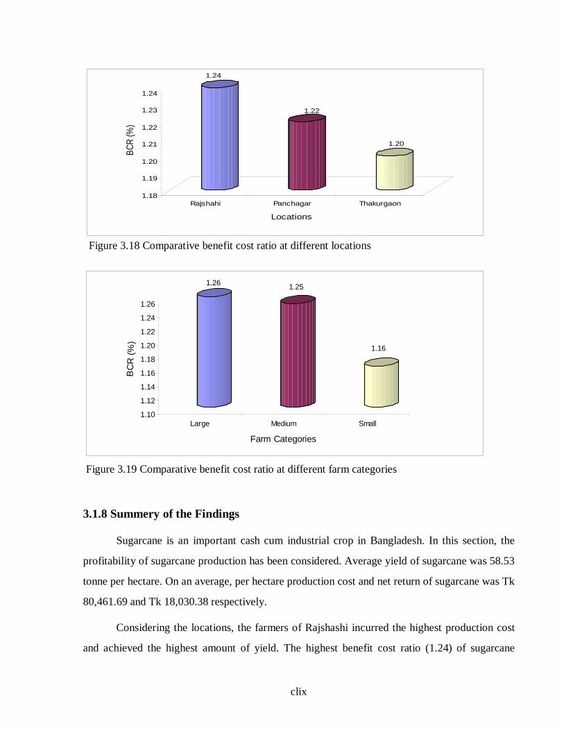
clix
1.24
1.22
1.20
1.18
1.19
1.20
1.21
1.22
1.23
1.24
BCR
(%)
Rajshahi Panchagar Thakurgaon
Locations
Figure 3.18 Comparative benefit cost ratio at different locations
1.26 1.25
1.16
1.10
1.12
1.14
1.16
1.18
1.20
1.22
1.24
1.26
BC
R (%
)
Large Medium Small
Farm Categories
Figure 3.19 Comparative benefit cost ratio at different farm categories
3.1.8 Summery of the Findings
Sugarcane is an important cash cum industrial crop in Bangladesh. In this section, the
profitability of sugarcane production has been considered. Average yield of sugarcane was 58.53
tonne per hectare. On an average, per hectare production cost and net return of sugarcane was Tk
80,461.69 and Tk 18,030.38 respectively.
Considering the locations, the farmers of Rajshashi incurred the highest production cost
and achieved the highest amount of yield. The highest benefit cost ratio (1.24) of sugarcane

clx
production achieved by the farmers of Rajshahi. According to farm categories the highest
production cost incurred by small farmers (Tk 83,247.7/ha) followed by large (Tk 79,222.02/ha)
and medium farmers (Tk 78,95.88/ha). The small farmers used themselves as agricultural labour
in production but they could not use required amount of other inputs for their financial condition.
Thus the productivity was declined. On the other hand, the large farmers used hired labour
according to requirements and used higher input costs. As a result, the large farmers got the
highest yield (59.83 t/ha) and thereby the highest net return (Tk 20,354.20/ha) followed by
medium and small farmers.
Sugarcane is a long duration crop and requires high cost to grow. Every farmer wants to
get more return from their investment within short period. So, especially for the poor farmers it is
difficult to wait for such a long time. Moreover, due to the increasing demand of cereal and
vegetables crops, now the cultivation of sugarcane is decreased gradually. Therefore, the
sustainability of long duration sugarcane is now at threat. However, to combat the declining of
sugarcane area, intercropping is one of the ways for increasing productivity and economic
profitability from per unit area. Systematic, intercropping in sugarcane with various short
duration crops like potato, cabbage, onion, lentil, mungbean etc. has been proven profitable in
comparison to growing sugarcane as sole crop (Yadva and Verma, 1984, Alam et al., 2007;
Kabir et al. 2004(Appendix-B). It is reported that in Mauritius, about 70 - 77 percent cane areas
are intercropped mainly with potato and tomato (Imam, 1990). However, in our country the
adoption rate of intercropping with sugarcane is still low and it ranges 20-30 percent so far
(Anon. 2009). Therefore, there is an ample scope to increase productivity by introducing
intercrop systematically.
To increase productivity it is essential to estimate productive efficiency. Efficiency is an
important issue of productivity growth in the agriculture based economy of developing countries.
Therefore, after estimating profitability it is essential to determine the productive efficiency of
sugarcane production.
clxi
3.2 EFFICIENCY AND DETERMINANTS OF EFFICIENCY IN SUGARCANE PRODUCTION
3.2.1. Introduction
The concept of efficiency is at the core of economic theory. The theory of production
economics is concerned with optimization and optimization implies efficiency. Efficiency is an
important issue of productivity growth in the agriculture based economy of developing countries.
The crucial role of efficiency in increasing agricultural output has been widely recognized by
researchers and policy makers alike. The estimation of efficiency with the help of production
function has been a popular area of applied econometrics. Recent works in duality theory, which
has linked production and cost function, has made this topic more attractive. However, definition
of a technical efficiency reflects the ability of a farm to obtain the maximum possible output
from a given level of inputs and production technology. It is a relative concept, since each farm’s
production performance is compared to a best- practice input-output relationship or production
frontier. A farm is technically inefficient in the sense that if it fails to produce maximum output
from a given level of input. Technical inefficiency is then measured as the deviation of an
individual farm from the best-practice frontier. Economic efficiency reflects the minimum cost
of producing a given level of output at the same set of input prices. Estimates on the extent of
efficiency may help improve productivity through input reallocation or cost minimization. The
main objective of this chapter is to estimate the technical, allocative and economic efficiencies as
well as frequency distribution of different level of sugarcane farmers.
The technical efficiency in production was estimated by using the stochastic frontier
production. The primary advantage of a stochastic frontier production function is that it enables
one to estimate Ui (non-negative random variable which is under the control of the farm) and
therefore also to estimate farm specific technical efficiencies. The measure of technical
efficiency is equivalent to the ratio of the production of the ith farm to the corresponding
production value if the farm effect Ui were zero.

clxii
3.2.2 Maximum Likelihood Estimates of Farm-specific Stochastic Frontier Production Function and Inefficiency Model
The maximum likelihood estimates (MLE) methods of the parameters of the stochastic
production frontier were obtained using the programme, computer software, FRONTIER 4.1
(Coelli, 1996). Asides from estimates of coefficients in the model, the output also provides other
variance parameters such as sigma squared (σ2), gama (γ) and log likelihood function. To
estimate the farm specific technical efficiency for sugarcane production in the study area, yield
as dependent variable and other independent variables were standardized on the basis of per
hectare of land. The maximum likelihood estimates for the parameters of the Cobb-Douglas
stochastic frontier production function for the sugarcane farmers are presented Table 3.2.1.
In this study to estimate farm specific technical efficiency for sugarcane production, the
stochastic frontier production function was used. The empirical results indicated that the
coefficients of human labour, animal labour, seed, urea, Furadan 5G and irrigation cost were
positive and significant, while that of organic manure, TSP and MP were positive but not
significant.
At 1% level of significance, the coefficients of human labour, seed, urea, Furadan 5G and
irrigation costs were positive. In other words the elasticity of human labour, seed, urea, Furadan
5G and irrigation cost were 0.264, 0.139, 0.168, 0.023 and 0.013 respectively. It implied that
human labour, seed, urea, Furadan 5G and irrigation cost had significant and positive impact on
sugarcane production. The yield of sugarcane would increase by 0.264, 0.139, 0.168, 0.023 and
0.013 percent if the farmers apply 1 percent additional human labour, seed, urea, Furadan 5G and
irrigation cost respectively. Moreover, the coefficient of dummy variables D2 (Rajshahi =1 and
others =0) was found positive and significant at 1 % level. This implied that sugarcane
production is higher in Rajshahi than in other locations. This is because the farmers of Rajshahi
location are more efficient and advanced in sugarcane production than farmers of other locations
and got highest BCR (Table 3.1.6). On the other hand the dummy variable D1 of Thakurgaon
location was negative and significant. This implied that the farmers of Thakurgaon were not
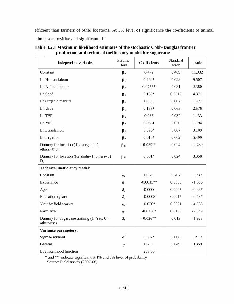
clxiii
efficient than farmers of other locations. At 5% level of significance the coefficients of animal
labour was positive and significant. It
Table 3.2.1 Maximum likelihood estimates of the stochastic Cobb-Douglas frontier production and technical inefficiency model for sugarcane
[ [[ Independent variables Parame-
ters Coefficients Standard error t-ratio
Constant β0 6.472 0.469 11.932
Ln Human labour β1 0.264* 0.028 9.507
Ln Animal labour β2 0.075** 0.031 2.380
Ln Seed β3 0.139* 0.0317 4.371
Ln Organic manure β4 0.003 0.002 1.427
Ln Urea β5 0.168* 0.065 2.576
Ln TSP β6 0.036 0.032 1.133
Ln MP β7 0.0531 0.030 1.794
Ln Furadan 5G β8 0.023* 0.007 3.109
Ln Irrgation β9 0.013* 0.002 5.499
Dummy for location (Thakurgaon=1, others=0)D1
β10 -0.059** 0.024 -2.460
Dummy for location (Rajshahi=1, others=0) D2
β11 0.081* 0.024 3.358
Technical inefficiency model:
Constant δ0 0.329 0.267 1.232
Experience δ1 -0.0013** 0.0008 -1.606
Age δ2 -0.0006 0.0007 -0.837
Education (year) δ3 -0.0008 0.0017 -0.487
Visit by field worker δ4 -0.030* 0.0071 -4.233
Farm size δ5 -0.0256* 0.0100 -2.549
Dummy for sugarcane training (1=Yes, 0= otherwise)
δ6 -0.026** 0.013 -1.925
Variance parameters :
Sigma- squared σ2 0.097* 0.008 12.12
Gamma γ 0.233 0.649 0.359
Log likelihood function 269.85 * and ** indicate significant at 1% and 5% level of probability Source: Field survey (2007-08)

clxiv
indicates that the elasticity of animal labour was 0.075, which was playing a significant positive
role on sugarcane production. It further implied that holding other things remaining same, the
yield of sugarcane would increase by 0.075 percent as farmers would apply 1 percent additional
animal labour.
The coefficients of the explanatory variable in the model for the inefficiency effects,
defined by equation 2.43, were of particular interest to this study. The coefficient for the
experience was negative and significant, which implied that the inefficiency effects decrease
with the increase of the experiences of farm operators of sugarcane. In other words, technical
efficiency increased with the increase of experiences of the farmers. The farmers, who had
greater experience about sugarcane production, were technically more efficient than less
experienced ones in managing and allocating productive resources. This result conforms to result
of similar studies (Sumi et al. 2004). The coefficients for the age variable was 0.006 and
negative too, but it is non- significant so it can not be said with emphasis that older farmers are
technically less inefficient than the younger farmers. It can be said, however, that with the
increase of age of farmers the efficiency of farmers tends to increases. This result is in line with
those of Rao et al. (2003), Hussain (1999) and Coelli (1996). According to them the negative
coefficients suggest that as the age, education increases, the inefficiency decreases. The
coefficient for the education variable was negative, which indicates that the farmers with greater
years of formal schooling tend to be more technically efficient. This indicates that the farmers
with more education respond more readily in using the new
technology and produce output closer to the frontier. This result is similar to that of Seyoum et
al. 1998; Dey, et al. 2000; Pagan, 2001. The coefficient for the visit by the field worker was 0.03
and negative at one percent level of significance. This implied that the regular visit by field
workers to the farmers’ sugarcane plot tends to decrease inefficiency or increase efficiency. This
is similar to that of Rahman et al. (2000), Chaudhry (2001), and Islam (2003). The estimated
coefficient of the farm size variable is 0 .026 and negative at five percent level of significance,
which indicated that the increase of sugarcane farm size tends to decrease inefficiency or
increase efficiency. This is similar to that of Rahman et al. (2000), Ahmed et al. (2002). Training
improves skills and the result supports that professional training reduces inefficiency. The

clxv
coefficient of sugarcane training (Dt) was negative and significant at 5% level. It indicated that
the training on sugarcane production reduced the production inefficiency and increased the
technical efficiencies of sugarcane production. If a farmer gets more training programmes, his
level of inefficiencies would decrease. The estimated values of the variance parameters (σ and γ )
were large and significantly different from zero, which indicated a good fit and correctness of the
specified distributional assumption.
3.2.3 Maximum Likelihood Estimates of Location-specific Stochastic Frontier Production Function and Inefficiency Model
Estimation of location specific technical efficiency for sugarcane is essential for drawing
appropriate policy for the location. If we find out the significance of efficiency differences
between locations then we will be able to identify the factors which are responsible for those
differences. The maximum likelihood estimates of the coefficients of location specific stochastic
Cobb- Douglas production frontier and technical inefficiency model is shown in Table 3.2.2.
The empirical result indicated that at Rajshahi, the coefficients of human labour, organic
manure, urea, MP, Furadan 5G and irrigation costs were positive and significant, while that of
animal labour, seed, TSP cost was positive but not significant. It indicated that human labour,
organic manure, urea, MP, Furadan 5G and irrigation costs had significant and positive impacts
on sugarcane production at Rajshahi.
At 1% level of significance human labour had the largest positive coefficient compared to
other inputs. In other words, the elasticity of human labour (0.42) was the biggest amount than
all other inputs at Rajshahi. Holding other things constant, the yield of sugarcane would increase
by 0.415% as farmers used 1% additional human labour in different types of management
practices like, weeding, mulching, properly fertilizer application, insect and pest control
(mechanical control by hand), tying, etc. At 1% level of significance, the coefficients of organic
manure (0.012), MP (0.102), Furadan 5G (0.022) and irrigation cost (0.011) were positive
implying that holding other things constant, the yield of sugarcane at Rajshahi would increase by
0.0120, 0.102, 0.022 and 0.01 percent as farmers increase 1% additional organic manure, MP,

clxvi
Furadan 5G and irrigation cost respectively. The coefficient of urea (0.167) was significant at 5%
level, implying that holding other things
Table 3.2.2 Maximum likelihood estimates for parameters of location-specific Cobb-Douglas stochastic frontier production and technical inefficiency model for sugarcane
Independent variables Parameters Locations
Rajshahi Thakurgaon Panchagar
Constant β0 6.845 (0.762) 6.709 (0.741) 4.872(0.979)
Ln Human labour β1 0.415* (0.040) 0.222* (0.041) 0.299*(0.053)
Ln Animal labour β2 0.002 (0.069) 0.087 (0.053) 0.029(0.045)
Ln Seed β3 0.035 (0.095) 0.172* (0.062) 0.148*(0.038)
Ln Organic manure β4 0.012* (0.002) 0.005 (0.004) 0.082*(0.024)
Ln Urea β5 0.167** (0.082) 0.139* (0.052) 0.026(0.167)
Ln TSP β6 0.072 (0.042) 0.008 (0.054) 0.033(0.043)
Ln MP β7 0.102* (0.023) 0.145* (0.053) 0.059(0.044)
Ln Furadan 5G β8 0.022* (0.007) - 0.005 (0.025) 0.021(0.026)
Ln Irrgation β9 0.011* (0.002) 0.017** (0.008) 0.025*(0.004)
Technical inefficiency model:
Constant δ0 0.512 (0.301) 0.178 (0.108) 0.065(0.162)
Experience δ1 -0.017 ** (0.007) - 0.002 (0.002) -0.015* (0.006)
Age δ2 -0.013 (0.011) 0.0.001 (0.001) -0.004(0.002)
Education (year) δ3 - 0.020 (0.019) 0.0001 (0.003) -0.022*(0.007)
Visit by field worker δ4 -0.049* (0.015) - 0.030 ** (0.015) -0.102**(0.052)
Farm size δ5 -0.035** (0.016) 0.012 (0.017) -0.027**(0.014)
Dummy for sugarcane training (1=Yes, 0= otherwise) Dt
δ6 -0.037 (0.013)* - 0.066*(0.023) -0.072**(0.037)
Variance parameters :
Sigma- squared σ2 0.009* (0.003) 0.009* (0.002) 0.009*(0.0030)
Gamma γ 0.366 (0.274) 0.002 (1.284) 0.331(0.259)
Log likelihood function 114.199 89.86 104.00 Source: Field survey (2007-08) * and ** indicate significant at 1% and 5% level of probability. Figures in the parentheses indicate standard error

clxvii
constant, the yield of sugarcane would increase by 0.17 percent as farmers would apply 1%
additional urea. In technical inefficiency effect the coefficient for the experience (0.007), age
(0.013), education (0.020) and farm size (0.035) had negative effect but not significant. This
indicated that the farmers, who had greater experience about sugarcane production, older,
educated and large farmers were technically more efficient than the less experienced, younger,
less educated and small farmers but not significant. The coefficient of the field visit by the field
worker was negative (0.049) and significant at 1% level which indicated that the field visit could
increase the technical efficiency. The farmers who are in touch with the extension workers in
order to seek advice are more efficient in sugarcane production. The coefficient of dummy
training was negative (0.04) and significant at 1% level significant, which indicated that the
training on sugarcane production increased the technical efficiency of the sugarcane farmers.
At Thakurgaon, the coefficients of human labour, seed urea, MP and irrigation cost were
positive and significant, while that of animal labour, organic manure and TSP were positive but
not significant. It indicated that human labour, seed urea, MP and irrigation costs had positive
and significant impact on sugarcane production at Thakurgaon. On the other hand the coefficient
of Furadan 5G was negative but non significant. At 1% level of significance the coefficients of
human labour (0.22), seed (0.17), urea (0.14) and MP (0.15) were positive implying that holding
other things constant, the yield of sugarcane at Thakurgaon would increase by 0.22, 0.17, 0.14
and 0.15 percent as farmers increased 1% additional human labour, seed urea and MP. The
coefficient of sugarcane irrigation cost at Thakurgaon was (0.027) positive and significant at 5%
level, which indicated that other things remaining the same; the yield of sugarcane would
increase by 0.02 percent as farmers would increase 1% irrigation cost in sugarcane plot. In the
technical inefficiency effect the coefficient of dummy Dt was (0.06) negative and significant at
1% level, which indicated that the trained farmers could increase technical efficiency.
At Panchagar in sugarcane production, the coefficients of human labour, seed, organic
manure and irrigation cost were positive and significant, while that of animal labour, urea, TSP,
MP and Furadan 5G were positive but not significant. It indicated that human labour, seed,
organic manure and irrigation cost had positive and significant impacts on sugarcane production
at Panchagar. At 1% level of significance human labour had the largest positive coefficient

clxviii
compared to other inputs. In other words, the elasticity of human labour (0.29) was the biggest
amount than all other inputs at Panchagar. Holding other things constant, the yield of sugarcane
would increase by 0.29% as farmers used 1% additional human labour in different types of
management practices like, weeding, mulching, properly fertilizer application, insect and pest
control (mechanical control by hand), tying, etc. At 1% level of significance the coefficients of
seed (0.15), organic manure (0.08) and irrigation cost (0.03) were positive indicating that holding
other things constant, the yield of sugarcane would increase by 0.1548, 0.08 and 0.03 percent as
farmers would apply 1% additional seed, organic manure and irrigation cost respectively (Table
3.2.2).
In technical inefficiency model the coefficients of experience of Rajshahi and Panchagar
was negative and significant, at Thakurgaon it was negative also which implied that the
experience of sugarcane farmers tends decrease the sugarcane production inefficiencies or
increase efficiencies. The coefficients of education and farm size at Rajshahi was negative and
Panchagar it was negative and significant which indicates that an increase of education and farm
size decreases the inefficiencies of sugarcane production and increases the efficiencies. The
coefficients of field visit and dummy for sugarcane training of three locations was negative and
significant which indicated that the regular visit by field workers to the farmers’ sugarcane plot
and sugarcane training tends to decrease inefficiency or increase efficiency. When a farmer got
training on sugarcane production, then his knowledge increased and he can follow the
appropriate measure on sugarcane production and ultimate his technical efficiency increased. At
the same way, the field worker visited the farmers plot and advised them properly, as a result
technical efficiency of that farmer increased. This is similar to that of Rahman et al. (2000),
Chaudhry (2001), and Islam (2003). The variance parameters sigma-squared was positive and
significant at 1% level of significance which indicated a good fit and correctness of the specified
distributional assumption.
3.2.4 Maximum Likelihood Estimates of Farm-size Specific Stochastic Frontier Production Function and Inefficiency Model
The maximum likelihood estimates o f the coefficients of farm-size specific stochastic
Cobb-Douglas production frontier and technical inefficiency model are presented in Table 3.2.3
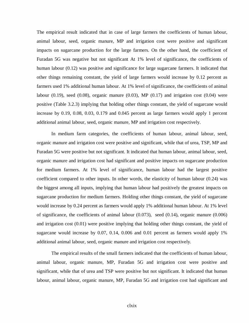
clxix
The empirical result indicated that in case of large farmers the coefficients of human labour,
animal labour, seed, organic manure, MP and irrigation cost were positive and significant
impacts on sugarcane production for the large farmers. On the other hand, the coefficient of
Furadan 5G was negative but not significant At 1% level of significance, the coefficients of
human labour (0.12) was positive and significance for large sugarcane farmers. It indicated that
other things remaining constant, the yield of large farmers would increase by 0.12 percent as
farmers used 1% additional human labour. At 1% level of significance, the coefficients of animal
labour (0.19), seed (0.08), organic manure (0.03), MP (0.17) and irrigation cost (0.04) were
positive (Table 3.2.3) implying that holding other things constant, the yield of sugarcane would
increase by 0.19, 0.08, 0.03, 0.179 and 0.045 percent as large farmers would apply 1 percent
additional animal labour, seed, organic manure, MP and irrigation cost respectively.
In medium farm categories, the coefficients of human labour, animal labour, seed,
organic manure and irrigation cost were positive and significant, while that of urea, TSP, MP and
Furadan 5G were positive but not significant. It indicated that human labour, animal labour, seed,
organic manure and irrigation cost had significant and positive impacts on sugarcane production
for medium farmers. At 1% level of significance, human labour had the largest positive
coefficient compared to other inputs. In other words, the elasticity of human labour (0.24) was
the biggest among all inputs, implying that human labour had positively the greatest impacts on
sugarcane production for medium farmers. Holding other things constant, the yield of sugarcane
would increase by 0.24 percent as farmers would apply 1% additional human labour. At 1% level
of significance, the coefficients of animal labour (0.073), seed (0.14), organic manure (0.006)
and irrigation cost (0.01) were positive implying that holding other things constant, the yield of
sugarcane would increase by 0.07, 0.14, 0.006 and 0.01 percent as farmers would apply 1%
additional animal labour, seed, organic manure and irrigation cost respectively.
The empirical results of the small farmers indicated that the coefficients of human labour,
animal labour, organic manure, MP, Furadan 5G and irrigation cost were positive and
significant, while that of urea and TSP were positive but not significant. It indicated that human
labour, animal labour, organic manure, MP, Furadan 5G and irrigation cost had significant and

clxx
positive impacts on sugarcane production for small farmers. At 1% level of significance human
labour had the largest and positive coefficients compared to other inputs.
Table 3.2.3 Maximum likelihood estimates for parameters of farm size-specific Cobb-Douglas stochastic frontier production and technical inefficiency model for sugarcane
Independent variables Parameters Farm Size Group
Large Medium Small
Constant β0 7.628(0.455) 6.991(0.495) 9.11(0.826)
Ln Human labour β1 0.118*(0.033) 0.235*(0.039) 0.452*(0.049)
Ln Animal labour β2 0.196*(0.055) 0.073**(0.039) 0.129*(0.049)
Ln Seed β3 0.081*(0.024) 0.143*(0.040) -0.124(0.121)
Ln Organic manure β4 0.034*(0.006) 0.006*(0.002) 0.008*(0.003)
Ln Urea β5 0.065(0.118) 0.113(0.089) 0.128(0.116)
Ln TSP β6 0.021(0.037) 0.064(0.044) 0.0017(0.069
Ln MP β7 0.169*(0.045) 0.037(0.027) 0.102*(0.048)
Ln Furadan 5G β8 -0.027(0.037) 0.011(0.010) 0.014*(0.010)
Ln Irrgation β9 0.035*(0.007) 0.014*(0.004) 0.007*(0.0037)
Technical inefficiency model:
Constant δ0 0.302(0.269) 0.471*(0.094) 0.469(0.379)
Experience δ1 -0.006**(0.003) -0.003*(0.001) -0.012*(0.002)
Age δ2 -0.006**(0.003) 0.0004(0.001) -0.001(0.002)
Education (year) δ3 0.010(0.010) -0.003(0.002) -0.016*(0.005)
Visit by field the worker δ4 -0.075**(0.035) -0.053*(0.009) -0.053*(0.026)
Farm size δ5 -0.130**(0.067) -0.110*(0.033) 0.046(045)
Dummy for sugarcane training (1=Yes, 0= otherwise) Dt
δ6 -0.092*(0.031) -0.035*(0.011) -0.067**(0.038)
Variance parameters :
Sigma- squared σ2 0.021*(0.005) 0.011*(0.001) 0.0067*(0.001)
Gamma γ 0.999*(0.0001) 0.999*(0.030) 0.999*(0.256)
Log likelihood function 66.415 151.756 82.878
* and ** indicate significant at 1% and 5% level of probability. Figures in the parentheses indicate standard error

clxxi
In other words, the elasticity of human labour (0.45) for small farmers was the biggest of all
other groups. Other things being constant the yield of sugarcane would increase by 0.45% as
farmers used 1% additional human labour in different types of management practices like, seed
cutting, land preparation, planting, weeding, mulching, application of fertilizers, tying, earthling
up, harvesting and carrying. At 1% level of significance, the coefficients of animal labour (0.13),
organic manure (0.008), MP (0.10), Furadan 5G (0.01) and irrigation cost (0.007) were positive
(Table 3.2.3) implying that holding other things constant, the yield of sugarcane would increase
by 0.139, 0.008, 0.10, 0.01 and 0.007 percent for small farmers would apply 1 percent additional
human labour, animal labour, organic manure, MP, Furadan 5G and irrigation cost respectively.
In the technical inefficiency model the coefficients of experience of large, medium and
small farmers were negative and significant. The negative and significant coefficient of
experience measured in years indicated that the farmers with more experience tend to be less
inefficient or more efficient. So, farming experience (the farmers who cultivate sugarcane for
longer period can increase the technical efficiency. This result is in line with those of Ahmad
(2002), Kamruzzaman et al. (2008), Coelli (1996), Bettese et al. (1992) and Hassan et al.
(2005). At 5% level of significance the negative coefficient of age of large farmers indicated that
the older farmers are more efficient than the younger ones. The negative and significant
coefficient of education of small farmers indicated that the farmers with greater years of formal
schooling tend to decrease inefficiency or increase technical efficiency. This indicates that the
farmers with more education respond more readily in using the new technology and produce
output closer to the frontier. This result is similar to that of Seyoum et al. (1998); Dey, et al.
2000; Pagan, (2001). The positive but non- significant coefficient of education of large farmers
indicated that the educated large farmers were less efficient than the less educated large farmers.
Usually, the high educated large farmers do not operated by themselves. They are engaged on
other services and business and they depend on others for sugarcane cultivation. On the other
hands, the less educated large farmers efficiently operate their lands by themselves. The
estimated coefficient of the farm size variable was negative and significant of large and medium
farmers, which indicated that the increase of sugarcane farm size tends to decrease inefficiency
or increase efficiency. This is similar to that of Rahman et al. (2000), Ahmed et al. (2002). The

clxxii
coefficient of visit by the field workers and sugarcane training were negative and significant of
three categories of farmers. This implied that the regular visit by field workers to the farmers’
sugarcane plot tends to decrease inefficiency or increase efficiency. This is similar to that of
Rahman et al. (2000), Chaudhry (2001), and Islam (2003). Training improves skills and the
result supports that professional training reduces inefficiency. The coefficient of sugarcane
training (Dt) was negative and significant. It indicated that the training on sugarcane production
reduced the production inefficiency and increased the technical efficiencies of sugarcane
production. If a farmer gets more training programmes, his level of inefficiencies would
decrease. The estimated values of variance parameters were large and significantly different
from zero which indicated a good fit and correctness of the specified distributional assumption.
The significant value of γ also indicated that there were significant technical inefficiency effects
in the production of sugarcane.
3.2.5 Technical Efficiency and its Distribution
The estimated location specific and farm size specific technical efficiencies are presented
in the Table 3.2.4. It was observed that the mean value of technical efficiency was 0.76 with a
range from 0.53 to 0.89. This implied that, on average, the sugarcane production in the study
areas were producing sugarcane to about 76 percent of the potential (stochastic) frontier
production level, given the levels of their inputs and the technology currently being used. This
also indicated that there existed an average level of technical inefficiency of 24 percent. The
technical efficiency of large, medium and small farmers was 84%, 77% and 68% respectively.
The variation in technical efficiency was observed higher with large farmers (ranged 60-89%)
than medium (ranged 60-88%) and small (ranged 53-79%) farmers. On the other hand, the mean
technical efficiency was higher at Rajshahi (80%) as compared to Thakurgaon (73%) and
Panchagar (76%). The variation of technical efficiency was higher at Thakurgaon ranged 54-
88% whereas, it was 60-89% at Panchagar and 63-88% at Rajshahi. The higher variation in
technical efficiency implied that technical efficiency was fluctuating to some extent for small
farmers as well as for the farmers at Thakurgaon in sugarcane production.

clxxiii
Considering different locations, the farmers at Rajshahi were found to be more
technically efficient in sugarcane production compared to the farmers of other locations. Seventy
nine percent of the farmers at Rajshahi achieved technical efficiency level of more
Table 3.2.4 Farm specific technical efficiency of sugarcane production
Location Farm category
No. of farms
Technical efficiency
Mean Maximum Minimum Standard deviation
Rajshahi Large 10 0.88 0.88 0.82 0.02
Medium 51 0.78 0.82 0.66 0.02
Small 39 0.74 0.79 0.63 0.01
All 100 0.80 0.88 0.63 0.02
Thakurgaon Large 14 0.79 0.86 0.60 0.04
Medium 62 0.79 0.88 0.73 0.04
Small 24 0.62 0.76 0.54 0.03
All 100 0.73 0.88 0.54 0.04
Panchagar Large 34 0.85 0.89 0.65 0.02
Medium 54 0.75 0.79 0.60 0.03
Small 12 0.70 0.78 0.65 0.04
All 100 0.76 0.89 0.60 0.04
All Large 58 0.84 0.89 0.60 0.03
Medium 167 0.77 0.88 0.60 0.04
Small 75 0.68 0.79 0.53 0.04
All 300 0.76 0.89 0.53 0.04
Source: Field survey (2007-08) than 70 percent (Table 3.2.5). On the other hand, 78 percent farmers at Thakurgaon and 62
percent of the farmers at Panchagar achieved technical efficiency level more than 70 percent. On

clxxiv
the contrary, more number of farmers at Panchagar (38%) achieved technical efficiency level of
less than 70% followed by Thakurgaon (22%) and Rajshahi (21%).When considering the farm
categories, it was observed that 79 percent large farmers obtained more than 70 percent technical
efficiency level. On the other hand, 80 percent of the medium and 51 percent of the small
farmers achieved more than 70 percent technical efficiency level (Figure 3.21). On the contrary,
49 percent of the small, 20 percent of the medium and 21 percent of
2122
38
59
43
36
20
35
26
0 0 00
10
20
30
40
50
60
Farm
ers
(%)
<70 71-80 81-90 91-100
Technical efficiency (%)
Rajshahi Thakurgaon Panchag
2119
49454646
34 34
5
0 0 00
5
10
15
20
25
30
35
40
45
50
Farm
ers
(%)
<70 71-80 81-90 91-100
Technical efficiency (%)
Large Medium Small
Figure 3.20 Technical efficiency level of sugarcane producers in different locations
Figure 3.21 Technical efficiency level of sugarcane producers by different farm categories

clxxv
Table 3.2.5 Frequency distribution of technical efficiency of sugarcane production
Region/ Location
Farm category
Number of farmer under different efficiency level (%) < 70 71-80 81-90 91-100 All
Rajshahi Large - - 10(100) - 10(100) Medium 1(2) 40(78) 10(20) - 51(100) Small 20(51) 19(49) - - 39(100) All 21(21) 59(59) 20(20) - 100(100) Thakurgaon Large 7(50) 7(50) - - 14(100) Medium - 31(50) 31(50) - 62(100) Small 15(62) 5(21) 4(17) 24(100) All 22(22) 43(43) 35(35) - 100(100) Panchagar Large 5(15) 19(57) 10(28) - 34(100) Medium 31(58) 7(12) 16(30) - 54(100) Small 2(17) 10(83) - - 12(100) All 38(38) 36(36) 26(26) - 100(100) All Large 12(21) 26(45) 20(34) - 58(100) Medium 32(19) 78(46) 57(34) - 167(100) Small 37(49) 34(46) 4(5) - 75(100) All 81(27) 138(46) 81(27) - 300(100) Figures in the parentheses indicate percent of total Source: Field survey (2007-08)
the large farmers achieved less than 70 percent technical efficiency level. Technical efficiency
level of different farm categories indicated that that there was no farmer above the level of 90
percent denoting that technical efficiency was somewhat satisfactory in sugarcane production
(Table 3.2.5).
3.2.6 Maximum Likelihood Estimates of Farm-specific Stochastic Frontier Cost Function and Economic Inefficiency Model
The economic efficiencies were estimated for all and different locations and different
farm – size groups with the help of derived normalized cost frontier by maximum livelihood
estimate (MLE) method using a computer software, Frontier 4.1 (Coelli, 1996). Asides from
estimates of coefficients the model, provides sigma squared (σ2 ), gama (γ) and log livelihood
function. To estimate economic efficiency indices for sugarcane production in the study areas,

clxxvi
the stochastic frontier cost function with production cost as dependent variable was estimated in
which all input prices were normalized by price of seed. The maximum likelihood Estimates
(MLE) of the coefficients of stochastic Cobb- Douglas cost performances are presented in Table
3.2.6.
The empirical results indicated that the coefficients of output, human labour price, MP
price and dummy for location (D2) were positive and significant implying that an increase in the
magnitudes of these variables would result in the corresponding increase of cost of producing
sugarcane for the farmers. The coefficients of animal labour price, organic manure price,
Furadan 5G price, irrigation cost, and dummy of location (D1) were positive but not significant.
They had positive effect on production cost but not significant. At 1% level of significance the
coefficients of output (0.80) was positive implying that holding other things constant, 1 percent
increase in output will lead the production cost to increase by 0.80 percent. At 1% level of
dummy variable (D2), Rajshahi was positive and significant which implies that the production
cost of sugarcane at Rajshahi was higher than that of other locations. At 5% level of
significance, the coefficient of human labour price (0.07) and of MP price (1.32) were positive,
which implies that holdings other things constant the production cost would increase by 0.07
and 1.32 percent as 1% additional increase in human labour cost and MP cost. On the other hand
the coefficients of urea price and TSP price were negative but not significant
Table 3.2.6 Maximum likelihood estimates for parameters of Cobb-Douglas stochastic normalized cost frontier and economic inefficiency model for sugarcane
Independent variables Parameters Coefficients Standard
error t-ratio
Constant β0 -0.773 0.463 -1.667
Ln Output (Tk/ha) β1 0.801* 0.033 23.637
Ln Human labour (Tk /man days) β2 0.068** 0.038 1.796
Ln Animal labour (Tk/pair-days) β3 0.004 0.028 0.144
Ln Organic manure (Tk/kg) β4 0.051 0.043 1.175
Ln Urea (Tk/kg) β5 -0.041 0.039 -1.047
Ln TSP (Tk/kg) β6 -0.454 0.609 -0.745
Ln MP (Tk/kg) β7 1.323** 0.600 2.204

clxxvii
Ln Furadan 5G (Tk/kg) β8 0.003 0.003 0.832
Ln Irrgation (Tk/ha) β9 0.0003 0.002 0.156
Dummy for location (Thakurgaon=1, others=0) D1
β10 0.029 0.017 1.67
Dummy for location (Rajshahi=1, others=0) D2
β11 0.101* 0.014 7.015
Technical inefficiency model:
Constant δ0 0.017 0.090 0.141
Experience (years) δ1 -0.002** 0.001 -1.204
Age (years) δ2 0.0008 0.0016 0.489
Education (year of schooling) δ3 -0.007** 0.003 -2.330
Visit by field worker (no.) δ4 -0.026* 0.009 -2.88
Farm size (ha) δ5 -0.018 0.024 -0.754
Dummy for sugarcane training (1=Yes, 0= otherwise) Dt
δ6 -0.089* 0.030 -2.96
Variance parameters :
Sigma- squared σ2 0.005* 0.0005 10.392
Gamma γ 0.016 0.005 0.170
Log likelihood function 364.09
* and ** indicate significant at 1% and 5% level of probability. Dependent variable = Production cost (Tk/ha)
In inefficiency model, the coefficient of experience was negative and significant at 5%
level. This indicated that the farmers, who had greater experience about sugarcane production,
are economically more efficient than the less experienced. Better performance among the
experienced farmers is attributable to significantly lower labour use for per unit of sugarcane
production, lower wage rate, lower input price, followed the agronomical practices (plantation,
weeding, fertilizer application, insects and diseases control, irrigation, tying, etc) in proper way
and proper time than the less experienced farmers. The coefficient of farmers’ education was
negative and significant. This indicates that the farmers with more education become more
efficient. The coefficient for the visit by the field worker was negative and significant. This
implied that the regular visit by field workers to the farmers’ sugarcane plot tends to decrease the
economic inefficiency or increase efficiency. Dummy for sugarcane training were negative and
significant which indicated that the sugarcane training decrease the economic inefficiency. The

clxxviii
estimated value of the variance parameter σ2 was large and significantly different from zero,
which indicated a good fit and correctness of the specified distributional assumption.
3.2.7 Maximum Likelihood Estimates of Location-specific Stochastic Frontier Cost Function and Economic Inefficiency Model
The maximum likelihood estimates of the coefficients of location specific stochastic
frontier cost function and inefficiency effect are presented in table 3.2.7. The empirical results
indicated that at Rajshahi, the coefficients of output (0.92), human labour (0.24) and irrigation
cost (0.004) were positive and significant implying that an increase in the magnitudes of these
variables would result in corresponding increase of cost of producing sugarcane. The coefficient
of organic manure cost was negative and significant 1% level which meant that an increase in the
magnitudes of organic manure cost would result in the corresponding decrease of cost of
producing sugarcane. The coefficients of urea, MP, Furadan 5G price were also positive but not
significant which implies that urea, MP, Furadan 5G price had positive impact on production
cost but not significant. On the other hand the coefficients of animal labour and TSP price were
negative but not significant.
At Thakurgaon the coefficients of output (0.74), organic manure price (0.29), MP pricet
(0.06) and Furadan 5G price were positive and significant implying that an increase in the
magnitude of these variables would result in the corresponding increase of cost of producing
sugarcane for the farmers. The coefficient of human labour price (0.11) was positive but not
significant. On the other hand the coefficients of animal labour price (0.007), urea price (0.19),
TSP price (0.34) and irrigation costs (0.001) were negative but not significant implying that the
coefficients of animal labour price, urea price, TSP price and irrigation cost had decreased
sugarcane production cost but this was not significant.
At Panchagar, the coefficients of output, human labour price, MP price and irrigation cost
were positive and significant implying that an increase in the magnitude of these variables would
result in the corresponding increase of cost of producing sugarcane for the farmers. The
coefficients of animal labour, organic manure and Furadan 5G price were found to be positive
but not significant. On the other hand the coefficient of irrigation cost was negative and
clxxix
significant which implies that an increase in the magnitude of this variable would result in the
decrease of sugarcane production cost for the farmers. The coefficients of urea and TSP cost
were found to be negative but not significant.
In the inefficiency model the coefficients of experience of Rajshahi and Panchagar was negative
and significant. This indicates that the economic inefficiency of the sugarcane farmer of Rajshahi
and Panchagar decrease with the increase of the experiences of the farm operator. The
experienced farmers are more efficient than less experienced ones in economic efficiency by
using lower input cost. The coefficient of education was negative and significant at 5% percent
level, which implied that the sugarcane farmers of Panchagar with greater year of schooling tend
to be less economic inefficient. The coefficient of visit by the field workers of Rajshahi and
Thakurgaon was negative and significant. This implied that the regular visit by field workers to
the farmers’ sugarcane plot tends to decrease the economic inefficiency or increase efficiency.
The coefficient of sugarcane training (Dt) was negative and significant. It indicated that the
training on sugarcane production reduced the economic inefficiency and increased the technical
efficiencies of sugarcane production. If a farmer gets more training programmes, his level of
inefficiencies would decrease. The estimated values of variance parameters were large and
significantly different from zero which indicated a good fit and correctness of the specified
distributional assumption. The significant value of γ also indicated that there were significant
technical inefficiency effects in the production of sugarcane.

clxxx
Table 3.2.7 Maximum likelihood estimates for parameters of location–specific Cobb-Douglas stochastic normalized cost frontier and economic inefficiency effect model
Independent variables Param-eters
Locations
Rajshahi Thakurgaon Panchagar
Constant β0 -1.609**(0.812) -0.046(1.059) -0.656(1.005)
Ln output (Tk/ha) β1 0.922*(0.058) 0.739*(0.067) 0.726*(0.052)
Ln Human labour (Tk /man days)
β2 0.239**(0.118) 0.110(0.111) 0.120*(0.038)
Ln Animal labour (Tk/pair-days)
β3 -0.019(0.041) -0.007(0.053) 0.007(0.025)
Ln Organic manure (Tk/kg) β4 -0.123*(0.049) 0.286*(0.088) 0.209(0.213)
Ln Urea (Tk/kg) β5 0.015(0.049) -0.195(0.105) -0.012(0.029)
Ln TSP (Tk/kg) β6 -0690(0.417) -0.338(0.577) -0.592(0.710)
Ln MP (Tk/kg) β7 1.137(0.734) 1.163**(0.589) 1.566**(0.702)
Ln Furadan 5G (Tk/kg) β8 0.003(0.003) 0.060**(0.394) 0.009(0.017)
Ln Irrgation (Tk/ha) β9 0.004**(0.002) -0.0014(.009) -0.006**(0.003)
Inefficiency effect model:
Constant δ0 0.246*(0.076) 0.033(0.513) 0.094(0.079)
Experience (years) δ1 0.002(0.002) 0.0003(0.001) -0.004**(0.002)
Age (years) δ2 -0.004*(0.001) 0.0005(0.0009) 0.0002(0.0014)
Education (year of schooling)
δ3 -0.006(0.004) 0.002(.003) -0.012*(0.004)
Visit by field worker (no.) δ4 -0.016(0.013) -0.024**(0.013) 0.014(0.012)
Farm size (ha) δ5 0.035(0.023) -0.032(0.14) 0.016(0.016)
Dummy for sugarcane training (1=Yes, 0= otherwise) Dt
δ6 -0.037(0.036) -0.009(0.021) -0.043(0.030)
Variance parameters :
Sigma- squared σ2 0.004*(0.0007) 0.006*(0.001) 0.003*(0.0008)
Gamma γ 0.086(0.199) 0.005(3.002) 0.039(0.226)
Log likelihood function 145.383 107.726 154.790
* and ** indicate significant at 1% and 5% level of probability. Figures in the parentheses indicate standard error Dependent variable = Production cost (Tk/ha)

clxxxi
3.2.8 Maximum Likelihood Estimates of Farm-size Specific Stochastic Frontier Cost Function and Economic Inefficiency Model
The empirical results from farm specific estimates showed that for the large farms, the
coefficients of human labour and MP prices were positive and significant implying that an
increase in the magnitudes of these variables would result in the corresponding increase of cost
of producing sugarcane (Table 3.2.8). The coefficients of output, organic manure price and
dummy location for Thakurgaon (D1) were found to be positive but not significant. On the other
hand, the coefficients of animal labour, urea, TSP, Furadan 5G price, irrigation costs and dummy
location for Rajshahi (D2) were negative but not significant implying that an increase in the use
of animal labour, urea, TSP, Furadan 5G and irrigation costs would result in the decrease of cost
of producing sugarcane for the large farmers but not significantly. In case of medium farmers the
coefficient of output (0.78), organic manure price (0.14), MP price (1.26), D1 and D2 were
positive and significant (Table 3.2.8) implying that an increase in the magnitude of these
variables would result in the corresponding increase of cost of producing sugarcane for the
farmers. The coefficients of human labour, animal labour, Furadan 5G cost and irrigation cost
were positive but not significant.
On the other hand, the coefficients of urea and TSP price were found to be negative but also not
significant, which implied that an increase in the magnitude of these variables would result in
the corresponding decrease of cost of producing sugarcane for the farmers but not significant. In
case of small farmers the coefficient of output and human labour price were positive and
significant which implied that an increase in the magnitude of these variables would result in the
corresponding increase of economic efficiency. On the other hand the coefficient of organic
manure price was negative and significant which implied that an increase in the magnitudes of
this variable would result in the decrease of cost of producing sugarcane for the small farmers.
In inefficiency effects model the coefficients of experience of large and small farmers
were negative and significant which indicated that the experience of the farmers decreases

clxxxii
economic inefficiencies and increases economic efficiencies. The coefficient of large farmers’
education was negative and significant, which indicates that the education of large farmers
decreases economic inefficiency and increases efficiency. For medium farmers the
Table 3.2.8 Maximum likelihood estimates for parameters of farm size –specific Cobb-Douglas stochastic normalized cost frontier and economic inefficiency effect model
Independent variables Param-eters
Farm categories
Large Medium Small
Constant β0 1.109(1.252) -0.752(0.634) -0.841(0.975)
Ln Output (Tk/ha) β1 0.065(1.252) 0.784*(0.048) 0.882*(0.091)
Ln Human labour (Tk /man days) β2 0.134**(0.073) 0.049(0.051) 0.266*(0.124)
Ln Animal labour (Tk/pair-days) β3 -0.007(0.037) 0.008(0.036) -0.042(0.085)
Ln Organic manure (Tk/kg) β4 0.277(0.205) 0.138*(0.057) -0.551*(0.269)
Ln Urea (Tk/kg) β5 -0.040(0.075) -0.070(0.055) 0.097(0.222)
Ln TSP (Tk/kg) β6 -0.925(0.756) -0.309(0.429) -0.821(0.860)
Ln MP (Tk/kg) β7 1.629*(0.648) 1.262*(0.428) 1.236(0.837)
Ln Furadan 5G (Tk/kg) β8 -0.020(0.027) 0.004(0.005) 0.006(0.007)
Ln Irrgation (Tk/ha) β9 -0.009(0.007) 0.0003(0.003) 0.004(0.004)
Dummy for location (Thakurgaon=1, others=0) D1
β10 0.062(0.035) 0.095*(0.023) 0.058(0.047)
Dummy for location (Rajshahi=1, others=0) D2
β11 -0.098(0.216) 0.046**(0.023) -0.019(0.165)
Inefficiency effect model:
Constant δ0 0.326(0.251) 0.111*(0.043) -0.017(0.124)
Experience (years) δ1 -0.050*(0.004) -0.0008(0.0009) -0.006*(0.002)
Age (years) δ2 -0.007(0.005) 0.000(0.0008) 0.003(0.002)
Education (year of schooling) δ3 -0.035*(0.011) -0.002(0.002) -0.006(0.007)
Visit by field worker (no.) δ4 -0.034**(0.018) --0.004(0.006) -0.040*(0.015)
Farm size (ha) δ5 -0.053(0.045) -0.075*(0.20) -0.002(0.023)
Dummy for sugarcane training (1=Yes, 0= otherwise) Dt
δ6 -0.026*(0.006) -0.0003(0.017) -0.010(0.033)

clxxxiii
Variance parameters :
Sigma- squared σ2 0.004*(0.001) 0.005*(0.0005) 0.005*(0.0005)
Gamma γ 0.345(0.243) 0.001(0.009) 0.047*(0.014)
Log likelihood function 68.819 215.400 99.777 * and ** indicate significant at 1% and 5% level of probability. Figures in the parentheses indicate standard error Dependent variable= Production cost (Tk/ha).
farm size had negative and significant effect on economic inefficiency. This implied that the
large farms are relatively more economically efficient than the smaller ones.
The large size farmers operate large size of sugarcane area, as a result per unit production
cost decreases and ultimately increased the economic efficiency. Better performance among
larger farms is attributable to significantly lower labour use per unit of output produced on large
farms than an smaller ones (Sharma et al., 1997). The coefficients of visit by field worker of
large and small farmers were negative and significant. This implied that the regular visit by field
workers to the farmers’ sugarcane plot tends to decrease the economic inefficiency or increase
efficiency. The coefficient of sugarcane training (Dt) of large farmers was negative and
significant. It indicated that the training on sugarcane production of large farmers reduced the
economic inefficiency and increased the technical efficiencies of sugarcane production. It also
indicated that the large farmers received the training on sugarcane production and applies it
properly. The estimated values of variance parameters were large and significantly different from
zero which indicated a good fit and correctness of the specified distributional assumption. The
significant value of γ also indicated that there were significant technical inefficiency effects in
the production of sugarcane.
3.2.9 Economic Efficiency and its Distribution
Locations specific and farm size specific economic efficiency was estimated by using
cost function and normalized by seed price (Table 3.2.9). It was observed that the mean value of
economic efficiency was 0.62 with a range from 0.30 to 0.78. This implied that, on average, the

clxxxiv
sugarcane producers in the study area were producing sugarcane to about 62 percent of the
potential (stochastic) frontier levels, given the levels of their inputs and the technology currently
being used. This also indicated that there existed an average level of economic inefficiency of 38
percent. Considering the farm categories, the mean economic efficiencies of large, medium and
small farms were 63%, 61% and 62% respectively. The variation in economic efficiency was
observed higher with the medium (ranged from 30-78%) and small (ranged from 30-73%)
farmers than the large (ranged from 40-74%) farmers. It was found that 69 percent of the large
farmers obtained economic efficiency level of more than 60 percent in comparison to small
farmers (67) and medium (61) percent, indicating better performance was observed in the large
farmers (Table 3.2.10 and Figure 3.23). On the contrary, 6 percent of the medium farmers and 4
percent of the small and 3 percent of the large farmers achieved economic efficiency level of less
than 50 percent which indicated that large farmers are more economically efficient than small
and medium farmers. It also indicated that economic efficiency was somewhat unstable for small
and medium farmers due probably to their poorest resources base and resources constraints.
Table 3.2.9 Farm specific economic efficiency of sugarcane production
Location Farm category
No. of farms
Economic efficiency
Mean Maximum Minimum Standard deviation
Rajshahi Large 10 0.69 0.69 0.59 0.02 Medium 51 0.51 0.74 0.46 0.06 Small 39 0.60 0.73 0.30 0.08 All 100 0.63 0.74 0.30 0.06 Thakurgaon Large 14 0.58 0.70 0.40 0.08 Medium 62 0.59 0.71 0.30 0.08 Small 24 0.62 0.70 0.41 0.06 All 100 0.60 0.71 0.30 0.08 Panchagar Large 34 0.64 0.74 0.46 0.06 Medium 54 0.63 0.78 0.30 0.07 Small 12 0.63 0.71 0.54 0.05 All 100 0.63 0.78 0.30 0.07 All Large 59 0.63 0.74 0.40 0.07

clxxxv
Medium 167 0.61 0.78 0.30 0.07 Small 75 0.62 0.73 0.30 0.07 All 300 0.62 0.78 0.30 0.07
Source: Field survey (2007-08)
49
2
27
38
28
5151
62
18
2
8
00 00
10
20
30
40
50
60
70
Farm
ers
(%)
<50 50-60 61-70 71-80 81-100
Economic efficiency (%)
Rajshahi Thakurgaon Panchagar
36 4
28
3329
43
56
62
26
5 50 0 0
0
10
20
30
40
50
60
70
Farm
ers
(%)
<50 50-60 61-70 71-80 81-100
Economic efficiency (%)
Large Medium Small
Figure 3.22 Economic efficiency level of
sugarcane producers in different locations
Figure 3.23 Economic efficiency level of sugarcane producers by different farm categories
Table 3.2.10 Frequency distribution of economic efficiency of sugarcane farmers Region/ Location
Farm category
Number of farmer under different efficiency level (%)
≤ 50 51-60 61-70 71-80 80-100 All
Rajshahi Large - - - 10(100) - 10(100)
Medium 2(4) 16(31) 28(55) 5(10) - 51(100)
Small 2(5) 11(29) 23(59) 3(7) - 39(100)
All 4(4) 27(27) 51(51) 18(18) - 100(100)
Thakurgaon Large 1(7) 8(58) 5(35) - - 14(100)
Medium 7(11) 23(37) 30(49) 2(3) - 62(100)
Small 1(4) 7(29) 16(67) - - 24(100)
All 9(9) 38(38) 51(51) 2(2) - 100(100)
Panchagar Large 1(3) 8(23) 20(59) 5(15) - 34(100)
Medium 1(2) 16(30) 35(64) 2(4) - 54(100)
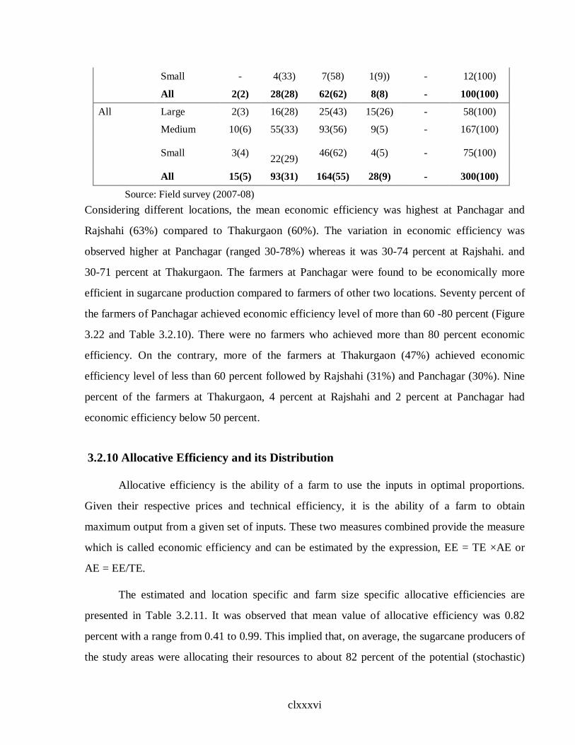
clxxxvi
Small - 4(33) 7(58) 1(9)) - 12(100)
All 2(2) 28(28) 62(62) 8(8) - 100(100)
All Large 2(3) 16(28) 25(43) 15(26) - 58(100)
Medium 10(6) 55(33) 93(56) 9(5) - 167(100)
Small 3(4) 22(29) 46(62) 4(5) - 75(100)
All 15(5) 93(31) 164(55) 28(9) - 300(100)
Source: Field survey (2007-08) Considering different locations, the mean economic efficiency was highest at Panchagar and
Rajshahi (63%) compared to Thakurgaon (60%). The variation in economic efficiency was
observed higher at Panchagar (ranged 30-78%) whereas it was 30-74 percent at Rajshahi. and
30-71 percent at Thakurgaon. The farmers at Panchagar were found to be economically more
efficient in sugarcane production compared to farmers of other two locations. Seventy percent of
the farmers of Panchagar achieved economic efficiency level of more than 60 -80 percent (Figure
3.22 and Table 3.2.10). There were no farmers who achieved more than 80 percent economic
efficiency. On the contrary, more of the farmers at Thakurgaon (47%) achieved economic
efficiency level of less than 60 percent followed by Rajshahi (31%) and Panchagar (30%). Nine
percent of the farmers at Thakurgaon, 4 percent at Rajshahi and 2 percent at Panchagar had
economic efficiency below 50 percent.
3.2.10 Allocative Efficiency and its Distribution
Allocative efficiency is the ability of a farm to use the inputs in optimal proportions.
Given their respective prices and technical efficiency, it is the ability of a farm to obtain
maximum output from a given set of inputs. These two measures combined provide the measure
which is called economic efficiency and can be estimated by the expression, EE = TE ×AE or
AE = EE/TE.
The estimated and location specific and farm size specific allocative efficiencies are
presented in Table 3.2.11. It was observed that mean value of allocative efficiency was 0.82
percent with a range from 0.41 to 0.99. This implied that, on average, the sugarcane producers of
the study areas were allocating their resources to about 82 percent of the potential (stochastic)

clxxxvii
frontier levels for sugarcane production. This also indicated that there existed an average level of
allocative inefficiency of 18 percent. Considering the different locations, the highest variation
were obtained of the farmers (Table 3.2.11) at Thkurgaon (ranged from 41- 92%) followed by
Panchagar (ranged from 50- 99%) and Rajshahi (ranged from 48- 92%). The farmers at
Panchagar were found to be more allocatively efficient in sugarcane production compared to
other two locations. Fifty four percent of the farmers at Panchagar achieved allocative efficiency
level of more than 90 percent (Figure 3.24 and Table 3.2.12). On the other hand, 48 percent of
farmers at Thakurgaon and 33 percent of the farmers at Rajshahi achieved allocative efficiency
level more than 90 percent. On the contrary, more number of farmers at Rajshahi (22%) achieved
allocative efficiency level less than 80 percent followed by Thakurgaon (18%) and Panchagar
(3%). Forty three percent of the farmers at Rajshahi and Panchagar achieved within 81-90
percent allocative efficiency level followed by Thakurgaon 34 %. When consideration of
different farm categories were taken, it was observed that 87 percent of the larger farmers
obtained allocative efficiency level more than 80 percent in comparison with medium and small
farmers 86 and 81 percent respectively (Table 3.2.12 and Figure 3.25) indicating better
performance of large farmers.
Table 3.2.11 Farm specific allocative efficiency of sugarcane production
Location Farm category
No. of farms
Allocative efficiency
Mean Maximum Minimum Standard deviation
Rajshahi Large 10 0.78 0.78 0.71 0.04-
Medium 51 0.78 0.90 0.70 0.08
Small 39 0.81 0.92 0.48 0.11
All 100 0.79 0.92 0.48 0.08
Thakurgaon Large 14 0.73 0.81 0.67 0.10
Medium 62 0.75 0.81 0.41 0.11
Small 24 0.99 0.92 0.76 0.07
All 100 0.82 0.92 0.41 0.10
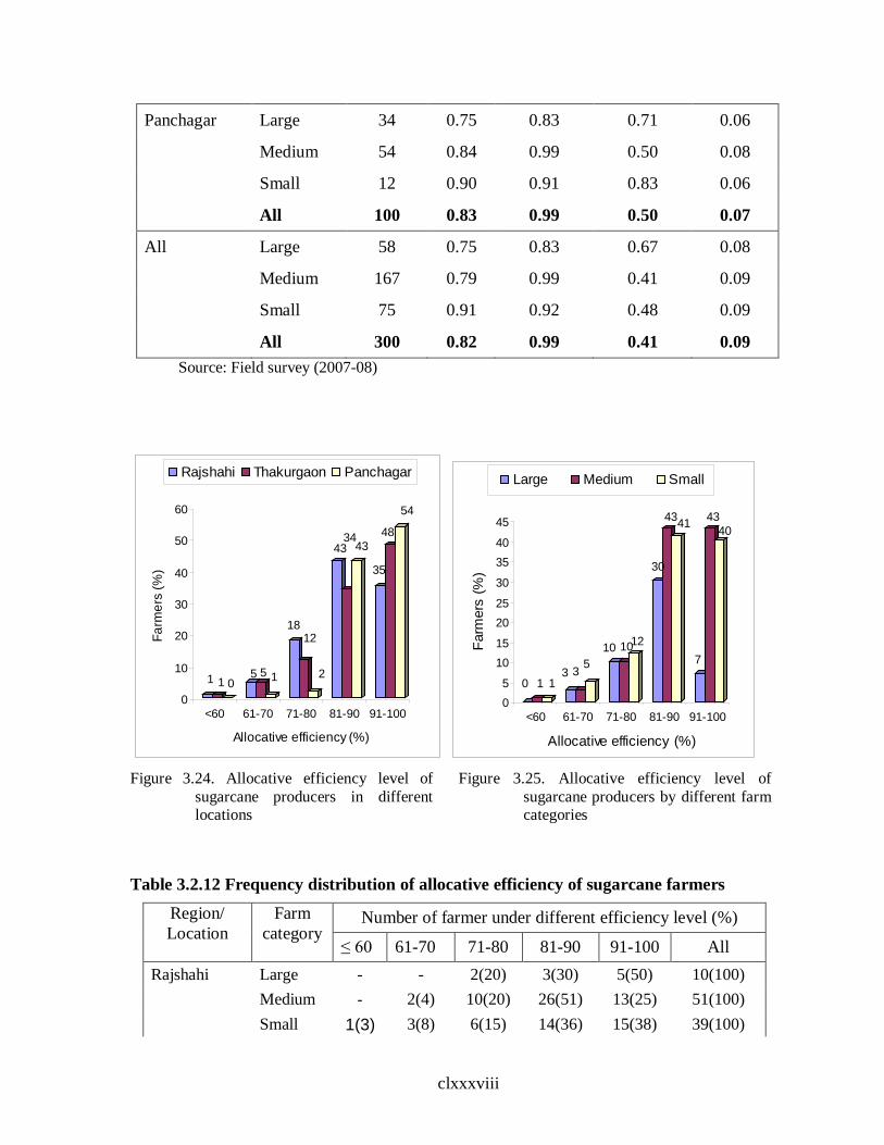
clxxxviii
Panchagar Large 34 0.75 0.83 0.71 0.06
Medium 54 0.84 0.99 0.50 0.08
Small 12 0.90 0.91 0.83 0.06
All 100 0.83 0.99 0.50 0.07
All Large 58 0.75 0.83 0.67 0.08
Medium 167 0.79 0.99 0.41 0.09
Small 75 0.91 0.92 0.48 0.09
All 300 0.82 0.99 0.41 0.09 Source: Field survey (2007-08)
1 1 05 5 1
1812
2
4334
43
35
48
54
0
10
20
30
40
50
60
Farm
ers
(%)
<60 61-70 71-80 81-90 91-100
Allocative efficiency (%)
Rajshahi Thakurgaon Panchagar
0 1 13 3 5
10 1012
30
4341
7
4340
05
1015
2025
30
3540
45
Farm
ers
(%)
<60 61-70 71-80 81-90 91-100
Allocative efficiency (%)
Large Medium Small
Figure 3.24. Allocative efficiency level of
sugarcane producers in different locations
Figure 3.25. Allocative efficiency level of sugarcane producers by different farm categories
Table 3.2.12 Frequency distribution of allocative efficiency of sugarcane farmers
Region/ Location
Farm category
Number of farmer under different efficiency level (%)
≤ 60 61-70 71-80 81-90 91-100 All Rajshahi Large - - 2(20) 3(30) 5(50) 10(100) Medium - 2(4) 10(20) 26(51) 13(25) 51(100) Small 1(3) 3(8) 6(15) 14(36) 15(38) 39(100)

clxxxix
All 1(1) 5(5) 18(18) 43(43) 35(35) 100(100) Thakurgaon Large - 1(7) 3(21) 5(36) 5(36) 14(100) Medium 1(2) 3(5) 7(11) 19(31) 32(51) 62(100) Small - 1(4) 2(8) 10(42) 11(46) 24(100) All 1(1) 5(5) 12(12) 34(34) 48(48) 100(100) Panchagar Large - 1(3) 1(3) 9(26) 23(68) 34(100) Medium - - - 27(50) 27(50) 54(100) Small - - 1(8) 7(59) 4(33) 12(100) All - 1(1) 2(2) 43(43) 54(54) 100(100) All Large - 2(3) 6(10) 17(30) 33(7) 58(100) Medium 1(1) 5(3) 17(10) 72(43) 72(43) 167(100) Small 1(1) 4(5) 9(12) 31(41) 30(40) 75(100) All 2(1) 11(4) 32(11) 120(40) 135(43) 300(100) Source: Field survey (2007-08)
3.3 YIELD GAP AND CONSTRAINTS IN SUGARCANE PRODUCTION
3.3.1 Introduction
Farm level yield of sugarcane is much lower than the yield obtained in on-station
experiment and farmers’ field demonstration. This difference is called the yield gap and it
resulted due to the variation in input use and poor management at farm level. Besides these, there
are many causes of constrains for yield gap. This chapter is devoted to the presentation and
discussion of yield gap and constraints in sugarcane production in Bangladesh. The specific
objectives of estimating the magnitude of yield gaps, sources contributing to the yield gaps, the
constraints responsible for yield gaps and to suggest appropriate measures to bridge the yield
gaps in sugarcane production in Bangladesh. The concept of yield gap came from the constraints
studies carried out by the International Rice Research Institute (IRRI) which makes a
quantitative difference between experiment station yield and the actual; farm yield. In this
chapter yield level of sugarcane in different situation is identified and then yield level is
quantified in relation to technical inefficiency.
cxc
3.3.2 Yield Gap
To estimate the yield gap in sugarcane production it is required to determine the yield
levels at different phases. According to IRRI methodology, the total yield gap (TYG) is the
difference between the potential yields (Yp – Experiment station yield) and the actual yield (Ya –
yield of sample farmers’ fields). The total yield gap (TYG) comprised Yield Gap-I (difference
between the potential yield and the potential farm yield (Yd –yield released on the demonstration
plots) and Yield Gap-II [difference between the potential farm yield (demonstration plot yield)
and the actual yield].
Experiment station Yield (Potential yield): It is the highest level of yield obtained by the
researchers in the experiment station under favorable environment and proper management
practices. BSRI (Bangladesh Sugarcane Research Institute) released varieties which presently
covers 95 percent of the total sugarcane area, experimental yield was estimated at 107.50 t/ha
(Rahman, et al. 2008,) (Figure 3.26).
Potential farm yield: Before releasing any variety to the farmers for adoption, it is sufficiently
tested under different agro-climatic conditions at research stations through trials and
demonstrations. It may not be always possible for the farmers to raise the crop productivity on
their farms to the level of research station. However, it would be realistic to aim at demonstration
plot yield (potential farm yield) level and achieved by on-trials. The potential farm yield was
considered 84.22 t/ha (BSRI, 2007-08).
Actual farm yield: Actual farm yield is the observed yield of any variety in the field. When a
variety of a crop is cultivated under farmers’ condition i.e. in farmers’ environment and
management with available technology and in the presence of constraints and stresses the yield
obtained is the actual farm yield. The observed yield of sugarcane varied with locations and farm
categories with a mean yield of 58.53 tonne /ha.

cxci
With the advent of new technology in agriculture, significant improvement in the crop
productivity was noticed. However, proper resource mix and appropriate cultural practices
become a pre-requisite for the adoption and success of new farm technology, which are often
beyond the reach of a majority of the farmers. It could be observed from Table 3.3.1 that there
existed a wide gap in the sugarcane productivity between the research station, the potential farm
(demonstration plots) and the sample farmers’ field.
115.94
84.22
58.53
0
20
40
60
80
100
120
Yiel
d (t/
ha)
Experimental yield Potential farm yield Actual farm yield
Figure 3.26 Experimental, potential and actual yield of sugarcane in Bangladesh
Table 3.3.1 Sugarcane yield realized and the estimated yield gap under different field situations
Sl. No. Particulars Yield (t/ha) 1. Experiment station (Potential) Yield 107.50
2. Potential farm yield 84.22
3. Actual farm yield
(a) Large farms 59.83
(b) Medium farms 59.09
(c) Small farms 56.67
(d) Overall farms 58.53
4. Yield Gap- I 23.28
5. Yield Gap- II

cxcii
(a) Large farms 24.39
(b) Medium farms 25.13
(c) Small farms 27.55
(d) Overall farms 25.69
6. Total yield gap
(a) Large farms 47.67
(b) Medium farms 48.41
(c) Small farms 50. 83
(d) Overall farms 48.97
Sources: BARC 2008, BSRI 2007-08 and survey 2007-08.
The magnitude of total yield gap worked out to be 48.97 t/ha, which comprised relatively higher
size of Yield Gap- II (25.69 t/ha) than Yield Gap- I (23.28) in the overall study area. Yield Gap-
I is calculated to understand to what extent the potential yield of research station possible is
achieved at the field demonstration. Similarly, the Yield Gap- II, between demonstration and
actual yield realized by the farmers, helps to know to what extent the farmers by all categories,
on an average, could have achieved at their field conditions. Yield Gap- I implied that greater
amount of potential yield was left untapped on the demonstration plots. This was attributable to
the significant environment differences and parity to the non-transferable component of
technology like cultural practices. Hence, the technology developed at research station could not
fully replicate on the demonstration plots. Farm size-group wise analysis of the total yield gap
over the districts showed the highest (50.83 t/ha) magnitude recoded on the small farms while the
lowest (46.67 t/ha) magnitude was noticed on the large farms.
The estimated index of yield gap worked out to be 45.55 percent (Table 3.3.2). So, there
existed a tremendous scope to improve the sugarcane production in the study area. The index of
potential yield worked out to be 54.44 percent in the overall category of sample farms. It may not
always be possible for the farmers to adopt certain aspects of new technology developed in
research stations due to differences in the environmental factors and other constraints operating
at the farm level. The sample farmers realized 69.50 percent (index of realized potential farm
yield) of the farm potential in the study area (Table 3.3.2). Thus, if all the recommended
packages and production technology used on the demonstration plots are adopted, the sample

cxciii
farmers could obtain 35 percent more sugarcane output. Farm size-group analysis showed that
the large cultivators obtained relatively better yield levels than their small counterparts.
Sugarcane being more capital intensive, it requires more of costly inputs. Due to better economic
conditions, large farmers probably made timely application of fertilizers and insecticides and
realized higher level of yield.
Table 3.3.2 Estimated indices of yield gaps in sugarcane under different field situation
Sl no. Particulars (%) 1. Index of yield gap:
(a) Large farms 44.34
(b) Medium farms 45.03
(c) Small farms 47.28
(d) Overall 45.55
2. Index of realized potential yield:
(a) Large farms 55.65
(b) Medium farms 54.96
(c) Small farms 52.72
(d) Overall 54.44
3. Index of realized potential farm yield:
(a) Large farms 71.04
(b) Medium farms 70.16
(c) Small farms 67.29
(d) Overall 69.50
Sources: BSRI, 2006-07; BARC, 2008 and field survey, 2007-08. 3.3.3 Yield Gap Due to Technical Inefficiency
The yield gap that occurred due to technical inefficiency was 24 percent (Table 3.2.4)
which caused 25.69 t/ha yield gap (difference between potential farm yield and actual farm
yield) of sugarcane (Table 3.3.3). Within the three locations the highest yield gap of sugarcane
due to technical inefficiency was recorded with the farmers at Thakurgaon (27.46 t/ha) followed
by Panchagar (26.60 t/ha) and Rajshahi (22.70 t/ha) implying that the farmers of Thakurgaon had
more potentiality to increase yield than the Rajshahi farmers of with their existing technology.
Considering the farm categories the highest yield gap was noted in small farmers (27.19 t/ha)

cxciv
followed by medium (25.11 t/ha) and large farmers (24.77 t/ha). It existed because of technical
and socio economic constraints.
Table 3.3.3 Yield gap of sugarcane due to technical inefficiency
Location/farm categories
No. of farms
Mean technical inefficiency (%)
Observed yield
(tonne/ha)
Potential yield
(tonne/ha)
Yield gap (tonne/ha)
Locations: Rajshahi 100 0.20 62.30 85.00 22.70
Panchagar 100 0.24 57.80 84.40 26.60
Thakurgaon 100 0.27 55.80 83.26 27.46
Farm categories:
Large 49 0.16 59.83 84.60 24.77
Medium 176 0.23 59.09 84.20 25.11
Small 75 0.32 56.67 83.86 27.19
All farms 300 0.24 58.53 84.22 25.69 Sources: Field survey 2007-08, BSRI, Table: 3.1.6, 3.1.7, 3.2.4
3.3.4 Yield Constraints
Yield gap is a great problem in agricultural sector. There are many constraints which pervert to
attain the potential level of yield of sugarcane in Bangladesh. Many of the farmers still follow
the traditional practice and they do not follow the modern technology. According to the opinions
given by the sugarcane growers the constraints of sugarcane farmers are divided into two groups
– technical and socio- economic constraints.
3.3.4.1 Technical Constraints:
Technical constraints are related to production techniques and technologies. The farmers in the
study areas mentioned a number of technical constraint which affected sugarcane production.
The summary of the sugarcane production constraints (Table 3.3.4) are discussed below:
cxcv
Lack of clean/ certified seed: Seed/ is a main factor of any production system. Although all the
farmers were found to produce high yielding varieties of sugarcane, 98 percent of them
mentioned that they had lacking of clean seed/good quality of seed and this constraint ranked 1st
among the constraints. Farmers are usually used sugarcane seed from their own plots or from
neighbors, which were not good quality seeds for their poor germination and were not free from
diseases. A few numbers of farmers used certified seed from sugar mills, these are not sufficient.
Irrespective of locations 94, 98 and 99 percent of the sugarcane farmers from Rajshahi,
Thakurgaon and Panchagar mentioned about lack of clean seeds/good quality.
Pest and diseases: Pest and diseases is one of the important constraints of sugarcane
production. Pest and diseases can damage the whole plot of sugarcane. It is essential to control it.
In the study area 96.67 percent farmers faced pest and diseases as a problem and it ranks 2nd
among the constraints. Considering the locations the farmers of Rajshahi, Thakurgaon and
Panchagar faced 90, 100 and 100 percent of pest and diseases as problems respectively.
Irregular supply of fertilizers and insecticides: Sugarcane is a long duration crop and it needs
large amount of inputs. In the mill zone farmers get some fertilizers and insecticides from sugar
mills on loan. In the study area on average 67.67 percent farmers responded that supply of
fertilizers and insecticides from the mills were irregular and inadequate.
Non –availability of tractors: For a good production, deep plough is of immense need and the
use of tractor and power tiller is needed for this purpose. It is found that 64.67 percent of the
farmers responded that the availability of tractors is a constraint (Table 3.3.4).
Lack of irrigation facilities: Irrigation is an important factor of sugarcane production. Lack of
irrigation facilities was another constraint for sugarcane production mentioned by 69.67 percent
of the responded. These constraints arise mainly due to ownership of irrigation equipment,
excessive irrigation charge during peak periods and mechanical trouble of irrigation equipment.
This constraint was severe for the farmers at Thakurgaon (72%), Panchagar (72%) and Rajshahi
cxcvi
also(65%) because they had very limited access to irrigation equipment for the irrigation during
the early stage of sugarcane production.
Long duration: Sugarcane is a long duration crop. Most of the farmers can earn their livelihood
by growing food crops on their small piece of land. But when their lands were engaged for
sugarcane cultivation, they faced many problems like, want of food and money in between the
time of planting to harvesting. About 92 percent of the farmers mentioned the above problems.
3.3.4.2 Socio-economic Constraints:
Farmers in the study areas mentioned a number of socio- economic constraints which
affected sugarcane production. In order to get a gross picture of socio-economic constraints the
responses are presented irrespective of farm size in Table 3.3.4 and discussed below:
Lack of proper knowledge: The sugarcane growing farmers in the study areas mentioned that
they lacked proper knowledge regarding modern technology of sugarcane production. The
knowledge gap prevails in every stage of sugarcane production especially for the adoption of
modern sugarcane production technology. Most of the farmers had knowledge gap about new
variety, seed treatment, time of planting, spacing, recommended fertilizer management, time of
irrigation, measurement of pest and diseases control which were essential for yield increment.
About 56 percent of the farmers mentioned that they lacked proper knowledge about sugarcane
production and it ranked 12th position among the constraints. Considering the locations 55, 65
and 48 percent sugarcane farmers of Rajshahi, Thakurgaon and Panchagar respectively
mentioned that they had lack of proper knowledge about modern sugarcane cultivation.
Lack of adequate operating capital: Sugarcane is a high cost involved crop. Capital is a
common problem of the subsistence farming in Bangladesh. Especially for the small farmers it is
very difficult to bear the investment cost of sugarcane production. On the other hand, agricultural
credit from formal sources is very limited and farmers often can not afford it for various reasons.
cxcvii
It is found from Table 3.4.4 that on average 82.67 percent farmers in the study area mentioned
that adequate capital was a problem and it ranks 6th among the constraints.
High price of input: High price of inputs was a socio-economic constraint of sugarcane
production. Forty four percent of sugarcane farmers in the study area mentioned that high input
price was a problem of sugarcane production and it ranks 14th position among the constraints.
Considering the locations 52, 45 and 35 percent farmers of Panchagar, Thakurgaon and Rajshahi
respectively faced constraints of high price of inputs.
Low product price: The problem of low price of sugarcane was mentioned by 69.33 percent of
the respondents in the study areas. The more number of farmers at Thakurgaon (85%) mentioned
that the price of sugarcane was low. The farmers of Rajshahi (56%) and Panchagar (67%)
reported about low price of sugarcane. They said that the price of sugarcane was not sufficient
and it should be increased.
Labour scarcity in the peak period: Shortage of human labour is a seasonal problem and
generally occurs in the peak period of sugarcane cultivation. Shortage of human labour hampered
different intercultural management and delayed harvesting which ultimately reduced yield. On
average, about 44.67 percent of the farmers faced the problems of labour scarcity in the peak
period. A larger number of farmers at Thakurgaon (52%) faced this problems followed by those
at Rajshahi (42%) and Panchagar (40%).
Scarcity of purzi : Purzi is the supply order of sugarcane to the sugar mills. Farmers claimed
that they did not get purzi in time and in the sufficient numbers even when the sugarcane was
fully matured and was about to become dry. Sugar mills have a limited capacity to crush cane
within a period. They have no capacity to crush all sugarcane at a time. Therefore, there was a
scarcity about purzi. . On average, 91.33 percent of the farmers reported that scarcity of purzi is a
constraint and it ranked 4th position among the constraints.
Table 3.3.4 Constraints and problems of sugarcane production as mentioned by the farmers
Constraints of sugarcane production Farmers responded (%) Rank

cxcviii
Rajshahi Thakurgaon Panchagar All
Technical :
Lack of certified seed 94 98 99 97.00 1
Pest and diseases 90 100 100 96.67 2
Irregular supply of fertilizers and insecticides
75 68 60 67.67 9
Non –availability of tractors 60 62 72 64.67 11
Lack of irrigation facilities 65 72 72 69.67 7
Long duration 90 98 88 92.00 3
Socio- economic:
Lack of proper knowledge 55 65 48 56.00 12
Lack of adequate operating capital
82 78 88 82.67 6
High price of input 35 45 52 44.00 14
Low product price 56 85 67 69.33 8
Labour scarcity in the peak period
42 52 40 44.67 13
Scarcity of purzi 80 98 96 91.33 4
Corruption of purzi distribution 90 85 88 87.67 5
Delay payment of Taka 56 70 72 66.00 10
Theft of sugarcane 45 30 42 39.00 15
Top cutting 40 25 28 31.00 16
Note : Same farmers mentioned more than one constraint as they faced at different time period of sugarcane production. As a result adding of all responses exceeded hundred.
Corruption of purzi distribution: The respondents claimed that the purzi was available to the
prominent and influential farmers. Fictitious cane growers collect purzi from officials and
receive the value of sugarcane with the help of cashier. About 88 percent of the farmers claimed
that there was a corruption in purzi distribution.
Delay payment of Taka: Taka payment from sugar mills is a problem. After delivery cane to
the sugar mills the farmers did not get money in time. On average 66 percent of the farmers

cxcix
reported that delay in payment of Taka after delivery of sugarcane to the sugar mills is a
constraint.
Theft of sugarcane: Fifteen percent of the farmers reported that theft of sugarcane is a social
problem.
Top cutting : Top cutting is another social problem. People cut the top cane for cattle feeder.
Thirty one percent of them reported that sugarcane top cutting is another social problem.
3.3.5. Summary of the Findings
This analysis indicates overall resource use efficiency in sugarcane production by the
sample farmers. Productive efficiency constitutes three parts- technical efficiency, economic
efficiency and allocative efficiency. Average technical efficiency was 76 percent, this implied
that, on average, the sugarcane farmers in the study areas were producing sugarcane to about 76
percent of the potential (stochastic) frontier production level, given the levels of their inputs and
the technology currently being used. This also indicated that there existed an average level of
technical inefficiency of 24 percent. The technical efficiency of large, medium and small farmers
was 84%, 77% and 68% respectively. On the other hand, the mean technical efficiency was
higher at Rajshahi (80%) as compared to Thakurgaon (73%) and Panchagar (76%). Considering
different locations, the farmers at Rajshahi were found to be more technically efficient in
sugarcane production compared to the farmers of other locations. Average economic efficiency
level was 62 percent which indicated that there existed an average level of economic inefficiency
of 28 percent. Among three locations the farmers of Rajshahi and Panchagar achieved the
highest level of economic efficiency. On the other hand the large farmers achieved the highest
level of economic efficiency. The variance parameters estimated through MLE confirm the
results of the productivity analysis in such a way that the farm specific variability in farmers’
socioeconomic factors
(e.g., age, experience, education, farm size, field visit by field worker, sugarcane training) and
farmers infrastructure attributes are the most important factors that contributed more to the

cc
variation in yield and/or productivity among farmers growing sugarcane. Improvement of
farmers’ knowledge through education, training, field demonstration and extension contact (field
visit by field worker) could help minimize the productivity and/or yield gap among farmers. The
yield gap observed between the frontier and actual farmers’ yield of sugarcane was 45.55
percent. This yield gap between the frontier and actual yields indicates that a massive increase in
total production. However, to increase total national production, there should be a shift in the
frontier production level which may be possible through development of new varieties. This is
possible through advanced research techniques as biogenetic engineering technique rather than
by using traditional and conventional breeding research methods.

cci
3.4 GROWTH AND INSTABILITY ANALYSIS OF AREA, PRODUCTION AND YIELD OF SUGARCANE
3.4.1 Introduction
Achievement of rapid agricultural growth, particularly self-sufficiency in food has been
the basic objective of development planning since independence. To achieve this goal, the
dissemination of modern technologies has been placed more emphasis as a strategy for
agricultural development. The increase yield of a crop is considered as an indicator of progress
and achievement. Increased in output may be achieved through area allocation from alternative
uses and/ or through yield increases. Analysis of yield growth pattern, effects of area fluctuation
on total production and instability of output have important policy relevance in designing
strategies for stable supply of sugarcane for smooth running of sugar mills to meet shortage of
sugar in the country.
An analysis of fluctuation in crop-output, apart from growth, is important for
understanding the nature of food security and income stability. A wide fluctuation in crop output
brings sharp fluctuation of total production and result in wide variations in disposable income of
the farmers. The magnitude of fluctuations depends on the nature of crop production technology,
its sensitivity to weather, economic environment, availability of materials, inputs and many other
factors (Kaushik, 1993, p. 337). Understanding the area fluctuations and sources of variability it
is essential to reduce the instabilities.
The average yield of sugarcane in Bangladesh is quite low (46 t/ha) compared with
China (66.3 t/ha), Thailand (73.3 t/ha) and India (65 t/ha) (USDA, 2009). Bangladesh entered
into an important phase of development in sugar industry. Time has come to evaluate the
progress made in sugar industry. The growth rate and fluctuations of area and production of
sugarcane in Bangladesh will help facilitate compilation, interpretation and forecasting on the
future development of sugarcane. Keeping this in view, in this chapter, the following are
discussed separately:
(a) Growth rate of area, production and yield of sugarcane and other comparable crops.
(b) Instability of area, production and yield of sugarcane and other crops.

ccii
(c) Area response of sugarcane in Bangladesh.
3.4.2 Growth Rate Analysis
The progress of agriculture during recent years is quite impressive. But the growth is not
same for all crops. Production of some crops is increasing at a very faster rate whereas a few
crops are showing the decreasing trend. In this section, compound growth rate has been
estimated by fitting exponential function of semi-log type (Ln Y1 = a + bt) to the data to analyze
the overall growth rate during the study period. Growth rate in area, production and yield of
sugarcane in different districts, mill zones and overall Bangladesh were computed to have a
comparative measure to analyze the relative growth and their relationship during the period from
1975/76 to 2007/08.
In the recent years, the superior crops like HYV rice, wheat, potato had shown an
increasing trend in area of Bangladesh. Due to the introduction of modern irrigation facilities and
development of modern varieties of different crops, the farmers are expanding the area of
different cereal crops and other short growing crops and giving less emphasis on the minor crops.
Presently, the sugar sector is experiencing a great crisis. The sugar production is very low
compared to our national requirements (Table1.1). To enrich our production it is important to
explore the past performance and present status for the planners and policy makers. Therefore, it
is essential to examine the growth rate of area, production, yield and price of sugarcane and
different short growing crops like rice, wheat, potato and lentil. Moreover, it is also needed to
estimate the growth rate of area, production and yield of sugarcane over different time periods.
For this purpose, in this chapter, growth rate of sugarcane in different selected growing districts
(study area), where sugarcane has been grown intensively, mill zone and all over Bangladesh
were computed to have comparative measure to analyze the relative growth and their relationship
during the period 1975/76 to 2007/08 in three segments (I=1975/76 to1984/85, II=1985/86
to1994/95, III= 1995/96 to 2007/08 and all = 1975/76 to 2007/08). Although sugarcane is
produced all over the country, its production is concentrated in mill zones.

cciii
3.4.2.1 Compound Growth Rate in Area, Production, Yield and Real Prices of Sugarcane and Other Major Agricultural Crops in Bangladesh
The growth rates of area, production and yield of sugarcane and some other agricultural
crops (rice, wheat, potato and lentil) for the period of 1975/76 to 2007/08 are presented in Table
3.4.1. Significant and positive compound growth rate of area of rice, wheat, potato and lentil
were 0.30, 3.10, 5.20 and 2.00 percent per annum respectively during the study period, where it
was positive but insignificant in sugarcane (0.30). The yield and production of rice and lentil
increased significantly during the entire period in spite of declining growth rate of real price. But
wheat and sugarcane witnessed negative growth rate in yield as against the area and production
growth rate 3.10, 0.30 and 2.90, 0.001 percent respectively. The negative and insignificant
growth rate of real price was found in rice, wheat, potato and lentil but in sugarcane it was
negative and significant during the study period. The growth rates of sugarcane area and
production were positive but non significant in spite of negative and significant trend of real
price. However, the increase in production owes much to the favorable prices, the introduction of
minimum support prices and the market intervention scheme.
Table 3.4.1 Compound growth rate of area, production, yield and price of major crops during the period of 1975/76 to 2007/08(in percent)
Crops Area Production Yield Real Price Rice 0.30*
(4.53) 2.80*
(22.82) 2.60*
(30.20) -1.10
(-1.50) Wheat 3.10*
(4.14) 2.90* (3.73)
-0.20 (-0.49)
-0.60 (1.40)
Sugarcane 0.30 (1.82))
0.001 (0.92)
-0.30* (-3.60)
-1.60* (-7.38))
Potato 5.20* (10.91)
5.60* (14.79)
0.04 (1.55)
-1.10 (-1.37)
Lentil 2.00* (2.89)
4.50* (6.89)
2.40* (2.77)
-0.80 (-1.08)
Sources: BBS (1976-2008), DAM, BSFIC (1976-2008) * and ** indicate significant level of at 1% and 5% error respectively; Figures in parentheses indicate t- values.
cciv
3.4.2.2 Growth Rate in Sugarcane Area among Different Locations
In the mill zone, the highest growth rate of sugarcane area and production were 5.63 and
6.61 percent and significant during the period of 1975/76 to 1984/85 (Table 3.4.2). Among the
three districts the highest growth rate of sugarcane area was found in Thakurgaon district with a
significant rate of 5.14 percent during the period II (1985/86 to 1995/96) followed by Rajshahi
and Panchagar in the period I (1975/76 to 1984/85) with a rate of 4.83 and 3.14 percent
respectively. Negative growth rate was found in Thakurgaon (period I) 1.53, Panchagar (period
III) with a critically significant rate of 3.13 and in Rajshahi (period II and III) with a rate of 0.89
and 0.69 percent respectively (Table 3.4.2). It indicated that the area under sugarcane in these
districts has either decreased or remained the same during this period with year to year
fluctuation mainly due to the highly dependence of sugarcane on weather and competing crops.
The growth rate of sugarcane area in mill zone is higher in all period (I, II, III and all). In
mill zone during the period I, II and all were positive and significant 5.63, 1.83 and 0.66 percent
respectively but in the period III it decreased with insignificant growth rate of 1.06 percent. In
non mills zone average growth rate of area was positive and significant but in period I and II it
was negative and significant. In allover area of Bangladesh (mill zone and non mill zone) during
the period I, II, III and all the growth rate of sugarcane area are significantly 2.04, 1.39, -1.17
and 0.30. The negative growth rate of sugarcane might be due to the fact that a portion of these
crops area was replaced by alternative profitable crops especially wheat, rice, potato and
vegetables. The growers, who put their hard labour and money for sugarcane production, often
do not get adequate remuneration. So, they prefer producing other profitable crops like wheat,
HYV rice, maize and potato. Lastly, it may be concluded that irrigated and fertile lands got
diverted to wheat, rice, vegetables and other rabi crops where both technology based growth in
productivity and increase in prices made these crops more profitable.
3.4.2.3 Growth Rate in Sugarcane Production among Different Locations
In all over Bangladesh the growth rate of sugarcane area and production was positive and
significant although it was negative in yield during the period of I (1975/76 to 1984/85)and II
(1985/86 to 1994/95). During the period III (1995/96 to 2007/08) the growth rate of production

ccv
was negative and significant. Average growth rate of sugarcane production in Bangladesh during
the period all (1975/76 to 2007/08) was positive and non significant. Bangladesh sugarcane area
is composed of mills zone and non mills zone. During the study period (1975/76 to 2007/08) in
mills zones area, due to intervention of mills authority, credit facility, subsidy, available
technology it was positive and significant in area, production and yield. In mills zone the highest
growth rate of area and production was obtained in the period I. But in non mills zone it was
negative and significant. Within the three districts the highest growth rate of sugarcane
production was obtained at Panchagar (11.72) and critically significant during the period -I
followed by Rajshahi (9.84%), Thakurgaon (9.26%) and all mills zone (6.61%) was positive and
significant during the period of I, II and I respectively. During the allover period (1975/76 to
2007/08) the growth rate of sugarcane production was 2.50 at Panchagar and 2.23 at Rajshahi
and it was highly significant. The lowest growth rate was 0.61 in period-III at Rajshahi followed
by at Thakurgaon (-0.68) during the period I (Table 3.4.2). The positive and significant growth
rate in production (average) for Panchagar and Rajshahi districts indicated that the production of
sugarcane has increased due to increase in productivity.
3.4.2.4 Growth Rate in Sugarcane Yield in Different Locations
The highest growth rate of sugarcane yield was in Panchagar district with a critically
significant rate of 8.33 percent in the period -I followed by Thakurgaon with significant rate of
7.97 percent in the period- III and at Rajshahi with a significant rate of 4.77 in period I. Lowest
growth rate was 0.84 percent in Thakurgaon during the period- I followed by Panchagar 1.27
percent and Rajshahi 1.30 percent in the period II and III respectively with a positive and non
significant. During the period all (1975/76 to 2007/08) average growth rate was 1.80, 2.38 and
2.02 in Thakurgaon, Panchagar and Rajshahi respectively with a significant. During the period
all (1975/76 to 2007/08) and period II the growth rate of sugarcane yield was 1.24 and 1.78
percent in mill zone with a significant and positive rate but it was 0.68 and 0.22 with significant
and negative rate in Bangladesh (Table 3.4.2). In overall Bangladesh the growth rate of
sugarcane yield was negative in each period.

ccvi
In sugarcane production, Bangladesh constitutes of mill zone and non mill zone area. The
growth rate of sugarcane in mill zone is higher than overall Bangladesh due to sugar mills. A
major portion of sugarcane is produced in mill zone area and sugar mill is the only one customer
of sugarcane. In this area sugarcane production and marketing is directly controlled by sugar
mill. Growth rate in this area was higher due to the availability of better irrigation facilities,
adoption of modern technologies i.e. good seeds, plant protection,
Table 3.4.2 Compound growth rate of area, production and yield of sugarcane in different locations of Bangladesh for the period of 1975/76 to 2007/08.
Zone Period Area Production Yield Rajshahi
I = (1975/76 to 1984/85) 4.83 (1.59)
9.84* (3.38)
4.77** (2.26)
II = (1985/86 to 1994/95) -0.87 (-1.01)
0.68 (0.41)
1.56 (0.82)
III = (1995/96 to 2007/08) -0.69 (-0.26)
0.61 (0.28)
1.30 (1.70)
All = (1975/76 to 2007/08) 0.21 (0.45)
2.23* (4.53)
2.02* (5.57)
Panchagar
I = (1975/76 to 1984/85) 3.14 (0.97)
11.72** (2.11)
8.33* (2.77)
II = (1985/86 to 1994/95) 0.17 (0.14)
1.45 (0.65)
1.27 (0.50)
III = (1995/96 to 2007/08) -3.13** (-1.83)
2.89 (1.45)
6.11* (6.64)
All = (1975/76 to 2007/08) 0.09 (0.21)
2.50* (3.45)
2.38* (4.91)
Thakurgaon
I = (1975/76 to 1984/85) -1.53 (-0.65)
-0.68 (-0.23)
0.84 (0.28)
II = (1985/86 to 1994/95) 5.14* (3.21)
9.26* (4.23)
3.91 (1.47)
III = (1995/96 to 2007/08) -3.11 (-1.44)
4.71** (1.81)
7.97* (3.60)
All = (1975/76 to 2007/08) -1.01** (-2.33)
0.78 (1.32)
1.80* (3.17)
All Mills zones
I = (1975/76 to 1984/85) 5.63* (3.08)
6.61** (2.96)
0.68 (0.99)
II = (1985/86 to 1994/95) 1.83** (2.47)
3.61* (3.32)
1.78* (2.84)
III = (1995/96 to 2007/08)
-1.06 (-0.92)
-0.60 (-0.52)
-0.46 (-0.63)
All = (1975/76 to 2007/08) 0.66** (2.10)
1.91* (4.72)
1.24* (6.35)
Non mills zone
I = (1975/76 to 1984/85) -9.69* (-1.11)
-17.67* (-2.09)
-20.99* (-1.08)
II = (1985/86 to 1994/95) 10.08* (0.90)
-13.15* (-1.73)
-24.84* (-5.42)

ccvii
III = (1995/96 to 2007/08) -14.52* (-1.88)
-4.50* (-1.28)
-3.69* (-5.17)
All = (1975/76 to 2007/08)
6.52 (0.51)
-23.92* (-4.48)
-26.52* (-5.17)
Over all Bangladesh
I = (1975/76 to 1984/85) 2.04* (4.66)
1.36* (2.78)
-0.68* (-3.51)
II = (1985/86 to 1994/95) 1.39* (2.99)
1.18** (2.54)
-0.22 (-0.80)
III = (1995/96 to 2007/08) -1.17* (-7.39)
-1.59* (-5.49)
-0.42 (-1.68)
All = (1975/76 to 2007/08)
0.30** (1.82)
0.001** (1.92)
-0.30* (-3.60)
* and ** indicate significance at 1% and 5% error level respectively. Sources: BBS (1976-2008), DAM, BSFIC (1976-2008) ; Figures in parentheses indicate t- values.
.
Growth Rate Of Sugarcane Area in Different Region of Banglades
-4
-3
-2
-1
0
1
2
3
4
5
6
7
1975-8
4
1985-9
5
1995-0
8
1975-0
8
Year
Gro
wth
Rat
e (%
)
Thakurgaon Panchagar Rajshahi Mill zone Bangladesh
Growth Rate of Sugarcane Production in Different Regions
-10
0
10
20
30
40
50
60
70
1975
-84
1985
-95
1995
-08
1975
-08
Year
Gro
wth
Rat
we
(%)
Thakurgaon Panchagar Rajshahi Mill zone Bangladesh
Figure 3.27 Growth rate of sugarcane area in
different locations of Bangladesh Figure 3.28 Growth rate of sugarcane production
in different locations of Bangladesh
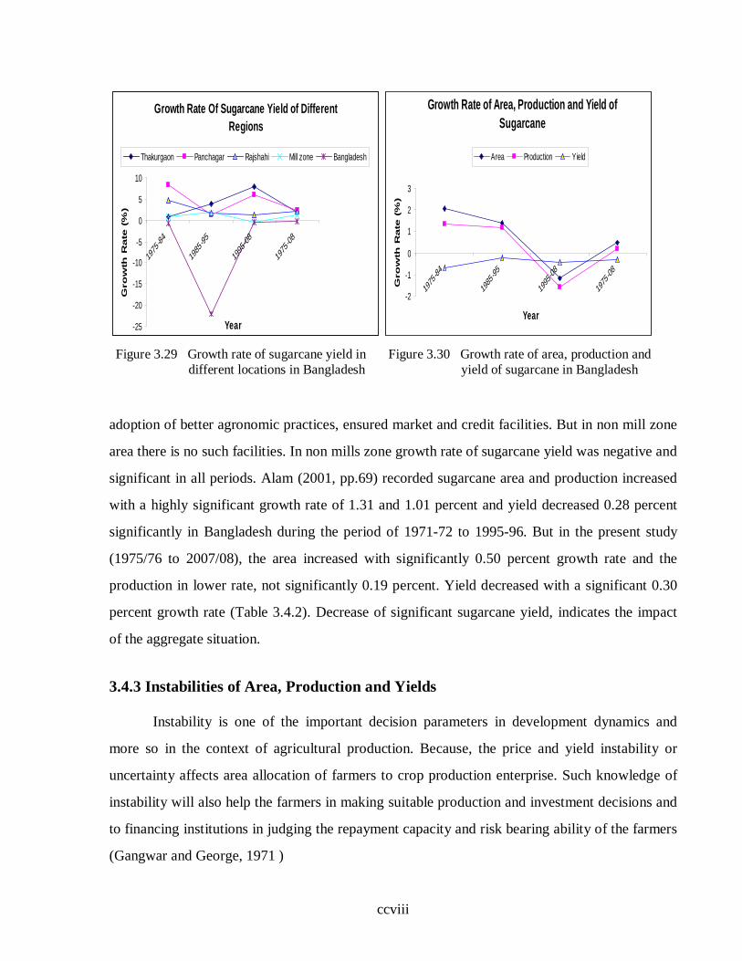
ccviii
Growth Rate Of Sugarcane Yield of Different Regions
-25
-20
-15
-10
-5
0
5
10
1975
-84
1985
-95
1995
-08
1975
-08
Year
Gro
wth
Rate
(%
)
Thakurgaon Panchagar Rajshahi Mill zone Bangladesh
Growth Rate of Area, Production and Yield of Sugarcane
-2
-1
0
1
2
3
1975
-84
1985
-95
1995
-08
1975
-08
Year
Gro
wth
Rate
(%
)
Area Production Yield
Figure 3.29 Growth rate of sugarcane yield in different locations in Bangladesh
Figure 3.30 Growth rate of area, production and yield of sugarcane in Bangladesh
adoption of better agronomic practices, ensured market and credit facilities. But in non mill zone
area there is no such facilities. In non mills zone growth rate of sugarcane yield was negative and
significant in all periods. Alam (2001, pp.69) recorded sugarcane area and production increased
with a highly significant growth rate of 1.31 and 1.01 percent and yield decreased 0.28 percent
significantly in Bangladesh during the period of 1971-72 to 1995-96. But in the present study
(1975/76 to 2007/08), the area increased with significantly 0.50 percent growth rate and the
production in lower rate, not significantly 0.19 percent. Yield decreased with a significant 0.30
percent growth rate (Table 3.4.2). Decrease of significant sugarcane yield, indicates the impact
of the aggregate situation.
3.4.3 Instabilities of Area, Production and Yields
Instability is one of the important decision parameters in development dynamics and
more so in the context of agricultural production. Because, the price and yield instability or
uncertainty affects area allocation of farmers to crop production enterprise. Such knowledge of
instability will also help the farmers in making suitable production and investment decisions and
to financing institutions in judging the repayment capacity and risk bearing ability of the farmers
(Gangwar and George, 1971 )

ccix
Instability plays a significant role in agricultural production. Farmers have to decide
which combination of crops they should choose to reduce income instability. Risks and
uncertainties adversely affect the optimization process of investment and production decisions in
agriculture. Yield variability is caused by weather fluctuations and diseases incidence. An
analysis of fluctuations in crop output, apart from growth, is of importance for understanding the
nature of food security, income stability variations in disposable income of the farmers (Kaushik,
1993).
In this section, attempt was made to examine the nature and degree of instability in area,
production and yield of sugarcane in different selected areas during the study period The stability
indices of area, production and yield of sugarcane for selected areas were estimated based on
coefficient of variation and coefficient of determination (R2) obtained from the fitted exponential
functions.
Instability Index (I) = (C.V2) × (1-R2)
Thus instability index captures both explained and unexplained variations of the concerned
variable and should better reflect the true instability situation. Instabilities of area, production,
yield and real price of sugarcane and some major crops were discussed. Moreover, area,
production and yield of sugarcane for different areas during 1975/76 to 2007/08 are discussed
below.
3.4.3.1 Instability of Area, Production, Yield and Prices of Sugarcane and Other Crops
Area instability of rice, wheat, potato, lentil and sugarcane was 7, 841, 1074, 956 and 48
respectively. The highest growth rate and instability index was found in potato area. Lower area
growth rate and instability was found in rice and sugarcane. The highest production instability
was found in wheat (1015), followed by lentil (998), potato (576) rice (53) and sugarcane (36).
Lentil attained the highest yield instability followed by wheat, potato rice and sugarcane. The
real price of potato occupied the highest instabilities followed by lentil, wheat, rice and
sugarcane during the study period (Table 3.4.3). Real price instability was higher than that of
area and yield for all crops. Price instability was caused mainly due to production instability. On

ccx
the other hand, wheat, potato and lentil price instability happened due to combined effect of area
and production instability during the study period ( Table 3.4.3). It is notable that yield instability
of rice and sugarcane was the minimum of all crops studied. So, production instability was
largely influenced by area instability during the entire period and area instability was influenced
by prices.
Table 3.4.3. Instabilities of area, production, yield and real prices of sugarcane and other crops (1975/76 to 2007/08)
Crops Instability index(I)*
Area Production Yield Real price
Rice 7 53 21 616
Wheat 841 1015 897 723
Potato 1074 576 148 9658
Lentil 956 998 1077 923
Sugarcane 48 36 8 149
* I= { (C.V.)2 * (1-R2)
3.4.3.2 Instability of Sugarcane Area in Different Locations
Long duration, unavailability of fertilizers and insecticides in proper time, profitability of
competing crops etc. reduced the land allocation for sugarcane cultivation. During the study
period (1975/76 to 2007/08) the instabilities in sugarcane area for Panchagar, Thakurgaon,
Rajshahi districts, all mills zone and whole Bangladesh were found 240, 395, 323, 173 and 48
percent respectively (Table 3.4.4). The area instability of sugarcane in Thakurgaon occupied the
top level followed by Rajshahi and Panchagar districts. Among the different districts Thakurgaon
was found to be the most risky for sugarcane cultivation. It was risky due to attack of pests and
diseases and less profitability than other locations. In Bangladesh sugarcane area occupied the
lowest instabilities in this study period. Bangladesh consists of mill zone and non mill zone.
There are 15 sugar mills under the mills zone and these mills are located in different districts. In
Bangladesh the highest and lowest area instabilities were 16 and 13 percent found in the period -
II and period - III respectively (Table 3.4.5). But in mill zone area the highest instabilities was
found 207 in period - I and the lowest 37 percent in period - II (Table 3.4.6). Within three
districts in different periods the highest sugarcane area instabilities was noted in Rajshahi 410

ccxi
percent in the period -I followed by 316 and 313 percent in Thakugaon during the period of I
and III respectively ( Table 3.4.7; 3.4.8 and 3.4.9). But the overall highest area instability was at
Thakurgaon (Table 3.4.1).
It is concluded that, in Bangladesh sugarcane area was more instable in period –III.
According to the opinions of the farmers, sugarcane cultivation was risky due to high initial
investment cost, long duration, high pest and diseases infestation, lower profitability than other
competing crops, closed market facilities, lower price and cane payment policies. It is also
concluded that in overall Bangladesh area, production and yield of sugarcane are less instable
than in any single district.
Table 3.4.4 Instability index of area, production and yield of sugarcane in different location during the period of 1975/76 to 2007/08.
Particulars Regions
Panchagar Thakurgaon Rajshahi Mill zone Bangladesh
Area
R2* 0.06 0.03 0.002 0.14 0.28 C.V. (%) 15.98 20.17 18.00 14.13 8.16 Instability index (I ) 240 395 323 173 48
Production
R2* 0.42 0.28 0.26 0.44 0.07 C.V. (%) 22.48 14.68 21.40 21.70 6.24 Instability index (I ) 293 155 339 262 36
Yield
R2* 0.38 0.46 0.38 0.59 0.48 C.V. (%) 20.20 23.15 19.42 13.75 3.94 Instability index (I ) 252 289 240 78 8
C.V. denotes coefficient of variation I implies Instability index, I = (C. V.)2 * (1-R2)
Table 3.4.5 Instability index of area, production and yield of sugarcane in Bangladesh in different period
Particulars Period – I
(1975/76 to 1984/85) Period – II
(1985/86 to 1994/95) Period- III
(1995/96 to 2007/08)
Area Production Yield Area Production Yield Area Production Yield
R2 0.73 0.49 0.61 0.53 0.45 0.07 0.87 0.79 0.26
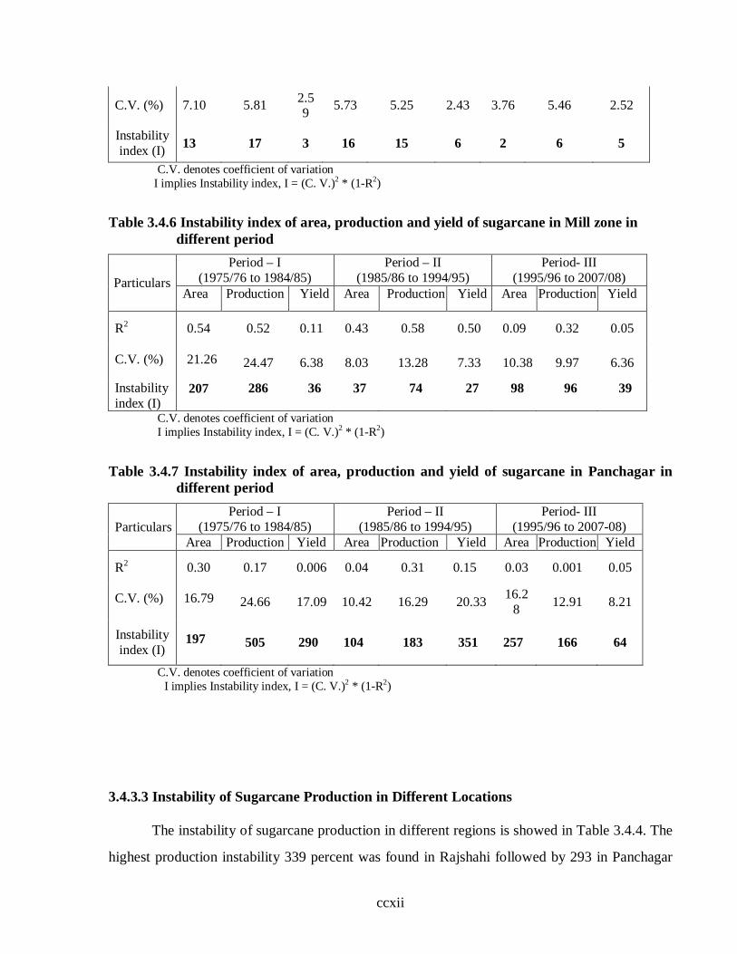
ccxii
C.V. (%) 7.10 5.81 2.59 5.73 5.25 2.43 3.76 5.46 2.52
Instability index (I) 13 17 3 16 15 6 2 6 5
C.V. denotes coefficient of variation I implies Instability index, I = (C. V.)2 * (1-R2)
Table 3.4.6 Instability index of area, production and yield of sugarcane in Mill zone in
different period
Particulars Period – I
(1975/76 to 1984/85) Period – II
(1985/86 to 1994/95) Period- III
(1995/96 to 2007/08) Area Production Yield Area Production Yield Area Production Yield
R2 0.54 0.52 0.11 0.43 0.58 0.50 0.09 0.32 0.05
C.V. (%) 21.26 24.47 6.38 8.03 13.28 7.33 10.38 9.97 6.36
Instability index (I)
207 286 36 37 74 27 98 96 39
C.V. denotes coefficient of variation I implies Instability index, I = (C. V.)2 * (1-R2)
Table 3.4.7 Instability index of area, production and yield of sugarcane in Panchagar in different period
Particulars Period – I
(1975/76 to 1984/85) Period – II
(1985/86 to 1994/95) Period- III
(1995/96 to 2007-08) Area Production Yield Area Production Yield Area Production Yield
R2 0.30 0.17 0.006 0.04 0.31 0.15 0.03 0.001 0.05
C.V. (%) 16.79 24.66 17.09 10.42 16.29 20.33 16.28 12.91 8.21
Instability index (I)
197 505 290 104 183 351 257 166 64
C.V. denotes coefficient of variation I implies Instability index, I = (C. V.)2 * (1-R2)
3.4.3.3 Instability of Sugarcane Production in Different Locations
The instability of sugarcane production in different regions is showed in Table 3.4.4. The
highest production instability 339 percent was found in Rajshahi followed by 293 in Panchagar

ccxiii
and 155 in percent Thakurgaon. The lowest production instability was noted in overall
Bangladesh (36%). Within Bangladesh the highest instability index of sugarcane production was
found 17 percent in period -I and the lowest was 6 percent in period-III. This high variation
instability index arises from variation in weather conditions, technological changes, pest and
diseases infestation, use of inputs and less profitability compared to other crops. This fluctuation
was not uniform among all other districts. In mill zone area the highest production instability
index was 286 percent in period -I and the lowest was 74 percent in the period - II. It was
concluded that production instability was highest in the period - I. Relative increase in the price
of fertilizer, insecticides and irrigation fuel cost due to the gradual withdrawal of government
subsidies were the plausible reasons for production instability of sugarcane in different locations
and different time periods. Since the fertilizer prices increased rapidly during the study period,
the farmers could not use optimum doses of fertilizers and then production decreased. As a
result, production instability increased.
3.4.3.4 Instability of Sugarcane Yields in Different Locations
The Yield instability of sugarcane in different districts/ regions was 252, 289, 240, 78 and
8 percent in Panchagar, Thakurgaon, Rajshahi, mill zones and whole Bangladesh (Table 3.4.4).
The highest yield instability was found in Thakurgaon and the lowest in overall Bangladesh. In
mill zone area the yield instabilities of period-I, II and III were 36 ,27 and 39 percent
respectively (Table 3.4.4). At Panchagar the highest yield instability was 290 in period I and the
lowest was 64 in period III (Table 3.4.7). At Thakurgaon yield instability index ranges from 255
(period I) to 520 (period II) percent (Table 3.4.8). It was 214, 263 and 59 percent in period I, II
and III at Rajshahi(Table 3.3.9). From the study it was revealed that yield instability index of
sugarcane was lower than production index. Wasim (1999, p 165) estimated the instabilities of
area, production and productivity of sugarcane were 0.07, 0.10 and 0.02 percent for the period
1982/83 to 1993/94. It indicated that the yield of sugarcane was more stable than area and
production. Adoption and expansion of newly released varieties and technologies were the
possible reason for achieving more stability in yield for sugarcane cultivation in the selected
districts.

ccxiv
Table 3.4.8.Instability index of area, production and yield of sugarcane in Thakurgaon in the different period
Partic-ulars
Period – I (1975/76 to 1984/85)
Period – II (1985/86 to 1994/95)
Period- III (1995/96 to 2007/08)
Area Production Yield Area Production Yield Area Production Yield R2 0.06 0.08 0.32 0.56 0.69 0.21 0.21 0.29 0.62 C.V. (%) 18.33 11.12 24.55 20.00 34.24 25.66 19.93 26.63 29.77 Instability index (I) 316 114 255 176 358 520 313 503 337
C.V. denotes coefficient of variation, I implies Instability index, I = (C. V.)2 * (1-R2)
Table 3.4.9 Instability index of area, production and yield of sugarcane in Rajshahi district
in the different period
Particulars
Period – I (1975/76 to 1984/85)
Period – II (1985/86 to 1994/95)
Period- III (1995-96 to 2007/08)
Area Production Yield Area Production Yield Area Production Yield
R2 0.70 0.64 0.54 0.11 0.02 0.08 0.07 0.12 0.03
C.V. 21 24.71 21.59 7.64 13.36 16.92 20.53 16.63 7.78
Instability index (I)
410 219 214 51 175 263 392 243 59 C.V. denotes coefficient of variation I implies Instability index, I = (C. V.)2 * (1-R2)
3.4.4 Summary of the Findings
In this section growth and instability of sugarcane and other agricultural crops were
estimated. High growth and high instability of area, production and yield were found in potato,
wheat and lentil. In sugarcane it was lower than other crops. The real price of those major
agricultural crops decreased, where it was decreased significantly in sugarcane during the period
of 1975/76 to 20007-08. The price of all agricultural crops depends on its market demands. But
in sugarcane it is determined by the govt. arbitrarily and it is ensured price. Area and production
of rice, wheat, potato and lentil increased significantly whereas, sugarcane area and production
did not increase significantly because it might be due to the lower price and less profitability
than other agricultural crops. Farmers could not sell it in the open market.

ccxv
Area and production of sugarcane in all mills zone increased significantly whereas, in
Panchagar, Rajshahi and overall Bangladesh area and production did not increase significantly
during the study period. Yield of all mills zone also increased significantly but in over all
Bangladesh it did not increase significantly. A major portion of sugarcane is produced in mill
zone area and sugar mill is the only one customer of sugarcane. In this area sugarcane production
and marketing is directly controlled by sugar mill. Growth rate in this area was higher due to the
availability of better irrigation facilities, adoption of modern technologies i.e. good seeds, plant
protection, adoption of better agronomic practices, ensured market and credit facilities. But in
non mill zone area there is no such facilities. In non mills zone growth rate of sugarcane yield
was negative and significant in the study period.
In Thakurgaon sugarcane area decreased significantly and its instability was too high
terms of instability index than Rajshahi and Panchagar district during the entire period.
Therefore, Thakurgaon area was found more risky for sugarcane cultivation. It was risky due to
frequent attack of pest and diseases and less profitability than other competing crops and low
technical, economic and allocative efficiency than other districts. Production instability of
sugarcane was the highest at Panchagar than Rajshahi, Thakurgaon. and over all Bangladesh,
where the highest growth rate in production was obtained at Panchagar. In over all Bangladesh
area, production and yield instability was 48, 36 and 8.
In order to improve the growth with stability in production, the important steps needed:
(i) New thrust on research must be in the direction of developing high yield- high sugar
content- cum high stability varieties suitable for rained as well as irrigated area and
also greater emphasis should be given for evolving short duration, drought, water
logging, salt tolerant and pest and disease resistant sugarcane varieties.
(ii) In order to check the diversion of land and other resources from sugarcane towards
competing crops, the comparative advantages need to be increased by improving the
yield and prices of sugarcane
(iii) Adequate credit facilities should also be provided to the farmers.
3.5 SUPPLY RESPONSE ANALYSIS OF SUGARCANE PRODUCTION

ccxvi
3.5.1. Introduction
Sugarcane is the second most important cash crop just after jute. It occupies 1.8 million
ha of land and it meets 28.55 percent (BBS, 2008) of the total requirements in Bangladesh.
Efforts are being made by the government towards boosting the sugarcane production to meet the
increasing demand for the growing population. Improved knowledge on the potential future
supply structure is needed for the appraisal of problems and potentialities in area development.
Accurate knowledge of supply is essential not only in formulating suitable set of policies but also
for better guidance and decision making to individual farmers. Estimation of supply responses
will help farmers in adjusting their production to projected prices to maximize their profit.
Price plays an important role in the selection of crops and generation of marketed surplus.
Generally higher prices are expected to result in a larger output. Prices are therefore, among the
most important determinants of the area under different crops. In economic analysis of the farm
supply response, price is considered to be critical economic factor that determines farmers'
production decisions.
According to response group of economists like Krishna (1963), Narain (1977) and
others farmers responded favorably to changes in prices. They argued that the response of
acreage to changes in relative price is a good indicator of the price responsiveness. Supply
response function provides useful information on the response to price and other economic
factors. Most of the supply response studies on food grains were confined to cereals only. For
sugarcane, however very few studies were available concerning the supply response. For this
purpose there is a need to identify the factors which influence the farmers' decision to allocate
more land to sugarcane. An attempt is, therefore made to examine the factors responsible for the
cultivation of sugarcane crop in Bangladesh. The sugarcane lagged year area, lagged sugarcane
price, lagged relative price, lagged relative yield, relative price risk, relative yield risk of
sugarcane, total irrigated area, lagged rainfall were used in the model. All variables prefixing
LN are in natural logarithm. The elasticity estimates obtained directly from the fitted data
through equation are short run elasticities of the variables. Long run elasticity was computed by

ccxvii
dividing the respective short run elasticity by the coefficient of the partial adjustment in the
equation.
3.5.2 Supply Response Models of Sugarcane in Bangladesh
The estimation of the acreage response function had revealed the existence of logical
relationships among the chosen variables. The coefficients and the associated ‘t’ statistics
showed that the variables have a significant effect on area allocation and presented in Table
3.5.1. The lagged area and relative price risk were found positive and significant at 1% level in
Bangladesh supply response model while the relative yield risk was positive and insignificant.
The coefficient of lagged sugarcane price and lagged relative price was found positive and
significant at 5 percent level whereas the lagged relative yield, total irrigation area and rainfall
were negative and significant at 1, 5, and 10 percent level respectively. The price elasticity of
sugarcane was 0.36 (Table 3.5.2) which is inelastic. The high values of the adjusted R2 and ‘F’
indicated good fit and the overall significance of the supply response functions. Explanatory
power of the equations is highly satisfactory because the value of adjusted R2 is 0.66 and F value
was 8.52 and significant at 1% level.
Lagged sugarcane area (At-1): The estimated coefficient of the lagged sugarcane area
was found to be consistent positive and highly significant. The significant effect of the lagged
sugarcane area may in part be explained by the farmer experience in a certain cropping pattern
and the existence of institutional constraints. This suggested that the sugarcane area of the
preceding year had positive influence on the sugarcane acreage. The short run elasticity of
sugarcane lagged area was 0.74 which indicates that farmers had a low rate of adjustment.
Lagged sugarcane price (Pt-1): Lagged price of sugarcane was found positive and
significant at 5 percent level. It implied that the farmers considered the previous year’s price of
sugarcane to allocate their land. It also indicated that when price of sugarcane increased, then the
sugarcane plantation of the next year directly increased.

ccxviii
Lagged relative price (RPt-1): Relative price, i.e., ratio of the price of the crop
concerned to the price of the competitive crop. Sugarcane is a long durable crop and it takes 12-
15 months from planting to harvesting. Here, wheat-jute cropping pattern were considered as a
competitive crops. The coefficient of lagged relative price of sugarcane was (0.07) positive and
significant at 5% level which implied that as the lagged one year relative price of competing crop
increased the area of sugarcane production would increase in the next year. It indicated that the
farmers considered relative price in making a decision about land allocation to this crop.
Lagged relative yield (RYt-1): Relative yield, i.e., ratio of the yield of sugarcane to the
yield of the competitive crop, here wheat-jute was considered as a competitive crop. The
coefficient of lagged relative yield of sugarcane was -0.22 and significant which revealed that 1
per cent increase in lagged relative yield would decrease the sugarcane area by 0.22 percent.
Relative price risk (RPR): Among different risk factors, the fluctuation in prices and
yield are the major ones. Being a cash crop, sugarcane is highly vulnerable to price changes.
How farmers have varied acreage under crops in response to the risks of variations in prices
needs to be explored. Therefore in this study, only the price risk or the standard deviation of
prices of sugarcane for the preceding year was used as a risk variable in the acreage response
model. This may be a sufficient way to incorporate risk particularly in the annual time series
model (Sidhu and Sidhu, 1988). The coefficients of relative price risk was (0.02) negative and
significant at 1% level which implied farmers’ risk averse response to price fluctuation. The
negative sign of the price risk variable indicated that sugarcane farmers appeared to be risk
lovers by putting less area under the crop.
Relative yield risk (RYR): The national yield level had almost stagnated in Bangladesh.
In this study, the yield risk is the standard deviation of sugarcane yield and the competing crops
(wheat-jute). The coefficient of relative yield risk was (0.004) negative but not significant which
implied that the relative yield risk had a negative impact on sugarcane area. The sugarcane
farmers exhibited yield risk adverse attitude as the yield risk variable came out with negative
sign.

ccxix
Irrigated area (Ir): The effect of irrigated area was found to be negative with an
elasticity coefficient of 0.04, which was significant at 5 percent level. When irrigated area
increased the area of sugarcane allocation decreased. Sugarcane is a long duration and cash cum
industrial crop. When the adequate irrigation facility are available the farmers were more
interested to cultivate wheat, rice and other short growing crops and then they allocated their
lands to the rice and other cereal crops. Lagged irrigated was selected as an appropriate
explanatory variable in sugarcane production. In Bangladesh sugarcane, wheat, rice and winter
vegetables were planted during the winter season. This showed that the farmers’ decision on how
much wheat, rice, sugarcane and other winter vegetables should be cultivated in winter season in
the year t was influenced by the irrigated areas in the previous year (t-1), rather than in year t.
Therefore, a one year lag in irrigated area was more realistic than without lag.
Table 3.5.1 Estimated parameters of Nerlovian Partial Adjustment Model of sugarcane in Bangladesh for the period from 1975/76 to 2007/08.
Variables Coefficients ‘t’ values
Constant 3.064* 2.783
Lagged area (At-1) 0.737* 4.668
Lagged sugarcane price (Pt-1) 0.361** 2.139
Lagged relative price (RPt-1) 0.067** 1.740
lagged relative yield (RYt-1) -0.219* -2.991
Relative price risk (RPR) -0.019* 2.625
Relative yield risk(RYR) -0.004 0.675
Irrigation (Ir) -0.04** -1.778
Lagged rainfall (Rt-1) -0.05*** -1.174
Adjusted R2 0.66
F 8.52*
d 2.06 Sources: BBS (1976-2008), BSFIC (1976-2008), DAM. *, ** and *** refers to significant at 1, 5 and 10 percent level respectively.

ccxx
Lagged rainfall (Rt-1): The coefficient of the lagged rainfall was (0.05) negative and
significant which implied that the rainfall of the previous year had a negative impact on
sugarcane area. Rainfall of the previous year increased the farmers’ allocated land for other short
duration crops like wheat, rice, pulses and other vegetables by decreasing sugarcane area.
3.5.3 Short and Long – Run Elasticity and coefficient of Adjustment
The long run elasticity was simply derived by dividing each corresponding short-
run elasticity by the coefficients of adjustment obtained from the model. The estimated short-run
and long- run elasticity of sugarcane production are presented in the Table 3.5.2. Price elasticity
of area response was found positive and significant. The long-run elasticity was the highest for
lagged sugarcane area (2.83). So, the long -run sugarcane supply response to lagged area was
greater than unity, or within the elastic range. The short-run and long -run price elasticity for
sugarcane lagged sugarcane price was 0.36, 1.39 respectively. This suggests that sugarcane was
not cultivated to meet farmers' subsistence needs. Nerlove (1958) mentioned that the full impact
of the distributed lag is called the long run response. Long run is the sufficient time when full
adjustment is possible. The full adjustment is possible when the supply is elastic that is why long
run sugarcane supply response to its lagged price was greater than unity, or within the elastic
range. The results of the study were, therefore, consistent with the Nerlove theory. Elastic supply
means sugarcane has many alternative crops. The short- run and long-run elasticity of lagged
relative price, lagged relative yield, relative price risk, relative yield risk, irrigated area and
lagged rainfall were 0.07, -0.22, 0.02, 0.004, -0.04, -0.05 and 0.26, -0.84, 0.07, 0.02, -0.169, -
0.20 respectively. The coefficient of adjustment turned out to be less than one, which signifies
the prevalence of area adjustment problems. The coefficients of adjustment is equal to 0.26 (1-
0.74 = 0.26), during the period of1975-76 to 2007-08 in sugarcane production (3.5.1).
Coefficients of adjustment 0.26, means that the Bangladeshi sugarcane farmers could adjust only
26 percent of the changes caused by fluctuations of exogenous variables within a production
period of one year.

ccxxi
Table 3.5.2 Estimated Short-run and Long-run Elasticity
Variables Short-run elasticity (SRE)
Long-run elasticity (LRE)
Coefficients of
adjustment
Lagged sugarcane area (At-1) 0.74* 2.83 0.26
Lagged sugarcane price((Pt-1)) 0.36** 1.39 Lagged relative price (RPt-1) 0.07** 0.26
Lagged relative yield (RYt-1) -0.22* -0.84 Relative price risk (RPR) -0.02* -0.07
Relative yield risk (RYR) -0.004 -0.015 Irrigated area -0.044 -0.169 Lagged rainfall (Rt-1) -0.052*** -0.20
Source: Derived from the Table 3.4.2
3.5.4 The test of Multicollinearity and Autocorrelation among the Explanatory
Variables
There is no correlation between explanatory variables of the regression analysis for the
sugarcane cultivation. Correlation among the explanatory variables were less than one for
sugarcane in Bangladesh, that is all the variables in the equation were free from the inter
correlation (Appendex-C).
To test the auto correlation Durbin -Watson test used and to remove autocorrelation 2nd
order autoregressive was done.
3.5.5 Summary of the Findings
Lagged sugarcane area was found to be positive and significant. Its main cause, as is
evident from the general psychology of the farmers, is that they follow tradition in making
decisions about raising different crops. They do not easily decide to reduce the area under the
ccxxii
crop in comparison with the area they showed in the preceding year. Lagged price and, lagged
relative price had the positive and significant sign. It Implies that the farmers should take into
consideration the own price and relative price along with its variations in making decisions about
the allocation of this crop. Relative price had the negative and significant impact indicated that
sugarcane farmers were risk lovers by putting less area under the crop. The coefficient of
adjustment in the equation implying that the sugarcane area in a particular year is far from
complete adjustment i.e. area adjustment problems are substantial as revealed by low (0.26)
coefficient of adjustment.
Finally, it should be noted that the conclusions drawn here are based on the data from
1975/76 to 2007/08. In the absence of any significant change in the sugarcane industry since
then, these conclusions are no doubt still valid. However further research could be undertaken at
a latter date to investigate whether there has been any significant structural change in sugarcane
area response since 2007/08.