A Study on Financial Distress of Selected Indian

Companies

A Thesis submitted to Gujarat Technological University

For the Award of

Doctor of Philosophy

In

Management

By

JAYA P. DAKHWANI

Enrolment No: 139997292004

Under supervision of

Dr. Keyur M Nayak

GUJARAT TECHNOLOGICAL UNIVERSITY

AHMEDABAD

February 2019

i

A Study on Financial Distress of Selected Indian

Companies

A Thesis submitted to Gujarat Technological University

For the Award of

Doctor of Philosophy

In

Management

By

JAYA P. DAKHWANI

Enrolment No.: 139997292004

Under supervision of

Dr. Keyur M Nayak

GUJARAT TECHNOLOGICAL UNIVERSITY

AHMEDABAD

February 2019

ii

© JAYA P. DAKHWANI

iii

DECLARATION

I declare that the thesis entitled “A Study of Financial Distress of selected Indian

Companies.” submitted by me for the degree of Doctor of Philosophy is the record of

research work carried out by me during the period September 2013 to May 2018 under the

supervision of Dr. Keyur M Nayak and this has not formed the basis for the award of any

degree, diploma, associate ship, fellowship, titles in this or any other University or other

institution of higher learning.

I further declare that the material obtained from other sources has been duly acknowledged

in the thesis. I shall be solely responsible for any plagiarism or other irregularities, if

noticed in the thesis.

Signature of the Research Scholar: …………………………… Date: ….………………

Name of Research Scholar: Jaya P. Dakhwani

Place: Navsari

iv

CERTIFICATE

I certify that the work incorporated in the thesis “A Study of Financial Distress of

selected Indian Companies.” submitted by Jaya P. Dakhwani was carried out by the

candidate under my supervision/guidance to the best of my knowledge:

i. the candidate has not submitted the same research work to any other institution for any

degree/diploma, associate ship, Fellowship or other similar titles

ii. the thesis submitted is a record of original research work done by the Research Scholar

during the period of study under my supervision, and

iii. the thesis represents independent research work on the part of the Research Scholar.

Signature of Supervisor: ……………………………… Date: ………………

Name of Supervisor: Dr. Keyur M Nayak

Place: Vapi

v

Originality Report Certificate

It is certified that PhD Thesis titled “A Study of Financial Distress of Selected Indian

Companies.” by Jaya P. Dakhwani has been examined by us. We undertake the following:

a. Thesis has significant new work / knowledge as compared already published or is under

consideration to be published elsewhere. No sentence, equation, diagram, table, paragraph

or section has been copied verbatim from previous work unless it is placed under quotation

marks and duly referenced.

b. The work presented is original and own work of the author (i.e. there is no plagiarism). No

ideas, processes, results or words of others have been presented as Author own work.

c. There is no fabrication of data or results which have been compiled / analyzed.

d. There is no falsification by manipulating research materials, equipment or processes, or

changing or omitting data or results such that the research is not accurately represented in

the research record.

e. The thesis has been checked using Turnitin (copy of originality report attached) and found

within limits as per GTU Plagiarism Policy and instructions issued from time to time (i.e.

permitted similarity index <=25%).

Signature of the Research Scholar: …………………………… Date: …………...………

Name of Research Scholar: Jaya P. Dakhwani

Place: Navsari

Signature of Supervisor: ……………………………… Date: …………………

Name of Supervisor: Dr. Keyur M Nayak

Place: Vapi

vi

PhD THESIS Non-Exclusive License to

GUJARAT TECHNOLOGICAL UNIVERSITY

In consideration of being a PhD Research Scholar at GTU and in the interests of the

facilitation of researchat GTU and elsewhere, I, Jaya P. Dakhwani having Enrollment No.

139997292004 hereby grant a non-exclusive, royalty free and perpetual license to GTU on

the following terms:

a) GTU is permitted to archive, reproduce and distribute my thesis, in whole or in part, and/or

my abstract, in whole or in part ( referred to collectively as the “Work”) anywhere in the

world, for non-commercial purposes, in all forms of media;

b) GTU is permitted to authorize, sub-lease, sub-contract or procure any of the acts

mentioned in paragraph (a);

c) GTU is authorized to submit the Work at any National / International Library, under the

authority of their “Thesis Non-Exclusive License”;

d) The Universal Copyright Notice (©) shall appear on all copies made under the authority of

this license;

e) I undertake to submit my thesis, through my University, to any Library and Archives. Any

abstract submitted with the thesis will be considered to form part of the thesis.

f) I represent that my thesis is my original work, does not infringe any rights of others,

including privacy rights, and that I have the right to make the grant conferred by this non-

exclusive license.

g) If third party copyrighted material was included in my thesis for which, under the terms of

the Copyright Act, written permission from the copyright owners is required, I have

obtained such permission from the copyright owners to do the acts mentioned in paragraph

(a) above for the full term of copyright protection.

h) I retain copyright ownership and moral rights in my thesis, and may deal with the

copyright in my thesis, in any way consistent with rights granted by me to myUniversity in

this non-exclusive license.

vii

i) I further promise to inform any person to whom I may hereafter assign or license my

copyright in my thesis of the rights granted by me to my University in this non-exclusive

license.

j) I am aware of and agree to accept the conditions and regulations of PhD including all

policy matters related to authorship and plagiarism.

Signature of the Research Scholar:

Name of Research Scholar: Jaya P. Dakhwani

Date: Place: Navsari

Signature of Supervisor:

Name of Supervisor: Dr. Keyur M Nayak

Date: Place: Vapi

Seal:

viii

Thesis Approval Form

The viva-voce of the PhD Thesis submitted by Jaya P. Dakhwani (Enrolment No.

139997292004) entitled “A Study of Financial Distress of selected Indian Companies” was

conducted on ……………………………………. At Gujarat Technological University.

(Please tick any one of the following option)

The performance of the candidate was satisfactory. We recommend that he be awarded the PhD

degree.

Any further modifications in research work recommended by the panel after 3 months from the

date of first viva-voce upon request of the Supervisor or request of Independent Research

Scholar after which viva-voce can be re-conducted by the same panel again.

(Briefly specify the modifications suggested by the panel)

The performance of the candidate was unsatisfactory. We recommend that he should not be

awarded the PhD degree.

(The panel must give justifications for rejecting the research work)

------------------------------------------------------Name and Signature of Supervisor with Seal

-------------------------------------------------------1) (External Examiner 1) Name and Signature

-------------------------------------------------------2) (External Examiner 2) Name and Signature

-------------------------------------------------------3) (External Examiner 3) Name and Signature

ix

ABSTRACT

Financial Distress is the stage before bankruptcy; financial distress is the late stage of corporate

decline where firm faces lack of liquidity. It is the stage where the firm finds difficulty in making

payments to its creditors and other stake holders. If attention is not paid or such situation is not

relieved, it will result in bankruptcy. The area of distress prediction is of high economic

importance, as it affects huge section of society.Thus early recognisation of it helps firm to get

relaxation from its danger zone.

The prediction of financial distress and corporate insolvency has been the matter of talk

among the academic literature and professional researcher throughout the world. A lot of

publication has been issued and lots of results have been represented. New techniques and

methodology are created constantly. But very few studies are conducted considering Indian

context due to limitation of scare of information available. Raising rate of in-debtness of Indian

Companies directing towards corporate leverage is one of the leading motivating factor for

researcher. Therefore the basic purpose of the research is to come up with the model that can

estimate the probability of failure or distress of Indian companies in next year by evaluating its

occurrence of failure using multiple discriminant analysis. Researcher has re estimated the

coefficient for developing the model.

The research focus on comparison of financial position of the selected companies through

financial information obtained from respective companies financial statement by using Z score,

O score and newly framed model. Initially researcher test the models with original established

model and with the help of logistic regression, she tries to examine role of accounting ratio.

The outcome of the study is when the discriminant functions were used to predict from the five

variables, 84% of the original grouped cases were correctly reclassified back into their original

categories. Using Logistic regression at the first step, the bankrupt category is classified 67% and

non bankrupt category by 91% correctly. The model increase correct classification as it increases

the steps. At the forth step, the bankrupt category is 100% and not bankrupt category by 100%

correctly classified. The overall correct classification of model is 100 %.

x

Acknowledgement

Completion of PhD thesis is a dream comes true. I could achieve this dream with the help of

many people, I would like to thank and acknowledge all those who have been involved in

making of my doctoral research.

First and foremost I would like to thank my supervisor Dr. Keyur M Nayakfor his valuable

guidance throughout my research and for supporting me whenever I needed his help in all

aspects. I would also thank my co-supervisor Dr Agim Mamuti, Associate Professor of

Accounting, College of Business Administration (COBA) for giving his prompt and positive

feedback every time.

I would also like to thanks my Doctoral Progress Committee members, Dr. Jaydip Chaudhry

and Dr. Vinod Patel, Dean and Professors, DBIM Surat for reviewing my progress continuously

and giving me their valuable feedback on my research topic and giving me permission for

conducting my open seminar at DBIM, Surat.

I would also like to thank knowledgeable experts at Research Review Week, and others who

have critically evaluated my research progress and have added precious inputs to my research

work.

I would also thanks Management of Agrawal Education Foundation, Navsari, for providing

me NOC for pursuing PhD from GTU and supported me without any obstacles.

Thanks to the GTU PhD Admin staff for their good cooperation and prompt replies to any of our

queries. Thanks to Dr. Sham Sachinwala, who has been very kind enough to support and

motivate me throughout my research work by critically reviewing my work. He has helped me in

identification of gaps and many more things.

I would also thank my colleague Dr.Shital Padhiyar for always motivating me towards the

early completion of PhD. I am also grateful to my colleague Miss Dhrasti Patel and Jhanvi

Khamdar for attending my open seminar.

xi

I would also like to thanks my parents for motivating me in every aspects of life. Last but not

the least, my heartfelt appreciation to my loving husband Mr. Nikesh Vadhvani and my sweet

child Kabir. Without their continuous support and motivation I would never had completed my

research.

xii

Table of ContentsDECLARATION .............................................................................................................................................. iii

CERTIFICATE ................................................................................................................................................. iv

Originality Report Certificate ........................................................................................................................ v

PhD THESIS Non-Exclusive License............................................................................................................... vi

Thesis Approval Form ................................................................................................................................ viii

ABSTRACT..................................................................................................................................................... ix

Acknowledgement ........................................................................................................................................ x

List of Abbreviation......................................................................................................................................xv

List of figures..............................................................................................................................................xvii

List of Tables .............................................................................................................................................xviii

CHAPTER 1 .................................................................................................................................................... 1

Introduction .................................................................................................................................................. 1

1 Introduction .......................................................................................................................................... 1

1.1 Background ...................................................................................................................................1

1.2 Motivation of Research................................................................................................................. 3

1.3 Financial Distress........................................................................................................................... 4

1.3.1 Different terminologies and definition: ................................................................................ 4

1.3.2 Perception related to Financial Distress: .............................................................................. 5

1.3.3 Sign of Financial Distress....................................................................................................... 6

1.3.4 Factors that leads to Financial Distress................................................................................. 7

1.3.5 Direct and Indirect cost of Financial Distress........................................................................ 9

1.3.6 Importance of Financial Distress Analysis.............................................................................9

1.3.7 Consequences of Financial Distress: ...................................................................................10

1.4 Bankruptcy Prediction models:...................................................................................................10

1.4.1 Accounting Based Model: ...................................................................................................11

1.4.2 Market Based Model:.......................................................................................................... 11

1.5 Different financial distress studies:.............................................................................................12

1.5.1 Edward Altman’s Model:.....................................................................................................12

1.5.2 Ohlson Model:.....................................................................................................................15

1.6 Financial Distress in India:...........................................................................................................16

xiii

1.7 Insolvency and Bankruptcy Code, 2016......................................................................................19

1.8 Original Contribution by the study .............................................................................................20

1.9 Presentation of the study ...........................................................................................................20

2 Literature Review................................................................................................................................22

2.1 Introduction ................................................................................................................................22

2.2 Literature related to different accounting and marketing based models. .................................23

2.3 Gaps Identified............................................................................................................................38

3 Research Methodology .......................................................................................................................39

3.1 Introduction ................................................................................................................................39

3.2 Problem Statement.....................................................................................................................39

3.3 Significance of Study ...................................................................................................................39

3.4 Definition of problem..................................................................................................................40

3.5 Objectives....................................................................................................................................40

3.6 Scope of the work .......................................................................................................................41

3.7 Research Design.......................................................................................................................... 41

3.7.1 Universe ..............................................................................................................................41

3.7.2 Sampling Frame...................................................................................................................41

3.7.3 Sample size.......................................................................................................................... 41

3.7.4 Sampling Techniques ..........................................................................................................41

3.7.5 Sources of Data Collection ..................................................................................................41

3.8 Statistical Tools & Techniques for bankruptcy prediction models ............................................. 42

3.8.1 Multiple Discriminant Analysis: .......................................................................................... 42

3.8.2 Logistic Regression:.............................................................................................................42

3.9 Limitations of the study ..............................................................................................................44

4 Data Analysis and Interpretation ........................................................................................................45

4.1 Edward Altman Model ................................................................................................................ 45

4.1.1 Result based on Altman Z score Model .............................................................................. 46

4.1.2 Descriptive Statistics for explanatory variables ..................................................................49

Table 7: Descriptive Statistics for explanatory variables .................................................................... 49

4.1.3 One way ANOVA .................................................................................................................49

4.1.4 Discriminant Analysis ..........................................................................................................63

4.2 Discriminant Function:................................................................................................................ 71

xiv

4.2.1 Classification Results...........................................................................................................71

4.2.2 Analysis of Result ................................................................................................................ 72

4.3 Ohlson Model..............................................................................................................................73

4.3.1 Description of Ohlson O score Variables ............................................................................74

4.3.2 Descriptive Statistics for studied Models............................................................................82

4.3.3 Descriptive Statistics ...........................................................................................................82

4.4 Logistic Regression (from Ohlson model) ...................................................................................83

4.4.1 Omnibus Tests of Model Coefficients .................................................................................84

4.4.2 Summary of the model .......................................................................................................84

4.4.3 Hosmer and Lemeshow Test...............................................................................................85

4.4.4 Classification Matrix for the bankruptcy model with Ohlson Model.................................. 85

4.4.5 Descriptive statistics for the estimation sample.................................................................86

4.4.6 Classification matrix for the bankruptcy model (Ohlson Model) with original statistical technique ............................................................................................................................................88

4.4.7 Classification matrix for the bankruptcy model (Altman Model) with original statistical technique ............................................................................................................................................88

4.4.8 Overall Accuracy of the Model............................................................................................89

5 Findings and Conclusion...................................................................................................................... 90

5.1 Findings .......................................................................................................................................90

5.1.1 ANOVA ................................................................................................................................90

5.1.2 Post Hoc Tests .....................................................................................................................90

5.1.3 Discriminant Analysis ..........................................................................................................91

5.1.4 Logistic Regression..............................................................................................................91

5.2 Conclusion...................................................................................................................................91

5.3 Achievements with respect to Objectives ..................................................................................92

5.4 Original Contribution made by the thesis...................................................................................94

5.5 Future Scope of the study:..........................................................................................................94

xv

List of AbbreviationANOVA Analysis of VarianceAZ Altman Z-scoreBIFR Board for Industrial and Financial ReconstructionBPNN Back Prorogation neural NetworksBSE Bombay Stock ExchangeCA Current AssetsCAGR Compound Annual Growth RateCF Cash-FlowCPM Conditional Probability ModelCR Current Ratio (current assets / current liabilities)DA Discriminant AnalysisEBIT Earnings Before Interest and TaxFMCG Fast Moving Consuming GoodsGDP Gross Domestic ProductGNP Gross National ProductGNP Gross National ProductIBC Insolvency and Bankruptcy Code, 2016IMF International Monetary FundINTWO One if NI was negative for the last two years, zero otherwiseISE Irish Stock ExchangeLA Logistic AnalysisLDF Logistic Distribution FunctionLMDA Linear Multivariate (or Multiple) Discriminant AnalysisLSE London Stock ExchangeMDA Multivariate (or Multiple) Discriminant AnalysisMDA Multivariate (or Multiple) Discriminant AnalysisNCLT National Company Law TribunalNI Net IncomeNI Net IncomeNN Neural NetworkNPA Non Performing AssetNSE National Stock Exchange of India Ltd.OCP Operating Cash flow

xvi

OENEG Dummy variable. One if total liabilities exceeds total assets, zero otherwiseOL Ohlson’s logit modelQR Quick Ratio (cash or cash equivalents / current liabilities)ROC Receiver Operating CharacteristicROI Return on InvestmentRPA Robotic Process AutomationSAIL Steel Authority of India LimitedSICA Sick Industrial Companies ActSVM Support Vector MachineTA Total AssetsTCP Traditional cash flowTL Total LiabilitiesTLTA Total Liabilities divided by Total AssetsUK United Kingdom (of Great Britain and Northern Ireland)US United States (of America)WCTA Working Capital divided by Total Assets

xvii

List of figuresFigure 1 : Different Terminologies and Definition.......................................................................................5Figure 2: Bankruptcy Prediction models.................................................................................................... 11Figure 3: Issue concerning Resolution .......................................................................................................17Figure 4: Snapshot of Insolvency and Bankruptcy Code-2016 ..................................................................18Figure 5: Bankruptcy and Insolvency code-Idea to Implementation..........................................................19Figure 6: Features of Insolvency and Bankruptcy code, 2016 ................................................................... 20

xviii

List of TablesTable 1: Discriminant Function Variables for different versions of Altman Model................................... 13Table 2: Z-Score Cutoff Points ...................................................................................................................14Table 3 Overview of the sickness prediction models formulated by earlier Researchers...........................37Table 4: Logistic Regression – Description of Terms.................................................................................43Table 5: Description of the ratio used by Altman .......................................................................................46Table 6: Results Based on Altman Z Score Model......................................................................................47Table 7: Descriptive Statistics for explanatory variables ............................................................................49Table 8: Descriptive Statistic......................................................................................................................50Table 9: Test of Homogeneity of Variances................................................................................................51Table 10: Result of ANOVA.......................................................................................................................... 51Table 11: Post Hoc Tests ............................................................................................................................52Table 12: Descriptive statistic ....................................................................................................................53Table 13 : Test of Homogeneity of Variances.............................................................................................54Table 14: Result of ANOVA ........................................................................................................................54Table 15: Post Hoc Tests ............................................................................................................................55Table 16: Descriptive Statistic ....................................................................................................................56Table 17: Test of Homogeneity of Variances..............................................................................................56Table 18: Robust Tests of Equality of Means .............................................................................................57Table 19: Post Hoc Tests ............................................................................................................................58Table 20: Descriptive Statistic ....................................................................................................................59Table 21: Test of Homogeneity of Variances..............................................................................................59Table 22: Robust Tests of Equality of Means .............................................................................................60Table 23: Post Hoc Tests ............................................................................................................................60Table 24: Descriptive Statistic ....................................................................................................................61Table 25: Test of Homogeneity of Variances..............................................................................................62Table 26: Robust Tests of Equality of Means .............................................................................................62Table 27: Post Hoc Tests ............................................................................................................................63Table 28: Descriptions................................................................................................................................64Table 29: Group Statistics .......................................................................................................................... 64Table 30: Tests of Equality of Group Means ..............................................................................................65Table 31 : Pooled Within-Groups Matrices................................................................................................66Table 32: Log Determinants .......................................................................................................................67Table 33: Box M Test Results .....................................................................................................................67Table 34: Summary of Canonical Discriminant Functions ........................................................................68Table 35: Test of Equality of Variance .......................................................................................................68Table 36: Standardized Canonical Discriminant Function Coefficients ....................................................69

xix

Table 37 : Structure Matrix ........................................................................................................................70Table 38 : Canonical Discriminant Function Coefficients .........................................................................70Table 39: Classification Results .................................................................................................................71Table 40 : Analysis of Result ......................................................................................................................72Table 41: Description of Ohlson O score Variables...................................................................................75Table 42: Result based on Ohlson O score Model......................................................................................78Table 43 Descriptive Statistics for studied Models.....................................................................................82Table 44: Omnibus Tests of Model Coefficients ......................................................................................... 84Table 45: Model Summary.......................................................................................................................... 84Table 46 : Hosmer and Lemeshow Test ......................................................................................................85Table 47: Classification Matrix for the bankruptcy model with Ohlson Model .........................................85Table 48: Descriptive statistics for the estimation sample .........................................................................86Table 49: Classification matrix for the bankruptcy model using Ohlson Model with original statistical technique .....................................................................................................................................................88Table 50 : Classification matrix for the bankruptcy model using Altman Model with original statistical technique .....................................................................................................................................................88Table 51: Overall Accuracy of the Model...................................................................................................89Table 52: Achievements with respect to Objectives....................................................................................92Table 53: Differentiating Factors between the Developed Models and Proposed Model..........................94

Introduction

1

CHAPTER 1

Introduction

1 Introduction

1.1 Background

Financial Distress is a very actual subject in the financial world. The prediction of financial

distress and corporate insolvency has been the matter of talk among the academic literature

and professional researcher throughout the world. A lot of publication has been issued and lots

of results have been represented. New techniques and methodology are created constantly.

Continuous entry and exit is the base of competition among the firms in market. Entry and exit

of the firm may be the reason of collapse or introduction of some product, emergence of new

industry creating opportunities and downfall of some of the industry causing shutdown, raises

or shortage of some of the resources etc. Theoretically, in highly competitive market, concept

like financial distress, bankruptcy, insolvency hardly exists. Financial distress is a temporary

process which is the matter of perception of the participants when they are not able to cope up

with the market due to slowdown of demand of the product, production from obsolete

technology or due to inefficient management, inefficient resource utilisation, inefficient

financial structure etc. Financial Distress is having various series of definition in its literature.

Dynamic nature of financial distress passes through different stages and each of the stages

having different characteristics which contribute differently towards business failure.

Financial Distress is the stage before bankruptcy; Financial Distress is the stage where

the firm finds itself in difficult situation to pay obligation to its creditors and other stake

holders. The firm is in danger zone, if attention is not paid, such situation is not relieved, if

firm does not take any corrective step to stop it from affected by its adverse effect, the result

Introduction

2

will be bankruptcy. Thus it saves firms from entering into danger zone by providing early

warning signals. As irrespective of shape of stone, when it is thrown in the water, ripples

spread out as soon as it touches the surface of the water and becomes its effect are far reaching

which one may not even know. Similarly if company defaults or become insolvents for any of

the reason, its effects are may not be known to different stakeholders, to society, to wider

economy, it may be widespread also. There can be variety of reason of Financial Distress, for

e.g.: economic slowdown, demand devastation, shrinking market capitalization, technological

failure, industry failure , problem with selection of location, poor performance of firm, under

and over capitalization, inappropriate capital structure as well as downturn stage of Business

cycle etc. All these factors together make the business indefensible. The timely predictions of

failure of corporate business have gained huge importance because of its widespread effect

over society. As per “Domino effect” cumulative insolvency produced due to sets up of

corporate insolvent of one firm. Thus financial restructuring becomes obligatory for

financially sick companies. Infusion of capital is one of the alternatives to alleviate financial

distress.

According to report prepared by (peter Lindner, December 2014) in International

Monetary Fund (IMF) regarding the financial status in Indian corporate, Indian firms are

facing severe problems in repayment of Loans due to decline in profitability and high level of

leverage. This result in failure of the firms which further affects the stakeholders namely

employees in terms of losing the job and creditors losing their capital.

Financial Distress is a global issue; different countries have different ways to deal with

companies suffering financial distress. According to(Antonio E. Bernardo, 2015)all the

financial distressed firms in US, are filed under chapter 11 of Bankruptcy code, whereas there

is no such specific law regarding this in UK, it is usually considered as liquidation. Before in

India there was no specific policy to deal with financial distress firms, the rules were covered

under the Companies Act 1956 and the Sick industrial Companies Act, 1985, and were

referred to BIFR. But recently single law have been declared to deal with financial distress

after passing of insolvency and bankruptcy code bill1.According to the survey done by World

Bank (Doing Business in 2005- Indian Regional Profile) has concluded that compare to other

1(Bapat V. &., 2016)

Introduction

3

countries which takes 1 to 6 years to liquidate whereby in India it takes 10 years.2Jardi and

Severin (2010) in their paper studied that failure of a business is not a sudden event, it passes

through different phase, and if early warning signals are detected, the more time one can

dedicate for exploration of its solution. Therefore, forecasting of financial distress is

significantly important. Forecasting techniques will be able to provide early warning signal

and will provide adequate time lag for taking remedial action and to correct the stage of

financial distress. Such prediction will help lending banks not to finance the firms that are

suppose to fail in near future, even the investors can avert capital loss by not investing in the

companies which are under financial distressed zone.

The Traditional analysis of ratios has been used to spot the financial and operative

difficulties faced by different firms, as financial information is the reflection of firm’s

performance, many studies focus on the financial analysis. Varieties of the models have been

introduced such as univariate discriminant analysis, multivariate discriminant analysis, binary

logistic, logistic regression etc. Altman is considered as an initiator of the studies, as he was

the first to use statistical method to explore bankruptcy and then it became widespread. In his

model, he used financial statement data to depict relationship between risk factor and firm’s

failure. In India also few studies have come up with different models. L.C Gupta, in his study

on “financial ratio for signalling corporate failure” mentioned that in predicting corporate

financial status, profitability ratio have more potential. Along with it, he also further added

that companies with low equity base are more prone to financially sick. Research has been

continued presenting different models; some of them have good accuracy for predicting

bankruptcy.

1.2 Motivation of Research

Corporate financial distress prediction is vital issue throughout the globe, India is not

exceptional. Booming rate of bankruptcy of Indian Companies directing towards creation of

debt for corporate survival is one of the leading fascinating factor for researcher. Research is

attempted to follow proactive approach for companies to prevent financial distress and take

corrective action, if financial distress is predicted. As early detection of potential failure in

2(Rohit Bansal, 2017)

Introduction

4

companies could provide the parties concerned with early indication that could enable

management to take preventive action. This model can also be used by lenders and banks to

know the future status of the companies before extending the loan to prevent NPA problem.

Therefore the basic purpose of the research is to come up with the model that can estimate the

probability of failure or distress of Indian companies in near future by evaluating its

occurrence of failure using multiple discriminant analysis and logit analysis.

1.3 Financial Distress

Financial Distress is a generic phrase that expressed winding or weakening financial situation

of the firm. In general the term Financial Distress is state of affairs as when company is unable

to meet its commitment on time and to the full extent. These denote negative financial

situation of the company which is the result of poor performance or the situation arising from

of lack of liquidity on temporary basis. It is the situation where companies’ cash flows are not

adequate enough to meet its obligation, or faces difficulties in paying off its obligation to

various stakeholders. Poor sales, poor profits, struggling to break even, inferior quality of

services and products etc are the symptoms indicating problematic situation for companies. If

this situation prevails for a longer period of time, this will not take time for the companies

going bankrupt. There are chances that the moral of people working with company may go

down because of stress of losing their jobs if companies default. Big customers may cancel

their order in anticipation of that their order will not be met on time. Even the

creditworthiness of the firms will be adversely affected which ultimately lead to limited

availability of funds from the market and will result in company failure.

1.3.1 Different terminologies and definition:

Economic or financial failure conveys different meaning to different people so the purpose

behind clarification of different concepts and terminologies are to shed light on the gist of the

terms applied. Default, distress, liquidation, industrial sickness, corporate failure, insolvency

and bankrupt are common terms that are used in the literature defining business failure. All

these terms are perceptibly different though these terms are used interchangeably or denote

similar. In fact literature related to prediction of failure uses almost the same process for

analysis irrespective of whether the model is for predicting financial distress or for prediction

Introduction

5

of bankruptcy. It may seem to be easy to define but bit difficult to define. It is relative concept

difficult to find in absolute term in concrete world. Different researchers and scholars implicit,

measured, interpreted differently because of its numerous forms at particular point of time.

1.3.2 Perception related to Financial Distress:

Difference in perceptions among various parties ‘to the term financial distress conveys

different meaning. For instance, it refers to detrimental or unhealthy organization for general

community, it is non- profitable enterprise for investors, for industrialist it is disappointing

unit, for lenders or creditors it is doubtful debtors or weak borrowers who cannot pay its dues

on time. For government it is source of disputes, for technologist it is victim of technological

change, for an employee it is a bad employer and for country as a whole it is source of wastage

of technical and human resources. The variation in perception of financial distress deserves a

well structured definition, which will embrace all pre-requisites.3

Figure 1 : Different Terminologies and Definition

Source:https://www.civilsdaily.com/story/insolvency-and-bankruptcy-code

3 Financial Statement analysis by Gokul Singh chapter 7 Distress analysis

Financial Distress:

It is a state in which firm face financial difficulties in

meeting its obligation at its current pace

Liquidation:

It is process of winding up a company that

follows after bankruptcy

Bankruptcy:

It preceeds liquidation when person is legally

declared as incapable of paying their dues and

obligation.

Introduction

6

1.3.2.1 Default, Insolvency and Financial Distress

Default is a blameless event result of deferred payment and poor collection efforts towards

debtors.

Insolvency is the condition when firm or entity fails to meet its obligation on account of lack

of liquidity. It is a stage where firm is provoked towards the filing of bankruptcy.

Financial Distress is the late stage of corporate decline featuring inadequate income and

inadequate liquid asset and if not recovered, it may result in bankruptcy.

1.3.2.2 Bankruptcy and Financial Distress

Bankruptcy is another financial concept that is used interchangeably with the word

Financial Distress in many of the literature of empirical studies. But in actual sense both the

terminology are different. In general bankruptcy is conclusive event of failed firms.

Bankruptcy is the next stage that comes after if financial distress is not recovered. It is a

formal declaration to the court in form of petition regarding liquidation of assets. Thus

bankruptcy is the last choice of Businessman. As all the companies do not go for bankruptcy,

taking sample size from it is limited. So for flexibility, many of the researchers take sample

size from financial distress4 . India has coined her own terminology as industrial sickness or

corporate sickness. The term financial distress and bankruptcy has been used interchangeably

by the researcher in this study.

1.3.3 Sign of Financial Distress

The indication starts with poor profits where companies are struggling for break even to

sustain itself from internal funds. Companies face difficulty in raising fund internally and are

forced to raise capital externally. Limiting to access to funds result in poor financial health. On

account of these tremendous difficulties, companies may decide to shut down the business.

4(Aktan, 2011)

Introduction

7

The benefits of acknowledging of such information in advance will help people those who are

directly or indirectly related with the enterprise. The above mentioned situation lowers the

creditworthiness with stakeholders.

1.3.4 Factors that leads to Financial Distress

1. Insufficient Accounting Practice:

Inadequacy of maintaining advanced accounting techniques or practice due to lack of

knowledge is one of the reasons of failure of business. Simply recording of numbers

after the fact will not enable one to spot trends and will lead to business failure as it

will not help to avoid problem.

2. Unrealistic Budgeting and pricing:

Preparing budget simply based on unrealistic data can lead to financial struggle that

might not be able to overcome.

3. Inadequate Cash Flow:

The statement of cash flow is financial statement that helps company to know situation

of cash generated and spend in business; it is summarised statement showing cash

inflow and outflow which is basically receipt and payment.

4. Poor Management:

Poor management means poor debt management which create a financial problem.

Missing loan payments can damage the credit scoring, lead to a loss of credit and

decrease ability to get new credit and which further create debt cycle.

5. Lack of Innovation:

In the era of Globalisation, those companies who fail to update or innovate are fore

sure will be in trouble leading to financial distress.

6. Declining sales:

Saturated or declining sales and high costs are the two of the most apparent reasons of

businesses suffering from financial distress as today one is more prone to increase

profit instead of increasing sales. Decrease in sales drain company cash, this will lead

to cash crisis as company run out of cash.

7. Company’s inability to retain key staff:

Introduction

8

Employee’s retention has become a challenging issue for every industry. Business is in

trouble or are red flag if there is major change in employee’s turnover specifically

talent retention of key personnel are slipping out of the company.

The above discussed factors are having direct impact on business and are the factors

internal to the organisation and are to some extent controllable. Along with these

factors, there are other factors also which are outside to the business known as external

factors also called remote factors that cause financial distress which are beyond the

business and their effects are general to industry irrespective of firm. These are the

factors which cannot be prevented but with effective measure it can be managed. These

are the different Business environment namely:

1. Social Environment:

There may be withdrawal of major customers due to change in taste and Preference of

resulting into decline in sale. Ignoring the taboos and culture specifically when business

operating globally can prove to be the biggest reason of failure.

2. Economic Environment:

These are the environment that are related to economic condition and policy of the

country that affects due to change in Government policy regarding taxation, change in

Inflation rate, lending policy of Financial Institutes, monetary policy, fiscal policy,

exchange rate fluctuation custom duties, import export duties etc.

3. Legal Environment:

Stressed relationship of the ruling political parties with the government of other

countries, bankruptcy law, commercial law, Imposition of Quota system, Import Export

tariff etc. are subject to penalties if not followed, and thus spoil the reputation and

ultimately business.

4. Technological Environment:

Outbreak of new technology, obsoleteness of existing technology, decrease in

production capacity due to depreciation of machinery, rejection of the large

consignment by customers due to new entrants in the market with latest technology are

the composition of these environment. Incapability of adaptation to technological

Introduction

9

changes or wrong estimation or uncertainty of economic direction can easily put an end

to the company.

5. Natural Environment :

Losses due to floods, earthquake, fire, etc are the natural calamities which can result in

failure of the business. Regrettably estimation and taking measure against natural

disaster is very hard.

1.3.5 Direct and Indirect cost of Financial Distress

Distress condition involves costs. When financial distress firm are not recovered it result into

liquidation leading to the cost of legal formalities, auditing and administrating cost, cost of

bankruptcy, penalty, overdue interest payment etc. These are direct cost. It includes payment

to investor bankers, auctioneers, appraiser etc. Thus the direct costs are nothing but payment

of fees to professional for getting their backing.

Indirect cost are the cost related to loss in market share, decline in value of the firm, decrease

in sale, loss of personnel, decrease in profit, etc

As per Branch (2002) indirect cost is about 5% -10% of market value before financial failure

which is relatively higher than direct cost which amount to 4.45% - 6.35%.

1.3.6 Importance of Financial Distress Analysis

Mere revelation of financial statement is not going to safeguard the society from the effect of

financial distress. Analysis of authentic information obtained from financial statement will

provide clue for future outlook of the company. Prevention is better than cure. Curative

measures cannot help one unless signals of upcoming situation are not available. So it is safer

to take anticipatory action earlier before becoming the actual victim. This is the reason why it

is crucial to measure the actual earning capacity of an enterprise. This analysis will help

business for getting early warning signal and thus will help for going with remedial action that

will reduce side effect of financial Distress. Therefore various stakeholders namely

management, investors, government authorities, auditors, lenders, regulatory etc are eager to

Introduction

10

predict indication about emerging corporate failure. Ratio analysis is the one frequently used

method for many of the literature for predicting financial distress and it has also proved to be

significant for estimating the distress well in advance.

Today in dynamic environment, also when business operating jointly by different number of

players as team effort, there are possibility of conflicts arising due to difference of interest

which may further result in worsening of the situation leading of risk of financial distress.

Thus with the help of prediction models, management can recognize financial distress and take

remedial action to protect organization from adverse effect.

1.3.7 Consequences of Financial Distress:

Financial Distress is not an event that erupts all of sudden. It start giving signals before failure

such as deteriorated financial ratio, decline in market value of the share, deferrals in payments,

exceeding credit limits of banks and thus gradually the financial position of the firm becomes

extremely destructive and worsen the situation. With the increase in overdraft credit facility

and increase in credit risk level, the relationship of the firm deteriorated with credit agencies

and ultimately this effect on leverage. The effects of financial distress are further

compounding throughout the industry as well as economy. Technical liquidity crisis as well as

bankruptcy is two consequences of financial distressed firms5.

1.4 Bankruptcy Prediction models:

Initially in the beginning of 1930’s, studies on financial distress prediction were based on use

of ratio analysis without any statistical tools followed by univariate and multivariate models

and later other models also with progression of technology. Hence the literature filled with

different models using different techniques. Basically there are two categories of models for

evaluating corporate failure (Edward Altman, 2005).

5 Aktan sinan(2011)

Introduction

11

Figure 2: Bankruptcy Prediction models

Source: self Compiled

1.4.1 Accounting Based Model:

Accounting based model utilize statistical techniques based on data obtained from

financial statement of companies such as Balance sheet, cash flow statement, ratio

analysis, fund flow statement etc. Therefore considering past data, it makes prediction

for future. From the above figure, Altman, Ohlson, Zmijewski are accounting based

models. The difference between these models is the explanatory variables and

statistical techniques that are used to predict bankruptcy.

1.4.2 Market Based Model:

Market based model uses explanatory variables from market and is not based on

accounting data. It utilize the data such as macro economics variables, stock and share

price data etc and are not time or sample bound. The basic assumption for using market

based model is that market is perfect means all the information about the market is

available and is reflection through the movement in stock price. Thus the prediction

regarding the default risk is done taking into consideration firm asset price and its

leverage structure.

Bankruptcy Prediction

Models

Accounting Based model

Altman(1968) Ohlson(1980) Zmijewski(1984)

Market Based Model

Shumway(2001) Hillegiest(2004)

Introduction

12

(Vineet Agarwal, 2008) Compared the performance of market based and accounting

based model and arrives at conclusion that neither of the models uses adequate

statistics for prediction of failure. A brief summary of the models is provided in later

chapter.

1.5 Different financial distress studies:

Assessment of financial distress is keen area of interest for different parties since long

historical period of time in finance literature. Various models have been developed all over the

world for prediction of business failure using different methodologies over the period of time

by researcher and practitioners and academic. Basically these models are grouped into two

namely: (i) Univariate Models and (ii) Multivariate Models. Under Univariate models,

variables are evaluated separately where as under Multivariate Models, variables are evaluated

simultaneously. Beaver (1966) was the one to break new ground in field of prediction of

financial distress using univariate analysis, but he was criticized because of limited number of

financial ratios were used which later was rectified by Altman (1968) by using multivariate

analysis.

1.5.1 Edward Altman’s Model:

Earlier financial distresses were predicted with the help of individual accounting ratio. In year

1968, for very first time a new model called Z score model was framed by Professor of New

York University, Edward Altman for predicting financial liquidity position. Z score is a

multivariate analysis based on accounting data that measures the financial health of the

companies and helps in predicting financial distress within two years. By using more than one

variable at a time, he extended univariate analysis of Beaver (1966). As the statistical

techniques, MDA has the prospective to analyze entire set of explanatory variables along with

interaction with these variables, Altman challenged the univariate analysis with multivariate

analysis to establish linear function of five ratios to distinguish between two sets of

companies(bankrupt and non bankrupt).Liquidity, profitability, leverage, solvency and activity

are the ratios highly used in literature. According to their popularity and relevancy, final

Introduction

13

combinations of ratios that discriminate between the groups were formed. His discriminant

function6 was as follow:

Z=β1X1 +β2X2 +.....+βnXn

β1, β2, ......, βn = discriminant co-efficients

X1,X2,....,Xn =independent variables

For measuring firm’s performance, Z score is multiple credit score evaluation method.

It has gained acceptance and has been used widely throughout the countries. Originally

it was designed only for publically held manufacturing companies. Later it was

modified for privately held manufacturing companies referred as Z1score, and for non-

manufacturing companies it was four variable modules called as Z2 score. The industry

sensitive variable was removed from the model 7 . The discriminant function with

variables and coefficient for different version of Altman model constructed are as

follow:

Table 1: Discriminant Function Variables for different versions of Altman Model

Name of the

Model

Discriminant Function Applicability of Model

Z score

1.2X1+1.4X2+3.3X3+0.6X4+0.999X5

For Publicly held

Manufacturing Companies.

Z1 score

0.171X1+0.847X2+3.107X3+0.42X4+0.998X5

For Privately held

Manufacturing Companies.

Z2 score

6.56X1+3.26X2+6.72X3+1.05X4

For Non- Manufacturing

Companies.

Where,

X1 =Working Capital /Total Assets

6 Discriminant function converts the value of individual value into a single discriminant score, titled ‘Z Score’ which is then used to classify the object. E.g failed or non failed firm.7 Asset Turnover ratio( sales/ Total Assets)

Introduction

14

X2 = Retained Earnings / Total Assets

X3 = Earnings before Interest and Tax / Total Assets

X4 = Market value of Equity / Total Liabilities

X5 = Sales / Total Assets

Z = Overall Index

This model is based on five ratios namely: (1) Liquidity (2) Profitability (3) Financial

Leverage (4) Solvency and (5) Activity ratios. The evaluation criteria was that the

companies with lower Z score than the cut off point indicate higher distress risk, on the

contrary the companies with Z score greater than cut off was classified as safe. The

area between the lower and higher cut off point was called as grey area. The table

below shows details about it:

Table 2: Z-Score Cutoff Points

Zone Z Z1 Z2

Safe Zone Z > 2.99 Z > 2.9 Z > 2.6Grey Zone

1.81< Z<2.99 1.23<Z<2.9 1.1<Z<2.6Distress Zone Z<1.81 Z<1.23 Z<1.1

In 1977, Altman with Haldeman and Narayanan developed second generation model

known as ZETA by integrating previous Z score to cope up with recent changes in

financial reporting standards and accounting practices by using statistical discriminant

techniques at that time.

For both models, accuracy of failure classification for bankrupt companies was quite

similar considering one year prior to event. 8 One noteworthy difference between two

models were that ZETA model provide classification statistics for non bankrupt

companies up to 5 year prior to failure, where as Z score provide only up to 2 years

prior to failure.

8Classification accuracy prior one year was 96.2% for ZETA and for Z score it was 93.9%

Introduction

15

1.5.2 Ohlson Model:

Another well known bankruptcy prediction model is Ohlson O score model that came

up in the year 1980. His model is based on statistical technique called logistic

regression which is substitute to Fisher’s Linear Discriminant Analysis which was

developed in the year 1936. Criticizing the other previous studies including Altman

that is based on MDA, and to overcome the limitation associated with MDA, Ohlson

preferred Logit analysis method. He argued on the base that the output of the MDA

model is an ordinal ranking, which gives no idea about the probability of default. Like

MDA, the logit regression is suitable when dependent variable (y) is qualitative and the

independent variables (x) are quantitative. Distinct from MDA, which does not

assume the linearity of relationship between the independent and dependent variables,

but logit regression does assume it. Logistic regression is best suited when the

explanatory variable is dichotomous. So for the prediction of probability of

bankruptcy, Ohlson (1980) used logit function which measures the value to a

probability bounded between 0 and 1.

Using periodic financial statement of publically traded companies, Ohlson came up

with nine factor linear combination of co-efficient weighted business ratio. Two of the

factors have no impact upon the formula typically 0 so they are taken as dummies.9

The model of Ohlson is as follow:

O = - 1.32 - 0.407X1 + 6.03X2- 1.43X3 + 0.757X4 – 2.37X5– 1.83X6 + 0.285X7– 1.72X8

– 0.521X9

X1 = Log (Total assets / GNP price level index)

X2 = Total liabilities / Total assets

X3 = Working Capital / Total assets

9X5 = 1= Total liabilities > Total assets, 0 otherwise X8 = 1 [1 if net income is negative for last two years, 0 otherwise

Introduction

16

X4 = Current liabilities / Total assets

X5 = 1= Total liabilities > Total assets, 0 otherwise

X6 = Net income / Total assets

X7 = Fund from Operation / Total liabilities

X8 = 1 [1 if net income is negative for last two years, 0 otherwise

X9 = (NIt – NIt-1) / (|NIt| + |NIt-1|) where NIt is the net income of most recent period.

The (|) symbol indicates the absolute value of variable to be used.

The above O score model is the model with highest accuracy of 96.12%. As per him

size, financial structure, performance and liquidity position of firm are four statistical

noteworthy factors for assessing probability of bankruptcy.

Probability of failure = exp (‘o’score)/ (1+exp (‘o’score))

Ohlson (1980) gave the cut off at 50%. P(Y) > 0.50 indicates failed, P(Y) < 0.50

indicates non- failed

1.6 Financial Distress in India:

In spite of plenty of research on prediction of business failure, it is mounting worldwide.

Indian economy is prone to challenges arising due to fact of inadequacy of availability

of information on such companies. The major factor for the lack of any well-built

empirical evidence on financial distress prediction in the Indian market is lack of

uniformity in recognization of default companies (Jayadev, 2006). As per World Bank

index on the ease of resolving insolvencies, India currently ranks at 136 out of 189

countries. Its global recovery rate is 25.7 % on the dollar.

Introduction

17

Figure 3: Issue concerning Resolution

Source:http://www.marketexpress.in/2018/01/bankruptcy-code-2016-key-developments.html

With the objective of determining sickness in industrial units, SICA (The Industrial

Companies Act) was enacted in year 1985. It contained provision for revealing rampant sick

and potentially non viable sick industrial units. Later in year 2003, in order to tightening

certain loopholes existing in earlier SICA (1985) was replaced by Sick Industrial Companies

(Special Provision Repeal Act of 2003).

The major cause of concern for India was frail insolvency system, its inefficiencies and

customary neglect, non existence of single legislation laws governing insolvency, and also the

existence of various overlapping laws and forums resulting in closure of business etc are some

of the reasons for the distressed position of credit markets in India. So there was need of

simplified judicial single framework for insolvencies and bankruptcies.

Introduction

18

Figure 4: Snapshot of Insolvency and Bankruptcy Code-2016

Source:https://medium.com/@Anavrta/the-insolvency-and-bankruptcy-code-has-begun-to-

transform-the-indian-debt-resolution-process-and-a4b4d67b1e9d

In 2016, one stop solution with single and comprehensive legislation to regulate the winding

process of companies was formed known as ‘The Insolvency and Bankruptcy Code’.Early

detection of financial failure and maximising the asset value of insolvent firms was the basic

aim of the code. The responsibility of overseeing the time bound process of winding up of

insolvency resolution was handed over to NCLT. To prohibit person from submitting a

resolution plan in case of default and from the sale of property of defaulter to such person

during liquidation, the code was amended in 2017.A short brief summary is as follow:

Introduction

19

Figure 5: Bankruptcy and Insolvency code-Idea to Implementation

1.7 Insolvency and Bankruptcy Code, 2016

Lok Sabha on 5 May 2016 in order to integrate the existing structure in a single law, a law was

created in India known as ‘The Insolvency and Bankruptcy Code’.10On 28 May 2016, the code

was given concerned by the president of India. 11 It is one step solution for resolving

insolvencies and hence will protect the interest of small investors and making the process of

doing business less cumbersome. The code promises to come up with reforms that throw lights

on insolvency resolution specially framed for creditor. The built in system will notably

improve debt healing and revitalise the sick Indian corporate and will envisage a structured

and time bound process for resolving insolvencies and liquidation. One of the major

provisions was clear and speedy process for early recognition of financial distress and

10(Lok Sabha passes bill to fast track debt recovery , 2016)11https://en.wikipedia.org/wiki/Insolvency_and_Bankruptcy_Code,_2016

Introduction

20

revealing those companies that are found to be viable. The code also has provision to deal with

cross border insolvency through bilateral agreement and reciprocal arrangements with other

countries12.Below mentioned are the prominent features of IBC, 2016:

Figure 6: Features of Insolvency and Bankruptcy code, 2016

Source: Ministry of Finance

1.8 Original Contribution by the study

The original contribution made by the study is formulation of model for prediction of

financial distress based on discriminant analysis and logistic regression. The model will

supplement the creditors, investors, financial institutes, customers, employees to predict

the likelihood of financial distress and if not recovered will result in bankruptcy. This will

help stakeholders the outline to arrive at rational decision before selecting any companies

for investing their funds and risk can be compensated against expected return.

1.9 Presentation of the study

The thesis is bifurcated into six chapters namely:

1. Chapter 1: Introduction

This chapter provides the introduction about the background and motivation of

research, a brief explanation about financial distress and different terminology used

12

Introduction

21

factors that lead to financial distress, different cost of financial distress,

importance, and consequences of financial distress. It also include brief

introduction of different financial distress studies, models and statistical techniques

used for prediction models.

2. Chapter 2 : Literature Review

Literature review considered the past studies on different prediction models

including accounting based and marketing based models. It ranges from qualitative

analysis to univariate to multivariate discriminant analysis.

3. Chapter 3: Research Methodology

Research methodology specify the problem statement, significance of the study,

definition of the problem, objectives and scope of the study, research design used,

tools of data collection and types of data collection and types of data, the sample

size and the accounting model used for prediction of distress.

4. Chapter 4: Data presentation and Analysis

This chapter presents a full description of the resultant models along with

parameters used, their interrelationship and their contribution towards the

development of models. Different statistical tools are also used for testing of

significance of model.

5. Chapter 5: Findings

Findings provides outcome from model, prediction power accuracy. It also includes

comparative accuracy of model including Z score and O score.

Literature Review

22

CHAPTER 2

Literature Review

2 Literature Review

2.1 Introduction

For review, different literatures were sourced from different source including research paper,

journals, websites, and scholarly articles. The definition of financial distress or bankruptcy is not

clear in literature due to non uniformity of the concept or its diverseness. It ranges from strict legal

definition to less formal indicators. Some studies adopt legal definition while others simply go

with some informal indicators or symptoms. The study consist of literature considering various

models used for prediction of distress or bankruptcy in past by different authors covering different

industries. Through review, it provides insight about the topic and helps to form base for study.

Prediction of financial distress has been analysed from the economic, financial, accounting,

statistical and even informational point of view. Literature on Bankruptcy Prediction started in

1930-es’.Initial studies concerning prediction of financial distress use ratio analysis (1930),

followed by univariate in mid (1960) and later discriminant analysis was popularly used in early

years of bankruptcy prediction proceeded by Multiple Discriminant Analysis. After this a series of

methodology and techniques were developed, such as logit analysis, probit analysis, some of them

were more complex namely recursive partitioning, hazard models and neural networks were

developed and were widely used. Various Researchers have compared the performance of

different statistical and mathematical methods of bankruptcy prediction. The classifications of

models are based on different statistical approaches. However, limited numbers of researches have

been done using the data from Indian Companies. An extensive review of techniques used in

previous studies is as follow:

Literature Review

23

2.2 Literature related to different accounting and marketing based models.

(Panigrahy, 1993)This study aims at designing a cash flow variable model to predict sickness. In

order to develop the model, a sample of 45 sick and 45 non-sick companies were selected between

periods 1977-87 from 12 different industry groups. Broadly, the companies to be included in the

list were identified based on definition given by sick industrial companies Act, 1985. In addition,

companies which had not paid dividend for several years and with low market value of shares

were also included. The cash flow ratios were grouped under two heads 1. Traditional cash flow

(TCP) 2. Operating Cash flow (OCP).The findings of the study indicate that cash flow ratios are

good indicator of corporate health under multivariate analysis. The traditional based discriminant

model has proved its superiority over the operating cash flow based discriminant model in

segregating sick companies from non-sick companies with high percentage of accuracy. Hence , it

can be concluded that cash flow ratio have a higher rate of accuracy in predicting as well as

signalling corporate sickness in advance.

(Anghelessai, 2005)In his study used financial ratio to predict bankruptcy on a paired sample of

120 companies (60 bankrupt & 60 matching non-bankrupt companies) from the high tech industry

employing six financial ratios to measure the accuracy of financial ratios during the period 2000-

2002. The ratios were calculated from financial statements one & two years prior to bankruptcy.

By using 20 bankrupt and 20 matching non-bankrupt firms from 2002, the predictive power of the

model was tested and was found that 85% of the bankruptcy & non-bankruptcy cases were

predicted correctly.

(Jayadev, 2006)Using empirical approach for the projection of potential default companies, three

equation of Z score model was used on the sample of 112 companies to study the implication of

financial risk factors. For calculation of financial risk, Altman’s Z score model is widely used that

is based on multivariate statistical techniques. The result conclude that the current ratio and debt

equity ratio that are well known and have been entirely used as leading factor for predicting the

default companies are relatively poor compared to other ratio used in model. Further to examine

the predictive power for discriminating default companies from non-default one, an unbiased test

was conducted and the result reveals that in most of cases, Altman model is capable of predicting

more accurately.

Literature Review

24

(Bellovary, 2007)The paper studies the literature from its root that begin in 1930’s when simply

ratio analysis was used for predicting potential bankruptcy till present period when literature is

flooded with different models using various number of factors. The purpose is to disclose the trend

by summarizing and analysing prevailing research so that on the basis of it some more number of

researches can be conducted in future. The researcher analysis the studies of 165 predictions

model from its evolution i.e. from simple ratio analysis to univariate analysis to multiple

discriminant analysis (MDA) to logit analysis to neural network analysis etc to its usage. He

concluded that MDA and neural network outperforms compare to other models and also added

that it is not the number of factors that guarantee high accuracy.

(Kristof, 2008) primarily attempts to explore the insolvency of business partners from creditors

point of view. In the thesis emphasis was laid on multivariate bankruptcy forecast methods namely

discriminant analysis, logistic regression analysis recursive partitioning algorithm, neural

networks and multivariate visual clustering techniques namely self organizing maps

multidimensional scaling. The objective of bankruptcy modelling & the PhD thesis was finding

out with highest reliability from cross sectional data. Whether company becomes insolvent one

year after its annual report has been accomplished. However, no method was found which might

perform unambiguously better than the others. Like there was no dominant theory, there was no

dominant method either to predict corporate survival and solvency. Company specific probability

of survival values can be estimated by all the four forecast methods.

(BYM.K.ODIPO, 2008)The study tries to evaluate the applicability of Altman’s model in

predicting financial distress of companies listed on Nairobi stock exchange from 1989 to 2008.

Conducting the research on the basis of secondary data of sample size 20 firms (10 listed and 10

delisted) reveals that60% of the failed firms were correctly analysed where as 80% of non failed

firms were correctly analysed giving an average of 70% of the accuracy of model and thus

concluded that it can be applicable locally by eliminating type I and type II error, leaving a future

scope for focusing on methodology that removes type I & II error.

(Mihail, 2010). the purpose of the study is to assess the accuracy of various version (Z1,Z2, Z3)of

the Altman model for predicting financial failure of different categories of hotels in Greece.

Findings of the study reveals Z1 formula to be more precise and accurate with 88.2%compare to

Literature Review

25

other Z2 and Z3model with accuracy 83.33% and 80% respectively. Also 3 star and 5 star hotels

are prone to higher risk of bankruptcy than 4 star hotels. While, 2 star hotels are at lesser risk.

Remarkably Z3model, the model designed especially for service sector firms showed the lowest

accuracy in this study.

(Ray, 2011)Taking sample from automobiles industry of India covering period from 2003-04 to

2009-10 tries to find out the predictive power of Altman’s Z score model. The study reveals that

for all the seven years the values of Z were more than 1.81 but less than 3, indicating that industry

is in grey zone and thus presently feasible but it will not take time shift to distress zone , unless

regulatory measures are taken on urgently basis. The reason for poor performance of this sector

may be global recession that hits Indian Economy in 2007-08 resulting in underutilisation of

available capacity.

(Satish, 2011)The purpose of the paper is to test the predictability of Altman Z score model in

solar water industry for evaluating customer creditworthiness on sample of 50 customers from

period 2006-09. The study reveals that there is noteworthy fluctuation in the status of customer’s

creditworthiness. So before providing credit to this customer, the credit worthiness should be

checked also suggested that company should go with different credit policies for different

categories of customer and thus this will help turnaround of their sale performance.

(Aktan S. , Sep 2011)The study focused on application & evaluation of prediction or classification

performances of different prediction methods on Turkish Industrial public firms. These methods

were discriminant and logit analysis from traditional statistical models, option pricing method

from market based models and eight non-parametric methods from machine learning models. The

study is not aimed to present or highlight models superiority over others. It is aimed to present the

efficiency of each selected methods in the financial distress prediction field. The sample

composed of 180 production industry firms quoted to ISE with 150 non distressed & 30 finally

distressed firms. Four conclusions were made, first the differences between alternative model

selections methods affect the number of Independent variable to be selected. Second not only the

number of variables but also the information content of the models, varies due to the variables that

measure different economic dimensions of a firm. Third, connected with alternative failure

prediction methods also the prediction performance varies. Finally, each of the learning algorithms

Literature Review

26

can be used along with other statistical & structural prediction models. Author further added that

assessing corporate financial structure barely relying on learning algorithm outcomes can be

misleading; therefore it should be underlined that the assessment should be made by collaboration

of human Judgment and prediction methods.

(Sanobar, 2012)The purpose of research paper is to find out whether Altman’s Z score model can

be applicable to modern economy for prediction of distress. For the same purpose, researcher

carried out comparative studies of different models that are widely known for bankruptcy

prediction and concluded that there is no single variable that guarantee to be the most effective in

prediction and also the time prior to failure. He reveals that MDA as statistical techniques is the

crux of most of the studies including Altman model also that is based on MDA and also the

modification done in Z score model at different time period has improved the accuracy of the

prediction of bankruptcy.

(VenkataRamana, 2012)In this study an attempt has been made by author to know the financial

performance and also to predict the risk of bankruptcy for selected cement companies. The

purpose of the study is to know the liquidity, solvency position of selected companies for the

period of 2001 to 2010. It was found that liquidity, working capital turnover efficiency and

solvency position of the selected companies were not to the mark. In their study Z-score analysis

result shows that two of the selected companies have poor financial performance& one of the

companies is at the edge of bankruptcy.

(Bauer, 2011-12)The above study is based on all UK non-financial firms listed in the main market

segment of the London Stock Exchange between Sep. 1985 and Oct 2010. The purpose of the

study is to explore and assess the potentiality of the factors that measure distress risk. Normally

there are two methods of determining distress (i) Accounting based method & (ii) Marketing

based method, in addition to this many researcher uses the combination of above two methods for

arriving at result. By studying observations 22217 with 2428 unique firms of which 202 went

bankrupt, researcher provides the first comprehensive study that employs a variety of performance

tested on different prediction models and concluded that combination of the two information

source that is hybrid model is much more effective in prediction rather than Z score model that is

based on accounting data and Bharath & Shumway model that is based on marketing information.

Taking into consideration both the methods, the performance of hybrid model is noteworthy. The

Literature Review

27

study also shows that the distress risk premium is self governing irrespective of the distress risk.

Surprisingly, the study reveals that Z-score is the weakest bankruptcy prediction model.

(S Christina, 2012)With the purpose of evaluating and examining the overall financial

performance of Indian pharmaceutical companies, researcher conducted study on the basis of

secondary data of major three companies namely Cipla, Dr Reddy’s laboratories and Ranbaxy

laboratories Ltd for period of 2001-2002 to 2010-2011 for 10 years from its respective websites

and analyzed it with using Altman model. It was concluded that Cipla and Dr. Reddy’s are in safe

zone indicating no chance of bankruptcy in near future, where as Ranbaxy is in grey zone but it is

doubtful to predict about its viability.

(Junare, 2012)Using multiple discriminant analysis on the sample of 13 companies of each from

bankrupt and non bankrupt firm on paired sample bases, researcher studied accounting based

model that can calculate bankruptcy using accounting data of 26 companies listed on NSE. India

from 2007-10. In this study, the ratios found with high predictive power were’ Net Income/ Total

assets’, ‘Net Income/ Book Value’, ‘Noncurrent liabilities/ Total assets’ and ‘Retained earnings /

book value’. These were considered as key factors to predict bankruptcy in the particular context

or India in the horizon from 2007-2010. The set of models tested in the paper were direct model

with base year and 2 year prior to failure. The 2 year prior model had a high predictive value than

year of bankruptcy model. It was observed that the type-I error (bankrupt firm classify as non-

bankrupt) is low in base year model and type-II error (non-bankrupt firm classify as bankrupt) is

low in 2 year prior to failure.

(wood, 2012) The thesis traces the evolution of corporate distress prediction models from its

inception till date by combining key developments and methodologies into one and single

document of reference. The researcher has used receiver operating characteristic curves and test of

economic values to assess the efficiency of sixteen models carefully selected on data sample of

10,000. Researcher concluded that the efficacy of models is generally less than the reported in

earlier literature, but the theoretical driven market based models outperform with relatively larger

efficacy which used accounting number. Researcher further added that model with single ratio are

more efficient compare to other complicated model using number of ratio as variable. Researcher

found and tested the naive version of down and out call barrier option model for insolvency

prediction in simple formulation which outperformed the others market based model.

Literature Review

28

(Dr. Florence Memba, 2013)Using Weighted Mean Score & Factor Analysis, an attempt was

made to evaluate and also to establish its effect on firms financed by Industrial and Commercial

Development Corporation in Kenya using the data from the period 2009 to 2012. The result shows

that through factor analysis the major causes of financial distress are poor accounting records and

poor internal management, wrong or improper investment decision, mismanagement regarding

capital structure, access to finance, lack of skilled manpower etc. thus it was found that from the

above listed reason, finance related factors are more significant compare to management or its

accounting system. Through weighted mean score, it was endogenous variable that were more

significant than extrogenous variables.

(Ramaratnam, 2013)The paper has made an attempt to analyse the influence of financial strength

on leverage. For the same, total 27 companies from different industries were taken. For measuring

financial viability, Z score was used. The study reveals the impact of independent variable of

financial strength on dependent variable of leverage through linear regression and it was further

noted that a negative influence was exercised on leverage at 1% level of significant. The study

founded that the beta co-efficient associated with the variable statistically significant at 1% level,

the research arrives at result that the endogenous variable ( financial strength) plays noteworthy

role in assessing extrogenous variable(financial leverage) for the sample taken for study.

(Gharaibeh, 2013)For the purpose of studying that whether corporate failure models are applicable

to Jordanian manufacturing firms traded on the Amman Stock Exchange, a paired sample of 19

firms each from healthy and unhealthy firm for period 2005-2012 were taken. The study explores

Altman and Kida model for prediction of failure and concluded that both the models are

appropriate in emerging economics. In fact, predictability of Altman model outperforms Kida

model in terms of generating type I error. This suggest that Altman model is good solvency

indicator which can be widely used in Jordan for predicting potential failure and can be used by

stakeholders who are interested in signalling early warning. However, along with financial based

information model, if marketing based models are also used better result can be achieved.

(Pandey, 2013)States that financial performance can be analyze by ascertaining close relationship

between the variables. To provide insight into the financial attributes of companies heading under

Literature Review

29

one of the most dynamic sectors in Indian economy, researcher used empirical approach for

measuring financial soundness using F test for analysis of variance on data set of four telecom

companies. To address the objective of knowing whether there is trade off between liquidity and

solvency management that can support companies in meeting its short term as well as long term

requirement, descriptive statistic was run and found to be dissatisfactory and suggested

management for adopting correction by concentrating more on unexplained variables in order to

wealth maximization.

(Avenhuis J. O., November2013)demonstrated the application of Altman, Ohlson and Zmijewski

models using estimation sample from Dutch listed and non listed companies for period 2011-12.

This paper compared predictive accuracy of model by re estimating the above listed bankruptcy

model with their original statistical techniques which would enable author to know the difference.

Each of these models uses different statistical techniques namely multiple discriminant analysis,

logit regression and probit regression. The result reveals the difference in predictive power of all

of these models with the usage of original techniques. The accuracy rates for validation sample

were 80.6%, 93.8% and 95.3% respectively for Altman, Ohlson and Zmijewski when the original

statistical techniques were used. Although Zmijewski models looks promising to be having

highest prediction power but it fails to categorize between bankrupt and non bankrupt firm as it

generate type I error by predicting 0% of the bankrupt firms and 99.4% of non-bankrupt correctly.

But when logit regression was used, the model of Altman and Zmijewski showed lower rate of

accuracy where as Ohlson model accuracy rate remained unchanged. Here also Ohlson seems to

be having the highest predictive power, but the same applies for the model of Ohlson as for the

results of the model of Zmijewski. Thus the thesis addresses Ohlson model to be the most accurate

when same statistical technique is used by all the models. Thus it was concluded that though it

seems that variables used in Ohlson models are promising factors for determining potential

bankruptcy but should be used cautiously as chances of type I error is high also in Zmijewski

model.

(S. VASANTHA, 2013,) Ratio analysis is one of the known and largely used tools and techniques

for assessing financial soundness of the companies. Altman Z score model, model for bankruptcy

prediction is also based on ratio that can predict bankruptcy prior 2-3 years. The present paper

assesses the financial and operational soundness of selected airlines namely kingfisher airlines, jet

Literature Review

30

Airways and Spice jet airways for the period of five years (2008-12) using empirical and

analytical approach. The purpose of the study is to use Altman three models and provide

suggestion regarding the strategies that can guard the company from bankruptcy. It was found that

kingfisher airline was not able to meet the minimum credit score. From 2008 to 2012 the firm’s

credit score was in the range of 1.24 to 1.8 stating that the firm is bankrupt. Jet airway’s credit

score was in the range of 0.53 to 1.26 from 2008 till 2012. Also, about Spice jet airways, the status

is financial sound from 2009-12 but for the year 2008, the company fall in the grey area. It was

found that companies can be protected against bankruptcy with efficient management of funds and

business strategies.

(Gupta, 2014)the paper compares two prediction model: Altman Z score that is based on multiple

discriminant analysis and logit model. For the purpose of analyzing predictive power of these

models, it was tested on sample of 60 companies that have already defaulted and 60 safe

companies. Status of the companies was taken as dependent variable where as factors or variables

that determine the status (financial ratio) used as independent variables. Along with financial data

obtained from corporate financial statement, macro variables and dummy variables were also

taken for doing logistic regression. The paper concluded stating that the predictability of logit

model is much more compare to MDA. Also comparison of the proposed model with Z score

original model and Z score from emerging economy, proposed model found to be more accurate

and significant with the use of accounting ratio

(Halageri, 2014) for the purpose of knowing the financial viability of selected firms from Indian

textile industry, researcher has used Altman Z score model. Basing his work on the data collected

through respective firm’s financial statement for period 2002-03 to 2011-12. In order to assess the

robustness of different ratios that are used, mean and co-efficient of variance etc tools are used.

The list of the firms that were studied are Gangotri Textiles Ltd., SNS Textile Ltd., Surat Textiles

Ltd., United Textiles Ltd., and Vardhaman Textiles Ltd. Financial performance was analysed by

comparing firms on the basis of the parameter of liquidity, profitability, sustainability and

feasibility. During the study period investigator finds that Vardhaman Textiles, Surat Textiles Ltd

and United Textiles Ltd are financially sound but not Gangotri Textiles Ltd and SNS Textile Ltd.

Literature Review

31

(Vadivu, 2014) The objective of the study was to analyse the liquidity position and long term

solvency position of the selected Indian Pharmaceutical firms for the period of 8 years from 2004-

05 to 2011-12. Top five firms with common size of volume turnover were selected by researcher

operating under the heading of “Indian bulk drugs and formulation” listed on BSE. If considering

current ratio, as one of the ratio for analysing the performance, not a single firm found to be ideal

(2:1).Financial ratio, Z score, Mean, Standard Deviation, Co-efficient of variation and CAGR

have been used for analysis. The purpose of the study was to throw light on viability of pharma

industries that can help in better formulation of the strategies to step ahead in future and thus the

same have been fulfilled.

(Kordlar, 2015)in order to analyze the predictability of different bankruptcy models in Tehran,

author studies firms listed on Tehran stock exchange from period 2001 to 2009. Multiple

discriminant analysis, Logit model, probit model, the reputed and most reviewed models were

chosen for studying different range of independent variable. The study reveals that the companies

whose relative earnings before interest and tax to total assets, working capital to total assets are

low or high total liabilities to total assets are prone to insolvent in coming years.

Performance of different models was compared through use of different techniques (Adjusted R2,

Root mean squared error, mean absolute error and mean absolute percent error) and was

concluded that best model is the combination of different model that comprise of accounting and

marketing based information, even in literature also the combined model have performed

outstanding .

(Eni, 2015)Initially for the prediction of bankruptcy univariate analysis (analysis with use of one

variable) was used. Because of limitation of not considering effect of other ratio, multivariate

discriminant analysis was introduced by Altman. The present paper observes the univariate as well

as multivariate discriminant analysis of Altman for predicting bankruptcy of 80 firms from service

sector. The main centre of the study is to examine the use of Altman models namely revised model

of 1983 and another revised model of 1993 on the firms of Albania for knowing the future status

of the companies. The result reveals 75% of accuracy with the use of revised model (1983) and the

same consistency was maintained by revised model (1993) stating that out of 80 firms 24 firms are

Literature Review

32

legally bankrupt. Remarkably the percentage of type II error has reduced from 41% to 23%. But in

case of non bankrupt firms, forecast was not accurate, that is out of 56 firms that were non

bankrupt as per Albanian legislation on bankruptcy, only 23 firms were classified as bankrupt.

(Hayes, 2015) prediction of financial distress provide useful information about the viability of

business to its stakeholders and Altman Z score model with the use of multiple discriminant is

widely known for the same. The purpose of the study is to summarize and utilize efficient and

well formulated Altman Z score on pair of the firms (N=17) operating under variety of retail

industries for two consecutive years (2007 & 2008). The study found Z score to be successful with

94% accuracy in predicting bankruptcy.

(Goyal, 2015)Corporate failure is an incidence that brings turmoil leaving global effects including

mental harassment to parties connected to it namely entrepreneur, manager, creditors, shareholder

and society at large. Thus early identification of such event helps to take preventive action in order

to reduce the risk of potential failure. The present paper is an attempt for identification of

corporate failure in selected industrial units in India, for that Altman Z score model is used as tool

for identifying corporate industrial sickness. Selecting textile firms for period of 5 years,

researcher used Altman MDA and reveals that it is a simple model, so companies should check its

Z score on regular interval in order to examine the prevailing situation (status of the company) as

deteriorating Z score provides indication of heading troubles.

(Anjum, 2016)Prediction of financial soundness of business has become keen interest area from

years for researcher in order to know whether the business will meet its obligation or will get

dissolve. Significant studies has been done using market or accounting based data or combination

of both including ratio analysis, univariate analysis, multivariate analysis, logit regression, probit

regression, neural network techniques etc in the field of bankruptcy prediction. The present paper

summarise specifically Altman contribution and also others significant studies by comparing

different models that are widely used in prior literature. The study reveals the importance of

financial information in prediction of probable business failure but remarkably not a single

variable found to be most effective in predicting bankruptcy and the time period prior to

occurrence of failure. Multiple discriminate analysis as statistical technique has been widely used

Literature Review

33

to develop models but the paper has focused only 5 different types of model. The paper also

reveals different modified models of Altman detailing about the changes done to the model to

meet emerging economy needs.

(Dr. Radha Ganesh Kumar, 2016) Three of the well known models for evaluating financial

distress of business are Z score, O score, Zmijewskis model. With the help of these models one

can assess the financial status of the companies about whether company will default in near future

or will remain healthy. The present paper analysis the above listed three models for assessing the

financial status of the company in order to provide early warning signal in order to take preventive

measures. The purpose of the study is to perform comparison of these models with traditional

analysis and to come up with best predictor of probability of bankruptcy at Texmo industries for 5

years (2005- 2010). The finding reveals Ohlson O score model to be best among the existing

models and astonishingly compare to Z score model, O score analysis has a very high positive co

relationship with traditional analysis. Thus the researcher suggest use of O score model for

prediction of bankruptcy for Texmo industries.

(Aliakbari)The paper aims to analyses bankruptcy risk of the UK firms in manufacturing industry

in years 2006 & 07 with two techniques Support Vector Machine (SVM) and logit regression and

using accounting information of the firms for three years prior to bankruptcy. By making a

comparison between performances of models, it was concluded that logit outperforms SVM in

bankruptcy prediction. It was also concluded that profitability and leverage indicators have

discriminating power in bankruptcy prediction.

(M. K., 2016) based on information collected from financial statement of selected three aviation

firms of India, a model named Altman Z was presented using financial ratio for predicting the

probability of bankruptcy. As on 31-3-011, of the three firms having Z-score less than 2.60, two

have been declared bankrupt. The lending institution has recalled term loan from one firm. The

study reveals only one out of three firms to be financially viable. Thus researcher declares Altman

Z score model to be useful model for predicting bankruptcy as it yields reliable and valuable

outcome.

(Chotalia, 2016)To carry out comparative analysis of the financial performance of the sampled

banks, the researcher has drawn six leading private sector banks namely Axis bank, HDFC bank,

Literature Review

34

ICICI bank, DCB, Kotak Mahindra Bank, Yes bank as the sample of the research study for the

period of five consecutive years starting from April 2007 to Mar 2012. It was concluded that all

the sampled banks fall in grey zone yet out of six selected banks four banks, i.e., ICICI, Kotak

Mahindra, Axis & HDFC have better financial position compared to DCB & YES banks. All the

sampled banks were required to improve their financial performance by maintaining working

capital, increasing retained earnings and EBIT and by reducing total debts. It was suggested that

investors and depositors should not only rely on common financial ratios as fundamental analysis

and Z-score model but should also consider the other factors like international affairs, political

stability economical factors etc while taking investment decision.

(Xavier, 2016) the purpose of the study is to build up a simple model with the use of easily

available financial ratios even to small and medium firm. Author conducted neural network

analysis on the sample of 3728 Belgian small and medium enterprise together with 1864

businesses that have been declared bankrupt for period of 10 years (from 2002 to 2012). The ratio

used as per objective was equity/total assets for solvency, current ratio for the liquidity and net

income/total assets for probability. Then the data were analysed via the descriptive statistic and the

result of the neural network. It found that solvency, liquidity & profitability ratio are very different

between the two groups (healthy and bankrupt) of the business. The group of healthy business

shows much better mean values for these variables. The performance of neural network analysis

found to be more than 80% in classifying the bankrupt business from non-bankrupt even testing

on separate sample. Thus it concluded that above discussed ratio though are simple but is a good

predictor that discriminate bankrupt and non bankrupt firm.

(Bapat V. &., 2016) The purpose of the study is to build up bankruptcy prediction model for

Indian listed firms and compare the performance of widely used model in the field of bankruptcy

prediction namely using multiple discriminant analysis, logistic regression and neural network in

order to help financial and managerial decision maker. On the total sample of 144 companies,

matched on paired sample basis of 72 companies from each of the bankrupt and non-bankrupt

were chosen over the period of 1991-2013.Considering three years prior to event, neural network

outperforms compare to logistic regression and multiple discriminant analysis. Thus researcher

concluded recommending neural network for its relative advantage.

Literature Review

35

(Baxter R.A)With the purpose of identifying preferred regression method for predicting corporate

insolvency risk in Australia, researcher makes the use of income tax return data. The logistic

regression was used after magnifying its attributes. The paper is an application paper that uses

standard credit scoring methodology on a new data source. The population of the study consists of

active Australian companies that have had at least one income tax return since 2003. This covers

all industry sectors, all size ranges and all corporation types such as public & private. It was found

that the predictive performance of the good model matches that achieved by commercial models

whose scope was restricted to particular industries or public companies. Data source have been

found to be suitable for corporate insolvency prediction and a single predictive model can be built

for all corporations. The ensemble methods slightly outperform logistic regression.

(Pradhan, 2016) Altman Z score have been popular predictor of bankruptcies from traditional time

period. The present paper with the use of BPNN (Back Prorogation neural Networks) forecast

parameters of Z score value for public sector bank in order to predict bankruptcies up to 2020. On

the sample of three banks from different capital size big, medium and small namely Oriental Bank

of Commerce, Punjab National Bank and State Bank of India. The basic purpose of the study is to

check the terms of credit in order to ensure repayment safety. The methodology has been divided

into two steps, the first step consist of prediction of internal parameters of Z score and the second

step followed by usage of BPNN for prediction of Z score. The result demonstrates Oriental Bank

of Commerce with highest value of Z score. The priority levelling must be done in the order OBC,

PNB & then SBI. The tailored BPNN is found to be immense utility at the time of predicting the

viability of lending to any firm.The tailored BPNN endeavours to predict the internal parameters

of a firm to regulate the bankruptcy and assess the credit viability when a bank requires credit &

can also be utilised to plan the periods of recovery of lent amount.

(Ng Kim Soon)Companies those have failed to have their core business are listed under PN17

companies on Malaysia stock Exchange. With the help of financial analysis, one can predict the

failure of these companies. The purpose of the study is to utilize Altman Z score model made on

stratified sample of 52 PN17 companies for period of 2003 to 2010 to know the status. Also to

know whether all the listed companies are at failure stage or some are successful in between them.

The result reveals all the companies listed under PN17 are financial failure.

Literature Review

36

(Pervan, 2016) instead of different samples and statistical tools used for identification of failure,

none of the variable found to be guaranteed business failure in Croatia. So with the purpose of

formulating a model that would be useful for bankruptcy prediction using only publicly available

information, the authors taking samples from bankrupted companies from manufacturing as well

as retail trade industry of different size used Discriminant analysis and Logistic Regression on

paired sample 78 companies each from declared bankrupt as per official Gazette during 2010 and

healthy companies on basis of same industry sector. The finding of the study reveals 79.5% and

85.9% accuracy for DA and LR model respectively. Thus the study concludes LR model with

greater accuracy compare to DA.

(Marvadi, 2016)Considering the importance of assessing financial position, the present paper

diagnoses the financial health of the companies for the period of 7 years (2008-09 to 2014-15)

selected from steel industries namely Tata Steel Ltd., JSW Ltd., Jindal Steel Ltd., and SAIL. The

researcher uses Altman Z score model and Ratio Analysis for prediction of financial soundness. It

was found that considering liquidity, profitability, sustainability and feasibility criteria during the

study period except Jindal Ltd. all other companies performance were found to be satisfactory.

(Michal Karas, 2017)The research is about analysing partial potential of financial ratio for

predicting bankruptcy considering twenty eight indicators on the sample of 1355 construction

companies operating in Czech Republic. The study concluded and confirmed that significance of

the bankruptcy model can be increase by use of dynamic of the indicators and the same was tested

using the stepwise version of linear discriminant analysis.

(Dragana Bešlić Obradović, 2018) with the purpose of developing model based on statistically

important financial ratio that suits present business environment of the Republic of Serbia, author

formulates model using binomial logistic regression that can predict insolvency taking sample

from two groups solvent and insolvent companies. The purpose of the study is to develop model

with highest accuracy in Republic of Serbia. The finding reveals 82.9% accuracy for solvent firms

correctly and 93.3% for insolvent companies. Thus paper concludes with average accuracy of the

developed model for Republic of Serbia found to be 88.4%.

Literature Review

37

Table 3 Overview of the sickness prediction models formulated by earlier Researchers.

Sr. No.

Model Year Developed by

No. Of Company tested

Accuracy No. Of Parameters

1 MDA Model 1968 Edward Altman

Small matched samples 30:30

The predictability of model is 95% correctly of the bankrupt firm one year prior, while the accuracy rate falls by 72% two year prior.

Five variables were used

2 Logit Model 1980 Ohlson Larged matched samples 105:2058

The predictability of model is 82.6% correctly of the non bankrupt firm, while for bankrupt firm it is 87.6% one year prior.

Nine explanatory variables

3 Probit Model

1984 Zmijewski Small matched samples 40:800

92.5% of the bankrupt firm were correctly predicted and 100% for non bankrupt when matched sampling were used, while the accuracy level falls to 62.5% and 99.5% for bankrupt and non bankrupt firm respectively when non matched samples were used.

Three explanatory variables

4 Univariate Analysis

1968 W.H.Beaver Small matched sample of 79:79

Beaver was not satisfied with the findings and also concluded that only 6 ratios were significant and among them also cash flow to total debt was best with 10% misclassification rate prior five years. The predictive ability or Accuracy rate was 87% one year which reduceto 78% using the data five year prior to failure.

30 ratio were used

5 Discrete time hazard model

2001 Shumway Large sample consisting 300 firms

Market based models classifies 69% of bankrupt firm in highest probability deciles and 95% of bankrupt firms above the probability median.

It consider Duration model with time Varying covariates.

6 Factor Analysis and discriminant Analysis

1983 L.C Gupta Small matched samples 38:42

Predictive accuracy of the model is 81.25%. as per the model liquidity ratio were poor indicator of corporate sickness.

56 ratios were used

7 MDA Model 1983 Taffler Equal sample size 46:46

95.7% of the bankrupt firm were correctly predicted, where as it is 100% for non bankrupt firm.

From the 80 ratio selected through factor analysis, only Four ratio

Literature Review

38

comprise of 91.4% of total variance

8 BSM Prop model

2004 Hillegiest et al.

Large sample size of 516:65960

Market based BSM Prop provides considerably more information about the probability of bankruptcy than other two accounting based model: .e.g Altman and Ohlson Models.

Altman and Ohlson Models are compared with market based measure called Black Scholes Merton Option pricing model.

2.3 Gaps Identified

The following gaps were identified.

1) In earlier studies the researcher had concentrated on a particular model for a set of companies.

Comparative study for different models for same set of companies can be explored.

2) Mostly the papers are related to studies carried out for companies outside India.

3) To verify whether the accuracy range is valid across different time periods.

Research Methodology

39

CHAPTER 3

Research Methodology

3 Research Methodology

3.1 Introduction

Financial distress prediction provides early warning signals, so it has become a topic of

interest in many academic works and newspaper especially in times of financial crisis and

economic recession. Financial ratios are the key indicators of business performance and so

different bankruptcy prediction models are created to forecast the likelihood of bankruptcy.

There are several financial distress prediction models namely Z score, ZETA model, logit

model, probit model, Neural Network, RPA, KMV, Moody’s Risk calc etc. Discriminant

analysis is widely used in prediction of financial distress, so in the study MDA and logit

model was used as tool. The study takes into consideration the objective of early warning

signal, for which prediction of financial distress was made by using MDA followed by logit

model. Basically two methods: Accounting based and Market based models. The current study

used Accounting based models to arrive at result.

3.2 Problem Statement

“A study of Financial Distress of selected Indian companies.”

3.3 Significance of Study

This research will focus only on the financial Distress in the India. This thesis will assess

Altman models and Ohlson models that have been used in prior literature to evaluate financial

health of the companies. Considering the current economic scenario of financial turbulence,

thesis will help to determine the most explicit method to predict insolvency by highlighting the

factors that are not covered under the referred methods. The thesis aimed at identifying the

Research Methodology

40

factors that measure the effectiveness and reliability of prediction measurement tool. The

factual analysis of bankruptcy prediction models is not new idea. The comparison of corporate

insolvency models is something extensive idea throughout the literature. The main objective

of this study is to explore and compare the mentioned statistical models of bankruptcy

evaluation and to generate an own method based on gathered knowledge and research. As a

good financial exploration helps companies to recognise their weakness and hence will help

management for decision making very well in advance. For better evaluation of existing

models, it will be compared based on their capability by taking the data of last 10 years; period

of 2005-06 to 2015-16.

3.4 Definition of problem

The doctoral work addresses the following problem:

Is there any difference in predicting power between the bankruptcy prediction model of

Altman (1968) and Ohlson (1980) to selected Indian companies?

The study take this aspect systematically and produce result that each of prediction model uses

accounting based variables but with different explanatory variables and alternative statistical

methodologies to predict bankruptcy.

3.5 Objectives

1. To conduct secondary study for understanding sickness prediction models formulated

by earlier researchers, number of parameters used by them, the mathematical treatment

given in the model and the predicting accuracy of them.

2. To develop the model based on accounting information that predicts the financial

distress.

3. To investigate financial ratio of selected companies and identify which ratios

contribute to the downfall or bankruptcy.

4. To test with past data of selected companies various predictions models and validate

the efficacy of the models in predicting the sickness.

5. To identify difference in five ratios among safe, distress and grey zone companies.

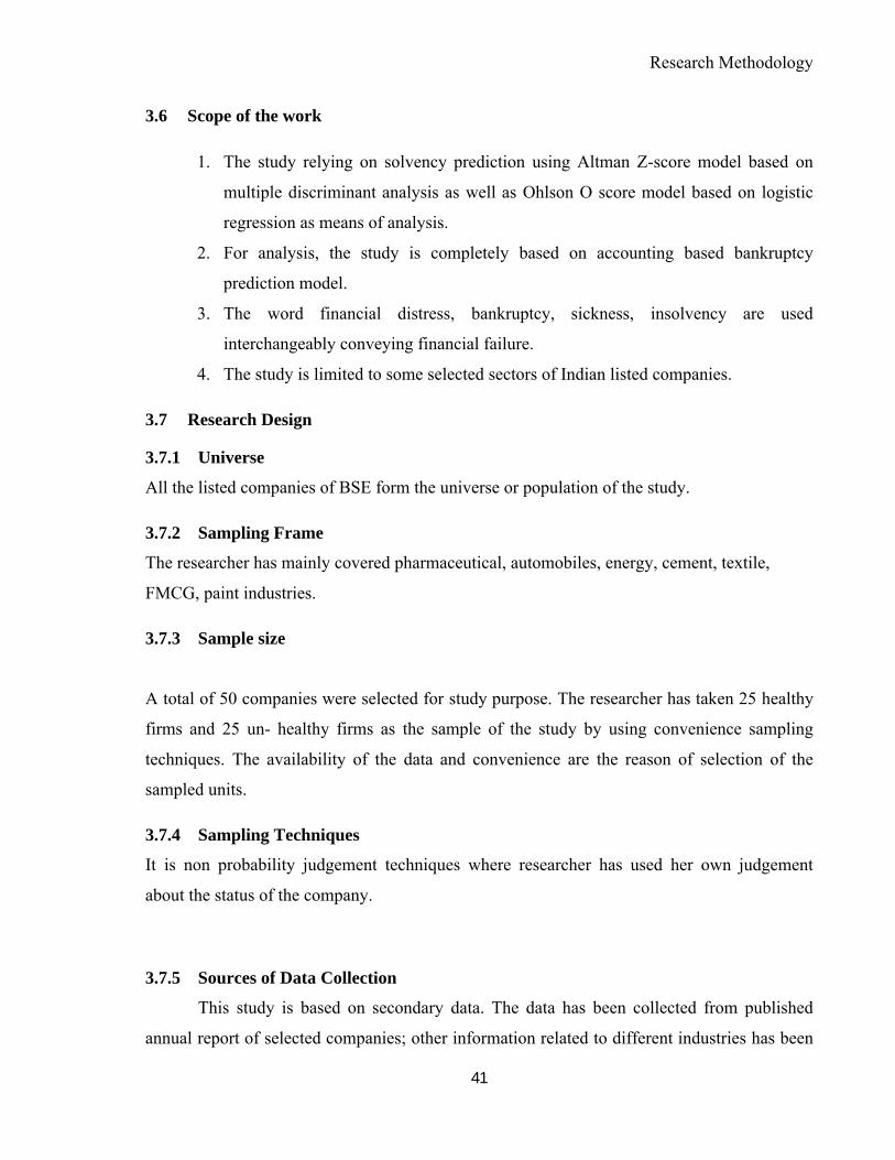
Research Methodology

41

3.6 Scope of the work

1. The study relying on solvency prediction using Altman Z-score model based on

multiple discriminant analysis as well as Ohlson O score model based on logistic

regression as means of analysis.

2. For analysis, the study is completely based on accounting based bankruptcy

prediction model.

3. The word financial distress, bankruptcy, sickness, insolvency are used

interchangeably conveying financial failure.

4. The study is limited to some selected sectors of Indian listed companies.

3.7 Research Design

3.7.1 Universe

All the listed companies of BSE form the universe or population of the study.

3.7.2 Sampling Frame

The researcher has mainly covered pharmaceutical, automobiles, energy, cement, textile,

FMCG, paint industries.

3.7.3 Sample size

A total of 50 companies were selected for study purpose. The researcher has taken 25 healthy

firms and 25 un- healthy firms as the sample of the study by using convenience sampling

techniques. The availability of the data and convenience are the reason of selection of the

sampled units.

3.7.4 Sampling Techniques

It is non probability judgement techniques where researcher has used her own judgement

about the status of the company.

3.7.5 Sources of Data Collection

This study is based on secondary data. The data has been collected from published

annual report of selected companies; other information related to different industries has been

Research Methodology

42

collected from official website and annual report, books and journals, news paper etc. The

references books have been referred from the library of various universities. Thus, various

sources have been used for collection of the relevant data. No primary data has been collected.

The researcher has also used some of the Ph.D thesis for obtaining conceptual background

which are already been acknowledged.

3.8 Statistical Tools& Techniques for bankruptcy prediction models

3.8.1 Multiple Discriminant Analysis:

MDA is statistical technique and it is used when independent variables are quantitative and

dependent variable is qualitative which in our case safe, grey and distress firms are. The

relationship is expressed as the ratio of between group variance to within group variance. DA

is form of linear combination, that discriminates between the predefined classes and estimate

the constant and product terms to minimize the within group sum of squares to measure the

variation. When the covariance matrices for every group are equal, and the variable follows a

multivariate normal distribution, Discriminant analysis performs better. Though, empirical

studies have proved that the problems connected with normality assumptions weaken DA’s

prediction ability, but not its classification capability.

More the eigen value more is the accuracy of model. Depending about the eigen value,

discriminant coefficient are chosen to maximize the eigen value. For obtaining discriminant

function, key assumptions are multivariate normality of the independent variables and

unknown dispersion and covariance matrices for the group.

3.8.2 Logistic Regression:

For prediction of bankruptcy Ohlson (2008) used logistic regression named as logit model for

the first time and then after followed by others. Logistic regression analysis helps in predicting

probability of occurrence of dependent variable given the value of independent variable, when

dependent variable is dichotomous. Independent variables can be continuous or categorical.

Logistic regression is a more flexible technique because it makes no assumptions about nature

of relationship between independent and dependent variables. Moreover, independent

variables are not required to be normally distributed. When dependent variable is

dichotomous, we cannot directly apply linear regression. One of the assumptions of linear

Research Methodology

43

regression is that the relationship between variables is linear. When dependent variable is

dichotomous, this assumption is violated. Logistic regression overcomes the problem of

violating the assumption of linearity.

In logistic regression the dependent variable is the probability that an event will occur, hence y

is constrained between 0 and 1. The predictors can be binary, a mixture of categorical and

continuous or just continuous. The logistic equation can be rearranged into linear form by

converting the probability into a log odds or logit

Table 4: Logistic Regression – Description of Terms

Sr. no. Term Description

1

Omnibus Test of

Model

coefficient

How well the model performs. Chi-square must decreases from

step 1 to next step with p value <0.05 in each step in Backward

Stepwise and increases in Forward Stepwise.

2-2 Log

likelihood

Used to compare models and assess of the inclusion of additional

terms in the model significantly improves models fit or not.

The value of -2LL must be decreases from step 1 to next in each

step in Backward Stepwise and increases in Forward Stepwise.

3

Cox & Snell and

Nagelkerke R

Square

Give an appropriation about how much variance in the dependent

variable can be explained by independent variables.

The value of Cox & Snell and Nagelkerke R Sqaure must be

decreases from step 1 to next in each step in Backward Stepwise

and increases in Forward Stepwise.

4

Hosmer and

Lemeshow Test

This test generates chi-square statistics and check validity of

overall model.

The value of Hosmer and Lemeshow Test increases from step 1

to next in each step in Backward Stepwise and decreases in

Forward Stepwise.

5 Classification

Table

It measuring how well group is predicted accurate classification

Research Methodology

44

3.9 Limitations of the study

The main limitation of the study as under:

1. The studies is restricted to only limited units as compare to population, whose

authentic financial data was available.

2. The present study limits itself to the Altman model of Z – score and Ohlson- O score model.

Data Analysis & Interpretation

45

CHAPTER 4

Data Analysis and Interpretation

4 Data Analysis and Interpretation

4.1 Edward Altman Model

Businesses are enterprises which produce goods or render services for profit motive. To be

able to predict the financial soundness of a business has led to many research works. Financial

ratios are a key indicator of financial soundness of a business. Financial ratios are a tool to

determine the operational & financial efficiency of business undertakings. There exist a large

number of ratios propounded by various authors. Altman (1968) developed a new model

called Z-score model using ratios as its base for predicting liquidity position. The Z score is

multivariate formula. The model covers both the problems, financial and operating problems13.

With the help of the Z- Score model, Altman could predict financial efficiency/Bankruptcy up

to 2-3 years in advance. Altman made regular changes to achieve the perfect equation which

could predict bankruptcy. It can be safely said that Altman‘s Z-score Model can be applied to

modern economy to predict distress and bankruptcy one, two & three years in advance.

For study Altman stratified and matched 33 bankrupt manufacturing with 33 non bankrupt

manufacturing firms as sample. The discriminant function with variables and coefficient

constructed are as follow:

Z =.1.2X1 + 1.4X2 + 3.3X3 + 0.6X4 + 0.9X5

13The model uses five ratios symbolically X1, X2, X3 X4 and X5.The ratio X1, X2 and X4 for financial problems and X3 and X5 for operating problems.

Data Analysis & Interpretation

46

Table 5: Description of the ratio used by Altman

Financial Ratios

Descriptions

X1 Working Capital/Total Assets(Stand for liquidity measure)

X2 Retained Earnings/Total Assets(Stand for measure of reinvested earning )

X3Earnings before interest and tax/Total Assets (Stand for profitability measure)

X4 Market value of equity shares/Total liability (Stand for leverage measure)

X5 Net sales/Total Assets (Stand for sales generating ability)

The Z-score is composite credit score for manufactures involving measures of firm‘s

performance including measures of corporate liquidity, cumulative and current profitability,

leverage and sales productivity. Each measure is assigned a compute determined weighting

such, that when an analyst multiplies the weights lines the financial performance and sums up

of this five factors, the result is the overall Z-score.

Zones Z

Safe Zones Z > 2.99

Grey Zones 1.81<Z<2.99

Distress Zones Z<1.81

4.1.1 Result based on Altman Z score ModelUsing Altman formula, result of status of the companies are obtained below

Data Analysis & Interpretation

47

Table 6: Results Based on Altman Z Score Model

Sr. No. Name of the company A B C D E Z score Remarks1 Hindustan chemical Organic 0.060830 -0.588330 -0.131310 0.534978 1.028803 0.165792 Distress2 Winsome Diamond -0.808740 0.021052 0.008302 0.014109 1.410941 0.505793 Distress3 Surya Pharma 0.124138 0.155535 0.075921 0.000000 0.521422 1.138676 Distress4 Ambuja Cement 0.234609 0.705871 0.089253 2.202838 0.661513 3.547501 Safe5 Murli Industries 0.037783 0.186477 0.053053 0.251325 0.353981 0.986258 Distress6 Deccan Chronicals 0.478818 0.513653 0.000000 0.000000 0.364429 1.658125 Distress7 Electrotherm -0.176290 0.190725 0.063064 0.062051 0.620509 0.921321 Distress8 Kemrock 0.101623 0.161519 0.000000 0.658889 0.470626 1.214032 Distress9 KS oil 0.114584 0.360574 0.139809 0.479999 1.307229 2.698901 Gray

10 Varun Industry 0.049345 0.094866 0.069132 0.242773 1.348745 1.91457107 Gray11 Sterling biotech -0.47946 0.195077 0.03054 0.031056 0.097052 -0.0857749 Distress12 S kumar nationwide 0.416138 0.107024 0 0 0.625637 1.27483692 Distress13 Orchid pharma 0.050195 0.244669 -0.08505 0.290633 0.330263 0.62674069 Distress14 Alps industries Ltd 0.120001 -0.12626 0.008721 0.010528 0.526327 0.52866663 Distress15 European Projects and Aviation Ltd -0.39035 0.003071 0.014235 0.033927 0.339271 -0.0575224 Distress16 Housing development and Infra Ltd. 0.608279 0.598609 0.598609 0.11747 0.059328 3.67320834 Safe17 ACC Ltd -0.03412 0.642879 0.078224 1.932049 0.890345 3.1668013 Safe18 pradip oversea 0.173813 0.221943 0.151397 0 1.382413 2.40131795 Gray19 Berger Paints India 0.580348 0.529224 0.186547 6.237938 1.641563 7.43726203 Safe20 shah alloys -0.08097 -0.06319 -0.02141 0.217207 0.775737 0.64976449 Distress21 shiv vani oil -0.00686 0.212481 0.09396 0.039595 0.232914 0.855977 Distress22 Sujana 0.247734 0.226742 0.048297 0 1.729538 2.50363822 Gray23 Lypsa Gems 0.151258 0.05615 0.053614 0.837427 2.701379 3.64088331 Safe24 Asian Paints 0.194062 0.568435 0.271439 10.51732 1.579177 9.81399948 Safe25 Bajaj Auto 0.324468 0.668459 0.284763 3.661447 1.356092 5.81788223 Safe26 Captain Polyplast 0.174981 0.154469 0.120917 0.507701 1.103697 2.23357711 Gray27 Cipla 0.196153 0.719437 0.110324 3.594945 0.637402 4.40103292 Safe28 Coal India 0.3837 0.470333 0.627384 10.19737 0.017246 9.32494414 Safe29 Dr. Reddy 0.347879 0.641031 0.129048 3.583438 0.603272 4.49409249 Safe30 Gail 0.011402 0.526552 0.086642 0.930467 1.069503 2.66455873 Gray31 Goenka Diamond and Jewels 0.385122 0.375547 0.025627 0.063844 0.141875 1.25266107 Distress32 Hero Motocorp 0.132936 0.617903 0.332166 4.964835 2.599447 7.69908218 Safe

Data Analysis & Interpretation

48

33 HUL 0.035259 0.257279 0.406331 13.56494 2.212877 12.0952338 Safe34 Nestle India Ltd 0.165099 0.447568 0.237456 9.178066 1.335963 8.45112129 Safe35 ITC 0.2777 0.676124 0.318016 5.837563 0.816442 6.64824664 Safe36 Larsen and Tourbo 0.206243 0.424413 0.08933 1.837075 0.656098 2.89480217 Gray37 Lupin 0.435343 0.811962 0.292258 8.076771 0.873164 8.34283598 Safe38 Mahindra and Mahindra 0.035026 0.575161 0.122856 2.097592 1.165329 3.6765654 Safe39 Maruti Suzuki -0.01863 0.702012 0.151239 3.245101 1.448706 4.8553143 Safe40 NTPC 0.034726 0.372489 0.067434 0.611811 0.368561 1.52133651 Distress41 ONGC 0.052815 0.674372 0.127634 1.251156 0.394686 2.57406988 Gray42 Aurobindo Pharma 0.236839 0.52126 0.200236 3.449992 0.784089 4.5288338 Safe43 Reliance Industries 0.062473 0.535272 0.080031 0.67009 0.827271 2.31777426 Gray44 Sun pharmaceutical industries -0.1496 0.601694 -0.02691 5.452553 0.206458 4.05203526 Safe45 Tata Motors -0.23622 0.284242 -0.03923 3.50685 0.718627 2.80774903 Gray46 Tata Steels -0.04128 0.567895 0.074293 0.265057 0.358185 1.50790868 Distress47 Himatsingka Seide -0.07823 0.463563 0.112644 0.560084 0.666766 1.92965671 Gray48 HMT Watches 0.117565 -0.44301 0.000856 2.073201 0.106264 0.87387061 Distress49 Bhushan steel 0.013331 0.205786 0.057821 0.22393 0.238224 0.86748972 Distress50 Hindustan fluorocarbon 0.133948 -1.91771 0.212546 1.459694 0.705166 -0.2416745 Distress

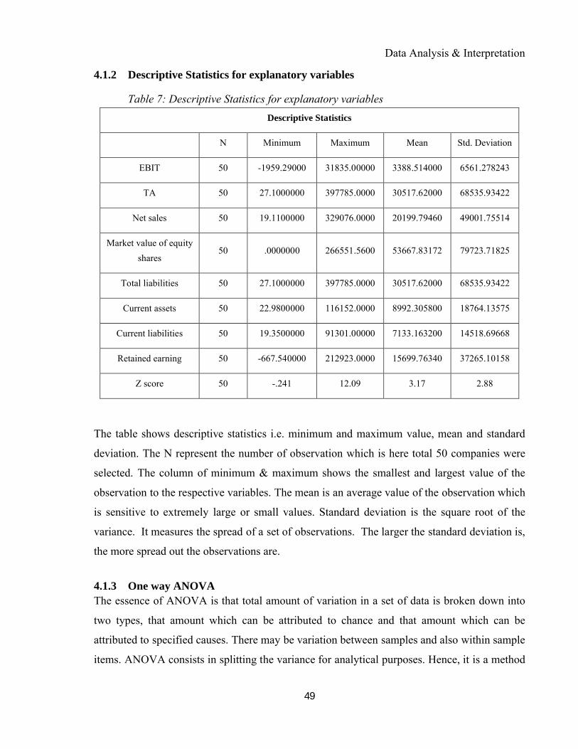
Data Analysis & Interpretation

49

4.1.2 Descriptive Statistics for explanatory variables

Table 7: Descriptive Statistics for explanatory variables

Descriptive Statistics

N Minimum Maximum Mean Std. Deviation

EBIT 50 -1959.29000 31835.00000 3388.514000 6561.278243

TA 50 27.1000000 397785.0000 30517.62000 68535.93422

Net sales 50 19.1100000 329076.0000 20199.79460 49001.75514

Market value of equity

shares50 .0000000 266551.5600 53667.83172 79723.71825

Total liabilities 50 27.1000000 397785.0000 30517.62000 68535.93422

Current assets 50 22.9800000 116152.0000 8992.305800 18764.13575

Current liabilities 50 19.3500000 91301.00000 7133.163200 14518.69668

Retained earning 50 -667.540000 212923.0000 15699.76340 37265.10158

Z score 50 -.241 12.09 3.17 2.88

The table shows descriptive statistics i.e. minimum and maximum value, mean and standard

deviation. The N represent the number of observation which is here total 50 companies were

selected. The column of minimum & maximum shows the smallest and largest value of the

observation to the respective variables. The mean is an average value of the observation which

is sensitive to extremely large or small values. Standard deviation is the square root of the

variance. It measures the spread of a set of observations. The larger the standard deviation is,

the more spread out the observations are.

4.1.3 One way ANOVAThe essence of ANOVA is that total amount of variation in a set of data is broken down into

two types, that amount which can be attributed to chance and that amount which can be

attributed to specified causes. There may be variation between samples and also within sample

items. ANOVA consists in splitting the variance for analytical purposes. Hence, it is a method

Data Analysis & Interpretation

50

of analyzing the variance to which a response is subject into its various components

corresponding to various source of variation.

Thus in general through ANOVA technique one can, investigate any number of factors which

are hypothesizes or said to influence the dependent variable. One may as well investigate the

differences amongst various categories within each of these factors which may have a large

number of possible values. If we take only one factor and investigate the differences amongst

its various categories having numerous possible values, we are said to use one-way ANOVA

and in case we investigate two factors at the same time, then we use two-way ANOVA.

Dependent variable: Status of company (Safe, Grey, financial distress)

Independent variable: Working Capital to Total Assets

H0: There is no significant difference on working capital to total assets between all

selected units under different status of company.

H1: There is at least one significant difference on working capital to total assets between

all selected units under different status of company.

4.1.3.1 Descriptive StatisticTable 8: Descriptive Statistic

Descriptives

Working Capital to Total Assets

N Mean Std. Deviation Std. Error95% Confidence Interval for Mean

Lower Bound Upper Bound

Safe 19 .217716380 .2010811487 .0461311793 .120798369 .314634391

Grey 11 .070812895 .1392430144 .0419833485 -.022731835 .164357625

Distress 20 .004513832 .2997346685 .0670227094 -.135766311 .144793975

Total 50 .100116594 .2508628400 .0354773631 .028822164 .171411024

Data Analysis & Interpretation

51

The Descriptive table provides some very useful descriptive statistics, including the mean,

standard deviation and 95% confidence intervals for the dependent variable (Working capital

to Total Assets) for each separate group (Safe, Grey and Distress), as well as when all groups

are combined (Total). These figures are useful when you need to describe your data.

4.1.3.2 Test of Homogeneity of VariancesTable 9: Test of Homogeneity of Variances

Working Capital to Total Assets

Levene Statistic df1 df2 Sig.

1.346 2 47 .270

Levene’s Test checks whether the population variances of Working capital to Total Assets are

equal for all the three statuses are, which is a one of the requirement for ANOVA. Here p

value is 0.270 which is greater than 0.05 so null hypothesis cannot be rejected and it is

concluded that population variances are equal. We satisfy this assumption for our ANOVA.

4.1.3.3 Result of ANOVA

Table 10: Result of ANOVA

ANOVA

Working Capital to Total Assets

Sum of Squares Df Mean Square F Sig.

Between Groups .455 2 .228 4.068 .023

Within Groups 2.629 47 .056

Total 3.084 49

The above table shows the output of the ANOVA analysis and states whether there is a

statistically significant difference between our group means or not. We can see that the

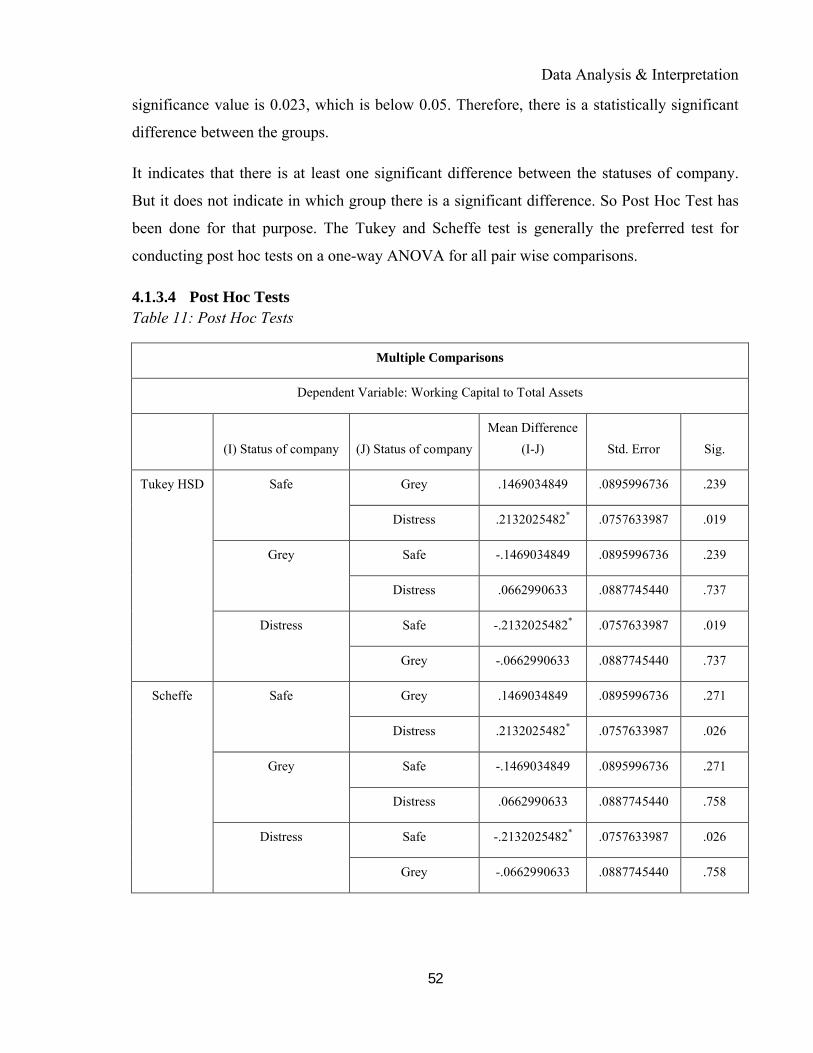
Data Analysis & Interpretation

52

significance value is 0.023, which is below 0.05. Therefore, there is a statistically significant

difference between the groups.

It indicates that there is at least one significant difference between the statuses of company.

But it does not indicate in which group there is a significant difference. So Post Hoc Test has

been done for that purpose. The Tukey and Scheffe test is generally the preferred test for

conducting post hoc tests on a one-way ANOVA for all pair wise comparisons.

4.1.3.4 Post Hoc TestsTable 11: Post Hoc Tests

Multiple Comparisons

Dependent Variable: Working Capital to Total Assets

(I) Status of company (J) Status of company

Mean Difference

(I-J) Std. Error Sig.

Tukey HSD Safe Grey .1469034849 .0895996736 .239

Distress .2132025482* .0757633987 .019

Grey Safe -.1469034849 .0895996736 .239

Distress .0662990633 .0887745440 .737

Distress Safe -.2132025482* .0757633987 .019

Grey -.0662990633 .0887745440 .737

Scheffe Safe Grey .1469034849 .0895996736 .271

Distress .2132025482* .0757633987 .026

Grey Safe -.1469034849 .0895996736 .271

Distress .0662990633 .0887745440 .758

Distress Safe -.2132025482* .0757633987 .026

Grey -.0662990633 .0887745440 .758

Data Analysis & Interpretation

53

From above table, it is concluded that based on both the methods there is a significant

difference between the Safe and Distress Company and there is no significant difference

between Safe and Grey Company and also there is no significant difference between Grey and

Distress Company.

Independent variable: Retained Earnings to Total Assets

Dependent variable: Status of company (Safe, Grey, financial distress)

H0: There is no significant difference on Retained Earnings to total assets between all

selected units under different status of company.

H1: There is at least one significant difference on Retained Earnings to total assets

between all selected units under different status of company.

4.1.3.5 Descriptive statisticTable 12: Descriptive statistic

Descriptives

Retained Earnings to Total Assets

N Mean Std. Deviation Std. Error

95% Confidence Interval for Mean

Lower Bound Upper Bound

Safe 19 .569020544 .1736862082 .0398463489 .485306471 .652734616

Grey 11 .360637168 .1809019510 .0545439905 .239105584 .482168753

Distress 20 .018724756 .5339926078 .1194043771 -.231191477 .268640990

Total 50 .303057886 .4353144675 .0615627624 .179342883 .426772889

The Descriptive table provides some very useful descriptive statistics, including the mean,

standard deviation and 95% confidence intervals for the dependent variable (Retained

Earnings to Total Assets) for each separate group (Safe, Grey and Distress), as well as when

all groups are combined (Total). These figures are useful when you need to describe your data.

Data Analysis & Interpretation

54

4.1.3.6 Test of Homogeneity of VariancesTable 13 : Test of Homogeneity of Variances

Retained Earnings to Total Assets

Levene Statistic df1 df2 Sig.

2.953 2 47 .062

Levene’s Test checks whether the population variances of Working capital to Total Assets for

the three statuses are all equal, which is a requirement for ANOVA. Here p value is 0.62

which is greater than 0.05 so null hypothesis cannot be rejected and it conclude that population

variances are equal. We satisfy this assumption for our ANOVA.

4.1.3.7 Result of ANOVATable 14: Result of ANOVA

ANOVA

Retained Earnings to Total Assets

Sum of Squares Df Mean Square F Sig.

Between Groups 2.997 2 1.499 11.202 .000

Within Groups 6.288 47 .134

Total 9.285 49

This is the table that shows the output of the ANOVA analysis and whether there is a

statistically significant difference between our group means. We can see that the significance

value is 0.000, which is below 0.05. Therefore, there is a statistically significant difference

between the groups.

It indicates that there is at least one significant difference between the statuses of company.

But it does not indicate in which group there is a significant difference. So Post Hoc Test has

Data Analysis & Interpretation

55

been done for that purpose. The Tukey and Scheffe test is generally the preferred test for

conducting post hoc tests on a one-way ANOVA for all pair wise comparisons.

4.1.3.8 Post Hoc TestsTable 15: Post Hoc Tests

Multiple Comparisons

Dependent Variable: Retained Earnings to Total Assets

(I) Status of company (J) Status of company

Mean Difference

(I-J) Std. Error Sig.

Tukey HSD Safe Grey .2083833754 .1385789781 .298

Distress .5502957874* .1171791586 .000

Grey Safe -.2083833754 .1385789781 .298

Distress .3419124120* .1373027946 .042

Distress Safe -.5502957874* .1171791586 .000

Grey -.3419124120* .1373027946 .042

Scheffe Safe Grey .2083833754 .1385789781 .331

Distress .5502957874* .1171791586 .000

Grey Safe -.2083833754 .1385789781 .331

Distress .3419124120 .1373027946 .054

Distress Safe -.5502957874* .1171791586 .000

Grey -.3419124120 .1373027946 .054

From above table, it conclude that that based on both method there is a significant difference

between the Safe and Distress company and there is a significant difference between Grey and

Distress company and there is no significant difference between Grey and Distress company.

Independent variable: Earnings before Interest & Tax to Total Assets

Dependent variable: Status of company (Safe, Grey, financial distress)

Data Analysis & Interpretation

56

H0: There is no significant difference on Earnings before Interest & Taxto total assets

between all selected units under different status of company.

H1: There is at least one significant difference on Earnings before Interest & Taxto total

assets between all selected units under different status of company.

4.1.3.9 Descriptive StatisticTable 16: Descriptive Statistic

Descriptives

Earnings before Interest & Tax to Total Assets

N Mean Std. Deviation Std. Error

95% Confidence Interval for Mean

Lower Bound Upper Bound

Safe 19 .234886957 .1725929900 .0395955475 .151699799 .318074115

Grey 11 .089690998 .0530288097 .0159887877 .054065759 .125316237

Distress 20 .027429787 .0695077686 .0155424096 -.005100850 .059960424

Total 50 .119960978 .1490361540 .0210768950 .077605372 .162316584

The Descriptive table provides some very useful descriptive statistics, including the mean,

standard deviation and 95% confidence intervals for the dependent variable (Earnings before

Interest & Tax to Total Assets) for each separate group (Safe, Grey and Distress), as well as

when all groups are combined (Total). These figures are useful when you need to describe

your data.

4.1.3.10 Test of Homogeneity of VariancesTable 17: Test of Homogeneity of Variances

Earnings before Interest & Tax to Total Assets

Levene Statistic df1 df2 Sig.

8.185 2 47 .001

Data Analysis & Interpretation

57

Levene’s Test checks whether the population variances of Working capital to Total Assets for

the three statuses are all equal, which is a requirement for ANOVA. Here p value is 0.001

which is less than 0.05 so null hypothesis can be rejected and it conclude that population

variances are not equal. As ANOVA is robust test and it tolerate minor violation of the

assumption so we can go for ANOVA.

4.1.3.11 Robust Tests of Equality of MeansTable 18: Robust Tests of Equality of Means

Earnings before Interest & Tax to Total Assets

Statistica df1 df2 Sig.

Welch 12.881 2 28.873 .000

a. Asymptotically F distributed.

This is the table that shows the output of the ANOVA analysis and whether there is a

statistically significant difference between our group means. Here we used Welch statistics

because of not homogeneous variance. We can see that the significance value is 0.000, which

is below 0.05. Therefore, there is a statistically significant difference between the groups.

It indicates that there is at least one significant difference between the statuses of company.

But it does not indicate in which group there is a significant difference. So Post Hoc Test has

been done for that purpose. The Games Howell test is generally the preferred test for

conducting post hoc tests on a one-way ANOVA for all pair wise comparisons when

population variances are unequal.

Data Analysis & Interpretation

58

4.1.3.12 Post Hoc TestsTable 19: Post Hoc Tests

Multiple Comparisons

Earnings before Interest & Tax to Total Assets

Games-Howell

(I) Status of company (J) Status of company

Mean Difference

(I-J) Std. Error Sig.

Safe Grey .1451959589* .0427018584 .007

Distress .2074571700* .0425367356 .000

Grey Safe -.1451959589* .0427018584 .007

Distress .0622612111* .0222981575 .025

Distress Safe -.2074571700* .0425367356 .000

Grey -.0622612111* .0222981575 .025

From above table, it conclude that that based on both method there is a significant difference

between all status i.e. between Safe and Grey Company; Safe and Distress Company and Grey

and Distress Company

Independent variable: Market value of Equity Shares to Total Liabilities

Dependent variable: Status of company (Safe, Grey, financial distress)

H0: There is no significant difference on Market value of Equity Shares to Total Liabilities

between all selected units under different status of company.

H1: There is at least one significant difference on Market value of Equity Shares to Total

Liabilities between all selected units under different status of company.

Data Analysis & Interpretation

59

4.1.3.13 Descriptive StatisticTable 20: Descriptive Statistic

Descriptives

Market value of Equity Shares to Total Liabilities

N Mean Std. Deviation Std. Error

95% Confidence Interval for

Mean

Lower Bound Upper Bound

Safe 19 5.197350203 3.6325359280 .8333608957 3.446523930 6.948176476

Grey 11 .907835807 1.0172506283 .3067126047 .224437536 1.591234078

Distress 20 .342091797 .5385219741 .1204171741 .090055755 .594127839

Total 50 2.311553673 3.2288643553 .4566303762 1.393920577 3.229186770

The Descriptive table provides some very useful descriptive statistics, including the mean,

standard deviation and 95% confidence intervals for the dependent variable (Market value of

Equity Shares to Total Liabilities) for each separate group (Safe, Grey and Distress), as well as

when all groups are combined (Total). These figures are useful when you need to describe

your data.

4.1.3.14 Test of Homogeneity of VariancesTable 21: Test of Homogeneity of Variances

Market value of Equity Shares to Total Liabilities

Levene Statistic df1 df2 Sig.

18.847 2 47 .000

Levene’s Test checks whether the population variances of Working capital to Total Assets for

the three statuses are all equal, which is a requirement for ANOVA. Here p value is 0.000

which is less than 0.05 so null hypothesis can be rejected and it conclude that population

variances are not equal. As ANOVA is robust test and it tolerate minor violation of the

assumption so we can go for ANOVA.

Data Analysis & Interpretation

60

4.1.3.15 Robust Tests of Equality of MeansTable 22: Robust Tests of Equality of Means

Market value of Equity Shares to Total Liabilities

Statistica df1 df2 Sig.

Welch 17.073 2 20.473 .000

a. Asymptotically F distributed.

This is the table that shows the output of the ANOVA analysis and whether there is a

statistically significant difference between our group means. Here we used Welch statistics

because of not homogeneous variance. We can see that the significance value is 0.000, which

is below 0.05. Therefore, there is a statistically significant difference between the groups.

It indicates that there is at least one significant difference between the statuses of company.

But it does not indicate in which group there is a significant difference. So Post Hoc Test has

been done for that purpose. The Games Howell test is generally the preferred test for

conducting post hoc tests on a one-way ANOVA for all pair wise comparisons when

population variances are unequal.

4.1.3.16 Post Hoc TestsTable 23: Post Hoc Tests

Multiple Comparisons

Market value of Equity Shares to Total Liabilities

Games-Howell

(I) Status of company (J) Status of company

Mean Difference

(I-J) Std. Error Sig.

Safe Grey 4.2895143963* .8880107006 .000

Distress 4.8552584059* .8420158421 .000

Data Analysis & Interpretation

61

Grey Safe -4.2895143963* .8880107006 .000

Distress .5657440096 .3295040481 .236

Distress Safe -4.8552584059* .8420158421 .000

Grey -.5657440096 .3295040481 .236

From above table, it concludes that that based on both method there is a significant difference

between all status i.e. between Safe and Grey Company; Safe and Distress Company and Grey

and Distress Company.

Independent variable: Net Sales to Total Assets

Dependent variable: Status of company (Safe, Grey, financial distress)

H0: There is no significant difference on Net Sales to Total Assets between all selected

units under different status of company.

H1: There is at least one significant difference on Net Sales to Total Assets between all

selected units under different status of company.

4.1.3.17 Descriptive StatisticTable 24: Descriptive Statistic

Descriptives

Net Sales to Total Assets

N Mean Std. Deviation Std. Error

95% Confidence Interval for Mean

Lower Bound Upper Bound

Safe 19 1.136304817 .7738298290 .1775287381 .763330778 1.509278856

Grey 11 1.018597648 .4013703615 .1210177174 .748953370 1.288241926

Distress 20 .480809273 .3219815444 .0719972621 .330117272 .631501275

Total 50 .848211022 .6219680731 .0879595684 .671449652 1.024972393

Data Analysis & Interpretation

62

The Descriptive table provides some very useful descriptive statistics, including the mean,

standard deviation and 95% confidence intervals for the dependent variable (Net Sales to Total

Assets) for each separate group (Safe, Grey and Distress), as well as when all groups are

combined (Total). These figures are useful when you need to describe your data.

4.1.3.18 Test of Homogeneity of VariancesTable 25: Test of Homogeneity of Variances

Net Sales to Total Assets

Levene Statistic df1 df2 Sig.

6.882 2 47 .002

Levene’s Test checks whether the population variances of Working capital to Total Assets for

the three statuses are all equal, which is a requirement for ANOVA. Here p value is 0.002

which is less than 0.05 so null hypothesis can be rejected and it conclude that population

variances are not equal. As ANOVA is robust test and it tolerate minor violation of the

assumption so we can go for ANOVA.

4.1.3.19 Robust Tests of Equality of MeansTable 26: Robust Tests of Equality of Means

Net Sales to Total Assets

Statistica df1 df2 Sig.

Welch 10.750 2 24.438 .000

a. Asymptotically F distributed.

This is the table that shows the output of the ANOVA analysis and whether there is a

statistically significant difference between our group means. Here we used Welch statistics

Data Analysis & Interpretation

63

because of not homogeneous variance. We can see that the significance value is 0.000, which

is below 0.05. Therefore, there is a statistically significant difference between the groups.

It indicates that there is at least one significant difference between the statuses of company.

But it does not indicate in which group there is a significant difference. So Post Hoc Test has

been done for that purpose. The Games Howell test is generally the preferred test for

conducting post hoc tests on a one-way ANOVA for all pair wise comparisons when

population variances are unequal.

4.1.3.20 Post Hoc TestsTable 27: Post Hoc Tests

Multiple Comparisons

Net Sales to Total Assets

Games-Howell

(I) Status of company (J) Status of company

Mean Difference

(I-J) Std. Error Sig.

Safe Grey .1177071693 .2148528352 .848

Distress .6554955438* .1915725936 .006

Grey Safe -.1177071693 .2148528352 .848

Distress .5377883745* .1408151045 .004

Distress Safe -.6554955438* .1915725936 .006

Grey -.5377883745* .1408151045 .004

From above table, it concludes that based on both method there is a significant difference

between the Safe and Distress Company and Grey and Distress Company and there is no

significant difference between Safe and Grey Company.

4.1.4 Discriminant AnalysisDiscriminant Analysis (DA) is a technique for analyzing data when the criterion or dependent

variable is categorical and the predictor or independent variables are interval in nature.

Data Analysis & Interpretation

64

In the estimation part of research we firstly decided to use the DA procedure. Discriminant

Analysis is used primarily to predict membership in two or more mutually exclusive groups.

Present study also used various ratios for financial analysis which has used in Edward Altman

model. The following ratios have been used in study:

Dependent variable: Status of the company (Safe, Grey, Distress)

Independent variable:

4.1.4.1 Descriptions of the variables

Table 28: Descriptions

Financial

RatiosDescriptions

X1 Working Capital/Total Assets(Stand for liquidity measure)

X2 Retained Earnings/Total Assets(Stand for measure of reinvested earning )

X3 Earnings before interest and tax/Total Assets (Stand for profitability measure)

X4 Market value of equity shares/Total liability (Stand for leverage measure)

X5 Net sales/Total Assets (Stand for sales generating ability)

4.1.4.2 Group StatisticsTable 29: Group Statistics

Status of company Mean Std. DeviationValid N (listwise)

Unweighted Weighted

Safe

X1 .217716380 .2010811487 19 19.000

X2 .569020544 .1736862082 19 19.000

X3 .234886957 .1725929900 19 19.000

X4 5.197350203 3.6325359280 19 19.000

Data Analysis & Interpretation

65

X5 1.136304817 .7738298290 19 19.000

Grey

X1 .070812895 .1392430144 11 11.000

X2 .360637168 .1809019510 11 11.000

X3 .089690998 .0530288097 11 11.000

X4 .907835807 1.0172506283 11 11.000

X5 1.018597648 .4013703615 11 11.000

Distress

X1 .004513832 .2997346685 20 20.000

X2 .018724756 .5339926078 20 20.000

X3 .027429787 .0695077686 20 20.000

X4 .342091797 .5385219741 20 20.000

X5 .480809273 .3219815444 20 20.000

Total

X1 .100116594 .2508628400 50 50.000

X2 .303057886 .4353144675 50 50.000

X3 .119960978 .1490361540 50 50.000

X4 2.311553673 3.2288643553 50 50.000

X5 .848211022 .6219680731 50 50.000

This table displays the sample means and sample standard deviations for each of the variable.

4.1.4.3 Tests of Equality of Group MeansTable 30: Tests of Equality of Group Means

Wilks' Lambda F df1 df2 Sig.

X1 .852 4.068 2 47 .023

X2 .677 11.202 2 47 .000

X3 .603 15.483 2 47 .000

Data Analysis & Interpretation

66

X4 .496 23.881 2 47 .000

X5 .758 7.522 2 47 .001

An important step in DA analysis is a test of group means equality, which revealed that all

variable had significant differences between Safe, Grey and financially Distress Company.

Indiscriminant analysis we are trying to predict a group membership, so firstly we examine

whether there are any significant differences between groups on each of the independent

variables using group means and ANOVA results data. The Group Statistics and Tests of

Equality of Group Means tables provide this information. If there are no significant group

differences, it is not worthwhile proceeding any further with the analysis. A rough idea of

variables that may be important can be obtained by inspecting the group means and standard

deviations. Wilks’ lambda is significant by the F test for all independent variables.

4.1.4.4 Pooled Within-Groups MatricesTable 31 : Pooled Within-Groups Matrices

X1 X2 X3 X4 X5

Correlation

X1 1.000 .003 .294 -.029 -.172

X2 .003 1.000 -.111 -.131 -.302

X3 .294 -.111 1.000 .325 -.144

X4 -.029 -.131 .325 1.000 .079

X5 -.172 -.302 -.144 .079 1.000

This table shows the pooled within-group estimates of the covariance and correlation matrices.

It indicates the interrelationship among the variables.

Data Analysis & Interpretation

67

4.1.4.5 Log DeterminantsTable 32: Log Determinants

Status of company RankLog

Determinant

Safe 5 -9.263

Grey 5 -18.206

Distress 5 -13.783

Pooled within-groups 5 -9.070

The larger the log determinant in the table, the more that group's covariance matrix differs.

The "Rank" column indicates the number of independent variables in this case. Since

discriminant analysis assumes homogeneity of covariance matrices between groups, we would

like to see the determinants be relatively equal.

4.1.4.6 Box M Test ResultsTable 33: Box M Test Results

Box's M 184.389

F

Approx. 5.077

df1 30

df2 3837.471

Sig. .000

One of the assumptions of DA is that the variance-co-variance matrices are equivalent. Box’s

M Tests the null hypothesis that the covariance matrices do not differ between groups formed

by the dependent. Box M test with significance less than 5% revealed that groups did not have

equal covariance matrices, indicating that assumption is violated.

Data Analysis & Interpretation

68

4.1.4.7 Summary of Canonical Discriminant Functions

Table 34: Summary of Canonical Discriminant Functions

Eigenvalues

Function Eigenvalue % of Variance Cumulative %Canonical

Correlation

1 2.833a 94.8 94.8 .860

2 .156a 5.2 100.0 .367

The above table provides information on each of the discriminate functions (equations)

produced. The maximum number of discriminant functions produced is the number of groups

minus 1.The larger the eigen value, the more of the variance in the dependent variable is

explained by that function.

We are only using three groups here, namely ‘Safe’ ,’Grey’ and ‘Distress’, so two function is

displayed. 94.8% was explained by the first function and 5.2% by the second one. The

canonical correlation is the multiple correlations between the predictors and the discriminant

function. The square of canonical correlation coefficient is the percentage of variance

explained in the dependent variable.

4.1.4.8 Test of Equality of Variance

Table 35: Test of Equality of Variance

Wilks' Lambda

Test of Function(s) Wilks' Lambda Chi-square Df Sig.

1 through 2 .226 66.982 10 .000

2 .865 6.513 4 .164

Data Analysis & Interpretation

69

Wilks’ lambda indicates the significance of the discriminant function. Wilks' lambda is a

measure of how well each function separates cases into groups. Smaller values of Wilks'

lambda indicate greater discriminatory ability of the function. There is 86.5% unexplained

variance in second function but when add the first function to the predictive equation; it

reduce the unexplained variance to only about 23% (0.226). The second function isn’t

significant but the combination of the two is significant.

4.1.4.9 Standardized Canonical Discriminant Function Coefficients

Table 36: Standardized Canonical Discriminant Function Coefficients

Function

1 2

X1 .238 -.076

X2 .690 .424

X3 .410 .162

X4 .491 -.781

X5 .585 .691

The interpretation of the discriminant coefficients (or weights) is like that in multiple

Regressions. This table provides an index of the importance of each predictor like the

standardized regression coefficients (beta) did in multiple regression. They indicate the

relative importance of the independent variables in predicting the dependent. The sign

indicates the direction of the relationship. This coefficient can be used to classify new cases if

the five discriminating variables are expressed in standard score.

Data Analysis & Interpretation

70

4.1.4.10 Structure MatrixTable 37 : Structure Matrix

Function

1 2

X3 .478* -.261

X2 .404* .299

X1 .245* -.123

X4 .574 -.726*

X5 .316 .491*

It provides another way of indicating the relative importance of the predictors and it can be

seen below that the same pattern holds. Many researchers use the structure matrix correlations

because they are considered more accurate than the Standardized Canonical Discriminant

Function Coefficients. The structure matrix table shows the correlations of each variable with

each discriminate function. These Pearson coefficients are structure coefficients or

discriminant loadings. They serve like factor loadings in factor analysis. By identifying the

largest loadings for each discriminate function the researcher gains insight into how to name

each function. Generally, just like factor loadings, 0.30 is seen as the cut-off between

important and less important variables.

4.1.4.11 Canonical Discriminant Function CoefficientsTable 38 : Canonical Discriminant Function Coefficients

Unstandardized

coefficient

1 2

X1 1.007 -.322

Data Analysis & Interpretation

71

X2 1.885 1.159

X3 3.467 1.369

X4 .212 -.336

X5 1.058 1.250

(Constant) -2.475 -.767

DA model un standardized coefficients from the table reveal that X1 and X4 has negative sign

meaning that increase of this variable reduces discriminate score and increased probability of

being bankrupted. Contrary to such finding, X2, X3 and X5have positive sign, meaning that

increase of these variables causes increase of discriminate score and decreases probability of

being bankrupted. Here we can see that discrimination among Safe, Grey and Distress firms

can be done by financial ratios. This table contains the un standardized discriminant function

coefficients. These would be used like un standardized b (regression) coefficients in multiple

regressions - that is, they are used to construct the actual prediction equation which can be

used to classify new cases.

4.2 Discriminant Function:

The model should be like this:

Di=-2.475+1.007X1+1.885X2+3.467X3+0.212X4-1.058X5

4.2.1 Classification Results

Table 39: Classification Results

Classification Resultsa,c

Status of companyPredicted Group Membership

TotalSafe Grey Distress

Data Analysis & Interpretation

72

Original

Count

Safe 14 4 1 19

Grey 0 10 1 11

Distress 0 2 18 20

%

Safe 73.7 21.1 5.3 100.0

Grey .0 90.9 9.1 100.0

Distress .0 10.0 90.0 100.0

Cross-validatedb

Count

Safe 13 5 1 19

Grey 0 10 1 11

Distress 0 3 17 20

%

Safe 68.4 26.3 5.3 100.0

Grey .0 90.9 9.1 100.0

Distress .0 15.0 85.0 100.0

4.2.2 Analysis of Result

Table 40 : Analysis of Result

a. 84.0% of original grouped cases correctly classified.

b. Cross validation is done only for those cases in the analysis. In cross validation, each case is classified by the functions derived from all cases other than that case.

c. 80.0% of cross-validated grouped cases correctly classified.

This table is used to assess how well the discriminant function works. .After estimation phase

of research follows the classification. Here we used cross-validated procedure of classification

(i.e. jack knife classification), which is more honest than classical classification. The data from

the table reveal that DA model accuracy is 68.4% for Safe firms, 26.3% Grey firms and 5.3%

for Distress firms and 84% in total. According to the table above when the discriminant

Data Analysis & Interpretation

73

functions were used to “predict” from the five variables, 84% of the original grouped cases

were correctly reclassified back into their original categories.

4.3 Ohlson Model

Ohlson (1980) used logit regression for his bankruptcy prediction model. Like MDA, the logit

regression is suitable when dependent variable (y) is qualitative and the independent variables

(x) are quantitative. Unlike the MDA, the logit regression does assume linearity of relationship

between the independent and dependent variable. The same nine independent variables used

by Ohlson (1980) are employed.

O = - 1.32 - 0.407 log (TA/GNP) + 6.03(TL/TA)- 1.43(WC/TA) + 0.757(CL/CA)–

2.37(NI/TA) – 1.83(FFO/TL) + 0.285Y – 1.72X– 0.521

1

)1(

NINI

NINI

Where,

TA = total assets

GNP = Gross National Product price index level

TL = total liabilities

WC = working capital

CL = current liabilities

CA = current assets

X = 1 if TL > TA, 0 otherwise

NI = net income

FFO = funds from operations

Y = 1 if a net loss for the last two years, 0 otherwise

The value of dependent variable Y is the ‘o’ score. Since Ohlson has used logistic regression

to determine the coefficients of independent variables, ‘o’ score is the log odd of the company

being financially distressed.

Data Analysis & Interpretation

74

Probability of failure = ? ?? (‘? ’??? ?? )

? ? ? ?? (‘? ’??? ?? )Ohlson (1980) gave the cut off at 50%.

P(Y) > 0.50 indicates failed, P(Y) < 0.50 indicates non- failed

For the O-Score, any results larger than 0.5 suggests that the firm will default within two

years. Then we have done logistic regression based on the category of bankrupt and not

bankrupt.

4.3.1 Description of Ohlson O score Variables

Table 41: Description of Ohlson O score Variables

Data Analysis & Interpretation

75

Name of the company

TAGNPprice

TL WC CL CA NI Nit-1Net Loss

FFO X Y TA/GNP

Hindustan chemical Organic

465.23 135.2703 465.23 28.3 203.17 231.47 -83.08 -25.28 Y -57.8 0 13.439261

9

Winsome Diamond

5,057.52107.9395

25,057.52 -4090.2 4,206.88 116.68 -33.5 95.75 N -25.81 0 0

46.855127

Surya Pharma 620.89117.5908

1620.89 114.15 313.96 428.11 46.74 27.32 N 65.68 0 0

5.2800893

ambuja Cement14,161.9

3118.1575

514,161.9

33322.5 3,226.09 6,548.60 807.56

1,496.36

N1797.8

70 0

119.85632

Murli Industries 1,315.65127.5301

81,315.65 219.2 175.56 394.76 46.06 55.63 N 78.77 0 0

10.316382

Deccan Chronicals

980.1104.2246

2980.1 394.93 84.99 479.92 66.87 32.05 N 9.96 0 0

9.4037281

Electrotherm 2,848.22 135.2703 2,848.22 8.55 1,220.38 1,228.93 53.8 52.25 N 152.67 0 021.05576

7

Kemrock 122.84104.2246

2122.84 0.57 54.77 55.34 4.53 1.53 N 3.21 0 0 .178608

3

KS oil 1,365.43117.5908

11,365.43 358.75 545.45 904.2 122.7 60.85 N 197.29 0 0

11.611706

Varun Industry 2,236.26107.9395

22,236.26 986.33 850.87 1,837.20 -34.48 -158.06 Y -17.95 0 1

20.717713

Sterling biotech 7,398.83107.9395

27,398.83 -3547.4 4,980.92 1,433.49 -400.65 -346.77 Y -338.76 0 1 68.54607

S kumar nationwide

1,513.13104.2246

21,513.13 642.44 477.83 1,120.27 99.77 -19.14 N 40.92 0 0

14.517971

Orchid pharma 4,138.33127.5301

84,138.33 248.17 1,355.66 1,603.83 -52.17 184.54 N 133.55 0 0

32.449809

Data Analysis & Interpretation

76

Alps industries Ltd

1,088.37127.5301

81,088.37 175.56 310.46 486.02 11.88 30.66 N 50.37 0 0

8.5342152

European Projects and Aviation Ltd

7,241.03107.9395

27,241.03 -724.66 3,039.54 2,314.88 -519.37 158.36 N -361.76 0 0

67.084141

Housing development and Infrastructure Ltd.

16,309.07

107.93952

16,309.07

9920.46

5,360.6515,281.1

1145.38 386.97 N 172.93 0 0

151.09452

ACC Ltd12,840.8

2118.1575

512,840.8

2-438.11 3,808.76 3,370.65 591.57

1,168.29

N 498.89 0 0108.6754

1

pradip oversea 1,438.15 100 1,438.15 518.94 711.21 1,230.15 -76.65 68.53 N -107.61 0 0 14.3815

Berger Paints India

2,310.25118.1575

52,310.25 463.53 969.5 1,433.03 266.03 234.25 N 474.87 0 0

19.552284

shah alloys 947.65127.5301

8947.65 111.13 275.81 386.94 -103.99 -120.45 Y -143.35 0 1

7.4307901

shiv vani oil 4,107.85107.9395

24,107.85 -48.1 1,365.02 1,316.92 68.7 42.09 N 216.75 0 0 38.05696

Sujana 1,942.16118.1575

51,942.16 481.14 1,081.83 1,562.97 3.4 28.57 N 36.55 0 0

16.437036

Lypsa Gems 161.71118.1575

5161.71 24.46 131.25 155.71 3.54 3.15 N 5.69 0 0

1.3685964

Asian Paints 7,273.20107.9395

27,273.20 1411.5 2,757.82 4,169.27 1,327.40

1,169.06

N2156.6

80 0

67.382178

Bajaj Auto15,562.3

2107.9395

215,562.3

25049.5 4,476.79 9,526.27 2,813.74

3,243.32

N4352.1

90 0

144.17629

Captain Polyplast

78.98118.1575

578.98 13.82 48.62 62.44 2.26 2.12 N 6.45 0 0

0.6684295

Cipla15,191.8

2107.9395

215,191.8

22979.9 3,578.74 6,558.66 1,181.09

1,388.34

N1973.1

70 0

140.74382

Data Analysis & Interpretation

77

Coal India22,149.8

9107.9395

222,149.8

98498.9 2,279.23

10,778.15

13,383.39

15,008.54

N13659.

10 0

205.20649

Dr. Reddy16,456.0

0107.9395

216,456.0

05724.7 4,678.60

10,403.30

1,679.351,932.8

4N

2550.05

0 0152.4557

4

Gail52,893.2

3107.9395

252,893.2

3603.1 9,992.24

10,595.34

3,039.174,375.2

7N

5258.62

0 0490.0265

4

Goenka Diamond and Jewels

722.68118.1575

5722.68 278.32 416.74 695.06 0.97 0.61 N 2.23 0 0

6.1162404

Hero Motocorp10,521.7

0107.9395

210,521.7

01398.7 3,883.42 5,282.13 2,385.64

2,109.08

N3868.7

90 0

97.477735

HUL13,634.0

6107.9395

213,634.0

6480.73 8,782.82 9,263.55 4,315.26

3,867.49

N6474.1

10 0

126.31203

Nestle India Ltd 6,080.46118.1575

56,080.46 1003.9 1,475.73 2,479.61 563.27

1,184.69

N1160.8

90 0

51.460612

ITC44,195.6

6118.1575

544,195.6

612273

11,681.91

23,955.03

9,607.738,785.2

1N

14959.3

0 0374.0400

7

Larsen and Tourbo

86,903.76

107.93952

86,903.76

1792340,477.5

258,400.8

55,056.18

5,493.13

N7709.3

70 0 805.1153

Lupin11,007.7

1107.9395

211,007.7

14792.1 1,659.99 6,452.12 2,397.35

2,324.22

N3548.9

80 0

101.98035

Mahindra and Mahindra

32,944.87

107.93952

32,944.87

1153.9 8,974.2710,128.2

13,321.11

3,758.35

N5143.7

90 0

305.21601

Maruti Suzuki33,551.0

0107.9395

233,551.0

0-625.1 8,823.00 8,197.90 3,711.22

2,783.05

N7338.5

30 0

310.83147

NTPC197,084.

72118.1575

5197,084.

726843.9

30,519.52

37,363.43

10,290.86

10,974.74

N15124.

50 0

1667.9824

ONGC208,079.

88118.1575

5208,079.

8810990

19,173.49

30,163.25

17,732.95

22,094.81

N38397.

50 0

1761.0375

Aurobindo Pharma

10,225.88

118.15755

10,225.88

2421.9 3,946.19 6,368.08 1,516.351,172.0

9N 2185.5 0 0

86.544446

Data Analysis & Interpretation

78

Table 42: Result based on Ohlson O score Model

x1 x2 x3 x4 x5 x6 x7 x8 nit-nit-1

abs(nit)

+abs(nit-1) x9 Zi Probability

Decision

0.53646524 1 0.06083 0.877738 0 -0.17858 -0.12424 1 -57.8 108.36 -0.53341 5.684611 0.003386 not bankrupt

1.67075712 1 -0.80874 36.05485 0 -0.00662 -0.0051 0 -129.25 129.25 -1 8.461884 0.000211 not bankrupt

0.72264127 1 0.183849 0.733363 0 0.075279 0.105784 0 19.42 74.06 0.26222 3.699885 0.02413 not bankrupt

2.07866095 1 0.234609 0.492638 0 0.057023 0.126951 0 -688.8 2303.92 -0.29897 3.354085 0.033762 not bankrupt

Reliance Industries

397,785.00

118.15755

397,785.00

2485191,301.0

0116,152.

0022,719.0

021,984.

00N 37956 0 0

3366.5643

Sun pharmaceutical industries

37,445.55

118.15755

37,445.55

-5601.811,052.0

85,450.28 -1,474.13

-2,828.5

2Y -898.29 0 1

316.91203

Tata Motors 49,943.1

7118.1575

549,943.1

7-11798

20,370.63

8,572.97 -4,738.95 334.52 N -1371.5 0 0422.6828

4

Tata Steels115,677.

12118.1575

5115,677.

12-4774.6

16,623.79

11,849.17

6,439.126,412.1

9N

10506.5

0 0979.0074

1

Himatsingka Seide

1,370.60118.1575

51,370.60 -107.22 382.49 275.27 109.34 58.84 N 144.75 0 0

11.599766

HMT Watches 1,430.97118.1575

51,430.97 370.43 269.14 639.57 -96.57 87.21 N -93.84 0 0

12.110694

Bhushan steel52,907.5

2118.1575

552,907.5

2-424.04

12,089.86

11,665.82

-1,253.83 61.96 N -316.55 0 0447.7709

5

Hindustan flurocarbon

47.46118.1575

547.46 -49.58 74.86 25.28 -3.77 -24.82 Y -2.57 0 1

0.4016671

Data Analysis & Interpretation

79

1.0135274 1 0.16661 0.444726 0 0.035009 0.059872 0 -9.57 101.69 -0.09411 3.949402 0.018902 not bankrupt

0.97330007 1 0.402949 0.177092 0 0.068228 0.010162 0 34.82 98.92 0.352002 3.387367 0.032693 not bankrupt

1.32337106 1 0.003002 0.993043 0 0.018889 0.053602 0 1.55 106.05 0.014616 4.091795 0.016435 not bankrupt

0.07136948 1 0.00464 0.9897 0 0.036877 0.026132 0 3 6.06 0.49505 4.356097 0.012666 not bankrupt

1.06489604 1 0.262738 0.60324 0 0.089862 0.144489 0 61.85 183.55 0.336965 3.293591 0.035792 not bankrupt

1.31634181 1 0.441062 0.463134 0 -0.01542 -0.00803 1 123.58 192.54 0.641841 3.580421 0.027109 not bankrupt

1.83598256 1 -0.47946 3.474681 0 -0.05415 -0.04579 1 -53.88 747.42 -0.07209 5.446096 0.004295 not bankrupt

1.16190592 1 0.424577 0.426531 0 0.065936 0.027043 0 118.91 118.91 1 2.93549 0.050427 bankrupt

1.51121215 1 0.059969 0.845264 0 -0.01261 0.032271 0 -236.71 236.71 -1 4.564989 0.010303 not bankrupt

0.93116359 1 0.161305 0.63878 0 0.010915 0.04628 0 -18.78 42.54 -0.44147 4.268147 0.013814 not bankrupt

1.82661986 1 -0.10008 1.313044 0 -0.07173 -0.04996 0 -677.73 677.73 -1 4.99149 0.00675 not bankrupt

2.17924871 1 0.608279 0.350802 0 0.008914 0.010603 0 -241.59 532.35 -0.45382 3.175672 0.040092 bankrupt

2.03613127 1 -0.03412 1.129978 0 0.046069 0.038852 0 -576.72 1759.86 -0.32771 4.006076 0.017879 not bankrupt

1.15780419 1 0.360839 0.578149 0 -0.0533 -0.07483 0 -145.18 145.18 -1 4.550786 0.010449 not bankrupt

1.29119749 1 0.200641 0.676539 0 0.115152 0.205549 0 31.78 500.28 0.063524 3.266619 0.036734 not bankrupt

0.87103499 1 0.117269 0.712798 0 -0.10973 -0.15127 1 16.46 224.44 0.073338 5.025437 0.006526 not bankrupt

1.58043409 1 -0.01171 1.036525 0 0.016724 0.052765 0 26.61 110.79 0.240184 3.900641 0.019828 not bankrupt

1.21582351 1 0.247734 0.692163 0 0.001751 0.018819 0 -25.17 31.97 -0.7873 4.284892 0.013588 not bankrupt

0.13627539 1 0.151258 0.842913 0 0.021891 0.035186 0 0.39 6.69 0.058296 4.3554 0.012675 not bankrupt

Data Analysis & Interpretation

80

1.82854504 1 0.194062 0.661464 0 0.182506 0.296524 0 158.34 2496.46 0.063426 2.730124 0.061219 bankrupt

2.15889385 1 0.324468 0.469942 0 0.180805 0.279662 0 -429.58 6057.06 -0.07092 2.499577 0.075888 bankrupt

-0.1749444 1 0.174981 0.778668 0 0.028615 0.081666 0 0.14 4.38 0.031963 4.356005 0.012667 not bankrupt

2.14842932 1 0.196153 0.545651 0 0.077745 0.129884 0 -207.25 2569.43 -0.08066 3.216477 0.03855 bankrupt

2.31219109 1 0.3837 0.211468 0 0.604219 0.616665 0 -1625.15 28391.93 -0.05724 0.70558 0.330576 bankrupt

2.18314379 1 0.347879 0.449723 0 0.102051 0.154962 0 -253.49 3612.19 -0.07018 2.869158 0.053699 bankrupt

2.6902196 1 0.011402 0.943079 0 0.057459 0.09942 0 -1336.1 7414.44 -0.1802 3.445937 0.03089 not bankrupt

0.78648455 1 0.385122 0.599574 0 0.001342 0.003086 0 0.36 1.58 0.227848 3.757027 0.02282 not bankrupt

1.98890543 1 0.132936 0.7352 0 0.226735 0.367696 0 276.56 4494.72 0.06153 2.523768 0.074209 bankrupt

2.10144471 1 0.035259 0.948105 0 0.316506 0.474848 0 447.77 8182.75 0.054721 2.228461 0.097224 bankrupt

1.71147495 1 0.165099 0.595146 0 0.092636 0.190921 0 -621.42 1747.96 -0.35551 3.438678 0.031108 not bankrupt

2.57291813 1 0.2777 0.48766 0 0.217391 0.338478 0 822.52 18392.94 0.044719 2.144698 0.104828 bankrupt

2.90585808 1 0.206243 0.693098 0 0.058181 0.088712 0 -436.95 10549.31 -0.04142 3.006203 0.047146 bankrupt

2.00851649 1 0.435343 0.257278 0 0.217788 0.322409 0 73.13 4721.57 0.015488 2.175234 0.101997 bankrupt

2.48460731 1 0.035026 0.886067 0 0.100808 0.156133 0 -437.24 7079.46 -0.06176 3.223291 0.038299 bankrupt

2.49252498 1 -0.01863 1.076251 0 0.110614 0.218728 0 928.17 6494.27 0.142921 3.066768 0.044499 bankrupt

3.22219146 1 0.034726 0.816829 0 0.052215 0.076741 0 -683.88 21265.6 -0.03216 3.163313 0.04057 bankrupt

3.2457686 1 0.052815 0.635657 0 0.085222 0.184532 0 -4361.86 39827.76 -0.10952 2.878955 0.053204 bankrupt

1.9372392 1 0.236839 0.619683 0 0.148286 0.213722 0 344.26 2688.44 0.128052 2.82051 0.056226 bankrupt

Data Analysis & Interpretation

81

3.52718691 1 0.062473 0.786048 0 0.057114 0.095418 0 735 44703 0.016442 2.92606 0.05088 bankrupt

2.50093872 1 -0.1496 2.0278 0 -0.03937 -0.02399 1 1354.39 4302.65 0.31478 4.317749 0.013155 not bankrupt

2.62601461 1 -0.23622 2.376146 0 -0.09489 -0.02746 0 -5073.47 5073.47 -1 4.955019 0.006999 not bankrupt

2.99078598 1 -0.04128 1.40295 0 0.055665 0.090826 0 26.93 12851.31 0.002096 3.358749 0.03361 not bankrupt

1.06444924 1 -0.07823 1.389508 0 0.079775 0.105611 0 50.5 168.18 0.300274 3.955044 0.018798 not bankrupt

1.08316904 1 0.258866 0.420814 0 -0.06749 -0.06558 0 -183.78 183.78 -1 4.731776 0.008734 not bankrupt

2.65105591 1 -0.00801 1.036349 0 -0.0237 -0.00598 0 -1315.79 1315.79 -1 4.309047 0.013268 not bankrupt

-0.3961338 1 -1.04467 2.961234 0 -0.07944 -0.05415 1 21.05 28.59 0.736271 6.778029 0.001137 not bankrupt

Data Analysis & Interpretation

82

4.3.2 Descriptive Statistics for studied ModelsTable 43 Descriptive Statistics for studied Models

4.3.3 Descriptive Statistics

When applying descriptive statistics, the researcher collect, process, and then presents the

data of observation so that others can easily obtain an overview of the nature or

characteristics of such data. The important point of this descriptive statistics is the

homogeneity or heterogeneity and normality of the data.

Such a test is to find the data distribution. The shape of the data distribution can be seen

from the skewness and kurtosis. The size of skewness is a quantity used to determine the

degree of inclination of a frequency distribution of a set of data. The skewness function

indicates where the highest position of a distribution of data to a data group. A perfect

data is data that have the skewness being equal to 0 (zero), or called they also have a

perfect normal distribution.

The larger the value of skewness means the more skewed distribution. In such a

condition, the data are more concentrated on one side of the distribution. The skewness

value of the models of Altman, Ohlson and Zmijewski respectively is 1.282,1,123 and -

1.904. The skewness is positive; showing the top of the data distribution skewness

overhung the positive values (the cure tail of the right side is longer). While the negative

Descriptive Statistics for studied Models

N Range Minimum Maximum Mean Std.

Deviation

Skewness Kurtosis

Sta

tist

ic

Statistic Statistic Statistic Statistic Statistic Statistic Std.

Error

Statistic Std.

Error

Altman

score

50 12.3369

084

-.2416745 12.09523

39

3.17543540

7

2.88514937

10

1.282 .337 1.133 .662

Oscore50 7.75630

40

.7055804 8.461884

4

3.76424219

2

1.23961696

39

1.123 .337 3.811 .662

Data Analysis & Interpretation

83

skewness indicates end of data distribution skewness overhung the negative value (curve

tails left longer).

Kurtosis is a tool to show the fineness of a distribution of data. It shows the form of

distribution; tapered (leptokurtic), blunt (mesokurtic), and very blunt (platikurtic). The

finer the distribution of data indicates that the data are increasingly collected or

concentrated in one particular point (homogeneous) and conversely the blunter the more

widespread distribution of data which means heterogeneous. Kurtosis < 3 is platikurtic, =

3 is mesokurtic, and > 3 is leptokurtic (Syamsul Hadi 2007). Kurtosis value for the

models of Altman, Ohlson and Zmijewski respectively is 1.133, 3.811 and 7.360.

Based on the kurtosis value of each model, it can be concluded that the shape of the data

distribution is quite blunt- platikurtic or because the value of kurtosis < 3. Therefore, the

data were heterogeneous or spreading. The standard deviation is a tool used to determine

the rate of spread of the distribution of the data. The smaller the standard deviation is, the

data will be even better (Abdul Hakim 2010). The standard deviation values of the models

for Altman, Ohlson and Zmijewski respectively are 2.8851493, 1.2396137 and

0.54714887.The standard deviation of Zmijewski model is lower than the other models.

However, in the logistic regression test, it does not require the assumption of normality.

4.4 Logistic Regression (from Ohlson model)

The independent variables used in logistic regression are ratio type of scale. The variables

are nominal type coded as dummy variable. The list of dummy variables and their coding

is displayed in below table.

H0: There is no significant effect of all 9 variables on Bankruptcy.

H1: There is significant effect of all 9 variables on Bankruptcy.

Block 1: Method = Forward Stepwise (Conditional)

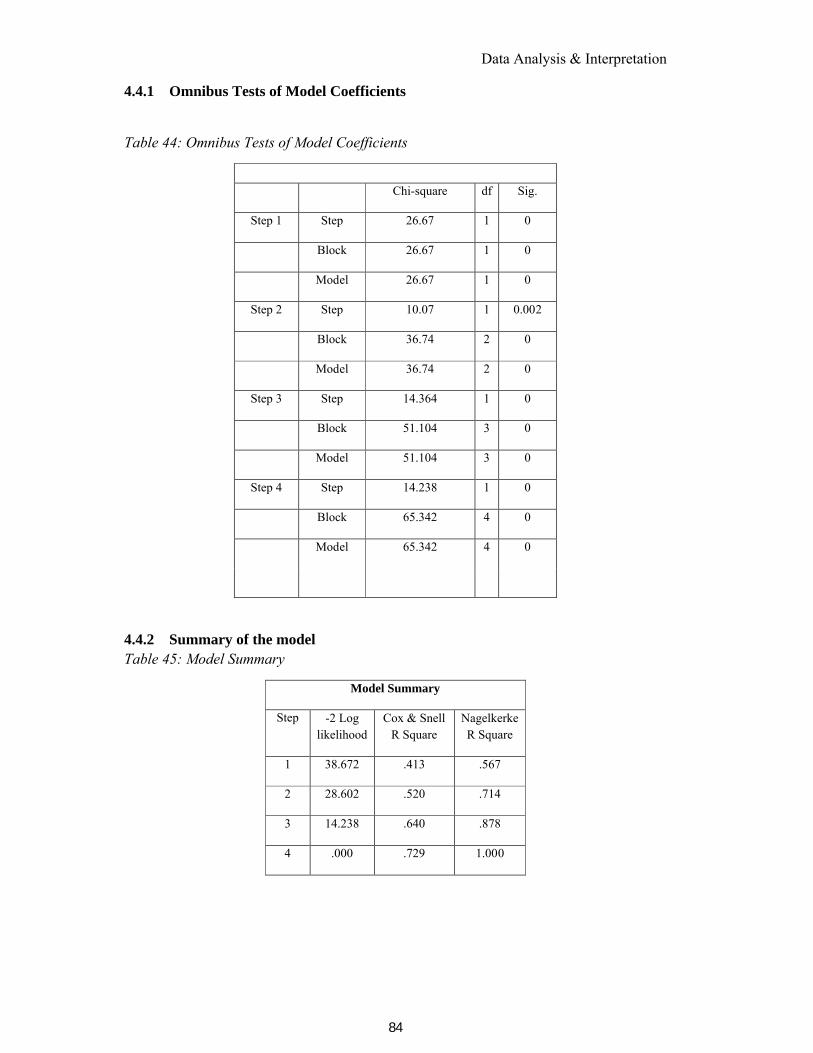
Data Analysis & Interpretation

84

4.4.1 Omnibus Tests of Model Coefficients

Table 44: Omnibus Tests of Model Coefficients

Chi-square df Sig.

Step 1 Step 26.67 1 0

Block 26.67 1 0

Model 26.67 1 0

Step 2 Step 10.07 1 0.002

Block 36.74 2 0

Model 36.74 2 0

Step 3 Step 14.364 1 0

Block 51.104 3 0

Model 51.104 3 0

Step 4 Step 14.238 1 0

Block 65.342 4 0

Model 65.342 4 0

4.4.2 Summary of the modelTable 45: Model Summary

Model Summary

Step -2 Log likelihood

Cox & Snell R Square

Nagelkerke R Square

1 38.672 .413 .567

2 28.602 .520 .714

3 14.238 .640 .878

4 .000 .729 1.000

Data Analysis & Interpretation

85

4.4.3 Hosmer and Lemeshow TestTable 46 : Hosmer and Lemeshow Test

Step Chi-square Df Sig.

1 5.773 8 .673

2 8.795 8 .360

3 1.497 8 .993

4 .000 4 1.000

The data of above two table represent whether the logistic regression model for measuring

the effect of number of variables on bankruptcy are the predictor of Bankrupt or not. The

Hosmor Lemeshow statistic is 0.000 with significant value 1. The value of Hosmor

Lemeshow chi-square increase at 4th step with significant value more than 0.05, it

indicates that 4th model is best. The -2 log likelihood statistic (LL) is 0.000, chi-square

value of omnibus test is 65.342 and their significant value 0.000 (p<.05) with 4 degrees of

freedom. The results of goodness of fit test shown in table (Model summary) indicated

that the logistic regression model is very good fit.

There are five indicators shows in above table that model fitted very well. The -2 LL is

continues increase up to four steps, indicate best model. The value of Cox Snell

increases indicated that relationship between number of variables and risk tolerance

decrease with steps and it shows 72% relationship. The value of Nagelkerke also

increase with steps indicated that 100% relationship between Bankruptcy and predictor

variables. The value of chi-square decreases which indicated that the model is fit in terms

of categorizes the different ratio into bankruptcy and non-bankruptcy and at the last

statistical significant value of four steps is less than 0.05.

4.4.4 Classification Matrix for the bankruptcy model with Ohlson ModelTable 47: Classification Matrix for the bankruptcy model with Ohlson Model

Classification Table

Observed Predicted

O score

Percentage CorrectBankrupt

not bankrupt

Data Analysis & Interpretation

86

Step 1 O score bankrupt 12 6 66.7

not bankrupt

3 29 90.6

Overall Percentage 82.0

Step 2 O score bankrupt 16 2 88.9

not bankrupt

3 29 90.6

Overall Percentage 90.0

Step 3 O score bankrupt 16 2 88.9

not bankrupt

1 31 96.9

Overall Percentage 94.0

Step 4 O score bankrupt 18 0 100.0

not bankrupt

0 32 100.0

Overall Percentage 100.0

The success of logistic regression can be assessed by looking at the classification table.

This table shows the estimation about whether model has correctly classified the

bankruptcy or not. The columns indicate predicted value and rows indicate actual value of

two categories step wise. At the first step, the bankrupt category is classified 67% and not

bankrupt category by 91% correctly. The model increase correct classification as it

increases the steps. At the forth step, the bankrupt category is 100% and not bankrupt

category by 100% correctly classified. The overall correct classification of model is 100

%.

4.4.5 Descriptive statistics for the estimation sample

Table 48: Descriptive statistics for the estimation sample

Accounting variable Bankrupt firms Non Bankrupt firms

Mean St.dev Mean St.dev P value

ALTMAN

WC/TA 0.0045 0.2997 0.2177 0.2011 0.014

Data Analysis & Interpretation

87

RE/TA 0.01872 0.5340 0.5690 0.1737 0.0003

EBIT/TA 0.0274 0.6951 0.2349 0.1726 0.000

DEBT/EQUITY 0.3421 0.5385 5.1974 3.6325 0.000

SALES/TA 0.4808 0.3220 1.1363 0.7738 0.001

OHLSON

SIZE 2.3589 0.5761 1.3343 0.8369 0.000

TL/TA 1 0.0000 1 0.0000

WC/TA 0.2205 0.1746 0.0332 0.3190 0.026

CL/CA 0.6143 0.2371 2.1344 6.2324 0.308

OENEG 0.0000 0.0000 0.0000 0.0000

NI/TA 0.1563 0.1371 0.0032 0.06719 0.000

FU/TL 0.2252 0.1590 0.0279 0.0826 0.000

INTWO 0.0000 0.0000 0.1875 0.3966 0.052

CHIN 0.0305 0.2741 -0.1856 0.5443 0.123

P value of pooled t-test (with a confidence level of 95%) of differences in variable means

between the bankrupt and non-bankrupt groups. The p value is greater than the α-level of

0.05, it indicates the null hypothesis is not rejected i.e. There is no significant difference

between mean of Bankrupt and non Bankrupt category and the p value is less than the α-

level of 0.05, it indicates the null hypothesis is rejected i.e. There may be significant

difference between mean of Bankrupt and non Bankrupt category.

Data Analysis & Interpretation

88

4.4.6 Classification matrix for the bankruptcy model (Ohlson Model) with original statistical technique

Table 49: Classification matrix for the bankruptcy model using Ohlson Model with original statistical technique

Classification Table

Observed Predicted

Decision O score

Percentage CorrectBankrupt

not bankrupt

Ohlson model

O score Bankrupt 18 0 100.0

not bankrupt

0 32 100.0

Overall Percentage 100.0

4.4.7 Classification matrix for the bankruptcy model (Altman Model) with original statistical technique

Table 50 : Classification matrix for the bankruptcy model using Altman Model with original statistical technique

Classification Results

Status of companyPredicted Group Membership

TotalSafe Grey Distress

Altman

Count

Safe 13 5 1 19

Grey 0 10 1 11

Distress 0 3 17 20

%

Safe 68.4 26.3 5.3 100.0

Grey .0 90.9 9.1 100.0

Distress .0 15.0 85.0 100.0

Data Analysis & Interpretation

89

4.4.8 Overall Accuracy of the Model

Table 51: Overall Accuracy of the Model

Model Accuracy

Altman 80%

Ohlson 100%

The model of Altman (1968) has an overall accuracy rate of 80%. The overall accuracy rate of this model is low as compared to the Ohlson. Furthermore, the model of Ohlson (1980) has an overall accuracy rate of 100 %.

Findings & Conclusions

90

CHAPTER 5

Findings and Conclusion

5 Findings and Conclusion

5.1 Findings

The researcher has done descriptive statistics, Discriminant Analysis, One way ANOVA and

Post Hoc Tests. The researcher has found different points based on data analysis by using

various statistical tools.

5.1.1 ANOVA

There is statistical significant difference on working capital to total assets between all selected

units under different status of company.

There is statistical significant difference on Retained Earnings to total assets between all selected

units under different status of company.

There is statistical significant difference on Earnings before Interest & Taxto total assets

between all selected units under different status of company.

There is statistical significant difference on Market value of Equity Shares to Total Liabilities

between all selected units under different status of company.

There is statistical significant difference on Net Sales to Total Assets between all selected units

under different status of company.

5.1.2 Post Hoc Tests

There is statistical significant difference on working capital to total assets between Safe and

Distress Company.

There is statistical significant difference on Retained Earnings to total assets between Safe and

Distress Company and there is statistical significant difference on Retained Earnings to total

assets between Grey and Distress Company.

Findings & Conclusions

91

There is statistical significant difference on Earnings before Interest & Tax to total assets

between all status i.e. between Safe and Grey Company; Safe and Distress Company and Grey

and Distress Company

There is statistical significant difference on Market value of Equity Shares to Total Liabilities

between all status i.e. between Safe and Grey Company; Safe and Distress Company and Grey

and Distress Company.

There is statistical significant difference on Net Sales to Total Assets between Safe and Distress

Company and Grey and Distress Company.

5.1.3 Discriminant Analysis

Discriminant Analysis is used primarily to predict membership in two or more mutually

exclusive groups. Discriminant analysis revealed that all variable had significant differences

between Safe, Grey and financially Distress Company.

Researcher is using only three groups here, namely ‘Safe’ ,’Grey’ and ‘Distress’, From the

Discriminant Analysis, researcher found the model

Di=-2.475+1.007X1+1.885X2+3.467X3+0.212X4-1.058X5

From the table no.37 it found that DA model accuracy is 68.4% for Safe firms, 26.3% Grey

firms and 5.3% for Distress firms and 84% in total. According to the table no. 38when the

discriminant functions were used to “predict” from the five variables, 84% of the original

grouped cases were correctly reclassified back into their original categories.

5.1.4 Logistic Regression

From the result of logistic regression, it seems that at the first step, the bankrupt category is

classified 67% and not bankrupt category by 91% correctly. The model increase correct

classification as it increases the steps. At the forth step, the bankrupt category is 100% and not

bankrupt category by 100% correctly classified. The overall correct classification of model is

100 %.

5.2 Conclusion

All the objectives mentioned in the thesis are addressed and a new model for evaluating

financial status of the companies is framed by changing coefficient and adding a constant

Findings & Conclusions

92

taking Altman model as base. As with change in business condition, country, time period the

accuracy of the model changes, this model will help stakeholders to know the likelihood of

financial distress of the companies successfully. The thesis reveals that though the above

studied bankruptcy prediction models are different in their statistical techniques but uses the

same profitability and liquidity ratio to predict bankruptcy. Author compared Ohlson’s

(1980) model to Altman’s (1968) model and concluded that Ohlson model has a higher

predictive ability. Thus it can be said that the explanatory variables of this model are good

predictor of the likelihood of bankruptcy. As a remark, researcher would like to add that the

purpose was not to find the best predictor model of failure but rather to investigate the

predictive ability of model.

5.3 Achievements with respect to Objectives

All the objectives laid down are met by researcher and are shown in below listed table

Table 52: Achievements with respect to Objectives

Objectives Achievements SignificanceTo conduct secondary

study for understanding

sickness prediction models

formulated by earlier

researchers, number of

parameters used by them,

the mathematical

treatment given in the

model and the predicting

accuracy of them.

Different sickness

prediction models were

studied ranging from

conventional models like

Altman, Ohlson to newer

models using neural

network and machine

learning etc.

The mathematical approach taken by different

models was understood. Also the variables used

by different models and its effect on industrial

health were deliberated.

To develop the model based on accounting information that predict the bankruptcy

Original Altman Model was modified by taking the original variables but calculated usingDiscriminant Analysisnew coefficient and also constant.

It is used primarily to predict membership in two or more mutually exclusive groups.

Model :

Di=-2.475+1.007X1+1.885X2+3.467X3+0.212X4-

1.058X5

DA model accuracy is 68.4% for Safe firms, 26.3% Grey firms and 5.3% for Distress firms and 84% in total.84% of the original grouped cases were correctly

reclassified back into their original categories.

Findings & Conclusions

93

To investigate financial ratio of selected companies and identify which ratios contribute to the downfall or bankruptcy.

Ohlson model and Logistic Regression was applied to investigate the ratios responsible for downfall of the companies.

At the first step, the bankrupt category is

classified 67% and not bankrupt category by 91%

correctly. The model increase correct

classification as it increases the steps. At the forth

step, the bankrupt category is 100% and not

bankrupt category by 100% correctly classified.

The overall correct classification of model is 100

%.

To test with past data of selected companies various predictions models and validate the efficacy of the models in predicting the sickness.

Predicting accuracy was checked both with original models as well as modified model.

Model Accuracy

Altman 80%

Ohlson 100%

To identify the difference in five ratios among safe, distress and grey zone companies.

ANOVA 1. Significant difference between the groups on

working capital to total assets.

2. significant difference between the groups on

Retained Earnings to Total Assets

3. Statistically significant difference between the

groups on Market value of Equity Shares to Total

Liabilities.4. Statistically significant difference between the

groups on Net Sales to Total Assets

Post Hoc 1.significant difference between the Safe and

Distress company on working capital to total

assets;

2. Significant difference between the Safe and Distress company on Retained Earnings to Total Assets.

3. significant difference between all status i.e.

between Safe and Grey Company; Safe and

Distress Company and Grey and Distress

Company on Market value of Equity Shares to

Total Liabilities.

4. significant difference between the Safe and

Distress Company and Grey and Distress

Company on Net Sales to Total Assets

Findings & Conclusions

94

5.4 Original Contribution made by the thesisTable 53: Differentiating Factors between the Developed Models and Proposed Model

Sr. No.

Parameters Contribution by thesis Differentiating factor

1 Ease of Computation Researcher has used five variables that are similar toAltman model but the model has been reframed and new coefficients and constant has been computed.

Many studies uses large number of variables and the computational methodologies are very complex.

2 Ease of Interpretation Uses same scale as Altman for interpretation so very easy to interpret.

Same as Altman model

3 Significance of the Variables Out of five variables in the mode 3 are found to be significant in distinguishing the category of companies and 2 were not significant.

This concludes that the non significant variables can be dropped out.

4 Accuracy For Discriminant Analysis the accuracy is 80% but by logistic regression the accuracy is almost 100% by increasing the step to three levels.

All other models have accuracy ranging from 84% -96%.

5 Relevance to Indian Companies The study focuses on Indian companies. Very rare studies exist for Indian Companies.

Other researchers have focussed on non Indian companies.

5.5 Future Scope of the study:1. The study is based on financial data of listed manufacturing companies in the organised

sector and does not include unorganised sector.2. Units run by other forms such as partnership, proprietorship, cooperative society etc have

not been studied.3. Non financial aspects are open field for future study.4. Area of future research would be to extend the analysis to other statistical techniques

References

95

References

Aktan, S. (Sep 2011). Early Warning System for Bankruptcy Prediction (Unpublished doctoral dissertation). Wilhelmshaven. .

Aktan, S. (2011, 12 2). Early warning system for bankruptcy : Bankruptcy Prediction.

Aliakbari, s. Prediction of Corporate Bankruptcy for the UK firms in Manufacturing Industry.Brund University, Department of economics andFinance.

Anghelessai, A. &. (2005). Bankruptcy Prediction in the high- tech industry. Retrieved from SSRN: http://ssrn.com/abstract=649501.

Anjum, s. (2016). Business Bankruptcy Prediction Models: A significant study of the Altman's Z score Model. Asian Journal of Management, 3 (1), 212-219.

Antonio E. Bernardo, A. F. ( 2015, October). Capital Structure with Endogenous Liquidation Values. SSRN .

Avenhuis, J. O. Testing the generalizability of the bankruptcy prediction models of Altman, Ohlson & Zmijewski for dutch listed and large non -listed firms. . Netherlands: University of twente Enschede.

Avenhuis, J. O. ( November2013). Testing the generalizability of the bankruptcy prediction models of Altman, Ohlson & Zmijewski for dutch listed and large non -listed firms.. University of twente Enschede, the , Netherlands.

Bakri, G. (2014). Analysis of Financial Strength of Select Firms from Indian Textiles Industry using Altman's Z Score Analysis. . International Journal of Research in Management, Social Science & Technology, 5 (5), 1-11.

Bapat, V. &. (2016). Comparison of Bankruptcy Prediction Models: Evidence from India. . Accounting and Finance Reserach, 3 (4), 91-98.

Bapat, V. &. (2016). Comparison of Bankruptcy Prediction Models: Evidence from India. . Accounting and Finance Reserach, 3 (4), 91-98.

Bauer, J. (2011-12). Bankruptcy Risk Prediction & Pricing Unravelling The Negative Distress Risk Premium. . Cranfield School of Management.

Baxter R.A, G. M. (n.d.). Predictive model of insolvency risk of Australian Corporation.

Bellovary, J. G. (2007). A Review of Bankruptcy Prediction Studies: 1930-Present. Journal of Financial Education, 33, 1-21.

BYM.K.ODIPO, M. a. (2008). Evaluation of applicability of Altman’s Revised model in prediction of financial distress: A case of companies quoted in Nirobi stock exchange.

References

96

Chotalia, P. (. (2016). Evaluation of Financial Health of Sampled Private Sector Banks with Altman Z -Score Model. . International Journal of Research in Management, Science & Technology, 2 (3),42-46.

Dr. Florence Memba, A. N. (2013). Causes of Financial Distress: A Survey of Firms Funded by Industrial and Commercial Development Corporation in Kenya. Interdisciplinary Journal Of Contemporary Research In Business, 4 (12), 1171-1184.

Dr. Radha Ganesh Kumar, K. k. (2016). A Comparison of Bankruptcy models. International Journal of Marketing Financial Services & Management Research, 1 (4), 76-86.

Edward Altman, E. H. (2005). Corporate Financial Distress and Bankruptcy.

Eni, N. (2015). Bankruptcy and The Altman Models: Case of Albania. Annals of Faculty of Economics, University of Oradea, 1 (1), 839-845.

Gerittsen, P. (2015, Sep). Accuracy rate of Bankruptcy Prediction models for the Dutch Professional Football Industry. University of Twente, Netherlands.

Gharaibeh, M. S. (2013). The Applicability of Corporate Failure Models to Emerging Economies Evidence from Jordon. Interdisciplinary Journal of Contemporary Research Business, 5 (4), 313-323.

Goyal, D. A. (2015). An Empirical case study on Prediction of Corporate failure in the selected industrial Unit in India. . International Journal of Business Research & Management, 4 (4), 132-137.

Gupta, V. (2014). An Empirical Analysis of Default Risk for Listed Companies in India: A Comparison of Two Prediction Models. . International Journal Of Business & Management, 9 (9), 223-234.

Hayes, S. K. (2015). A study of efficacy of Altman's Z to predict Bankruptcy of speciality Retail firms doing businesss in Contemporary times. . Economics & Business Journal: Inquiries & Perspectives, 3 (1), 130-134.

Jayadev, M. (2006). Predictive power of Financial Risk Factors: An Empirical analysis of Default Companies. . Vikalpa, 31 (3), 45-56.

Junare S.O, P. A. (2012). Predicting corporate Bankruptcy using Financial ratios: An empirical analysis: Indian Evidence from 2007-10. GFJMR, 4, 1.

Junare, S. O. (2012). Predicting Corporate Bankruptcy using Financial Ratios: An Empirical Ananlysis: Indian Evidence from 2007-10. GFJMR, 4, 1-14.

Kordlar, A. E. (2015). COMPARING BANKRUPTCY PREDICTION MODELS IN IRAN. . Business Intelligence Journal, 4 (2), 335-342.

Kristof, T. (2008). Corporate survival and solvency prediction. Budapest.

Lok Sabha passes bill to fast track debt recovery . (2016, Aug 2). The Economic Times , p. Economy.

References

97

M. K., &. D. (2016, February 18). Distress Prediction Model- Model for predicting Bankruptcy in Aviation Industry. . International Journal of Emerging Research in Management and Technology , 15-18.

Michal Karas, M. R. (2017). (2017). The Potential of Dynamic Indicator in Development of the Bankruptcy Prediction Models: the Case of Construction Companies. ,65(2),641652.RetrievedApril30,2017,fromhttps://doi.org/10.1. ActaUniv.Agric.Silvic.MendelianaeBrun, 65, 641-652.

Mihail, D. (2010). The effectiveness of Altman’s three models in bankruptcy forecast for private hotels in Greece.

Ng Kim Soon, A. A. (n.d.). Applicability of Altman’s Revised Model in predicting Financial Distress: A case of PN17 companies quoted in Malaysian Stock Exchange.

Pandey, D. V. (2013). Measuring Financial Soundness of Indian Telecom Companies- A Comparative Analysis. . The International Journal of Management, 2 (2), 1-13.

Panigrahy, D. &. (1993). Predicting Corporate Sickness Using Cash Flow Analysis. . Vikalpa , 18(3), 13-19.

Pervan, I. P. (2016). Prediction of Company Bankruptcy Using Statistical Techniques- Case of Croatia. . Croatian Operational Research Review, 2, 158-167.

peter Lindner, S. E. (December 2014). corporate Vulnerabilities in India and Bank's Loan Performance. working paper, IMF, Asia and Pacific Department.

Pradhan, R. (. (2016). Z-score Estimation for Indian Banking Sector. . International Journal of Trade, Economics and Finance, 5 (6), 516-520.

Ramaratnam, M. &. (2013). Impact of Financial Strength on Leverage: A Study with special Reference To Select Companies in India. International Monthly Referred Journal In Management & Technology, 2, 34-38.

Ray, S. (2011). Assessing Corporate Financial Distress in Automobiles Industry of India: An Application of Altman's Model. Research Journal of Finance and Accounting, 2 (3), 155-168.

Rohit Bansal, H. b. (2017). Financial Distress Prediction of Indian Companies: Future Perspectives. International Journal of Economic Research, 14 (4), 173-181.

S Christina, S. &. (2012). Evaluating Financial Health of Pharmaceutical Industry in India through Z Score model. . International Journal of Social Sciences & Interdisciplinary Research, 1 (5), 25-31.

Sanobar, A. (2012). Business Bankruptcy Prediction models: A Significant study of the Altman's Z score model. . Asian Journal of Management Research, 3 (1), 212-219.

Satish, M. &. (2011). Turnaround Strategy using Altman Model as a Tool in Solar Water Heater Industry in Karnataka. International Journal Of Business & Management, 6 (1), 199-2016.

Sinha, G. Financial Statement Analysis.

References

98

THENMOZHI, S. D. (2017). FINANCIAL HEALTH OF SELECTED IRON AND STEEL COMPANIES IN INDIA - Z SCORE MODEL. . International Journal in Management and Social Science, 3 (12), 278-289.

Vadivu, S. S. (2014). A Study on Financial Health of Select Indian Pharmaceutical Companies. Peer Reviewed International Journal, 2 (9), 1-9.

VenkataRamana, N. A. (2012). Financial Performance and Predicting The Risk Of Bankruptcy: A Case Of Selected Cement Companies In India. International Journal of Public Administration And Management Research, 1 (1), 40-56.

Vineet Agarwal, R. T. (2008). Comparing the performance of market-based and accounting-based bankruptcy. Journal of Banking & Finance, 32 (8), 1541-1551.

wood, A. p. (2012). The Performance of Insolvency Prediction and credit risk models in the UK:A comparative study, Development and wider Application. University of Exeter.

Xavier, B. (2016). Bankruptcy Prediction Model Using Neural Networks. . Accounting and Finance Reserach, 3 (2), 124-128.

99

Papers Published

1. Miss Jaya Kumari P Dakhwani, D. K. (2018). Predicting Financial Distress of S Kumar Nationwide Ltd- A comparision of Altman's Z score model and Ohlson's O score model. IJCESR, 5 (4), 57-61.

2. Miss Jayakumari P Dakhwani, D. K. (2017). Financial Distress Analysis of Selected Indian Pharmaceutical Companies. International Journal of Exclusive Management Research, 7 (10), 16-21.

3. Dakhwani, M. J. (2015). A Case Study on Crisis in Kingfisher Airlines. Interdisciplinary Studies in Management , 227-233.