a study of traffic locality and reliability in peer-to-peer video
TRANSCRIPT
A Study of Traffic Locality and Reliability in
Peer-to-Peer Video Streaming Applications
by
Xiangyang Zhang
A thesis submitted to the
School of Computing
in conformity with the requirements for
the degree of Doctor of Philosophy
Queen’s University
Kingston, Ontario, Canada
April 2012
Copyright c© Xiangyang Zhang, 2012
Abstract
The past decade has witnessed tremendous growth of peer-to-peer (P2P) video stream-
ing applications on the Internet. For these applications, playback smoothness and
timeliness are the two most important aspects of users’ viewing experiences, whereas
the amount of traffic is Internet service providers’ main concern. According to the
playback delay, video streaming can be classified into on-demand streaming, live
streaming, and interactive streaming. P2P live streaming applications typically have
an arbitrary number of users, tens of seconds of playback delay, and a high packet
delivery rate, but their heavy traffic incurs great financial expenditure and threatens
the quality of other services. Interactive streaming applications usually have a small
group size, several hundreds of milliseconds of playback delay, and reasonable traffic
volume, but cannot achieve a high packet delivery rate. The goal of this thesis is to
study traffic locality and reliable delivery of packets in large-scale live streaming and
small-scale interactive streaming applications, while keeping the playback delay well
below the targeted applications’ limits.
For P2P live streaming applications, we first identify “typical” schemes from ex-
isting P2P live streaming schemes, investigate packet propagation behavior and the
impact of neighboring strategies on system performance, and then propose innovative
i

schemes that take both users’ viewing experience and traffic locality into considera-
tion. We show that the network-driven tree-based schemes with the swarming tech-
nique as a re-transmission error-correction mechanism are superior to the data-driven
swarm-based or tree-based schemes, and a properly designed tree-based scheme can
localize the traffic while maintaining a high packet delivery rate.
For interactive streaming applications, we analyze the efficacy of systematic for-
ward error-correction (FEC) codes against the bursty errors of Internet links when
using peers to provide multiple one-hop paths between two communication parties.
We find that although using peers for path diversity often results in a lower post-FEC
packet loss ratio, some conditions do apply. The interplay of a number of factors,
such as the Internet links’ error ratio and burst length and the coding parameters,
determines the performance of FEC. We provide guidelines and computation methods
to determine whether the use of peers for path diversity can be justified.
ii

Acknowledgments
First and foremost I offer my sincerest gratitude to my supervisor, Prof. Hossam
S. Hassanein. His wisdom, knowledge, and rigor inspire me on both an academic and
personal level. I simply could not wish for a better or friendlier supervisor.
I am greatly indebted to my wife, Li Cao. This thesis would not have been possible
without her love, sacrifice, and unconditional support. I also credit our child, Angela,
for amazing me every day.
My deepest gratitude goes to my father, Jilai Zhang, and my mother, Cuixin
Wang. They spared no effort to provide the best possible environment for me to grow
up and they had never complained in spite of all the hardships in their life.
I would like to thank Ahmed Hasswa, Dr. Kashif Ali, Dr. Yik Hung Tam, Dr. Abd-
Elhamid Taha, Michael Liu, Mingyi Zhang, Xianrong Zheng, Abdulmonem Rashwan,
Atef Mohamed, Walid Ibrahim, Mervat Abu-Elkheir, Mahmoud Ouda, Abdulrahman
Abahsain, Ed Elkouche, Khalid Elgazzar and all the members of the School of Com-
puting, especially the Telecommunication Research Lab, at Queen’s University for
their support, friendship and fruitful discussions. Special thanks to Dr. Quanhong
Wang and Dr. Kenan Xu for helping me to settle down in Kingston, and to Dr. Afzal
Mawji for commenting on many of my papers.
iii

I would like to thank the faculty of Queen’s University for their excellent instruc-
tion. Special thanks to Prof. Glen Takahara, whose lessons are the best I have ever
had in my life.
Thanks to Basia Palmer and Debby Robertson for their help in my time of need.
Thanks to Patti Riley for correcting many grammatical errors in this thesis.
Finally, I would like to thank members of the examination committee for their
valuable remarks, and acknowledge with great appreciation the funding provided by
Queen’s University.
Xiangyang Zhang
Kingston, Ontario
April 25, 2012
iv

Statement of Originality
I hereby certify that this Ph.D. thesis is original and that all ideas and inventions
attributed to others have been properly referenced.
Xiangyang Zhang
Feb 8th, 2012
v

vi

List of Acronyms
AS Autonomous System
BGP Border Gateway Protocol
BRAS Broadband Access Server
CAC Connection Admission Control
CDF Cumulative Density Function
CDN Content Delivery Network
DBMST Degree-Bounded Minimum Spanning Tree
DBSPT Degree-Bounded Shortest Path Tree
DHT Distributed Hash Table
DNS Domain Name Service
DV Distance-Vector
DVB Digital Video broadcast
DVMRP Distance-Vector Multicast Routing Protocol
FEC Forward Error-Correction
GOP Group of Pictures
IGMP Internet Group Management Protocol
ISP Internet Service Provider
LAN Local Area Network
vii
MDC Multiple Description Coding
MOSPF Multicast Open Shortest Path Forwarding
MPEG Motion Picture Expert Group
MST Minimum Spanning Tree
MTBG Mean Time Between Glitches
NAL Network Abstraction Layer
NAT Network Address Translation
PDF Probability Density Function
PIM Protocol Independent Multicast
RIP Routing Information Protocol
RP Rendezvous Point
RTP Real-time Transportation Protocol
RTSP Real-Time Streaming Protocol
SAP Session Announcement Protocol
SDP Session Description Protocol
SIP Session Initiation Protocol
TCP Transport Control Protocol
UDP User Datagram Protocol
VCEG Video Coding Expert Group
VCL Video Coding Layer
VCU Video Control Unit
WMSP Windows Media Streaming Protocol
viii
Co-Authorship
1. X. Zhang, G. Takahara and H. Hassanein, “On the performance of systematic
FEC codes when using dynamic peers for path diversity,” Submitted to Trans-
actions on Networking, pp. 1–12, 2012.
2. X. Zhang and H. Hassanein, “A survey on peer-to-peer video live streaming
schemes—An algorithmic perspective,” Submitted to Computer Networks, pp.
1–30, 2012.
3. X. Zhang and H. Hassanein, “Understanding the impact of neighboring strat-
egy in peer-to-peer multimedia streaming applications,” Submitted to Computer
Communications Special Issue on Smart and Interactive Ubiquitous Multimedia
Services, pp. 1–12, 2012.
4. X. Zhang, G. Takahara and H. Hassanein, “Reliable interactive video streaming
in peer-to-peer networks,” in Proc. Consumer Communication and Networking
Conf. (CCNC) Special Session on Multimedia Content Distribution Networks,
2012, pp. 768–773.
5. X. Zhang and H. Hassanein, “On network utilization of peer-to-peer video live
streaming on the Internet,” in IEEE Int. Conf. on Communications (ICC),
ix

2011, pp. 1–5.
6. X. Zhang and H. Hassanein, “A neighboring strategy for ISP-friendly peer-to-
peer video live streaming,” in IEEE Int. Conf. on Communications (ICC),
2011, pp. 1–5.
7. X. Zhang and H. Hassanein, “Treeclimber: A network-driven push-pull hybrid
scheme for peer-to-peer video live streaming,” in Proc. IEEE Local Computer
Networks (LCN), 2010, pp. 368–371.
8. X. Zhang and H. Hassanein, “Video on-demand streaming on the Internet—A
survey,” in Queen’s Biennial Symposium on Communications (QBSC), 2010,
pp. 88–91.
x

Table of Contents
Abstract i
Acknowledgments iii
Statement of Originality v
List of Acronyms vi
Co-Authorship ix
Table of Contents xi
List of Tables xvi
List of Figures xvii
Chapter 1:
Introduction . . . . . . . . . . . . . . . . . . . . . . . . . . 1
1.1 Motivations and Objectives . . . . . . . . . . . . . . . . . . . . . . . 3
1.2 Thesis Contributions . . . . . . . . . . . . . . . . . . . . . . . . . . . 7
1.3 Thesis Outline . . . . . . . . . . . . . . . . . . . . . . . . . . . . . . . 10
xi
Chapter 2:
Background . . . . . . . . . . . . . . . . . . . . . . . . . . 12
2.1 Video Streaming On the Internet . . . . . . . . . . . . . . . . . . . . 12
2.2 Video Coding . . . . . . . . . . . . . . . . . . . . . . . . . . . . . . . 18
2.2.1 Block-Based Motion-Compensated Predictive Coding . . . . . 19
2.2.2 H.264/MPEG-4 AVC . . . . . . . . . . . . . . . . . . . . . . . 22
2.2.3 Multiple Layered Coding . . . . . . . . . . . . . . . . . . . . . 24
2.3 P2P Networks . . . . . . . . . . . . . . . . . . . . . . . . . . . . . . . 24
2.3.1 Locating and Routing . . . . . . . . . . . . . . . . . . . . . . 26
2.3.2 Retrieving Data Objects . . . . . . . . . . . . . . . . . . . . . 29
2.4 P2P Live Streaming . . . . . . . . . . . . . . . . . . . . . . . . . . . 30
2.4.1 Classification . . . . . . . . . . . . . . . . . . . . . . . . . . . 30
2.4.2 Representative Schemes . . . . . . . . . . . . . . . . . . . . . 37
2.5 Traffic Locality in P2P Video Streaming Applications . . . . . . . . . 44
2.5.1 Finding the Minimum Cost Tree . . . . . . . . . . . . . . . . . 45
2.5.2 Finding Nearby Peers . . . . . . . . . . . . . . . . . . . . . . . 48
2.6 Reliability in P2P Video Streaming Applications . . . . . . . . . . . . 49
2.6.1 Error-Correction . . . . . . . . . . . . . . . . . . . . . . . . . 50
2.6.2 Fast Tree-Repairing . . . . . . . . . . . . . . . . . . . . . . . . 52
2.7 Performance Metrics . . . . . . . . . . . . . . . . . . . . . . . . . . . 53
Chapter 3:
Understanding Neighboring Strategies . . . . . . . . . . 56
3.1 Introduction . . . . . . . . . . . . . . . . . . . . . . . . . . . . . . . . 56
3.2 Related Work . . . . . . . . . . . . . . . . . . . . . . . . . . . . . . . 58
xii
3.3 Typical Swarm-Based and Tree-Based Schemes . . . . . . . . . . . . . 59
3.3.1 Overlay Construction . . . . . . . . . . . . . . . . . . . . . . . 60
3.3.2 Typical Swarm-Based (TS) Scheme . . . . . . . . . . . . . . . 61
3.3.3 Typical Tree-Based (TT) Scheme . . . . . . . . . . . . . . . . 62
3.4 Simulation Study . . . . . . . . . . . . . . . . . . . . . . . . . . . . . 63
3.4.1 Simulation Setting . . . . . . . . . . . . . . . . . . . . . . . . 64
3.4.2 Simulation Results . . . . . . . . . . . . . . . . . . . . . . . . 65
3.5 Analysis of Chunk Propagation . . . . . . . . . . . . . . . . . . . . . 71
3.5.1 Chunk Propagation in Typical Swarm-Based (TS) Scheme . . 72
3.5.2 Chunk Propagation in Typical Tree-Based (TT) Scheme . . . 75
3.5.3 Impact of Multiple Paths and Limited Upload Capacity . . . . 77
3.6 Analysis of the Impact of Overlays . . . . . . . . . . . . . . . . . . . 79
3.6.1 Properties of Random and Nearby Overlays . . . . . . . . . . 79
3.6.2 Impact of Neighbor-With-Nearby-Peers Strategy . . . . . . . . 84
3.7 Summary . . . . . . . . . . . . . . . . . . . . . . . . . . . . . . . . . 86
Chapter 4:
ISP-Friendly P2P Live Streaming . . . . . . . . . . . . . 88
4.1 Introduction . . . . . . . . . . . . . . . . . . . . . . . . . . . . . . . . 88
4.2 Related Work . . . . . . . . . . . . . . . . . . . . . . . . . . . . . . . 89
4.3 Desired Neighboring Overlay and Propagation Tree . . . . . . . . . . 90
4.4 Overlay Construction . . . . . . . . . . . . . . . . . . . . . . . . . . . 91
4.5 Tree Building . . . . . . . . . . . . . . . . . . . . . . . . . . . . . . . 95
4.5.1 Determining Parent–Child Relationships . . . . . . . . . . . . 96
4.5.2 Avoiding Forwarding Loops and Duplicated Chunks . . . . . . 98
xiii

4.5.3 Fast Tree Repairing . . . . . . . . . . . . . . . . . . . . . . . . 99
4.6 Error-Correction . . . . . . . . . . . . . . . . . . . . . . . . . . . . . 100
4.7 Performance Evaluation . . . . . . . . . . . . . . . . . . . . . . . . . 101
4.7.1 Simulation Setting . . . . . . . . . . . . . . . . . . . . . . . . 103
4.7.2 TreeClimber vs. Typical Tree-Based (TT) Scheme . . . . . . . 103
4.7.3 Hiarchical Overlay vs. Random and Small-World Overlays . . 106
4.7.4 Impact of Long Edges . . . . . . . . . . . . . . . . . . . . . . 112
4.7.5 Trade-Off Between the Playback Delay and Delivery Rate . . 113
4.8 Summary . . . . . . . . . . . . . . . . . . . . . . . . . . . . . . . . . 114
Chapter 5:
FEC Performance in Interactive Streaming . . . . . . . 115
5.1 Introduction . . . . . . . . . . . . . . . . . . . . . . . . . . . . . . . . 115
5.2 Related Work . . . . . . . . . . . . . . . . . . . . . . . . . . . . . . . 118
5.3 Network Model . . . . . . . . . . . . . . . . . . . . . . . . . . . . . . 120
5.3.1 P2P Network Model . . . . . . . . . . . . . . . . . . . . . . . 120
5.3.2 Path Diversity . . . . . . . . . . . . . . . . . . . . . . . . . . . 122
5.4 FEC Performance with the Direct Path . . . . . . . . . . . . . . . . . 124
5.4.1 Loss Model for Unicast Channels . . . . . . . . . . . . . . . . 125
5.4.2 Post-FEC Loss Ratio . . . . . . . . . . . . . . . . . . . . . . . 126
5.5 FEC Performance With a Sufficient Number of Disjoint CO Channels 127
5.5.1 Concatenation of Unicast Channels . . . . . . . . . . . . . . . 128
5.5.2 Loss Model for CO Channels . . . . . . . . . . . . . . . . . . . 129
5.5.3 Post-FEC Loss Ratio . . . . . . . . . . . . . . . . . . . . . . . 131
5.5.4 Numerical Results . . . . . . . . . . . . . . . . . . . . . . . . 131
xiv

5.6 FEC Performance With a Limited Number of Disjoint CO Channels . 136
5.6.1 Subchannels of a CO Channel . . . . . . . . . . . . . . . . . . 136
5.6.2 Post-FEC Loss Ratio . . . . . . . . . . . . . . . . . . . . . . . 137
5.6.3 Numerical Results . . . . . . . . . . . . . . . . . . . . . . . . 138
5.7 FEC Performance With a Large Number of Non-Disjoint CO Channels 140
5.7.1 Loss Model For Non-Disjoint CO Channels . . . . . . . . . . . 141
5.7.2 Post-FEC Loss Ratio . . . . . . . . . . . . . . . . . . . . . . . 143
5.7.3 Numerical Results . . . . . . . . . . . . . . . . . . . . . . . . 145
5.8 Impact of Heterogeneous Channels and Absence of Substrate Path
Knowledge . . . . . . . . . . . . . . . . . . . . . . . . . . . . . . . . . 145
5.8.1 Heterogeneous Channels . . . . . . . . . . . . . . . . . . . . . 145
5.8.2 Random Channel Forwarding . . . . . . . . . . . . . . . . . . 148
5.9 Summary . . . . . . . . . . . . . . . . . . . . . . . . . . . . . . . . . 150
Chapter 6:
Conclusions and Future Directions . . . . . . . . . . . . . 152
6.1 Conclusions . . . . . . . . . . . . . . . . . . . . . . . . . . . . . . . . 152
6.2 Future Directions . . . . . . . . . . . . . . . . . . . . . . . . . . . . . 156
Bibliography . . . . . . . . . . . . . . . . . . . . . . . . . . . . . . . . . 159
Appendix A:
Non-Systematic FEC Performance . . . . . . . . . . . . 172
Appendix B:
Frossard’s Method . . . . . . . . . . . . . . . . . . . . . 175
xv

List of Tables
2.1 Comparison of DHT Algorithms . . . . . . . . . . . . . . . . . . . . . 28
2.2 Taxonomy of P2P Live Streaming Schemes . . . . . . . . . . . . . . . 37
3.1 System Parameters and Default Values . . . . . . . . . . . . . . . . . 61
3.2 Average Playback Delays . . . . . . . . . . . . . . . . . . . . . . . . . 67
3.3 Notations Used in Propagation and Overlay Model . . . . . . . . . . 72
4.1 System Parameters and Default Values . . . . . . . . . . . . . . . . . 92
4.2 Average Propagation Tree and SPT Height . . . . . . . . . . . . . . . 108
5.1 Parameters . . . . . . . . . . . . . . . . . . . . . . . . . . . . . . . . 123
xvi

List of Figures
2.1 Video streaming protocol stack . . . . . . . . . . . . . . . . . . . . . 14
2.2 Three approaches to distributing video packets from a video source to
receivers on the Internet. The number on a link denotes its cost. . . . 16
2.3 Block-based motion-compensated predictive encoding and decoding . 20
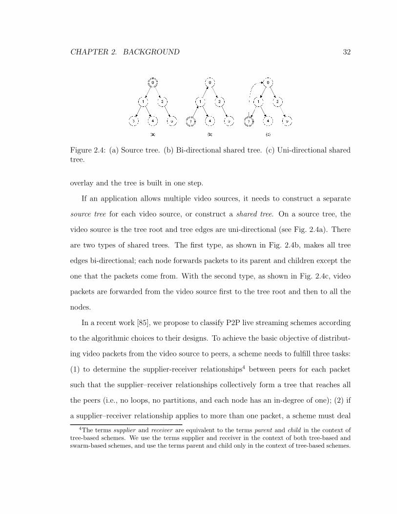
2.4 (a) Source tree. (b) Bi-directional shared tree. (c) Uni-directional
shared tree. . . . . . . . . . . . . . . . . . . . . . . . . . . . . . . . . 32
2.5 Taxonomy with respect to tree-building algorithms . . . . . . . . . . 33
2.6 Impact of the two types of cost functions in the recursive method. The
number on a link denotes its cost. . . . . . . . . . . . . . . . . . . . . 46
3.1 Average overlay and propagation tree edge cost in TT and TS, nor-
malized with the average cost of all the pair-wise edges between peers
in the system. . . . . . . . . . . . . . . . . . . . . . . . . . . . . . . . 66
3.2 Cumulative distribution of peers’ root path length in TS when each
peer’s upload capacity is set to its degree minus 1. The y-axis is the
fraction of peers whose root path length is no more than the value
plotted on the x-axis. . . . . . . . . . . . . . . . . . . . . . . . . . . . 68
3.3 Propagation tree height in TT and TS on random overlay. . . . . . . 69
xvii
3.4 Peers’ chunk loss rate when substrate Internet links are error-free. The
y-axis is the cumulative fraction of peers whose chunk loss rate is less
than the value on the x-axis. . . . . . . . . . . . . . . . . . . . . . . . 70
3.5 Peers’ chunk loss rate when substrate Internet links have an error rate
of 1%. The y-axis is the cumulative fraction of peers whose chunk loss
rate is less than the value on the x-axis. . . . . . . . . . . . . . . . . 71
3.6 Two disjoint paths with n and m hops, n > m. The leftmost peer is
denoted as x0 and y0 and the rightmost peer as xn and ym for convenience. 72
3.7 Peer distribution on nearby overlay . . . . . . . . . . . . . . . . . . . 82
4.1 Hierarchical overlay. Higher layers contain peers with higher band-
widths. Layer 1 contains short edges; upper layers contain rewired
edges. . . . . . . . . . . . . . . . . . . . . . . . . . . . . . . . . . . . 90
4.2 Normalized probability that a long edge exists between two peers. The
x and y axes are normalized bandwidth and distance between the two
peers, β = 1, κ = 2 . . . . . . . . . . . . . . . . . . . . . . . . . . . . 94
4.3 Neighboring overlay and subscription tree. The number at each peer
indicates the peer’s upload bandwidth. . . . . . . . . . . . . . . . . . 95
4.4 Normalized propagation tree cost of the hierarchical overlay when the
bandwidth setting is U(0, 6). . . . . . . . . . . . . . . . . . . . . . . . 104
4.5 Average propagation tree height on the hierarchical overlay when the
bandwidth setting is U(0, 6). . . . . . . . . . . . . . . . . . . . . . . . 104
4.6 Playback delay CDF on the hierarchical overlay when the bandwidth
setting is U(0, 6). . . . . . . . . . . . . . . . . . . . . . . . . . . . . . 105
xviii

4.7 Delivery-rate-user-ratio on the hierarchical overlay when the band-
width setting is U(0, 6). . . . . . . . . . . . . . . . . . . . . . . . . . 106
4.8 Normalized propagation tree cost of the hierarchical overlay, small-
world overlay, and random overlay. . . . . . . . . . . . . . . . . . . . 107
4.9 Playback delay CDF on the hierarchical overlay, small-world overlay,
and random overlay. . . . . . . . . . . . . . . . . . . . . . . . . . . . 110
4.10 Delivery-rate-user-ratio on the hierarchical overlay, small-world over-
lay, and random overlay. . . . . . . . . . . . . . . . . . . . . . . . . . 111
4.11 Impact of fraction of rewired edges on the hierarchical overlay when
the bandwidth setting is U(1, 9). . . . . . . . . . . . . . . . . . . . . . 112
4.12 Impact of playback delay . . . . . . . . . . . . . . . . . . . . . . . . . 113
5.1 Network model. The sender encodes k = 7 original packets into an
FEC block of size n = 8 by appending an FEC packet and sends
encoded packets via N channels in a round-robin fashion. The receiver
can reproduce all the original packets if no more than n−k = 1 packet
is lost in transmission. . . . . . . . . . . . . . . . . . . . . . . . . . . 121
5.2 The number of unique IP addresses at each hop to the 200 most popular
websites from a residential user and a campus user. . . . . . . . . . . 124
5.3 Loss model for unicast channels . . . . . . . . . . . . . . . . . . . . . 125
5.4 Loss model for CO channels . . . . . . . . . . . . . . . . . . . . . . . 129
5.5 Post-FEC loss ratio when using sufficient CO channels (N ≥ n). Each
CO channel has the same parameters p and q as the direct path (bench-
mark). . . . . . . . . . . . . . . . . . . . . . . . . . . . . . . . . . . . 133
xix

5.6 Post-FEC loss ratio when using sufficient CO channels (N ≥ n). Each
of the two segments of a CO channel has the same parameters p and q
as the direct path (benchmark). . . . . . . . . . . . . . . . . . . . . . 135
5.7 Post-FEC loss ratio when using limited CO channels (N < n). Each
CO channel has the same parameters p and q as the direct path (bench-
mark). . . . . . . . . . . . . . . . . . . . . . . . . . . . . . . . . . . . 139
5.8 Abstract topology when a sender uses a large number of non-disjoint
paths to send packets to a receiver. Dashed lines are error-free virtual
links. . . . . . . . . . . . . . . . . . . . . . . . . . . . . . . . . . . . . 141
5.9 Post-FEC loss ratio when using a large number of non-disjoint CO
channels. Each CO channel has the same parameters p and q as the
direct path (benchmark). The access segment has 2 disjoint paths. . . 144
5.10 Post-FEC loss ratio when using heterogeneous CO channels. Internet
links’ loss ratio e and burst length l are uniformly distributed. . . . . 146
5.11 Comparison of the probability density of the post-FEC loss ratio when
Internet links are homogeneous (e is 1% and l is 2) and heterogeneous
(e is U(0, 2%) and l is U(1, 3). The sender uses N=2 disjoint paths
and k=15. . . . . . . . . . . . . . . . . . . . . . . . . . . . . . . . . . 147
5.12 Post-FEC loss ratio when using a large number of random CO peers.
The fraction of access segments account for β = 0.25 of total packet loss.149
xx

Chapter 1
Introduction
The past decade has witnessed tremendous growth of video streaming applications
on the Internet. More and more people are watching user-generated videos, or
professionally-made news clips and full-time TV shows on the Internet rather than sit-
ting in front of a TV screen, renting movies from an online store rather than going to a
physical movie store, and making video calls over the Internet rather than audio calls
over traditional telephone networks. Increasingly, media companies are making their
content available on the Internet, and telecommunication operators and cable TV
operators are upgrading and consolidating their networks to meet the ever-growing
bandwidth requirement of video streaming applications and to provide bundled In-
ternet, telephone, and IPTV1 services to users. No wonder video streaming traffic
has become the dominant type of traffic on the Internet.
The definitive feature of video streaming is that a video is watched while it is
being downloaded. The delay between the retrieval time and the consumption time,
1IPTV refers to TV services provided over IP networks with guaranteed quality. It differs fromInternet TV, which refers to TV services delivered over the Internet.
1
CHAPTER 1. INTRODUCTION 2
called the buffering delay, has the most significant impact on the streaming technique.
Video streaming is often classified into two categories: on-demand streaming and live
streaming. In on-demand streaming applications, a user plays a video at his or her
own pace and may seek new playback positions while viewing the video. A user
can download the video at a faster rate than the video’s playback rate. The buffering
delay is typically small when the user starts playing a video or seeks a further playback
position in a video, so the user’s request is quickly responded. However, the buffering
delay is large at other times for the purpose of smooth playback. In live streaming
applications, every user plays a video in approximate synchronicity with the video
source, and downloads the video at the video’s playback rate. The buffering delay is
small and constant. In some live streaming applications, such as Internet TV, users
do not interact with the video source, and a buffering delay of several minutes is
acceptable. In other applications, such as online action games, the buffering delay
cannot exceed several hundred milliseconds for the sake of interactivity.
In this thesis, we use the term delay-tolerant live streaming or simply live stream-
ing to refer to streaming applications that can tolerate a buffering delay of several
seconds to several minutes, and the term interactive streaming to refer to streaming
applications that only allow a sub-second buffering delay. Video communications,
such as video telephony and conferencing, are inherently streaming and interactive
by nature. Live streaming applications may have an arbitrary group size. For exam-
ple, in Internet TV applications, there may be hundreds of thousands of receivers in
a single channel. Interactive streaming applications typically have a small number of
receivers, and in some cases, only one receiver. This thesis focuses on the two most
common scenarios—large-scale live streaming applications where there are thousands
CHAPTER 1. INTRODUCTION 3
or more users and small-scale interactive streaming applications with several or tens
of users.
A video streaming application may employ the client/server (C/S) model or the
peer-to-peer (P2P) model. In the C/S model, there exists a video server (or server
farm) and every user downloads a video from the video server. In the P2P model, a
user is both a client and a server. A user downloads a video from some other users in
parts (each part from different users), and in the meantime, uploads the video parts
they have to the other users. In large-scale live streaming applications, the C/S model
requires enormous processing power from the video server and the bandwidth of the
Internet, and both incur heavy financial expenditure. The P2P model is attractive
due to its limited requirements of the video server’s processing power and bandwidth
of the Internet. Interactive streaming applications typically use the C/S model, but
may use P2P networks to connect users located behind a firewall or network address
translation (NAT) device. These applications may also use P2P networks to provide
multiple paths between a sender and a receiver for higher reliability, or to organize
users in applications with small group sizes but large numbers of groups. For example,
Skype organizes users into a P2P network and selects some users to be super-nodes to
connect the users behind NATs. This thesis focuses on video streaming applications
that use P2P networks.
1.1 Motivations and Objectives
For P2P live and interactive streaming applications, the smoothness and timeliness of
playback are the two most important aspects of users’ viewing experiences, whereas
the amount of Internet traffic is the main concern of Internet service providers (ISPs).

CHAPTER 1. INTRODUCTION 4
The smoothness of playback is measured by the packet loss rate perceived by a user’s
media player (i.e., after error correction). The timeliness of the playback is mea-
sured by the playback delay, which is the lag from the time a video frame appears at
the video source to the time the video frame is played at a receiver. In P2P video
streaming applications, packets may be lost due to Internet link errors. When a video
source delivers packets to a receiver via other peers, packets may also be lost due to
the churn 2 of intermediate peers. The Internet only provides best-effort delivery of
IP packets. A packet loss rate of several percent is not rare for Internet links. An
application itself needs to correct transmission errors, or it may rely on the transport
control protocol (TCP) to do so. Error correction techniques include re-transmission
and coding. The re-transmission method has little overhead but introduces at least
several seconds of delay. The coding method can be used for applications that only
tolerate a delay of several hundred milliseconds. Coding may be done at the source or
at the channel. Source coding (i.e., video coding), such as multiple description cod-
ing (MDC), has many attractive features but incurs significant coding overhead [19].
Channel coding, sometimes called forward error-correction (FEC) coding, is the most
widely used error correction technique on noisy channels in real-time communications.
Its coding delay is determined by the coding block size, and its efficacy depends on
the coding redundancy and error patterns.
The Internet routes packets along the shortest IP paths between two hosts. How-
ever, in P2P video streaming applications, especially large-scale P2P live streaming
applications where a video source delivers packets to a large number of receivers, the
set of paths a packet propagates from the video source to receivers is a tree from the
perspective of the application layer. We call this tree the packet’s propagation tree.
2Peers’ departures and arrivals are collectively called peer churn.
CHAPTER 1. INTRODUCTION 5
The amount of Internet traffic is measured by the cost of propagation trees. The
shape of propagation trees and each peer’s position on the substrate Internet have a
great impact on the resulting traffic volume on the Internet.
Large-scale P2P live streaming applications, such as Internet TV, have gained
great popularity among users, but their enormous traffic levels cause ISPs great finan-
cial expenses and threaten the quality of other Internet services. To avoid unpleasant
traffic throttling or blocking, P2P live streaming applications need to localize their
traffic in order to reduce inter- and intra-autonomous system (AS) traffic on the In-
ternet. Large-scale P2P live streaming applications typically employ a distributed
design. In order to reduce peers’ communication and processing overhead, each peer
only maintains relationships with a limited number of other peers, which are called
the neighbors of the peer. All the neighboring relationships form an overlay network,
which is called the neighboring overlay. A peer exchanges packets only with its neigh-
bors. The strategy by which a peer selects other peers to neighbor with and the
strategy a peer uses to select neighbors to exchange packets determine the Internet
traffic an application generates.
In existing large-scale P2P live streaming deployments, a peer does not consider
other peers’ locations on the substrate Internet while employing these two strate-
gies, and hence enormous Internet traffic ensues [2]. Several studies [1, 11, 74] on
P2P file sharing applications propose that peers only neighbor with “nearby” peers
(with respect to their locations on the substrate Internet) to construct the neighbor-
ing overlay in order to reduce cross-AS traffic and report positive results. However,
when compared with file sharing applications, live streaming applications have rigid
delay constraints. Packets that arrive after playback deadlines are considered lost,

CHAPTER 1. INTRODUCTION 6
and peers will not attempt to fetch packets that are about to miss playback deadlines.
Whether the neighbor-with-nearby-peers strategy is applicable to P2P live streaming
applications remains an open question in the related literature. Live streaming ap-
plications allow a considerable amount of playback delay. As a result, they can use
any of the above error correction techniques. The re-transmission technique is the
technique most commonly used.
For interactive streaming applications that use helper peers to provide multiple
paths or to traverse NATs, network traffic is mainly determined by the coding over-
head because helper peers are usually selected to be in the “middle” of a sender and
a receiver. Since the playback delay cannot exceed a few hundred milliseconds for the
sake of interactivity, FEC is the preferred error-correction technique. FEC is effective
in correcting sporadic packet loss. However, studies [50, 76] show that packet loss
often occurs in bursts of consecutive loss on the Internet, which greatly jeopardizes
FEC performance. The general idea of using multiple paths to combat bursty packet
loss has been explored in a number of research efforts [6, 34]. These schemes assume
the existence of a number of disjoint channels between a sender and a receiver, and
the sender transmits packets of an FEC block via different channels. On the Internet,
the most feasible way to maintain multiple paths is to use a P2P network. However,
peers are dynamic, and using helper peers as intermediate hops to achieve path diver-
sity may cause more lost packets when these peers leave. Besides, there may not be
enough disjoint paths or even no disjoint paths at all. It is unknown whether using
P2P networks for path diversity can really improve FEC performance, under what
conditions the performance can be improved, and to what extent the improvements
may be.
CHAPTER 1. INTRODUCTION 7
The goal of this thesis is to study traffic locality and reliable delivery of packets
in large-scale live streaming and small-scale interactive streaming applications, while
keeping the playback delay well below the limit the targeted application can tolerate.
More specifically, we address the following problems.
• Study the impact of traffic locality and propose schemes to reduce network
traffic without jeopardizing users’ viewing experiences in large-scale P2P live
streaming applications. To this end, we identify “typical” schemes from the
large number of existing P2P live streaming schemes and investigate packet
propagation behavior and the impact of the neighboring strategies on system
performance. We then propose innovative P2P live streaming schemes and
neighboring strategies that take both users’ viewing experiences and traffic lo-
cality into consideration.
• Study the efficacy of FEC for reliable delivery of packets when using P2P net-
works to provide multiple paths to combat bursty packet loss of Internet links in
small-scale interactive streaming applications. To this end, we propose Markov
chain models for Internet links and intermediate peers, develop computation
methods to analyze the packet loss rate after FEC correction, and provide
guidelines for interactive streaming applications to use FEC and path diver-
sity.
1.2 Thesis Contributions
The contributions of this thesis are as follows:
We investigate whether the neighbor-with-nearby-peers strategy is applicable to

CHAPTER 1. INTRODUCTION 8
P2P live streaming applications to help localize traffic. We identify a “typical” swarm-
based scheme and a data-driven tree-based scheme that capture the essential aspects
of these two types of schemes, especially those in real-world deployments on the In-
ternet. We compare the system performances of the two typical schemes on two types
of neighboring overlays: random overlay and nearby overlay. We study the impact of
the neighbor-with-nearby-peers strategy using both simulation and analytical mod-
els. We find that packets propagate in distinct manners in the swarm-based scheme
and tree-based scheme, although both schemes are data-driven. The neighbor-with-
nearby-peers strategy reduces network traffic significantly, but also results in more
lost packets in the presence of peer churn and substrate network errors because of the
large diameter and clustering coefficient of the nearby overlay. The different chunk
propagation behaviors of the swarm-based and tree-based schemes cause more chunk
loss in the tree-based schemes than in the swarm-based schemes. Our work explains
why commercial deployments, which construct random overlays and use the data-
driven approach, usually have good performance results. Our work also shows that
simply applying the neighbor-with-nearby-peers strategy will reduce the quality of
their services.
We propose a hierarchical overlay scheme and a distance-vector-style tree-building
scheme for large-scale P2P live streaming applications that localize traffic while main-
taining users’ viewing experiences. We first identify the desired shape of propagation
trees. We then construct the neighboring overlay to be the super graph of these
trees. On the hierarchical overlay, most edges are between nearby peers to reduce
network traffic, but a small fraction of edges are rewired to remote peers in a way
that the neighboring overlay exhibits a hierarchical structure. We use a DV-style

CHAPTER 1. INTRODUCTION 9
tree-building algorithm to heuristically construct a DBMST, with respect to hops, on
a neighboring overlay. The swarm technique is used for multi-point re-transmission
error-correction mechanism. Results show that our scheme outperforms the typical
data-driven tree-based scheme and the hierarchical overlay outperforms the small-
world overlay. More users received all the chunks in TreeClimber than in the typical
data-driven tree-based scheme. The network cost of the hierarchical overlay is only
13
of that of the random overlay, and the chunk delivery rate is close to that of the
random overlay under loose upload bandwidth constraints.
We investigate the performance of systematic FEC codes when using P2P net-
works to provide multiple one-hop overlay paths between two communication parties.
Systematic FEC is the preferred error correction technique for Internet applications
and path diversity is an effective technique to combat the bursty loss of Internet
links. We study the performance of systematic FEC codes in three situations of
path diversity—a sender using a large number of disjoint paths, a limited number of
disjoint paths, and a large number of non-disjoint paths. We model Internet links
using discrete-time Markov chains and provide numerical analysis of the post-FEC
loss ratio. We also use simulation to investigate FEC performance in situations where
the multiple paths are heterogeneous or a sender lacks the knowledge of which paths
are disjoint. We find that although using peers for path diversity often results in a
lower post-FEC packet loss ratio, conditions do apply. The interplay of a number of
factors—the Internet links’ loss ratio and burst length, the number of disjoint CO
channels, the lifespans of peers, the time it takes to detect peers’ departures, and the
coding parameters—determines the performance of FEC. We provide guidelines and
computation methods to determine whether the use of peers for path diversity can
CHAPTER 1. INTRODUCTION 10
be justified.
1.3 Thesis Outline
This thesis is organized as follows. In Chapter 2, we provide the background material
and previous work necessary to help the reader understand the discussion that follows.
In Chapter 3, we investigate whether the neighbor-with-nearby-peers strategy is
applicable to P2P live streaming applications. Since there exist a large number of
P2P live streaming schemes, we first identify two “typical” schemes that capture
the essential aspects of these schemes, especially those in actual deployment on the
Internet. We then compare system performance of the two typical schemes on two
types of neighboring overlays: a random overlay where peers select neighbors without
considering their network locations, and a nearby overlay where peers only select
nearby peers as neighbors. We study the impact of the neighbor-with-nearby-peers
strategy by both simulation and analysis. We develop a discrete-event simulator to
study system performance of the two typical schemes on the two overlays. Based
on the findings of the simulation, we provide models to analyze the paths packets
propagate on a given overlay and models to characterize the random and nearby
overlays and analyze their impact on system performance.
In Chapter 4, we propose a hierarchical overlay scheme and a distance-vector (DV)-
style tree-building scheme for large-scale P2P live streaming applications that reduces
Internet traffic without jeopardizing users’ viewing experiences. We first identify the
desired shape of propagation trees. We then construct the neighboring overlay to be
the super-graph of these trees and use the DV-style tree-building algorithm to build
multicast trees on the neighboring overlay with the desired shape.
CHAPTER 1. INTRODUCTION 11
In Chapter 5, we investigate the performance of systematic FEC codes when using
P2P networks to provide multiple one-hop overlay paths between two communication
parties. We examine three situations of path diversity: a sender using a large number
of disjoint paths, a limited number of disjoint paths, or a large number of non-
disjoint paths. We model Internet links using discrete-time Markov chains and provide
numerical analysis of the post-FEC loss ratio. We also use simulation to investigate
FEC performance in situations where the multiple paths are heterogeneous or a sender
lacks the knowledge of which paths are disjoint.
In Chapter 6, we conclude this thesis and discuss possible future research direc-
tions.

Chapter 2
Background
In this chapter, we outline the background material and previous work necessary to
understand the discussion in the following chapters. We first introduce the data flow in
video streaming applications in Section 2.1. We then introduce the two foundations of
P2P video streaming applications—video coding and P2P networks—in Sections 2.2
and 2.3, respectively. A large number of P2P live streaming schemes have been
proposed during the past two decades. Section 2.4 is dedicated to the introduction of
these P2P live streaming schemes. Sections 2.5 and 2.6 discuss P2P video streaming
traffic and packet loss, respectively. Finally, Section 2.7 defines the performance
metrics used in this thesis.
2.1 Video Streaming On the Internet
A video streaming system consists of a number of users and necessary servers for ad-
ministrative and support purposes, all connected through the Internet. The number
of servers and their functions depend on the intended application. For example, in a
12
CHAPTER 2. BACKGROUND 13
video telephony system, there are usually a number of session initiation protocol (SIP)
servers that help users to initiate communication sessions. In a video conferencing
system, there may be a video conferencing unit (VCU) that selects and synthesizes
participating parties’ videos and sends the synthesized video to all participating par-
ties. In a live streaming system, there is usually a web server for users to browse
channel information and a number of streaming servers acting as the video source.
A video file, or the signal captured at the video source, typically consists of a video
stream, several audio streams, and possibly a text stream (e.g., subtitles or instant
messages). Each of these streams is first compressed separately. This process is called
video compression, video coding, or source coding.1 There are many video coding for-
mats, such as H.262/MPEG-2 and H.264/AVC, and many audio coding formats, such
as AAC and MP3. The encoded video, audio, and text streams are then multiplexed
using a multimedia container format. There are many multimedia container formats
as well, each capable of containing certain video and audio coding formats. MPEG PS
and MPEG TS, defined in MPEG-2 Part 1, are the standard containers for MPEG-2
audio and video on reliable media and unreliable media respectively. MP4, defined
in MPEG-4 Part 12, is the standard container for MPEG-4 audio and video. Other
popular multimedia container formats include RM from RealMedia, QuickTime from
Apple, FlashVideo from Adobe, and the open source MKF and OGG.
The video file, now in the multimedia container’s format, is encapsulated into
IP packets. There are several commonly used network protocol stacks, as shown in
Fig. 2.1. For the video streaming applications that use C/S model, the RTP/UDP/IP
and HTTP/TCP/IP protocol stacks are usually used; for the P2P model, the video
1In the literature, the term video coding may refer to the compression of the video, audio, andtext streams or the compression of the video stream only.

CHAPTER 2. BACKGROUND 14
Figure 2.1: Video streaming protocol stack
is usually carried on UDP or TCP directly. Besides the network protocols used to en-
capsulate video files into IP packets, there are also protocols for control purposes. For
example, the real-time streaming protocol (RTSP) controls the streaming of videos
carried on real-time transport protocol (RTP), and the Windows media streaming
protocol (WMSP) from Microsoft, controls the streaming of videos carried on HTTP.
The session announcement protocol (SAP), the session description protocol (SDP),
and the session initialization protocol (SIP) are used to manage streaming sessions.
To reduce the video source’s workload as well as Internet traffic in live streaming
applications that have a large number of users, video packets should be duplicated
at boxes dispersed over the Internet rather than at the video source. Because users
view the video in synchronicity, these boxes only need to cache a short segment of
the video. There are three possible ways to duplicate video packets. As shown in
Fig. 2.2, IP multicast duplicates packets using routers at the IP layer, content delivery
networks (CDNs) duplicate packets using servers strategically placed on the Internet
at the application layer, and P2P networks duplicate packets using peers, also at the

CHAPTER 2. BACKGROUND 15
application layer.
IP multicast was introduced on the Internet to support group communications
based on Deering’s multicast model [16] in the late 1980s. Hosts that wish to join a
multicast group indicate their interest to routers using the Internet group management
protocol (IGMP). Routers use a multicast routing protocol to construct a multicast
tree, and packets are duplicated by routers on the tree and forwarded to member hosts.
Several multicast protocols exist; most IPTV systems use the protocol independent
multicast (PIM) protocol. IP multicast has the same latency as IP unicast and
makes the most efficient use of the Internet. As shown in Fig. 2.2a, packets follow
the shortest path from the video source to each host, and exactly one copy of each
packet traverses each tree link. However, due to the absence of a generally accepted,
usage-based billing policy for ISPs to use when charging customers for carrying their
multicast packets and other technical drawbacks, not only is deployment of the IP
multicast on the Internet sparse, but these IP multicast “islands” are also poorly
connected to one another. Today, IP multicast is the primary approach for ISPs to
provide IPTV services inside their own ASs.
CDNs, which extend the C/S model, emerged amid the Internet boom in the late
1990s to distribute content to a large number of users. Rather than using a single
server for all clients, a number of cache servers are strategically placed on the Internet
to serve nearby users. Each cache server duplicates and forwards packets to nearby
users using IP unicast. Users are redirected to a cache server by the Domain Name
Service (DNS) when they attempt to access the original server. The performance
of CDNs depends on the number and placement of cache servers. For example, in
Fig. 2.2b, cache server c is placed at the other end of the high-cost link (R0, R1) to
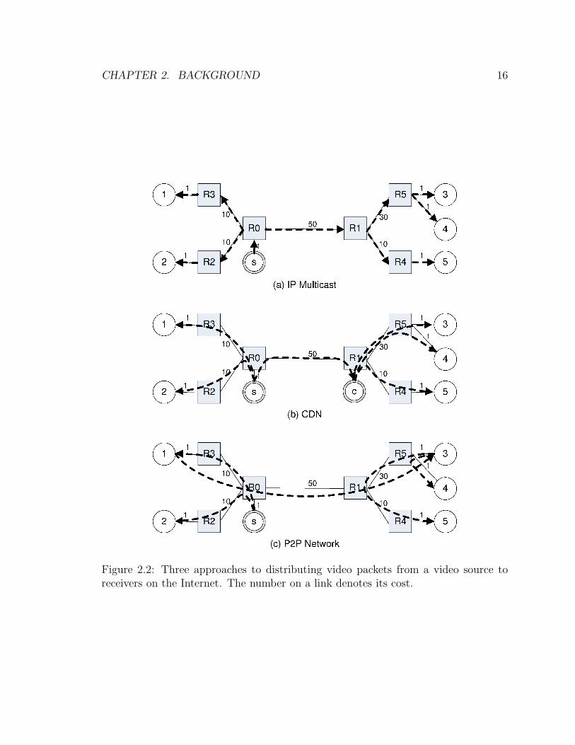
CHAPTER 2. BACKGROUND 16
Figure 2.2: Three approaches to distributing video packets from a video source toreceivers on the Internet. The number on a link denotes its cost.

CHAPTER 2. BACKGROUND 17
serve nearby users, reducing network traffic. The biggest drawback of CDNs is their
high cost. In addition to investing in servers, CDN operators must also pay ISPs
for connecting servers to the Internet. Both costs increase as the number of users
increases.
Researchers began to propose the implementation of the multicast functionality
by hosts at the application layer rather than by routers at the IP layer [12,20] in the
late 1990s. These was in response to the slow and “walled-garden” deployment of
IP multicast a decade after its introduction to the Internet. These early application
layer multicast schemes aimed to replace IP multicast in certain application scenarios,
and like IP multicast, they constructed multicast trees that optimized network cost
function. Inspired by the success of the BitTorrent file sharing application, researchers
began using the swarm technique for live streaming applications that can tolerate tens
of seconds of playback delay [49,86] in 2004. In P2P live streaming applications, each
peer duplicates and forwards packets while at the same time receiving packets from
other peers (see Fig. 2.2c). The most attractive part of P2P networks is their low
cost; only several servers are required for administration purposes, and the upload
bandwidth is contributed by users and increases as the number of users increases.
P2P networks can be used in conjunction with CDNs or IP multicast. For example,
a P2P network may deploy some cache servers to provide upload bandwidth and use
IP multicast inside each “multicast island”.
In small-scale interactive streaming applications, the streaming is either between
two parties, such as in video telephony applications, or can be viewed as a set of
one-to-one connections, such as in video conferencing applications. The use of P2P
networks is not necessary but is attractive in certain situations. For example, many
CHAPTER 2. BACKGROUND 18
users employ a firewall or NAT device and cannot be reached from the outside; they
rely on outside nodes as bridges. Because Internet links are lossy and the losses are
bursty, a sender and a receiver may want to use a set of helper nodes to provide mul-
tiple paths for more reliable communication. In these situations, users can organize
themselves into a P2P network, and peers outside of firewall and NAT devices can
act as bridges or helper nodes.
2.2 Video Coding
The dominant video compression standards are the MPEG series standards [96] pub-
lished by the moving picture experts group (MPEG) of ISO/IEC, whose official des-
ignation is ISO/IEC Joint Technical Committee 1, Subcommittee 29, and the H.260
series standards [95] published by the video coding experts group (VCEG) of ITU-T,
whose official designation is ITU-T Study Group 16, Working Party 3, Question 6.
The two groups often team up to develop standards together. For example, H.262
is equivalent to MPEG-2 Part 2, and H.264 is equivalent to MPEG-4 Part 10, all
developed by the Joint Video Team (JVT). Other popular video coding formats in-
clude WMV from Microsoft, Sorenson from Apple, RealVideo from RealNetworks,
VP8 from Adobe, and the open-source Theora from Xiph.org.
A video stream consists of a series of frames, captured at even time intervals. A
frame is a rectangle of pixels. Each pixel is represented by its RGB values (usually
one byte per value), indicating its red, green, and blue components. For the purpose
of compression, a video frame is divided into slices, a slice is divided into macroblocks,
and a macroblock is divided into blocks.
Video compression exploits the spatial and temporal redundancy of video frames

CHAPTER 2. BACKGROUND 19
and the characteristics of the human visual system. Because the human visual system
is less sensitive to colors than to brightness, the RGB values are converted to YCbCr
values, where Y represents brightness, Cb=B−Y, and Cr=R−Y. The Y component
is sampled for each pixel but the Cb and Cr components are sampled with a lower
resolution. For example, with the 4:2:0 sampling scheme, the Cb and Cr components
are sampled for every 2 × 2 pixels, and hence the 12 bytes of RBG values for four
pixels can be reduced to 6 bytes. Consecutive frames are usually similar (temporal
redundancy), and nearby blocks in a frame are often similar (spatial redundancy).
A video can be compressed by recording these differences rather than the original
signals.
The input frames to the encoder are usually in the CIF/SIF format. The common
intermediate format (CIF) was first introduced in the H.261 standard; the source
input format (SIF) is identical to CIF but is defined in MPEG-1. Colors are encoded
in the YCbCr space. Picture sizes are multiples of macroblocks, which are usually
16×16 pixels. Video telephony and conferencing typically use CIF (352×288 pixels)
or QCIF (176× 144 pixels), while standard TV uses 4CIF (704× 576 pixels). Each
of the Y, Cb, and Cr components are encoded separately.
2.2.1 Block-Based Motion-Compensated Predictive Coding
Most video coding standards use the block-based motion-compensated predictive cod-
ing model shown in Fig. 2.3 [59]. The upper half of Fig. 2.3 shows the encoding pro-
cess. First, the encoder compares an input frame F (n) with reference frames to find
a best match for each macroblock, and records the motion vectors (the motion esti-
mate box in Fig. 2.3). The encoder can use multiple reference frames and the weighted

CHAPTER 2. BACKGROUND 20
Figure 2.3: Block-based motion-compensated predictive encoding and decoding

CHAPTER 2. BACKGROUND 21
sum of the macroblocks of reference frames to find the best match for a macroblock
in F (n). The accuracy of motion vector can be half-pixel or quarter-pixel. Second,
the encoder uses the motion vectors and reference frames to generate a compensated
prediction frame P (the motion compensation box in Fig. 2.3). Third, the encoder
performs discrete cosine transformation (DCT), block by block, on the residual frame
D(n), which is the difference between F (n) and P . The encoder can use a fixed block
size or adapts the block size to the picture characteristics. For example, the encoder
can use a small block size for regions with details and a large block size in regions
without many details. Most values of the coefficient block are zeros, and non-zeros
are concentrated in the top-left corner. Fourth, the resulting coefficient blocks are
quantised (i.e., divided by a scaler to reduce the number of bits to represent each
coefficient) to generate frame X. This is the only step in the encoding process that is
lossy. Fifth, the coefficients are zig-zag scanned, run-length coded, and together with
motion vectors, entropy-encoded to produce the coded bitstream.
The frames P and X are used to generate the reference frame F ′(n). The blocks
of frame X are first scaled and then inversely transformed to generate frame D′(n).
(Frame D(n) and D′(n) differ because the quantisation step is lossy.) Frames D′(n)
and P are added to generate reference frame F ′(n).
The decoding process is similar to the process that generates reference frames.
The decoder first performs the opposite of entropy coding, run-length coding, and
zig-zag scanning to generate frame X, and then uses previously decoded frames and
frame X to generate frame F ′(n).
Frames are divided into I, P, and B frames. The frames between two consecutive
I frames are collectively called a group of pictures (GOP). I frames are encoded
CHAPTER 2. BACKGROUND 22
without motion compensation (intra mode) and can be decoded independently. P
and B frames are encoded with compensation (inter mode). P frames are encoded
using previous frames as reference frames. B frames are encoded with both previous
and later frames as reference frames. Because P and B frames are dependent on I
frames, errors in I frames may propagate into P and B frames. The slices on an
I frame can be divided into I, P, and B slices. I slices are encoded and decoded
independently, P slices are dependent on I slices, and B slices are dependent on I and
P slices. The existence of I slices can prevent an error from propagating to the whole
picture. Note that because of the existence of B frames, the encoding (or decoding)
order is different from the playback order, introducing extra coding delays.
2.2.2 H.264/MPEG-4 AVC
H.264/AVC [95] is the latest video compression standard of the MPEG and H.260
series standards. It defines 17 profiles to support a wide range of applications with var-
ious bandwidths and delays. The main improvements of H.264/AVC, compared with
MPEG-2, are higher compression efficiency and the network abstraction layer (NAL)
for transmission over networks with various delay and loss conditions [73]. H.264/AVC
uses the same block-based, motion-compensated predictive model as its major prede-
cessor, MPEG-2, but achieves significantly higher coding efficiency by incorporating
dozens of improvements. For example, it uses multiple reference pictures, weighted
prediction, variable macroblock size, and quarter-pixel accuracy for motion compen-
sation; it also uses variable block size for DCT. H.264/AVC organizes the coded
bitstream into NAL units. Each NAL unit contains a one-byte header, specifying
the type of the NAL unit. NAL units are classified into two categories: video coding
CHAPTER 2. BACKGROUND 23
layer (VCL) NAL units contain the compressed data (i.e., coefficients and motion
vectors), while non-VCL NAL units contain control information. For example, the
sequence parameter set (SPS) NAL unit carries parameters common to an entire video
sequence, such as the profile and level, the size of video frames, and the maximum
number of reference frames. The picture parameter set (PPS) NAL unit carries pa-
rameters common to a sequence or subset of coded pictures, such as entropy coding
type, number of active reference pictures, and initialization parameters.
H.264/AVC has a number of built-in features for reliable transmission over un-
reliable media. For example, the parameter sets, which are vital for decoding, are
transmitted before the data and can be re-transmitted if lost. H.264/AVC supports
flexible slice size and arbitrary slice order (i.e., the slices of a picture can be coded
in arbitrary order). H.264/AVC also supports slice groups and flexible macroblock
ordering (FMO). Each macro block can be independently assigned to a slice group,
and a slice group can contain one or more slices. H.264/AVC supports slice data
partitions such that different partitions can be transmitted over channels with un-
equal error protection. The coded data that makes up a slice can be placed into
three separate partitions. Partition A contains the slice header and header data for
each macroblock in the slice, partition B contains coded residual data for I slice mac-
roblocks, and partition C contains coded residual data for P and B slice macroblocks.
Partition A is intolerant to errors and is transmitted over the most reliable channels,
while partition B is more tolerant and is transmitted over less reliable channels, and
partition C is the most tolerant and is transmitted over the least reliable channels.

CHAPTER 2. BACKGROUND 24
2.2.3 Multiple Layered Coding
H.264/AVC encodes a video into a single layer. Single layer coding is the most efficient
type of coding, but multiple layer coding is often desired for receiver-side rate-control
and graceful degradation in lossy transmission environments. There are two types of
multiple layer coding: layered coding and multiple description coding (MDC).
In layered coding schemes, a video is encoded into a base layer and one or more
enhancement layers. Higher layers are dependent on lower layers (i.e., a receiver
must have the lower layers to decode higher layers). The more layers a receiver has,
the higher the fidelity of the decoded video is. Scalability can be achieved in three
directions: spatial resolution (reduced picture size), temporal resolution (reduced
frame rate), and quality (signal-to-noise ratio). The most important design criteria
for layered coding schemes is coding efficiency. MPEG-4 Annex G SVC is a layered
coding scheme that extends H.264/AVC. The increase in bit rate of MPEG-4 SVC
relative to H.264/AVC at the same fidelity can be as low as 10% [62].
MDC [25,71] encodes a video into multiple descriptions. Unlike layers in layered
coding, all the descriptions are equal in MDC. A receiver can decode the encoded
video stream using any subset of the descriptions; the fidelity improves when more
descriptions are used. However, MDC has a large coding overhead [19] and is rarely
used in real-world video streaming applications.
2.3 P2P Networks
A P2P network is a distributed system in which a transient population of peers self-
organizes into an overlay network on top of a substrate network to share computing
CHAPTER 2. BACKGROUND 25
power, storage, and communication bandwidth [3]. The substrate network, also called
the underlay network, is usually the Internet.
P2P networks have been used for many applications. P2P file sharing applica-
tions, such as BitTorrent, Gnutella, eDonkey, are among the most popular Internet
applications. The traffic caused by P2P file sharing has been the dominant type of
traffic on the Internet for years. P2P video streaming applications are also popular
among users. PPLive and PPStream, two popular P2P video streaming networks in
China, reported having millions of active daily users as of 2009 [98,99]. Internet tele-
phony is another area where P2P networks have succeeded in the commercial world.
For example, Skype, the most popular Internet telephony service, has tens of millions
of daily active users [100]. Other P2P applications include data storage [32], web
services [47], content publishing [61], etc.
In a P2P network, each peer is both a client and a server. Peers usually have
limited storage and bandwidth, partial knowledge of the neighboring overlay, and
little knowledge of the substrate Internet. Peers may join and leave the P2P network
at any time; the churn of peers poses a great challenge to P2P applications. There
are two basic problems in a P2P network: locating the peers that store a particular
data object given the object’s key or a set of keywords, and retrieving the object
efficiently once knowing which peers have it. Depending on the type of application, a
P2P application also needs to address a number of practical issues, such as incentives
to encourage peers to contribute, issues of fairness among peers to share work load,
accountability and deniability of behavior, and the traffic the application generates
on the substrate Internet.

CHAPTER 2. BACKGROUND 26
2.3.1 Locating and Routing
Being able to locate the peers that have a certain data object is fundamental to any
distributed file sharing and data storage systems. The location problem is sometimes
termed the routing problem because the query for peers that have a certain data object
is routed hop-by-hop to peers who know the answer. In P2P video live streaming
applications, if we consider the video source as an object, the paths that the query
messages traverse from each user to the video source (or the response messages from
the video source to each user) form a multicast tree on the neighboring overlay.
In a P2P file sharing system, data objects are stored distributively at each peer.
Each data object has a unique ID, which is usually obtained by hashing the data
object. Each peer also has a unique ID, which is usually in the same space as the object
IDs. Depending on the mapping of data objects to peers and the organization of peers,
P2P file sharing systems can be classified into structured systems and unstructured
systems.
In a structured system, each data object is stored at a set of peers deterministically
determined by the object ID. Peers are organized in such a way that, if given an
object ID, locating the peers that have the desired object takes a short amount of
time. Without loss of generality, we will assume that object IDs and peer IDs are in
the same m-bit space. Each data object is represented by a key–value pair (K, V ),
where key K is the object ID and value V can be the data object itself or an index
to the object. Each (K, V ) pair is stored at exactly one peer. All the (K, V ) pairs
form a distributed hash table (DHT). The location problem can be stated as: Given
a key K, locate the peer that stores the key-value pair (K, V ).
Table 2.1 summarizes some of the most well-known DHT algorithms. All of the
CHAPTER 2. BACKGROUND 27
algorithms achieve a path length of O(logN) between two arbitrary peers and only
require peers to maintain a routing table of size O(logN), where N is the system
population2. In all of the algorithms, peers statistically equally partition the object
ID space. Each peer “owns” a range of the space and stores a (K, V ) pair, if K
falls in the peer’s range. Given an object ID, all the peers can be ordered by their
“distance” to the object ID. When looking up a key K, each peer routes the query to
the neighbor that is closer to the object ID. Eventually the query will reach the peer
that stores the (K, V ) pair.
The DHT algorithms listed in Table 2.1 differ in the manner that peers partition
the ID space and the definition of distance. Pastry [60] and Tapestry [87] organize the
ID space as a hypercube and form a Plaxton mesh [54] neighboring overlay. Chord [65]
organizes the ID space as a circle modulo 2m, where m is the number of bits in IDs.
Kademlia [45] organizes the ID space as a binary tree and uses the XOR logic to
define distance. Viceroy [43] organizes ID space as a circle of length one and forms
a butterfly-shaped neighboring overlay. CAN [55] centers around a d-dimensional
Cartesian coordinate space on a d-torus and uses Euclidean distance.
Structured systems incur significant overhead when peers join and leave. When a
new peer x joins, peer x needs to acquire its routing table, some peers need to update
their routing tables to include peer x, and some (K, V ) pairs need to be transferred to
peer u. In Chord [65], it takes O(log2N) messages for a new peer to join the system;
in other schemes, the join complexity is O(logN).
In an unstructured P2P file sharing system, the mapping of data objects to peers
is non-deterministic, and the neighboring overlay’s topology is not tightly controlled.
2In CAN, when d = 1
2log2 N , the routing table size is log2 N , and the average path length is
1
2log2 N hops.

CHAPTER 2. BACKGROUND 28
Table 2.1: Comparison of DHT Algorithms
ArchitecturePath
LengthState Size
JoinComplexity
CAN d-dimension torus 14d d√N 2d O(logN)
Chord Circle O(logN) O(logN) O(log2N)
TapestryHypercube and Plaxtonmesh overlay
O(logN) O(logN) O(logN)
PastryHypercube and Plaxtonmesh overlay
O(logN) O(logN) O(logN)
Kademlia Binary tree O(logN) O(logN) O(logN)
Viceroy Circle and butterfly overlay O(logN) O(1) O(logN)
Unstructured systems rely on flooding or random walk to locate the peers that have a
certain data object. The key can can be the unique object ID, or a group of keywords.
A peer floods a query message to all of its neighbors, or to a group of neighbors selected
with a probability function. Each peer compares the key or keywords in the query
message with the data objects it has, and responds accordingly.
Because the queries are flooded, unstructured systems incur large communication
overhead, which limits the scale of P2P applications. To improve scalability, some
unstructured systems, such as Gnutella and Kazaa, divide peers into two categories:
super peers and normal peers. A normal peer attaches to one or several super peers.
A normal peer stores the data objects itself but stores the key–index pair of the data
objects it has at the super peer. If a normal peer wants to look up a data object,
it asks the super peers to do so. Super peers form an unstructured network and use
flooding or random walk to locate the peers that store the requested data objects.
Unstructured systems are suitable for P2P systems with a dynamic population
because the cost of dealing with peer churn is low. A new peer joins the system by
CHAPTER 2. BACKGROUND 29
attaching to some existing peers. When a peer leaves, its neighbors simply delete it
from their routing tables.
2.3.2 Retrieving Data Objects
The retrieval problem arises from downloading large files [92] and is drawing renewed
attention due to growing video streaming applications [27, 37, 64, 88]. To facilitate
large file downloads, Kazaa, eDonkey, and BitTorrent allow a peer to download a data
object in parts from multiple peers. Among these applications, the swarm technique
introduced in BitTorrent is especially efficient.
BitTorrent [14] splits a file into fixed-size chunks, which are in turn divided into
fixed-size pieces. Peers advertise their buffer maps, which describe the chunks they
have, to their neighbors and request missing pieces from their neighbors. BitTorrent
employs the rarest-first strategy to select pieces to request. A peer requests the
missing pieces that are least common in its neighbors’ buffer maps. To avoid a
situation in which many peers are requesting the least common piece at the same
time, the rarest-first strategy includes randomization among at least several of the
least common pieces. BitTorrent employs a tit-for-tat strategy to encourage peers to
contribute upload bandwidth. A peer uploads to the four requesting peers depending
on who has the highest download rate. BitTorrent limits the number of peers to four
because TCP congestion control behaves poorly when sending over many connections
at once. A new peer may have upload bandwidth and wish to share, but typically
has no data to upload to other peers. BitTorrent employs an optimistic unchoking
strategy to address this issue. At any given time there is a single peer that is unchoked
regardless of its upload rate. The peer that is optimistically unchoked rotates every 30
CHAPTER 2. BACKGROUND 30
seconds. Newly connected peers are three times as likely be optimistically unchoked
in the rotation, which gives them a decent chance of getting a complete piece to
upload.
Videos are typically large files but streaming imposes extra constraints. For P2P
on-demand streaming applications, once a peer has started watching a video, the
chunks after the current playback position have deadlines, and the chunks before
the current playback position are useless. A peer may seek new positions during
the playback, which changes the usefulness and urgency of chunks and may leave
some chunks never fetched [84]. For live streaming applications, because of the delay
constraints, each peer only buffers a small segment of the video, which makes the
rarest-first and tit-for-tat strategies less effective than in P2P file sharing applications.
2.4 P2P Live Streaming
A large number of P2P video live streaming schemes have been proposed in the
past two decades. These schemes pursue various directions and sometimes integrate
techniques used in other schemes to form various hybrid schemes. As a consequence,
P2P video live streaming schemes can be classified using various perspectives. In this
section, we briefly introduce the classifications and representative schemes.
2.4.1 Classification
Depending on whether or not explicit trees exist, P2P video live streaming schemes
can be classified into tree-based and swarm-based schemes. In tree-based schemes,
peers form parent–child relationships. Upon receiving a packet, a peer immediately
CHAPTER 2. BACKGROUND 31
pushes the packet to its children. Therefore, tree-based schemes are sometimes called
tree-push schemes or simply push schemes. Swarm-based schemes are sometimes
called treeless schemes or mesh-based schemes. In swarm-based schemes, the video
is sequentially split into chunks of fixed sizes (in bytes or in seconds). Peers form
neighboring relationships and advertise their bit-maps, which describe the chunks
they have to neighbors, and exchange missing chunks.3
According to the number of trees, tree-based P2P video live streaming schemes can
be classified into single or multiple tree-based schemes. In single tree-based schemes,
the video is encoded into a single layer and peers construct a single tree that all
the packets follow. In multiple trees-based schemes, the video is either encoded
into a single layer but interleaved into multiple substreams or encoded into multiple
layers with MDC or LC. Peers construct a separate tree for each substream. Single
tree-based schemes have lower overhead. Multiple trees-based schemes utilize peers’
upload capacity more efficiently—a peer can be a leaf node on one tree but upload
to other peers on a different tree. Multiple trees may be interior node-disjoint (i.e., a
peer can be an interior node on at most one tree) or have common interior nodes.
According to whether peers first construct a mesh neighboring overlay, P2P video
live streaming schemes can be classified into mesh-first or tree-first schemes. In mesh-
first schemes, each peer maintains relations with a number of peers (called neighbors).
These relationships form the edges of the neighboring overlay. Then peers build a
spanning tree on the neighboring overlay. In tree-first schemes, there is no neighboring
3In this thesis, we do not use the terms treeless, mesh-based, push, or tree-push to describe ascheme in order to avoid possible confusion. For example, tree-based schemes may first constructa mesh neighboring overlay, swarm-based schemes may use the push mode, and the term push hasdifferent meanings in swarm-push and tree-push. The terms swarm-based, swarm-pull, and swarm-
push in this survey have the same meaning as mesh-based, mesh-pull, and mesh-push in [38], anddata-driven has the same meaning as in [37].
CHAPTER 2. BACKGROUND 32
Figure 2.4: (a) Source tree. (b) Bi-directional shared tree. (c) Uni-directional sharedtree.
overlay and the tree is built in one step.
If an application allows multiple video sources, it needs to construct a separate
source tree for each video source, or construct a shared tree. On a source tree, the
video source is the tree root and tree edges are uni-directional (see Fig. 2.4a). There
are two types of shared trees. The first type, as shown in Fig. 2.4b, makes all tree
edges bi-directional; each node forwards packets to its parent and children except the
one that the packets come from. With the second type, as shown in Fig. 2.4c, video
packets are forwarded from the video source first to the tree root and then to all the
nodes.
In a recent work [85], we propose to classify P2P live streaming schemes according
to the algorithmic choices to their designs. To achieve the basic objective of distribut-
ing video packets from the video source to peers, a scheme needs to fulfill three tasks:
(1) to determine the supplier-receiver relationships4 between peers for each packet
such that the supplier–receiver relationships collectively form a tree that reaches all
the peers (i.e., no loops, no partitions, and each node has an in-degree of one); (2) if
a supplier–receiver relationship applies to more than one packet, a scheme must deal
4The terms supplier and receiver are equivalent to the terms parent and child in the context oftree-based schemes. We use the terms supplier and receiver in the context of both tree-based andswarm-based schemes, and use the terms parent and child only in the context of tree-based schemes.

CHAPTER 2. BACKGROUND 33
Figure 2.5: Taxonomy with respect to tree-building algorithms
with the situation when the supplier or receiver leaves before all the packets are sent;
and (3) to handle lost packets. Fig. 2.5 summarizes the algorithmic choices to the
design of P2P live streaming schemes. In the following we will discuss the first task;
we will discuss the second and third tasks in Section 2.6.
There are three basic algorithmic choices to determine the supplier–receiver rela-
tionships. The first choice is to use a central server to compute the supplier–receiver
relationships using a centralized algorithm and to inform each peer. The supplier–
receiver relationships should apply to the whole stream (i.e., tree-based). It is possible
that the server computes the supplier–receiver relationships for each chunk separately,
but this carries no benefit and the server’s workload and communication overhead
would be too large. The centralized method can be explicitly or implicitly mesh-first.
In the latter case, peers do not have neighbors but the central server implicitly main-
tains a mesh neighboring graph. For example, if the central server maintains each
peer’s virtual network position, it can implicitly construct a complete neighboring
graph.
CHAPTER 2. BACKGROUND 34
The second choice is to use a recursive algorithm. Each peer i first requests
the video source to be the supplier. The video source either accepts the request or
delegates to another peer. This process repeats until peer i is accepted by some peer.
A peer accepts receivers only if it has spare upload capacity. The recursive method
is tree-first. As long as a peer only delegates to its receivers, the recursive method
guarantees building a tree that reaches all the peers. Same as the centralized method,
the supplier-receiver relationships should apply to the whole stream. We remark that
recursive algorithms are distributed, but not fully distributed—peers close to the
video source have high workload. We use the term recursive to differentiate them
from fully distributed algorithms.
The third choice is to use a fully distributed algorithm. Most fully distributed
schemes are mesh-first. Peers must maintain sufficient neighbors such that the neigh-
boring graph remains connected in the presence of peer churn. In a dynamic envi-
ronment, flooding each received video packet to all the neighbors can guarantee the
packet reaching all of the peers. However, flooding also results in a large amount of
unnecessary traffic because multiple copies of the video packet are sent to peers. To
reduce traffic, peers can advertise5 other information with a small size to neighbors
such that peers can arrange the transmission of video packets using this information.
There are two possible choices to achieve this: swarming and routing.
In the swarming method, each chunk is uniquely numbered, each peer advertises
its bit-maps—each bit in the bit-map indicates whether the peer has a chunk—to
neighbors, and peers establish the supplier–receiver relationship for each chunk. The
establishment of a supplier–receiver relationship may be initiated by the receiver or
5Flooding refers to the practice where a peer forwards each received packet to all the neighborsexcept the neighbor from which the packet comes. Advertising refers to the practice where a peerforwards packets generated by itself to all its neighbors.
CHAPTER 2. BACKGROUND 35
the supplier (called the pull and push mode of the swarm-based scheme in [7]). When
initiated by the receiver, the receiver requests one, and only one, copy of each chunk
from a selected neighbor, and hence it will not receive duplicated chunks. When
initiated by the supplier, the supplier pushes chunks to neighbors that the neighbors
do not already have. However, because a peer’s local copy of a neighbor’s bit-map
may be stale, peers may receive duplicated chunks. Note that with the swarming
method, peers establish supplier–receiver relationships for a chunk after knowing
whether neighbors have the chunk; with other methods, a priori knowledge is not
required. Because the establishment of supplier–receiver relationships are based on
data availability, the swarming method is said to be “data-driven” [37, 86]. In the
routing method, each peer advertises routing information to neighbors periodically
and establishes the supplier–receiver relationship for the whole stream. The establish-
ment of supplier–receiver relationships is always initiated by the receiver. The routing
information a peer advertises may be network-related (called network-driven routing),
such as the peer’s geographic location (e.g., geographic routing), the peer’s ID (e.g.,
DHTs), the peer’s hop counts to the video source (e.g., distance-vector routing), and
the costs between peers (e.g., link-state routing). There are well-known algorithms to
build spanning trees on the neighboring graph with these information. The routing
information a peer advertises may also be data-related (called data-driven routing),
such as the peer’s bit-maps or the sequence number of the most recent packet the peer
has. Although several data-driven routing schemes exist, it is not fully understood
which algorithms can guarantee building a spanning tree (i.e., no partitions, no loops,
and no duplicated packets) on the neighboring graph and what properties the tree
will have.

CHAPTER 2. BACKGROUND 36
Since peers have limited upload capacity, both the swarming method and the
routing method (including centralized and fully-distributed) need to guarantee that
a peer’s workload is within its upload capacity. For the routing method where the
supplier–receiver relationships apply to the whole stream, this problem is typically
addressed by limiting the number of receivers for each supplier. For the swarming
method where the supplier–receiver relationships apply to chunks, this problem can
be addressed by limiting the output queue length of the supplier.
In mesh-first schemes, peers usually first maintain a membership table and then
select neighbors from the table. Unlike with neighbors, a peer does not periodically
exchange information with peers in its membership table. A peer can obtain its
membership table using a centralized method (i.e., a new peer asks a tracker for
peers already in the system), or a recursively method (i.e., a peer uses a recursive
process to find peers in the system), or a fully distributed method (i.e., a new peer
knows at least one peer already in the system and uses it to find other peers in the
system)6. The use of a membership table can reduce the time required for a peer
to find new neighbors and can also reduce the tracker’s workload. The neighboring
graph can be structured (i.e., organized with DHTs) or unstructured. It can also
“mirror” the substrate Internet such that the paths between peers will have lower
costs.
6We classify P2P video live streaming schemes according to tree-building algorithms, not themethod that a peer uses to obtain its membership table.
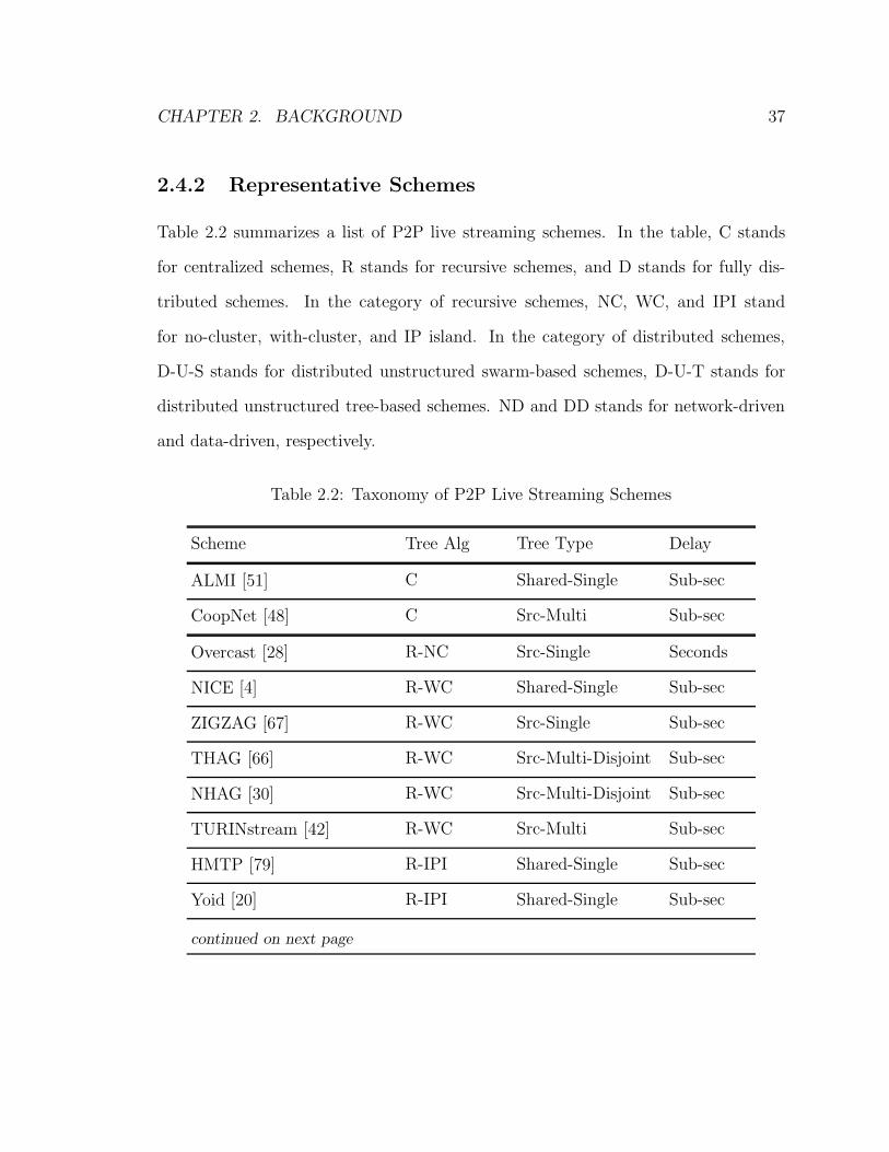
CHAPTER 2. BACKGROUND 37
2.4.2 Representative Schemes
Table 2.2 summarizes a list of P2P live streaming schemes. In the table, C stands
for centralized schemes, R stands for recursive schemes, and D stands for fully dis-
tributed schemes. In the category of recursive schemes, NC, WC, and IPI stand
for no-cluster, with-cluster, and IP island. In the category of distributed schemes,
D-U-S stands for distributed unstructured swarm-based schemes, D-U-T stands for
distributed unstructured tree-based schemes. ND and DD stands for network-driven
and data-driven, respectively.
Table 2.2: Taxonomy of P2P Live Streaming Schemes
Scheme Tree Alg Tree Type Delay
ALMI [51] C Shared-Single Sub-sec
CoopNet [48] C Src-Multi Sub-sec
Overcast [28] R-NC Src-Single Seconds
NICE [4] R-WC Shared-Single Sub-sec
ZIGZAG [67] R-WC Src-Single Sub-sec
THAG [66] R-WC Src-Multi-Disjoint Sub-sec
NHAG [30] R-WC Src-Multi-Disjoint Sub-sec
TURINstream [42] R-WC Src-Multi Sub-sec
HMTP [79] R-IPI Shared-Single Sub-sec
Yoid [20] R-IPI Shared-Single Sub-sec
continued on next page

CHAPTER 2. BACKGROUND 38
continued from previous page
Scheme Tree Alg Tree Type Delay
Island multicast [29] N/A Src-Single Sub-sec
CAN-based [56] D-DHT Src-Single Sub-sec
Bayeux [90] D-DHT Src-Single Sub-sec
SplitStream [8] D-DHT Src-Multi-Disjoint Sub-sec
Borg [82] D-DHT Src-Single Sub-sec
Chainsaw [49] D-U-S-Pull Src-Chunk Minutes
CoolStreaming [86] D-U-S-Pull Src-Chunk Minutes
Prime [41] D-U-S-Pull Src-Chunk Minutes
Pulse [52] D-U-S-Pull Src-Chunk Minutes
LayerP2P [40] D-U-S-Pull Src-Chunk Minutes
R2 [70] D-U-S-Push Src-Chunk Seconds
CoolStreaming+ [75] D-U-T-DD Src-Multi Seconds
SPANC [9] D-U-T-DD Src-Multi Seconds
GridMedia [81] D-U-T-DD Src-Multi Seconds
Substream Trading [39] D-U-T-DD Src-Multi Seconds
Narada [12] D-U-T-ND Src-Single Sub-sec
Gossamer [10] D-U-T-ND Src-Single Sub-sec
TreeClimber [83] D-U-T-ND Src-Single Seconds
OMNI [5] D-U-T-ND Src-Single Sub-sec
FastMesh [58] D-U-T-ND Src-Multi Seconds
ChunkySpread [68] D-U-T-ND Src-Multi Seconds
continued on next page

CHAPTER 2. BACKGROUND 39
continued from previous page
Scheme Tree Alg Tree Type Delay
Treebone [69] D-U-T-ND Src-Single Seconds
Narada/ESM [12] targets small group multicast applications with multiple sources.
First, the protocol, called Narada, constructs a mesh neighboring overlay G that mir-
rors the substrate Internet. Each peer periodically measures its delay to every other
peer and adds or drops edges on G according to the utility gain or loss, which are
defined in terms of the number of peers to whom the delays via overlay edges become
less or more and by the extent of changes. Then peers run a BGP-like protocol to
maintain a unicast routing table. Because peers’ out-degrees on the multicast tree are
bounded by their upload bandwidth, Narada uses a variant of the shortest widest path
algorithm. Similar to BGP, each routing entry contains a list of peers on the path to
the destination in order to prevent forwarding loops. Finally, peers construct a source
tree on G using RPF for each source. Narada achieves high substrate utilization at
the expense of scalability. Each peer needs to monitor the delays from itself to every
other peer to optimize the overlay G.
Chainsaw [49] is a proof-of-concept implementation of the swarm-pull scheme.
Each peer connects to a set of randomly selected neighbors to form a neighboring
overlay (each peer has 30–40 neighbors). Peers employ the “random chunk, random
peer” scheduling algorithm and notify their neighbors immediately upon receiving
a new packet (30-40 messages are generated for each received packet). Each peer
maintains a window-of-interest, which is the set of sequence numbers of packets that
the peer is interested in acquiring, and a windows-of-availability, which is the set of
sequence numbers of packets that the peer already has. A peer randomly selects a
CHAPTER 2. BACKGROUND 40
packet in its window-of-interest, and pulls it from a randomly selected neighbor. A
peer limits the number of outstanding requests to a neighbor to balance the workload
of its neighbors. A problem with the random chunk algorithm is that some chunks
are never requested from the source and hence are lost at all the peers. To fix this
problem, the source records the chunks it has uploaded. When a peer requests a
chunk that has been uploaded, the source will send the oldest chunk that has never
been uploaded rather than the requested chunk.
CoolStreaming is one of the few schemes that have been deployed on the Inter-
net. The original version [86] uses a swarm-pull scheme; the new version [75] changes
to a tree-push scheme. The original CoolStreaming constructs a random neighboring
overlay using the scalable probabilistic membership protocol (SCAMP) [22]. SCAMP
is a fully distributed membership management protocol in which each peer maintains
a random subset of size O(logN) of the population. A peer randomly selects a fixed
number of peers in its membership table to neighbor with. The authors tried differ-
ent peer degrees on the neighboring overlay and have concluded that 4 is reasonably
good. The packet loss rate decreases marginally for higher degrees. A peer updates
its neighbor list periodically or when triggered by the departure of an existing neigh-
bor. In a periodic update, the peer replaces the neighbor that has the least amount of
incoming and outgoing traffic between itself and the peer. The use of a membership
table reduces the number of times needed to contact the tracker and helps a peer to
find a new neighbor faster. However, the benefit of using a membership management
protocol such as SCAMP instead of using a naive approach to construct a random
neighboring overlay is not justified, so the new version changes to a naive approach.
CHAPTER 2. BACKGROUND 41
A video is split into one second chunks. Each peer has a sliding window of 120
chunks. Every second, a peer advertises its buffer map to its neighbors and pulls
missing chunks from its neighbors. The scheduling algorithm mixes chunk and neigh-
bor selection together. A peer first considers chunks available from one neighbor,
two neighbors, etc. in sequential order. If a chunk is available from more than one
neighbor, the neighbor with the highest bandwidth and from which the estimated
chunk arrival time falls before the deadline is selected. The authors evaluate the
scheme with a 500 kb/s video streaming rate and about 200 hosts on PlanetLab [97].
A peer buffers 10 seconds of video before playing it back. For the nodes that have an
ON/OFF period of more than 400 seconds, 95-97% of the chunks arrive in time; for
stable nodes, 97-98% of chunks arrive in time. The overhead for exchanging buffer
maps is about 2%.
In the new CoolStreaming [75], the neighboring overlay construction is simpli-
fied. A new peer x contacts a well-known RP for its membership table of size M , from
which it selects neighbors randomly. Peer x exchanges its membership table with a
neighbor only once, immediately after establishing the neighboring relation. When a
neighbor becomes unavailable, peer x deletes the neighbor from its membership table
but will not flood the information.
The video is split into chunks of equal size and interleaved into S substreams.
Neighbors periodically exchange buffer maps. The buffer map peer x sends to peer y
consists of two parts: an S-tuple of sequence numbers of the most recently received
chunks for every substream, and an S-tuple indicating which substreams peer x sub-
scribes to peer y. A peer always accepts subscription requests from its neighbors
CHAPTER 2. BACKGROUND 42
until it has M children. If a parent does not have enough upload capacity, its chil-
dren compete for the upload capacity. A parent will not voluntarily drop a child; it
is up to the child to decide whether to switch parents. A peer tries to ensure that all
the substreams it receives advance at a similar pace, and its parent for a substream
proceeds at a similar pace as its neighbors. A peer monitors its parents for two upper
bounds: the upper bound of acceptable deviation between substreams, and the upper
bound of acceptable deviation between a parent and other neighbors. If they are not
satisfied, the peer will start looking for a new parent.
SPANC [9] aims to minimize the packet delivery delay. It uses an existing
neighboring overlay construction scheme. The video is split into chunks of t seconds
and interleaved into S substreams. Each packet has a sequence number and each peer
periodically advertises its most recent packet’s sequence number in each substream
to neighbors. A new peer x is assigned a set of potential parents, and each parent
reserves a certain amount of bandwidth for peer x. Given the most recent packets’
sequence numbers of potential parents in each substream and the delivery delay d(y, k)
from the source to peer x if peer y is the parent in substream k, peer x calculates
a “schedule” that minimizes∑Sk=1 d(pk, k), where pk is peer x’s parent in substream
k. After every interval of length T , peer x calculates a new schedule if its network
conditions have changed (e.g., departure of parents or change of packet loss rate).
Unlike most other schemes, SPANC considers lossy Internet links and uses network
coding for loss recovery. For each chunk of i original packets, j extra NC packets,
which are linear combination of the original packets, are generated by parents of peer
x. Peer x can reproduce the i original packets if it receives any i packets out of the
i+j packets. Every interval of length t, peer x calculates the value j as the sum of the

CHAPTER 2. BACKGROUND 43
exponential moving average and variance of the number of lost packets in previous
chunks. Peer x then assigns the j NC packets to parents in such a way that minimizes
the worst-case delay among all parents.
GridMedia [81] splits the video into S substreams and uses packet-sized chunks.
A new peer contacts a well-known RP for its initial membership table, and exchanges
membership tables with neighbors periodically. A peer selects some neighbors that
have the shortest RTT and selects other neighbors randomly. This effort aims to
mirror the overlay to the substrate while retaining the favorable property of random
graphs. However, because the membership table is small compared with the popu-
lation, the probability of choosing nearby neighbors is low. Neighbors periodically
exchange keep-alive messages; a departing peer notifies its neighbors and the message
is flooded within a limited number of hops. Each peer keeps track of the data packets
sent to and received from neighbors, and drops a neighbor if the volume is below a
certain level.
The pull mechanism is similar to the original CoolStreaming [86]. The pull mech-
anism is used in the start-up phase when trees do not exist and also as a loss re-
covery mechanism. GridMedia requires that peers have synchronous clocks; every
peer synchronizes with RP when joining the system. At the end of every subscribing-
pushing-packets-interval, a peer x requests substreams from neighbors, which pushes
packets of the subscribed substreams to peer x during the next interval. Peer x uses
the roulette wheel selection algorithm to select parents for each substream; it selects
a neighbor y to be the parent with a probability proportional to the percentage of
packets it has received from peer y during the last interval. Peer x pulls the remaining
packets and the lost packets from neighbors; it uses the same roulette wheel selection

CHAPTER 2. BACKGROUND 44
algorithm to select the neighbors to pull from.
2.5 Traffic Locality in P2P Video Streaming Ap-
plications
The enormous traffic of P2P video streaming applications causes ISPs great financial
expenditure and threatens the quality of other Internet services. To avoid unpleasant
traffic throttling or blocking, P2P video streaming applications need to address ISPs’
concerns, i.e., to reduce inter- and intra-AS traffic on the Internet.
The Internet traffic generated by a P2P streaming application is the product of
the amount of packets that need to be transmitted and the costs of the paths these
packets take. The amount of packets can be reduced by using coding schemes—
including source coding and channel coding schemes—with less overhead. The cost
of a path is best measured by its IP routing cost. This is because the routing costs
of Internet links are configured by ISPs and reflect the costs of carrying packets on
these links from the ISPs’ perspective. The cost information of Internet links may be
provided by ISPs directly, as proposed in [1, 74], or be inferred by P2P applications.
In the latter case, the propagation delay of an Internet link is typically used as an
alternative to its IP routing cost because the two parameters are highly correlated.
In interactive streaming applications that use helper peers to provide multiple
paths or to traverse NATs, helper peers are usually selected to be in the “middle”
of a sender and a receiver, and network traffic is mainly determined by the coding
overhead. In large-scale P2P live streaming applications, network traffic is deter-
mined by both the coding overhead and the propagation paths of packets. P2P live
CHAPTER 2. BACKGROUND 45
streaming applications typically use highly efficient video coding standards and do
not use channel coding. In the following, we focus on packets’ propagation paths in
large-scale P2P live streaming applications.
2.5.1 Finding the Minimum Cost Tree
In a large-scale P2P live streaming application, given a video source and a number of
receivers, from the perspective of the IP layer, the propagation tree with the minimum
cost is a Steiner tree. The substrate Internet can be considered as a sparse graph
where the routers and peers are nodes and Internet links are edges. The Steiner tree
roots at the video source and spans all the peers. All the leaf nodes of the Steiner
tree are peers and all the inner nodes are routers. The Steiner tree problem is NP-
hard. IP multicast protocols use the shortest path tree (SPT) algorithm. There are
several IP multicast protocols, such as PIM, the multicast open shortest path forward-
ing (MOSPF) protocol, and the distance-vector multicast routing protocol (DVMRP).
DVMRP is the multicast counterpart of the unicast RIP and uses a distance-vector
algorithm. MOSPF is the multicast counterpart of the unicast OSPF and uses a
link-state algorithm. PIM relies on unicast routing protocols. The multicast tree is
formed by the collective IP unicast paths from the video source to each receiver. IP
multicast trees are typically used as the benchmark to evaluate how efficiently P2P
live streaming applications can utilize the Internet.
From the perspective of application layer, the propagation tree with the minimum
cost is a minimum spanning tree (MST) of the neighboring overlay graph where the
nodes are peers and the edges are IP unicast paths between peers that are reachable
(i.e., not behind firewall and NAT devices). The MST of a graph can be built using
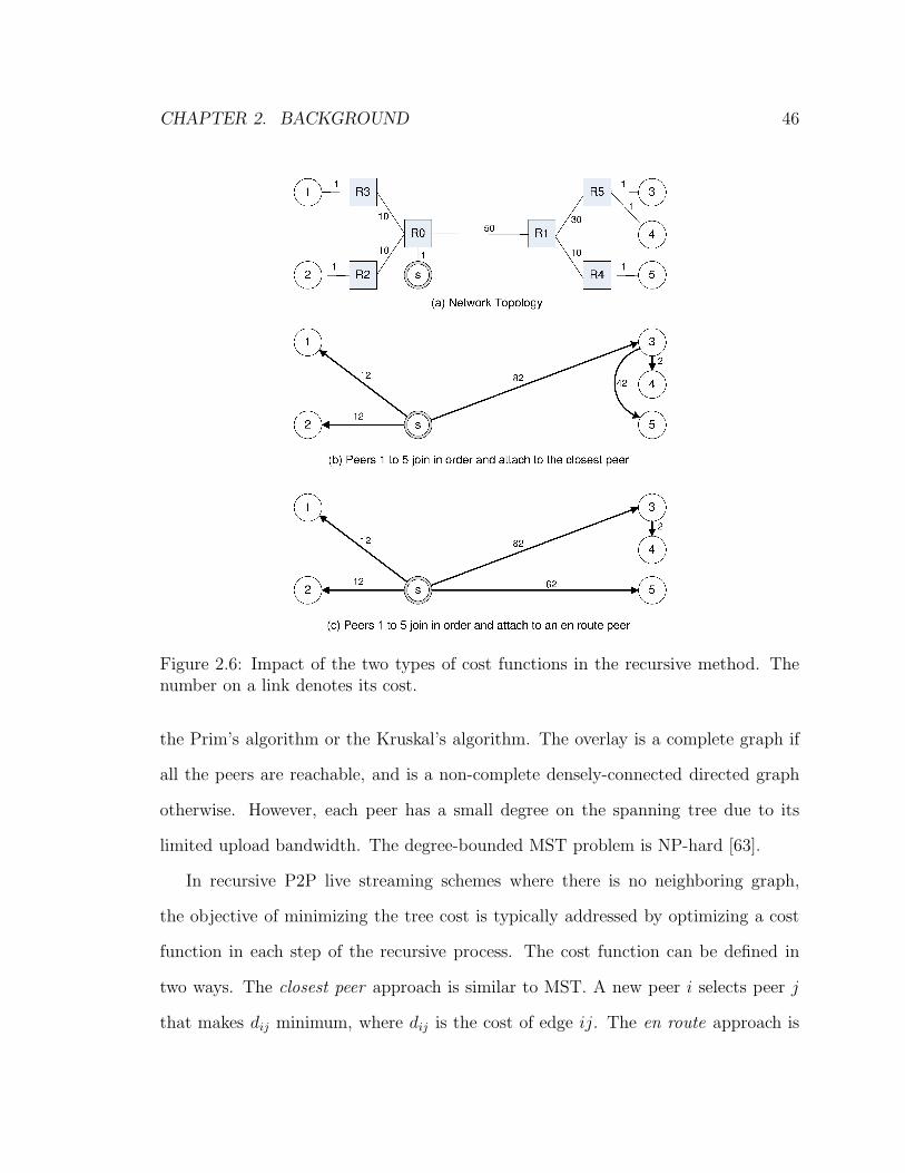
CHAPTER 2. BACKGROUND 46
Figure 2.6: Impact of the two types of cost functions in the recursive method. Thenumber on a link denotes its cost.
the Prim’s algorithm or the Kruskal’s algorithm. The overlay is a complete graph if
all the peers are reachable, and is a non-complete densely-connected directed graph
otherwise. However, each peer has a small degree on the spanning tree due to its
limited upload bandwidth. The degree-bounded MST problem is NP-hard [63].
In recursive P2P live streaming schemes where there is no neighboring graph,
the objective of minimizing the tree cost is typically addressed by optimizing a cost
function in each step of the recursive process. The cost function can be defined in
two ways. The closest peer approach is similar to MST. A new peer i selects peer j
that makes dij minimum, where dij is the cost of edge ij. The en route approach is

CHAPTER 2. BACKGROUND 47
similar to SPT. Peer i selects peer j that makes dij + djs minimum, where s is the
video source. Fig. 2.6b and 2.6c illustrate the trees built with the two approaches.
In mesh-first P2P live streaming schemes, including fully-distributed and cen-
tralized schemes, traffic locality is addressed when selecting peers as neighbors and
when selecting neighbors to exchange video packets. In existing large-scale P2P live
streaming deployments, a peer does not consider other peers’ locations on the sub-
strate Internet in the two selections, and hence enormous Internet traffic ensues [2].
Several studies [1, 11, 74] on P2P file sharing applications propose that peers only
neighbor with “nearby” peers (with respect to their locations on the substrate In-
ternet) to construct the neighboring overlay in order to reduce cross-AS traffic and
report positive results. However, compared to file sharing applications, live streaming
applications have more rigid delay constraints. Whether this strategy is applicable
to P2P live streaming applications remains an open question in the literature. On
the neighboring overlay graph, two types of low-cost trees are often built: MST and
SPT. However, when peers’ out-degrees on the tree are bounded, both problems are
NP-hard.
When the propagation tree is optimum according to a cost function, the arrival
of a new peer may cause existing peers to change their parents to make the new tree
optimum. In the centralized method, the central server periodically computes the
optimum tree and instructs peers to switch parents. In the fully distributed tree-
based method, peers periodically check whether to switch parents. In the recursive
method, peers periodically re-join the tree.
CHAPTER 2. BACKGROUND 48
2.5.2 Finding Nearby Peers
Network traffic can be greatly reduced if peers can select nearby peers as neighbors
and select nearby neighbors to exchange packets or chunks. The easiest way for a peer
to find nearby peers is to use an ISP-supported oracle service, as proposed in [1]. This
oracle service ranks peers according to their proximity to a requesting peer. In the
same spirit, the P4P architecture [74] provides an interface for the substrate Internet
to communicate cost information to P2P applications. Alternatively, peers can infer
the distance to another peer without the help of ISPs. In [11], peers use a CDN’s
redirecting information, and in [31], peers uses the BGP prefixes.
The most commonly used method to find nearby peers is to use a network po-
sitioning scheme. The basic idea of network positioning is to model the Internet as
a D-dimensional space. Each host has a coordinate in the D-dimensional space and
the distance between two hosts can be estimated from their network coordinates.
Network positioning schemes greatly reduce the probing overhead since a peer only
measures the RTTs to a small number of other hosts. There are two types of network
positioning schemes: centralized and distributed.
The global network positioning system (GNS) [46] is a typical centralized scheme.
First, a small set of M landmark hosts measure the RTTs, and the results are used
as the distance metric between one another, producing a M ×M matrix. Then the
coordinates of these landmarks in a D-dimensional space are computed such that
the difference between the measured distance and the calculated distance in the D-
dimensional space is minimized. An ordinary host can measure the distances to these
landmarks and calculate its own network coordinate. Because the landmark hosts are
used by all of the peers, they may become bottlenecked.

CHAPTER 2. BACKGROUND 49
Vivaldi [15] is a distributed network positioning system. Vivaldi uses a simple
distributed algorithm to reduce the estimation errors caused by the triangular in-
equity (i.e., the RTT between nodes x and y is greater than the sum of the RTT
between nodes x and z and the RTT between nodes z and y) of the Internet. Vivaldi
minimises the sum of squared errors between measured RTTs and computed RTTs
by analogizing the triangular inequity to the displacement in a physical mass-spring
system. Thus, minimizing the energy in a spring network is equivalent to minimizing
the squared-error.
2.6 Reliability in P2P Video Streaming Applica-
tions
In P2P video streaming applications, packet loss at a receiver is caused either by
the sender failing to send packets in time (e.g., the sender has left or is experiencing
congestion) or by errors of the Internet link between the sender and the receiver.
Sender-related packet loss is typically bursty. In line with the end-to-end principle,
the Internet only provides the best-effort delivery of IP packets. Studies [50,76] show
that a packet loss rate of several percent is not rare on Internet links; they also show
that packet loss often occurs in bursts of consecutive loss.
In interactive streaming applications that use helper peers, a sender and a receiver
typically use only one intermediate peer for each path. When a helper peer leaves,
the sender and receiver find another helper peer. In tree-based P2P live streaming
applications, all the peers form a tree. When a peer leaves, all the children need to
find another parent. We call this process tree-repairing. Fast tree-repairing is critical

CHAPTER 2. BACKGROUND 50
to the playback smoothness in P2P live streaming applications because when a peer
leaves, all of its descendants may be impacted.
In the following, we first discuss the error correction techniques in live streaming
and interactive streaming applications and then discuss fast tree-repairing techniques
in live streaming applications. The discussion also addresses the second and third
tasks in Section 2.4.
2.6.1 Error-Correction
There are two choices to correct or conceal packet loss: coding and re-transmission.
The coding method can be used for applications that only tolerate a delay of several
hundred milliseconds, but it has a larger overhead and performs poorly when errors
occur in consecutive bursts. The re-transmission method has little overhead but
introduces several seconds of delay.
In P2P live streaming applications, both the re-transmission and coding methods
can be used, but the former is preferred. There are three choices for re-transmission.
First, a peer can request its supplier to send a missing packet if it is in a supplier-
receiver relationship. (We call this method point-to-point re-transmission.) With
this method, if a packet is lost at a peer, the packet will be lost at all the peer’s
descendants. Second, a peer can request the video source to send a missing packet.
This method requires that the video source has sufficient upload capacity. Third, a
peer can request a neighbor to send a missing packet. (We call this method multi-
point re-transmission.) This method is most effective, but is feasible only if a peer
has neighbors (i.e., explicitly mesh-first) and knows which neighbors have the missing
packets. The latter requirement can be met if peers advertise bit-maps.

CHAPTER 2. BACKGROUND 51
For interactive video streaming applications, lost packets can only be recovered (or
concealed) by the use of a coding scheme. The coding can be done at the source (i.e.,
video coding) or at the channel. We have introduced source coding in Section 2.2,
so we only discuss channel coding in the following. There are many types of channel
coding schemes. On the Internet, a receiver knows whether an IP packet is corrupt
and discards the corrupted packet, and hence erasure code is used. (The corrupted
packets are erased.) Reed Solomon code is the most widely used channel coding
scheme on the Internet. Reed Solomon code can be systematic and non-systematic.
Codes that include the original packets in the output are systematic and codes that do
not are non-systematic. A systematic Reed Solomon code RS(n, k) works as follows.
A sender appends n − k FEC packets to k original packets to form an FEC block
and sends it to the receiver. The receiver can reproduce the original k packets if it
receives any subset of k packets out of the n packets in an FEC block. If the receiver
receives k′ < k of the k original packets and less than k−k′ FEC packets, then k−k′
original packets are lost. Note that the loss of original and FEC packets has different
impacts on the post-FEC loss ratio when more than n− k packets of an FEC block
are lost. For example, for RS(10, 9), if 2 original packets of an FEC block are lost,
the post-FEC loss ratio is 29; if 1 original packet and 1 FEC packet are lost, the post-
FEC loss ratio is 19. The main disadvantages of using FEC are the coding overhead
and coding delay. For interactive streaming applications, FEC should not introduce
a coding delay of more than several hundred milliseconds. Therefore, the FEC block
size n should be a small number.

CHAPTER 2. BACKGROUND 52
2.6.2 Fast Tree-Repairing
In P2P live streaming applications, to reduce packet loss caused by the sender, a
receiver needs to quickly detect the failure of the sender and request another peer to
send the video packets. This is especially important in tree-based schemes. When
a peer leaves, its children or parent need to quickly detect the peer’s departure. A
peer can detect the departure of the sender by using the periodic heart-beat (i.e.,
keep-alive) mechanism. A receiver can also detect the departure of the sender by
monitoring the packet arrivals from the sender.
When the receiver leaves, if the supplier-receiver relationship applies to a chunk
(i.e., in swarm-based schemes), it does not matter whether the supplier continues
to send the remaining packets or not. However, if the supplier–receiver relationship
applies to the whole stream (i.e., in tree-based schemes), the supplier should stop
sending the packets as soon as possible. This means that the supplier–receiver re-
lationships must be renewed periodically. The statement that “the supplier–receiver
relationship applies to the whole stream” should be more accurately expressed as “the
supplier–receiver relationship applies to a segment of length Trn”, where Trn is the
interval between renewals7. Typically Trn is one or two orders of magnitude larger
than a chunk.
When the supplier leaves, if the supplier–receiver relationship applies a video
segment, a receiver needs to first recover lost packets then find a new supplier for
the remaining packets. In the centralized method, the receiver requests the central
server for a new supplier. In the recursive method, the receiver contacts the video
7The interval Trn can be in unit of time or in unit of packets since P2P live streaming applicationshave a near-constant playback rate. Because peers are in approximate synchronicity, when a peerswitches parents, it is better to specify from which packet the parent–child relationship applies.
CHAPTER 2. BACKGROUND 53
source and repeats the recursive process. In the fully distributed routing method, the
receiver relies on the routing algorithm. However, in a recursive or fully distributed
scheme, repairing the tree in such a manner takes a long time.
A fast tree-repairing (FTR) mechanism can greatly reduce the time that an or-
phaned peer takes to find a new parent. When its parent leaves, a peer immediately
attaches to a temporary parent. Because FTR may cause forwarding loops and cause
the tree no longer optimized if a scheme also aims to minimize the propagation tree
cost, the peer needs to look for a new parent using the recursive process or using
the distributed routing protocol and switches to that parent. (A new peer can join
the system in a similar manner.) If the supplier–receiver relationship applies to a
chunk, the receiver can ignore tree-repairing and rely on the error control mechanism
to recover the chunk.
Because peers have limited upload bandwidth, the fast tree-repairing mechanism
also needs to manage peers’ workload. There are two methods for managing workload.
When a peer receives a request to be a parent, it may employ a connection admission
control (CAC) mechanism, i.e., it grants the request if it has spare upload bandwidth
and rejects the request otherwise. Another method is to accept the requests, and let
children compete for upload bandwidth until some children decide to back off.
2.7 Performance Metrics
The smoothness of video playback is measured by the packet (or chunk) delivery
rate, defined as the fraction of packets that arrive before their respective playback
deadlines at a peer. Unlike audio streaming that tolerates a certain percentage of
packet loss, video streaming is sensitive to packet loss. If a packet or chunk fails to

CHAPTER 2. BACKGROUND 54
arrive before its playback deadline, the media player may freeze, play a disrupted
video frame, or skip the frame. For convenience, we say there is a glitch when any of
these situations occurs. The delivery rate can be easily converted to the mean time
between glitches (MTBG); e.g., a delivery rate of 99.96% is equivalent to an MTBG
of 10 minutes at a streaming rate of 512 Kb/s (i.e., standard TV quality). Most users
require smooth playback or do not use the service at all. The departure of unsatisfied
users causes more packets to be lost at satisfied users, resulting in a chain reaction.
We use the delivery-rate-user-ratio plot to show the fraction of peers that have certain
chunk delivery rates. The plot shows the fraction of peers that receive 100%, 99.9%,
99.8%, etc., of the chunks.
The timeliness of the playback is measured by the playback delay, which consists
of the coding delay, delivery delay, and buffering delay. The coding delay refers to
the delay caused by source coding and channel coding. It is typically less than 100
milliseconds. The delivery delay refers to the delay caused by delivering video packets
from the video source to a receiver. Assume the path from the video source s to a
peer d consists of h hops. The delivery delay at the peer d is the sum of the delivery
delays at each hop. For each hop from, say, peer i to peer j, the delivery delay consists
of the queuing delay (which is the amount of time a packet waits at the peer i to be
transmitted), the transmission delay (which is the amount of time required to push
a packet onto a link (i, j)), and the propagation delay (which is the amount of time
required for the head of a packet to travel from the peer i to the peer j over the link
(i, j)). The transmission delay is typically small and can be ignored. The queuing
delay depends on the workload of at the sender. The propagation delay between two
arbitrary hosts on the Internet is usually less than 200 milliseconds. The Meridian
CHAPTER 2. BACKGROUND 55
project [93] measured the delays between 2500 hosts on the Internet and the average
was 77 milliseconds. The buffering delay refers to the time video packets stay in a
peer’s buffer before being played back. The delivery delay may have a large variance,
especially in swarm-based schemes or when using re-transmission for error-correction.
A large buffering delay is necessary for smooth playback.
The Internet traffic is measured by the cost of propagation trees. The cost of a
propagation tree is the sum of all the tree edges’ costs. A tree edge’s cost is the IP
unicast path’s cost between the two end points. Because a video packet may not
reach all the peers, we normalize the propagation tree cost by dividing it by the
number of peers the packet reaches. Because of peer churn, each chunk takes a set of
different paths, so we average metrics across all the propagation trees. Early P2P live
streaming schemes are often compared with IP multicast using the stress and stretch.
The stress of an Internet link refers to the number of copies of a multicast packet
traversing the link. The stretch of a peer refers to the ratio of the cost of the peer’s
root path on the application layer multicast tree over that of the peer’s IP unicast
path to the source. A peer’s root path on a tree refers to the path from the tree root
to the node along tree edges.
Chapter 3
Understanding Neighboring
Strategies
3.1 Introduction
In this chapter, we study packet propagation behavior and the impact of neighboring
strategies on system performance in P2P video streaming applications. We attempt
to answer the following questions: (1) Can we use the neighbor-with-nearby-peers
strategy in P2P video streaming applications to reduce network traffic without causing
unfavorable side-effects? (2) Given a neighboring overlay, will packets propagate along
low-cost paths?
Since a large number of P2P video streaming schemes exist, we first identify “typ-
ical” schemes that capture the essential aspects of these schemes, especially those in
actual deployment on the Internet. Because our focus is large-scale P2P live streaming
applications, we only consider unstructured distributed swarm-based and tree-based
56

CHAPTER 3. UNDERSTANDING NEIGHBORING STRATEGIES 57
schemes. Our typical swarm-based scheme (called TS hereafter) employs the rarest-
first chunk scheduling policy, which is used in most swarm-based schemes. Our typical
tree-based scheme (called TT hereafter) constructs the multicast tree in a straight-
forward manner—each peer subscribes to the neighbor with the most recent position
in the stream. We then compare system performance of the two typical schemes on
two types of neighboring overlays: random overlay and nearby overlay. When con-
structing a random overlay, peers select neighbors without considering their network
locations. When constructing a nearby overlay, peers use the neighbor-with-nearby-
peers strategy and only select nearby peers as neighbors.
We study the impact of the neighbor-with-nearby-peers strategy by both sim-
ulation and analysis. We first develop a discrete-event simulator to study system
performance of the two typical schemes on the two overlays. Based on the findings
in the simulation, we then provide packet propagation models to analyze the paths
packets propagate on a given overlay and overlay models to characterize the ran-
dom and nearby overlays and analyze their impact on system performance. We find
that packets propagate in distinct manners in TS and TT although both schemes are
data-driven (i.e., the propagation paths are determined by availability of packets at
peers rather than network metrics). In TS, peers have a high probability to pull from
neighbors that have fewer hops to the source peer; the set of paths a chunk traverses
from the source to peers (i.e., propagation tree) is close to a degree-bounded shortest
path tree (in term of hops) on the neighboring overlay. In TT, peers select parents
almost randomly with respect to their hop counts to the source, resulting in signif-
icantly taller propagation trees compared with TS. The neighbor-with-nearby-peers
strategy reduces network traffic significantly, but also results in more lost packets in
CHAPTER 3. UNDERSTANDING NEIGHBORING STRATEGIES 58
the presence of peer churn and substrate network errors because of the large diameter
and clustering coefficient of the nearby overlay. This problem is more severe in TT
than in TS because they have different packet propagation behaviors, which cause
chunks to be lost in different ways.
The remainder of this chapter is organized as follows: Section 3.2 introduces re-
lated work. Section 3.3 describes the TS and TT schemes. Section 3.4 studies TS and
TT on the random overlay and nearby overlay by simulation. Section 3.5 presents
packet propagation models in TS and TT and analyzes the impact of propagation
behavior on system performance. Section 3.6 presents overlay models and analyzes
the impact of the neighbor-with-nearby-peers strategy on system performance. Sec-
tion 3.7 concludes this chapter.
3.2 Related Work
A brief introduction of P2P live streaming schemes has been given in Section 2.4.
Since this thesis focuses on large-scale P2P live streaming, only unstructured dis-
tributed schemes, including the swarm-based and tree-based schemes, are discussed
here.
In large-scale P2P live streaming applications, in order to reduce communication
and processing overhead, a peer only maintains a limited number of neighbors and
exchanges packets only with neighbors. In most schemes, such as [69, 75], peers
construct a random neighboring overlay for its high connectivity, small diameter, and
other favorable properties. However, this strategy results in enormous traffic on the
Internet. In [81], a new peer first obtains a membership table, and then selects some
neighbors randomly and some by RTT from its membership table with the purpose
CHAPTER 3. UNDERSTANDING NEIGHBORING STRATEGIES 59
of reducing network traffic. Because the membership table is small compared with
the population, the probability of nearby peers being selected is small.
Several studies [1,11,74] on P2P file sharing applications propose that peers only
neighbor with nearby peers to construct the neighboring overlay to reduce cross-AS
traffic, and [11, 74] reduced AS hops and file downloading time. However, compared
with file sharing applications, live streaming applications have rigid delay constraints.
Packets that arrive after playback deadlines are considered lost, and peers will not
attempt to fetch packets that are about to miss playback deadlines. Whether the
neighbor-with-nearby-peers strategy is applicable to P2P live streaming applications
remains an open question in the literature.
We also remark that there are only a few analytical studies on P2P video streaming
applications and none of these studies the neighboring strategy or packet propaga-
tion behavior. Zhou et al. [89] compare the chunk delivery rate and delivery delay
of the rarest-first and nearest-deadline-first chunk scheduling policy in swarm-based
schemes. Picconi et al. [53] study the maximum streaming rate achievable in swarm-
based schemes.
3.3 Typical Swarm-Based and Tree-Based Schemes
In this section, we identify a “typical” swarm-based (TS) scheme and a “typical”
tree-based (TT) scheme to investigate the impact of the neighbor-with-nearby-peers
strategy on system performance. TS and TT capture the essential aspects of swarm-
based schemes and tree-based schemes, especially those that have been deployed in a
large scale over the Internet. In TS, a peer employs the rarest-first chunk selection
policy, which is in line with most swarm-based schemes. We use a pull target selection
CHAPTER 3. UNDERSTANDING NEIGHBORING STRATEGIES 60
algorithm similar to that in [52,86], which we found achieves smoother playback than
the algorithm in [41]. A peer grants pull requests if it has spare upload capacity,
i.e., it does not employ the tit-for-tat incentive mechanism. This is in line with
the observations on PPLive and Sopcast, two popular P2P-based Internet television
services, in [2]. Because of the prominence of data-driven tree-based schemes in actual
deployments [75, 81], we devise TT to be data-driven. TT constructs the multicast
tree in a straight-forward manner; each peer subscribes to the neighbor with the
most recent position in the stream. We use this policy for two reasons. First, peers’
positions in the stream are a major factor a peer considers when selecting parents.
Even in schemes where a peer selects parents according to neighbors’ exchange history,
peers’ positions in the stream indirectly play an important role. Second, this policy
contrasts well with TS. When TS employs the rarest-first policy, a peer tends to pull
chunks from neighbors that have the most recent positions in the stream.
3.3.1 Overlay Construction
The bootstrap and overlay construction in TS and TT are similar to other P2P
video streaming schemes. The system contains a server (source peer), a tracker,
and a number of peers. A new peer obtains the IP addresses of the source and the
tracker using an out-of-band mechanism, such as by browsing a web page. Each peer
maintains a membership table, which consists of peers in the system. A new peer
obtains its initial membership table from the tracker and may contact the tracker for
more peers if the table size drops to a certain level. A peer randomly selects peers
from the membership table to neighbor with. The use of membership tables reduces
the tracker’s load and communication overheads; otherwise peers have to contact the
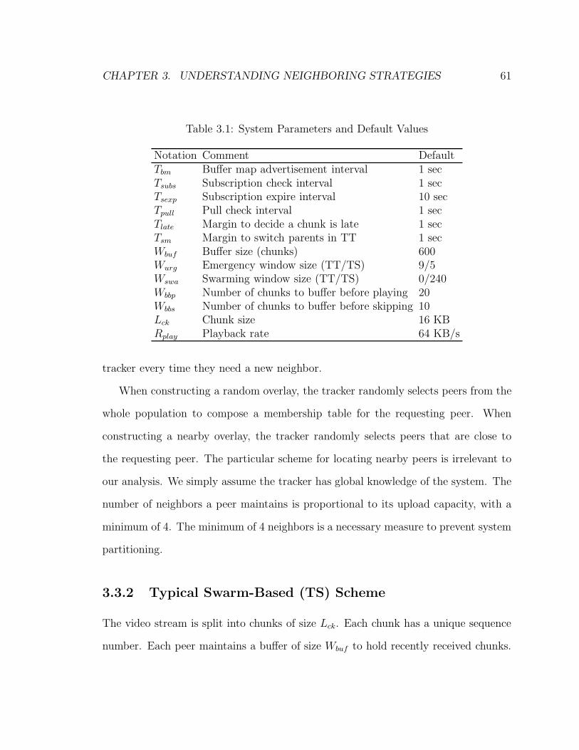
CHAPTER 3. UNDERSTANDING NEIGHBORING STRATEGIES 61
Table 3.1: System Parameters and Default Values
Notation Comment DefaultTbm Buffer map advertisement interval 1 secTsubs Subscription check interval 1 secTsexp Subscription expire interval 10 secTpull Pull check interval 1 secTlate Margin to decide a chunk is late 1 secTsm Margin to switch parents in TT 1 secWbuf Buffer size (chunks) 600Wurg Emergency window size (TT/TS) 9/5Wswa Swarming window size (TT/TS) 0/240Wbbp Number of chunks to buffer before playing 20Wbbs Number of chunks to buffer before skipping 10Lck Chunk size 16 KBRplay Playback rate 64 KB/s
tracker every time they need a new neighbor.
When constructing a random overlay, the tracker randomly selects peers from the
whole population to compose a membership table for the requesting peer. When
constructing a nearby overlay, the tracker randomly selects peers that are close to
the requesting peer. The particular scheme for locating nearby peers is irrelevant to
our analysis. We simply assume the tracker has global knowledge of the system. The
number of neighbors a peer maintains is proportional to its upload capacity, with a
minimum of 4. The minimum of 4 neighbors is a necessary measure to prevent system
partitioning.
3.3.2 Typical Swarm-Based (TS) Scheme
The video stream is split into chunks of size Lck. Each chunk has a unique sequence
number. Each peer maintains a buffer of size Wbuf to hold recently received chunks.

CHAPTER 3. UNDERSTANDING NEIGHBORING STRATEGIES 62
Every interval of length Tbm, each peer advertises its buffer map to neighbors. The
message consists of the most recent chunk’s sequence number n and a vector, whose
ith element indicates whether the peer has chunk n − i. The media player reads
chunks in the buffer and plays them back. If the player is about to play a chunk but
the chunk is unavailable, the player blocks. It resumes playing the chunk when the
chunk arrives or skips to the next available chunk if the peer has Wbbs consecutive
chunks after the chunk. Notations are shown in Table 3.1.
As in other swarm-based schemes, the buffer is sequentially divided into an emer-
gency window, which consists of chunks approaching playback deadlines, and a swarm-
ing window. Every interval of length Tpull, a peer selects all the chunks in the emer-
gency window and the rarest chunks in the swarming window to pull from neighbors.
The pull target selection algorithm is similar to that in [52, 86], which has a high
pull success rate. Assume a peer wants to pull m chunks from n neighbors, and each
neighbor has certain chunks. The algorithm starts with chunks that are available
from only 1 peer, then chunks available from 2 peers, and so on. In each step, urgent
chunks are considered before rare chunks, and a random neighbor is selected if more
than one qualified neighbor exists. A new peer first swarms until 34
of its swarming
window is filled, then it starts playing after receiving Wbbp consecutive chunks. A peer
has at most n outstanding pull requests. This measure serves as a coarse bandwidth
control for peer’s incoming pull traffic.
3.3.3 Typical Tree-Based (TT) Scheme
TT makes the following modifications to TS. Every interval of length Tsubs, a peer
checks whether to switch parents. Neighbors are ranked according to their positions

CHAPTER 3. UNDERSTANDING NEIGHBORING STRATEGIES 63
in the stream. The neighbor with the most recent position is the candidate parent.
A peer’ child cannot be its candidate parent. A peer switches parents only when the
candidate parent has a margin of Tsm more than the current parent. A child must
subscribe to its parent periodically to keep its status as a child. Peers employ the
CAC and preemption mechanisms when handling subscription requests. When peer
x receives a request from peer y, peer x grants the request if it has spare upload
capacity. Otherwise, peer x compares the upload capacity of peer y with the child z
that has the minimum upload capacity, and replaces child z with peer y if child z’s
capacity is smaller.
A peer pushes a chunk to its children immediately after receiving it and guarantees
the capacity allocated to its children. Peers only pull urgent chunks and chunks
that are Tlate seconds later than their due time. A peer uses the same pull target
selection algorithm as in TS. Note that a peer grants pull requests only if it has spare
upload capacity after serving children. A new peer starts playing after having Wbbp
consecutive chunks.
3.4 Simulation Study
In this section we study system performance of TS and TT on the random and nearby
overlay by simulation. We use the performance metrics defined in Section 2.7 As we
will show later, system performance is highly related to the shape of propagation
trees, which are described by the tree height and the average root path length of
peers, both in terms of overlay hops. (In this thesis, we say an overlay path is long
or short depending on its hop count.) We only count propagation trees that have
reached more than 90% of all of the peers when taking averages.
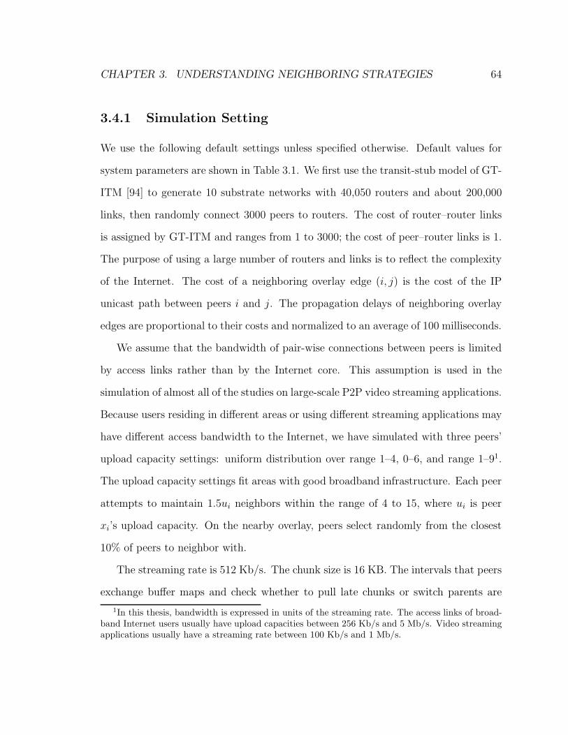
CHAPTER 3. UNDERSTANDING NEIGHBORING STRATEGIES 64
3.4.1 Simulation Setting
We use the following default settings unless specified otherwise. Default values for
system parameters are shown in Table 3.1. We first use the transit-stub model of GT-
ITM [94] to generate 10 substrate networks with 40,050 routers and about 200,000
links, then randomly connect 3000 peers to routers. The cost of router–router links
is assigned by GT-ITM and ranges from 1 to 3000; the cost of peer–router links is 1.
The purpose of using a large number of routers and links is to reflect the complexity
of the Internet. The cost of a neighboring overlay edge (i, j) is the cost of the IP
unicast path between peers i and j. The propagation delays of neighboring overlay
edges are proportional to their costs and normalized to an average of 100 milliseconds.
We assume that the bandwidth of pair-wise connections between peers is limited
by access links rather than by the Internet core. This assumption is used in the
simulation of almost all of the studies on large-scale P2P video streaming applications.
Because users residing in different areas or using different streaming applications may
have different access bandwidth to the Internet, we have simulated with three peers’
upload capacity settings: uniform distribution over range 1–4, 0–6, and range 1–91.
The upload capacity settings fit areas with good broadband infrastructure. Each peer
attempts to maintain 1.5ui neighbors within the range of 4 to 15, where ui is peer
xi’s upload capacity. On the nearby overlay, peers select randomly from the closest
10% of peers to neighbor with.
The streaming rate is 512 Kb/s. The chunk size is 16 KB. The intervals that peers
exchange buffer maps and check whether to pull late chunks or switch parents are
1In this thesis, bandwidth is expressed in units of the streaming rate. The access links of broad-band Internet users usually have upload capacities between 256 Kb/s and 5 Mb/s. Video streamingapplications usually have a streaming rate between 100 Kb/s and 1 Mb/s.

CHAPTER 3. UNDERSTANDING NEIGHBORING STRATEGIES 65
all set to one second. To emulate a practical setting where peers are asynchronous,
we start peers’ interval timers with a random offset. In TS, peers have a swarming
window of 240 chunks and an emergency window of 5 chunks. In TT, peers have no
swarming window but need a larger emergency window to recover missing chunks.
All peers join the system at time 0 to emulate a “flash crowd”, the source peer
starts streaming at time 5, and the simulation ends at time 600. According to an
empirical study in [33], we set peer churn rate to 10% of the population per minute.
From time 10, one peer is turned off every 0.2 seconds until 600 peers are turned off
at time 130. Then every 0.2 seconds, one peer is turned off and one previously turned
off peer is turned on. Statistics are collected on the 1500 peers that have never been
turned off. At time 5, we dump the neighboring overlay to compute the shortest path
tree. Each test is run 10 times using the 10 substrate networks and the average is
reported.
3.4.2 Simulation Results
We report the results of using the U(0, 6) upload setting as the base case, and report
the results of using the other two upload settings only when they lead to different
conclusions.
Tree Cost
Fig. 3.1 shows the average edge cost of overlays and propagation trees. As expected,
the neighbor-with-nearby-peers strategy greatly reduces the tree cost. TT has a
slightly lower tree cost than TS on both overlays. This phenomenon is consistent on
all of the ten topologies, indicating that TT has some capability to select low-cost

CHAPTER 3. UNDERSTANDING NEIGHBORING STRATEGIES 66
0.4
0.6
0.8
1
0 1 2 3 4 5 6 7 8 9
Ave
rag
e E
dg
e C
ost
of
Ove
rla
ys a
nd
Tre
es
Topology Index
Random Ov.TT on Random Ov.TS on Random Ov.
Nearby Ov.TT on Nearby Ov.TS on Nearby Ov.
Figure 3.1: Average overlay and propagation tree edge cost in TT and TS, normalizedwith the average cost of all the pair-wise edges between peers in the system.
paths. Also note that on the nearby overlay, the average cost of propagation tree
edges is slightly higher than overlay edges for both schemes, indicating that high-cost
edges are more heavily used on the nearby overlay.
Playback Delay and Tree Shape
Table 3.2 summarizes the playback delay and propagation tree height. The chunk
delivery delay is similar on the two overlays. The chunk buffering delay is mainly a
design choice and hence the playback delay is similar on the two overlays. In TS, a
large chunk buffering delay has to be used because the chunk delivery delay has a
large variance. In TT, the main purpose of the chunk buffering delay is to allow peers
to pull chunks that are not pushed, and a delay of of several seconds suffices. In our
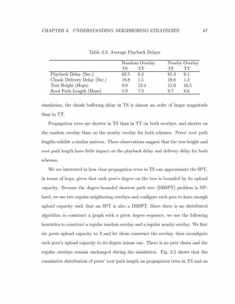
CHAPTER 3. UNDERSTANDING NEIGHBORING STRATEGIES 67
Table 3.2: Average Playback Delays
Random Overlay Nearby OverlayTS TT TS TT
Playback Delay (Sec.) 62.5 6.2 65.3 6.1Chunk Delivery Delay (Sec.) 18.8 1.5 18.8 1.3Tree Height (Hops) 9.0 13.4 11.0 16.5Root Path Length (Hops) 5.9 7.3 6.7 8.6
simulation, the chunk buffering delay in TS is almost an order of larger magnitude
than in TT.
Propagation trees are shorter in TS than in TT on both overlays, and shorter on
the random overlay than on the nearby overlay for both schemes. Peers’ root path
lengths exhibit a similar pattern. These observations suggest that the tree height and
root path length have little impact on the playback delay and delivery delay for both
schemes.
We are interested in how close propagation trees in TS can approximate the SPT,
in terms of hops, given that each peer’s degree on the tree is bounded by its upload
capacity. Because the degree-bounded shortest path tree (DBSPT) problem is NP-
hard, we use two regular neighboring overlays and configure each peer to have enough
upload capacity such that an SPT is also a DBSPT. Since there is no distributed
algorithm to construct a graph with a given degree sequence, we use the following
heuristics to construct a regular random overlay and a regular nearby overlay. We first
set peers upload capacity to 3 and let them construct the overlay, then reconfigure
each peer’s upload capacity to its degree minus one. There is no peer churn and the
regular overlays remain unchanged during the simulation. Fig. 3.2 shows that the
cumulative distribution of peers’ root path length on propagation trees in TS and on
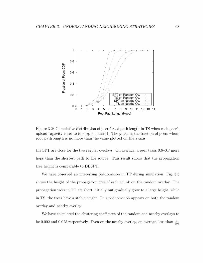
CHAPTER 3. UNDERSTANDING NEIGHBORING STRATEGIES 68
0
0.2
0.4
0.6
0.8
1
0 1 2 3 4 5 6 7 8 9 10 11 12 13 14
Fra
ctio
n o
f P
ee
rs C
DF
Root Path Length (Hops)
SPT on Random Ov.TS on Random Ov.SPT on Nearby Ov.
TS on Nearby Ov.
Figure 3.2: Cumulative distribution of peers’ root path length in TS when each peer’supload capacity is set to its degree minus 1. The y-axis is the fraction of peers whoseroot path length is no more than the value plotted on the x-axis.
the SPT are close for the two regular overlays. On average, a peer takes 0.6–0.7 more
hops than the shortest path to the source. This result shows that the propagation
tree height is comparable to DBSPT.
We have observed an interesting phenomenon in TT during simulation. Fig. 3.3
shows the height of the propagation tree of each chunk on the random overlay. The
propagation trees in TT are short initially but gradually grow to a large height, while
in TS, the trees have a stable height. This phenomenon appears on both the random
overlay and nearby overlay.
We have calculated the clustering coefficient of the random and nearby overlays to
be 0.002 and 0.025 respectively. Even on the nearby overlay, on average, less than 1200
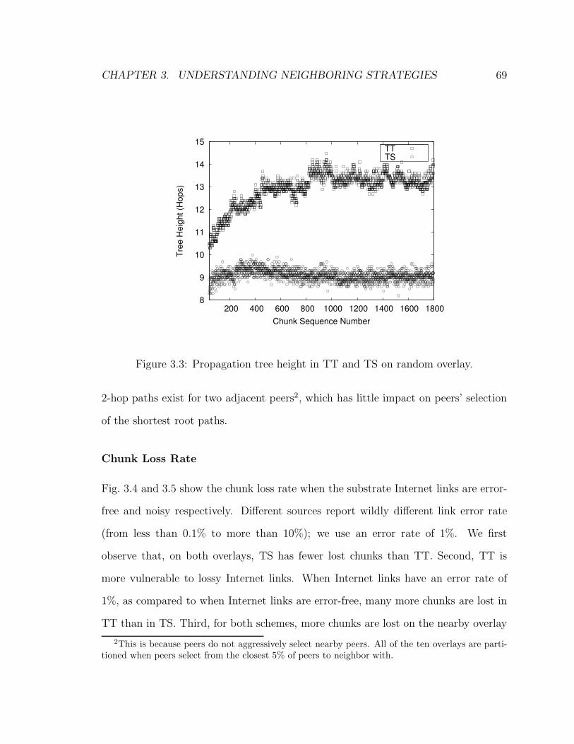
CHAPTER 3. UNDERSTANDING NEIGHBORING STRATEGIES 69
8
9
10
11
12
13
14
15
200 400 600 800 1000 1200 1400 1600 1800
Tre
e H
eig
ht
(Ho
ps)
Chunk Sequence Number
TT TS
Figure 3.3: Propagation tree height in TT and TS on random overlay.
2-hop paths exist for two adjacent peers2, which has little impact on peers’ selection
of the shortest root paths.
Chunk Loss Rate
Fig. 3.4 and 3.5 show the chunk loss rate when the substrate Internet links are error-
free and noisy respectively. Different sources report wildly different link error rate
(from less than 0.1% to more than 10%); we use an error rate of 1%. We first
observe that, on both overlays, TS has fewer lost chunks than TT. Second, TT is
more vulnerable to lossy Internet links. When Internet links have an error rate of
1%, as compared to when Internet links are error-free, many more chunks are lost in
TT than in TS. Third, for both schemes, more chunks are lost on the nearby overlay
2This is because peers do not aggressively select nearby peers. All of the ten overlays are parti-tioned when peers select from the closest 5% of peers to neighbor with.
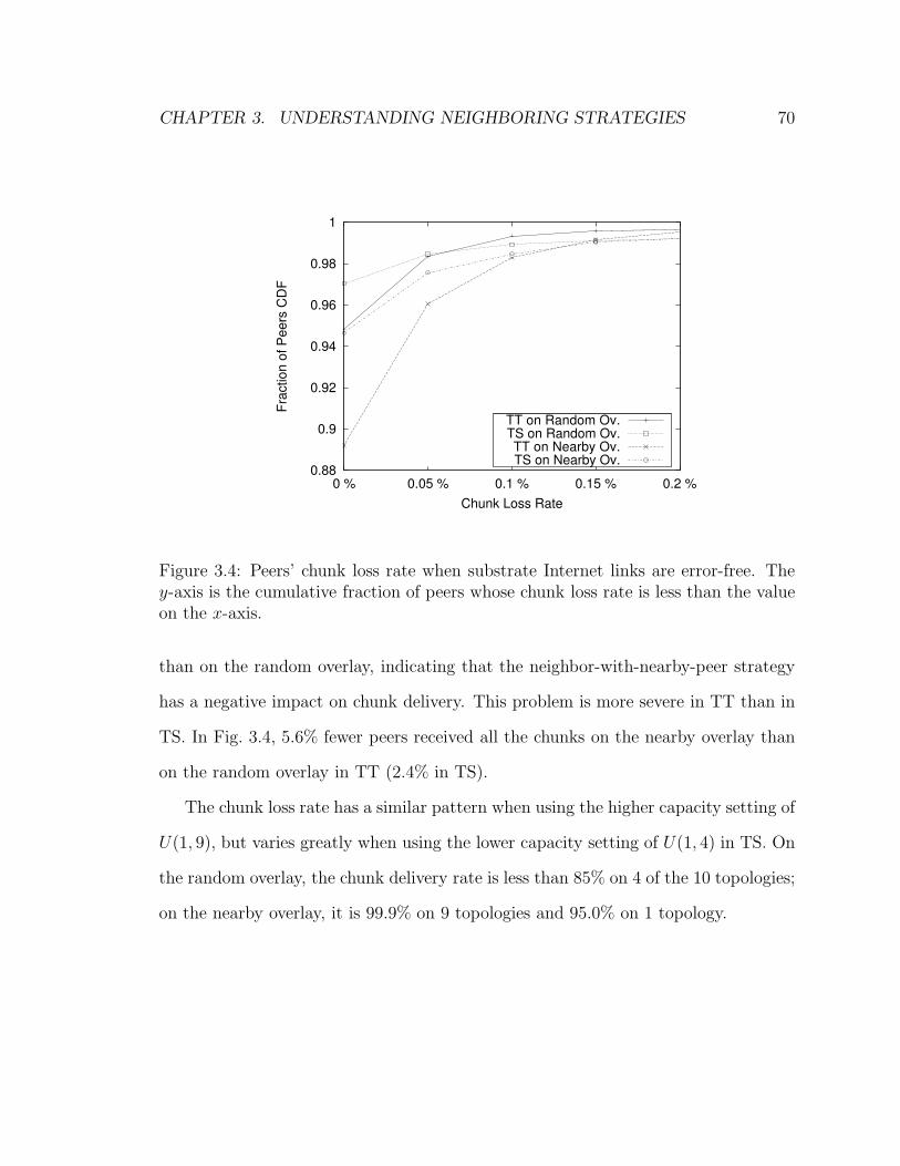
CHAPTER 3. UNDERSTANDING NEIGHBORING STRATEGIES 70
0.88
0.9
0.92
0.94
0.96
0.98
1
0 % 0.05 % 0.1 % 0.15 % 0.2 %
Fra
ctio
n o
f P
ee
rs C
DF
Chunk Loss Rate
TT on Random Ov.TS on Random Ov.TT on Nearby Ov.TS on Nearby Ov.
Figure 3.4: Peers’ chunk loss rate when substrate Internet links are error-free. They-axis is the cumulative fraction of peers whose chunk loss rate is less than the valueon the x-axis.
than on the random overlay, indicating that the neighbor-with-nearby-peer strategy
has a negative impact on chunk delivery. This problem is more severe in TT than in
TS. In Fig. 3.4, 5.6% fewer peers received all the chunks on the nearby overlay than
on the random overlay in TT (2.4% in TS).
The chunk loss rate has a similar pattern when using the higher capacity setting of
U(1, 9), but varies greatly when using the lower capacity setting of U(1, 4) in TS. On
the random overlay, the chunk delivery rate is less than 85% on 4 of the 10 topologies;
on the nearby overlay, it is 99.9% on 9 topologies and 95.0% on 1 topology.
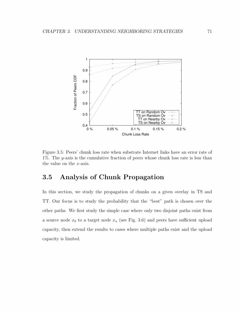
CHAPTER 3. UNDERSTANDING NEIGHBORING STRATEGIES 71
0.4
0.5
0.6
0.7
0.8
0.9
1
0 % 0.05 % 0.1 % 0.15 % 0.2 %
Fra
ctio
n o
f P
ee
rs C
DF
Chunk Loss Rate
TT on Random OvTS on Random OvTT on Nearby OvTS on Nearby Ov
Figure 3.5: Peers’ chunk loss rate when substrate Internet links have an error rate of1%. The y-axis is the cumulative fraction of peers whose chunk loss rate is less thanthe value on the x-axis.
3.5 Analysis of Chunk Propagation
In this section, we study the propagation of chunks on a given overlay in TS and
TT. Our focus is to study the probability that the “best” path is chosen over the
other paths. We first study the simple case where only two disjoint paths exist from
a source node x0 to a target node xn (see Fig. 3.6) and peers have sufficient upload
capacity, then extend the results to cases where multiple paths exist and the upload
capacity is limited.

CHAPTER 3. UNDERSTANDING NEIGHBORING STRATEGIES 72
x0
y0
xn
ym
x1
ym-1
xn-1
y1
x2
Figure 3.6: Two disjoint paths with n and m hops, n > m. The leftmost peer isdenoted as x0 and y0 and the rightmost peer as xn and ym for convenience.
Table 3.3: Notations Used in Propagation and Overlay Model
Notation Commentg The gap from the checking time to the advertising timeδ A U(0, 1) random variablefi, Fi The PDF and CDF of the sum of i U(0, 1)
dXij , (dYij)
The propagation delay from node xi to node xj (fromnode yi to node yj)
N The population of the P2P systemM The size of the set of nearby peersSi The set of peers close to node xiwi The weight of peer xiri The radius of set Si
3.5.1 Chunk Propagation in Typical Swarm-Based (TS) Scheme
We model the propagation of a new chunk c as follows. The impact of chunk schedul-
ing algorithm is discussed later. Assume peers’ upload capacity and overlay edges’
bandwidth are infinite, i.e., there is no transmission and queuing delay3. Let dXij
denote the propagation delay between peers xi and xj (along path xi, xi+1, . . . , xj).
3Queuing delay is the amount of time a packet waits at the sender to be transmitted; transmissiondelay is the amount of time required to push a packet onto a link; and propagation delay is the amountof time required for the head of a packet to travel from the sender to the receiver over a link.

CHAPTER 3. UNDERSTANDING NEIGHBORING STRATEGIES 73
Each peer advertises its buffer map and checks whether to pull chunks every inter-
val of length T ; the gap g from the check time to the advertise time is constant.
Peers work in an asynchronous manner, i.e., the advertise and check time of peers is
uniformly distributed on [0, T ]. Notations are described in Table 3.3.
A peer pulls a missing chunk immediately after it finds a neighbor that has the
chunk. Since there are no transmission or queuing delays, if peer xi finds a missing
chunk available at peer xi−1 at time 0, it will obtain the chunk at time 2dX(i−1)i. To
simplify the expression, we assume the interval T to be 1 time unit, i.e., time and
delays are expressed in units of T .
Preposition 1. In the typical swarm-based (TS) scheme, given two disjoint paths
(x0, x1, . . . , xn) and (x0, y1, ym−1, xn) from a source peer x0 to a target peer xn, the
probability that peer xn pulls chunks from xn−1 rather than from peer ym−1 is
Pn,m = Fm+n(m−DXn +DY
m) (3.1)
where F is the CDF of the sum of m + n i.i.d U(0, 1), DXn = ng + dX0n, and DY
m =
mg + dY0m.
Proof. Let δXi be the random variable denoting the time when peer xi−1 obtains a
chunk c to the time peer xi obtains the same chunk c. Assume peer xi−1 obtains
chunk c at time t. After fetching chunk c, it advertises its buffer map at time t + g.
The message reaches peers xi at time t+ g + dX(i−1)i. The time peer xi fetches chunk
c is uniformly distributed on (t + g + dX(i−1)i, t + g + dX(i−1)i + 1). Therefore δXi =
δXi −(g+dX(i−1)i) is a U(0, 1) random variable. Let Xi be the random variable denoting
the time from peer x0 obtains a chunk c to the time peer xi obtains chunk c. Then
Xn−DXn is the sum of n i.i.d U(0, 1). Likewise, Ym−DY
m is the sum of m i.i.d U(0, 1).
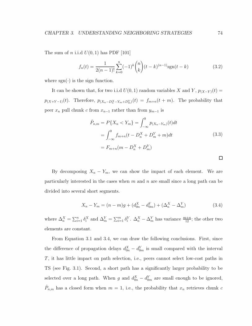
CHAPTER 3. UNDERSTANDING NEIGHBORING STRATEGIES 74
The sum of n i.i.d U(0, 1) has PDF [101]
fn(t) =1
2(n− 1)!
n∑
k=0
(−1)k(
n
k
)
(t− k)(n−1)sgn(t− k) (3.2)
where sgn(·) is the sign function.
It can be shown that, for two i.i.d U(0, 1) random variables X and Y , p(X−Y )(t) =
p(X+Y−1)(t). Therefore, p(Xn−DXn −Ym+DY
m)(t) = fm+n(t + m). The probability that
peer xn pull chunk c from xn−1 rather than from ym−1 is
Pn,m = P{Xn < Ym} =∫ 0
−∞
p(Xn−Ym)(t)dt
=∫ 0
−∞
fm+n(t−DXn +DY
m +m)dt
= Fm+n(m−DXn +DY
m)
(3.3)
By decomposing Xn − Ym, we can show the impact of each element. We are
particularly interested in the cases when m and n are small since a long path can be
divided into several short segments.
Xn − Ym = (n−m)g + (dX0n − dY0m) + (∆Xn −∆Y
m) (3.4)
where ∆Xn =
∑ni=1 δ
Xi and ∆Y
m =∑mi=1 δ
Yi . ∆X
n −∆Ym has variance m+n
12; the other two
elements are constant.
From Equation 3.1 and 3.4, we can draw the following conclusions. First, since
the difference of propagation delays dX0n − dY0m is small compared with the interval
T , it has little impact on path selection, i.e., peers cannot select low-cost paths in
TS (see Fig. 3.1). Second, a short path has a significantly larger probability to be
selected over a long path. When g and dX0n − dY0m are small enough to be ignored,
Pn,m has a closed form when m = 1, i.e., the probability that xn retrieves chunk c

CHAPTER 3. UNDERSTANDING NEIGHBORING STRATEGIES 75
from an n-hop path (x0, x1, . . . , xn) rather than a 1-hop path (y0, ym) is Pn,1 = 1(n+1)!
.
When m > 1, the probability can be calculated but has no closed form. For example,
P3,2 = 940
. Therefore TS has short propagation trees (see Table 3.2 and Fig. 3.2).
Third, a large gap g can dramatically increase the probability of short paths being
selected. For example, when g is set to its maximum value of 1 (i.e., the interval T ),
a 1-hop path will always be chosen over an n-hop (n ≥ 2) path, and a 2-hop path is
chosen over a 3-hop path with a probability of 2324
(compared with 3140
when g is 0). In
our simulation, g is set to 1. Although a large d increases the chunk delivery delay,
since pull schemes already have a playback delay of tens of seconds, setting d to its
maximum value seems to be a good trade-off.
3.5.2 Chunk Propagation in Typical Tree-Based (TT) Scheme
We model the tree-building and propagation of new chunks as follows. We also
assume that peers’ upload capacity and overlay edges’ bandwidth are infinite. Each
peer advertises its position in the stream and checks whether to switch parents every
interval of length T ; the gap g from the check time to the advertise time is constant.
We use the fluid traffic model, i.e., the reported position has a continuous space. If
peer xn finds neighbor xn−1 proceeding further in the stream than its parent ym−1, it
immediately switches to that neighbor, i.e., it becomes the child of peer xn−1 after a
time of length 2dX(n−1)n. A peer, after receiving a chunk, immediately pushes it to its
children. For example, if peer xi−1 obtains a chunk at time 0, its child xi obtains the
chunk at time dX(i−1)i. Peer x0 begins streaming as time 0.
Preposition 2. In the typical tree-based (TT) scheme, given two disjoint paths
(x0, x1, . . . , xn) and (x0, y1, ym−1, xn) from a source peer x0 to a target peer xn, (x0, . . . , xn−1)

CHAPTER 3. UNDERSTANDING NEIGHBORING STRATEGIES 76
and (x0, . . . , ym−1) are two tree branches rooted at x0, the probability that peer xn sub-
scribes to xn−1 rather than to ym−1 is
P =
0, τ ≥ 1,
12
+ τ − τ2
2, −1 ≤ τ < 1,
1, τ < −1
(3.5)
where τ = dX0n − dY0m.
Proof. Assume dX0n ≥ dY0m; the proof when dX0n < dY0m is the same. To simplify the
expressions, we assume that peer x0’s most recent position in the stream at time 0 is
0. Peer xn−1 advertises, at time tX1 , its playback position tX1 − dX0(n−1). The message
arrives at peer xn at time tX2 = tX1 + dX(n−1)n. Obviously, tX1 − dX0(n−1) = tX2 − dX0n.
Similarly, peer ym−1 advertises at time tY1 , and the message arrives at peer xn at time
tY2 = tY1 + dY(m−1)m carrying peer ym−1’s playback position tY2 − dY0m.
Since peers are asynchronous, t = tX2 − tY2 follows the U(0, 1) distribution. Let
tc denote the time peer xn attempts to switch parents. If tc ≥ tX2 , tc ≥ tY2 , and
tX1 ≥ tY1 , then peer xn will subscribe to peer xn−1; otherwise peer xn will subscribe
to peer ym−1. When dX0n ≥ dY0m + 1, the expression tX1 ≥ tY1 does not hold, hence peer
xn will always subscribe to peer ym−1. When dX0n < dY0m + 1, conditioning on t, the
probability that peer xn subscribes to peer xn−1 is
P =∫ 1
τ(1− t)dt =
1
2− τ +
τ 2
2(3.6)
Equation 3.5 shows that peers in TT choose low-cost paths with a slightly higher
probability (see Fig. 3.1), and the probability increases when using a smaller interval
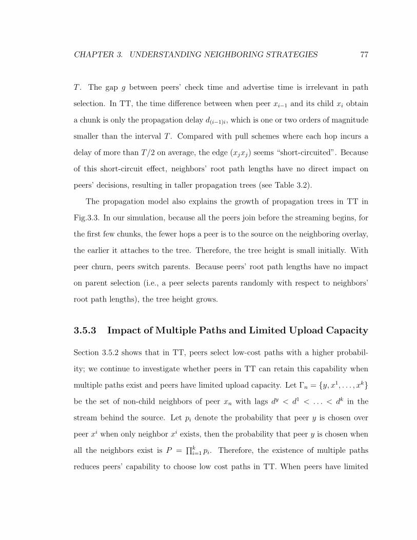
CHAPTER 3. UNDERSTANDING NEIGHBORING STRATEGIES 77
T . The gap g between peers’ check time and advertise time is irrelevant in path
selection. In TT, the time difference between when peer xi−1 and its child xi obtain
a chunk is only the propagation delay d(i−1)i, which is one or two orders of magnitude
smaller than the interval T . Compared with pull schemes where each hop incurs a
delay of more than T/2 on average, the edge (xjxj) seems “short-circuited”. Because
of this short-circuit effect, neighbors’ root path lengths have no direct impact on
peers’ decisions, resulting in taller propagation trees (see Table 3.2).
The propagation model also explains the growth of propagation trees in TT in
Fig.3.3. In our simulation, because all the peers join before the streaming begins, for
the first few chunks, the fewer hops a peer is to the source on the neighboring overlay,
the earlier it attaches to the tree. Therefore, the tree height is small initially. With
peer churn, peers switch parents. Because peers’ root path lengths have no impact
on parent selection (i.e., a peer selects parents randomly with respect to neighbors’
root path lengths), the tree height grows.
3.5.3 Impact of Multiple Paths and Limited Upload Capacity
Section 3.5.2 shows that in TT, peers select low-cost paths with a higher probabil-
ity; we continue to investigate whether peers in TT can retain this capability when
multiple paths exist and peers have limited upload capacity. Let Γn = {y, x1, . . . , xk}
be the set of non-child neighbors of peer xn with lags dy < d1 < . . . < dk in the
stream behind the source. Let pi denote the probability that peer y is chosen over
peer xi when only neighbor xi exists, then the probability that peer y is chosen when
all the neighbors exist is P =∏ki=1 pi. Therefore, the existence of multiple paths
reduces peers’ capability to choose low cost paths in TT. When peers have limited

CHAPTER 3. UNDERSTANDING NEIGHBORING STRATEGIES 78
upload capacity, the value of τ in Equation 3.5 is augmented to include the queu-
ing and transmission delays. When overlay edges have stable bandwidth and peers
employ CAC, the transmission delay is constant given the overlay edge bandwidth.
When peers employ CAC, queuing delays at each peer have a small variance, and the
queuing and transmission delays are proportional to path length. Therefore, peers’
capability to select low-cost paths decreases when peers have limited upload capacity,
but the capability to select short paths increases. In practical settings, these changes
are small because the interval T is typically one or two orders of magnitude larger
than the propagation, queueing, and transmission delays.
Peers may rank neighbors to decide which subscription request to grant when
receiving multiple requests but having insufficient bandwidth. They may also use a
preemption mechanism to deal with the situation when requests from preferred peers
arrive later. In this case, the set Γn contains only high-ranking neighbors, which
further reduces peers’ capability to select low cost paths.
Section 3.5.1 shows that TS can select short paths; we continue to investigate
whether it can retain this capability when multiple paths exist and peers have limited
upload capacity. Assume ~y, ~x1, . . . , ~xk are disjoint paths from x0 to xn, and let pi
denote the probability that path ~y is chosen over path ~xi when only the two paths
exist, then the probability that path ~y is chosen when all the paths exist is P =∏ki=1 pi.
When alternate paths are not disjoint, the probability cannot be expressed in a closed
form. As a rule of thumb, adding cross edges between alternate paths ~x1, . . . , ~xk
decreases the probability that path ~y is chosen. Equation 3.1 indicates that a long
path has a significant lower probability to be chosen, and hence whether TS can
select short paths depends on the number of short alternate paths (we will discuss
CHAPTER 3. UNDERSTANDING NEIGHBORING STRATEGIES 79
the number of alternative paths in Section 3.6). When peers have limited upload
capacities, although the value of Xn − Ym in Equation 3.4 is augmented to include
queuing and transmission delays at each hop, they are too small to have any impact.
3.6 Analysis of the Impact of Overlays
In this section, we analyze the impact of the neighbor-with-nearby-peers strategy on
system performance. We first introduce the random graph model that is used to
construct the random and nearby overlays, then compare their properties that have
the most impact on system performance, and finally, together with packet propagation
models, analyze these properties’ impact on system performance in the two typical
schemes.
3.6.1 Properties of Random and Nearby Overlays
A number of random graph models exist that produce different distributions of nodes
and edges on the graph. Like most Internet topology generators, we use the Erdos–
Renyi model G(N, p) to construct the random and nearby overlays. First N nodes
are randomly placed on a plane, and then for each pair of nodes, an edge is added
with probability p. The Euclidean distance on the plane between two nodes is their
overlay edge’s cost. We use the terms distance and cost interchangeably. Let w
denote the desired average node degree on the neighboring overlay. On the random
overlay, the probability p is set to µ = wN
. The random graph is expected to have wN
edges (including w self loops). On the nearby overlay, we only add edges between
nearby nodes. Let Si be the set of M nodes that are closest to node xi. Let ri be the
CHAPTER 3. UNDERSTANDING NEIGHBORING STRATEGIES 80
distance between node xi and the farthest node in Si. For a pair of nodes xi and xj ,
the probability p is set to ν = wM
if xi ∈ Sj and xj ∈ Si and to 0 otherwise. Since
M is several orders of magnitude smaller than N , ν ≫ µ. We remark that if peers
greedily neighbor with nearby peers, the resulting overlay is inevitably partitioned; a
certain amount of randomness must be employed. Notations are shown in Table 3.3.
On the random overlay, each node xi has a weight wi. An edge exists between an
arbitrary pair of nodes xi and xj with a probability of ξwiwj, where ξ is a normalizing
coefficient. Let w be the expected degree of nodes, then
ξ =Nw
(
∑Ni=1wi
)2
The random graph is expected to have wN edges4. If all the nodes have the same
weight w, two arbitrary nodes are adjacent with a probability of µ = wN
, and each
node is expected to have w neighbors. If all the nodes have the same weight w, two
nearby nodes are adjacent with a probability of ν = wM
. If ri > rj, node i may be
adjacent with a node k not in Si but in Sj . Each node has its own expected degree.
The expected number of edges of the graph is unknown as well.
The overlay properties that have the most impact on system performance include
edge cost, diameter, connectivity, and clustering coefficient. Obviously, the nearby
overlay has a lower edge cost and a larger diameter than the random overlay. The
Meridian project [93] measured the delays between 2500 hosts on the Internet. The
average of all the delays was 77 milliseconds. By contrast, the average of the shortest
10% delays is 12 milliseconds and the shortest 5% delays is 7.8 milliseconds. If peers
only neighbor with the closest 10% of peers, the resulting nearby overlay will have
4This number includes ξ∑
N
i=1w2
iself loops.
CHAPTER 3. UNDERSTANDING NEIGHBORING STRATEGIES 81
much shorter edges than a random overlay5. The random graph has a diameter of
O(logN). The nearby overlay has a diameter of O(N1
α ), where α is the dimension
of the space in which nodes are placed (α equals 2 in our case). The connectivity
of a graph measures how easily a graph can be partitioned. The nearby overlay is
more prone to partitioning than the random overlay, especially in the presence of peer
churn. Temporary partitioning is tolerable in file sharing applications, but greatly
degrades the quality of video streaming service. We find that the system may be
partitioned even when peers neighbor with the closest 10% of peers. The clustering
coefficient measures the extent to which peers cluster together. It is defined as the
number of closed triplets over the total number of triplets on a graph. (A triplet
is three nodes that are connected by either two edges or three edges; in the latter
case, it is called a closed triplet.) The nearby overlay has a much larger clustering
coefficient than the random overlay.
When a neighboring overlay has a high clustering coefficient, for each edge, there
tend to be more short alternate paths. As discussed in the propagation model, this
will have an impact on the probability that a peer chooses the “best” path. We
quantitatively analyze the number of short alternate paths on the random and nearby
overlays in the following two prepositions.
Preposition 3. On a random overlay, the expected number of l-hop paths between
two arbitrary nodes is O( 1N
) when l is small and N is large.
Proof. Let P be the matrix where the (i, j)-th element pi,j denotes the probability
that an edge exists between nodes i and j. Let Q be the matrix where qi,j denotes
the probability that a path of length n exists between node i and j. Let Q′ be the
5The actual cost saving of the neighbor-with-nearby-peers strategy is significant but less thanthese numbers suggested because peers are not evenly placed on the plane.
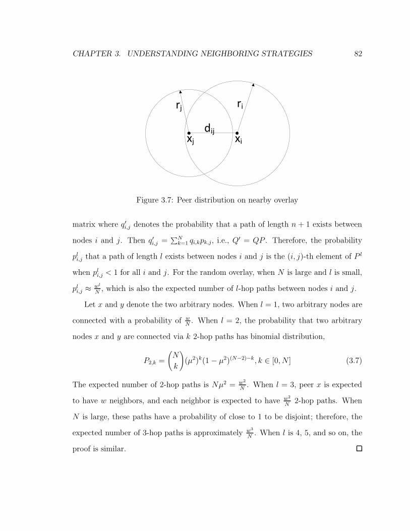
CHAPTER 3. UNDERSTANDING NEIGHBORING STRATEGIES 82
xi
rirj
xjdij
Figure 3.7: Peer distribution on nearby overlay
matrix where q′i,j denotes the probability that a path of length n + 1 exists between
nodes i and j. Then q′i,j =∑Nk=1 qi,kpk,j, i.e., Q′ = QP . Therefore, the probability
pli,j that a path of length l exists between nodes i and j is the (i, j)-th element of P l
when pli,j < 1 for all i and j. For the random overlay, when N is large and l is small,
pli,j ≈ wl
N, which is also the expected number of l-hop paths between nodes i and j.
Let x and y denote the two arbitrary nodes. When l = 1, two arbitrary nodes are
connected with a probability of wN
. When l = 2, the probability that two arbitrary
nodes x and y are connected via k 2-hop paths has binomial distribution,
P2,k =
(
N
k
)
(µ2)k(1− µ2)(N−2)−k, k ∈ [0, N ] (3.7)
The expected number of 2-hop paths is Nµ2 = w2
N. When l = 3, peer x is expected
to have w neighbors, and each neighbor is expected to have w2
N2-hop paths. When
N is large, these paths have a probability of close to 1 to be disjoint; therefore, the
expected number of 3-hop paths is approximately w3
N. When l is 4, 5, and so on, the
proof is similar.

CHAPTER 3. UNDERSTANDING NEIGHBORING STRATEGIES 83
Preposition 4. On a random overlay, the expected number of l-hop paths between
an arbitrary pair of adjacent nodes is O(1) when l is small.
Proof. Assume nodes xi and xj have wi and wj neighbors respectively. We first find
the expected number of nodes that are in both Si and Sj. Without loss of generality,
we assume ri ≥ rj . Let cij denote the distance (substrate IP path cost) between
node xi and xj . For an arbitrary node in Sj, the probability ψ that it is in Si is the
proportion of the intersection of the two circles in Fig. 3.7. When cij = 0, the two
sets Si and Sj are equal and ψ is 1. When cij = ri = rj , ψ has its minimum value,
ψ =23πr2 −
√3r2
πr2≈ 0.12 (3.8)
Assuming Si and Sj have M ′ common nodes, the probability Q2,k that nodes xi
and xj is connected via k 2-hop path is
Q2,k ≥(
M ′
k
)
(ν2)k(1− ν2)M′−k, k ∈ [0,M ′] (3.9)
where the greater sign comes from the fact that nodes xi and xj may be connected via
a node not in Si or Sj . Since the distribution of nodes on the plane and the probability
of an edge existing between two peers are independent, the expected number of 2-hop
paths is no less than M ′ν2 = ψwiwj
M, where ψ ∈ [0.12, 1].
On average, node xj has ψwj adjacent nodes in the intersection area; each node
has M ′ν2 = ψw2
M2-hop paths to node xi (assuming they have w neighbors). Although
some paths are not edge-disjoint, the number of 3-hop edges is still O(1). The proofs
for l = 2, 3, . . . are similar. Note that the total number of edge-disjoint paths are
bounded by min{wi, wj}.
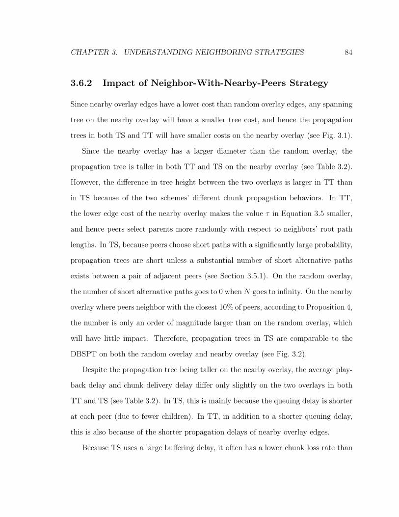
CHAPTER 3. UNDERSTANDING NEIGHBORING STRATEGIES 84
3.6.2 Impact of Neighbor-With-Nearby-Peers Strategy
Since nearby overlay edges have a lower cost than random overlay edges, any spanning
tree on the nearby overlay will have a smaller tree cost, and hence the propagation
trees in both TS and TT will have smaller costs on the nearby overlay (see Fig. 3.1).
Since the nearby overlay has a larger diameter than the random overlay, the
propagation tree is taller in both TT and TS on the nearby overlay (see Table 3.2).
However, the difference in tree height between the two overlays is larger in TT than
in TS because of the two schemes’ different chunk propagation behaviors. In TT,
the lower edge cost of the nearby overlay makes the value τ in Equation 3.5 smaller,
and hence peers select parents more randomly with respect to neighbors’ root path
lengths. In TS, because peers choose short paths with a significantly large probability,
propagation trees are short unless a substantial number of short alternative paths
exists between a pair of adjacent peers (see Section 3.5.1). On the random overlay,
the number of short alternative paths goes to 0 whenN goes to infinity. On the nearby
overlay where peers neighbor with the closest 10% of peers, according to Proposition 4,
the number is only an order of magnitude larger than on the random overlay, which
will have little impact. Therefore, propagation trees in TS are comparable to the
DBSPT on both the random overlay and nearby overlay (see Fig. 3.2).
Despite the propagation tree being taller on the nearby overlay, the average play-
back delay and chunk delivery delay differ only slightly on the two overlays in both
TT and TS (see Table 3.2). In TS, this is mainly because the queuing delay is shorter
at each peer (due to fewer children). In TT, in addition to a shorter queuing delay,
this is also because of the shorter propagation delays of nearby overlay edges.
Because TS uses a large buffering delay, it often has a lower chunk loss rate than

CHAPTER 3. UNDERSTANDING NEIGHBORING STRATEGIES 85
TT and is more robust when Internet links are erroneous (see Figs. 3.4 and 3.5).
Now we discuss the impact of the overlays on the chunk loss rate. When peers lack
upload capacity to send all the chunks to all the requesting neighbors, or peer churn
and substrate network errors exist, chunks propagate along different paths. When a
neighboring overlay has a higher clustering coefficient, the root path of a peer tends
to be more “similar”, i.e., these paths share more common nodes and edges and have
similar hop counts. Therefore, compared with the random overlay, on the nearby
overlay, chunks tend to propagate along a group of longer but similar paths. This
property has a different impact on the chunk loss rate in TT and TS because of their
different chunk propagation behaviors.
In TT, a peer attempts to pull all the chunks not pushed by its parent. The fewer
chunks that need to be pulled and the higher the pull success rate, the higher the
chunk delivery rate. Because TT has a short playback delay, if a chunk is late at a
peer, its descendants may also need to pull the chunk. On the random overlay, these
peers have different neighbors to pull the chunk from. On the nearby overlay, these
peers share many common neighbors; it is hard for them to find neighbors with the
chunk and spare upload capacity in a short time. Therefore, the pull success rate is
lower and hence more chunks are in TT on the nearby overlay (see Figs. 3.4 and 3.5).
In TS, for a chunk c, at each hop and in each interval, the peer may decide
to pull chunks other than chunk c, causing chunk c to miss its playback deadline.
Therefore, longer root paths on the nearby overlay usually cause more lost chunks in
TS, but because swarm-based schemes typically have a large chunk buffering delay,
the increase is usually not severe (see Figs. 3.4 and 3.5).
Because chunks propagate along a group of similar paths on the nearby overlay, the
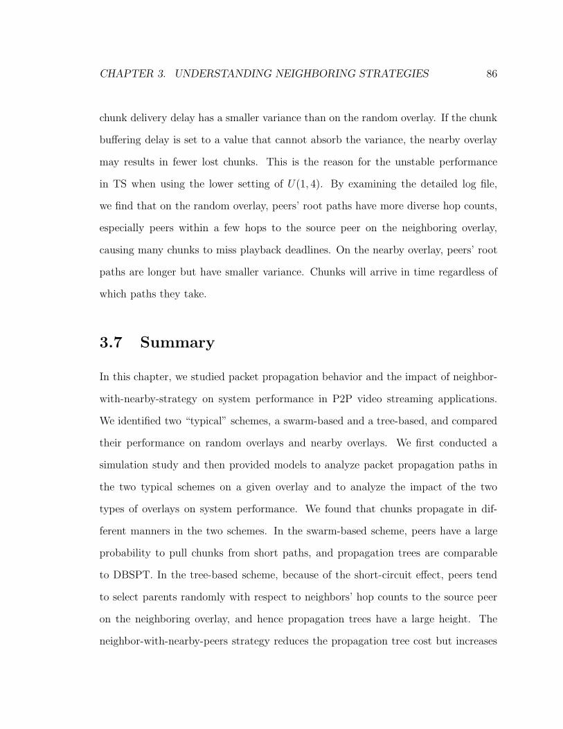
CHAPTER 3. UNDERSTANDING NEIGHBORING STRATEGIES 86
chunk delivery delay has a smaller variance than on the random overlay. If the chunk
buffering delay is set to a value that cannot absorb the variance, the nearby overlay
may results in fewer lost chunks. This is the reason for the unstable performance
in TS when using the lower setting of U(1, 4). By examining the detailed log file,
we find that on the random overlay, peers’ root paths have more diverse hop counts,
especially peers within a few hops to the source peer on the neighboring overlay,
causing many chunks to miss playback deadlines. On the nearby overlay, peers’ root
paths are longer but have smaller variance. Chunks will arrive in time regardless of
which paths they take.
3.7 Summary
In this chapter, we studied packet propagation behavior and the impact of neighbor-
with-nearby-strategy on system performance in P2P video streaming applications.
We identified two “typical” schemes, a swarm-based and a tree-based, and compared
their performance on random overlays and nearby overlays. We first conducted a
simulation study and then provided models to analyze packet propagation paths in
the two typical schemes on a given overlay and to analyze the impact of the two
types of overlays on system performance. We found that chunks propagate in dif-
ferent manners in the two schemes. In the swarm-based scheme, peers have a large
probability to pull chunks from short paths, and propagation trees are comparable
to DBSPT. In the tree-based scheme, because of the short-circuit effect, peers tend
to select parents randomly with respect to neighbors’ hop counts to the source peer
on the neighboring overlay, and hence propagation trees have a large height. The
neighbor-with-nearby-peers strategy reduces the propagation tree cost but increases

CHAPTER 3. UNDERSTANDING NEIGHBORING STRATEGIES 87
the risk of system partitioning and causes more lost chunks. The different chunk
propagation behaviors of the swarm-based and tree-based schemes cause chunk loss
in different ways in the two schemes. The neighbor-with-nearby-peers strategy causes
more chunk loss in the tree-based schemes than in the swarm-based schemes.

Chapter 4
ISP-Friendly P2P Live Streaming
4.1 Introduction
In Chapter 3, we have shown that using the neighbor-with-nearby-peers strategy can
reduce network traffic but also result in a neighboring overlay which is prone to par-
titioning, a multicast tree with a large height, and more lost chunks in the presence
of peer churn and Internet link errors. In this chapter, we propose a neighboring
strategy to construct a hierarchical overlay and a network-driven tree-building algo-
rithm. Our idea is to first identify the desired shape of propagation trees, then to
construct the neighboring overlay to be the super graph of these trees, and to use
the tree-building algorithm to construct trees with the desired shape on the neigh-
boring overlay. On the hierarchical overlay, most edges are between nearby peers to
reduce network traffic, but a small fraction of edges are rewired to remote peers in a
way that the neighboring overlay exhibits a hierarchical structure. The tree-building
algorithm, called TreeClimber, is a distance-vector (DV)-style routing protocol; it
heuristically constructs a DBMST, with respect to hops, on a neighboring overlay.
88
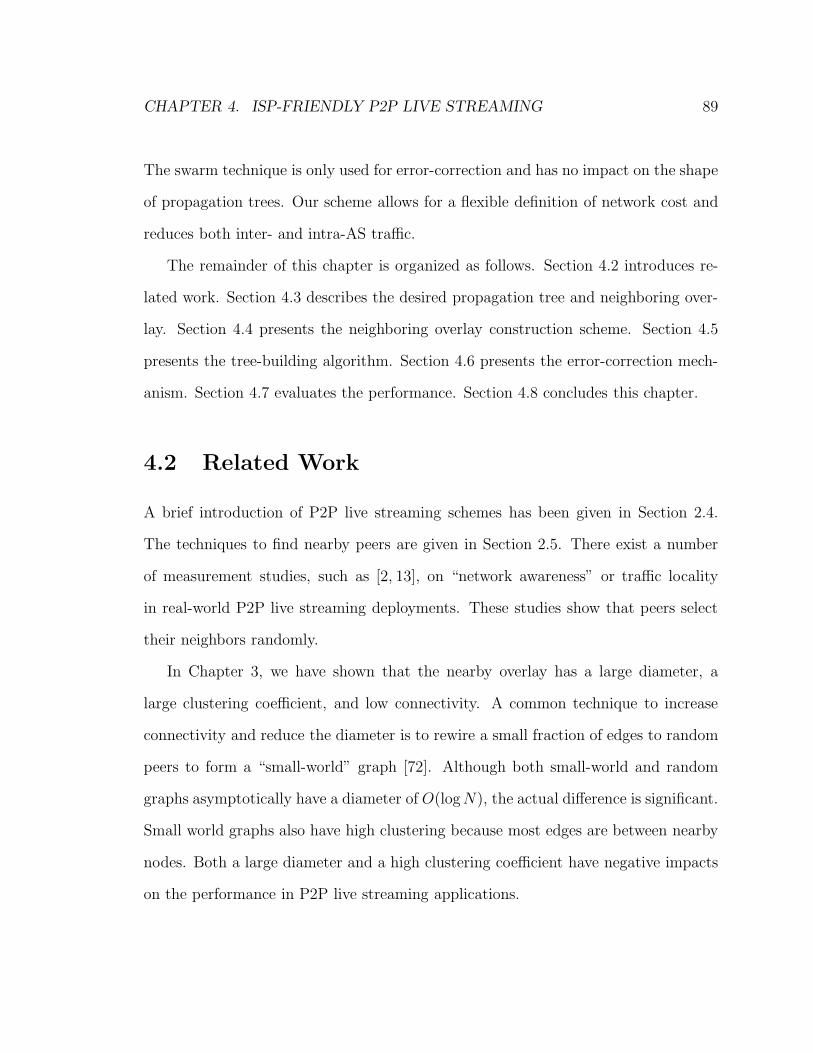
CHAPTER 4. ISP-FRIENDLY P2P LIVE STREAMING 89
The swarm technique is only used for error-correction and has no impact on the shape
of propagation trees. Our scheme allows for a flexible definition of network cost and
reduces both inter- and intra-AS traffic.
The remainder of this chapter is organized as follows. Section 4.2 introduces re-
lated work. Section 4.3 describes the desired propagation tree and neighboring over-
lay. Section 4.4 presents the neighboring overlay construction scheme. Section 4.5
presents the tree-building algorithm. Section 4.6 presents the error-correction mech-
anism. Section 4.7 evaluates the performance. Section 4.8 concludes this chapter.
4.2 Related Work
A brief introduction of P2P live streaming schemes has been given in Section 2.4.
The techniques to find nearby peers are given in Section 2.5. There exist a number
of measurement studies, such as [2, 13], on “network awareness” or traffic locality
in real-world P2P live streaming deployments. These studies show that peers select
their neighbors randomly.
In Chapter 3, we have shown that the nearby overlay has a large diameter, a
large clustering coefficient, and low connectivity. A common technique to increase
connectivity and reduce the diameter is to rewire a small fraction of edges to random
peers to form a “small-world” graph [72]. Although both small-world and random
graphs asymptotically have a diameter of O(logN), the actual difference is significant.
Small world graphs also have high clustering because most edges are between nearby
nodes. Both a large diameter and a high clustering coefficient have negative impacts
on the performance in P2P live streaming applications.
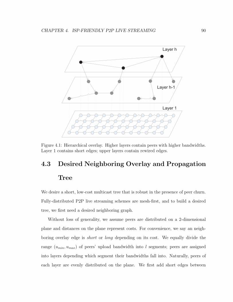
CHAPTER 4. ISP-FRIENDLY P2P LIVE STREAMING 90
Layer h
Layer h-1
Layer 1
Figure 4.1: Hierarchical overlay. Higher layers contain peers with higher bandwidths.Layer 1 contains short edges; upper layers contain rewired edges.
4.3 Desired Neighboring Overlay and Propagation
Tree
We desire a short, low-cost multicast tree that is robust in the presence of peer churn.
Fully-distributed P2P live streaming schemes are mesh-first, and to build a desired
tree, we first need a desired neighboring graph.
Without loss of generality, we assume peers are distributed on a 2-dimensional
plane and distances on the plane represent costs. For convenience, we say an neigh-
boring overlay edge is short or long depending on its cost. We equally divide the
range (umin, umax) of peers’ upload bandwidth into l segments; peers are assigned
into layers depending which segment their bandwidths fall into. Naturally, peers of
each layer are evenly distributed on the plane. We first add short edges between

CHAPTER 4. ISP-FRIENDLY P2P LIVE STREAMING 91
nearby peers then rewire a small fraction of edges to form a hierarchical overlay as
shown in Fig. 4.1. We design the neighboring overlay to have and retain the following
properties in the presence of peer churn. First, high-bandwidth peers are evenly dis-
tributed on the neighboring overlay, i.e., given a layer i and hop count j, the number
of layer i peers in the clique within j hops to any peer x are similar. This property
is necessary to utilize peers’ upload bandwidth. Second, long edges are evenly dis-
tributed on the neighboring overlay and exist between high-bandwidth peers with a
greater probability than between low-bandwidth peers. This applies to both intra-
and inter-layer edges. Third, between peers in the same layer, the probability that an
edge exists is inversely proportional to the distance. The lower the layer, the larger
the impact of distance is.
On the hierarchical overlay, we desire a multicast tree similar to the one shown in
Fig. 4.1. Chunks first go from the video source to a layer l peer, then spread along
layer l edges to every region in the system. At lower layers, chunks spread using
shorter edges. The last few hops, which determine the tree cost, are between nearby
peers. Note that even for peers at high layers, most children are still nearby.
4.4 Overlay Construction
Similar to most P2P live streaming schemes, we use an out-of-band mechanism to find
the video source and the tracker. We assume the existence of a network positioning
scheme (e.g., GNS [46]) such that each peer knows its own network coordinate. Upon
joining the system, peers request a membership table from the tracker and report their
network coordinates and upload bandwidth to the tracker. The tracker maintains a
repository of size Mt. The repository should be large enough to be a representative

CHAPTER 4. ISP-FRIENDLY P2P LIVE STREAMING 92
Table 4.1: System Parameters and Default Values
Notation Comment DefaultMt The size of the tracker’s repository 3000Mp The size of peers’ membership tables 50Tbm Buffer map advertisement interval 1 secTsubs Subscription check interval 1 secTsexp Subscription expire interval 10 secTpull Pull check interval 1 secTlate Margin to decide a chunk is late 1 secTsm Margin to switch parents in TT 1 secTwp Waiting period for parent to relocate on tree 1 secWbuf Buffer size (chunks) 600Wurg Emergency window size in chunks 9Wbbp Number of chunks to buffer before playing 20Wbbs Number of chunks to buffer before skipping 10Lck Chunk size 16 KBRplay Playback rate 64 KB/s
sample of the whole population, i.e., given a peer, the distribution of peers in the
repository is the same as in the whole population with respect to the distance to the
peer and upload bandwidth.
The tracker uses Algorithm 1 to compose a membership table for peer i when
contacted by peer i, and possibly adds peer i to the repository. The tracker first
selects remote peers. Each peer j in the repository is selected with a probability p
p =γ
Mt
e−1
βu−
dκu (4.1)
where γ, β and κ are constant parameters (lines 2–4). The tracker then greedily
selects nearby peers for peer i (lines 5–8). Peer i randomly selects peers from its
membership table to neighbor with. The number of neighbors peer i maintains is
proportional to its upload capacity with a minimum of 4.
Equation 4.1 is designed to simultaneously achieve the properties described in

CHAPTER 4. ISP-FRIENDLY P2P LIVE STREAMING 93
Algorithm 1 The algorithm that the tracker uses to compose a membership tablefor a requesting peer i
Input: rep, the tracker’s repositoryInput: Mp, the size of the membership tableOutput: tab, the membership table for peer i1: tab← φ2: for j in rep do3: if prob(i, j) > random() then4: tab.insert(j)5: rep.sort by cost(i)6: for j in rep do7: if tab.size() ≥Mp then break;8: if j 6∈ tab then tab.insert(j)
Section 4.3. We use an exponential function for two reasons. First, it has the desired
attenuation property. We desire the probability to attenuate sharply when bandwidth
or distance is large and flattens afterwards. Second, the pair-wise distances between
peers on the Internet exhibit an exponential distribution [78]. Using an exponential
function can retain the property on the neighboring overlay. Normalizing the upload
bandwidth and distance as u =(ui−umin)(uj−umin)
(umax−umin)2and d =
dij
dmaxallows for flexible
definitions of cost and bandwidth.
The factor 1Mt
is introduced to ensure that the number of rewired edges in the
neighboring overlay is independent from the size of the tracker’s repository. Parameter
γ controls the fraction of rewired edges over the membership table size; a larger γ
results in a larger fraction of rewired edges. The factor e−1
βu controls the number of
intra- and inter-layer edges between high-bandwidth peers. The factor e−d
κu ensures
that (1) at any layer, the probability that an edge exists between two peers is inversely
proportional to their distance, and (2) with lower bandwidth, distance has a larger
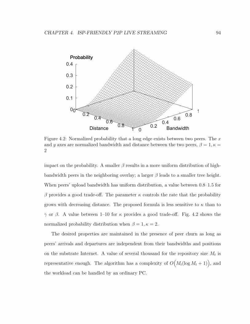
CHAPTER 4. ISP-FRIENDLY P2P LIVE STREAMING 94
BandwidthDistance
0
0.1
0.2
0.3
0.4
Probability
0 0.2
0.4 0.6
0.8 1 0
0.2 0.4
0.6 0.8
1
Probability
Figure 4.2: Normalized probability that a long edge exists between two peers. The xand y axes are normalized bandwidth and distance between the two peers, β = 1, κ =2
impact on the probability. A smaller β results in a more uniform distribution of high-
bandwidth peers in the neighboring overlay; a larger β leads to a smaller tree height.
When peers’ upload bandwidth has uniform distribution, a value between 0.8–1.5 for
β provides a good trade-off. The parameter κ controls the rate that the probability
grows with decreasing distance. The proposed formula is less sensitive to κ than to
γ or β. A value between 1–10 for κ provides a good trade-off. Fig. 4.2 shows the
normalized probability distribution when β = 1, κ = 2.
The desired properties are maintained in the presence of peer churn as long as
peers’ arrivals and departures are independent from their bandwidths and positions
on the substrate Internet. A value of several thousand for the repository size Mt is
representative enough. The algorithm has a complexity of O(
Mt(logMt + 1))
, and
the workload can be handled by an ordinary PC.
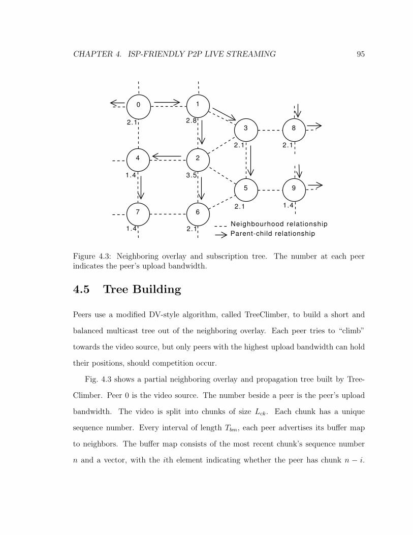
CHAPTER 4. ISP-FRIENDLY P2P LIVE STREAMING 95
0
2
3
4
1
67
5
2.1 2.8
1.4
1.4 3.5
2.1
2.1
2.1
8
9
2.1
1.4
Neighbourhood relationship
Parent-child relationship
Figure 4.3: Neighboring overlay and subscription tree. The number at each peerindicates the peer’s upload bandwidth.
4.5 Tree Building
Peers use a modified DV-style algorithm, called TreeClimber, to build a short and
balanced multicast tree out of the neighboring overlay. Each peer tries to “climb”
towards the video source, but only peers with the highest upload bandwidth can hold
their positions, should competition occur.
Fig. 4.3 shows a partial neighboring overlay and propagation tree built by Tree-
Climber. Peer 0 is the video source. The number beside a peer is the peer’s upload
bandwidth. The video is split into chunks of size Lck. Each chunk has a unique
sequence number. Every interval of length Tbm, each peer advertises its buffer map
to neighbors. The buffer map consists of the most recent chunk’s sequence number
n and a vector, with the ith element indicating whether the peer has chunk n − i.

CHAPTER 4. ISP-FRIENDLY P2P LIVE STREAMING 96
The buffer map message also contains a tree-hops field, which is the number of hops
from the peer to the video source along the subscription tree. If the peer is not on
the subscription tree, its tree-hops is set to the maximum value of 128.
4.5.1 Determining Parent–Child Relationships
Algorithm 2 The algorithm that a peer uses to select its parent
Input: neighbors, the neighbor listOutput: The new parent1: cp← φ2: neighbors.sort by hops()3: h← neighbors.front().hops4: for i in neighbors do5: if i.hops 6= h then break6: if i is the current parent then return i7: if i is not a child then cp.insert(i)8: return cp.at(random(cp.size())
Every interval of length Tsubs, a peer checks whether to switch parents in order to
reduce its tree-hops to the video source. Algorithm 2 shows the greedy algorithm that
a peer uses to select its parent. Neighbors are ranked according to their tree-hops,
and the neighbors with the lowest tree-hops are candidate parents (lines 1–5). A peer
prefers its current parent to reduce parent switches (line 6). However, if its current
parent is not a candidate parent, the peer will randomly select one from the candidate
parents (line 8). To reduce the occurrence of loops, a peer does not select its child
as the new parent (line 7). If the newly selected parent is not the current parent,
the peer will send a subscription request, together with its own upload capacity, to
the new parent immediately. Otherwise, the peer will send a subscription request
to its current parent only when the last subscription expires, i.e., the peer sends

CHAPTER 4. ISP-FRIENDLY P2P LIVE STREAMING 97
subscription requests to its current parent every interval of length Tsexp to keep its
status as a child.
Algorithm 3 The algorithm that a peer uses to handle subscription requests frompeer s
1: if s is child or has spare bandwidth() then2: send(s, ACCEPT )3: else4: d← calc disown target(s)5: if d 6= s then6: send(s, ACCEPT )7: send(d,DISOWN)8: else send(s, REJECT )
Algorithm 3 shows the algorithm that peers use to handle subscription requests.
Peers employ the CAC and preemption mechanisms. A peer divides its upload band-
width into push and pull bandwidths, and accepts children if it has spare push band-
width (lines 1–2). If a peer receives subscription requests from more than one peer,
it accepts the peer with the largest upload bandwidth. The requesting peers’ upload
bandwidth is carried in the requests. A peer will preempt a child if it receives sub-
scription requests from neighbors with higher upload bandwidth (lines 4–8). Suppose
a low upload bandwidth peer l sends a request to peer t earlier and becomes a child.
Then peer t receives a request from a high upload bandwidth peer h but has no spare
push bandwidth. Peer t will accept peer h and disown the child with the lowest up-
load bandwidth. In Fig. 4.3, if peer 4 arrives earlier than peer 1 and attaches to peer
0, peer 1 can preempt peer 4.
When parent y of peer x leaves, peer x attempts to find a new parent immediately.
However, when peer x finds its parent y has lost its parent z, peer x will wait for a
period of length Twp for y to rejoin the subscription tree before searching for a new

CHAPTER 4. ISP-FRIENDLY P2P LIVE STREAMING 98
parent. In Fig. 4.3, if peer 1 leaves, peers 2 and 3 start searching for a new parent
immediately but peers 4, 5, and 6 will wait.
We use tree-hops, the hops of the path from a peer to the video source along the
subscription tree, rather than hops of the shortest path of the neighboring overlay
used by traditional DV protocols. DV protocols require that each node on the neigh-
boring overlay is capable of accepting d− 1 children, where d is the node’s degree on
the neighboring overlay. This requirement is not practical in a P2P live streaming sys-
tem, where peers have limited upload bandwidth. When peers have sufficient upload
bandwidth, our algorithm builds a MST on the neighboring overlay. When peers are
short of upload bandwidth, our algorithm provides a heuristic to the DBMST prob-
lem. In Fig. 4.3, peer 4’s hop count is 1 in the MST and 3 in the DBMST. Note that
the DBMST problem is NP-hard [63].
4.5.2 Avoiding Forwarding Loops and Duplicated Chunks
Much of the complexity of a routing protocol, whether it is a unicast routing protocol
or a multicast routing protocol, comes from the prevention of forwarding loops. For
example, the routing information protocol (RIP) [44] uses split-horizon with poisoned
reverse while the border gateway protocol (BGP) [57] appends the path information
to routing messages. Even a small number of forwarding loops are disastrous because
packets will circle in the loop until their time-to-live field expires. In P2P live stream-
ing systems, every chunk has a unique sequence number. Peers can ignore received
duplicated chunks, and send a chunk to a child only once to stop a chunk from circling
in a loop. Therefore loops can be tolerated if their frequency can be kept at a low
level.

CHAPTER 4. ISP-FRIENDLY P2P LIVE STREAMING 99
Loops are caused by peer churn and asynchronous operations of peers. In Fig. 4.3,
if peer 1 leaves and peer 3 detects peer 1’s departure earlier than peer 2, peer 3 requests
peer 2 to be a parent. When peer 2 detects the departure of peer 1, it requests peer
5 to be a parent. Thus, peers 2, 3, and 5 form a loop. Several factors in TreeClimber
help to keep the occurrence of loops at a low level: the greedy algorithm that a peer
uses to select its parent, an interval of one second that tree-hops are advertised, and
a minimum of four neighbors a peer has. In Fig. 4.3, peer 3 will find peer 8 to be a
better parent within several buffer map advertisement intervals should loop between
peers 2, 3, and 5 occur.
TreeClimber uses a simple strategy to stop chunks from circling in a loop. A peer
pushes a chunk to its children only upon receiving the chunk for the first time. A
peer c can specify from which sequence number n it wishes to receive chunks in the
subscription request to peer p. Peer p will push chunks whose sequence number is
larger than n. However, if peer p has proceeded to a position later than n when
receiving the request, it will not push the chunks ahead of n to peer c. Peer c must
explicitly pull those chunks.
4.5.3 Fast Tree Repairing
IP multicast protocols and early tree-based schemes that aim to replace IP multicast
are slow to repair the multicast tree when nodes leave. Because these schemes cannot
assume packets arrive with a constant rate, peers cannot detect the failures of parents
by monitoring packet arrivals. In order to avoid forwarding loops, peers cannot have
backup parents; they have to wait until the routing table stabilizes to find a new
parent.
CHAPTER 4. ISP-FRIENDLY P2P LIVE STREAMING 100
Recent P2P live streaming applications only target applications that have near-
constant streaming rate. A peer monitors packet arrivals from its parent and can
quickly detect the failure of its parent. Each packet has a unique sequence number,
and forwarding loops can be avoided at the forwarding plane. These are the same in
data-driven and network-driven schemes.
In data-driven tree-based schemes, a peer knows the buffer maps and spare upload
bandwidth of its neighbors and can quickly pick a new parent should its current parent
leave. In network-driven tree-based schemes, if a peer could pick a new parent as fast
as in data-driven schemes, tree-repairing would be equally fast. In TreeClimber, the
tree-hop information of neighbors is carried in buffer map messages, and hence tree-
repairing is as fast in TreeClimber as in data-driven schemes.
4.6 Error-Correction
A peer has to pull chunks for two reasons: Internet link errors and peer churn. A
chunk may get lost during transmission because of Internet link errors. When a peer’s
parent leaves, the peer needs some time to find a new parent. When it find a new
parent, the parent may proceed to a later position and will not push the chunks it
has already pushed to the new child. We use the swarm technique as a multi-point
re-transmission mechanism to pull missing chunks. Unlike in data-driven schemes
where the swarm technique is used for both tree-building and error correction, the
swarm technique is used only for error-correction in our scheme.
Each peer maintains a buffer of size Wbuf to hold recently received chunks. Peers
have a small emergency window of size Wurg, consisting of chunks approaching play-
back deadlines. Every interval of length Tpull, a peer requests all the missing chunks

CHAPTER 4. ISP-FRIENDLY P2P LIVE STREAMING 101
in the emergency window. The targets of requests are randomly chosen from neigh-
bors. After examining the simulation results, we decided to eliminate the swarming
window. In TreeClimber, the push bandwidth is guaranteed by the CAC scheme; pull
operations use the residual bandwidth. Upon receiving a pull request, a peer replies
with the chunk if it has spare upload bandwidth; otherwise, it rejects the request.
Each peer maintains a sliding window of late chunks. A peer monitors chunk
arrivals to estimate arrival times of future chunks. A chunk is considered late if it has
not arrived until an interval of Tlate after its due time. Every interval of length Tpull, a
peer pulls all the late chunks in order of urgency (with respect to playback deadlines).
Peers advertise their residual bandwidth to neighbors in buffer map messages. We
use an innovative pull mechanism that has a high success rate of fetching them.
The scheduling algorithm attempts to maximize the number of chunks pulled while
keeping load balanced among neighbors.
Algorithm 4 shows the algorithm that a peer uses to select the neighbors to pull
chunks from. A peer knows the chunks each neighbor has and the residual bandwidth
of the neighbor at the neighbor’s last advertisement time. A peer first, for each chunk,
calculate the number of neighbors that have the chunk. Starting with the chunks that
are only available at one neighbor, the peer assigns a pulling target to each chunk.
If a chunk is available at only one neighbor, that neighbor is selected. If a chunk is
available at more than one neighbor, the peer selects one randomly.
4.7 Performance Evaluation
In this section, we compare the performance of TreeClimber with the typical tree-
based scheme (called TT) introduced in Chapter 2, and compare the performance of

CHAPTER 4. ISP-FRIENDLY P2P LIVE STREAMING 102
Algorithm 4 The algorithm that a peer uses to select neighbors to pull missingchunks from
Input: chunks[M ], the chunks to be pulledInput: res bw[N ], the residual bandwidth of neighborsInput: avail[M ][N ], a matrix denoting which chunks are available at which neighborsOutput: out, a list of (c,t) pairs denoting which chunks to pull from which neighbors1: for i in [0,M) do2: avai nei cnt[i] = num avail nei(chunks[i])3: n← 14: while n ≤ N do5: m← 16: while m ≤M do7: if avail nei cnt[m] == n then8: k ← rand sel nei(chunks[m])9: out.push back(m, k)
10: avail nei cnt[m]← −111: update residual bw(k)12: if res bw[k] < 1 then13: update avail matrix()14: n← 115: m← 016: break17: else m+ +18: else m+ +19: if m == M then n+ +

CHAPTER 4. ISP-FRIENDLY P2P LIVE STREAMING 103
TreeClimber on the hierarchical overlay with that on the random overlay and small-
world overlay.1
4.7.1 Simulation Setting
We use the same simulation setting as described in Section 3.4 except for the following.
In TreeClimber, a peer advertises its tree-hops in buffer map messages to neighbors
every interval of length Tbm, and if a neighbor has fewer tree-hops than its current
parent, it will request the neighbor to be the new parent. A late-arriving peer is
to preempt an earlier peer if its bandwidth has a margin of 1. We compare three
neighboring overlays: random overlay, small-world overlay, and hierarchical overlay
(abbreviated as RO, SO, and HO hereafter); the latter two have the same fraction of
rewired edges (about 4%).
4.7.2 TreeClimber vs. Typical Tree-Based (TT) Scheme
We report the results of using the bandwidth setting of U(0, 6). The results of using
the bandwidth setting of U(1, 4) and U(1, 9) lead to the same conclusion.
Fig. 4.4 shows the normalized propagation tree cost of TreeClimber on the hier-
archical overlay when the bandwidth setting is U(0, 6) and compares it with that of
TT. TreeClimber has a slightly higher cost, indicating that the long edges are more
heavily used in TreeClimber. This is expected because we want packets to quickly
propagate from the video source using these long edges.
1Hierarchical overlays also have the small-world graph properties (i.e., a high clustering coefficientand a small diameter). In this thesis, we call overlays where a small fraction of edges are rewiredrandomly small-world overlays, and call overlays where a small fraction of edges are rewired accordingto Equation 4.1 hierarchical overlays.

CHAPTER 4. ISP-FRIENDLY P2P LIVE STREAMING 104
0
0.2
0.4
0.6
0.8
1
0 1 2 3 4 5 6 7 8 9
No
rma
lize
d P
rop
ag
atio
n T
ree
Co
st
Topology Number
TTTC
Figure 4.4: Normalized propagation tree cost of the hierarchical overlay when thebandwidth setting is U(0, 6).
6
8
10
12
14
16
18
0 1 2 3 4 5 6 7 8 9
Pro
pa
ga
tio
n T
ree
He
igh
t
Topology Number
TTTC
Figure 4.5: Average propagation tree height on the hierarchical overlay when thebandwidth setting is U(0, 6).

CHAPTER 4. ISP-FRIENDLY P2P LIVE STREAMING 105
0
0.2
0.4
0.6
0.8
1
5 6 7 8 9 10
Fra
ctio
n o
f P
ee
rs C
DF
Playback Delay (sec)
TTTC
Figure 4.6: Playback delay CDF on the hierarchical overlay when the bandwidthsetting is U(0, 6).
Fig. 4.5 shows the propagation tree height of TreeClimber on the hierarchical
overlay when the bandwidth setting is U(0, 6) and compares it with that of TT.
TreeClimber has a significantly lower tree height than TT, as expected.
Fig. 4.6 shows the playback delay of TreeClimber on the hierarchical overlay when
the bandwidth setting is U(0, 6) and compares it with that of TT. Although Tree-
Climber has a lower tree height, its playback delays are similar to TT. This is because
in TreeClimber, the inner nodes on the tree have more children and hence longer queu-
ing delays.
Fig. 4.7 shows the delivery-rate-user-ratio of TreeClimber on the hierarchical over-
lay when the bandwidth setting is U(0, 6) and compares it with that of TT. More
peers received all the chunks in TreeClimber than in TT. This is because TreeClimber
has a higher success rate in pulling chunks due to the propagation tree shape. A peer
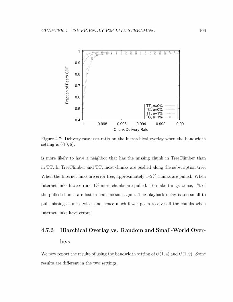
CHAPTER 4. ISP-FRIENDLY P2P LIVE STREAMING 106
0.4
0.5
0.6
0.7
0.8
0.9
1
0.99 0.992 0.994 0.996 0.998 1
Fra
ctio
n o
f P
ee
rs C
DF
Chunk Delivery Rate
TT, e=0%TC, e=0%TT, e=1%TC, e=1%
Figure 4.7: Delivery-rate-user-ratio on the hierarchical overlay when the bandwidthsetting is U(0, 6).
is more likely to have a neighbor that has the missing chunk in TreeClimber than
in TT. In TreeClimber and TT, most chunks are pushed along the subscription tree.
When the Internet links are error-free, approximately 1–2% chunks are pulled. When
Internet links have errors, 1% more chunks are pulled. To make things worse, 1% of
the pulled chunks are lost in transmission again. The playback delay is too small to
pull missing chunks twice, and hence much fewer peers receive all the chunks when
Internet links have errors.
4.7.3 Hiarchical Overlay vs. Random and Small-World Over-
lays
We now report the results of using the bandwidth setting of U(1, 4) and U(1, 9). Some
results are different in the two settings.
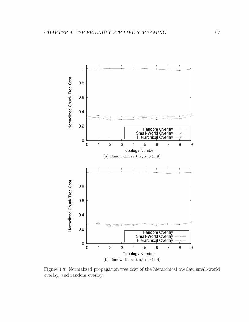
CHAPTER 4. ISP-FRIENDLY P2P LIVE STREAMING 107
0
0.2
0.4
0.6
0.8
1
0 1 2 3 4 5 6 7 8 9
No
rma
lize
d C
hu
nk T
ree
Co
st
Topology Number
Random OverlaySmall-World OverlayHierarchical Overlay
(a) Bandwidth setting is U(1, 9)
0
0.2
0.4
0.6
0.8
1
0 1 2 3 4 5 6 7 8 9
No
rma
lize
d C
hu
nk T
ree
Co
st
Topology Number
Random OverlaySmall-World OverlayHierarchical Overlay
(b) Bandwidth setting is U(1, 4)
Figure 4.8: Normalized propagation tree cost of the hierarchical overlay, small-worldoverlay, and random overlay.

CHAPTER 4. ISP-FRIENDLY P2P LIVE STREAMING 108
Table 4.2: Average Propagation Tree and SPT Height
Propagation Tree SPTU(1, 9) U(1, 4) U(1, 9) U(1, 4)
Random Overlay 8.1 14.0 5.0 7.0Small-Wolrd Overlay 11.2 21.4 8.4 11.6Hierarchical Overlay 8.2 16.7 7.1 10.6
Fig. 4.8 compares the normalized propagation tree cost of the hierarchical overlay,
small-world overlay, and random overlay when the bandwidth setting is U(1, 4) and
U(1, 9). Under the loose bandwidth constraints, the propagation tree cost of the
small-world overlay is slightly lower than on the hierarchical overlay. Under the tight
bandwidth constraints, long edges are used less often because peers have fewer choices,
and the propagation tree cost is similar on the small-world overlay and hierarchical
overlay.
Table. 4.2 compares the propagation tree height on the hierarchical overlay, small-
world overlay, and random overlay when the bandwidth setting is U(1, 4) and U(1, 9).
Under loose bandwidth constraints, the propagation tree height is similar on the
hierarchical overlay and on the random overlay, and is lower than on the nearby
overlay. However, under tight bandwidth constraint, the propagation tree height is
lower on the random overlay than on the hierarchical overlay.
To investigate the causes, we assume that each peer has sufficient upload band-
width and compute the SPT rooted at the video source on the three overlays, which
is shown in Table. 4.2. Although the three overlays asymptotically have a diameter of
O(logN), the random overlay actually has a significant smaller diameter, especially
under the tight bandwidth constraints. As a consequence, the propagation tree is
lower on the random overlay. The reason for lower propagation tree height on the
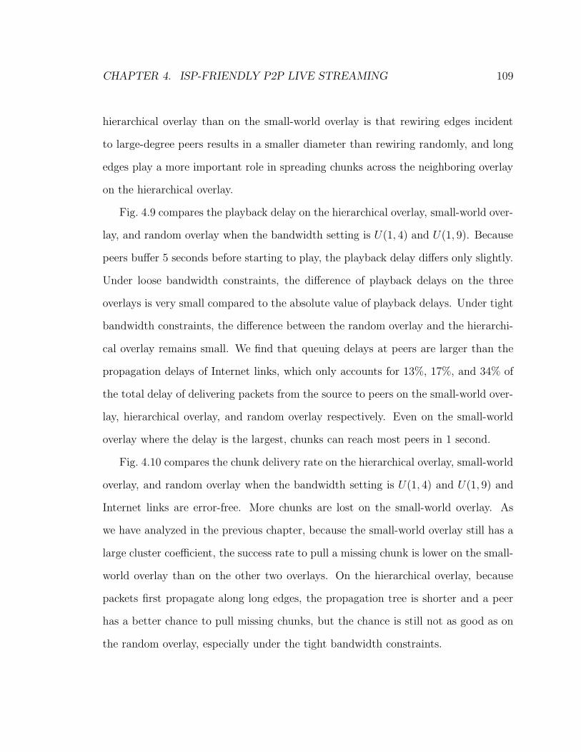
CHAPTER 4. ISP-FRIENDLY P2P LIVE STREAMING 109
hierarchical overlay than on the small-world overlay is that rewiring edges incident
to large-degree peers results in a smaller diameter than rewiring randomly, and long
edges play a more important role in spreading chunks across the neighboring overlay
on the hierarchical overlay.
Fig. 4.9 compares the playback delay on the hierarchical overlay, small-world over-
lay, and random overlay when the bandwidth setting is U(1, 4) and U(1, 9). Because
peers buffer 5 seconds before starting to play, the playback delay differs only slightly.
Under loose bandwidth constraints, the difference of playback delays on the three
overlays is very small compared to the absolute value of playback delays. Under tight
bandwidth constraints, the difference between the random overlay and the hierarchi-
cal overlay remains small. We find that queuing delays at peers are larger than the
propagation delays of Internet links, which only accounts for 13%, 17%, and 34% of
the total delay of delivering packets from the source to peers on the small-world over-
lay, hierarchical overlay, and random overlay respectively. Even on the small-world
overlay where the delay is the largest, chunks can reach most peers in 1 second.
Fig. 4.10 compares the chunk delivery rate on the hierarchical overlay, small-world
overlay, and random overlay when the bandwidth setting is U(1, 4) and U(1, 9) and
Internet links are error-free. More chunks are lost on the small-world overlay. As
we have analyzed in the previous chapter, because the small-world overlay still has a
large cluster coefficient, the success rate to pull a missing chunk is lower on the small-
world overlay than on the other two overlays. On the hierarchical overlay, because
packets first propagate along long edges, the propagation tree is shorter and a peer
has a better chance to pull missing chunks, but the chance is still not as good as on
the random overlay, especially under the tight bandwidth constraints.
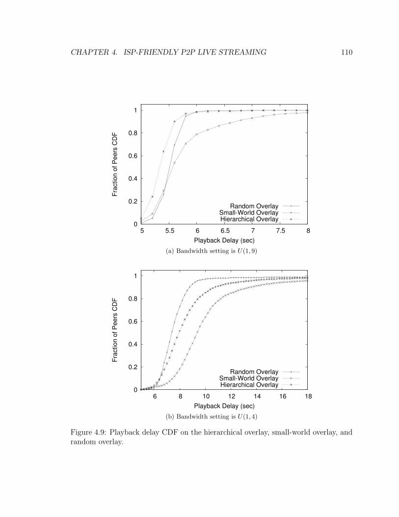
CHAPTER 4. ISP-FRIENDLY P2P LIVE STREAMING 110
0
0.2
0.4
0.6
0.8
1
5 5.5 6 6.5 7 7.5 8
Fra
ctio
n o
f P
ee
rs C
DF
Playback Delay (sec)
Random OverlaySmall-World OverlayHierarchical Overlay
(a) Bandwidth setting is U(1, 9)
0
0.2
0.4
0.6
0.8
1
6 8 10 12 14 16 18
Fra
ctio
n o
f P
ee
rs C
DF
Playback Delay (sec)
Random OverlaySmall-World OverlayHierarchical Overlay
(b) Bandwidth setting is U(1, 4)
Figure 4.9: Playback delay CDF on the hierarchical overlay, small-world overlay, andrandom overlay.
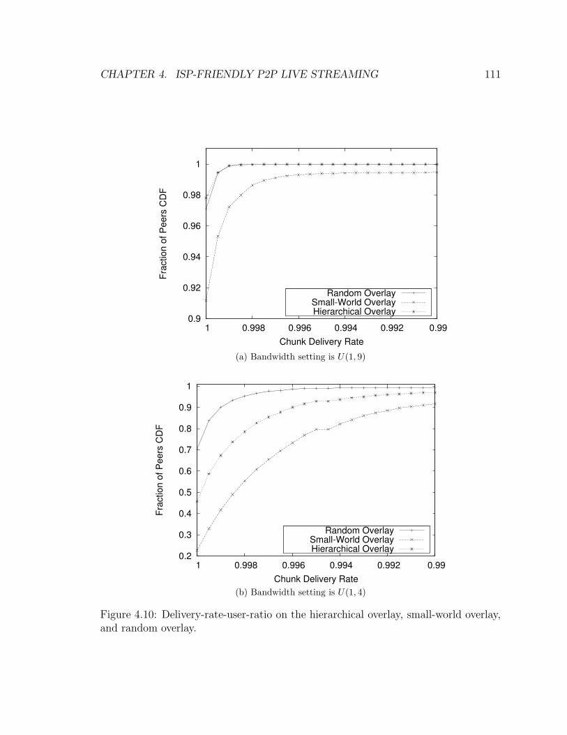
CHAPTER 4. ISP-FRIENDLY P2P LIVE STREAMING 111
0.9
0.92
0.94
0.96
0.98
1
0.99 0.992 0.994 0.996 0.998 1
Fra
ctio
n o
f P
ee
rs C
DF
Chunk Delivery Rate
Random OverlaySmall-World OverlayHierarchical Overlay
(a) Bandwidth setting is U(1, 9)
0.2
0.3
0.4
0.5
0.6
0.7
0.8
0.9
1
0.99 0.992 0.994 0.996 0.998 1
Fra
ctio
n o
f P
ee
rs C
DF
Chunk Delivery Rate
Random OverlaySmall-World OverlayHierarchical Overlay
(b) Bandwidth setting is U(1, 4)
Figure 4.10: Delivery-rate-user-ratio on the hierarchical overlay, small-world overlay,and random overlay.

CHAPTER 4. ISP-FRIENDLY P2P LIVE STREAMING 112
5
6
7
8
9
10
0.02 0.04 0.08 0.16 0.32 0.2
0.3
0.4
0.5
0.6
0.7
Str
etc
h a
nd T
ree H
eig
ht
Percentage of Long Edges
Tree HeightSPT Height
Normalized Tree Cost
Figure 4.11: Impact of fraction of rewired edges on the hierarchical overlay when thebandwidth setting is U(1, 9).
4.7.4 Impact of Long Edges
The fraction of long edges has a great impact on the neighboring overlay. Rewiring
1% of edges to random nodes in a regular graph can reduce the characteristic path
length by 80% [72]. However, in a P2P network, a larger fraction is necessary to
prevent system partitioning in the presence of peer churn. Fig. 4.11 shows the impact
of the fraction of rewired edges on the propagation tree cost and height. The tree
cost is proportional to the fraction but the tree height decreases marginally when
the fraction is larger than 15%. Rewiring 5–10% long edges usually provides a good
trade-off. When peers’ upload bandwidths are larger, a smaller fraction can be used.

CHAPTER 4. ISP-FRIENDLY P2P LIVE STREAMING 113
0.4
0.5
0.6
0.7
0.8
0.9
1
0.99 0.992 0.994 0.996 0.998 1
Fra
ction o
f P
eers
CD
F
Chunk Delivery Rate
4.4% Long Edges, Buffer 5 Sec8.9% Long Edges, Buffer 5 Sec8.9% Long Edges, Buffer 8 Sec
Figure 4.12: Impact of playback delay
4.7.5 Trade-Off Between the Playback Delay and Delivery
Rate
The primary trade-off in pull schemes is between playback delay and video quality.
Buffering more chunks before playing improves the chunk delivery rate. In our scheme,
1–2% of chunks are pulled (i.e., obtained by the swarm technique). The delivery rate
is determined by the success rate to pull missing chunks. Although a longer buffering
delay translates into a longer playback delay, the fraction of users receiving all the
chunks becomes higher. Fig. 4.12 shows the trade-off between the playback delay and
chunk delivery rate. At a buffering time of 5 seconds, the fraction of such users is
63%, as opposed to 92% when the buffering time is 8 seconds. We remark that further
increasing the buffering time only marginally improves chunk delivery. Fig. 4.12 also
shows that, when the neighboring overlay has fewer edges, more edges should be
rewired. New chunks can spread faster and reach even distribution in the system in

CHAPTER 4. ISP-FRIENDLY P2P LIVE STREAMING 114
a shorter time.
4.8 Summary
Simply applying the neighbor-with-nearby-peers strategy to reduce network traffic
in P2P video live streaming applications may cause more lost video chunks, espe-
cially in data-driven tree-based schemes. In this chapter, we proposed a hierarchical
overlay scheme and a network-driven tree-based scheme, called TreeClimber, to mit-
igate these drawbacks. Most edges on the hierarchical overlay are short, but a small
fraction of long edges are added and used by the DV-style tree-building algorithm
to quickly distribute packets from the video source to each part of the neighboring
overlay. We compared our scheme with the typical tree-based scheme described in the
previous chapter and the random and small-world overlays. Simulation results show
our scheme outperforms the typical data-driven tree-based scheme and the hierarchi-
cal overlay outperforms the small-world overlay. More users received all the chunks
in TreeClimber than in the typical data-driven tree-based scheme. The network cost
of the hierarchical overlay is only 13
of that on the random overlay, and the chunk
delivery rate is close to that on the random overlay under loose upload bandwidth
constraints.

Chapter 5
FEC Performance in Interactive
Streaming
5.1 Introduction
The past few years have witnessed significant growth of multimedia communication
applications on the Internet. These applications can only tolerate a few hundred
milliseconds of delay at best, and unlike audio communication applications, they
are sensitive to packet loss. Forward error correction (FEC) codes are the preferred
error correction technique for multimedia communication applications, and the Reed
Solomon (RS) codes are the most widely used FEC codes. FEC can be classified into
systematic FEC and non-systematic FEC. Codes that include the original packets in
the output are systematic and codes that do not are non-systematic. With systematic
FEC codes, after FEC correction, the packet loss ratio is lower and the packet losses
are less bursty when compared to non-systematic FEC codes. Both properties are
beneficial to video quality.
115
CHAPTER 5. FEC PERFORMANCE IN INTERACTIVE STREAMING 116
FEC is effective in correcting sporadic packet losses of a communication channel.
However, studies [50,76] show that packet losses often occur in bursts of consecutive
losses on Internet links. This burstiness of packet losses is usually modeled using the
Gilbert channel model [23] or its variants. The performance of non-systematic RS
codes on a single Gilbert channel is studied in [17], and the performance of systematic
RS codes on a 2-state Markov chain channel, which is a widely used variant of the
Gilbert channel, is studied in [21]. Results show that the performance of FEC is
greatly jeopardized by the burstiness of packet losses of a communication channel.
A number of studies [6, 18, 34, 80] propose that a sender uses multiple paths to
send packets to a receiver in a round-robin fashion to combat bursty packet losses of
Internet links. These schemes assume the existence of multiple disjoint paths, which
are stable during the communication process. Multimedia communication applica-
tions typically use a set of intermediate nodes to establish multiple overlay paths
between two communication parties. The most feasible option for these intermediate
nodes is to use other users in the application, i.e., users are organized into a peer-to-
peer (P2P) network and a set of peers are used as the intermediate nodes between
two communication parties. Indeed, many communication applications, most notably
Skype [100], use P2P networks. However, in a practical P2P network, peers may leave
abruptly at any time. Using dynamic peers as intermediate nodes for path diversity
may cause additional lost packets when these peers leave. Besides, two paths that
are disjoint from the perspective of the overlay may not be disjoint from the perspec-
tive of the substrate Internet1. Consequently, enough disjoint substrate paths may
not exist between two communication parties or even no disjoint paths at all. It is
1In this thesis, unless otherwise specified, we distinguish whether two paths are disjoint or notfrom the perspective of the substrate Internet.

CHAPTER 5. FEC PERFORMANCE IN INTERACTIVE STREAMING 117
unknown whether using peers to establish multiple overlay paths can really improve
FEC performance or under what conditions the performance can be improved, and
how much improvement is possible.
In this chapter, we study the performance of systematic FEC codes when using
dynamic peers to provide multiple one-hop overlay paths between two communication
parties, and compare this with the post-FEC loss ratio when a single direct Internet
path is used. Since a sender may not be able to find enough disjoint substrate paths
to a receiver, we study the situations where the sender uses a limited number of
disjoint paths, or a large number of non-disjoint paths, in addition to the situation
when the sender is able to find enough disjoint paths. We model Internet links, with
or without peers as intermediate hops, using discrete-time Markov chains. Unlike
other studies that either use non-systematic FEC codes2 or compute approximate
results with heuristic methods, we use systematic FEC codes and compute exact
numerical results. We also use simulation to investigate FEC performance in two
practical situations: where Internet paths have heterogeneous loss ratios and burst
lengths, and where a sender lacks the knowledge of which paths are disjoint and
sends packets via a set of random paths. We find that although using dynamic peers
for path diversity often results in a lower post-FEC loss ratio, conditions do apply.
The interplay of a number of factors—the Internet links’ loss ratio and burst length,
the number of disjoint channels, the lifespans of peers, the time necessary to detect
peers’ departures, and the coding parameters—determines the performance of FEC.
Guidelines exist, but no simple formula exists to determine whether the use of peers
for path diversity can be justified. For example, using peers to establish multiple
2We have developed methods to compute the post-FEC loss ratio for both systematic and non-systematic codes. In this chapter, we focus on systematic codes because they can achieve bettervideo quality. Please refer to Appendix A for non-systematic codes.
CHAPTER 5. FEC PERFORMANCE IN INTERACTIVE STREAMING 118
paths will not reduce the post-FEC loss ratio more than using only the direct path
when Internet links have a low packet loss ratio or certain coding parameters are
used. An application should carefully evaluate the gain of FEC performance before
using peers for path diversity or deciding on coding parameters.
The remainder of this chapter is organized as follows. Section 5.2 introduces re-
lated work. Section 5.3 describes how to use peers to establish multiple paths between
two communication parties. Section 5.4 analyzes the post-FEC packet loss ratio when
a single channel is used; the results serve as the benchmark. Sections 5.5, 5.6, and 5.7
analyze the post-FEC packet loss ratio in three situations—where there exist suffi-
cient disjoint channels, a limited number of disjoint channels, and a large number
of non-disjoint channels—and present relevant models. Section 5.8 investigates FEC
performance where a sender uses heterogeneous Internet links or lacks the knowledge
of which paths are disjoint by simulation. Section 5.9 concludes this chapter.
5.2 Related Work
Elliott [17] pioneered the study of FEC performance in the context of telephone net-
works. He used the Gilbert channel model [23] and introduced two general approaches—
a recursive approach and a generating function approach—to compute the probability
that m errors occur in a block of n bits after FEC correction on a single channel.
However, the approaches in [17] do not distinguish the loss of original bits and FEC
bits and hence only apply to non-systematic FEC codes. Frossard [21] uses a 2-
state Markov chain channel model and systematic FEC codes. He uses the recursive
approach to compute the post-FEC packet loss ratio and burst length for a single
CHAPTER 5. FEC PERFORMANCE IN INTERACTIVE STREAMING 119
channel. However, we find his method to be inaccurate3. Li et al. [36] use the same
2-state Markov chain channel model and systematic RS(n, k) codes as [21]. They
assume that a group of pictures (GOP) has g blocks and a block has k packets. They
use the distortion model in [35] to evaluate video distortion by computing the prob-
ability of each possible sequence of gk packets of a GOP. Yu et al. [77] assume that
packet losses are caused by a single bottleneck node. A number of senders encode
packets with a non-systematic FEC code and send encoded packets to their respec-
tive receivers via the bottleneck node, which is modeled as a G/M/1/K queue. The
post-FEC packet loss ratio is computed using a recursive method.
The general idea of using multiple paths to combat bursty loss has been explored
in a number of research efforts [6,18,34,80]. Zhang et al. [80] use a Bernoulli channel
model (i.e., packet losses are independent and hence not bursty) and non-systematic
FEC codes. They define video distortion as the mean square error of the original
packets and the decoded packets (after FEC correction) of an FEC block, and compare
the distortion when using multiple paths with FEC, a single path with FEC, and
multiple paths without FEC. Begen et al. [6] use a 2-state Markov chain channel
model (same as [21]) and multiple description coding (MDC). They formulate a path
selection problem to maximize video quality. Fashandi et al. [18] use an s-state
continuous-time Markov chain channel model. In each state i, the chain has a rate
of pi,i+1 to go to state i + 1 and a rate pi,0 to go to state 0 (except at the state
s − 1 it only has a rate ps−1,0 to go to state 0). Each path i has a bandwidth of Bi
packets per time unit. The authors use non-systematic RS(n, k) codes and formulate
an optimization problem to find the streaming rates (b1, b2, . . . , bN) allocated to the
N paths that minimize the post-FEC loss ratio under the conditions∑Ni=1 bi = n and
3We use RS(3, 2) as an example to show Frossard’s method is inaccurate in Appendix B.
CHAPTER 5. FEC PERFORMANCE IN INTERACTIVE STREAMING 120
∀i ∈ (1, N), bi ≤ Bi.
The work of Li et al. [34] is closest to ours. They use systematic FEC codes and
N disjoint Internet paths, which are established by the use of an overlay network and
the traceroute tool. They use an s-state discrete-time Markov chain channel model.
In each state i, the chain has a probability of pi,i+1 to go to state i+ 1 (except at the
state s−1 it has a probability of ps−1,s−1 to go to itself) and a probability of pi,0 to go
to state 0. They use a heuristic method to estimate the post-FEC loss ratio, which
is based on two assumptions: (1) both the size n of FEC blocks and the number N
of disjoint paths are large, and (2) the loss of original packets and FEC packets of an
FEC block are independent and have a normal distribution. Both assumptions are
not applicable in multimedia communication applications.
5.3 Network Model
In this section, we introduce how a multimedia communication application can or-
ganize peers into a P2P network and use peers to establish multiple one-hop overlay
paths between two communication parties, as well as the three possible situations of
path diversity. We also give a brief introduction to systematic RS codes.
5.3.1 P2P Network Model
A P2P network is a distributed system in which a transient population of peers self-
organize into an overlay network on top of the substrate Internet to share computing
power, storage, and communication bandwidth [3]. A new peer acquires its initial

CHAPTER 5. FEC PERFORMANCE IN INTERACTIVE STREAMING 121
Figure 5.1: Network model. The sender encodes k = 7 original packets into an FECblock of size n = 8 by appending an FEC packet and sends encoded packets via Nchannels in a round-robin fashion. The receiver can reproduce all the original packetsif no more than n− k = 1 packet is lost in transmission.
membership table, which consists of peers in the P2P network, by contacting a well-
known tracker or by contacting some peers already in the system. A peer maintains
the size of its membership table within in a certain range (e.g., between 50 and 100),
and contacts the tracker or peers in its membership table for more peers if the table
size drops below this range. To reduce communication overhead, a peer does not
exchange keep-alive messages with peers in its membership table, or it uses a large
interval (e.g., one keep-alive message every 30 minutes). Therefore, a peer may not
know that some peers in its membership table have already left.
Two peers can communicate using the direct path (i.e., the shortest IP unicast
path between them) or via a number of care-of (CO) peers to achieve path diversity
(see Fig. 5.1). We call a path without a CO peer a unicast channel and a path with
a CO peer a CO channel. When a sender and a receiver initiate a communication
session, they try to find CO peers that are located between them on the Internet
(i.e., the sum of propagation delays from a CO peer to the sender and the receiver
is close to the propagation delay between the sender and the receiver). There are
many schemes for the sender and receiver to find these peers in a distributed P2P

CHAPTER 5. FEC PERFORMANCE IN INTERACTIVE STREAMING 122
network. For example, they can use virtual network position schemes such as [15] and
a center server that maintains all the peers’ network positions or distributed position-
based routing schemes [24] to do so. The sender specifies the destination peer in a
packet and sends the packet to one of the CO peers, which immediately forwards the
packet to the destination peer. (We only discuss one direction of the communication;
the other direction is the same.) When multiple channels exist between a sender
and a receiver, the sender spreads packets across all the channels in a round-robin
fashion. Assuming there are N channels, the sender will send the (iN + j)-th packet,
i = 0, 1, . . ., via the j-th channel.
In a P2P network, peer departures (and arrivals) are typically modeled as a Poisson
process, which is equivalent to a Bernoulli process in discrete time. An existing CO
peer has a probability of 0 ≤ d ≤ 1 to leave the P2P network in any time unit.
(Multimedia communication applications typically have a near-constant bit rate, and
we denote the interval between two consecutive packets to be one time unit.) The
sender and receiver stay in the system for the whole communication session, i.e., they
have a probability of 0 to leave. The sender exchanges keep-alive messages with CO
peers periodically; it takes s time units for the sender to detect the departure of a
CO peer. Parameters are listed in Table 5.1.
5.3.2 Path Diversity
The Internet routes packets to their destination IP addresses via the shortest IP
paths. When a sender sends packets to a receiver via CO peers, from the perspective
of the substrate Internet, the IP paths between the sender and the receiver are the
two shortest path trees (SPTs) that root at the sender and the receiver respectively
CHAPTER 5. FEC PERFORMANCE IN INTERACTIVE STREAMING 123
Table 5.1: Parameters
Parameter Commentn, k The number of total packets and original packets in an FEC block
with RS(n, k) codingN The number of disjoint pathsd The probability that a peer leaves in any time units The time the sender takes to detect a CO peer’s departurep, q The parameters of the 2-state and (s+ 2)-state Markov chainse, (ec) The packet loss ratio of unicast (or CO) channelsl, (lc) The average burst length of unicast (or CO) channels
with CO peers as leaves.
Internet users typically connect to a point-of-presence (PoP) of an ISP, or several
PoPs for higher reliability, to connect to the Internet. For example, residential users
usually connect to a single PoP, possibly via a home network; campus users usually
have a local area network (LAN) and connect to several PoPs. Beyond PoPs, the
Internet core is a rich mesh network. Fig. 5.2 shows the number of independent IP
addresses at each hop from a residential user and a campus user (both located in
North America) to the 200 most popular websites. The list of websites is obtained
from Alexa [91]. We extracted their addresses and removed redundant addresses, and
used the traceroute to obtain the Internet paths to these addresses. The second hop
of the residential user is a broadband remote access server (BRAS) of the ISP; there
are 36 unique IP addresses beyond the BRAS. The fourth hop of the campus user
includes two exit points of the campus network, and each exit point connects to two
PoPs of ISPs. Our observations of path diversity agree with [26], which uses both
popular websites and hosts in P2P networks.
Since there may not be enough disjoint paths between a sender and a receiver,
communication applications may choose to use only disjoint paths, or to use a large
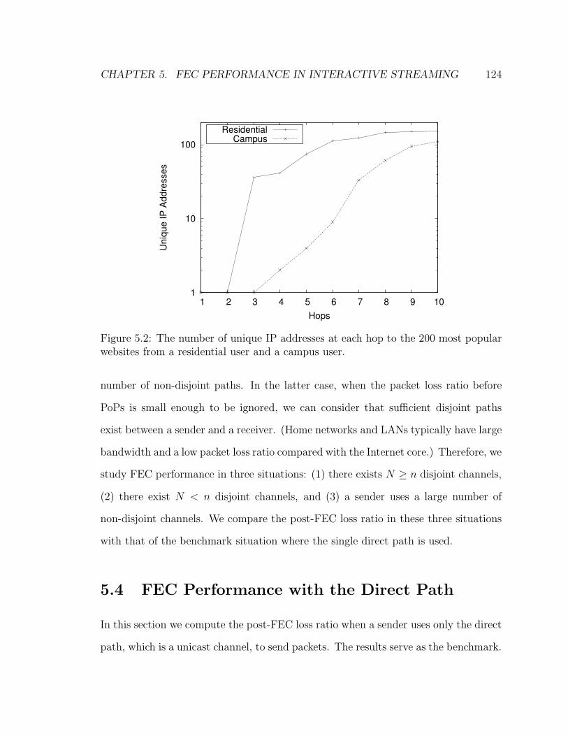
CHAPTER 5. FEC PERFORMANCE IN INTERACTIVE STREAMING 124
1
10
100
1 2 3 4 5 6 7 8 9 10
Un
iqu
e I
P A
dd
resse
s
Hops
ResidentialCampus
Figure 5.2: The number of unique IP addresses at each hop to the 200 most popularwebsites from a residential user and a campus user.
number of non-disjoint paths. In the latter case, when the packet loss ratio before
PoPs is small enough to be ignored, we can consider that sufficient disjoint paths
exist between a sender and a receiver. (Home networks and LANs typically have large
bandwidth and a low packet loss ratio compared with the Internet core.) Therefore, we
study FEC performance in three situations: (1) there exists N ≥ n disjoint channels,
(2) there exist N < n disjoint channels, and (3) a sender uses a large number of
non-disjoint channels. We compare the post-FEC loss ratio in these three situations
with that of the benchmark situation where the single direct path is used.
5.4 FEC Performance with the Direct Path
In this section we compute the post-FEC loss ratio when a sender uses only the direct
path, which is a unicast channel, to send packets. The results serve as the benchmark.

CHAPTER 5. FEC PERFORMANCE IN INTERACTIVE STREAMING 125
Figure 5.3: Loss model for unicast channels
5.4.1 Loss Model for Unicast Channels
We chose to use a 2-state Markov chain to model a unicast channel (same as [6,21]).
This model is a simplification of the Gilbert model [23] and is widely used in the
literature. Like the Gilbert model, the channel is assumed to have a constant bit
rate (or packet rate). As long as an Internet path between a sender and a receiver
has a higher bandwidth than the video’s streaming rate, it can be assumed that the
Internet path provides a constant bit rate channel between the sender and receiver.
At each time unit, the channel is either in the good state (state 0) or in the bad state
(state 1). Packets transmitted over the channel are error-free when the channel is in
the good state and are erroneous when the channel is in the bad state4. The state of
the channel is described by a 2-state Markov chain. As shown in Fig. 5.3, given the
channel’s current state, the channel’s state for the next time unit can be described
by the one-step probability transition matrix P =(
1−p pq 1−q
)
.
The 2-state Markov chain has the stationary distribution of π = ( q
p+q, p
p+q). The
channel’s unconditioned packet loss ratio5 e is the proportion of time that the chain
4In the Gilbert model, when the channel is in the bad state, a packet transmitted over the channelhas a certain probability to be in error.
5A channel’s unconditioned packet loss ratio is usually called its packet loss ratio. Here uncon-
ditioned means the loss ratio is not conditioned on the state of the channel in the previous timeunit.

CHAPTER 5. FEC PERFORMANCE IN INTERACTIVE STREAMING 126
stays in state 1 and hence e = p
p+q. Let 0i and 1i denote a run of i consecutive
0’s and 1’s respectively. The probability that a burst of i consecutive 1’s occurs is
Pr{1i−10|01} = q(1 − q)i, i.e., the burst length has a geometric distribution, and
hence the average burst length is l = 1q. Sometimes it is more convenient to describe
the chain by parameters e and l rather than by parameters p and q. Given e and l,
p = e(1−e)l
and q = 1l.
5.4.2 Post-FEC Loss Ratio
Algorithm 5 The algorithm to compute the post-FEC loss ratio when using system-atic RS(n, k) codes.
Input: sequences holds all the possible FEC blocks1: sequences.init()2: lossCnt← 03: while seq ← sequences.next() 6= sequences.end() do4: lossCnt += probability(seq) ∗ origPktLoss(seq)5: return lossCnt/k
Algorithm 6 The algorithm to compute the probability of a sequence seq.
Input: The stationary distribution π and probability transition matrix P are initial-ized
1: prob← π[seq[0]]2: for 1 ≤ i ≤ n do3: prob *= P [seq[i− 1]][seq[i]]4: return prob
Let X denote the number of unrecoverable original packets lost in an FEC block.
The post-FEC loss ratio efec is the expectation of X divided by the number of orig-
inal packets in an FEC block. To compute E[X], we need to count the number
of unrecoverable original packets lost in each possible FEC block and compute its

CHAPTER 5. FEC PERFORMANCE IN INTERACTIVE STREAMING 127
probability.
efec =1
k
∑
x
Pr{x}F (x) (5.1)
where F (x) is the number of unrecoverable original packets lost in FEC block x. Fig. 5
shows this algorithm. There are O(2n) possible FEC blocks of length n. However,
the algorithm is computationally feasible for communication applications because the
FEC block size n is a small number.
By properties of Markov chains, the probability Pr{x} that an FEC block x =
(x1 . . . xn) occurs can be reduced to
Pr{x1 . . . xn} = Pr{xn|xn−1} . . . P r{x2|x1}Pr{x1}
where Pr{xi|xi−1} and Pr{x1} are available from the probability transition matrix
and stationary distribution respectively. Fig. 6 shows the algorithm to compute the
probability Pr{x}.
5.5 FEC Performance With a Sufficient Number
of Disjoint CO Channels
A CO channel consists of two unicast channels and a CO peer between them. The
state of the CO peer and the states of the two unicast channels are independent
from one another. Therefore, we can move the CO peer right before the receiver,
and consider a CO channel as a concatenation of two unicast channels with a CO
peer at the end point. In this section, we first consider the concatenation of unicast
channels in a general case, then introduce an (s+ 2)-state Markov chain to model a
CO channel, and finally compute the post-FEC loss ratio when sufficient disjoint CO
channels exist between a sender and a receiver.

CHAPTER 5. FEC PERFORMANCE IN INTERACTIVE STREAMING 128
5.5.1 Concatenation of Unicast Channels
Assume a path consists of m links. Each link is independent and the i-th link can be
modeled by a 2-state Markov chain with parameters pi and qi. Then the packet loss
ratio of the whole path is
e′ = 1−m∏
i=1
(1− ei) (5.2)
where ei is the packet loss ratio of link i. If the path is currently in state 0 (i.e., all
the m links are in state 0), the probability that it will stay in state 0 in the next time
unit is the probability that all the links will stay in state 0. Therefore, the gap length
has geometric distribution with parameter p′ = 1−∏mi=1(1− pi). Since there are the
same number of runs of 0s as the runs of 1s, the average burst length is
l′ =1−∏m
i=1(1− ei)(∏mi=1(1− ei))(1−
∏mi=1(1− pi))
(5.3)
Note that the whole path is no longer a 2-state Markov chain because the probability
from state 1 to state 0 depends on individual link states. This is a caveat of the
Gilbert model (as well as the 2-state Markov chain). However, when these links
have a low packet loss ratio such that the probability that two or more links being
simultaneously in state 1 can be ignored and they have the same burst length (i.e.,
q1 = q2 = . . . = qm), the whole path can be approximated as a 2-state Markov chain
with parameters p′ =∑mi=1 pi and q′ = qi. In the following, unless otherwise specified,
we use this approximation and consider a CO channel as a unicast channel plus a CO
peer.
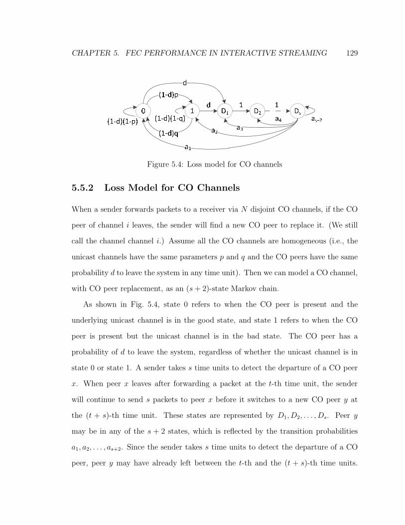
CHAPTER 5. FEC PERFORMANCE IN INTERACTIVE STREAMING 129
Figure 5.4: Loss model for CO channels
5.5.2 Loss Model for CO Channels
When a sender forwards packets to a receiver via N disjoint CO channels, if the CO
peer of channel i leaves, the sender will find a new CO peer to replace it. (We still
call the channel channel i.) Assume all the CO channels are homogeneous (i.e., the
unicast channels have the same parameters p and q and the CO peers have the same
probability d to leave the system in any time unit). Then we can model a CO channel,
with CO peer replacement, as an (s+ 2)-state Markov chain.
As shown in Fig. 5.4, state 0 refers to when the CO peer is present and the
underlying unicast channel is in the good state, and state 1 refers to when the CO
peer is present but the unicast channel is in the bad state. The CO peer has a
probability of d to leave the system, regardless of whether the unicast channel is in
state 0 or state 1. A sender takes s time units to detect the departure of a CO peer
x. When peer x leaves after forwarding a packet at the t-th time unit, the sender
will continue to send s packets to peer x before it switches to a new CO peer y at
the (t + s)-th time unit. These states are represented by D1, D2, . . . , Ds. Peer y
may be in any of the s + 2 states, which is reflected by the transition probabilities
a1, a2, . . . , as+2. Since the sender takes s time units to detect the departure of a CO
peer, peer y may have already left between the t-th and the (t + s)-th time units.

CHAPTER 5. FEC PERFORMANCE IN INTERACTIVE STREAMING 130
(The sender will know peer y has left and will not use peer y if it has left before the
t-th time unit). Peer y has an equal probability to have left in any of the s time
units, and the probability that peer y has left is 1− (1−d)s. Therefore, the transition
probabilities a3, a4, . . . , as+2 have a value of 1s(1 − (1 − d)s). By duality, we have
a1a2
= π1
π2= q
p. Now we can write the chain’s one-step probability transition matrix Pc
as
(1− p)(1− d) p(1− d) d 0 . . . 0
q(1− d) (1− q)(1− d) d 0 . . . 0
0 0 0 1 . . . 0
......
......
...
0 0 0 0 . . . 1
a1 a2 a3 a4 . . . as+2
where
a1 =q
p + q(1− d)s
a2 =p
p + q(1− d)s
ai =1− (1− d)s
s, 3 ≤ i ≤ s+ 2
(5.4)
The (s+ 2)-state Markov chain has stationary distribution π such that
πPc = π
s+2∑
i=1
πi = 1(5.5)
Solving the above equations, we have
π1 =q
p + q× (1− d)s
d× 1
α
π2 =p
p + q× (1− d)s
d× 1
α
πi+2 =i+ (s− i)(1− d)s
s× 1
α, 1 ≤ i ≤ s
(5.6)

CHAPTER 5. FEC PERFORMANCE IN INTERACTIVE STREAMING 131
where α = s+12
+ s−12
(1− d)s + 1d(1− d)s.
The CO channel’s packet loss ratio ec is the fraction of time that the chain stays in
states other than state 0, i.e., ec = 1−π1. The probability that a gap of length i occurs
between two bursts of non-zeros (i.e., states other than 0) is (1−d−p+pd)i(d+p−pd),
i.e., the gap length has a geometric distribution, and hence the average gap is 1d+p−dp
.
Since there are the same number of gaps and bursts, the average burst length is
lc = 1−ec
(d+p−dp)ec. However, the burst length no longer has a geometric distribution.
5.5.3 Post-FEC Loss Ratio
When N ≥ n disjoint channels exist with packet loss ratio ec, since each packet in
an FEC block is sent via a channel different from other packets in the FEC block,
whether the packet can reach the receiver without error is independent from the state
of other packets. Therefore, the probability P (m,n) that m packets are erroneous
out of n consecutive packets has a binomial distribution
P (m,n) =n!
m!(n−m)!emc (1− ec)n−m
Conditioning on the number of original packets lost in an FEC block, the post-FEC
loss ratio is
efec =1
k
k∑
i=1
iP (i, k)n−k∑
j=n−k+1−i
P (j, n− k) (5.7)
5.5.4 Numerical Results
Unless otherwise specified, we use the following default parameters. The streaming
rate is 480 Kbps for TV-quality video streaming, the packet size is 1500 bytes, and
thus 1 time unit is 25 milliseconds. We use an FEC block size of n = 16, which
CHAPTER 5. FEC PERFORMANCE IN INTERACTIVE STREAMING 132
introduces 400 milliseconds of coding delay. Internet link loss ratios vary greatly.
According to [50, 76], we use two loss ratios: 1% and 10%, and two burst lengths: 2
and 4. According to an empirical study [33], a peer’s average lifespan in a P2P system
is approximately 10 minutes; therefore the probability that a CO peer leaves in any
time unit is d = 140×60×10
. A sender takes 1 second to detect the departure of a CO
peer, i.e., s = 40. The numerical analysis program is written in the Java programming
language using the BigDecimal package for arbitrary-precision computing.6
Fig. 5.5 shows the post-FEC loss ratio when a sender uses N ≥ n disjoint CO
channels. First, in comparison to using the direct path, when multiple CO channels
are used, the post-FEC loss ratio decreases more sharply with the increasing number of
FEC packets, especially when Internet links have a lower loss ratio. This observation
indicates that path-diversity can improve FEC performance. Also note that the post-
FEC loss ratio is significantly lower when l is 2 than when l is 4 if the direct path is
used, but is not impacted by the burst length if N ≥ n CO channels is used.
Second, the use of CO peers achieves path diversity but also introduces extra
packet loss. This extra packet loss is more significant when Internet links have a low
packet loss ratio. (In Fig. 5.5, the post-FEC loss ratio when k is 16 equals the CO
channels’ loss ratio.) Compared with a unicast channel with parameters p and q,
an CO channel with parameters p, q, d and s has extra loss ratio ∆ = ec − e. From
6We have run simulations for all the numerical analysis. The simulation results are very closeto the numerical results. Except when the post-FEC packet loss ratio is less than 0.1%, the 95%confidence interval of the simulation result is within 5% of the corresponding numerical result.
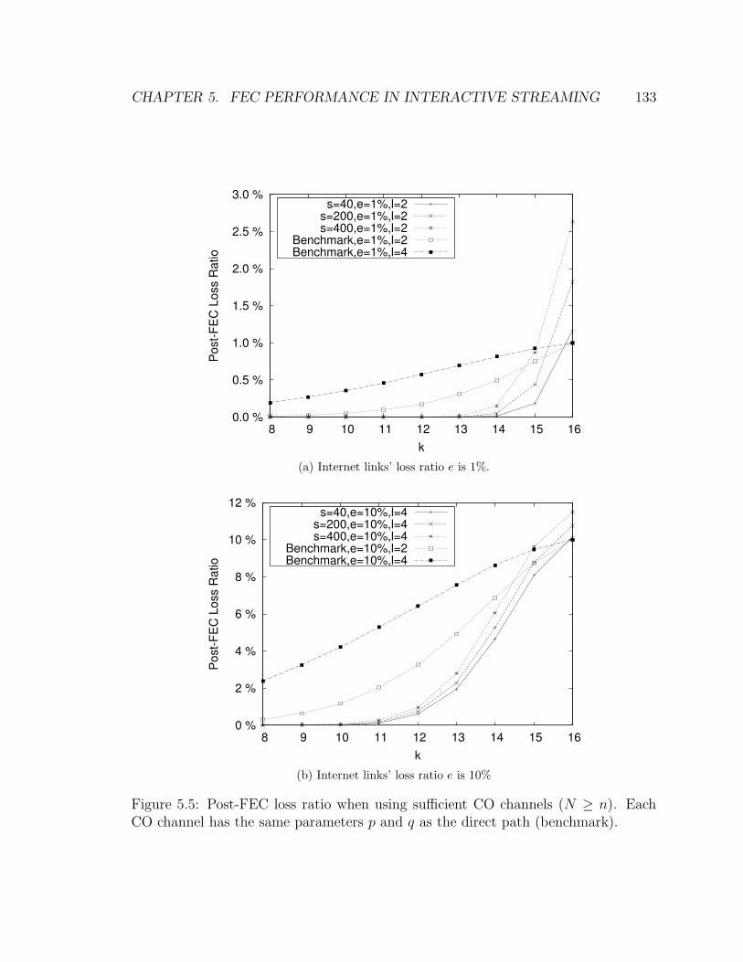
CHAPTER 5. FEC PERFORMANCE IN INTERACTIVE STREAMING 133
0.0 %
0.5 %
1.0 %
1.5 %
2.0 %
2.5 %
3.0 %
8 9 10 11 12 13 14 15 16
Po
st-
FE
C L
oss R
atio
k
s=40,e=1%,l=2s=200,e=1%,l=2s=400,e=1%,l=2
Benchmark,e=1%,l=2Benchmark,e=1%,l=4
(a) Internet links’ loss ratio e is 1%.
0 %
2 %
4 %
6 %
8 %
10 %
12 %
8 9 10 11 12 13 14 15 16
Po
st-
FE
C L
oss R
atio
k
s=40,e=10%,l=4s=200,e=10%,l=4s=400,e=10%,l=4
Benchmark,e=10%,l=2Benchmark,e=10%,l=4
(b) Internet links’ loss ratio e is 10%
Figure 5.5: Post-FEC loss ratio when using sufficient CO channels (N ≥ n). EachCO channel has the same parameters p and q as the direct path (benchmark).
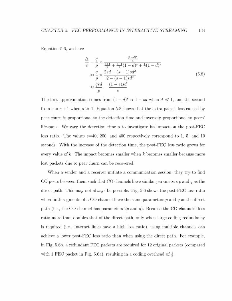
CHAPTER 5. FEC PERFORMANCE IN INTERACTIVE STREAMING 134
Equation 5.6, we have
∆
e=q
p×
(1−d)s
ds+12
+ s−12
(1− d)s + 1d(1− d)s
≈ q
p× 2sd− (s− 1)sd2
2− (s− 1)sd2
≈ qsd
p=
(1− e)sde
(5.8)
The first approximation comes from (1 − d)s ≈ 1 − sd when d ≪ 1, and the second
from s ≈ s+ 1 when s≫ 1. Equation 5.8 shows that the extra packet loss caused by
peer churn is proportional to the detection time and inversely proportional to peers’
lifespans. We vary the detection time s to investigate its impact on the post-FEC
loss ratio. The values s=40, 200, and 400 respectively correspond to 1, 5, and 10
seconds. With the increase of the detection time, the post-FEC loss ratio grows for
every value of k. The impact becomes smaller when k becomes smaller because more
lost packets due to peer churn can be recovered.
When a sender and a receiver initiate a communication session, they try to find
CO peers between them such that CO channels have similar parameters p and q as the
direct path. This may not always be possible. Fig. 5.6 shows the post-FEC loss ratio
when both segments of a CO channel have the same parameters p and q as the direct
path (i.e., the CO channel has parameters 2p and q). Because the CO channels’ loss
ratio more than doubles that of the direct path, only when large coding redundancy
is required (i.e., Internet links have a high loss ratio), using multiple channels can
achieve a lower post-FEC loss ratio than when using the direct path. For example,
in Fig. 5.6b, 4 redundant FEC packets are required for 12 original packets (compared
with 1 FEC packet in Fig. 5.6a), resulting in a coding overhead of 13.

CHAPTER 5. FEC PERFORMANCE IN INTERACTIVE STREAMING 135
0.0 %
0.4 %
0.8 %
1.2 %
1.6 %
2.0 %
2.4 %
2.8 %
3.2 %
3.6 %
4.0 %
8 9 10 11 12 13 14 15 16
Po
st-
FE
C L
oss R
atio
k
s=40s=200s=400
Benchmark
(a) Internet links’ loss ratio e is 1% and burst length l is 2.
0 %
4 %
8 %
12 %
16 %
20 %
8 9 10 11 12 13 14 15 16
Po
st-
FE
C L
oss R
atio
k
s=40s=200s=400
Benchmark
(b) Internet links’ loss ratio e is 10% and burst length l is 4.
Figure 5.6: Post-FEC loss ratio when using sufficient CO channels (N ≥ n). Eachof the two segments of a CO channel has the same parameters p and q as the directpath (benchmark).

CHAPTER 5. FEC PERFORMANCE IN INTERACTIVE STREAMING 136
5.6 FEC Performance With a Limited Number of
Disjoint CO Channels
When a sender sends packets via N disjoint CO channels in a round-robin fashion,
only 1N
of each channel is used. When N < n, the states of packets in an FEC block
are not independent. In this section, we first introduce the modeling of subchannels
of a CO channel, then compute the post-FEC loss ratio when N < n disjoint CO
channels exist between a sender and a receiver.
5.6.1 Subchannels of a CO Channel
We consider the two parts of a CO channel—the unicast channel and the CO peer—
separately. Given a unicast channel with one-step probability transition matrix P , its
subchannel can also be modeled as a 2-state Markov chain, and its one-step probability
transition matrix P ′ is the N -step probability matrix of the whole channel. By the
Chapman-Kolmogorov equations, P ′ = PN . It can be shown that
(
1−p pq 1−q
)N
=(1− p− q)N
p + q
(
p −p
−q q
)
+1
p+ q
(
q p
q p
)
From a subchannel’s perspective, if the CO peer is present for the current packet
at time t, it will leave with a probability of 1 − (1 − d)N before time t + N for the
next packet. When the CO peer leaves, the sender will continue to send ⌊ sN⌋ packets
to the CO peer. Therefore, the subchannel of a CO channel can be modeled as a

CHAPTER 5. FEC PERFORMANCE IN INTERACTIVE STREAMING 137
(⌊ sN⌋+ 2)-state Markov chain with parameters
p′ =p
p+ q(1− (1− p− q)N)
q′ =q
p+ q(1− (1− p− q)N)
d′ = 1− (1− d)N
s′ = ⌊ sN⌋
(5.9)
5.6.2 Post-FEC Loss Ratio
As in the case of using a single unicast channel to send packets, when the number
of channels N is less than the block size n, the state of a packet may depend on the
state of a previous packet in the same FEC block. To compute the post-FEC packet
loss ratio, we need to count the number of unrecoverable original packets lost in each
possible FEC block and compute its probability. We continue to use the algorithm
in Fig. 5. However, the generation of all the possible FEC blocks and computation
of their probabilities are different.
Assume N divides n and s. Let xi = (x1ix2i . . . xbi), where b = nN
, denote the sub-
sequence of channel i. Then an FEC block x consists of N interleaved subsequences,
x = (x11x12 . . . x1Nx21x22 . . . x2N . . . xb1xb2 . . . xbN)
Given the CO channel’s parameters p, q, d and s, the subchannel’s parameters
p′, q′, d′ and s′ can be computed by Equation 5.9. The subchannel’s transition matrix
P ′
c and stationary distribution π′ can be computed by Equation 5.4 and 5.6. Because
these N CO channels are disjoint, the probability of the FEC block x is the product of
the probabilities of subsequences, i.e., Pr{x} =∏Ni=1 Pr{xi}. The probability of each
sub-sequence can be computed using the algorithm in Fig. 6 (with the subchannel’s P ′

CHAPTER 5. FEC PERFORMANCE IN INTERACTIVE STREAMING 138
Algorithm 7 The algorithm to generate all the possible sequences of length b for aCO channel with detection time s′.
Input: seq and sequences are emptyOutput: sequences holds all the sequences of length b1: Procedure makeSequences()2: if seq.empty() or seq.top() = s′ + 1 then3: first← 0; last← s′ + 14: else if seq.top() ≤ 1 then5: first← 0; last← 26: else7: first← seq.top() + 1; last← first8: for first ≤ state ≤ last do9: seq.push(state)
10: if seq.size() = b then sequences.add(seq)11: else makeSequences()12: seq.pop(state)
and π′). The recursive algorithm to generate all the possible sequences of a subchannel
is shown in Fig. 7. The algorithm constructs a subsequence packet by packet. The
state of the first packet ranges from 0 to s′ + 1 (lines 2–3). If the state of the current
packet is 0 or 1, the next packet’s state ranges from 0 to 2 (lines 4–5). If the state of the
current packet is s′ +1, the next packet’s state ranges from 0 to s′ +1 (corresponding
to the situation that the sender replaces a departed CO peer with a new CO peer).
5.6.3 Numerical Results
Fig. 5.7 shows the post-FEC loss ratio when a sender usesN < n disjoint CO channels.
For every value of k, e and l, the post-FEC loss ratio drops when more channels are
used, but the decrease becomes marginal when N exceeds a certain value. As in the
case of using the direct path, a longer burst length results in a higher post-FEC loss
ratio. The increase is more significant when a sender uses fewer channels. This is
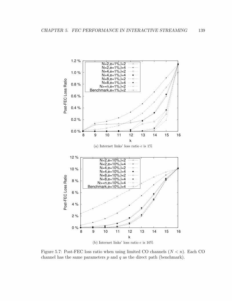
CHAPTER 5. FEC PERFORMANCE IN INTERACTIVE STREAMING 139
0.0 %
0.2 %
0.4 %
0.6 %
0.8 %
1.0 %
1.2 %
8 9 10 11 12 13 14 15 16
Po
st-
FE
C L
oss R
atio
k
N=2,e=1%,l=2N=2,e=1%,l=4N=4,e=1%,l=2N=4,e=1%,l=4N=8,e=1%,l=2N=8,e=1%,l=4
N>=n,e=1%,l=2Benchmark,e=1%,l=2
(a) Internet links’ loss ratio e is 1%
0 %
2 %
4 %
6 %
8 %
10 %
12 %
8 9 10 11 12 13 14 15 16
Po
st-
FE
C L
oss R
atio
k
N=2,e=10%,l=2N=2,e=10%,l=4N=4,e=10%,l=2N=4,e=10%,l=4N=8,e=10%,l=2N=8,e=10%,l=4
N>=n,e=10%,l=4Benchmark,e=10%,l=4
(b) Internet links’ loss ratio e is 10%
Figure 5.7: Post-FEC loss ratio when using limited CO channels (N < n). Each COchannel has the same parameters p and q as the direct path (benchmark).
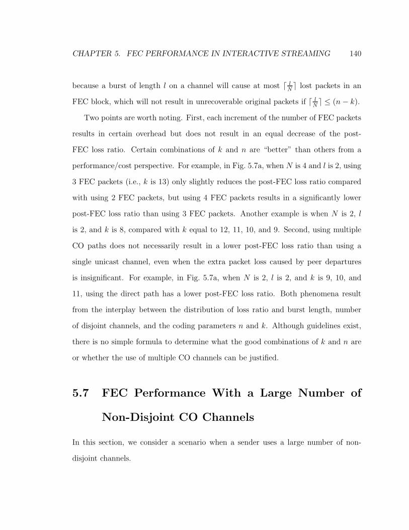
CHAPTER 5. FEC PERFORMANCE IN INTERACTIVE STREAMING 140
because a burst of length l on a channel will cause at most ⌈ lN⌉ lost packets in an
FEC block, which will not result in unrecoverable original packets if ⌈ lN⌉ ≤ (n− k).
Two points are worth noting. First, each increment of the number of FEC packets
results in certain overhead but does not result in an equal decrease of the post-
FEC loss ratio. Certain combinations of k and n are “better” than others from a
performance/cost perspective. For example, in Fig. 5.7a, when N is 4 and l is 2, using
3 FEC packets (i.e., k is 13) only slightly reduces the post-FEC loss ratio compared
with using 2 FEC packets, but using 4 FEC packets results in a significantly lower
post-FEC loss ratio than using 3 FEC packets. Another example is when N is 2, l
is 2, and k is 8, compared with k equal to 12, 11, 10, and 9. Second, using multiple
CO paths does not necessarily result in a lower post-FEC loss ratio than using a
single unicast channel, even when the extra packet loss caused by peer departures
is insignificant. For example, in Fig. 5.7a, when N is 2, l is 2, and k is 9, 10, and
11, using the direct path has a lower post-FEC loss ratio. Both phenomena result
from the interplay between the distribution of loss ratio and burst length, number
of disjoint channels, and the coding parameters n and k. Although guidelines exist,
there is no simple formula to determine what the good combinations of k and n are
or whether the use of multiple CO channels can be justified.
5.7 FEC Performance With a Large Number of
Non-Disjoint CO Channels
In this section, we consider a scenario when a sender uses a large number of non-
disjoint channels.

CHAPTER 5. FEC PERFORMANCE IN INTERACTIVE STREAMING 141
Figure 5.8: Abstract topology when a sender uses a large number of non-disjointpaths to send packets to a receiver. Dashed lines are error-free virtual links.
5.7.1 Loss Model For Non-Disjoint CO Channels
As discussed in Section 5.3.2, the paths between a sender and a receiver are two
SPTs on the substrate Internet, rooted at the sender and receiver respectively with
CO peers as leaves. The number of unique IP addresses is small close to the tree root
but becomes sufficiently large (compared to the FEC block size n) beyond certain
points. These turning points are usually the PoPs but may be a few hops beyond the
PoPs. For convenience, we still use the term PoPs to refer to these turning points.
We call the segments before PoPs the access segments and beyond PoPs the core
segments. The large number of non-disjoint CO channels can be deemed as consisting
of three sections: two access sections and a core section. In an access section, a
sender (or receiver) connects to N PoPs. In the core section, there exist enough
disjoint paths between PoPs. When a sender and a receiver initiate a communication
session or select a CO peer to replace a departed CO peer, they select CO peers
such that packets in an FEC block are spread evenly across the N access segments to
achieve the maximum possible path diversity. (These CO peers can be found by using
virtual network position schemes and position-based routing schemes mentioned in

CHAPTER 5. FEC PERFORMANCE IN INTERACTIVE STREAMING 142
Section 5.3.1.) Assume the N access segments from a sender (or receiver) to its PoPs
are disjoint and there are the same number of access segments at the sender side and
the receiver side7. Because the state of each segment and CO peer is independent
from the others, we can move the access segments at the sender side and receiver side
together, and move the CO peer right before the receiver. Fig. 5.8 shows the resulting
abstract topology. There are N < n disjoint unicast channels from the sender to N
PoPs and sufficient CO channels from each PoP to the receiver.
Assume the access segments account for a fraction β of the packet loss of the whole
unicast channel (not including the packet loss caused by peer departures). Then each
of the N unicast channels between the sender and the PoPs can be modeled using a
2-state Markov chain with parameters βp and q. A packet that fails to reach a PoP
will not reach the receiver, and a packet that reaches a PoP will reach the receiver
with a probability of θ. Since sufficient disjoint paths exist between a PoP and the
receiver, and no two packets in an FEC block are transmitted via the same channel,
whether or not the packet can reach the receiver from a PoP is independent from the
states of other packets in the FEC block. The probability θ is the loss ratio of the
CO channel from a PoP to the receiver (consisting of the core segment and the CO
peer), which can be computed by Equation 5.7 with parameters (1 − β)p, q, d and s
using the method introduced in Sections 5.5.2 and 5.5.3. Therefore, the large number
of non-disjoint CO channels between a sender and a receiver can be considered as
N < n disjoint channels where each channel follows a variant Gilbert model. The
variant Gilbert model has two states and parameters βp and q. Packets will be lost if
7If the N access segments are not disjoint or there are different numbers of access segments at thesender side and the receiver side, we can further divide the two access sections into a series of smallsections such that links in each section are disjoint. The post-FEC loss ratio can still be computedby counting the number of unrecoverable packets lost in each possible FEC block and computing itsprobability, but the algorithm will have a larger complexity.

CHAPTER 5. FEC PERFORMANCE IN INTERACTIVE STREAMING 143
the channel is in the bad state and will have a probability of θ to be erroneous when
the channel is in the good state.
5.7.2 Post-FEC Loss Ratio
Let 0g denote that the channel is in the good state and the packet is error-free, let
0e denote that the channel is in the good state but the packet is erroneous, and let 1
denote that the channel is in the bad state. As in the case of using the direct path
and a limited number of disjoint CO channels, to compute the post-FEC loss ratio,
we need to count the number of unrecoverable packets lost in each possible FEC
block and compute its probability, i.e., we continue to use the algorithm in Fig. 5.
Assume N divides n and s. Let xi = (x1ix2i . . . xbi), where b = nN
and xji ∈ {0g, 0e, 1},
denote the subsequence of channel i. Then an FEC block x consists of N interleaved
subsequences. It is easy to count the number of unrecoverable original packets. The
probability of an FEC block is the product of the probabilities of all the subsequences.
The probability of each subsequence is computed by converting the variant Gilbert
model to a 3-state Markov chain with one-step probability matrix P ′
(1− βp)(1− θ) (1− βp)θ βp
(1− βp)(1− θ) (1− βp)θ βp
q(1− θ) qθ (1− q)
The stationary distribution π′ of the 3-state Markov chain can be obtained easily.
The probability of each subsequence can be computed using the algorithm shown in
Fig. 6 (with P ′ and π′).

CHAPTER 5. FEC PERFORMANCE IN INTERACTIVE STREAMING 144
0.0 %
0.2 %
0.4 %
0.6 %
0.8 %
1.0 %
1.2 %
8 9 10 11 12 13 14 15 16
Po
st-
FE
C L
oss R
atio
k
β=0.25β=0.5
β=0.75β=0
2 PathsBenchmark
(a) Internet links’ loss ratio e is 1% and burst length l is 2.
0 %
2 %
4 %
6 %
8 %
10 %
12 %
8 9 10 11 12 13 14 15 16
Po
st-
FE
C L
oss R
atio
k
β=0.25β=0.5
β=0.75β=0
2 PathsBenchmark
(b) Internet links’ loss ratio e is 10% and burst length l is 4.
Figure 5.9: Post-FEC loss ratio when using a large number of non-disjoint CO chan-nels. Each CO channel has the same parameters p and q as the direct path (bench-mark). The access segment has 2 disjoint paths.
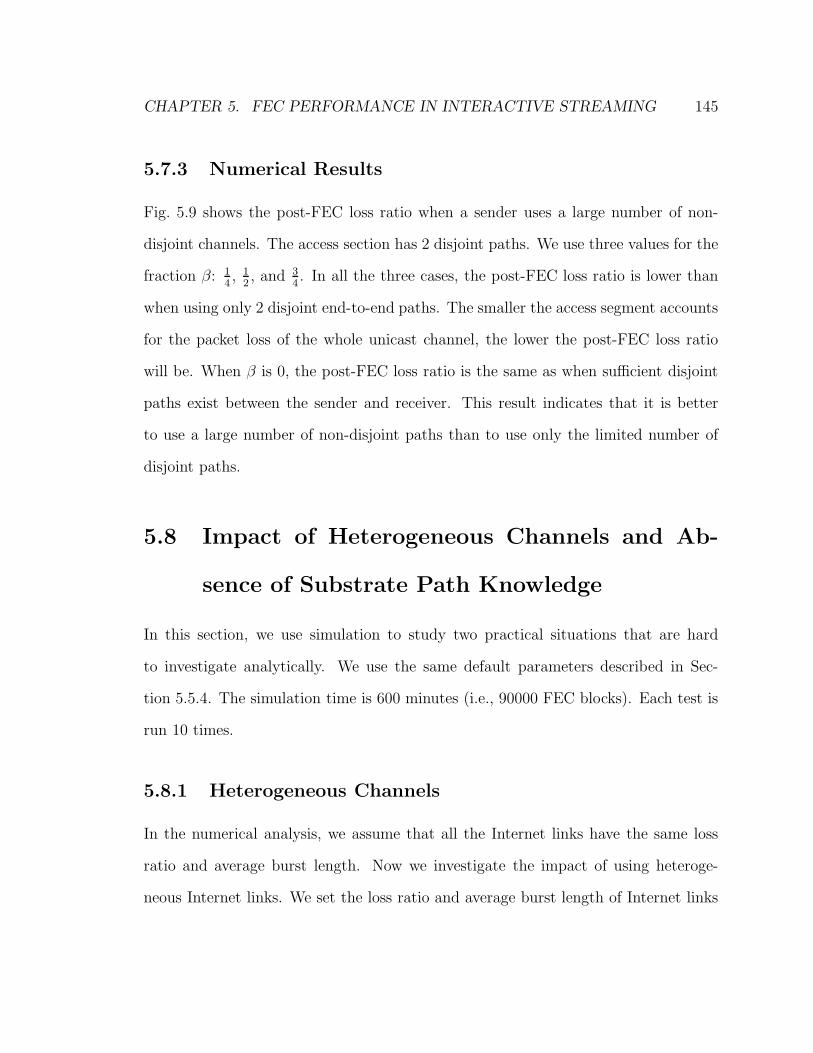
CHAPTER 5. FEC PERFORMANCE IN INTERACTIVE STREAMING 145
5.7.3 Numerical Results
Fig. 5.9 shows the post-FEC loss ratio when a sender uses a large number of non-
disjoint channels. The access section has 2 disjoint paths. We use three values for the
fraction β: 14, 1
2, and 3
4. In all the three cases, the post-FEC loss ratio is lower than
when using only 2 disjoint end-to-end paths. The smaller the access segment accounts
for the packet loss of the whole unicast channel, the lower the post-FEC loss ratio
will be. When β is 0, the post-FEC loss ratio is the same as when sufficient disjoint
paths exist between the sender and receiver. This result indicates that it is better
to use a large number of non-disjoint paths than to use only the limited number of
disjoint paths.
5.8 Impact of Heterogeneous Channels and Ab-
sence of Substrate Path Knowledge
In this section, we use simulation to study two practical situations that are hard
to investigate analytically. We use the same default parameters described in Sec-
tion 5.5.4. The simulation time is 600 minutes (i.e., 90000 FEC blocks). Each test is
run 10 times.
5.8.1 Heterogeneous Channels
In the numerical analysis, we assume that all the Internet links have the same loss
ratio and average burst length. Now we investigate the impact of using heteroge-
neous Internet links. We set the loss ratio and average burst length of Internet links

CHAPTER 5. FEC PERFORMANCE IN INTERACTIVE STREAMING 146
0.0 %
0.2 %
0.4 %
0.6 %
0.8 %
1.0 %
1.2 %
8 9 10 11 12 13 14 15 16
Po
st-
FE
C L
oss R
atio
k
Heterogeneous, N=2Homogeneous, N=2
Heterogeneous, N>=nHomogeneous, N>=n
(a) e is U(0, 2%) and l is U(1, 3).
0 %
2 %
4 %
6 %
8 %
10 %
12 %
8 9 10 11 12 13 14 15 16
Po
st-
FE
C L
oss R
atio
k
Heterogeneous, N=2Homogeneous, N=2
Heterogeneous, N>=nHomogeneous, N>=n
(b) e is U(0, 20%) and l is U(1, 7).
Figure 5.10: Post-FEC loss ratio when using heterogeneous CO channels. Internetlinks’ loss ratio e and burst length l are uniformly distributed.

CHAPTER 5. FEC PERFORMANCE IN INTERACTIVE STREAMING 147
0
0.2
0.4
0.6
0.8
1
1.2
1.4
0.0 % 0.5 % 1.0 % 1.5 % 2.0 % 2.5 %
Pro
ba
bili
ty D
en
sity
HomogeneousHeteromogeneous
Figure 5.11: Comparison of the probability density of the post-FEC loss ratio whenInternet links are homogeneous (e is 1% and l is 2) and heterogeneous (e is U(0, 2%)and l is U(1, 3). The sender uses N=2 disjoint paths and k=15.
according to a uniform distribution with the means equal to that of the homoge-
neous case. Fig. 5.10 compares the post-FEC loss ratio when using heterogeneous
and homogeneous Internet links. When a sender uses N ≥ n disjoint CO channels,
there is no discernible difference. When a sender uses N=2 disjoint CO channels, the
heterogeneous case has a slightly lower post-FEC loss ratio.
In the heterogeneous case, because of peer churn, the set of channels a sender
uses has different loss ratios and burst lengths at different times, so we continue to
investigate the post-FEC loss ratio from a temporal perspective. To examine whether
the post-FEC loss ratio fluctuates more severely in the heterogeneous case than in
the homogeneous case, we first calculate the post-FEC loss ratio per minute, and
then obtain the probability density function (PDF) using kernel density estimation
(Gaussian kernel with bandwidth of 0.1). Fig. 5.11 shows a sample comparison of the
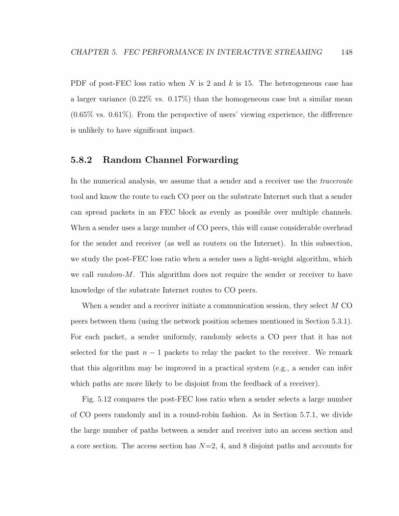
CHAPTER 5. FEC PERFORMANCE IN INTERACTIVE STREAMING 148
PDF of post-FEC loss ratio when N is 2 and k is 15. The heterogeneous case has
a larger variance (0.22% vs. 0.17%) than the homogeneous case but a similar mean
(0.65% vs. 0.61%). From the perspective of users’ viewing experience, the difference
is unlikely to have significant impact.
5.8.2 Random Channel Forwarding
In the numerical analysis, we assume that a sender and a receiver use the traceroute
tool and know the route to each CO peer on the substrate Internet such that a sender
can spread packets in an FEC block as evenly as possible over multiple channels.
When a sender uses a large number of CO peers, this will cause considerable overhead
for the sender and receiver (as well as routers on the Internet). In this subsection,
we study the post-FEC loss ratio when a sender uses a light-weight algorithm, which
we call random-M . This algorithm does not require the sender or receiver to have
knowledge of the substrate Internet routes to CO peers.
When a sender and a receiver initiate a communication session, they select M CO
peers between them (using the network position schemes mentioned in Section 5.3.1).
For each packet, a sender uniformly, randomly selects a CO peer that it has not
selected for the past n − 1 packets to relay the packet to the receiver. We remark
that this algorithm may be improved in a practical system (e.g., a sender can infer
which paths are more likely to be disjoint from the feedback of a receiver).
Fig. 5.12 compares the post-FEC loss ratio when a sender selects a large number
of CO peers randomly and in a round-robin fashion. As in Section 5.7.1, we divide
the large number of paths between a sender and receiver into an access section and
a core section. The access section has N=2, 4, and 8 disjoint paths and accounts for

CHAPTER 5. FEC PERFORMANCE IN INTERACTIVE STREAMING 149
0.0 %
0.2 %
0.4 %
0.6 %
0.8 %
1.0 %
1.2 %
8 9 10 11 12 13 14 15 16
Po
st-
FE
C L
oss R
atio
k
N=2, randomN=4, randomN=8, random
N=2, round-robinN=4, round-robinN=8, round-robin
(a) Internet links’ loss ratio e is 1% and burst length l is 2.
0 %
2 %
4 %
6 %
8 %
10 %
12 %
8 9 10 11 12 13 14 15 16
Po
st-
FE
C L
oss R
atio
k
N=2, randomN=4, randomN=8, random
N=2, round-robinN=4, round-robinN=8, round-robin
(b) Internet links’ loss ratio e is 10% and burst length l is 4.
Figure 5.12: Post-FEC loss ratio when using a large number of random CO peers.The fraction of access segments account for β = 0.25 of total packet loss.
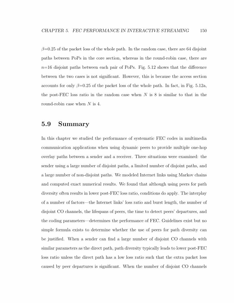
CHAPTER 5. FEC PERFORMANCE IN INTERACTIVE STREAMING 150
β=0.25 of the packet loss of the whole path. In the random case, there are 64 disjoint
paths between PoPs in the core section, whereas in the round-robin case, there are
n=16 disjoint paths between each pair of PoPs. Fig. 5.12 shows that the difference
between the two cases is not significant. However, this is because the access section
accounts for only β=0.25 of the packet loss of the whole path. In fact, in Fig. 5.12a,
the post-FEC loss ratio in the random case when N is 8 is similar to that in the
round-robin case when N is 4.
5.9 Summary
In this chapter we studied the performance of systematic FEC codes in multimedia
communication applications when using dynamic peers to provide multiple one-hop
overlay paths between a sender and a receiver. Three situations were examined: the
sender using a large number of disjoint paths, a limited number of disjoint paths, and
a large number of non-disjoint paths. We modeled Internet links using Markov chains
and computed exact numerical results. We found that although using peers for path
diversity often results in lower post-FEC loss ratio, conditions do apply. The interplay
of a number of factors—the Internet links’ loss ratio and burst length, the number of
disjoint CO channels, the lifespans of peers, the time to detect peers’ departures, and
the coding parameters—determines the performance of FEC. Guidelines exist but no
simple formula exists to determine whether the use of peers for path diversity can
be justified. When a sender can find a large number of disjoint CO channels with
similar parameters as the direct path, path diversity typically leads to lower post-FEC
loss ratio unless the direct path has a low loss ratio such that the extra packet loss
caused by peer departures is significant. When the number of disjoint CO channels
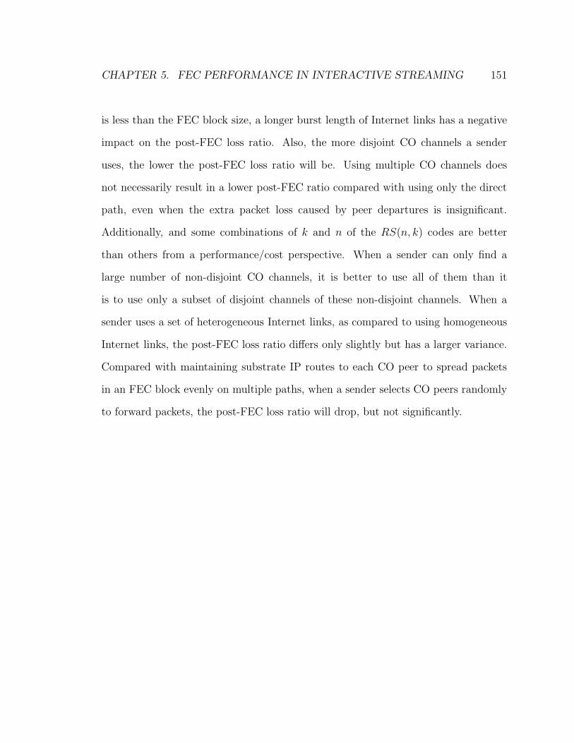
CHAPTER 5. FEC PERFORMANCE IN INTERACTIVE STREAMING 151
is less than the FEC block size, a longer burst length of Internet links has a negative
impact on the post-FEC loss ratio. Also, the more disjoint CO channels a sender
uses, the lower the post-FEC loss ratio will be. Using multiple CO channels does
not necessarily result in a lower post-FEC ratio compared with using only the direct
path, even when the extra packet loss caused by peer departures is insignificant.
Additionally, and some combinations of k and n of the RS(n, k) codes are better
than others from a performance/cost perspective. When a sender can only find a
large number of non-disjoint CO channels, it is better to use all of them than it
is to use only a subset of disjoint channels of these non-disjoint channels. When a
sender uses a set of heterogeneous Internet links, as compared to using homogeneous
Internet links, the post-FEC loss ratio differs only slightly but has a larger variance.
Compared with maintaining substrate IP routes to each CO peer to spread packets
in an FEC block evenly on multiple paths, when a sender selects CO peers randomly
to forward packets, the post-FEC loss ratio will drop, but not significantly.
Chapter 6
Conclusions and Future Directions
6.1 Conclusions
Video streaming applications have become wildly popular on the Internet. According
to the playback delay, video streaming can be classified into on-demand streaming,
live streaming, and interactive streaming. Live streaming applications may have
an arbitrary number of receivers, while interactive streaming applications typically
have a small group size. To reduce financial expenditure and improve scalability, live
streaming applications often adopt the P2P model to utilize users’ upload bandwidth.
Interactive streaming applications usually use the C/S model but may use peers to
achieve path diversity or traverse firewall and NAT devices.
For P2P video streaming applications, smoothness and timeliness of the playback
are the two most important aspects of users’ viewing experiences, whereas the amount
of Internet traffic is the main concern of ISPs. The goal of this thesis was to study
traffic locality and reliable delivery of packets in large-scale live streaming and small-
scale interactive streaming applications, while keeping the playback delay well below
152

CHAPTER 6. CONCLUSIONS AND FUTURE DIRECTIONS 153
the limit that the targeted application can tolerate. More specifically, we addressed
two problems.
The first problem we addressed is how to localize video traffic without jeopardiz-
ing users’ viewing experiences in large-scale P2P live streaming applications. Real-
world P2P live streaming deployments use the swarm-based or data-driven tree-based
schemes. Therefore, we first investigated whether the neighbor-with-nearby-peers
strategy, which was originally proposed for P2P file sharing applications, is applica-
ble to P2P live streaming applications. We identified a “typical” swarm-based scheme
and a data-driven tree-based scheme that capture the essential aspects of these two
types of schemes. We compare system performance of the two typical schemes on two
types of neighboring overlays: random overlay where peers select neighbors randomly,
and nearby overlay where peers use the neighbor-with-nearby-peers strategy and only
select nearby peers as neighbors. We developed a discrete-event simulator to study
system performance of the two typical schemes on the two overlays, and proposed
packet propagation models to analyze the paths packets propagate on a given overlay
and overlay models to characterize the random and nearby overlays and analyze their
impact on system performance.
We found that packets propagate in distinct manners in the swarm-based scheme
and tree-based scheme although both schemes are data-driven. In the swarm-based
scheme, peers have a high probability to pull from neighbors that have fewer hops to
the source peer; the set of paths a chunk traverses from the source to peers is close to
a degree-bounded shortest path tree (in term of hops) on the neighboring overlay. In
the tree-based scheme, because of the short-circuit effect, peers select parents almost
randomly with respect to their hop counts to the source, resulting in significantly
CHAPTER 6. CONCLUSIONS AND FUTURE DIRECTIONS 154
taller propagation trees compared to the swarm-based scheme. The neighbor-with-
nearby-peers strategy reduces network traffic significantly, but also results in more
lost packets in the presence of peer churn and substrate network errors because of the
large diameter and clustering coefficient of the nearby overlay. The different chunk
propagation behaviors of the swarm-based and tree-based schemes cause chunk loss in
different ways in the two schemes. The neighbor-with-nearby-peers strategy causes
more chunk loss in the tree-based schemes than in the swarm-based schemes. On
one hand, our work explains why commercial deployments, which construct random
overlays and use the data-driven approach, usually have good performance. Our work
also shows that simply applying the neighbor-with-nearby-peers strategy deteriorates
the quality of their services. On the other hand, our work furthers the understanding
of data-driven video live streaming schemes and suggests that new schemes should use
the network-driven approach to control chunks’ propagation paths to localize video
traffic while maintaining service quality.
In light of the above findings, we propose a neighboring strategy to construct a
hierarchical overlay and a network-driven tree-building algorithm. Our idea is to first
identify the desired shape of propagation trees, then construct the neighboring overlay
to be the super graph of these trees, and use the tree-building algorithm to construct
trees with the desired shape on the neighboring overlay. On the hierarchical overlay,
most edges are between nearby peers to reduce network traffic, but a small fraction
of edges are rewired to remote peers in a way that the neighboring overlay exhibits a
hierarchical structure. The tree-building algorithm, called TreeClimber, is a DV-style
routing protocol that heuristically constructs a DBMST, with respect to hops, on
a neighboring overlay. The swarm technique is used for multi-point re-transmission

CHAPTER 6. CONCLUSIONS AND FUTURE DIRECTIONS 155
error-correction mechanism and has no impact on the shape of propagation trees.
We compared our network-driven tree-building scheme with the typical data-driven
tree-based scheme and compared the hierarchical overlay with the random overlay
and small-world overlay. Simulation results show that our scheme outperforms the
typical data-driven tree-based scheme and that the hierarchical overlay outperforms
the small-world overlay. More users receive all the video chunks in TreeClimber than
in the typical data-driven tree-based scheme. The network cost of the hierarchical
overlay is only 13
of that on the random overlay, and the chunk delivery rate is close
to that on the random overlay under loose upload bandwidth constraints.
The second problem we addressed is the efficacy of systematic FEC for reducing
the packet loss rate perceived by the receiver without causing significant playback
delay and overhead in small-scale interactive streaming applications. FEC is the
preferred error correction technique for interactive streaming applications. Since it is
vulnerable to bursty packet loss of Internet links, P2P networks are used to provide
multiple one-hop overlay paths between two communication parties. We studied FEC
performance in three situations of path diversity—a sender using a large number of
disjoint paths, a limited number of disjoint paths, and a large number of non-disjoint
paths. We modeled Internet links using discrete-time Markov chains and provided
numerical analysis of the post-FEC loss ratio. We also used simulation to investigate
FEC performance in situations where the multiple paths are heterogeneous or a sender
lacks the knowledge of which paths are disjoint.
We found that although using peers for path diversity often results in a lower post-
FEC packet loss ratio, conditions do apply. The interplay of a number of factors—
the Internet links’ loss ratio and burst length, the number of disjoint CO channels,
CHAPTER 6. CONCLUSIONS AND FUTURE DIRECTIONS 156
the lifespans of peers, the time required to detect peers’ departures, and the coding
parameters—determines the performance of FEC. Guidelines exist, but some con-
ditions do apply. When a sender can find a large number of disjoint CO channels
with parameters similar to the direct path, path diversity typically leads to a lower
post-FEC loss ratio unless the direct path has a low loss ratio such that the extra
packet loss caused by peer departures is significant. When the number of disjoint CO
channels is less than the FEC block size, a longer burst length of Internet links has
a negative impact on the post-FEC loss ratio, and the more disjoint CO channels a
sender uses, the lower the post-FEC loss ratio will be. Using multiple CO channels
does not necessarily result in a lower post-FEC ratio as compared to with using only
the direct path, even when the extra packet loss caused by peer departures is insignif-
icant, and some combinations of k and n of the RS(n, k) codes are better than others
from a performance/cost perspective. When a sender can only find a large number
of non-disjoint CO channels, it is better to use all of them than it is to use only a
subset of disjoint channels of these non-disjoint channels. When a sender uses a set
of heterogeneous Internet links, in contrast to using homogeneous Internet links, the
post-FEC loss ratio differs only slightly but has a larger variance. In comparison
to maintaining substrate IP routes to each CO peer to spread packets in an FEC
block evenly on multiple paths, when a sender selects CO peers randomly to forward
packets, the post-FEC loss ratio will drop, but not significantly.
6.2 Future Directions
Video streaming traffic will undoubtedly continue to be the dominant type of traffic
on the Internet in the foreseeable future and both the C/S and P2P models will play
CHAPTER 6. CONCLUSIONS AND FUTURE DIRECTIONS 157
an important role in delivering video content. For large-scale P2P live streaming
applications, when a sufficient playback delay is allowed, the swarm technique can
guarantee a packet delivery rate of 100% because lost packets can be requested and
re-transmitted. However, in swarm-based schemes, each hop takes a long time and
the playback delay can easily exceed several minutes. Building a tree to push pack-
ets can greatly reduce the required playback delay. In tree-based schemes with the
swarm technique as a multi-point re-transmission mechanism, packets are pushed in
most hops and pulled in only a couple of hops, and thus a much shorter playback
delay can be used. Given a playback delay, which should be longer than the average
packet delivery delay plus several times of its standard deviation, the packet delivery
rate is determined by the deviation of the packet delivery delay. Packets follow dif-
ferent paths from the video source to a peer due to peer churn. It is preferable that
these paths have fewer overlaps, but similar numbers of hops. The network-driven
approach is superior to the data-driven approach because the latter lacks the ability
to control the propagation paths of packets. Therefore, network-driven tree-based
schemes with the swarm technique as a multi-point re-transmission mechanism pro-
vide a promising direction for P2P live streaming applications. In this thesis we have
considered the propagation tree shape, peers positions on the substrate Internet, and
peers’ upload capacities in the tree-building algorithm. System performance can be
further improved by considering a number of other factors, such as the bandwidth
and error rates of links to neighbors, the lifetime and activity history of neighbors.
For example, a peer can monitor the bandwidths and error rates metrics of links to
neighbors and replace neighbors with less bandwidths and higher error rates with
better neighbors. Another method to improve system performances is to introduce a

CHAPTER 6. CONCLUSIONS AND FUTURE DIRECTIONS 158
small number of dedicated servers into a P2P network. These servers can act as the
proxy video sources or as the last resort for peers to re-transmit lost packets.
Interactive streaming applications rely on coding schemes and path diversity for
protection against failures and bursty errors of Internet links. The packet loss rate
after error-correction can be improved along three directions. The first direction is
multi-layer source coding. Continuous research efforts have been and will be put into
developing highly-efficient multi-layer video coding schemes. The second direction
is to improve the quality of paths, and in case these paths have different quality, to
exploit the difference of quality for unequal path protection. A P2P network may have
a reputation system such that a sender and a receiver can select peers less likely to
leave abruptly as intermediate helper nodes. A sender can transmit critical packets,
such as I-frame packets or the original packets of an FEC block, via more reliable
paths and transmit less critical packets via less reliable paths. The third direction is
to use rateless channel coding schemes when the RTT between a sender and a receiver
is small. With a small RTT, the communication overhead is acceptable.

Bibliography
[1] V. Aggarwal, A. Feldmann, and C. Scheideler. Can ISPS and P2P users coop-
erate for improved performance? ACM SIGCOMM Computer Communication
Review, 37(3):40, 2007.
[2] S. Ali, A. Mathur, and H. Zhang. Measurement of commercial peer-to-peer
live video streaming. In Proc. of Workshop in Recent Advances in Peer-to-Peer
Streaming, pages 1–12, 2006.
[3] S. Androutsellis-Theotokis and D. Spinellis. A survey of peer-to-peer content
distribution technologies. ACM Computing Surveys, 36(4):335–371, 2004.
[4] S. Banerjee, B. Bhattacharjee, and C. Kommareddy. Scalable application layer
multicast. In Proc. ACM SIGCOMM Conf. on Applications, Technologies, Ar-
chitectures, and Protocols for Computer Communication, volume 32, pages 205–
217, 2002.
[5] S. Banerjee, C. Kommareddy, K. Kar, B. Bhattacharjee, and S. Khuller. Con-
struction of an efficient overlay multicast infrastructure for real-time applica-
tions. In Proc. IEEE INFOCOM, volume 2, pages 1521–1531, 2003.
159

BIBLIOGRAPHY 160
[6] A.C. Begen, Y. Altunbasak, and O. Ergun. Multi-path selection for multiple
description encoded video streaming. In IEEE Int. Conf. on Communications
(ICC), volume 3, pages 1583–1589, 2003.
[7] T. Bonald, L. Massoulie, F. Mathieu, D. Perino, and A. Twigg. Epidemic
live streaming: optimal performance trade-offs. In Proc. ACM SIGMETRICS
Int. Conf. on Measurement and Modeling of Computer Systems, pages 325–336,
2008.
[8] M. Castro, P. Druschel, A. M. Kermarrec, A. Nandi, A. Rowstron, and A. Singh.
Splitstream: High-bandwidth multicast in cooperative environments. ACM
SIGOPS Operating Systems Review, 37(5):298–313, 2003.
[9] K.-H.K. Chan, S.-H.G. Chan, and A.C. Begen. Spanc: Optimizing scheduling
delay for peer-to-peer live streaming. IEEE Trans. on Multimedia, 12(7):743–
753, 2010.
[10] Yatin Chawathe. Scattercast: an adaptable broadcast distribution framework.
Multimedia Systems, 9(1):104–118, 2003.
[11] D.R. Choffnes and F.E. Bustamante. Taming the Torrent: a practical approach
to reducing cross-ISP traffic in peer-to-peer systems. ACM SIGCOMM Com-
puter Communication Review, 38(4):363–374, 2008.
[12] Y. Chu, SG Rao, S. Seshan, and H. Zhang. A case for end system multicast.
IEEE Journal on Selected Areas in Communications, 20(8):1456–1471, 2002.
BIBLIOGRAPHY 161
[13] D. Ciullo, M.A. Garcia, A. Horvath, E. Leonardi, M. Mellia, D. Rossi, M. Telek,
and P. Veglia. Network awareness of p2p live streaming applications: A mea-
surement study. IEEE Trans. on Multimedia, 12(1):54–63, 2010.
[14] B. Cohen. Incentives build robustness in BitTorrent. In Workshop on Economics
of Peer-to-Peer Systems, volume 6, pages 68–72, 2003.
[15] F. Dabek, R. Cox, F. Kaashoek, and R. Morris. Vivaldi: A decentralized net-
work coordinate system. ACM SIGCOMM Computer Communication Review,
34(4):15–26, 2004.
[16] S.E. Deering and D.R. Cheriton. Multicast routing in datagram internetworks
and extended LANs. ACM Trans. on Computer Systems, 8(2):85–110, 1990.
[17] E.O Elliot. A model of the switched telephone network for data communications.
Bell System Technical Journal, 44(1):89, 1965.
[18] S. Fashandi, S.O. Gharan, and A.K. Khandani. Path diversity over packet
switched networks: Performance analysis and rate allocation. IEEE/ACM
Trans. on Networking, 18(5):1373–1386, 2010.
[19] F.H.P. Fitzek, B. Can, R. Prasad, and M. Katz. Overhead and quality mea-
surements for multiple description coding for video services. Wireless Personal
Multimedia Communications, 2:524–528, 2004.
[20] P. Francis. Yoid: Extending the Internet multicast architecture. 2000.
[21] P. Frossard. FEC performance in multimedia streaming. IEEE Communications
Letters, 5(3):122–124, 2001.
BIBLIOGRAPHY 162
[22] AJ Ganesh, A. M. Kermarrec, and L. MassoulieCa. Peer-to-peer membership
management for gossip-based protocols. IEEE Trans. on Computers, 52(2):139–
149, 2003.
[23] E.N. Gilbert. Capacity of a burst-noise channel. Bell System Technical Journal,
39(9):1253–1265, 1960.
[24] S. Giordano, I. Stojmenovic, and L. Blazevic. Position based routing algorithms
for ad hoc networks: a taxonomy. Ad Hoc Wireless Networking, pages 103–136,
2004.
[25] V.K Goyal. Multiple description coding: Compression meets the network. IEEE
Signal Processing Magazine, 18(5):74–93, 2001.
[26] K.P. Gummadi, H.V. Madhyastha, S.D. Gribble, H.M. Levy, and D. Wetherall.
Improving the reliability of Internet paths with one-hop source routing. In Proc.
Conf. on Symp. on Opearting Systems Design and Implementation, volume 6,
pages 13–13, 2004.
[27] M. Hefeeda and H. Saleh. Traffic modeling and proportional partial caching
for peer-to-peer systems. IEEE/ACM Trans. on Networking, 16(6):1447–1460,
2008.
[28] J. Jannotti, D. K. Gifford, K. L. Johnson, M. F. Kaashoek, and J. W. O’Toole
Jr. Overcast: reliable multicasting with on overlay network. In Proc. Symp. on
Operating System Design and Implementation (OSDI), pages 14–30, 2000.

BIBLIOGRAPHY 163
[29] X. Jin, K.L. Cheng, and S.H.G. Chan. Island multicast: Combining IP multicast
with overlay data distribution. IEEE Trans. on Multimedia, 11(5):1024–1036,
2009.
[30] M. Kobayashi, H. Nakayama, N. Ansari, and N. Kato. Robust and efficient
stream delivery for application layer multicasting in heterogeneous networks.
IEEE Trans. on Multimedia, 11(1):166–176, 2009.
[31] B. Krishnamurthy and J. Wang. On network-aware clustering of web clients.
In Proc. ACM SIGCOMM Conf. on Applications, Technologies, Architectures,
and Protocols for Computer Communication, pages 97–110, 2000.
[32] J. Kubiatowicz, D. Bindel, Y. Chen, S. Czerwinski, P. Eaton, D. Geels, R. Gum-
madi, S. Rhea, H. Weatherspoon, and C. Wells. Oceanstore: An architecture for
global-scale persistent storage. ACM SIGARCH Computer Architecture News,
28(5):190–201, 2000.
[33] B. Li, S. Xie, G. Y. Keung, J. Liu, I. Stoica, H. Zhang, and X. Zhang. An
empirical study of the Coolstreaming system. IEEE Journal on Selected Areas
in Communications, 25(9):1627–1639, 2007.
[34] Y. Li, Y. Zhang, L.L. Qiu, and S. Lam. SmartTunnel: Achieving reliability in
the Internet. In Proc. IEEE INFOCOM, pages 830–838, 2006.
[35] Z. Li, J. Chakareski, X. Niu, Y. Zhang, and W. Gu. Modeling and analysis
of distortion caused by Markov-model burst packet losses in video transmis-
sion. IEEE Trans. on Circuits and Systems for Sideo Technology, 19(7):917–931,
2009.
BIBLIOGRAPHY 164
[36] Z. Li, J. Chakareski, L. Shen, and L. Wang. Video quality in transmission over
burst-loss channels: A forward error correction perspective. IEEE Communi-
cations Letters, 15(2):238–240, 2011.
[37] J. Liu, S. G. Rao, B. Li, and H. Zhang. Opportunities and challenges of peer-
to-peer internet video broadcast. Proc. IEEE, 96(1):11–24, 2008.
[38] Y. Liu, Y. Guo, and C. Liang. A survey on peer-to-peer video streaming sys-
tems. Peer-to-Peer Networking and Applications, 1(1):18–28, 2008.
[39] Z. Liu, Y. Shen, K.W. Ross, S.S. Panwar, et al. Substream trading: Towards
an open p2p live streaming system. In IEEE Int. Conf. on Network Protocols,
pages 94–103, 2008.
[40] Z. Liu, Y. Shen, K.W. Ross, S.S. Panwar, and Y. Wang. LayerP2P: Using
layered video chunks in P2P live streaming. IEEE Trans. on Multimedia,
11(7):1340–1352, 2009.
[41] N. Magharei and R. Rejaie. Prime: Peer-to-peer receiver-driven mesh-based
streaming. In Proc. IEEE INFOCOM, pages 1415–1423, 2007.
[42] A. Magnetto, R. Gaeta, M. Grangetto, and M. Sereno. TURINstream: A totally
push, robust, and efficient P2P video streaming architecture. IEEE Trans. on
Multimedia, 12(8):901–914, 2010.
[43] D. Malkhi, M. Naor, and D. Ratajczak. Viceroy: A scalable and dynamic emu-
lation of the butterfly. In Proc. Annual ACM Symp. on Principles of Distributed
Computing (PODC), pages 183–192, 2002.
[44] G. Malkin. RIP Version 2. RFC 2453, 1998.
BIBLIOGRAPHY 165
[45] P. Maymounkov and D. Mazieres. Kademlia: A peer-to-peer information system
based on the xor metric. In Proc. Int. Workshop on Peer-to-Peer Systems, pages
1–12, 2002.
[46] T.S.E. Ng and H. Zhang. Predicting internet network distance with coordinates-
based approaches. In Proc. IEEE INFOCOM, volume 1, pages 170–179, 2002.
[47] V. N. Padmanabhan and K. Sripanidkulchai. The case for cooperative network-
ing. In Proc. Int. Workshop on Peer-to-Peer Systems, 2002.
[48] V. N. Padmanabhan, H. J. Wang, P. A. Chou, and K. Sripanidkulchai. Dis-
tributing streaming media content using cooperative networking. In Proc. Int.
Workshop on Network and Operating Systems Support for Digital Audio and
Video, pages 177–186, 2002.
[49] V. Pai, K. Kumar, K. Tamilmani, V. Sambamurthy, and A. E. Mohr. Chainsaw:
Eliminating trees from overlay multicast. In Proc. Int. Workshop on Peer-to-
Peer Systems, pages 1–14, 2005.
[50] V. Paxson. End-to-end internet packet dynamics. ACM SIGCOMM Computer
Communication Review, 27(4):139–152, 1997.
[51] Dimitrios Pendarakis, Sherlia Shi, Dinesh Verma, and Marcel Waldvogel. ALMI:
an application level multicast infrastructure. In Proc. of USENIX Symp. on
Internet Technologies and Systems (USITS), pages 1–12, 2001.
[52] F. Pianese, D. Perino, J. Keller, and E.W. Biersack. PULSE: an adaptive,
incentive-based, unstructured P2P live streaming system. IEEE Trans. on Mul-
timedia, 9(8):1645–1660, 2007.

BIBLIOGRAPHY 166
[53] F. Picconi and L. Massoulie. Is there a future for mesh-based live video stream-
ing? In Int. Conf. on Peer-to-Peer Computing, pages 289–298, 2008.
[54] C.G Plaxton, R. Rajaraman, and A.W Richa. Accessing nearby copies of repli-
cated objects in a distributed environment. Theory of Computing Systems,
32(3):241–280, 1999.
[55] S. Ratnasamy, P. Francis, M. Handley, R. Karp, and S. Schenker. A scalable
content-addressable network. In Proc. ACM SIGCOMM Conf. on Applications,
Technologies, Architectures, and Protocols for Computer Communication, vol-
ume 31, pages 161–172, 2001.
[56] Sylvia Ratnasamy, Mark Handley, Richard M. Karp, and Scott Shenker.
Application-level multicast using content-addressable networks. In Proc. Int
Workshop on Networked Group Communication, pages 14–29, 2001.
[57] Y. Rekhter and T. Li. Border Gateway Protocol 4 (BGP-4). RFC 1771, 1995.
[58] Dongni Ren, Y.-T.H. Li, and S.-H.G. Chan. Fast-mesh: A low-delay high-
bandwidth mesh for peer-to-peer live streaming. IEEE Trans. on Multimedia,
11(8):1446–1456, 2009.
[59] I.E.G. Richardson. H. 264 and MPEG-4 video compression. Wiley Online
Library, 2003.
[60] A. Rowstron and P. Druschel. Pastry: Scalable, distributed object location and
routing for large-scale peer-to-peer systems. In Proc. IFIP/ACM Int. Conf. on
Distributed Systems Platforms (Middleware), volume 11, pages 329–350, 2001.
BIBLIOGRAPHY 167
[61] D. R. Sandler and D. S. Wallach. Birds of a fethr: Open, decentralized microp-
ublishing. In Proc. Int. Workshop on Peer-to-Peer Systems, 2009.
[62] H. Schwarz, D. Marpe, and T. Wiegand. Overview of the scalable video cod-
ing extension of the h. 264/avc standard. IEEE Transactions on Circuits and
Systems for Video Technology, 17(9):1103–1120, 2007.
[63] M. Singh and L.C. Lau. Approximating minimum bounded degree spanning
trees to within one of optimal. In Proc. ACM Symp. on Theory of Computing,
pages 661–670, 2007.
[64] K. Sripanidkulchai, A. Ganjam, B. Maggs, and H. Zhang. The feasibility of sup-
porting large-scale live streaming applications with dynamic application end-
points. ACM SIGCOMM Computer Communication Review, 34(4):107–120,
2004.
[65] I. Stoica, R. Morris, D. Karger, M. F. Kaashoek, and H. Balakrishnan. Chord:
A scalable peer-to-peer lookup service for internet applications. In Proc. ACM
SIGCOMM Conf. on Applications, Technologies, Architectures, and Protocols
for Computer Communication, pages 149–160, 2001.
[66] R. Tian, Y. Xiong, Q. Zhang, B. Li, B. Y. Zhao, and X. Li. Hybrid overlay
structure based on random walks. In Proc. Int. Workshop on Peer-to-Peer
Systems, pages 1–11, 2005.
[67] D.A Tran, K.A Hua, and T.T Do. A peer-to-peer architecture for media stream-
ing. IEEE Journal on Selected Areas in Communications, 22(1):121–133, 2004.
BIBLIOGRAPHY 168
[68] V. Venkataraman and P. Francis. Chunkyspread: Multi-tree unstructured peer-
to-peer multicast. In Proc. Int. Workshop on Peer-to-Peer Systems, pages 1–10,
2006.
[69] F. Wang, Y. Xiong, and J. Liu. mTreebone: A hybrid tree/mesh overlay for
application-layer live video multicast. In Proc. ICDCS, pages 49–57, 2007.
[70] M. Wang and B. Li. R2: Random push with random network coding in live
peer-to-peer streaming. IEEE Journal on Selected Areas in Communications,
25(9):1655–1666, 2007.
[71] Y. Wang, A.R. Reibman, and S. Lin. Multiple description coding for video
delivery. Proc. IEEE, 93(1):57–70, 2005.
[72] D.J. Watts and S.H. Strogatz. Collective dynamics of small-world networks.
Nature, 393(6684):440–442, 1998.
[73] T. Wiegand, G.J. Sullivan, G. Bjontegaard, and A. Luthra. Overview of the
H.264/AVC video coding standard. IEEE Trans. on Circuits and Systems for
Video Technology, 13(7):560–576, 2003.
[74] H. Xie, Y.R. Yang, A. Krishnamurthy, Y. Liu, and A. Silberschatz. P4P:
Provider portal for P2P applications. In Proc. ACM SIGCOMM Conf. on Data
Communication, pages 351–362, 2008.
[75] S. Xie, B. Li, G. Y. Keung, and X. Zhang. Coolstreaming: Design, theory and
practice. IEEE Trans. on Multimedia, 9(8):1661–1671, 2007.
[76] M. Yajnik, J. Kurose, and D. Towsley. Packet loss correlation in the MBone
multicast network. In GLOBECOM, pages 94–99, 1996.
BIBLIOGRAPHY 169
[77] X. Yu, J.W. Modestino, R. Kurceren, and Y.S. Chan. A model-based approach
to evaluation of the efficacy of FEC coding in combating network packet losses.
IEEE/ACM Trans. on Networking, 16(3):628–641, 2008.
[78] E.W. Zegura, K.L. Calvert, S. Bhattacharjee, et al. How to model an internet-
work. In IEEE infocom, volume 2, pages 594–602, 1996.
[79] B. Zhang, S. Jamin, and L. Zhang. Host multicast: A framework for delivering
multicast to end users. In Proc. IEEE INFOCOM, volume 3, pages 1366–1375,
2002.
[80] H. Zhang, J. Zhou, and J. Li. M2FEC: An effective FEC based multi-path trans-
mission scheme for interactive multimedia communication. Journal of Visual
Communication and Image Representation, 21(2):120–128, 2010.
[81] M. Zhang, L. Zhao, Y. Tang, J. G. Luo, and S. Q. Yang. Large-scale live media
streaming over peer-to-peer networks through global Internet. In Proc. ACM
Workshop on Advances in Peer-to-Peer Multimedia Streaming, pages 21–28,
2005.
[82] Rongmei Zhang and Y. Charlie Hu. Borg: a hybrid protocol for scalable
application-level multicast in peer-to-peer networks. In Proc. Int. Workshop on
Network and Operating Systems Support for Digital Audio and Video (NOSS-
DAV), pages 172–179, 2003.
[83] X. Zhang and H. Hassanein. Treeclimber: A network-driven push-pull hybrid
scheme for peer-to-peer video live streaming. In Proc. IEEE Local Computer
Networks, pages 368–371, 2010.
BIBLIOGRAPHY 170
[84] X. Zhang and H. Hassanein. Video on-demand streaming on the internet-a
survey. In Biennial Symposium on Communications (QBSC), pages 88–91,
2010.
[85] X. Zhang and H. Hassanein. A survey on peer-to-peer video live streaming
schemes—an algorithmic perspective. Submitted to Computer Networks, pages
1–30, 2012.
[86] X. Zhang, J. Liu, B. Li, and T. S. P. Yum. Coolstreaming/donet: A data-driven
overlay network for efficient live media streaming. In Proc. IEEE INFOCOM,
volume 3, pages 13–17, 2005.
[87] B.Y. Zhao, L. Huang, J. Stribling, S.C. Rhea, A.D. Joseph, and J.D. Kubia-
towicz. Tapestry: A resilient global-scale overlay for service deployment. IEEE
Journal on Selected Areas in Communications, 22(1):41–53, 2004.
[88] Y. Zhao, D. L. Eager, and M. K. Vernon. Network bandwidth requirements for
scalable on-demand streaming. IEEE/ACM Trans. on Networking, 15(4):878–
891, 2007.
[89] Y. Zhou, D.M. Chiu, and J.C.S. Lui. A simple model for analyzing P2P stream-
ing protocols. In IEEE Int. Conf. on Network Protocols (ICNP), pages 226–235,
2007.
[90] S. Q. Zhuang, B. Y. Zhao, A. D. Joseph, R. H. Katz, and J. D. Kubiatowicz.
Bayeux: An architecture for scalable and fault-tolerant wide-area data dissemi-
nation. In Proc. Int. Workshop on Network and Operating Systems Support for
Digital Audio and Video, pages 11–20, 2001.

BIBLIOGRAPHY 171
[91] http://www.alexa.com. Accessed Mar. 2011.
[92] http://www.bittorrent.com. Accessed Mar. 2010.
[93] http://www.cs.cornell.edu/people/egs/meridian/. Accessed Mar. 2010.
[94] http://www.cc.gatech.edu/projects/gtitm/. Accessed Mar. 2011.
[95] http://www.itu.int/rec/t-rec-h/en, Accessed Oct. 2011.
[96] http://mpeg.chiariglione.org/standards.php, Accessed Oct. 2011.
[97] http://www.planet-lab.org. Accessed Mar. 2011.
[98] http://www.pplive.com. Accessed Mar. 2010.
[99] http://www.pps.tv. Accessed Mar. 2010.
[100] http://www.skype.com. Accessed Mar. 2010.
[101] http://mathworld.wolfram.com/uniformsumdistribution.html. Accessed Aug.
2010.

Appendix A
Non-Systematic FEC Performance
A CO channel with parameters p, q, d and s can be modeled with a (s + 2)-state
Markov chain, which has stationary distribution π and transition matrix P as shown
in Chapter 5. We say that the channel is in an error state (denoted as E) if it is in
any of the state 1, D1, . . . , Ds. The probability P (m,n) that m error packets occur
in a block of n consecutive packets can be computed following the development in
Elliott [17].
Lemma 1. The probability p(i) = Pr{0i−1E|E} that given an error, the first error
occurs at the i-th packet is
p(i) =
1− α if i = 1
α(1− d− p+ pd)i−2(d+ p− pd) if i > 1
where α = π2(1−d)q+πs+2a1e
.
Proof. Conditioning on that the chain is initially in state 1, D1, . . . , Dn, we have
p(i) = Pr{0i−1E|1}Pr{1|E}+ Pr{0i−1E|D1}Pr{D1|E}
+ . . .+ Pr{0i−1E|Ds}Pr{Ds|E}172

APPENDIX A. NON-SYSTEMATIC FEC PERFORMANCE 173
When i = 1,
p(i) = (1− (1− d)q) π2
1− π1+
π3
1− π1+ . . .+
πs+1
1− π1
+ (1− a1)πs+2
1− π1
= 1− π2(1− d)q + πs+2a1
e
When i ≥ 2,
p(i) = (1− d)q((1− d)(1− p))i−2(d+ (1− d)p) π2
1− π1
+ a1((1− d)(1− p))i−2(d+ (1− d)p) πs+2
1− π1
=π2(1− d)q + πs+2a1
e(1− d− p+ pd)i−2(d+ p− pd)
Lemma 2. The probability P (i) = Pr{0i−1|E} that given an error, the next i − 1
packets are good is
P (i) =
1 if i = 1
π2(1−d)q+πs+2a1e
(1− d− p+ pd)i−2 if i > 1
Proof. When i = 1, the result is obvious. When i ≥ 2, conditioning on that the chain
is initially in state 1, D1, . . . , Dn, we have
P (i) = Pr{0i−1|1}Pr{1|E}+ Pr{0i−1|D1}Pr{D1|E}
+ . . .+ Pr{0i−1|Ds}Pr{Ds|E}
= (1− d)q((1− d)(1− p))i−2 π2
1− π1
+ a1((1− d)(1− p))i−2 πs+2
1− π1
=π2(1− d)q + πs+2a1
e(1− d− p+ pd)i−2

APPENDIX A. NON-SYSTEMATIC FEC PERFORMANCE 174
Lemma 3. The probability R(m,n) that given an error, m − 1 errors occurs in the
next n− 1 packets is
R(m,n) =
P (m) if m = 1
∑n−m+1i=1 p(i)R(m− 1, n− i+ 1) if m ≥ 2
Proof. When m = 1, the result is obvious. When m ≥ 2, conditioning on that the
first error occurs at the i-th packet, where i ranges from 1 to n−m+ 1, and we have
the result.
Theorem 1. The probability P (m,n) that m errors occurs in a block of n consecutive
packets is
P (m,n) =
(1− e)((1− d)(1− p))n−1 if m = 0
∑n−m+1i=1 eP (i)R(m− 1, n− i+ 1) if m ≥ 1
Proof. When m = 0, P (m,n) = Pr{0n}Pr{0n} = (1− e)((1− d)(1− p))n−1. When
m ≥ 1, conditioning on that the first error occurs at the i-th packet, we have
P (m,n) =n−m+1∑
i=1
Pr{0i−1E}R(m− 1, n− i+ 1)
Since there are the same number of runs of 0s as the runs of 1s, we have Pr{0i−1E} =
Pr{E0i−1} = eP (i).

Appendix B
Frossard’s Method
We use RS(3, 2), where an FEC block consists of 2 original packets followed by 1 FEC
packet (XOR of the 2 original packets), to show that Frossard’s method is inaccurate.
There are 8 possible sequences of length 3. The probability of each sequence is
Pr{000} =q
p + q(1− p)2
Pr{001} = Pr{100} =p
p + qq(1− p)
Pr{010} =q
p + qpq
Pr{011} = Pr{110} =p
p + q(1− q)q
Pr{101} =p
p + qqp
Pr{111} =p
p + q(1− q)2
175

APPENDIX B. FROSSARD’S METHOD 176
The loss ratio after FEC correction is
eFEC =1
2
(
Pr{010}+ Pr{011}+ 2Pr{110}+ Pr{101}
+ 2Pr{111})
=1
2(p+ q)
(
pq2 + 3p(1− q)q + p2q + 2p(1− q)2)
=e(2− q + pq)
2
According to Frossard [21], the loss ratio after FEC correction is computed using
a recursive method
e′FEC =e
k
k∑
i=1
iR(i, k)n−k∑
j=n−k+1−i
R(j + 1, n− k + 1)
+r
k
k−1∑
i=1
(k − i)S(i, k)k−1−i∑
j=0
S(j + 1, n− k + 1)
where
R(1, 2) = Pr{0|1} = q
R(2, 2) = Pr{1|1} = 1− q
S(1, 2) = Pr{1|0} = p
S(2, 2) = Pr{0|0} = 1− p
Thus the post-FEC loss ratio is
e′FEC =e
2
(
R(1, 2)R(2, 2) + 2R(2, 2)(R(1, 2) +R(2, 2))
+1− e
2S(1, 2)S(1, 2)
=1
2(p+ q)
(
3p(1− q)q + p2q + 2p(1− q)2)
=e(2− q2 + pq)
2
The difference is e′FEC − eFEC = e(q−q2)2
.