a study of high voltage direct current conductor corona …

UNIVERSITY OF DURBAN - WESTVILLE

A STUDY OF HIGH VOLTAGE DIRECT

CURRENT CONDUCTOR CORONA IN A

PURPOSE BUilT CORONA CAGE

By

GARY CHARLES SIBILANT,

BSc (MATHEMATICS AND ApPLIED MATHEMATICS)

BSc (ELECTRICAL ENGINEERING)

A THESIS SUBMITTED IN PARTIAL FULFILLMENT OF THE REQUIREMENTS FOR THE

DEGREE OF MASTER OF SCIENCE IN ELECTRICAL ENGINEERING AT THE UNIVERSITY

OF DURBAN-WESTVILLE

SUPERVISORS:

PROFESSOR N.M. IJUMBA, PHD, PRENG, CENG

MR. A.C. BRITTEN, MSc, PRENG

MARCH 2003

ACKNOWLEDGEMENTS

I would like to thank The Lord, Jesus Christ, who is my God for giving me the

strength and ability to have been able to complete this work. With Him by my side I

know all things are possible. Even though I have often faltered, he has always been

there for me.

I am eternally en-debited to my family who have given me the opportunities that they

never had, especially my Mother and Father who have sacrificed so much to get me to

where I am today. I will always be proud of you.

To Professor Nelson Ijumba who has guided me through this thesis, your valuable

help and assistance is appreciated.

To Mr. A.c. Britten, who has always been there offering insight and forcing me to

think in new directions, you have helped me more than you could imagine.

I would also like to thank the following people for their contribution to my work and

who have given me the opportunity to work on this project, Arthur Burger, Mashudu

Mulaudzi, Trevor Dudley.

I thank Logan Pillay of ESKOM resources and strategy for his role in keeping the

HVDC project afloat.

Dr JP Holtzhausen, and the rest of the staff at the Stellenbsch University, High

Voltage Laboratory.

Administrative and support staff at the university of Durban Westville, thank you for

providing me with assistance during the construction of the Cage as well as during

testing.

ABSTRACT

The main aim of this study was concerned with the design and commissioning of a

corona cage, which could be used under Direct Current (DC) conditions. The cage

was designed based on empirical formulas and equations as well as electric field

simulations. The designed cage was then fabricated. The commissioning of the cage

was undertaken in the High Voltage Direct Current (HVDC) laboratory at the

University of Durban - Westville (UDW).

Tests to determine the effects of a silicone coating as well as wind on the corona

performance of conductors were undertaken. The tests were done in order to

determine ways of improving the corona performance of conductors under HVDC

potential. The tests were carried out using various conductor surface conditions. The

wind tests were made possible by using a powerful fan. A silicone coating was also

used to determine the effects that it would have in mitigation of corona activity on

HVDC conductors. The conductors were tested without the coating, with half of their

length coated and then fully coated.

Results showed that the effect of wind on corona generation in a corona cage is

minimal. The effect of the silicone coating was that it increased the corona currents

measured in the corona cage. The conductors with no coating generated the lowest

currents, the half coated conductors generated the second highest measured currents

and the fully coated conductors generated the most corona.

Analysis of the increased currents showed that the increase in corona currents due to

the silicone coating could be attributed to three factors. Firstly the coating caused an

increase in conductor to cage capacitance. Secondly, partial discharges could have

occurred in the silicone due to microscopic air particles and lastly, the increase in

corona currents could be ascribed to the effect of the boundary conditions on the

boundary between the conductor and the coating.

11

TABLE OF CONTENTS

ACKNOWLEDGEMENTS

ABSTRACT

TABLE OF CONTENTS

LIST OF FIGURES

LIST OF TABLES

CHAPTERl

1.1

1.2

CHAPTER 2

2.1

INTRODUCTION

BACKGROUND AND RATIONALE

THE PROCEDURES

CORONA

CORONA

2.1.1 Basic Ionisation processes

2.1.1.1 Ionization and Excitement

2.1.1.2 Electron Emissionfrom Conductor Surfaces

2.1.2 Discharge Phenomenon

2.1.3 Corona Modes

2.1.3.1 Negative DC Corona Processes

2.1.3.2 Positive DC Corona Processes

2.1.3.3 AC Corona Modes

2.2 CORONA Loss

2.2.1 Factors influencing corona loss

2.2.2 Differences Between A C and DC Corona Loss

2.2.3 Factors Influencing Corona Loss on DC lines

2.3 RADIO INTERFERENCE

2.3.1 Definition of Radio Interference

Page

I

11

III

VIII

XIV

1

1

3

5

5

8

8

10

11

12

13

16

19

20

20

21

22

23

23

111

2.3.2 Differences Between A C and DC Radio Interference 24

2.4 AUDIBLE NOISE 25

2.4.1 Causes of Audible Noise 25

2.4.2 Differences between AC and DC Audible Noise 26

2.5 SUMMARY 27

CHAPTER 3 CORONA TEST METHODS 30

3.1 LABORATORY TEST CAGES 30

3.2 OUTDOOR TEST CAGES 32

3.3 OUTDOOR TEST LINES 33

3.4 OPERA TING LINES 34

3.5 SUMMARY 34

CHAPTER 4 CORONA CAGE DESIGN 35

4.1 ELECTRIC FIELD MODELLING 35

4.2 CORONA CAGE DESIGN 37

4.2.1 Type of Cage 37

4.2.2 Bundled Conductors 38

4.2.3 Cage Required to Model Bundled Conductors 41

4.3 ELECTRIC FIELD CALCULATIONS FOR A SINGLE 43

CONDUCTOR CORONA CAGE

4.4 THE EFFECT OF SPACE CHARGE 46

4.4.1 Space Charge Behaviour 47

4.4.2 Bipolar and Unipolar Space Charge Effects 47

4.4.3 Calculation of the Space Charge Effect 48

4.5 SUMMARY 51

IV

CHAPTERS HVDC LABORATORY SETUP 52

5.1 HVDC TEST KIT 52

5.2 PRINCIPLE OF DC GENERATION 53

5.3 MEASUREMENT OF DC 54

5.4 CLEARANCES REQUIRED 54

5.5 EARTHING OF LABORATORY AND EQUIPMENT 55

5.6 TEST SYSTEM SPECIFICATIONS 56

5.7 ELECTRICAL BLOCK DIAGRAM OF THE LABORATORY 56

TEST SET-UP

5.8 SUMMARY 56

CHAPTER 6 TEST PROCEDURES AND EQUIPMENT 58

6.1 TEST PROCEDURES 58

6.2 TEST AIMS 59

6.3 MEASURING EQUIPMENT 59

6.4 TESTS PERFORMED IN THE CAGE 60

6.4.1 Initial Testing 61

6.4.2 Corona Measurements 61

6.4.3 Conductors Used on Testing 62

6.4.4 Silicone Rubber (RTV) Coating 62

6.4.5 Fanfor the Dispersal of the Space Charge 63

6.4.6 Ammeter Usedfor Measurement 65

6.5 SUMMARY 66

CHAPTER 7 TEST RESULTS 67

7.1 TEST RESULTS 67

7.1.1 Effect of Wind on Un-coated Conductors 67

v

7.1.1.1 Results of 1. OO-centimeter Diameter Conductor 67

7.1.1.2 Results of 1. 36-centimeter Diameter Conductor 68


7.1.1.4 Discussion of Wind Effects on Un-coated Conductors 69

7.1.2 Effect of Wind on Half Coated Conductors 70

7.1.2.1 Results of 1.00-centimeter Diameter Conductor 70



7.1.2.4 Discussion of Wind Effecst on Half Coated Conductors 72

7.1.3 Effect of Wind on Fully Coated Conductors 73




7.1.3.4 Discussion of Wind Effects on Fully Coated Conductors 76

7.2 FURTHER ANALYSIS OF TEST RESULTS 76

7.2.1 Effect of Coating with No Fan Blowing 76




7.2.1.4 Discussion of Coating Effects with No Fan Blowing 79

7.2.2 Effect of Coating with a Side Fan Blowing 79




7.2.2.4 Discussion of Coating Effects with a Side Fan Blowing 81

7.2.3 Effect of Coating with a Front Fan Blowing 82




7.2.3.4 Discussion Coating Effects with a Front Fan Blowing 84

VI

7.3 ANALYSIS OF THE EFFECTS OF THE SILICONE COATING 84

7.3.1 Analysis of the Un-coated conductor 85

7.3.2 Analysis of the Half coated conductor 85

7.3.3 Analysis of the Fully coated conductor 86

7.3.4 Analysis of the Sanded conductor 87

7.3.5 Discussion of the corona currents due to the varying 87

conductor surface conditions.

7.4 POWER LOSSES INCURRED 93

7.5 SUMMARY 94

CHAPTER 8 CONCLUSIONS 96

8.1 CONCLUSIONS 96

8.2 FUTURE WORK 97

REFERENCES 98

ApPENDICES

ApPENDIX A DESIGN DIAGRAMS AND PHOTOGRAPHS 103

ApPENDIXB HVDC LABORATORY CONSTRUCTION 111

ApPENDIXC MEASURING INSTRUMENTS 114

APPENDIXD DIRECT INTEGRATION OF LAPLACE'S EQUATION 116

ApPENDIXE ANALYSIS OF SILICONE COATING FOR CORONA 120

REDUCTION

ApPENDIXF ELECTRIC AND MAGNETIC FIELD THEORY 124

vu

LIST OF FIGURES

FIGURE TITLE PAGE

Figure 2.1 Corona Activity on Conductor Hardware 7

Figure 2.2 Corona Activity on Conductor with Adlash 7

Figure 2.3 Corona Activity on Conductor Terminal Fittings 7

Figure 2.4 Gas Discharge in a Uniform Field Electrode 11

Arrangement

Figure 2.5 Voltage-Current Characteristic of the Discharge 12

Figure 2.6 Electron Avalanche at the Cathode 13

Figure 2.7 Space Charge following Completion of First 13

Avalanche

Figure 2.8 Trichel Streamer Discharge 14

Figure 2.9 Negative Pulseless Glow 15

Figure 2.10 Negative Streamer 15

Figure 2.11 Avalanche Development Near Anode 16

Figure 2.12 Successive Stages of Avalanche Development 17

Near Anode

Figure 2.13 Burst Corona 17

Figure 2.14 Onset Streamer 18

Figure 2.15 Positive Glow 19

Figure 2.16 Lateral Profile of RI: a) AC, b) DC 25

Figure 2.17 Differences Between AC and DC Audible Noise 27

Figure 3.1 Electrical Diagram of Corona Cage 31

Vlll

Figure 3.2 Outdoor Laboratory Test Cage 32

Figure 3.3 Outdoor Test Line 33

Figure 3.4 A Transmission Line 34

Figure 4.1 Electric Field Modeling of Conductor and Corona 36

Cage

Figure 4.2 The elimination of the fringing effects on the inner 36

ring

Figure 4.3 Cahora Bassa Transmission Line Tower 37

Figure 4.4 Cahora Bassa Conductor Bundle Configuration 38

Figure 4.5 Conductor Surface Gradient for Cahora Bassa 44

Conductor with Varying Cage Diameters

Figure 4.6 Conductor Surface Gradient for Various 45

Conductors with Cage Diameter Fixed

Figure 4.7 Concentric Configuration of Corona Cage 49

Figure 4.8 Electric Field Gradient in the Presence of Space 51

Charge

Figure 5.1 Assembled HVDC Test Kit 52

Figure 5.2 Isolating Transformer 53

Figure 5.3 Cockroft-Walton Circuit 53

Figure 5.4 DC Measuring Circuit 54

Figure 5.5 Earthing Rods 55

Figure 5.6 Laboratory Block Diagram 56

Figure 6.1 a) Configuration of Fan Blowing from the Side 58

b) Configuration of Fan Blowing from the Front 58

Figure 6.2 Test Procedures 59

IX

Figure 6.3 Completed Corona Cage 60

Figure 6.4 Conductors Used for Testing 62

Figure 6.5 Insilcote and Catalyst 63

Figure 6.6 a) Diagram of Fan Used 64

b) Fan Speeds at Various Distances 64

Figure 6.7 Photograph of Fan 65

Figure 7.1 Effect of Wind on an Un-coated 1.00-cm 68

Diameter Conductor


Diameter Conductor


Diameter Conductor

Figure 7.4 Half Coated Conductors' 70

Figure 7.5 Effect of Wind on a Half Coated 1.00-cm 70

Diameter Conductor


Diameter Conductor


Diameter Conductor

Figure 7.8 Fully Coated Conductors' 73

Figure 7.9 Effect of Wind on a Fully Coated 1.00-cm 74

Diameter Conductor


Diameter Conductor


Diameter Conductor

x

Figure 7.12 Effect of the Coating on a Wind Free 1.00-cm 77

Diameter Conductor


Diameter Conductor


Diameter Conductor

Figure 7.15 Effect of the Coating on a Side Wind Blown 80

LOO-cm Diameter Conductor


1.36-cm Diameter Conductor


1. 76-cm Diameter conductor

Figure 7.18 Effect of the Coating on a Front Wind Blown 82

LOO-cm Diameter Conductor





Figure 7.21 Time domain analysis of Uncoated conductor corona 85

current pulses

Figure 7.22 Time domain analysis of Half coated conductor 86

corona current pulses

Figure 7.23 Time domain analysis of Fully coated conductor 86


Figure 7.24 Time domain analysis of the sanded conductor 87


Figure 7.25 Cage and conductor configuration 88

Xl

Figure 7.26 Electric diagram of the conductor and cage 88

configuration

Figure 7.27 Corona cage with a coated conductor 89

Figure 7.28 Electric diagram of the conductor, coating and cage 89

configuration

Figure 7.29 Uniform and non - uniform field distribution 91

Figure A.1 Side View of the Corona Cage 103

Figure A.2 Front View of the Corona Cage 103

Figure A.3 Schematic of the Corona Cage, Showing Sprinkler 104

System and Earthing Connection

Figure A.4 A-frame Section of Support Structure 104

Figure A.S Completed Support Structure 10S

Figure A.6 Mesh being Attached to Center Ring 106

Figure A.7 Completed Outer Ring 106

Figure A.8 Completed Inner Ring 106

Figure A.9 End Fitting 107

Figure A.10 Top Cage Support 107

Figure A.11 Bottom Cage Support 107

Figure A.12 Initial Connecting Insulator 108

Figure A.13 Rings Attached by Insulators 108

Figure A.14 Failed Insulators 108

Figure A.1S New Insulators 109

Figure A.16 Conductor Support Insulator 109

Figure A.17 Conductor Attached to Corona Cage Via the 109

insulator

Xll

Figure A.18 Laboratory Technicians attaching Cage Rings to 110

Support Structure

Figure A.19 Completed Corona Cage in HVDC Laboratory 110

Figure B.l HVDC Laboratory under Construction 111

Figure B.2 Installation of Mesh Shielding 111

Figure B.3 Outside view of HVDC Laboratory under 112

construction

Figure B.4 Outside View of Completed HVDC Laboratory 112

Figure B.5 HVDC test kit being Assembled 113

Figure C.1 Diagram of Measurement Ammeter 114

Figure D.1 Coaxial Cylinders with Two Dielectrics 116

Figure E.1 EDX spectra of coatings 121

Figure E.2 Images of coatings at 20 kV 122

Figure E.3 Images of secondary electron detector reflected from 123

charged samples

Figure F.1 Forces acting on a Particle 126

Figure F.2 Parallel Plate Electrode Configuration 129

Figure F.3 Non-uniform Fields 130

Figure F.4 Effect of Magnetic Poles 131

Figure F.5 The Atom 132

Figure F.6 Force Between Two Electric Currents 132

Figure F.7 Two Magnetic Loops 133

Figure F.8 Magnetic Coils 133

Figure F.9 The Earth's Rotation Inducing a Magnetic Field 134

X1l1

LIST OF TABLES

TABLE TITLE PAGE

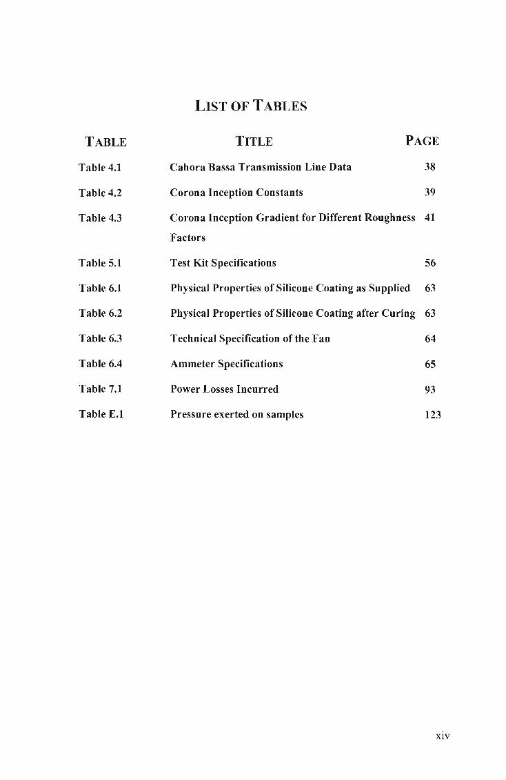
Table 4.1 Cahora Bassa Transmission Line Data 38

Table 4.2 Corona Inception Constants 39

Table 4.3 Corona Inception Gradient for Different Roughness 41

Factors

Table 5.1 Test Kit Specifications 56

Table 6.1 Physical Properties of Silicone Coating as Supplied 63

Table 6.2 Physical Properties of Silicone Coating after Curing 63

Table 6.3 Technical Specification of the Fan 64

Table 6.4 Ammeter Specifications 65

Table 7.1 Power Losses Incurred 93

Table E.1 Pressure exerted on samples 123

XIV

CHAPTER!

INTRODUCTION

1.1 BACKGROUND AND RATIONALE

Corona performance is one of the more important criterion when it comes to the

design and construction of a transmission line. The high voltages at which modem

transmission lines operate have increased the corona problem to the point to which

they have become a concern to the power industry. Consequently, these lines are now

designed, constructed and maintained so that during dry conditions they will operate

below the corona-inception voltage, meaning that the line will generate a minimum of

corona-related phenomena. In foul weather conditions, however, water droplets, fog

and snow can produce corona discharges. With the advent of line compaction, more

time will have to be spent on determining the corona performance of the conductors to

be used on that specific line, as under normal operating conditions the conductor

surface gradient will be very close to the corona inception gradient for that specific

conductor.

It therefore becomes clear that a tool, which can either predict the corona performance

of a future line or generate corona data, which can be used in the design of a new line,

would be invaluable. Several such tools exists, a corona cage is one such tool.

Corona cage tests are often used as a convenient and inexpensive means of obtaining

the excitation functions defining the corona performance of AC conductor bundles,

which in turn is used to predetermine the corona performance of a proposed AC

transmission line design using the same conductor bundle. The main requirement is

that the surface electric field and adjacent electric fields existing in the vicinity of the

conductor bundle are accurately replicated when using the corona cage for testing.

Due to differences in space charge conditions existing between AC and DC

transmission lines, with respect to the presence of corona on the conductors, corona

on conductors under DC in cage conditions is not properly understood as yet.

1

Conductor corona perfonnance (including Corona loss, Radio interference and

Audible noise) as mentioned, is an important criterion when it comes to the design

and construction of transmission lines. On Eskoms only HVDC line (The Cahora

Bassa line), the losses incurred are not clearly known as yet. The design, construction

and testing of a small corona cage will help in quantifying and ana1yzing these losses.

The research for this thesis was conducted in such a manner that on completion, the

following questions have been answered:

• What size cage should be used to accurately model field effects on the Cahora

Bassa Line?

Under this question the following questions arise:

• Will it be feasible to design a corona cage to test conductor bundles?

• What should the length and radius of the cage be?

• Is a corona cage under DC conditions an accurate representation of corona effects

on the line itself?

• What effect will the space charge phenomenon have on the fields in the cage?

• How does changing the surface condition of the conductor affect corona

perfonnance in a cage?

Once this project has been completed it is expected that Eskom will have a better

understanding of DC corona perfonnance. Technological expertise with regards to

HVDC will be available within the confines of Eskom itself. As it is known that

HVDC transmission will greatly increase in the next ten to twenty years, this expertise

will greatly assist Eskom in the design of future HVDC lines as well as improving its

current HVDC line (The Cahora-Bassa line) .

A working HVDC laboratory has been established at the University of Durban

Westville a fonner disadvantaged university in South Africa. This laboratory contains

a small corona cage designed to allow corona to be studied under DC and AC

conditions. This makes small-scale fundamental corona research possible at both

undergraduate as well as postgraduate level. It will also be utilized by industry

wishing to do corona research.

2

1.2 STUDY PROCEDURE

These are the procedures that were followed in order to complete this research.

• A literature survey was carried out which served as the foundation to my

knowledge on corona and corona cages.

Here the (Electrical Power Research Institute) EPRI books were thoroughly

studied and assimilated. This was carried out at Megwattparks' as well as the TSI

library in Gauteng

• Contact was made with vanous entities that have HYDC knowledge and

expertise.

This was done in an effort to establish what work has been done with respect to

corona studies under DC conditions.

• Visits to corona cages were undertaken.

A visit to the Stellenbosch corona cage as well as several visits to Eskom's corona

cage at Megawatt Park was undertaken.

• Design data of the towers and conductors used was obtained from the Cahora

Bassa line.

This was used to calculate the various parameters required for accurate modeling

III a corona cage.

• Electric field calculations were performed to determine the dimensions of the

corona cage to be used. The optimum cage size and conductor configuration

design was thus found.

• Tests were performed III the HYDC laboratory at the University of Durban

Westville. This was done under the supervision of Professor Nelson Ijumba and

Mr. Tony Britten.

• Simulations of the fields were also done using computer software packages.

This complimented the field calculations as well as the test results.

The literature that was reviewed covered the following topics:

• The use of corona cages for AC and DC conditions.

• Field effects on AC and DC lines.

3

• AC and DC corona cage design criterion.

• The effects of corona on AC and DC lines.

• Simulation of corona on DC lines using software packages.

• Radio interference on AC and more specifically DC lines.

• Audible noise levels on HV transmission lines with the emphasis on DC lines.

The following references have proven to be the most useful with regards to this

research:

• IEEE Transactions on Power Apparatus and Systems

• EPRI Transmission Line Reference Book.

• EPRI HVDC Transmission Line Reference Book.

4

CHAPTER 2

CORONA

In this chapter the phenomenon of Corona is discussed.

• Corona: Corona is discussed under general AC conditions and then more

specifically under DC conditions. Various corona modes as well as corona

formation and mechanisms are presented.

• Corona Loss: Corona loss is expounded. The corona loss on AC and DC lines

will be compared to each other. The factors which influence corona losses arfe

discussed with specific attention being given to the factors influencing DC corona

losses.

• Radio Interference: Radio interference is defined. The differences between AC

and DC radio interference are discussed. The levels of RI on the Cahora Bassa line

are stated.

• Audible Noise: Audible Noise will be discussed and defined. Differences between

AC and DC audible noise levels will be discussed.

2.1 CORONA

The environmental effects produced by corona discharges on conductors play an

important role in the design and operation of high-voltage transmission lines. Corona

Loss (CL), Radio Interference (RI) and Audible Noise (AN) are the principal

environmental consequences of corona on both AC and DC lines, while corona

generated space charge environment is also important in the case of DC lines.

In layman's terms corona can be described as the faint glow on the surface of

electrical conductors under high voltages. This glow is caused by electrical discharges

that occur when the electric fields strength on the surface of the conductor exceeds the

electrical breakdown strength of air.

According to the IEEE Standard Dictionary of Electrical and Electronic Terms,

corona is described as: " A luminous discharge due to ionization of the air

5

surrounding a conductor caused by a voltage gradient exceeding a certain critical

value."

Corona discharges form at the surface of a transmission-line conductor when the

electric-field intensity on the conductor surface exceeds the breakdown strength of air,

which is about 30 kV fcm at standard temperature and pressure levels. This occurs

when the conductor surface has irregularities, such as conductor nicks, air-borne

particles (insects, weed and grass seeds, dust, etc.), or water-drops, all of which

enhance the local electric field. This breakdown strength is controlled by a host of

various conditions such as [11, 169]:

• Air pressure

• Electrode material

• Presence of water vapor

• Incident photo ionization

• and Voltage

Corona on power lines is mainly a statistical phenomenon. Scratches, displacement of

strands, water droplets and dirt can cause corona discharges to start at a considerably

lower surface gradient than that determining breakdown in air. Any irregularity on a

conductor's surface causes a voltage gradient concentration that may become the

point source for a discharge. The result of this breakdown of air in this region

generates the following:

• Light

• Audible noise

• Radio noise

• Conductor vibration

• Ozone and other by products.

Generally, corona on high voltage (RV) lines causes losses, interference with

telecommunication lines and radio receivers in the vicinity of the lines. For the

purposes of this study, only Radio Interference, Audible Noise and Corona Loss will

be considered. Pictures of corona activity are shown in figures 2.1 to 2.3.

6

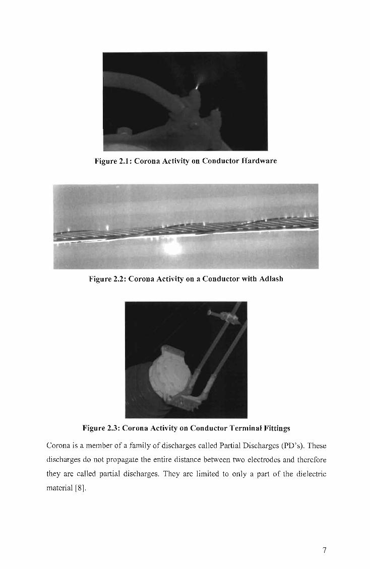
Figure 2.1: Corona Activity on Conductor Hardware

Figure 2.2: Corona Activity on a Conductor with Adlash

Figure 2.3: Corona Activity on Conductor Terminal Fittings

Corona is a member of a family of discharges called Partial Discharges (PD's). These

discharges do not propagate the entire distance between two electrodes and therefore

they are called partial discharges. They are limited to only a part of the dielectric

material [8] .

7

2.1.1 Basic Ionization Processes

If the levels of conductor surface electric fields are high enough, complex ionization

processes take place in the air surrounding the high voltage transmission line

conductors which results in the discharge known as corona.

Atmospheric air is the most important insulating material used on high voltage

transmission lines. Although insulators are used for structural support, ambient air is

the main insulating medium between high voltage conductors and their grounded

support structures and the ground plane.

Atmospheric air consists mainly of water vapor and a number of gasses [4, 55]. The

volume percentage of this water vapor depends on the ambient temperature and is

highest at the equator and decreases towards the poles. The volume percentage of the

gaseous content of dry air remains the virtually the same from part of the earth to

another [4, 55].

Under normal conditions, the gaseous and water vapor molecules in air are electrically

neutral, that is no electrons are either removed from or added to them. Naturally

occurring phenomena however, prevents the air from staying electrically neutral.

These phenomena are: [4, 56]

• Gamma rays produced by radioactive decay processes in the soil.

• Cosmic radiation

• Ultra-violet light.

2.1.1.1 Ionization and Excitement

An atom consists of a nucleus of neutrons and protons, surrounded by electrons in

orbital motion. The number of electrons, which equal the number of protons in the

nucleus, is different for each element. The number of neutrons in the nucleus

determines the atomic mass of the element. The electrons occupy different orbits,

characterised by different permissible energy states. The highest energy of the atom is

found when the electron is in an orbit furthest from the nucleus and the lowest energy

is found when the electron is in an orbit nearest the nucleus.

If enough energy is imparted on the atom to allow the electron in the outermost orbit

to jump to the next permissible higher energy level, the atom is said to be excited. If

enough energy is imparted on the atom so that the orbiting electron is dislodged

8

sufficiently far away from the atom, so that it will not return to its original state, then

the atom is said to be ionized. The energy required for this ionization of an atom may

be supplied in a number of ways. Depending on the amount of energy transferred, the

atom may be either excited or ionized as described by the following equations: [4, 57]

A + e ~ A* + e {Excitation}

A + e ~ A+ + e + e {Ionization}

In actual gas discharges, the electron energy distribution has to be taken into account

in order to get an estimate of the process of ionization by electric collision. In view of

this, Townsend defined a Coefficient (a) as follows:

This is defined as the number of ionization collisions that take place during a unit

length movement of one electron. [17, 23]. This is sometimes referred to as

Townsend's first ionization coefficient. From the above definition the following

differential equation can be derived.

dn = n(x)·a·dx

Where: dn is the number of new electrons freed.

n(x) is the number of electrons.

dx is the distance travelled.

Solving this equation over the distance between the electrodes gives the following

solution.

n = no ' exp(ax)

Where: no is the number of electrodes at the negative electrode.

The solution shows that the number of positive and negative Ions Increases

exponentially. This type of discharge is called an avalanche.

The coefficient ex, changes with field strength, gas pressure and other conditions that

influence the production of electron pairs [11, 170].

Ionization by positive ion impact is an improbable process except at energies much

higher than those likely to be encountered in corona discharges. The energy required

for excitation or ionization may also be derived from electromagnetic energy in the

form of light, or from a photon with an energy level of hv where v is the frequency of

9

radiation and h is Planck' s constant. Photo-excitation and photo-ionization may be

described by the following equations.

A+hv ~ A· (photo-excitation or photon emission)

(photo-ionization)

Ionization by electron collision as well as by absorption oflight play important roles

in corona discharges. Other processes such as thermal ionization and shock ionization

also occur, but do not affect corona discharges.

The ionization phenomenon is the major contributor to the corona power loss process.

When discussing this phenomenon, two zones of activity must be defined. The first is

the ionization zone, which is a very thin circumferential layer surrounding the

conductor surface. The second zone encompasses the electrode and inter-electrode

space and the region between each conductor and the ground plane. Within the

ionization zone the high field strength causes high velocity particles to collide with air

molecules. These collisions cause the Townsend's coefficient of ionization (a) to

exceed the coefficient of electron attachment (11). Electrons are therefore removed

from the atomic structure of the air molecules and are accelerated away from the

negative conductor and toward the positive conductor. These high-velocity electrons

then collide with other air molecules releasing additional electrons in an avalanche

process. Ionization of air molecules occurs during this process. Ions carrying the same

charge as the adjacent conductor are repelled from the ionization zone at initial

velocities of about 1.4 cmls for positive ions and 1.8 cmls for negative ions for every

V/cm of field strength [12, 18].

2.1.1.2 Electron Emission from Conductor Surfaces

Electron emissions from conductor surfaces is an important factor in gap discharges,

especially in corona discharges in air. The electrons at the peripheral layer of atoms

on the metal surface are free to move within the metal. These electrons must gain

sufficient energy, however, in order to escape from the metal surface. [4, 60].

The energy needed to facilitate electron emission from a conductor surface may be

supplied by different physical mechanisms, the more important of which include:

• Thermionic emission;

• Electron emission by positive ion impact;

1f\

• Field emission;

• Photo-electric emission.

Thermionic emission occurs at very high temperatures and is important in vacuum

tubes. Field emission occurs at very high values of surface electric field and is

important mainly in vacuum breakdown phenomena. Both these mechanisms do not

play a role in gas discharges at normal atmospheric pressure and temperature.

2.1.2 Discharge Phenomenon

The basic ionization phenomenon which has been described in the preceding sections

will be useful in understanding the various discharge phenomenon which occurs in

gases.

Figure 2.4 shows a uniform electric field arrangement. A voltage, D is assumed to be

applied between the electrodes, which are separated by a distance d, this produces an

electric field ofE = Did.

At the cathode, free electrons are produced either by natural ionization processes or

by artificial illumination with ultraviolet light. [4, 65].

HV

Figure 2.4: Gas Discharge in a Uniform Field Electrode Arrangement [4]

As the voltage is increased, the typical voltage current curve shown in figure 2.5 is

obtained. This can be divided into three regions as follows [4]:

• For a voltage below Do, the current increases, in a linear fashion, with the voltage

in the beginning and then it saturates gradually as it approaches Do. At lower

voltages the current is produced by the movement of the free electrons, created

either naturally or artificially, due to the electric field in the gap.

11

• As the voltage increases to a level above Uo, the current starts to increase

exponentially. This current increases occurs as a result of the electrons gaining

sufficient energy from the higher electric field in the gap to ionize the neutral gas

molecules and create new electron-positive-ion pairs. These newly created

electrons also gain sufficient energy to ionize other gas molecules, leading to a

process known as cumulative ionization. This exponential rise in the number of

electrons is known as an electron avalanche, this is shown in figure 2.6.

• Above a voltage U j , the current increases very rapidly until flashover or electrical

breakdown occurs at the voltage U2• This rapid increase in the current is attributed

to a process known as secondary ionization, which creates additional electrons at

the cathode capable of initiating new electron avalanches.

Self sustained discharge

Sustained discharge

o

Figure 2.5: Voltage-Current Characteristic of the Discharge [4]

2.1.3 Corona Modes

Corona modes can be categorized into positive and negative polarity modes. For DC

conditions, the conductor will exhibit either the negative or positive mode, depending

on its polarity.

For the same polarity, corona can manifest itself in one or more modes depending on,

the voltage applied, electrode shape and surface conditions. Each of these corona

modes has different characteristics like, current shape, magnitude and frequency of

pulses.

12

2.1.3.1 Negative DC Corona Processes

When the stressed conductor is at a negative potential, electron avalanches are

initiated at the cathode and develop in a continuously decreasing field towards the

anode. Free electrons which, can move much faster than ions in an applied field, are

thus concentrated at the tip of the avalanche. A concentration of positive ions thus

forms in the region of the gap between the cathode and the boundary surface So [4,

67]. This is seen in figure 2.6.

\

\

\ ,

I' () '--____ -=:..

Figure 2.6: Electron Avalanche at the Cathode [4, pg 68]

As can be seen from figure 2.6 free electrons continue to migrate across the gap.

Beyond the surface So the free electrons quickly attach themselves to the oxygen

molecules to form negative ions, which due to their low drift velocity accumulate in

the gap beyond So. Once the development of the first electron avalanche has been

completed there are two ion space charges in the gap as shown in figure 2.7.

E

E

I

J

, \ , \ -

~"-~ +----\. . \; - - ~

.. _;' : : -- :1-:.',:::-I

I I

ED '---_ _ ---'---=:::... I

Figure 2.7: Space Charge Following Completion ofthe First Avalanche [4, pg 68]

l3

From figure 2.7 it can be seen that the ion space charges in the gap produces a slight

increase in the field near the cathode and a corresponding increase in the field towards

the anode. A reduction in the field occurs in the middle of the gap. The effect of the

space charge is such that it actually conditions the development of the discharge,

producing three different modes of corona discharge with distinct electrical, physical

and visual properties [4, 68] .

These modes in order of increasing field intensity are [4, 69]:

• Trichel pulses

• Negative pulseless glow discharge

• Negative streamer discharge.

Trichel Streamer Discharge:

This discharge mode follows a regular pulsating pattern in which the streamer is

initiated, develops and is then suppressed. A short dead time follows before the cycle

is repeated. The duration of an individual streamer is short, about a few hundred

nanoseconds, while the dead time varies from a few microseconds to a few

milliseconds or more. The resulting discharge current consists of regular negative

pulses of small amplitude and short duration, succeeding one another at the rate of a

few thousand pulses per second. The streamer repetition rate is basically a function of

the applied field. It increases linearly with the applied voltage. At high electric fields

however the pulse repetition rate is reduced as a result of the establishment of a short

duration stable discharge system [4, 69].

Figure 2.8: Trichel Streamer Discharge [4,69]

Negative Pulseless Glow Discharge:

If the voltage is now increased further, trichel pulses, after reaching a critical

frequency, change over into a new mode of corona called a pulseless glow. The shift

14

is accompanied by a change in the visual manifestation of the discharge. The

wandering of the discharge on the cathode terminates and it becomes fixed at one

point. Pulseless glow corona exhibits typical features of a glow discharge. It is easily

distinguishable by a bright spherical negative glow followed by a luminous conical

positive column stretching outward from the point. The different parts of the

discharge are separated by two dark spaces [4, 70]. With an increase in the voltage,

the steady corona current increases continuously until, close to breakdown, it changes

back to negative streamers.

Figure 2.9: Negative Pulseless Glow [4, 70]

Negative Streamers:

As the voltage increases further, Negative streamers appear. The conical positive

column reaches out with little branching. The current consists of pulses superimposed

on a quasi-steady state current. The rise times of these pulses are in the order of

0.5*10-6s. The glow discharge characteristics observed at the cathode imply that this

corona mode also depends largely on electron emission from the cathode by ionic

bombardment while the formation of the streamer channel characterized by intensive

ionization denotes even more effective space charge removal by the field [4, 71].

Figure 2.10: Negative Streamer [4,71]

15

2.1.3.2 Positive DC Corona Processes

When the stressed electrode is positive in polarity, the electron avalanche is initiated

at a point on the boundary surface So and develops, in a continuously increasing field

towards the anode. This is shown in figure 2.11 below.

/ ~ ' J" '~ ~

Figure 2.11: Avalanche Development Near Anode [4,71]

This causes the highest ionization activity to occur at the anode. A positive ion space

charge is left behind along the path of development of the avalanche, once again due

to the lower ion mobility. Since there is a high electric field intensity near the anode,

the effect of electron attachment is less than in negative corona, and the majority of

free electrons that are created, are absorbed in the anode. Negative ions will be

formed mainly away from the anode in the low field region.

Due to the presence of the positive ion space charge near the anode, a field

enhancement in the gap is produced. This can be seen in figure 2.12. Photons released

by excited molecules in the primary avalanche give rise to secondary electrons, which

are accelerated in the enhanced field region and create secondary avalanches [4, 72].

This promotes radial propagation of the discharge in the gap, along a streamer

channel.

There are four different corona discharge modes, each having distinct electrical,

physical and visual characteristics which can be seen at the anode prior to the

breakdown of the gap.

These modes in order of increasing field intensity are [4, 72]:

• Burst Corona

• Onset Streamer discharge

16

• Positive Glow discharge

• Breakdown Streamer Discharge

superfiCia'7ading ~~b",Sl corona

+

E

-: . ~. ; .. , . - - ~ "-. .' Radial streamer

development

, , , "

r

Figure 2.12: Successive Stages of Avalanche Development Near Anode [4,72]

Burst Corona:

This discharge results from the ionization activities at the anode surface. These

activities allow the highly energetic incoming electrons to lose their energy before

their absorption by the anode. Positive ions are created, during this process, in the area

directly next to the anode. They build up cumulatively and form a positive space

charge that suppresses the discharge. The discharge current, which results from this,

consists of small positive pulses, each corresponding to the spread of the ionization

over a small area of the anode, and its ensuing suppression by the positive space

charge produced [4, 73].

Figure 2.13: Burst Corona [4, 73]

Onset Streamer Discharge:

This mode of corona discharge results from the radial development of the discharge.

The positive ion space charge formed adjacent to the anode surface causes, field

17

enhancement in its immediate vicinity and attracts subsequent electron avalanches. A

streamer channel develops in the radial direction, which results in the onset streamer

discharge. Onset pulses appear as streamers in a stem with some branching. They

have a high branching repetition rate, which gives them a brush-like appearance.

During the streamer development a considerable amount of space charge ion is

formed in the low field region. The successive electron avalanches results and

absorption of free electrons at the anode results in the formation of space charge in

front of the anode. The electric field at the anode drops below the critical value for

ionization and causes the suppression of the streamer discharge. In order for the

applied field to remove the positive ion space charge and to restore the conditions

necessary for the development of a new streamer, a dead time is required. As this

discharge, develops in a pulsating mode, it produces a positive current pulse of large

amplitude and relatively low amplitude [4, 73].

Figure 2.14: Onset Streamer [4, 74]

Positive Glow Discharge:

In this mode, ionization activity over the anode surface results in a thin luminous layer

immediately adjacent to the anode surface, where intense ionization activity takes

place. The discharge current is mainly a direct current. Over this current a small

pulsating current component with a high repetition rate is superimposed. The

development of this type of discharge can be interpreted as being a result of a

particular combination of the rate of removal and creation of positive ions in the gap.

The positive space ion is renewed from the anode, thus promoting surface ionization

18

activity. The negative ions mainly contribute by supplying the necessary triggering

electrons to sustain ionization activity at the anode [4, 74].

Figure 2.15: Positive Glow [4, 75]

Breakdown Streamer Discharge:

Breakdown streamers resemble onset streamers, but they get displaced from the axial

position by the negative space charge. Positive streamers have velocities, which range

from 20 to 20000 cml/-ts. These streamers advance much faster than negative

streamers due to photo ionization. The streamer discharge rise times are usually in the

nanosecond range. The development of a breakdown streamer is directly related to the

effective removal of the positive space charge by the high field intensity [4, 75].

2.1.3.3 AC Corona Modes

The electric field at the highly stressed electrode, the conductor, varies continuously

with time, both in intensity and polarity under alternating voltages. Different corona

modes occur in the same cycle of applied voltage. The corona mode, which occurs,

can be easily identified by the discharge current.

For short gaps the ion space charge is created and absorbed by the electrodes in the

same half cycle. The same corona modes that develop near onset voltages can be

observed in the two half-cycles [4, 75].

• Trichel streamers

• Positive onset streamers

• Burst corona

For long gaps, the ion space charge created in one half cycle is not absorbed by the

electrodes, but is drawn back to the region of high field intensity in the following half

cycle and can influence the development of the discharge.

19

On practical conductors with a large diameter, it is more common to see, during the

positive half cycle, onset streamers than the glow discharge. On very thin and clean

wires only the glow mode of corona, sometimes referred to as ultra corona, occurs.

This phenomenon has been exploited to obtain higher breakdown voltages of air gaps.

Studies have been carried out on stranded conductors which were wrapped with

thinner wires to eliminate pulsative corona and therefore reduce problems of RI and

AN [4, 76].

2.2 CORONA Loss

The literature on corona loss goes back to the beginning of the century, if not earlier.

Corona loss is a power loss that occurs as a result of corona current that flows from

the conductors of one polarity to the conductors of the opposite polarity or to ground.

The power transmission efficiency of a transmission line is decreased by corona loss

since it adds to the resistance loss (RI2) caused by the load current. [10, 3-149] Corona

loss occurs only when there is corona activity on the transmission line or electrical

conductor that is being considered. However the selection of conductor parameters is

rarely affected by corona loss as, it is generally only a small fraction of the (RI2)

losses. In absolute values however, corona loss can be extremely high. For example

an average yearly loss of about 25 W /m can be expected for a ±500 kV line. In the

case of the Cahora Bassa line, which is about 1400km long, the losses incurred due to

corona loss will be 35 MW per year.

2.2.1 Factors Influencing Corona Loss

In 1956 it was discovered that airborne substances such as insects, dust, vegetation,

spider webs, bird droppings and other non-metal materials and not the imperfections

on conductors as generally assumed, that produced fair weather corona loss on high

voltage lines.

If care is taken to prevent the conductor being scratched during stringing, fair weather

corona discharges are seldom experienced, except on non-metal projections on the

line, after about one year of weathering. The metal protrusions, which remain after the

first year, will produce only the glow type of corona discharge at or below the system

operating voltage [11, 180].

20

Discharges can also occur when a small foreign particle like a speck of dust or

snowflake or raindrop passes the conductor and initiates a discharge from conductor

to particle. The discharge normally starts before the particle comes in contact with the

conductor. This leads to an increase in corona loss.

The effect of water on conductor corona performance is quite significant. Water in the

form of rain or drizzle, forms small drops on the upper surface of a conductor it comes

in contact with. After some time the water runs down the strands forming a layer of

water around the conductor. This eliminates many smaller drops on the top and leaves

suspended drop at the bottom. As the water accumulates, drops will eventually form

on the bottom and fall off due to gravity [11, 181].

Two extreme conditions may exist with regards to the degree of wetness that occurs

on a conductor. They are:

• Hydrophilic

• Hydrophobic

If a surface is hydrophilic it implies that the surface "allows" the water to spread

uniformly over it. On the other hand a hydrophobic surface would cause the water to

bead up in small droplets, similar to water on a waxed surface.

Hydrophobicity has the effect of increasing the surface tension between the conductor

and the water droplets. Local points of electric field intensification occur around these

water droplets formed. This has the effect of decreasing the corona inception gradient

and increasing corona loss.

The hydrophilic condition will decrease the surface tension between the conductor

and the water. This leads to a decrease in electric field intensity around the water

droplets and consequently a decrease in corona loss.

2.2.2 Differences Between AC and DC Corona Loss

Corona current of an HVDC line is dependent on line geometry; particularly pole

spacing, this is as a result of the space charge. For an HV AC line, the corona loss is a

function only of the conductor dimensions and of the corona-free surface gradient.

This means that a change in the surface gradient on AC conductors has the same

effect on the AC corona loss whether it is achieved by changing the voltage or by

21

changing the phase spacing. For HVDC lines on the other hand, the corona loss

depends also directly on the pole spacing even if the corona-free conductor surface

gradient is kept the same. In fact, a pole spacing that increases the corona-free surface

gradient to the same value as an increase in the voltage has more of an effect on

corona loss.

Another important difference between HV AC and HVDC corona loss is the change in

loss due to the weather conditions. For example, 345 kV and 500 kV AC lines have

negligible corona loss in fair weather; foul weather corona loss can be 100 or more

times greater than fair weather corona loss [10, 3-150; 1]. On the other hand, fair

weather DC corona loss is not negligible; but the increase in loss in the passing of

weather conditions from fair weather to foul weather may not be as dramatic as for

AC. It has been noted in some cases that foul weather DC corona is only 2-3 times

larger than fair weather DC corona. [10, 3-150; 1]. Other tests have shown that the

mean foul weather losses are 2-4 times more than fair weather losses [12, 19].

2.2.3 Factors Influencing Corona Loss on DC lines

Under both unipolar and bipolar operating conditions, conductor polarity has little

significant effect on the corona losses incurred. The main differences occur under fair

and rainy weather conditions.

The atmospheric variable with the largest impact on the corona loss is wind flow.

Tests have shown that wind flowing perpendicular to the line has the largest effect on

the corona current distribution at ground level, especially under bipolar lines.

Laboratory tests have shown that corona loss increases with magnitude of the

perpendicular component of the wind applied [4, 205]. Tests have shown that wind

can increase the corona loss and RI by between 2 and 4 times [29].

After the creation of an ion by an electron - air particle collision, positive ions could

attain a velocity of as high as 1.4 cm/s and negative ions up to 1.8 cm/s for every

V/cm of field strength [12, 18]. It is known that the electric field strength rapidly

attenuates with distance from the conductor and therefore the ion velocity is decreased

by one or two orders of magnitude. Typical wind velocities are in the same range and

will thus tend to move ions from the electric field lines, thus inducing a random

dispersion of charged particles downwind from the line.

22

The wind will also remove ions from the ion cloud that forms around the energized

DC conductor at gradients above corona onset. Under no wind conditions this ion

cloud has the effect of creating a stable atmosphere around the conductor. The

formation of this ion cloud of the same polarity around the conductor causes a

suppression of further ion formation at the conductor surface. The wind, which

removes this ion cloud, will move some of these ions to the opposite polarity field

surrounding the other conductor. As a result of this the ion balance is disturbed and

the conductor produces more ions in an attempt to restore the equilibrium.

As wind velocities increase, more ions are moved away from the conductors this

causes, the corona current and the corona losses to increase [12, 31].

The effects of wind in corona cage conditions will be tested and documented in

chapter seven.

2.3 RADIO INTERFERENCE

2.3.1 Definition of Radio Interference

One of the consequences of transmission line corona discharges is radio interference.

Radio interference is a rather general term, which, by definition, refers to any

unwanted disturbance within the radio frequency band, such as undesired electric

waves in any transmission channel or device. This is also known as radio noise.

Pulses of current and voltage are produced on transmission line conductors by corona

discharges, which are pulsating in nature. These pulses are characterized by rise and

decay-time constants, in the order of a few nanoseconds to tens or hundreds of

nanoseconds, and by repetition rates, which may be in the MHz range. As a result of

this, the frequency spectra of these pulses can cover a considerable portion of the

radio frequency band. The electromagnetic fields resulting from the corona discharges

may, therefore, create unwanted disturbances in the operation of a transmission

channel or device over a wide range of frequencies.

In theory transmission line radio interference can interfere with any radio frequency

communication. This is dependent on factors such as, the distance from the

transmission line to the communication-receiving device, the orientation of the

receiving antenna, the transmission line geometry, and the weather conditions. The

23

level of interference may be such that the reception of the desired information is

practically unaffected; or it may be such that reception is rendered completely

unintelligible; or, it may range between these two extremes.

2.3.2 Differences Between AC and DC Radio Interference

Much radio interference research has been devoted to AC transmission lines and the

design considerations for AC are similar to DC, however there are a few important

differences.

Under AC conditions the highest levels of RI occur during wet weather conditions.

Under DC conditions the highest RI levels occur during fair, dry weather. During wet

weather conditions rain drops on the surface of the electrical conductors cause local

field enhancements, due to their shape. This produces corona at electrical fields,

which are much lower than the conductor electric field that exists in corona free

conditions.

As a result of this there is an intense ionization of the air near the surface of the DC

conductor and a large amount of space charge is produced. Due to this space charge

there is an increase in corona loss and air ions. Space charge also has the effect of

producing a fairly uniform ion cloud around the conductor and of maintaining the

conductor surface electric field at the value of the rain - drop corona onset field.

Raindrop corona is not very impulsive under the above conditions, compared to most

corona in fair weather conditions. This type of corona is more of a glow. Glow corona

corresponds to steady noiseless charge emission from conductors into space. This

does not occur on AC lines, due to the nature of the alternating electric field on the

surface of the conductor that prevents the formation of a uniform ion cloud of the

same polarity. As a result of this phenomenon, RI generation on DC lines is higher in

fair weather than in wet weather [4].

The positive pole of a bipolar DC line produces more RI than the negative pole to

such an extent that the RI produced by the negative pole can be ignored. This implies

that, whereas AC-RI occurs on all conductors, DC-RI is limited to specific

conductors. The reason for the positive pole producing more RI than the negative pole

lies in the fundamental differences in the corona processes, which occur at these

poles. Current pulses caused by corona have higher magnitudes and longer decay

24

times on a positive polarity conductor than on a negative polarity conductor.

Consequently, corona on the positive polarity affects broadcast bands more than the

negative pole [4]. Figure 2.16 below shows the lateral profile of RI under AC and DC

conditions.

,,, >t'

00 00 e 0;

"- <5 0

~o ~o

E E

;; ;; 40

40 ::. "- ~ - cc ::::l

'" '" ;0 30 I

c;,:; oe:

a) 20 I b) ,0

10 10

! 0 1 0

I .,

-lOO - 7~ - ~o - ::~ 1~ ~ '5 lOO - lOO -:~ • SO - : ~ 2 ~ so ..... 100

Distance. m DlsJance, m

Figure 2.16: Lateral Profile of RI: a) AC, b) DC [4]

The measured levels of RI on the Cahora Bassa line are as follows:

• Negative Polarity 350 kV = -65 dBm.

• Positive Polarity 350 kV = -70 dBm.

These levels were measured on the shield wire of the Cahora Bassa line, using a

Wandel and Golterman selective voltmeter.

2.4 AUDIBLE NOISE

2.4.1 Causes of Audible Noise

The Audible Noise (AN), emitted from high-voltage lines is caused by the discharge

of energy that occurs when the electrical field strength on the conductor surface is

greater than the 'breakdown strength' (the field intensity necessary to start a flow of

electric current) of the air surrounding the conductor. AN can also be produced by

intermittent flashovers of insulators in transmission line insulator strings.

AN from transmission lines, which is corona generated is very different from other

environmental noises to which the public may be exposed to. Compared to traffic and

aircraft noises, AN levels are generally lower but cover a much wider frequency

25

spectral range. The AN frequency spectrum also varies in level and shape depending

on the weather conditions.

2.4.2 Differences between AC and DC Audible Noise

DC lines have the highest levels of AN under fair, dry weather conditions, compared

to AC lines which experience higher AN levels under wet weather conditions. In wet

weather conditions, ionization on DC lines is so high that irregularities on the surface

of the conductor are surrounded by a high amount of space charge, which reduces the

electric field at the conductor surface, as well as reducing the intensity of the corona

current pulses. This results in audible noise generation on DC lines being less during

wet weather than in dry weather.

[10] States: " The audible noise generated by each noise source on the conductor

surface is a function of the characteristics of the source (its corona inception field),

and of the electric field at the source. The electric field at the source, in turn, depends

on the space charge generated by the source itself and by other corona sources that are

nearby. This space charge reduces the electric field at the surface of the conductor

below the nominal (corona-free) conductor surface field. If enough space charge is

produced, the surface field is reduced below the corona inception field of the source

and the source ceases to be in corona, until the space charge is driven by the electric

field sufficiently away from the source. The time between bursts of corona from

HVDC conductors, i.e. the 'relaxation time of HVDC corona' can vary from zero

(practically continuous corona emission) to several seconds. HV AC corona is quite

different from this phenomenon as the surface electric field varies at the applied

frequency. The shape of the sources change due to erosion and dehydration caused by

corona."

HVDC emissions that are almost continuous occur when the corona inception of the

source is significantly lower than the corona free conductor field. In this case the

corona current is either continuous or occurs in small pulses that do not produce

audible noise. This occurs under wet weather conditions when raindrops decrease the

inception field.

All of this means that HVDC AN, is a rather complex function of the nature and

number of corona sources. Both, a source free conductor and a conductor with many

26

sharp (low corona inception field) sources, produces no or very little AN. The worst

conditions occur with a critical number of critical sources per unit length.

The figure below compares the effect of rain on HVDC corona to that on HV AC

corona.

AUDIBLE NOISE

eof!A) AC LINE

I r -..·"..../<-I

50-

30 L-__________ ~ __________ ~ ______ _

f-- faIr - - T..;.I_-- raln----~+--- after raIn ---..

Figure 2.17: Differences Between AC and DC Audible Noise [10].

Once again, the positive polarity pole of a bipolar HVDC line produces more audible

noise than the negative pole. AN generated by the negative pole can be ignored. On

the positive pole pulses, caused by corona, have higher magnitUde and larger decay

times than on the negative polarity.

2.5 SUMMARY

Corona is a result of the voltage gradient, of a conductor or any voltage carrying

equipment, exceeding a certain critical value. This critical value is dependent upon

factors , such as

•

•

•

• •

Air pressure

Electrode material

Presence of water vapor

Incident photo ionization and

Voltage level

The phenomenon of corona results in the generation of various discharges, the main

ones being:

• Light

27

• Audible Noise

• Radio Noise

Corona modes can be characterized under positive and negative polarity modes.

Negative DC polarity modes in order of increasing field intensity are as follows:

• Trichel pulses

• Negative pulseless glow discharge

• Negative streamer discharge

Positive DC polarity modes in order of increasing field intensity are as follows:

• Burst corona

• Onset streamer discharge

• Positive glow discharge

• Breakdown streamer discharge

Different corona modes occur in the same half cycle of applied voltage under AC

conditions. The same corona modes that develop near onset voltages can be observed

in the half cycles, namely:

• Trichel streamers

• Positive onset streamers

• Burst corona

The efficiency of transmission lines is decreased by corona loss, which adds to the RI2

losses incurred by the line. Corona loss is influenced by a host of factors such as

scratches, nicks and airborne substances.

HVDC corona current which, causes corona loss is dependent upon line geometry,

particularly pole spacing, due to the effect of space charge. On RV AC lines however,

corona loss is a function only of the conductor dimensions and the corona free surface

gradient.

AC corona loss is negligible in fair, dry weather conditions while the same cannot be

said for DC lines. AC wet, foul weather losses may be many times higher than the AC

fair, dry weather losses. DC wet, foul weather losses may only be about 2-3 times as

large as the wet, foul weather DC losses.

28

DC radio interference is more severe on the positive pole than on the negative pole. It

is therefore limited to specific conductors only. The highest levels of DC radio

interference occurs during fair, dry weather. The worst AC radio interference occurs

during wet, foul weather conditions.

DC lines also experience the highest levels of audible noise under fair, dry conditions

compared to AC lines that experience higher levels of AN under wet, foul weather

conditions.

29

CHAPTER 3

CORONA TEST METHODS

This chapter describes the various methods, which are employed for corona testing.

There are normally two main objectives for experimental corona studies on

conductors. These are:

• To gain a better understanding of the physical mechanisms involved in corona

discharges as well as the resulting corona effects.

• To generate experimental data that can be used to develop prediction methods

for the corona performance of transmission lines. [4,238]

Since the discovery that conductor size has an influence on the current carrymg

capacity as well as the corona losses, laboratory as well as outdoor test methods, have

been used to study different aspects of corona performance. The main corona test

methods employed are as follows:

• Laboratory test cages

• Outdoor test cages

• Outdoor test lines

• Operating lines

3.1 LABORATORY TEST CAGES

Laboratory studies have been carried out using a variety of electrode geometry's such

as; point-plane, sphere-plane and concentric-spherical, in order to understand the

physics of corona discharges. Studies of corona on cylindrical conductors have been

mostly made in a configuration commonly known as a corona "cage". This

configuration consists mainly of a test conductor placed concentrically inside another

metallic cylinder with a much larger radius. The outer cylinder may be made out of a

thin metallic sheet, but it is often made of some wire mesh. It is due to this wire mesh

that it is called a corona cage.

30

Applying sufficient voltage between the conductor and the cage generates high

conductor surface electric fields. Generally, voltage is applied to the conductor and

the cage is maintained at close to zero potential by connecting it to ground via a small

measuring impedance. In special cases, where fast-rising corona current pulses are to

be measured, this may be reversed with the conductor being grounded and the voltage

being applied to the cage.

The main benefit of the cage setup is that the conductor surface electric field

distribution can be determined quickly and accurately. Early corona research was

mainly carried out in laboratory corona cages. These cages have also been used to

study the basic physics of corona discharges on cylindrical conductors at alternating

as well as direct voltages. Corona characteristics studied in the laboratory include

conditions for the occurrence of different AC and DC corona modes, corona pulse

characteristics such as amplitude, pulse shape, repetition rate etc., corona loss (CL),

radio interference (RI), audible noise (AN) and ozone generation.

For a cage of finite length, the electric field distribution in the longitudinal direction is

uniform over the central section of the conductor and becomes non-uniform towards

both ends. By adding a guard section of the cage at both ends, a central section of the

cage may be selected to obtain a fairly uniform electric field distribution along the

length of the conductor. The central section is used for corona measurements by

connecting it to ground through appropriate measuring impedances. The two guard

end sections will be connected directly to ground.

g In g o ° ,,-0 ________ ~o 0 0

~ 1IIIn O~====c========::iO~

g = guard sections: m = measuring section

c = conductor

Figure 3.1: Electrical Diagram of Corona Cage [4, 239]

An important criterion for the design of any cage setup is to have an adequate margin

between the breakdown and corona onset voltages. For the largest conductor to be

tested the cage diameter should be small enough to obtain corona at a sufficiently low

31

voltage. This is due to the fact that the largest conductor in the cage will result in the

lowest electric field gradient measured for the same applied voltage in the cage as

when compared to a smaller diameter conductor. At the same time the air gap

clearance between the cage and the conductor should be large enough so that the

breakdown voltage is higher than the onset voltage. A margin of at least 50% between

these two voltages permits studies to be carried out at different conductor surface

gradients above corona onset.

Smooth as well as stranded conductors may be tested in laboratory cages. Conductor

surface imperfections and water drops can also be simulated within the laboratory,

using different types of metallic protrusions. Artificial contaminants, such as grease

and sand have been used to simulate low values of conductor surface roughness factor

and to study the corona performance of polluted conductors.

3.2 OUTDOOR TEST CAGES

To test conductor bundle configurations commonly used on transmission lines; the

cage dimensions have to be much larger than what those of laboratory cages are. An

outdoor cage also permits the experimental data collection to be obtained under

natural weather conditions.

Figure 3.2: Outdoor Corona Cage [4]

An outdoor test cage arrangement consists essentially of conductor configurations

placed at the center of a wire mesh enclosure that is either circular or square in cross

32

section. Outdoor corona cages are usually square because of difficulties in fabricating

cylindrical cage enclosures of a large diameter. Conductor lengths in the order of

hundreds of meters are required to properly simulate fair weather corona performance

in cages whereas shorter conductor lengths are needed for to simulate foul weather

corona performance. Outdoor cages have generally been used mainly to determine the

corona performance under heavy rain conditions, by using artificial rain.

3.3 OUTDOOR TEST LINES

Outdoor test lines are essentially short sections of full-scale transmission lines. They

are used to obtain the statistical all weather corona performance of certain conductor

configurations.

For AC corona studies, either three-phase or single-phase test lines can be used. Three

phase test lines accurately reproduce the electric field conditions of normal

transmission lines. Single-phase test lines are relatively less expensive to build and it

is comparatively easier to use the test results for predicting the performance of long

three-phase lines. An example of an outdoor test lines is shown in figure 3.3 below.

The entire inter-electrode region of DC transmission line is filled with space charge,

which has an important effect on corona performance, therefore a single conductor

test line can be used to study unipolar corona while a two conductor test line is

necessary for bipolar corona studies [4].

Figure 3.3: Outdoor Test Line [4]

33

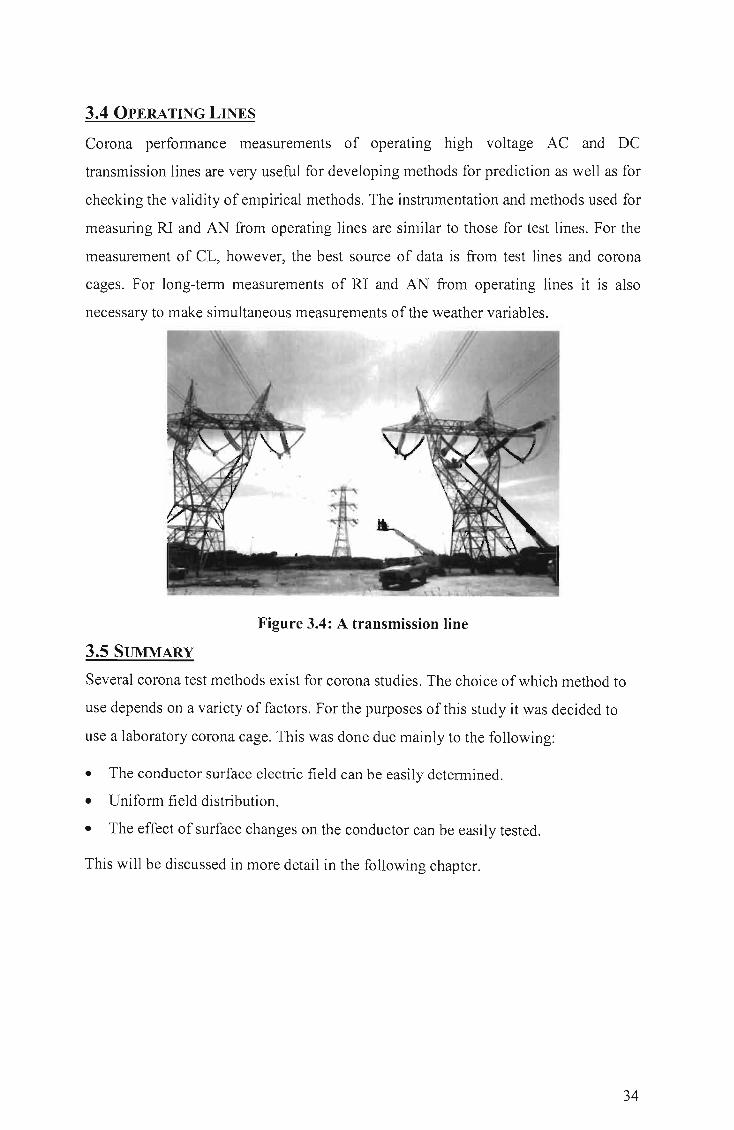
3.4 OPERATING LINES

Corona performance measurements of operating high voltage AC and DC

transmission lines are very useful for developing methods for prediction as well as for

checking the validity of empirical methods. The instrumentation and methods used for

measuring RI and AN from operating lines are similar to those for test lines. For the

measurement of CL, however, the best source of data is from test lines and corona

cages. For long-term measurements of RI and AN from operating lines it is also

necessary to make simultaneous measurements of the weather variables.

Figure 3.4: A transmission line

3.5 SUMMARY

Several corona test methods exist for corona studies. The choice of which method to

use depends on a variety of factors. For the purposes ofthis study it was decided to

use a laboratory corona cage. This was done due mainly to the following:

• The conductor surface electric field can be easily determined.

• Uniform field distribution.

• The effect of surface changes on the conductor can be easily tested.

This will be discussed in more detail in the following chapter.

34

CHAPTER 4

CORONA CAGE DESIGN

This chapter covers the design and construction of the Corona Cage in the High

Voltage Direct Current (HVDC) laboratory.

The criteria used for the design of AC and DC corona cages are discussed. The design

techniques used and associated calculations are presented here. The corona inception

voltage for HVDC lines is discussed and calculated for the Cahora Bassa line.

The criterion used for the design of this specific cage is discussed, as well as the

design techniques and constraints, which were considered during the design and

construction process.

Cages were first built in the 1960's, primarily to study RI and CL. Audible noise only

became an issue in the late 1960's. Ozone became an issue about a decade later. [7]

4.1 ELECTRIC FIELD MODELING

Electric field modeling of the cage and the conductor to be used was done with a

software package called QUICKFIELD©. The corona cage can easily be modelled in

any finite element simulation package, since its symmetrical properties simplify it to a

one-dimensional problem. QUICKFIELD© was used to simulate a corona cage [23].

A very simple model was implemented and used. The results of which can be seen in

figure 4.l. As is expected, the highest field intensity occurs around the conductors'

surface while the lowest intensity occurs near the cage walls. It is this effect which

allows corona studies to take place in a corona cage. We can obtain a very high

electric field gradient on the surface of the conductor by using a relatively low applied

voltage.

35

Strength E (10"v/rn)

27 1

2 ,067

1 .862

1 .658

1 .453

1 . 2 4 9

1 . 0 4 5

. 8 4 0

.636

.4 3 1

.227

Figure 4.1: Electric Field Modeling of Conductor and Corona Cage

Figure 4.2 below shows the electric field model of the corona cage from a side view

with a conductor strung up in the middle. The orange region is the field within the

cage, the blue region is outside the cage. This shows the effect that the guard rings

have on the field distribution in the cage. The ends of the cage shows how the field is

non-uniform in that region, in the center of the cage we see that the field is totally

uniform, with no fringing effects present at all. We only have slight field changes in

the area where the outer rings are attached to the inner ring. These are the little

yellow/green spots on the top and bottom of the orange region.

Figure 4.2: The elimination of the fringing effects on the inner ring

36

4.2 CORONA CAGE DESIGN

The main questions, which have to be answered in the design of a corona cage, are as

follows:

• What SIze cage should be used to accurately model field effects, e.g. on the

Cahora-Bassa Line? Under this question the following questions arise:

• Will it be feasible to design a corona cage to test conductor bundles?

• What should the length and radius of the cage be?

Secondary questions that arise with this specific DC cage are as follows:

• What size cage will be needed under the prevailing conditions, e.g. space

constraints and source voltage limitations?

• What effect will the space charge phenomenon have on the fields in the cage?

4.2.1 Type of Cage

In order to determine what type of cage we need, we have to know the dimensions of

the Cahora Bassa HVDC transmission line. This is shown in figure 4.3.

o o o M M

· ····················· ~r ·

o o t'\0 M

o o N t'M

Figure 4.3: Cahora Bassa Transmission Line Tower (all dimensions in mm).

37

PARAMETER DIMENSION

Minimum Ground Clearance 8.55m

Maximum Sag 16.25m

Spacing at Midspan 11m

Table 4.1: Cahora Bassa Transmission Line Data

Table 4.1 shows the clearances and sag that occurs on the line itself, this information

is necessary for calculating the conductor surface gradients. The Cahora Bassa line

uses a four-bundled conductor configuration. Which can be seen in figure 4.4.

q P R

Figure 4.4: Cahora Bassa Conductor Bundle Configuration

Where: r = Sub-Conductor radius = 1.59cm.

R = Sub-Conductor spacing = 45 cm

4.2.2 Bundled Conductors

Bundled conductors are generally used, instead of single conductors, when the

receiving end has a high power requirement. Bundled conductors, also reduces the

electric field gradient, which a single conductor may experience.

The equivalent radius of bundled conductors is given by the following formula: [11,

22]

R = A ~n.d (4.1) eq 2 A

Where: A is the sub-conductor bundle diameter = ~(2Rr

n is the number of sub-conductors.

d is the diameter of each sub-conductor = 2r.

For the Cahora-Bassa line,

38

n = 4 and d = 3.18cm.

So,

R ~ 63.64 Y4 . 3.18 ~ 21.276cm eq 2 63.64

We can take this value to be 21.3cm.

Peeks formula gives us the corona onset gradient which is independent of applied

voltage:

E =E .m.5[1+~] (4.2) c 0 ~

Where: m = roughness factor (we will assume this to be 0.8 for simplification)

cS = Correction factor also known as Relative Air Density

r = conductor radius in centimeters (Req in this case)

Eo and K are constants.

Constant AC Positive DC Negative DC

Eo (kV/cm) 31 33.7 31

K 0.308 0.24 0.308

Table 4.2: Corona Inception Constants

cS = L. 293 (4 3) 760 (273 + t) .

Where:p = prevailing atmospheric pressure in mm of mercury

t = ambient temperature in degrees Celsius.

So for the Cahora-Bassa line: At 1800m the atmospheric pressure is given by:

So:

1800 760---x 10 = 610mmHg

120

5 = 610 . 293 = 0.789 760 (273 + 25)

And Ec for positive polarity DC can now be calculated as follows :

39

Ec = 33.7.0.8.0.789[1 + -J 0.24 1 = 25.83kV 1 cm 1.59·0.789

This shows that for the particular conductor used the corona inception gradient is

25.83 kV/cm. This value is lower than the breakdown strength of air (which is 30

kV/cm). Under certain conditions this inception gradient may decrease, and then the

line may go into corona.

From Literature [12, 22] we find an equation to calculate the maximum surface

gradient which monopolar lines may experience.

_ 2V(1 + B) kV 1 (4.4) gmax - 2H cm

ndln -R eq

Where: V = voltage of one conductor (kV)

n = number of sub-conductors

d = diameter of sub-conductors (cm)

H= Line to ground clearance (Ave. height)(cm)

B = "influence" of charges on other sub-conductors comprising the bundle or

bundling coefficient

Since the Cahora Bassa line uses a four-conductor bundle,

B = 4.242d (4.5) 2c

Where: c = distance between sub-conductors in cm

d = diameter of sub-conductor in cm

Now:

• B=0.15

• V= 533 kV

• n=4

• d= 3.18 cm

• c = 45 cm

• H = 1497 cm (Height - 2/3 of the sag).

40

The inception gradient is not very close to the maximum operating surface gradient,

so under normal operating conditions the Cahora Bassa line will not go into corona.

However the actual roughness factor could be lower than the roughness factor of 0.8

used to calculate the inception gradient. This would decrease the corona inception

gradient, which could lead to the operating gradient being much closer and even

above the corona inception gradient. The table below gives the inception gradient for

the Cahora Bassa line configuration for various conductor surface roughness factors.

Table 4.3 shows that as the surface roughness factor decreases, so the chances, of the

conductor, going into corona increases. It is important to keep in mind that the

maximum conductor surface gradient that the line will experience under normal

conditions is 19.49 kV/cm. The table shows that if the roughness factor of the

conductor drops to 0.6 or below, the conductor will go into corona.

CONDUCTOR SURFACE CORONA INCEPTION

ROUGHNESS FACTOR GRADIENT

1 32.29

0.7 22.60

0.6 19.37

0.5 16.15

0.4 12.92

Table 4.3: Corona Inception Gradient for Different Roughness Factors

4.2.3 Cage Required to Model Bundled Conductors

The cage diameter required to accurately model corona conditions that occur on the

Cahora Bassa line, can be determined as follows: using the formula for calculating the

gradient of concentric cylinders, which is as follows:

Where: V is the applied voltage

a is the inner radius

(4.6)

41

b is the outer radius

Now making b the subject of the formula we get:

b=a.exp[~] a·E c

Using a = 21.3cm (this is Req for the Cahora Bassa line which was calculated earlier)

and V = 200kV and Ec = 25.83kV/cm (which is the positive corona inception gradient

calculated for the Cahora Bassa line) we find that b = 30.64cm. This means that the

diameter of the cage should be about 62cm.

In order to ensure that the cage accurately models the in-service conditions of the

conductors on the Cahora Bassa line, it is has been said that the corona cage diameter

has to be at least 3 - 5 times the sub-conductor spacing. This means that the cage will

have to have a minimum diameter of 1.35m - 2.25m. As well as having a large

diameter, the length of the cage would have to be about I8m. This length was derived

using the ESKOM corona cage as a reference and scaling according to the diameter.

The length of the cage needs to be sufficient in order to eliminate any fringing, which

may occur, as well as to ensure electric field uniformity along the conductor.

It is interesting to note that the results of the calculations presented above, contradict

the diameter having to be 3 - 5 times the sub-conductor radius. The necessity of

having a large conductor to cage wall distance could be attributed to the phenomenon

of flashover. A large enough spacing will prevent flashovers from occurring. This

was, demonstrated by Tomkins in his thesis [26].

To ensure that a uniform field distribution along the central section of the conductor is

obtained, the length of the cage has to be fairly long, at least 3 - 5 times the diameter.

However with the use of end rings (as discussed in chapter 3), this criterion is greatly

reduced. We can now obtain a uniform field distribution with a much shorter length of

cage.

Due to the weight of the bundled conductors a hydraulic tensioning system would

have needed to be included in the cage design, to ensure that the conductors are

accurately tensioned and strung. This design would mean that the cage would have to

be installed in an outdoor location. Due to space constraints in the laboratory at the

42

University of Durban Westville as well as the cost of constructing such a cage, it was

decided that it was not feasible to further pursue the design of this type of cage.

As the cage needs to fulfill the added role of being a teaching tool, it was more

feasible to design a single conductor cage. If a cage were designed to test bundled

conductors it may not have been accessible to undergraduate students for

experimentation purposes due to the costs and labor intensity of stringing conductors

up in the cage. Due to these factors, a single conductor corona cage was instead

decided upon and designed.

From here on all calculations and designs presented will refer to a single conductor

corona cage. The source voltage was assumed to be 200 kV at sea-level as at the time

of the design, the source voltage was not known, therefore a conservative estimate of

200 kV was chosen.

4.3 ELECTRIC FIELD CALCULATIONS FOR A SINGLE CONDUCTOR

CORONA CAGE

A corona cage that is used for testing a single conductor can be accurately modeled as

a co-axial cylinder. The formula for maximum surface gradient in such a

configuration is the same equation as 4.6 which, is as follows:

Where: v = applied voltage in kV.

a = inner radius in cm.

b = outer radius in cm.

(4.7)

Each conductor will have a different corona inception gradient, which is dependent

upon its diameter r, its surface roughness factor m, and the Relative air density (RAD)

8. Peek's formula gives us the relationship between the corona inception gradient and

these factors.

Peeks formula is as follows: [12]

E, =33.7m.,,{1+ 5;2:) (4.8)

Now assuming m = 0.8 and 8 = 1 (RAD at sea level) and using r = 1.59cm,

43

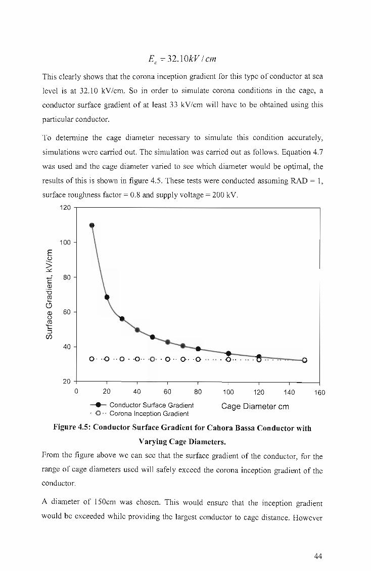
Ec = 32.10kV / cm

This clearly shows that the corona inception gradient for this type of conductor at sea

level is at 32.10 kV/cm. So in order to simulate corona conditions in the cage, a

conductor surface gradient of at least 33 kV/cm will have to be obtained using this

particular conductor.

To determine the cage diameter necessary to simulate this condition accurately,

simulations were carried out. The simulation was carried out as follows. Equation 4.7

was used and the cage diameter varied to see which diameter would be optimal, the

results of this is shown in figure 4.5. These tests were conducted assuming RAD = 1,

surface roughness factor = 0.8 and supply voltage = 200 kV.

120 .---------------------------------------------------~

100

E u

~ ...... 80 c ID "0 co .... (9 ID 60 u ~ ::J

Cl)

40

0 ·· 0 ·· 0 · ·0 ·· ·0 ·· 0 ·· 0 ·· 0 ····· 0 ······

20T-----,------r-----,-----,------r-----.-----.-----~

o 20 40 60

_ Conductor Surface Gradient . 0 ·· Corona Inception Gradient

80 100 120 140

Cage Diameter cm

Figure 4.5: Conductor Surface Gradient for Cahora Bassa Conductor with

Varying Cage Diameters.

160

From the figure above we can see that the surface gradient of the conductor, for the

range of cage diameters used will safely exceed the corona inception gradient of the

conductor.

A diameter of 150cm was chosen. This would ensure that the inception gradient

would be exceeded while providing the largest conductor to cage distance. However

44

the corona cage should also be able to test conductors of different radii. This is to

ensure its viability. A varying diameter cage was also discussed after a visit to

Stellenbosch University's high voltage laboratory where such a cage is in use.

However due to complications with regards to the construction of such a cage a

decision was made to have one with a fixed diameter.

A second test was performed to determine the feasibility of a cage with a diameter of

150 cm. In this simulation the cage diameter and all other values were kept constant,

while the conductor diameter was varied. The graphical results of these simulations

are shown in figure 4.6. The figure shows that a corona cage with a diameter of

150cm can be used to test corona phenomenon on all conductor diameters from O.lcm

up to about 4cm. The conductor surface gradient induced by the cage exceeds the

corona inception gradient for conductors with diameters in the given range. This

ensures that the cage can be used to test most conductors used by ESKOM both for

DC and AC voltages. It should be noted that under DC conditions the conductor will

be monopolar with the cage connected to earth.

350.-------------------------------------------------~

----- Conductor Surface Gradient Conductor Diameter cm . o · Corona Inception Gradient

Figure 4.6: Conductor Surface Gradient for Various Conductors with Cage

Diameter Fixed.

45

It would be possible to test conductors with larger diameters in the cage this would be

achieved by increasing the supply voltage (which can go up to SOOkV) until the

conductor surface gradient exceeds the corona inception gradient for that particular

conductor. All the simulations were based on a supply voltage of 200kV, this was

done so in order to allow for any unanticipated difficulties with exceeding the corona

onset voltage. If any of these occur, the voltage could be increased in order to put the

conductor into corona.

Based on the simulation results, the diameter of the cage was decided upon. Next, the

length of the cage had to be defined. From studying the Stellenbosch cage, it was

deemed feasible to have a cage of similar length, which will be approximately 2m.

Since the length of the cage has to be approximately 2 to 3 times the distance of the

conductor to the cage [27]. This will eliminate any fringing effects at the ends of the

cage. The mounting design of the cage follows the Stellenbosch design quite closely

[26].

It has to be noted that the cage could also be fitted with a sprinkler system, this is so

that the effects of rain on the conductor, both at positive and negative polarity can be

tested and the results documented. The sprinkler system could, possibly be designed

by other students doing corona work in the cage.

To ensure that the cage can be used for testing, through the entire spectrum of service

conditions, which may occur on the line, the maximum surface gradient that the

Cahora Bassa conductor may experience has to be known, this was earlier calculated

to be 32.10 kV fcm. From the simulations presented above it has been shown that this

surface gradient will be obtained within the cage without exceeding the DC source

voltage of200kV, thus ensuring that corona studies may be undertaken in such a cage.

A detailed discussion on the design and construction of the cage and support structure

can be found in Appendix A.

4.4 THE EFFECT OF SPACE CHARGE

Electric fields are vector quantities having magnitude and direction. The space charge

density on the other hand is a scalar quantity having only a magnitude. Space charge

density is essentially composed of two classes of charge carriers i.e.

• Small air ions and

46

• Charge aerosols

The two carriers are distinct due to their mobility and their nature.

4.4.1 Space Charge Behaviour

The behavioral pattern, of the Space charge phenomenon is easily visualized and can

be described in qualitative terms. Near the conductor, small air ions, which are corona

generated, are subject to a force caused by the constant polarity electric fields. These

ions are also subject to convective forces by the wind as they move away from the

line and the electric field due to the line decreases. If the conductor surface gradient

increases, due either to increased voltage or a decrease in the radius of curvature of

the conductor, the corona activity will obviously increase. This increased corona

activity produces more small ions, which fill the region between the electrode and

ground, which increases the electric field and small ion density [6, 696]. When the

applied voltage is above the corona onset voltage, unipolar DC corona in air manifests

itself in the space beyond the ionization layer, as a steady unidirectional flow of

charged particles away from the coronating electrode. The flow of ions is steady and

is determined by the magnitude and direction of the local electric field intensity vector ~

E. The conventional methods of describing DC ionized fields make use of several

simplifying assumptions. They are as follows [5]:

• Ionic mobility'S are constant (independent of electric field magnitude)

• Positive and negative ion mobility'S are equal.

• The diffusion of ions is neglected

• The effect of wind, humidity and aerosols is neglected.

4.4.2 Bipolar and Unipolar Space Charge Effects

There is also a difference between the corona loss performance of unipolar and

monopolar DC lines. On bipolar lines both the positive and negative polarity

conductors, simultaneously present corona activity. Three space charge regions may

be identified in such a case.

• A Positive unipolar region between the positive conductor and ground,

• A Negative unipolar region between the negative conductor and ground

• A Bipolar region between the two conductors.

47

In the bipolar regions, ions of both polarities mix which leads firstly to a reduction in

the net space charge and secondly to a recombination and neutralization of the ions.

This mixture of ions of opposite polarity reduces the effective space charge and

results in a lower screening effect.

In the unipolar region, a screening effect is produced by the space charge present in

the inter-electrode region. Lowering the electric field in the vicinity of the conductor

and consequently reducing the intensity of ionization achieves this. This stabilizes the

discharge activity and limits the corona current [10, 193] .

Therefore, in bipolar cases, the corona current will be higher than in a corresponding

unipolar case, since larger total amounts of positive and negative charges will have to

be emitted to produce the same screening effect. Since corona loss is dependent upon

the corona current, it leads to the conclusion that corona loss is higher in bipolar cases

than in corresponding unipolar cases [4].

4.4.3 Calculation of the Space Charge Effect

From Gauss's Law, the divergence of the electric field intensity E is related to the

charge density p by a constant. Also known as Poisson's equation.

--> p V· E = - (4.9)

E o

Where Eo is the permittivity of free space, a constant. The current density is given by

the following equation.

-->

j=kpE (4.10)

Where, k is the ionic mobility. The divergence of the current density is as follows:

V'j=O (4.11)

Equations, 4.9, 4.10 and 4.11 describe the unipolar ionised field [3, 718-731].

Since the corona cage and conductor can be modelled as coaxial cylinders the

problem can be reduced to a one-dimensional problem, due to the symmetry involved. ~

I.e. the distributions of the potential <p, the electric field E , and space charge p, are

functions of the radial co-ordinate r, only. Figure 4.7 shows the corona cage

configuration. (Not to scale)

48

Figure 4.7: Concentric Co~figuration of Corona Cage

Where:~j = the conductor voltage V.

rj = conductor radius.

~n = cage voltage = QV.

rn = cage radius.

In this geometry the exact solutions of the potential <p, the electric field E ' and space

charge p, within the corona cage for the region R, (rj <R<rn), are known and are given

in the closed form by the following formulae [15].

Where:

q>(+ V -k, . {ffr ) - k, +k, {In; + In(k, +k,)-In(k, + f,(r))]}

k E{r}=_l . .t;{r} (4.13) r

(4.12)

49

.t; (r ) = ~ r 2 + k ~ - r12

Ps = p(r1)

Ps can be determined implicitly by the transcendental equation:

Where: V is the applied voltage.

EO is the permittivity of free space.

(4.15)

Eo is the electric field at the surface of the coronating conductor, equal to the

onset value in air, (this is found using Peeks formula).

Now for a simple example, lets use V = 200 kV, r1 = l.59 cm, rn = 75 cm, Eo = 28.25

kV/cm and Eo = 8.85*1O- 12 F/m.

The value ofk1 was found to be 1044.595, k2 = 43.00, k3 = 42.97 and ps = 2.15*10-10.

These values are specific to the Cahora Bassa conductor, but can easily be changed to

determine the k values for any type of conductor. The k's are found using an iterative

process, which is based on an EXCEL © spreadsheet.

Er which is the gradient in the presence of space charge can now be calculated and

compared to E,.o that is the gradient in the absence of space charge.

As can be seen from figure 4.8, Er, which is the voltage gradient within the cage

taking the space charge into consideration, is drastically different to E,.o which is the

gradient where the space charged is ignored. It shows that the space charge effect is

such that it decreases the voltage gradient, for positive polarity in the vicinity of the

conductor. The graph shows that the effect is more pronounced for larger diameter

conductors.

50

35

0

30

25

E (.) --~ 20

C Q)

'6 15 co '-

<.9 10

5

0 0

o o

·0

5

o o 0 ·0

0 ·0 0 0 0 0 . 0 .00 .000000000

10 15 20 25

Radius of Conductor cm

____ Surface Gradient taking Space Cha rge into Effect . 0 . Surface Gradient without taking Space Charge into Effect

Figure 4.8: Electric Field Gradient in the Presence of Space Charge

4.5 SUMMARY

30

A laboratory corona cage is one tool for determining the corona performance of

conductors. It was decided to design such a cage, which will be housed in the

University of Durban-Westville's HVDC Laboratory.

A cage with a diameter of 1.5m was designed. This diameter would ensure that corona

studies would, be able to be carried out without the fear of flashovers occurring.

The cage would consist of three sections. Two outer "guard" rings each O.5m in

length and a central measuring section, which is a lm in length. A support structure

was designed to accommodate the cage. The design of this, structure as well as the

materials used is discussed in appendix A.

Basic calculations done, to determine the effect of the space charge phenomenon

reinforces the result obtained from tests done around the world as well as results

found in the HVDC reference book. The effect of the space charge phenomenon was

quantified by the use of an example. It showed that in a corona cage configuration, the

space charge actually decreased the surface gradient for the positive polarity.

51

CHAPTERS

HVDe LABORATORY SET UP

The high voltage direct current laboratory at the University of Durban-Westville was

established by the HVDC center of Excellence at the institution in 2001. Various

stakeholders funded the project. It is situated on the main campus a few hundred

meters away from the engineering block.

5.1 HVDC TEST KIT

The University of Durban-Westville has a High Voltage Direct Current (HVDC)

Laboratory with a test kit which, is capable of delivering 500 kV Positive and 540 kV

Negative, DC.

Figure 5.1: Assembled HVDe Test Kit [19]

The High Voltage DC test kit, basically consists of the following main components,

• High voltage test transformer

• Control panel

• Smoothing capacitor

• Silicone rectifier

• Isolating transformer

As well as other components such as a measuring resistor, insulating supports, corona

shielding, aluminium electrodes, measuring devices and other assembly components.

The isolating transformer is shown in figure 5.2.

52

...

Figure 5.2: Isolating Transformer

5.2 PRINCIPAL OF DC GENERATION

To generate direct voltages of small level (up to 50 kV), a simple half-wave rectifier

circuit is adequate. For higher DC voltages a voltage doubler or cascade voltage

doubler circuit (Voltage multiplier circuit) has to be used. Most HVDC tests require a

moderate current, which is often less than 10 mA.

The test kit at the University of Durban Westville uses a half wave voltage doubler

circuit and half wave voltage multiplier circuit, known as the Cockcroft-Walton

Circuit [19] shown in figure 5.3.

In this circuit, rectifiers D1 and D3 will conduct and charge capacitors Cl and C3 in

the negative half-cycle, while D2 and D4 will conduct and charge capacitors C2 and

C4 in the positive half-cycle. The voltage across capacitors becomes 4V max with

respect to earth. The voltage across any individual capacitor or rectifier is only 2V max

at any time.

[4

Load

Cl

+ At: 1"1'"1

Figure 5.3: Cockcroft-Walton Circuit [19]

53

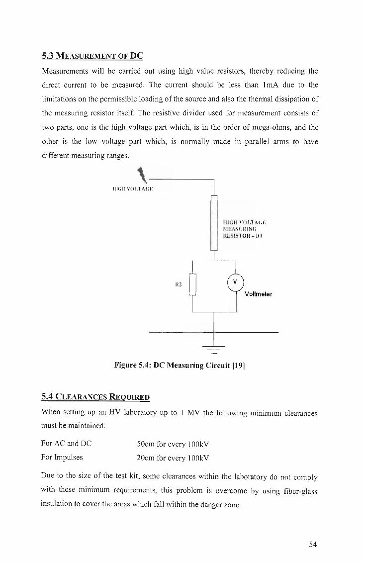
5.3 MEASUREMENT OF DC

Measurements will be carried out using high value resistors, thereby reducing the

direct current to be measured. The current should be less than lmA due to the

limitations on the permissible loading of the source and also the thermal dissipation of

the measuring resistor itself. The resistive divider used for measurement consists of

two parts, one is the high voltage part which, is in the order of mega-ohms, and the

other is the low voltage part which, is normally made in parallel arms to have

different measuring ranges.

\ -------.

IU

IIIGII VOLTAGE l\IEASUIUNG RESISTOR - RI

Voltmeter

Figure 5.4: DC Measuring Circuit [19]

5.4 CLEARANCES REQUIRED

When setting up an RV laboratory up to 1 MV the following minimum clearances

must be maintained:

For AC and DC

For Impulses

50cm for every lOOkV

20cm for every lOOkV

Due to the size of the test kit, some clearances within the laboratory do not comply

with these minimum requirements, this problem is overcome by using fiber-glass

insulation to cover the areas which fall within the danger zone.

54

5.5 EARTIDNG OF LABORATORY AND EQUIPMENT

The laboratory may only be entered once all the components that can assume high

voltages in the contact zone are earthed.

Interlocking doors ensure that once the laboratory is entered, the supply to the test kit

is immediately cut. Earthing is only allowed by a conductor that is earthed within the

test area [19].

The earthing within the laboratory is done by means of earthing rods, as well as an

automatic earthing switch. Earthing may only take place once the current source has

been switched off, and may be removed only when there is no one present in the

testing area or if the testing area is cleared once the earth has been removed.

All metallic parts of the setup which do not carry potential during normal testing has

to be earthed reliably with at least 1.5 mm2 copper conductor.

Figure 5.5: Earthing Rods

55

5.6 TEST SYSTEM SPECIFICATIONS

ACVOLTAGE

Rated Voltage 100 kV (rms)

5 kV A - Continuous Rated Output (Continuous)

7.5 kVA - Short time

Frequency 50Hz

5% approximately with respect to

Short Circuit impedance Voltage rated continuous kVA and rated

voltage.

DC VOLTAGE

No Load Rated Output, Positive Polarity 500kV

Negative Polarity 540kV

Rated Continuous Current 7.5 mA

Ripple Voltage ~ 3% at rated current and voltage

Table 5.1: Test Kit Specifications [19].

5.7 ELECTRICAL BLOCK DIAGRAM OF THE LABORATORY TEST SET-UP

Below follows a block diagram of the laboratory set-up. As can be seen an isolating

transformer is used for protection. The 220V AC supply is connected to the isolating

transformer, which in turn is connected to the high voltage test transformer. The HV

transformer is connected to the rectifier that outputs the DC voltage, This voltage is

then applied to the corona cage which is connected to earth via a measuring

impedance which is discussed in a later chapter.

High Isolating Voltage Rectifier Corona

Transformer Transformer r---- Cage

Figure 5.6: Laboratory Block Diagram

56

5.8 SUMMARY

The high voltage DC test kit at the University of Durban Westville is capable of

delivering 540 kV Negative DC and 500 kV Positive DC. It utilises a Cockcroft -

Walton rectifier circuit to generate DC from AC.

The clearances for AC and DC voltages are the same and is equal to 50 cm for every

100 kV. For impulse testing this requirement is reduced to 20 cm for every 100 kV.

Certain parts of the laboratory which, did not comply with these requirements were

modified in order to satisfy them.

The earthing system in the laboratory IS very sound. Copper braids are used

throughout the laboratory in order to ensure that all pieces of equipment which, are

not live are earthed appropriately. All metallic parts of the test set-up which do not

carry voltage during normal testing is earthed with at least 1.5 mm2 copper conductor.

Safety in the laboratory is of the utmost importance. The laboratory may only be

entered once all the components that can assume high voltages in the contact zone are

earthed. Interlocking doors ensure that if the laboratory is accidentally entered while

testing is taking place, the supply to the test kit will immediately be cut and earthing

applied.

57

CHAPTER 6

TEST PROCEDURES AND EQUIPMENT

The tests, test procedures, aims of the tests as well as the equipment used during

testing are discussed in this chapter.

6.1 TEST PROCEDURES

Three conductors were tested (l.OO-cm diameter, l.36-cm diameter, l.76-cm

diameter). These conductors were tested under the following conditions.

1. Strung up in the cage with no fan

2. Strung up in the cage with a fan blowing across (side fan) the cage

3. Strung up in the cage with a fan blowing "through" (front fan) the cage

a) b)

Figure 6.1: a) Configuration of Fan Blowing from the Side,

b) Configuration of Fan Blowing from the Front.

The coating was then applied to half of each conductor' s length and the tests were

then repeated, after waiting a day for the silicone to dry completely. Finally the entire

length of the conductors, were painted and once again the tests were repeated, again

after waiting a day for the silicone to dry. This procedure is shown in figure 6.2.

58

Figure 6.2: Test Procedures

6.2 TEST AIMs

The aims of the tests were to:

• Ascertain the effectiveness of the corona cage (Whether it could be used for

corona studies).

• Determine the effect of wind on corona performance in a corona cage.

• Determine the effect of a silicone coating on the corona performance of

conductors.

These aims were chosen in order to determine what can be done in order to mitigate

corona activity on conductors under HVDe potential.

6.3 MEASURING EQUIPMENT

In order to measure corona noise a series resistive element was required. The resistive

element has a resistance, which is equal or very close to the impedance of the co-axial

59

cable, which connects it to the measuring scope, which is approximately 50 ohms. By

using a parallel connection of resistors, of equal value, in a concentric ring the

reactive component or inductance is reduced to negligible proportions. The resistor

should be able to accommodate the corona loss current, which may flow through it.

The parallel combination was used in order to to ensure that the cable impedance is

matched so as to avoid reflections, which interfere with the measurements. The

paralleling spreads out the current and enhances the shielding effect

The total resistance of the concentric shunt is given by the following formula:

Where: R = resistance of one resistor

n = number of resistors

R Req =

n

The resistors all have the same power carrying capacity. So the current carrying

ability of each resistor can be calculated from the following:

Where: P = power rating of resistor

R = resistance

I=~

Each resistor has a value of 56 ohms and a power rating of SW. This means that the

total current carrying capacity of the shunt resistor will be approximately 3A. This is

much more than the expected corona loss current. Which, is expected to be at most in

the hundreds of micro amps range. Due to the nature of the progression of the project,

corona noise measurements were not considered part of the scope. An ammeter was

therefore used to measure the currents through a resistor to ground.

6.4 TESTS PERFORMED IN THE CAGE

After the cage was installed in the laboratory, tests were conducted, firstly to see that

the cage worked and secondly to gain some valuable corona data on the corona

performance ofHVDC lines.

Figure 6.3 shows the completed cage, with a conductor strung, ready for testing.

60

Figure 6.3: Completed Corona Cage

6.4.1 Initial Testing

The first tests to be conducted within the cage were to determine whether the cage

would be able to be used for corona testing. As stated in chapter 4, for the largest

conductor to be tested the cage diameter should be small enough to obtain corona at a

sufficiently low voltage. At the same time the air gap clearance between the cage and

the conductor should be large enough so that the breakdown voltage is higher than the

onset voltage. A margin of at least 50% between these two voltages permits studies to

be carried out at different conductor surface gradients above corona onset [4, 240].

The largest conductor available in the laboratory was a 1.76cm conductor, which

happens to be the earthwire used on the Cahora Bassa line. The conductor was strung

up and energised. Audible corona occurred at 60 kV, while visual corona started at 90

kV. This corresponds to electric field gradients of 15.34 kV/cm and 23.01 kV/cm

respectively. Now taking corona inception to be when audible corona occurred, this

would mean the inception voltage is 60 kV. This corresponds to a surface roughness

factor of 0.4, this value is similar to values obtained from independent tests [21]. The

voltage was increased and at 180 kV breakdown had not yet occurred. From this test it

was obvious that the cage would satisfy the basic design criterion.

6.4.2 Corona Measurements

As mentioned in earlier chapters, the corona performance of a line is an important

factor in its design. It is therefore clear that a better understanding of corona and its

61

associated effects, will help in the design and optimization of transmission lines.

Corona tests and measurements are two ways of gaining this understanding of corona.

The tests, which formed part of this thesis, were undertaken in an attempt to gain a

better understanding of the corona phenomenon in a corona cage.

6.4.3 Conductors Used in the Tests

The conductors used in the tests were as follows:

• 1 cm diameter

• 1.36 cm diameter

• 1.76 cm diameter

Photographs of these conductors are shown below.

Figure 6.4: Conductors Used for Testing

6.4.4 Silicone Rubber (RTy) Coating

1.00 cm diameter

A silicone Room Temperature Vulcanised (RTV) coating "Insilcote RV 2000" was

used on the conductors in order to determine the effect that it would have on the

inception gradient as well as on the corona loss measurements. The coating was

obtained from Mr. Roy Macey of Mace Technologies in Johannesburg.

This coating has been extensively used on insulators and bushings. The main reasons

for its use are as follows:

• Excellent arc resistance

• Fast recovery ofhydrophobicity after arcing

• Reduced contaminant collection

• Good adhesion to unprimed ceramic surfaces.

These factors influence the system as follows:

• Eliminates pollution flashover

• Reduces maintenance costs

• Improves system reliability.

A description of the physical properties of "Insilcote RV 2000" is shown below [18].

62

As supplied:

Appearance Sky blue liquid

Percentage Solids by weight 55%

Specific gravity at 25 deg C 1.2

Table 6.1: Physical Properties of Silicone Coating as Supplied

Figure 6.5: Insilcote and Catalyst

As cured:

Specific gravity 1.43

Dielectric strength 55 kV/mm

Dielectric constant at 50 Hz 3.0

Surface resistivity > 1 *1012 ohms

Volume resistivity > 2*10 13 ohms

Loss tangent at 50Hz 0.017

Water droplet contact angle (0.1 cc distilled water droplet) 100 degrees

Table 6.2: Physical Properties of Silicone Coating after curing

6.4.5 Fan for the Dispersal of the Space Charge

A fan was used in order to disperse the space charge and to measure the effect that the

space charge will have on the corona inception gradient as well as on the corona loss

levels. Readings were taken with the fan blowing air through the cage, and without

the fan blowing. An industrial pedestal fan was purchased from Luft Industries in

Durban. This fan was used to blow air across and through the corona cage in an effort

63

to quantify the space charge effect that may exist within the cage. The technical

specifications and diagram of the fan follows [16].

THROW FROM FAN IN METR~ "'" I

FS2S

B ~/-I

, ,

11 10 9 8 7 5 4 3 2 1 - ------ ----

a) b)

Dimension A B C D

Length mm 690 1930 360 615

Figure 6.6: a) Diagram of Fan used, b) Fan Speeds at Various Distances.

Speed setting 1 2 3

Fan speed rpm 1400 1250 1150

Volume m3/s 2.95 2.67 2.45

Noise dBA 56 49 46

Power Watts 200 140 120

Power factor 0.83 0.95 0.92

Table 6.3: Technical Specifications of the Fan [16]

64

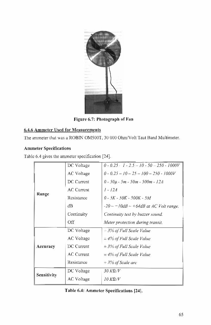
Figure 6.7: Photograph of Fan

6.4.6 Ammeter Used for Measurements

The ammeter that was a ROBIN OM500T, 30 000 OhmNolt Taut Band Multimeter.

Ammeter Specifications

Table 6.4 gives the ammeter specification [24].

DC Voltage o - 0.25 - 1 - 2.5 - 10 - 50 - 250 - 1000 V

AC Voltage 0- 0.25 -10 - 25 -100 - 250 -1000V

DC Current 0- 50IL - 5m - 50m - 500m - 12A

AC Current 1-12A Range

Resistance 0- 5K - 50K - 500K - 5M

dB -20 - + 1 OdB - +64dB at AC Volt range.

Continuity Continuity test by buzzer sound.

Off Meter protection during transit.

DC Voltage ± 3% of Full Scale Value

AC Voltage ± 4% of Full Scale Value

Accuracy DC Current ± 3% of Full Scale Value

AC Current ± 4% of Full Scale Value

Resistance ± 3% of Scale arc

DC Voltage 30 KO / V Sensitivity

AC Voltage 10 KO / V

Table 6.4: Ammeter Specifications [24].

65

6.5 SUMMARY

Initial testing of the cage proved successful. The largest conductor in the laboratory

was a 1.76 cm diameter conductor and this conductor when tested in the cage showed

that the 50% criterion between onset voltage and breakdown voltage was adhered to.

Three conductors were available for testing, they were all stranded conductors with

the following diameters, 1.00 cm, 1.36 cm, 1.76 cm.

The silicone rubber used in the testing was obtained from Mace Technologies in

Midrand, Johannesburg. The silicone has the following properties

•

•

•

•

Excellent arc resistance

Fast recovery ofhydrophobicity after arcing

Reduced contaminant collection

Good adhesion to unprimed ceramic surfaces.

A large fan was purchased. This was done so that the effects of wind on the corona

phenomenon may be studied in the cage.

66

CHAPTER 7

TEST RESULTS

In this chapter the test results are presented and analyzed. These results mainly deal

with the results of tests done to determine the effect of the silicone coating on the

corona performance of several conductors.

7.1 TEST RESULTS

In this section, all results of tests done with no fan present will be represented

graphically in red, while the results of tests done with the fan blowing through the

side of the cage will be in blue and the results obtained with the fan blowing through

the front of the cage is shown in green.

7.1.1 Effect of Wind on Uncoated Conductors

The testing of all the conductors was done under the following conditions:

• Laboratory air-conditioning off

• "Clean" surface condition

Point one above is important as some fluctuations in measurements were noticed

when the laboratory air-conditioning was on and when it was off. These first tests

dealt with the effect of wind on the corona currents generated. The conductors were

strung up and tested without any silicone coating. Corona current was measured

without any simulated wind, then with a side wind and finally with a front wind. The

results for the three conductors are now shown.

7.1.1.1 Results of 1.00-centimeter diameter conductor

The results of this set of tests seem to indicate that corona current is generally not

increased for the I.OO-cm diameter conductor, with wind blowing over it. Wind

blowing from the side of the cage has a greater impact on current increase than wind

blowing through the front of the cage. Wind blowing from the front of the cage

actually seems to decrease the measured corona current. Based on these results it is

still not certain whether the effect of wind on this conductor in a small corona cage is

significant.

67

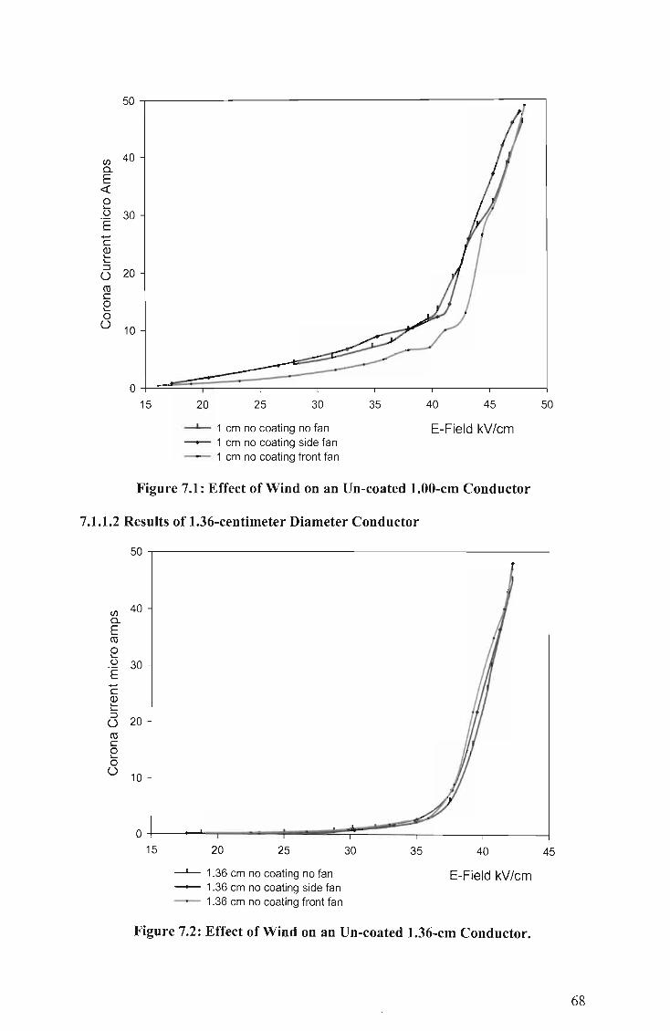
50~------------------------------------------~~

Cl) 40 c.. E <t: 0 ... u 30 ·E -c (]) ... ... ::I

20 ()

CO c 0 ... 0 ()

10

15 20 25 30 35 40 45 50

--I- 1 cm no coating no fan E-Field kVfcm - 1 cm no coating side fan - 1 cm no coating front fan

Figure 7.1: Effect of Wind on an Un-coated LOO-cm Conductor

7.1.1.2 Results of 1.36-centimeter Diameter Conductor

Cl)

c.. E co 0 ... . ~ E -c (]) ... ... ::I ()

co c e 0 ()

50.--------------------------------------------------

40

30

20

10

15 20 25

--I- 1.36 cm no coating no fan - 1.36 cm no coating side fan -- 1.36 cm no coating front fan

30 35 40

E-Field kV fcm

Figure 7.2: Effect of Wind on an Un-coated 1.36-cm Conductor.

45

68

The results shown in figure 7.2 indicate that the effect of wind is not a major

contributor to corona current increase. Based on these results it is also not clear what

effect wind has on a stranded, clean un-coated conductor. Generally it seems as

though the corona current measured without the fan blowing from the front or the side

is lower, but only marginally. This result is not conclusive on its own.


Cl)

Cl. E « 0 ~

u E -c ID ~ ~

:::J U co c 0 ~

0 U

50

40

30

20

10

5 10 15 20

---I- 1.76 cm no coating no fan - 1.76 cm no coating side fan - 1.76 cm no coating front fan

25 30

E-Field kV/cm

Figure 7.3: Effect of Wind on an Un-coated 1.76-cm Conductor.

35

Figure 7.3, is also not conclusive with regards to the effect of wind on the corona

current generated. From the results obtained it seems as though the effects of wind in

a corona cage on a clean, stranded, un-coated conductor are minimal. For conductor

surface gradients in excess of 25kV fcm, the corona currents generated with the fan

blowing is once again marginally higher than those recorded without the fan blowing.

7.1.1.4 Discussion of the Effects of Wind on Un-coated Conductors in the Corona

Cage

Figures 7.1, 7.2 and 7.3 indicate that the effect of wind on a clean, stranded, uncoated

conductor in a corona cage is minimal. These results were quite surprising since it was

expected that the effect of wind blowing over the conductor would have had a greater

69

effect on the corona current, than what was measured. However, previous work done

by Khalifa and Morris [1] showed that wind had little effect on corona losses on

monopolar lines in a one conductor to ground plane, configuration, which is basically

the similar to the cage set-up. Further testing is required with a more powerful fan. It

is also recommended that similar tests be performed with the surface condition of the

conductors being changed, i.e. decreasing the roughness factor.

7.1.2 Effect of Wind on Half Coated Conductors

The conditions under which these conductors were tested were the same as the

conditions described in section 7.1.1 These tests were carried out a day after the tests

discussed in section 7.1.1 The results of these tests are given below.

Figure 7.4: Half-coated conductors'


50

(J)

0. E 40 « 0 ~

u E 30 -r:::: ~ ~

::3 U

20 tU r:::: e 0 u

10

15 20 25 30 35

--I- 1 cm half coated no fan - 1 cm half coated side fan - 1 cm half coated front fan

40

E-Field kV/cm

45

Figure 7.5: Effect of Wind on a Half Coated 1.00 cm Diameter Conductor

70

These results shown in figure 7.5, once again seems to indicate that the effect of wind

on this type of conductor in a cage is minimal, not withstanding the fact that the

conductor is now half-coated with silicone. In fact, for a certain interval of electric

field strength, the corona current due to the fan not being present is actually higher

than when the fan is blowing from the front or from the side.


The results shown in figure 7.6 are interesting due to the fact that the corona current

produced with the fan blowing from the front of the cage is higher than when it blows

from the side or when it is not blowing at all. Similarly the corona current produced

when the fan is blowing from the side position is generally higher than the current

produced when the fan is not blowing at all. This result would seem to indicate that

the effect of wind on this specific conductor is such that it increases the corona current

produced. The fan blowing from the front has a greater impact of corona current

increase than the fan blowing from the side, which in turn produces more corona

current than when it is not blowing at all.

50

IJ) a. E 40 « 0 L.. ()

'E 30 .-

c ID L.. L.. ::J U ro 20 c 0 L..

0 U

10

O+-~~~~-,--------~----------~---------15 20 25 30 35

--J- 1.36cm half coated no fan E-field kV/cm - 1.36 cm half coated side fan - 1 .36cm half coated front fan


71


50

Cl)

c. E 40 « 0 ...... u ·E 30 -c Q) ...... ...... :::J U co 20 c 0 ...... 0 ()

10

12 14 16 18 20 22 24 26 28 30

---L...- 1.76cm halfcoated no fan E-Field kV/cm - 1.76cm half coated side fan - 1.76cm half coated front fan


The results in figure 7.7 are similar to the results shown in figure 7.3. However this

time the difference is more marked. Corona currents produced while the fan was

blowing are generally the same whether the fan was placed in front of the cage or at

the side of the cage, while corona currents measured without the fan are generally

lower. This would seem to indicate that wind blowing over this conductor has more of

an effect when it is half coated than when it is not coated at all.

7.1.2.4 Discussion of the Effects of Wind on Half Coated Conductors in the

Corona Cage

The results of the effects of wind on half silicone-coated conductors differs markedly

from the results obtained in the precious section. One of the main differences is that

for similar electric field levels the corona current measured for the half-coated

conductors are higher than that measured for the un-coated conductors. For the 1.00-

cm diameter conductor the results are similar to the results for all the conductors in

the preceding section, however for the larger conductors we notice a difference.

For the 1.36-cm diameter conductor, the corona currents produced when the fan blew

from the front of the cage is higher than when it blew from the side or when it was

72

switched off. The lowest average corona currents were measured when the fan was off

and the highest when the fan was blowing from the front. This indicates that wind

blowing over this specific conductor when it is half coated with silicone, increases the

corona current produced.

The 1.76-cm conductor is very different to the previous two conductors tested. The

results obtained for the corona current when the fan was blowing from the side and

from the front are almost identical, while the current measured when the fan was

switched off is much less.

The results from the three conductors indicate that the effect of wind on the half

silicone-coated conductors increases as the conductor diameter increases. There is

also not much of a difference in the effect produced by wind from the side or the front

of the cage.

7.1.3 The Effect of Wind on Fully Coated Conductors

Once again the test conditions for testing fully coated conductors follows the

procedures described in chapter 6. The conditions under which testing took place are

also the same as in sections 7.1 .1 and 7.1.2. These tests took place a day after the tests

described in section 7.1.2 and two days after those described in section 7.1 .1.

Figure 7.8: Fully coated conductors'


The results shown in figure 7.9 below are similar to the results obtained in figure 7.5

where we had a half silicone-coated conductor. Generally the effect of wind seems not

to play a major role in the corona current produced by this specific conductor even

with it being fully silicone-coated. It would be safe to say that this conductors '

performance is not affected by wind to such an extent where the corona current

produced rises markedly.

73

50

Cl) Q.

E 40 <X: 0 '-()

E 30 -c Q) '-'-::J ()

cu 20 c 0 '-0 ()

10

15 20 25

-'- 1 cm full coated no fan - 1 cm full coating side fan - 1 cm full coating front fan

30 35

E-Field kV/cm

40

Figure 7.9: Effect of Wind on a Fully Coated LOO-cm Diameter Conductor


50

Cl)

a. E 40 « 0 '-()

E 30 -c Q) .... .... ::J ()

cu 20 c 0 .... 0 0

10

O+---~--~.----.----.----.----.----.----.----.--~

14 16 18 20 22 24 26 28 30 32 34

----L- 1.36 cm full coating no fan E-Field kV/cm - 1.36 cm full coating side fan -- 1.36 cm full coating front fan

Figure 7.10: Effect of Wind on a Fully Coated 1.36-cm Diameter Conductor

74

The results obtained for the fully coated 1.36-cm fully silicone-coated conductor is

very similar to the results obtained for the half silicone-coated 1.36-cm conductor.

The main difference however is the fact that the corona current has been increased.

Under the half silicone-coated condition a surface gradient of 25 kV/cm produced

currents ranging from 12 to 14 !lA. Under the fully silicone-coated condition 25

kV/cm corresponds to currents of between 18 and 25 !lA. This will be further

discussed in section 7.2.


As with the results shown in figure 7.10, the results shown in figure 7.11 are similar to

the results for the conductor when it is half coated, as shown in figure 7.7. Once again

the main difference is the increase in corona current measured from the half coated to

the fully coated version. For example at 20 kV/cm the half silicone-coated conductor

gives values of between 8 and 13 !lA. On the other hand the fully silicone-coated

conductor gives values of between 12 and 18 !lA.

(J) a. E <{ 0 .... u ·E -c (l) .... .... ::l ()

ro c 0 .... 0 ()

50

40

30

20

10

O+-~--'-----.-----~-----r----~----~----~----~

14 16 18 20 22

~ 1.76 cm fully coated no fan - 1.76 cm fully coated side fan - 1.76 cm fully coated front fan

24 26 28 30

E-Field kV/cm

Figure 7.11: Effect of Wind on a Fully Coated 1.76-cm Diameter Conductor

75

7.1.3.4 Discussion of the Effects of Wind on Fully Coated Conductors in the

Corona Cage

These results tend to indicate that the effect of wind IS more pronounced on

conductors that are fully silicone-coated.

For the 1.00-cm conductor, the results seem to indicate that although the conductor is

fully coated, there is not much of a difference in corona current when the fan is

positioned from the side, from the front or not on at all.

The 1.36-cm conductor has a major difference between corona loss when the fan is off

and when it is on. The lowest currents were measured when the fan was off and the

highest when the fan was in front of the cage.

The results for the 1.76-cm conductor are similar to those of the 1.36-cm conductor

except the differences between the currents measured with the fan from the side and

from the front are not as big as for the 1.36-cm conductor.

7.2 FURTHER ANALYSIS OF TEST RESULTS

In this section, all results of tests done with no coating present on the conductor will

be represented graphically in red, while the results of tests done with the conductor

half silicone-coated will be in blue and the results obtained with the conductor fully

silicone-coated is shown in green.

These graphs were produced after analysis of the results obtained from the first set of

tests performed in the cage. This was done in an effort to determine the effect of the

coating on the corona losses incurred by the conductors.

7.2.1 Effect of Coating with No Fan Present

The data from the tests performed without any wind was used to draw these graphs.

The results used in the graphs, obtained for un-coated conductors were obtained a day

before the results for the half silicone-coated conductors which was in turn obtained a

day before the results for the fully silicone-coated conductors.


Figure 7.12 indicates that the corona current is dramatically increased when the

conductor is coated with silicone. The fully silicone-coated conductor has the highest

measured current of the three. With the uncoated conductor having the lowest

measured current. At a surface gradient of 30 kV/cm the uncoated conductor produces

76

a current of about 5 !lA, while the half-coated conductor produces a corona current of

14 !lA and the fully coated conductor produces a current of about 20 !lA.

50

en a. E 40 4: Q I.-()

·E - 30 c Q) I.-I.-

:J U

20 co c Q l.-

Q U

10

15 20 25 30 35 40 45 50

-'- 1.00 cm no fan no coating E-Field kV/cm -- 1.00 cm no fan half coated - 1.00 cm no fan full coating

Figure 7.12: Effect of the Coating on a Wind Free LOO-cm Diameter Conductor


These results are similar to the results obtained for the 1.00-cm conductor. At 30

kV/cm, the un-coated conductor produces a current of about 1 !lA, while the half

coated conductor, produces a current of 28 !lA and the fully coated conductor,

produces a current of 41 !lA. The results of the un-coated conductor is not accurately

with respect to the results obtained for the half coated and fully coated conductors, as

the corona current was measured for the 1.00-cm conductor, by increasing the voltage

from zero while the other measurements were made by decreasing the voltage from

the maximum possible, for the specific conductor in the cage and the scale on the

ammeter.

77

50

en 0. E 40 <t: 0 "-()

E ...... 30 c (l) "-"-::l 0

20 ro c 0 "-0 0

10

15 20 25 30 35 40 45

--L- 1.36 cm no fan no coating E-Field kV/cm - 1.36 cm no fan half coating - 1.36 cm no fan fully coated

Figure 7.13: Effect ofthe Coating on a Wind Free 1.36-cm Diameter Conductor


en 0. E <t: 0 "-()

·E ...... c (l) "-"-::l U ro c 0 "-0 0

50

40

30

20

10

O+---------,-----~--.---------r_------_.--------~

10 15 20

--L- 1.76 cm No Fan no coating - 1.76 cm No Fan half coated -- 1.76 cm no fan fully coated

25 30

E-Field kV/cm

35

Figure 7.14: Effect of the Coating on a Wind Free 1.76-cm Diameter Conductor

78

Once again these results are similar to the results obtained for the 1.00-cm conductor

as well as those obtained for the 1.36-cm conductor. This time when the conductors

experienced a surface gradient of 30 kV/cm, the half coated conductor produced a

corona current of about 30 /-lA, while the half-coated conductor produced a current of

over 50 /-lA and the fully-coated conductor produced a current which was above the

half-coated conductor current. The current could not be measured by the ammeter as it

could only measure up to 50 /-lA. The assumption that was made that the fully coated

conductor would produce a higher corona current than the half coated conductor is

valid since this was the trend shown by the previous two examples.

7.2.1.4 Discussion ofthe Coating Effects with No Fan Present

The results that were shown in the three graphs above are quite surprising. It was

expected that the application of the silicone coating would decrease the corona

currents measured since it would decrease the surface gradient experienced on the

conductors' surface. See appendix D.

7.2.2 Effect of Coating with a Side Fan Present

As was stated before these results were obtained from the tests done previously, the

data was manipulated and represented graphically. The results below show the effects

of the silicone coating on the conductors when the fan was blowing from the side

position.


The results of the 1.00 cm diameter conductor with the fan blowing from the side, are

shown in figure 7.15.

These results are similar to those obtained when the fan was off, however there does

not seem to be major difference for the corona currents measured for the conductor,

when the fan is blowing from the side or when it was not blowing at all.

79

50

en c.. E 40 « 0 .... C,.)

'E 30 .-

c Q) .... .... ::J ()

20 CO c e 0 ()

10

O+-~~-'-----'------.-----'------'------r---~ 15 20 25 30 35 40 45 50

---L.- 1.00 cm side fan no coating E-Field kV/cm ---L.- 1.00 cm side fan half coating ---L.- 1.00 cm side fan full coating

Figure 7.15: Effect of the Coating on Side Wind Blown 1.00-cm Diameter Conductor


50

en c.. E 40 « 0 .... C,.)

'E 30 .-

c Q) .... .... ::J 0

20 co c 0 .... 0 ()

10

15 20 25 30 35 40 45

---L.- 1.36 cm Side Fan no coating E-Field kV/cm ---L.- 1.36 cm Side Fan half coated ---L.- 1.36 cm Side Fan fully coated

Figure 7.16: Effect of the Coating on Side Wind Blown 1.36-cm Diameter Conductor

80

The results are shown in figure 7.16. Once again these results are similar to those

obtained when the fan was not present. As is the case with the previous graphs, the

coated conductor has the highest measured corona current, followed by the half-

coated conductor.


50

en a. E 40 <t: 0 ..... u 'E - 30 c Q) ..... ..... ::J ()

20 ro c e 0 ()

10

5 10 15 20 25 30 35

--'-- 1.76 cm Side Fan no coating E-Field kV/cm --'-- 1.76 cm Side Fan Half Coating --'-- 1.76 cm Side Fan Full Coating

Figure 7.17: Effect of the Coating on Side Wind Blown 1.00-cm Diameter

Conductor

Again we see that the results are similar to the results obtained for the same conductor

without the fan present. We notice that this time the highest currents are recorded for

the fully coated conductor as well as for the half-coated conductor while the lowest

currents are measured for the un-coated conductors.

7.2.2.4 Discussion of the Coating Effects with a Side Fan Blowing

As with the results obtained for the effects of the coating with no fan present, we

notice that the coating increases the corona currents measured. Once again the larger

diameter conductors produce higher corona currents at the same applied field when

compared to the smaller diameter conductor. This is due to the higher applied voltage

81

required to obtain the same electric field strength on a large conductor in comparison

to the voltage required to obtain that specific field strength on a smaller conductor.

7.2.3 Effect of Coating with a Front Fan Present


50

Cl)

D-E 40

c::x: 0 '-()

'E ..... 30 c Q.) '-'-::::l U

20 cu c 0 '-0 U

10

15 20 25 30 35 40 45 50

---L.- 1.00 cm front fan no coating E-field kV fem --'-- 1.00 cm front fan half coated ---L.- 1.00 cm front fan full coating

Figure 7.18: Effect of the Coating on a Front Wind Blown 1.00-cm Diameter

Conductor

As can be seen from the figure above these results are once again similar to the

previous results obtained for this specific conductor. Since the effect of wind was

minimal on this specific conductor the results being similar are what was expected.


Again the results are similar to previous results taken. Once again the fully coated

conductor has the highest corona currents measured with the half-coated conductor

having the second highest measured corona current. This result follows the trend of

the 1.00 cm diameter conductor. This was expected since it was earlier shown that the

effect of wind on the conductors was minimal.

82

50

Cl)

0. E 40 « 0 ~

u 'E - 30 c Q) ~ ~

::::l ()

20 co c 0 ~

0 ()

10

15 20 25 30

----L.- 1.36 cm Front fan no coating ----L.- 1.36 cm Front fan half coated ----L.- 1.36 cm Front fan Fully coated

35 40

E-field kV/cm

45


Conductor


Finally we see that the results obtained for this conductor once again follows the trend

set out by the other two conductors to be tested. This is shown in figure 7.20.

However this time the differences in the corona currents measured from when the fan

was blowing to when it was off is not as marked as in previous cases. Also the results

for the half coated conductor and for the fully coated conductor are closer together.

This could imply that the effect of the coating is not that much between a fully coated

conductor and a half coated conductor for this specific conductor.

83

50

C/l Cl. E 40 CO 0 ~

()

'E 30 c

Q) ~ ~

:l 0 20 CO c 0 ~

0 0

10

o +-----.----.-----.-----,-----r----,-----.----,,---~ 16 18 20 22 24 26 28 30 32 34

E-Field kV/cm

--'-- 1.76 cm Front Fan no coating --'-- 1.76 cm Front Fan Half coated -I-- 1.76 cm Front Fan fully coated


conductor

7.2.3.4 Discussion of the Coating Effects with a Front Fan Blowing

As with the results obtained when the fan was off and when the fan was positioned to

the side of the cage, the coating increases the corona current measured when the fan

blows from the front of the cage. These results are similar to the results obtained for

the other two conditions.

7.3 Analysis of the Effect of the Silicone Coating

The effect of the silicone coating on corona currents and corona losses measured was

unexpected. It was hypothesized that the use of the silicone coating would decrease

the corona currents measured and therefore decrease corona losses incurred. This,

however, was not the case.

In an attempt to explain this phenomenon of increased corona activity when the

coating was applied, a time domain analysis of the current pulses was done. This

analysis was carried out using a 1.36 cm diameter conductor, initially the conductor

84

was tested without a coating present, then with half of it coated and finally it was

tested after being fully coated. Thereafter the coating was stripped off the conductor

and the tests repeated after the conductor was sanded down with sandpaper.

7.3.1 Analysis of the Uncoated conductor

As can be seen in figure 7.21 , the voltage pulses are fairly wide spread from each

other. The current pulses are in phase with the voltage pulses and flow through a fifty

ohm resistor. The 0.5 V Idivision of the voltage pulses thus corresponds to a 10

mA/division for the current pulses. From this point forward the voltage per division

will be divided by the resistor value to get the current value per division. The supply

voltage was 112.5 kV, which corresponds to a surface gradient of35 .18 kV/cm.

Z88Z,,8CJ...-06 16 :31: 58%'11 UJl0k Nor"a 1 Sto ed 1343 .,. SftS/S Z88t1:r.M.ioo

< /tell",.10k » : · . . . . . ......... : .... . ... - : ... ... . . . : . ... .. . . ... ...... ; ...... . . . : ......... : · .. . . · . . ... · .. .. . ........ . : ......... : .. .. .. .. . : . . .... .. . - .. . . . .. : ... ... .. : ..... . . .. : · .. .. . · . . .. . .. . . .

. . · . . · . . ..... . .. . .... . ......................... · . . · .. .. · . . .. · . . " .. . . ... . . : .. ....... : . . .. . .... : .. .. . . . . . .. .. .. .. : .... . . .. .. : ....... . . ... .. -....... . .. . : . ... . .. . . · . . . . · .. . . .. ....... : ..... .... : . . .. . .. . . : .. . ... . . . ........ : .. .. . ... . : ....... .. .... .. . .. . ... .. . .. : .. · .. . . · . - . . · . . . .

.. . . . . ... ' : .. .. ... . . : . ... .. .. . : .. . ............... : . ... . .... : . ....... . : ..... .... ...... ... : · .. . . . . .. . . . . .. . .. .

....... • • : ...•....• : . .• . .. ....•.. • •• • • • ••• . ••• : • • .• • ••• • ! • ••• • •• • • : • • •. . . • ••• . •••• .. . : . .... . . . • . . ... . . . .. . . .. . . . . .... : . .. . . .... : . . . . ..... : .. .......... .. .. .. : ... . .... . .. . . . . . . . . . . . . . ...... . .. : .... .. ... : ............. ..... ..... .. ... ; . ... ... .. ; . .. ... ... : .. . ...... . .. .. ... . : .. . ... . . . . ... . . . . .. . .. . . . . .. ...... .. : ......... ; .......... . ... .. ... . .... . . .. : . .. . . ... . : ...... ... : . .... . . .. .. .... . . . : ........ .

" ... . .. . .. . .. . ...... : ..... .. .. : ... .... .. ........ . ; . .. ..... . . : .... .. .. . : .. ..... .. : . .. ....... .. . .. .. . : . . ...... . . . .. . . . ;: :: : : :

Edge CH1 S Auto 8.eee U

Figure 7.21: Time domain analysis of Un coated conductor corona current pulses

7.3.2 Analysis ofthe Half coated conductor

The results for the half coated conductor is shown in figure 7.22 as can be seen, the

current pulses are much more frequent than for the uncoated conductor. This could be

ascribed to the fact that the capacitance of the cage to conductor configuration has

been changed with the introduction of the silicone coating. This will be discussed later

in this chapter. The applied voltage was once again 112.5 kV, which corresponded to

a surface gradient of35.18 kV/cm.

85

Z00Z,0')/e6 16: 06: 58Z1~!I====~~====3DI010k St~ ed 185'3 T

Nornal sns,s Z0~:IOIolW

... (l.1 .... Jl0'-: )')

.. . . . ... . ~ .. .. ..... ~ ......... ~ ... .. ..... . ... .. ~ .... . . . .... . ...... ~ ......... ~ . ........ .

. . . . · . . . . . . .. ..... .. .. . ..... ... ~ .. -.... . . ~ ... .... . . ~ . . . . . . . .. . .. .. ... . ~ . . . . . . . .. . .. ..... . . ... . ... . · . . . . . . .. .. .. ...... . ........ ~ .... .. ... ~ ..... ..... ~ .... -. . .. . .... .. ... ~ '. . . . . . . .. .. ... ... . . .. . . ... . · .. .... .. ; . . . . . . . .. . .... .... [ ..... .... [ ...... ... ~ . . . . . . . . . . ........ ~ . . . . . . . .. . . ... . ... ; .. . ..... .

Edge CH1 S Auto 0 . 000 U

Figure 7.22: Time domain analysis of Half coated conductor corona current

pulses

7.3.3 Analysis of the Fully coated conductor

The trend displayed in figure 7.22 is repeated in figure 7.23. A note should be made

that in this figure the current division is 20 mA/division. Once again the current pulses

have increased in frequency. As before this can be ascribed to the increase in the

capacitance of the cage to conductor configuration. This time the applied voltage was

116.8 kV this corresponds to a surface gradient of36.52 kV/cm.

Z00Z,0'3,e6 15: 1'3: 15 z1 [] --------------------1 IOk Nornal St~ eel 4365 T SIIS/S ze""sAw

· ; < < l'1G.i nl 1 Ll k > > : _ · ... . . . . .. . .. . . . ... . : . . . . . .... : ...... . .. : . . . .. . . . . : ...... . .. : ....... . . : ... ...... : ..... . . : . ..... . · .... . . : :::: :: ... ... .. . : . ..... .. . : ..... .... : . ... ... . . : . .... . ... : ... .... .. : ...... ... :, ..... . · .. . . . · . .. . · . . . . . . .. . ...... : . . . .. ... . : ... .... .. : ......... : ... . .. . .. : .. .. ..... : .. ... . ... : ..... . · . .. . · . .. . · . .. .

· . . . .. . · . . . . . . · . . . . . . . ... . ... : . . .. . .. .. : ......... : . .. . .... . : . . . . . . . . . : ... .. .... ; .. . .... : . ... . .... : ... . .. , .. : : : : : : : : .. . .. . .... .. .. . . .. ~ - . -. - .- .. ~- ..... .. . ~ .... ..... ~ .. . . .. ... ~ ....... .. ; .... .. . ~ .... .. ... ~ ........ .

......... ......... : . ... .. . . ': . .. .. . ... : ....... ': . ........ : . ........ : .... .. . : ......... :. : :. : ; :

.. . . . .... ~ ... . .... . ~ .. ....... ~ .. ...... . ~ ........ ~ ......... ~ . . .. . . . .. : . . ...... . ~ . . . ...... : .. .

..... .... : .. . ..... . : ...... ... : .. ..... . . . . . : . ... . . . .. : . ..... . .. : ..... ... . : ... .. .... : .... .... . · . . , . . .. . · . . . . . . · . . . . .

.. . ~--~----~--~. ~.~~ .. ~.:.~ .. ~ .. ~ .. ~ .. ~.~ ... ~ .. ~ .. ~.

· . . . . . . .. . ... ..... : . .. . . . ... ~ . . . . . . . . . . .. ...... : . . .. ... . . ~ . ... .... . ~ ......... ~ . . . . . . . .. . ....... .

::::: :::: .: :::::::!::::::::: j:: :::::::!: ::: :::: :~:. : : ::::::1:::: ::: :: j: ::::::: :1 ::::: :::: :: ::::::: : : ; : : : :

Edge CH1 S AU1:o 0.000 U

Figure 7.23: Time domain analysis of Fully coated conductor corona current

pulses

86

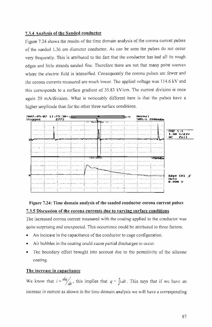
7.3.4 Analysis of the Sanded conductor

Figure 7.24 shows the results of the time domain analysis of the corona current pulses

of the sanded 1.36 cm diameter conductor. As can be seen the pulses do not occur

very frequently. This is attributed to the fact that the conductor has had all its rough

edges and little strands sanded fine. Therefore there are not that many point sources

where the electric field is intensified. Consequently the corona pulses are fewer and

the corona currents measured are much lower. The applied voltage was 114.6 kV and

this corresponds to a surface gradient of 35.83 kV/cm. The current division is once

again 20 mAldivision. What is noticeably different here is that the pulses have a

higher amplitude than for the other three surface conditions.

Z00Z,...0'J/07 11 :Z'J :302 '0 - I Sto ed Z773

· . « Mo.i k » · . · . . .. ...... .. . . ... -. . . ; ... .. .... : . . ....... ........ . · .

. . _ .... .. . . . _ . . . .. ... : . . _., .... . ~ --:' ....... -- ........ . . ... -,-

. ... ... .... .... ..... . : . ........ : ......... : .. .... .. . · . . · . . · . .

. . . . . . . .. . ..... ... i . . . . . . . .. .. _._.d • . .. ; . • . • • • • •• • • • . .. _. . .••... . .. . . ...... . ~ - • •••• • • • : •• • •••• • • . . . . . _ .. . -.-.. . . -.. . . -. :' ., . ... ~ ..... , .. -. " " :' . _ ... .... .... -.. . .... .. .. ... .... ..... : . .. --... . . . .. .. . _.

.: : ... _-- . ' . " ' .... . ... . :." ... '.- . . . . . ..... . . : . .... . .. . · . · .

. . .. .... . ; ..... . ... : .. . ... .. . : . .. .. .. . . : ...... . . . · . .

Edge CH1 S Auto 9.000 V

Figure 7.24: Time domain analysis of the sanded conductor corona current pulses

7.3.5 Discussion of the corona currents due to varying surface conditions

The increased corona current measured with the coating applied to the conductor was

quite surprising and unexpected. This occurrence could be attributed to three factors.

• An increase in the capacitance of the conductor to cage configuration.

• Air bubbles in the coating could cause partial discharges to occur.

• The boundary effect brought into account due to the permitivity of the silicone

coating.

The increase in capacitance

We know that i = d%t' this implies that q = fi.dt. This says that if we have an

increase in current as shown in the time domain analysis we will have a corresponding

87

increase in the charge q. Now as was shown for the same applied voltage, the

currents measured with the coating applied was higher than those measured without

' the coating. The formula, which relates the charge to the applied voltage, is as

follows: q = CV . Where C is the capacitance. Now if the voltage remains constant

and the charge measured increases this implies that the capacitance has increased, as

shown in the following formula, C =!l. Capacitance is defined as the ratio of the V

charge on one of its conductors to the potential difference between the conductors. A

capacitor is defined as an electrical device, which consists of two conductors

separated by a dielectric medium and is used for storing electrostatic energy [28]. The

definition of a capacitor gives an indication of what could be increasing the

capacitance of the cage to conductor configuration. The relative dielectric strength of

air is taken as 1. The dielectric strength of the coating is 2.4 [18] relative to air. All

calculations will employ the use ofthe relative dielectric strengths of the materials.

For the conductor to cage configuration shown in figure 7.25 the capacitance in

Farads/meter is given by the following formula: C 27r&2 where Ez = relative

= In(~) '

dielectric strength of air, c = radius of the cage, a = radius of the conductor.

Figure 7.25: Cage and conductor configuration

The electric circuit diagram of figure 7.25 is as follows:

c v R

Figure 7.26: Electric diagram of the conductor and cage configuration

88

Where, V is the applied voltage, C is the capacitance of the conductor to cage

configuration and R is the measuring resistance.

Now with a coating applied to the conductor the configuration changes as follows:

Figure 7.27: Corona cage with a coated conductor

As shown in figure 7.27 the coating has changed the conductor to cage configuration.

There will now be an extra capacitance between the conductor and the coating. The

capacitance in Farads/meter is as follows, C 27r&J h . hI' J = ( b)' ere E I IS t e re ahve

In -a

dielectric strength of the coating, b = radius of the coating and a = radius of the

conductor. Furthermore the capacitance in Farads/meter of the cage to coating will

now be as follows, C2 = 27r.(:2), where E2 is the relative dielectric strength of air, c = In -

b

radius of the cage and b = radius of the coating.

v

Figure 7.28: Electric diagram of the conductor, coating and cage configuration

In the figure above, V = applied voltage, Cl = capacitance between the conductor and

the coating, C2 = the capacitance between the cage and the conductor and R =

measuring resistance.

89

Without the coating the capacitance of the conductor to cage configuration for a 1.36

cm diameter conductor is

C = (21Z'.1) F/m = 1.33595 F/m. ln~

0.68

Now with the coating having a thickness of 0.75 mm the capacitance of the coating

and conductor configuration is as follows,

Cl = 21Z'.(2.4) F/m = 6.844*103 F/m. In(0.6815)

0.68

This implies that the charge which gets produced between the coating and the

conductor is much higher than what gets produced in air, since the capacitance in the

coating is much higher than the capacitance of free air.

The coating to cage capacitance is as follows,

c, ~ (".1 ) F/m ~ 1.33658F/m. in 75

0.6815

Once again we see that the capacitance of the coated conductor to cage configuration

is higher than that of the uncoated conductor to the cage. So more charge will get

produced in this region than what will be produced in air if there was no coating on

the conductor.

Both the coating to conductor region as well as the cage to coating region now has a

higher capacitance value than the single cage to conductor region. This implies that

together both regions will produce more charge than what was produced by the single

region. Consequently, more current will be produced.

We can now calculate the total capacitance of the two regions. From figure 7.28 we

see that Cl and C2 are in series therefore we add them as follows,

1 Ct =-2--

I _I I CIl

--1--1--1-=1.33632 F/m.

----+---6.844 * 103 1.33658

90

This value is 370 IlF/m higher than what was calculated for the single regIOn

capacitance (i.e., the capacitance of the uncoated conductor to the cage).

Increase in current due to partial discharges

The increased current could also be attributed to microscopic air particles, which

could have existed in the silicone rubber coating. This can be modeled using a field

simulation software package [23].

The figure below shows that these microscopic air particles would cause local electric

field intensification within the coating. Once again QUICKFIELD was used for the

field modeling.

1 .0010 1.3900

1 .0007 1 .3182

1 .0004 1.2464

1.0001 1.1746

0 .9998 1.1028

0 .9995 1 .0310

0.9992 0 .9592

0 .9989 0 .8874

0 .9986 0 .8156

0 .9983 0 .7438

0 .9980 0 .6720

Figure 7.29: Uniform and non - uniform field distribution

The first block above corresponds to a cross sectional area of the silicone rubber used

on the conductors. The legend on the left is associated with this block. As can be seen

this simulation was carried out without any air particles present in the coating. The

uniform field obtained due to this is as expected, uniform. The field has a value of

about 1.0 * 107 Vim.

91

The second block represents the coating with air particles present. The area inside

these particles has a relative permittivity of 1, while the rest of the area in the block

has permittivity of 2.4. As a result of these air particle, we can see an intensification

of the electric field within the silicone. The eletric field is now non-uniform. With the

field strength across the air particles being the highest. This field strength can be

quantified by using the right hand side legend. The peak value of the field is l.39 *107

Vim. This is 39% higher than the value of the field measured without air particles

present. If this field value is high enough, we may have partial discharges occuring

across the air particles.

Increase in E-Field in air due to boundary effects

From electromagnetic field theory we know that the normal component of electric

flux density across a charge - free boundary, must be continous. This implies that the

normal component of the flux density at the surface of the coating has to be equal to

the normal component of the flux density of the air adjacent to the coating. This leads

to the following equation:

Where: Drl = flux density in region 1 (the coating) at radius r.

Dr2 = flux density in region 2 (air) at radius r.

Since D = 8E, this implies that:

at the boundary r. Where: 81 and 82 are the permitivities of the coating and air

respectively.

El and E2 are the electric field gradients in the coating

and air respectively.

The coating has a permitivity 2.4 times that of air. This means that the electric field

gradient in the air is 2.4 times that of the electric field in the coating. Dependant upon

the volt drop across the silicone coating, this could mean that the electric field

gradient in air is higher with the coating present than if it were not present. A more

thorough discussion ofthis is shown in Appendix D.

92

7.4 POWER LOSSES INCURRED

From the previous discussions it is clear that the larger the conductor diameter, the

larger the corona currents measured will be at the same gradient and the same surface

conditions. For example, at 20 kV/cm, the 1.76 cm diameter uncoated conductor will

have the largest corona current measured, followed by the 1.36 cm diameter uncoated

conductor with the 1.00 cm diameter uncoated conductor having the lowest currents

measured, the same can be said about the half coated and fully coated conductors.

This in turn means that the larger the diameter of the conductor the larger the corona

losses incurred at the same gradient, since P = IV, and for the larger diameter

conductor a larger V is required to obtain the same gradient when compared to a

smaller diameter conductor. Since the Cahora Bassa line utilizes a larger diameter

conductor for power transmission we can say that the power losses incurred by the

line with a coating present will be higher than the losses incurred by the largest

diameter conductor, which we tested, which was 1.76 cm in diameter.

Using the results obtained for the 1.76 cm wind free conductor tests we can get an

idea of the power losses which will be incurred by using the coating on the Cahora

Bassa line. In order to make a comparison between the conductor being uncoated,

fully coated and half coated lets say that the Cahora Bassa line operates at about 19 or

20 kV/cm. The power losses measured in the laboratory cage was for a 1.0 m long

conductor. So for the Cahora Bassa line which is 1400 km long the power loss, up to

20 kV/cm for the quad conductor bundle will be greater than the following figures due

to the conductor used being larger than the one tested. The comparitive levels are

shown in table 7.1 below. In the table below a * represents data that was either to

small or to large to be measured by the instruments available in the laboratory.

E-Field Power Loss in W kV/cm No Coating Half Coated Fully Coated

15 * 1314 * 16 * 1578 * 17 * 1862 2979 18 0.0000 2760 4928 19 416.8 3330 6452 20 1753 3943 7448

Table 7.1: Expected Power Losses Incurred by a 1400 km long, 1.76 cm

diameter, Quad conductor bundle.

93

At 19 kV/cm the losses incurred by the coated conductor is more than 15 times higher

than for the Ullcoated conductor. At 20 kV/cm the losses incurred by the fully coated

conductor is 4.2 times greater than for the uncoated conductor. So for the Cahora

Bassa line these losses will be even greater.

7.S SUMMARY

When the conductors were un-coated, the effects of wind blowing over them were

minimal. This is verified by the tests done by Khalifa and Morris [1] . Once the

conductors were half-coated, differences in corona currents measured were noted

when the fan was blowing and when it was off. Generally the corona currents

measured for the half-coated conductors were higher than the corona currents

measured for the same un-coated conductors at the same surface gradient. The fan

seemed to play more of a role the larger the conductor diameter became. This means

that the fan had the least effect on the 1.00-cm diameter half-coated conductor, it had

more of an effect on 1.36-cm diameter half-coated conductor and it had the most

effect on the 1.76-cm diameter half-coated conductor. The fan blowing from the front

produced the highest corona currents measured while the fan blowing from the side

produced the next highest currents measured.

Results obtained for the fully coated conductors were very similar to the results

obtained for the half-coated conductors. The only difference being that the corona

currents measured for the various conductors were higher, at the same surface

gradient than those measured when they were half-coated. Once again the fan played

a role for the larger diameter conductors while the effects it had on the 1.00-cm

diameter conductor were negligible. The effect of the fan blowing from the front of

the cage resulted in the highest corona currents being measured, while the fan blowing

from the side produced the second highest corona currents measured.

When the data was manipulated to determine the effect of the coating on the corona

current, a trend emerged. This was that the highest corona currents were measured on

the conductors that were fully coated. The next highest currents were measured for the

conductors that were half-coated, while the lowest currents were measured for the Ull

coated conductors. This indicates that the effect of the silicone coating was that it

increased the corona current measured from the conductors tested.

This increase in corona currents measured is attributed to the following:

94

• An increase in the cage to conductor configuration due to the coating and

• Partial discharges taking place within the silicone coating due to air particles in

the coating.

• The boundary value effect brought about by the coatings permitivity.

The effect that this increased corona currents had on corona losses was marked. If the

coating were to be used on the Cahora Bassa line, corona losses would be at least four

times greater than what is currently experienced on the line.

With this in mind it is not recommended that this specific coating be used on

transmission lines to mitigate the effects of corona until further tests and studies are

conducted. It is further recommended that similar tests be conducted, however this

time a more sensitive ammeter should be used so that corona currents, which

correspond to surface gradients of 15 kV/cm and below, may be measured.

95

CHAPTER 8

CONCLUSIONS

8.1 CONCLUSIONS

• Laboratory cages are useful tools in determining the AC and DC corona

performance of particular conductors. It has been shown that in a corona cage, it is

quite simple to generate the surface gradients on conductors that are required to

ensure corona activity.

• A large enough margin exists between corona onset voltage and breakdown

voltage for the corona cage designed and constructed at the University of Durban

Westville for it to be used for testing of corona phenomenon on conductors. This

was demonstrated by the 50% voltage criterion test. The largest conductor to be

tested within the cage was strung up and the corona inception voltage was

measured and recorded. The voltage was then increased until flashover occurred.

No flashover occurred even though the voltage was increased to more than twice

the inception voltage.

• The effect of wind on corona current on clean stranded conductors in the cage is

minimal. The results of the tests, which determined the effects of wind on the

conductor within a corona cage, have, been documented in this thesis. It is backed

up by the results obtained by Khalifa and Morris in their tests.

• The effect of the silicone coating is such that it increases the corona currents

measured in the presence and in the absence of wind. I.e. once the conductors

were coated they produced larger corona currents than when they were un-coated.

This occurred under all types of wind conditions.

• The effect of wind is increased for larger conductors that are coated compared to

smaller diameter conductors that are also coated. I.e. The larger the conductor the

larger the effect of wind on it once it has been coated with silicone.

• Further tests need to be undertaken to further measure the effects of the silicone

coating at lower surface gradients than at those that were used for the tests

96

documented in this thesis. It is therefore recommended that a more sensitive

ammeter be used in such tests.

• The coating will increase the corona losses incurred on the Cahora Bassa line and

therefore it is not recommended that it be used on the line.

• The coating increases the corona currents in one of three ways:

• Firstly it increases the capacitance in the cage.

• Secondly if the coating has air particles trapped in it, they will lead to partial

discharges taking place.

• Finally due to the boundary conditions of electromagnetic field theory, the

electric field on the surface of the coating may be several times higher than the

field without the coating present. This leads to higher corona activity.

8.2 FURTHER WORK

Further work in the cage is recommended under the following:

• A study of the effects of conductor surface condition on corona currents (this will

be a spin off of this project).

• Measurement of the radio frequency excitation functions of a range of conductors,

the results of which should be compared to international work done.

• A study of the radio noise generated by the R TV coating.

• A study of radio noise generated by fire under HVDC potential. The corona cage

can be used to measure these quantities in the presence of fire.

97

REFERENCES

1. M.M Khalifa, R.M. Morris. A Laboratory Study of the Effects of Wind on DC

Corona. IEEE Transactions on Power Apparatus and Systems, VOL. PAS-80, No.

3. March 1967, pg 290 - 298.

2. AH Morton. Advanced Electrical Engineering. Pitman Publishing Limited,

London 1977.

3. PS Maruvada, W J anischewskyj. Analysis of Corona Losses on DC

Transmission Lines: I - Unipolar Lines. IEEE Transactions on Power Apparatus

and Systems, VOL Pas-88, No. 5, May 1969, p.p. 718-731.

4. PS Maruvada. Corona Performance of High-Voltage Transmission Lines.

Research Studies Press LTD, 2000.

5. PS Maruvada. Corona-Generated Space Charge Environment in The Vicinity

of HVDC Transmission Lines. IEEE Transactions on Electrical Insulation, VOL.

El-17 No. 2, April 1982, p.p. 125- 130.

6. GB Johnson. Degree of Corona Saturation for HVDC Transmission Lines.

IEEE Transactions on Power Delivery, VOL 5 No. 2, April 1990, p.p. 695-707.

7. VL Chartier. Determination of Corona Generation Functions. Understanding

Power Line Electromagnetic Fields and Corona. Washington State University,

1993.

8. LM Geldenhuis. Die Korona Verskynsel Op Hoogspanning Gelykstroom

Transmissie Lyne. Thesis submitted in partial fulfillment of the degree of

Baccaleureus Ingenieurswese at the University of Stellenbosch. November 1996.

9. NN Rao. Elements of Engineering Electromagnetics. Prentice Hall, New Jersey,

Fourth Edition 1994.

10. EPRI, HVDC Transmission Line Reference Book. Paolo Alta 1993.

98

11 . EPRI, Transmission Line Reference Book 345kV and Above. Second Edition.

Paolo Alta, 1982.

12. EPRI, HVDC Reference Book, The Dalles Project. Paolo Alta 1975.

13. K.R. Hubbard. Evaluation of Electrical and Magnetic fields of the Cahora

Bassa HVDC Transmission Line. Eskom Technology Group, Research report,

1999.

14. S Ramo, JR. Whinnery, T Van Duzer. Fields and Waves in Communication

Electronics, Third Edition. John Wiley, 1994.

15. W Janischewskyj, G Gela. Finite Element Solution for Electric Fields of

Coronating DC Transmission Lines. IEEE Transactions on Power Apparatus

and Systems, VOL PAS-98, No. 3, May/June 1979.

16. Firmstar air circulators, Series "FS/FW". Information sheet. LUFT Industries,

NATAL (PTY) LTD. Website: www.luft.co.za

17. JP Holtzhausen et al. High Voltage Engineering. JP Holtzhausen et aI, University

of Stellenbosch, May 2000.

18. Insilcote HV 2000" High Voltage Insulator Coating. Information Brochure. A

joint development by: Electric power research group, University of the

Witwatersrand and Mace Electrical Technologies.

19. MWB (India) LTD. Instruction Manual, 500kV - DC Test Set.

20. Magnetic Fields Exploration of the earth's magnetosphere. http: //www

istp.gsfc.nasa.gov/Education/wmfield.html.

21. Personal Discussions. AC Britten 2002.

22. AC Britten. Postgraduate HVDC Lecture Notes. University of Durban -

Westville, July 2000.

23. Quickfield, professional version instruction manual.

99

24. ROBIN OM SOOT 30 000 OhmsNolt Multitester, Instruction Manual. Robin

Electronics Limited. Precision Centre, Dwight Road, Watford, Herts, WD 1 8SS.

25. Tablecurve® 2D Instruction Manual. SPSS Science Inc. 233 S. Wacker Drive,

11th Floor, Chicago, IL 60606-6307, USA. Website: www.spssscience.com

26. AC Tomkins. The Design, Construction and Testing of a Corona Cage. Thesis

submitted in partial fulfillment of the degree of Bachelor of Science in

Engineering at the University of Cape Town, November 1986.

27. MG Comber, LE Zaffanella. The use of Single Phase Test Lines and Cages to

Evaluate the Corona Effects of EHV and UHV Transmission Lines. IEEE

Transactions on Power Apparatus and Systems, VOL PAS - 93, JanlFeb 1974, p.p.

81-90.

28. CL. Wadhwa. Electric Power Systems. Third Edition. New Age International

(P) Limited, Publishers. 2001.

29. EH Gehrig, AC Peterson, CF Clark, TC Rednour. Bonneville Power

Administration's 1100 - kV Direct Current Test Project: 11 - Radio

Interference and Corona Loss. IEEE Transactions on Power Apparatus and

Systems, Vol. PAS - 86, No 3 March 1967.

30. PS Maruvada, RD Dallaire, OC Norris-Elye, JS Goodman. Environmental effects

of the Nelson River HVDC transmission lines - RI, AN, Electric Field,

Induced Voltage, and Ion Current distribution tests. IEEE Transactions on

Power Apparatus and Systems, Vol. PAS - 101, No 4 April 1982.

Bibliography

31. U.S Department of Commerce. Measurement of Ion Current Density at

Ground Level in the Vicinity of High voltage DC Transmission Lines.

December 1981.

32. PS Maruvada, W Janischewskyj. Analysis of Corona Losses on DC

Transmission Lines: 11 - Bipolar Lines. IEEE Transactions on Power Apparatus

and Systems, VOL Pas-88, No. 10, October 1969, p.p. 1476-1491.

100

33. RM Morris, AR Morse, JP Griffin, OC Norris-Elye, CV Thio, JS Goodman. The

Corona and Radio Interference Performance of the Nelson River HVDC

Transmission Lines. IEEE Transactions on Power Apparatus. Vol. PAS - 98, No.

6 NovlDec 1979.

34. RD Dallaire, PS Maruvada. Corona Performance of a ± 450 kV Bipolar DC

Transmission Line configuration. IEEE transactions on Power Delivery, Vol

PWRD - 2, No. 2, April 1987.

35. RM Morris, PS Maruvada. Conductor Surface Voltage Gradients on Bipolar

HVDe Transmission Lines. IEEE Transactions on Pwer Apparatus and Systems.

Vol. PAS - 95, No. 6, NovlDec 1976.

36. GL Reiner, EH Gehrig. Celilo - Sylmar ± 400 kV Line RI Correlation with

Short Test Line. IEEE Transactions on Power Apparatus and Systems, Vol. PAS

- 96, No. 3, May/June 1977.

37. MG Comber, GB Johnson. HVDC Field and Ion Effects Research at Project

UHV: Results of the Electric Field and Ion Current Measurements. IEEE

Transactions on Power Apparatus and Systems, Vol. PAS - 101, No. 7, July 1982.

38. DH Nguyen, PS Maruvada. An Exposure Chamber for Studies on Human

Perception of DC Electric Fields and Ions. IEEE Transactions on Power

Delivery, Vol. (, No. 4, October 1994.

39. PS Maruvada, RD Dallaire, R Pedneault. Development of Field - Mill

Instruments for Ground - Level and Above - Ground Electric Field

Measurement under HVDC Transmission Lines. IEEE Transactions on Power

Apparatus and Systems, Vol. PAS - 102, No. 3, March 1983.

40. MG Comber, R Kotter, R McKnight. Experimental Evaluation of Instruments

for Measuring DC Transmission Line Electric Fields and Ion Currents. IEEE

Transactions on Power Apparatus and Systems, Vol. PAS - 102, No. 11,

November 1983.

101

41. Y Sunaga, Y Sawada. Method of Calculating Ionized Field of HVDC

Transmission Lines and Analysis of Space Charge Effects on RI. IEEE

Transactions on Power Apparatus and Systems, Vol. PAS - 99, No. 2,

March!April1980.

42. K Adamiak. Adaptive Approach to Finite Element Modelling of Corona

Fields. IEEE Transactions on Industry Applications, Vol. 30, No. 2, March! April

1994.

43. MG Poland, MW Belsher, AA Osipovich. Bonneville Power Administration's

1100 - kV Direct Current Test Project: I - Measurement and

Instrumentation. IEEE Transactions on Power Apparatus and Systems, Vol. PAS

- 86, No. 3, March 1967.

44. L Paris, M Sforzini. RI Problems in HV - Line Design. IEEE Transactions on

Power Apparatus and Systems, Vol. PAS - 87, No. 4, April 1968.

45. Y Sawada, T Sasano, Y Sunaga, T Tsuzura. The Radio Interference

Characteristics of Four and Three - Conductor Bundles of HVDC Line:

Shiobara 600 - kV Laboratory. IEEE Transactions on Power Apparatus and

Systems, Vol. PAS - 96, No. 6, NovemberlDecember 1977.

46. W Janischewskyj, A Arainy. Corona Characteristics of Simulated Rain. IEEE

Transactions on Power Apparatus and Systems, Vol. PAS - 100, No. 2, February

1981.

47. BM Bailey. Progress Report on the BPA HV DC Test Line Radio Noise and

Corona Loss. IEEE Transactions on Power Apparatus and Systems, Vol. PAS -

86, No. 10, October 1987.

48. GJ Van Uytven, A W Hannah, I Reinart, LJ Cole. Design of the Proposed ± 400

kV DC Gull Island Transmission Lines. IEEE Transactions on Power Apparatus

and Systems, Vol. PAS - 97, No. 2, March!April1978.

102

APPENDIX A

DESIGN DIAGRAMS AND PHOTOGRAPHS

Below follows the final design diagrams of the corona cage.

Diagrammatic Representations of the Corona Cage

O.5m I .Om O.5m ...~... ~... ~ ;

)

Figure A.1: Side View of the Corona Cage

l.5m

l.OOm O.25m

Figure A.2: Front View of the Corona Cage

103

Sprinkler System

Connected Connected to

to DC Earth via a

Resistor source.

... ~ 2m

Figure A.3: Schematic of the Corona Cage, Showing Sprinkler System and

Earthing Connection

Once these diagrams were finalized they were handed to the technical support team at

the university who then built the cage, using the following materials:

THE MATERIALS USED IN THE CONSTRUCTION OF THE CAGE:

Support Structure

The support structure with a length of 5 m, a width of 3 m and a height of 2 m used 50

by 50-mm square steel tubing. The total tubing required for the support structure was

calculated to be 30m, however 36m of this tubing was purchased in order to cover any

contingency that may have arisen during the construction work.

Figure A.4: A-frame Section of Support Structure.

The a-frame end fitting of the support structure is shown in figure AA. Two of these

a-frames were used, one on either end of the structure. Square tubing was used one the

bottom points of the a-frame to connect them together. Angle iron and square tubing

104

was used on the top point of the a-frame. The angle iron was used for supporting the

weight of the cage.

Figure A.5: Completed Support Structure

Figure A.S above shows the completed support structure. The entire support structure

can be easily dismantled and transported to another location.

Cage Rings

The cage was built out of steel mesh. With eight, 3mm flat bar struts for support on

the length of each ring. The total length of steel mesh required for the cage was 2m.

However 2.S meters was bought in case of contingencies. The width of mesh required

was calculated using the following formula.

w=2·/'r·r (A.l)

Where:w = width

r = cage radius

Since r = 7Scm, w = 471cm. The total steel mesh which was ordered was S by 2.S-m.

This equals 12.S m2. Also, 16m of flat bar was required. 20m was bought once again

for contingency purposes.

lOS

Figure A.6: Mesh being Attached to Center ring

Figure A.7: Completed Outer Ring

Figure A.8: Complete Inner Ring

Figures A.6 to A.8 above show the wire mesh being attached to the circular fittings.

These fittings were specially made out of flat bar. The supporting struts joining two

fittings was fitted at the workshop.

Terminating Fitting

A 6 mm thick steel plate was used to make the end fitting for the conductor terminals.

One end fitting would have a turn-buckle in order to tension the conductor and

insulator string in the cage. The end fitting would be bolted to the insulating clamps.

106

Figure A.9: End Fitting

Cage Support

Angle iron was also bought to suspend the outer cages from the support structure. As

well as to join the A-frame end structures to the rest of the support structure. The cage

was constructed in such a way that it could easily be dismantled and moved to another

location.

Figure A.I0: Top Cage Support

Figure A.II: Bottom Cage Support

107

Insulators used to support the cage

The sixteen, 10mm insulators were used to connect the inner ring to the two outer

nngs.

Figure A.12: Initial Connecting Insulator

Figure A.13: Rings Attached by Insulators

The cage was left in the workshop overnight, with the inner ring suspended by the

insulators attached to the outer rings. The next morning it was discovered that these

insulators could not withstand the shearing force exerted upon them and a lot of them

failed.

Figure A.14: Failed Insulators

After these insulators failed, it was decided that we would design the insulators to be

used in the cage. These new insulators are made of Vesconite. They are very strong

and non-conducting. They flashed over at 28 kV DC.

108

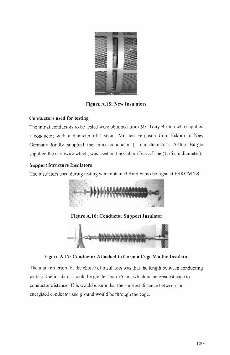
Figure A.1S: New Insulators

Conductors used for testing

The initial conductors to be tested were obtained from Mr. Tony Britten who supplied

a conductor with a diameter of 1.36cm. Mr. Ian Ferguson from Eskom in New

Germany kindly supplied the mink conductor (1 cm diameter). Arthur Burger

supplied the earthwire which, was used on the Cahora Bassa Line (1.76 cm diameter).

Support Structure Insulators

The insulators used during testing were obtained from Fabio bologna at ESKOM TSI.

Figure A.16: Conductor Support Insulator

Figure A.17: Conductor Attached to Corona Cage Via the Insulator

The main criterion for the choice of insulators was that the length between conducting

parts of the insulator should be greater than 75 cm, which is the greatest cage to

conductor distance. This would ensure that the shortest distance between the

energised conductor and ground would be through the cage.

109

Installation in the laboratory

Once the cage and support structure had been assembled in the workshop, it was dis

assembled and taken down to the HYDe laboratory where the technicians re

assembled it. Assembly and dis-assembly was made easy due to the fact that the cage

was designed and built in parts which are easily joined together. This is shown in

figure A.I8 below.

•

Figure A.IS: Laboratory Technicians attaching Cage Rings to Support Structure

Figure A.19: Completed Corona Cage in HVDC Laboratory

110

APPENDIXB

HYDC LABORATORY CONSTRUCTION

Figure B.l HVDe Laboratory Under construction

Figure B.2: Installation of the shielding mesh

111

Figure B.3: Outside view of HVDC Laboratory under Construction

Figure B.4: Outside View of Completed HVDC Laboratory

112

Figure B.5: HVDe test kit being Assembled

113

APPENDIXC

MEASUREMENT INSTRUMENTS

C.I Ammeter

The ammeter used during testing was discussed in chapter five. Below follows a detailed

diagram of the controls and jacks of this ammeter as well as a photograph of it.

CONTROLS AND JACKS

Figure C.l: Diagram of Ammeter used

1. Ohms Scale

2. DC Volts, DC Ampere Scale

3. AC Volts Scale

4. ACIDC 12 A Scale

5. dB (Decibel Scale)

6. dB Add number chart refer ACV Scale

7. Meter Zero Adjusting Screw

114

8. Range Selector Knob

9. For only DC 1000V (DC 1 kV) jack terminal plug-in connection for red test lead.

10. +ACIDC Voltages, DC Amperes and Ohms Jack Terminal, Except DC 1000V and

ACIDC 12 A measurement.

11. COM Jack Terminal, Plug-in connection for black test lead.

12. For only ACIDC 12A Jack terminal. Plug-in connection for red test lead.

13. Ohms zero adjusting knob.

14. Low AC volts Scale for AC 2.5 V range.

115

APPENDIXD

Direct Integration of Laplace's Equation: Field Between Coaxial Cylinders with

Two Dielectrics

The following is a solution for the voltage of co-axial cylinders with two dielectrics

which was modified from Ramo, Whinnery and Van Duzer [Ramo, Whinnery, Van

Duzer, 1994]

Figure D.l below is a representation of coaxial cylinders with two dielectrics.

Figure D.I: Coaxial Cylinders with Two Dielectrics

a = conductor radius

b = a + thickness of coating

c = radius of cage

8[ = permitivity of silicone

82 = permitivity of air

The inner potential at a, is Vo and the outer potential at b is 0 V.

Laplaces equation in cylindrical coordinates is as follows :

V2<D=~~(r B<D ) +_1 B2 <D + B2 <D =0 (D.l) r Br Br r2 BrjJ 2 BZ2

As stated in chapter four, due to the symmetry of the coaxial configuration the

problem reduces to a one-dimensional problem. Equation D.l therefore becomes:

~~(r B<D ) = 0 (D.2) r Br Br

Now multiplying by r on both sides and integrating we get:

116

Integrating again we have:

<Dl = Cl lnr + C2 (D.4)

This solution is valid in the first dielectric region (E l), where a < r < b. The same

equations can be used for the second dielectric region (E2)' This resultant equation is

as follows:

<D 2 = C3 lnr+ C4 (D.S)

This solution is valid region 2 where b < r < c.

Now applying the boundary conditions:

A: <DJ = Vo at r = a

B: <D 2 = 0 at r = c

These are two equations required to solve equations D.4 and D.S simultaneously.

Since we have four unknowns (Cl, ... C4) in these two equations we will need another

two equations to compliment A and B.

Continuity conditions apply at the boundary between the two dielectric media. This

says that the potential and normal component of electric flux density must be

continuous across the charge-free boundary. Therefore we have the following:

D therefore implies that GlCl = G2C2 at r = b.

Now substituting A into D.4 we get:

Vo = Cllna +C2

This implies that:

CI =VQ-C1lna (i)

Now substituting B into D.S we get:

0= C3lnr + C4

117

this implies that:

Now substituting C into DA and D.S we get:

C\lnb + C2 = C3lnb + C4

This gives us:

Substituting D into D.4 and D.S we get:

Cl = 8 2C3/ 8\ (iv)

Manipulating (iii) and equating to (iv):

C3 = (C\lnb + C2 - C4)/lnb

So:

Making C3 the subject of the fonnula:

Substituting (i) and (ii) into the above equation:

After some algebraic manipulation we get:

(*)

Once we have obtained C3 the other constants Cl, C2 and C4 are quite easy to get,

they are as follows:

118

(**)

_----,_-_v-..,-o--,-( _:~--,-J_ln_a_---;-------:- (* * *)

C2

= Vo

- (J ( J Inbx :~ -1 +lnc-lnax :~

C _ __ ----:--_---:-V__=_o _In_c ___ ---:----:-

, - In b x (:: - I J + In c - In a x ( :: J (****)

Now the initial equations can be easily solved by, substituting the known variables

into the equations for Cl, C2, C3 and C4. Then substitute these variables back into the

original equations.

Now: a = 0.88 cm, b = 0.8825 cm, c = 75 cm, 81 = 1, 82 = 2.4 and Vo = 150 kV. This

implies that Cl = -14.065, C2 = 148.202, C3 = -33.756, C4 = 145.741.

So the voltage at the surface of the coating is 149.77 kV, this means a volt drop of

0.223 kV or 230 V. So the maximum electric field gradient in the coating is 92

kV/cm.

119

APPENDIXE

Analysis of Silicone Coating for Corona Reduction

Coatings of Silicone rubber material are being evaluated to determine if their use can

reduce the problem of corona discharge. Three samples were submitted for scanning

electron microscope (SEM) analysis. They were marked as follows:

1. Mid-section small conductor (1.00 cm diameter)

2. Mid-section large conductor (1.76 cm diameter)

3. Mid-section medium sized conductor (1.36 cm diameter)

In the evaluations use is made of the material behaviour when an electron beam

accelerated to 20KV is focussed onto the sample as target. This beam is normally

under high vacuum (less than 10-4 mbar) and produces a surface charge on the sample

depending on the interaction of the beam on the sample and the capacitative and

conductive discharge mechanisms. The methods employed are not fully researched

and do not give clear quantitative data, but could help in identifying and highlighting

differences in behaviour.

EDX analysis of the samples

The samples were analysed by energy dispersive X-ray spectroscopy (EDX). The

spectra show high silicone peaks with few contaminants except aluminium (probably

from the conductor) and titanium (probably a pigment). Figure1 shows two spectra

taken on samples 1 and 2. Except for a possible small variation in titanium content,

the composition showed no significant differences in the three samples. The at the

high end of the spectrum the cut-off potential was in the range 14KV to 16KV

indicating a beam energy loss due to sample charging of about 4 to 6KV. The cut-off

potential was not clearly defined, making a comparison between the samples

subjective.

120

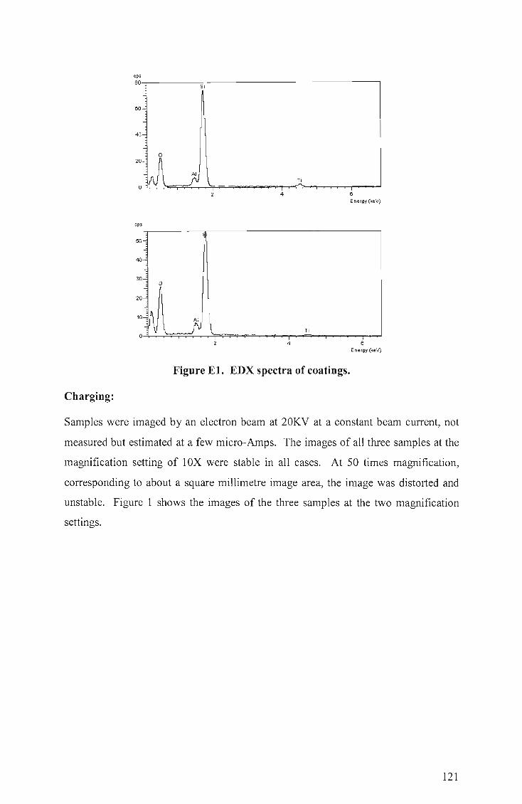
Charging:

cps

80~--------S~i -----------------------------'

60-:

cps

50-:

30..., o

20~

2 4

Ti

2 4

Figure El. EDX spectra of coatings.

e Energy (\reV)

6 Energy (\reV)

Samples were imaged by an electron beam at 20KV at a constant beam current, not

measured but estimated at a few micro-Amps. The images of all three samples at the

magnification setting of laX were stable in all cases. At 50 times magnification,

corresponding to about a square millimetre image area, the image was distorted and

unstable. Figure 1 shows the images of the three samples at the two magnification

settings.

121

Figure E2. Images at 20KV. From top to bottom samples 1 to 3. Left image at

lOx magnification, right image at 50x magnification.

Sample 2 was the least stable (most charged) image. This trend was confirmed when

the voltage was then reduced to determine the effect of the residual charge.

Sample 2 remained fully charged, deflecting the beam towards the internals of the

specimen chamber for at least 30 minutes. The deflected image was stable and

undistorted at low voltages and remained stable at voltages up to 7KV. Figures 2a to

2c show images of the secondary detector taken at l.2KV, 2KV and SKY. Figure 2d

shows an image of Sample 1 at 2KV. The latter image was highly distorted stable for

only a few minutes. The image from Sample 3 was similar. It is concluded that a

122

significant difference exists between the discharge of the three samples with Sample 2

discharging less readily than the other two.

Figure E3. Images of secondary electron detector reflected from charged

sample. Sample 2: A: 1.2KV B: 2KV C: 5KV D: Sample 1 at 2KV.

Ionic discharge

The sample chamber was filled with air at controlled pressure using the environmental

SEM facilities. This has the effect of discharging the sample due to ionic conduction

(corona discharge). The specimen charge typically dissipates as the pressure in the

partial vacuum increases beyond a particular value. These values are tabled below:

Sample number Pressure (mbar)

1 2.4

2 1.8

3 2.2

Table E.1 Pressure exerted on samples.

It can be seen that sample 2 discharged most readily in air, even though the charging

in high vacuum as determined above was more severe and more stable.

123

APPENDIXF

ELECTRIC AND MAGNETIC FIELDS

Fe! ELECTRIC FIELDS

In order to understand electric fields and field theory, it is important to understand

charge theory.

F.1.1 Electric Charge

The phenomena of two objects sticking together can be explained by the notion that

objects, when rubbed together, can gain a net electric charge. There are two types of

charge, labeled positive (+) and negative (-), with the following basic properties:

• Like charges of the same sign, repel each other.

• Unlike charges of the opposite sign, attract each other.

Detailed experiments have established the following fundamental characteristics of

electric charge:

• Charge is never created nor destroyed - it is conserved.

• Charge always comes in an integral multiple of a basic unit - it is quantized.

This basic unit of charge is conventionally denoted bye:

e = 1.602 x 10-19 Coulombs( C)

From Newton's Universal Law of Gravitation, it is known that a gravitational force

field is associated with material bodies due to their physical property, known as mass.

Newton showed that the gravitational force of attraction between two bodies of

masses, ml and m2, separated by a distance R, which is large compared to their sizes,

is equal to:

Where:

m1m2G R2

(F. 1)

ml and m2 are the masses of the objects

G is the universal gravitational constant

124

In a similar manner, a force field known as the electric field is associated with bodies

that are charged. A material body may be charged positively or negatively or may

possess no net charge at all [9] .

Alternatively, we can say that an electric charge creates an electric field in the space

surrounding it. When a second charged particle approaches the first, it reacts with it,

indirectly, through the fields created by both particles. The accepted unit of charge,

from the SI (International System), is the Coulomb (C) which, compared to the charge

of an electron (-1.60219E-19 C), is high. In fact 6.24*1018 electrons represent a

charge in one negative coulomb.

From experiments conducted by Coulomb it was shown that for two charged bodies,

which are small in size compared to their separation so that they can be considered as

point charges:

• The magnitude of the force is proportional to the square of the distance

between the charges.

• The magnitude of this force depends on the medium.

• The direction of the force is along the line joining the charges.

For free space, the constant of proportionality is 1/4 where EO is known as the / 4JZ'&o

permittivity of free space, having a value of 8.854*10-12• Now, if we consider two

point charges Q1C and Q2C separated R m in free space as shown in figure F.l, then

the forces FI and F2 experienced by Ql and Q2 respectively are given by

(F.2)

(F.3)

Where hI and i l2 are unit vectors along the line joining Ql and Q 2 as shown in the

figure below. Equations 2.2 and 2.3 represent Coulomb's law.

125

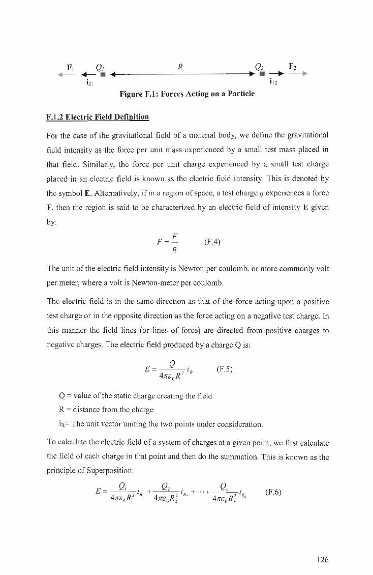
FJ QI R Q2 F2 ~ ~ . ~~~--------------------------~~ . ~ ---.

hI iJ2

Figure F.l: Forces Acting on a Particle

F.1.2 Electric Field Definition

For the case of the gravitational field of a material body, we define the gravitational

field intensity as the force per unit mass experienced by a small test mass placed in

that field. Similarly, the force per unit charge experienced by a small test charge

placed in an electric field is known as the electric field intensity. This is denoted by

the symbol E. Alternatively, if in a region of space, a test charge q experiences a force

F, then the region is said to be characterized by an electric field of intensity E given

by:

E = F (FA) q

The unit of the electric field intensity is Newton per coulomb, or more commonly volt

per meter, where a volt is Newton-meter per coulomb.

The electric field is in the same direction as that of the force acting upon a positive

test charge or in the opposite direction as the force acting on a negative test charge. In

this manner the field lines (or lines of force) are directed from positive charges to

negative charges. The electric field produced by a charge Q is:

Q = value of the static charge creating the field.

R = distance from the charge

iR= The unit vector uniting the two points under consideration.

To calculate the electric field of a system of charges at a given point, we first calculate

the field of each charge in that point and then do the summation. This is known as the

principle of Superposition:

E= Q, iR + Q2 iR + ... + Qn iRn (F.6) 4:rrcoR,2 1 4:rrc

OR; 2 4:rrcoR:

126

A way of visualizing an electric field is to spread grass seeds over a liquid, like oil,

and place two electrodes (a positive and negative) into the oil. You will see the seeds

align with the electric field.

An electric field could be defined as: "The region of space surrounding static electric

charges, which may be mapped by drawing lines of electric flux and orthogonal

equipotentiallines". These lines delineate the electric field surrounding the charges [2,

310].

F.1.3 Conductor Surface Electric Fields

The most important influencing factor in the occurrence and characteristic of corona

discharges on transmission lines conductors is the electric field distribution in the

region surrounding the conductor surfaces. In analyzing corona performance,

information, on the variation of the electric field around the conductor as well as in

the space just outside the conductor surface, is required. Electrostatic field principles

have been applied to develop accurate methods for the determination of conductor

surface electric fields of transmission lines, particularly for lines using bundled

conductors.

The corona performance of a transmission line which, is defined by effects such as,

• Corona Loss

• Radio Interference and

• Audible Noise

Depends mainly on two sets of factors:

• Line Design

• Ambient Weather Conditions

The line design factors of interest are the type and dimensions of the conductor, phase

spacing in the case of AC lines and pole spacing in the case of DC lines, and height

above ground of the conductors. The most important factor that influences the

generation of corona, however, is the electric field distribution in the vicinity of the

conductor surface.

Ambient weather conditions influence the corona performance in two ways: firstly the

temperature, pressure and relative humidity of the ambient air affect the basic

ionization processes involved in corona discharges; and secondly any precipitation

127

such as rain or snow deposited, on the conductor surface, distorts the electric field in

the vicinity.

F.1.4 The Differences between AC and DC Electric Fields

DC electric fields are different to their AC counterparts due mainly to the following

factors: DC lines generate electric fields that are constant by nature, whereas AC lines

produce electric fields, which oscillate in accordance with the frequency at which the

system operates.

AC electric fields are independent of season, climate, weather and wind, depending

only on the geometry and voltage of the conductors because they are determined only

by the charge residing on the conductors [10, 1-63]. In the case of AC lines, electric

induction effects on people and objects located near the line are produced mainly due

to capacitive coupling, and corona [5].

Due to the constant nature of the voltage on DC lines, capacitive coupling is almost

non-existent, while corona on the conductors and the resulting space charges play a

dominant role in the induction effects produced [5]. The DC electric field causes

charged particles to migrate to ground and to other objects. Voltages can therefore be

induced on insulated objects to this ionic flow [30].

DC electric fields depend in a large part on the space. The DC field though

undirectional, may slowly change as the space charge is moved by the wind. These

fields vary, greatly with weather, season and climate. The electric field at ground

potential has the polarity of the nearest conductor [10, 1-64].

The generation of air ions is peculiar to HVDC; these ions can reach concentrations

significantly above ambient values near ground, both within and outside the right of

way. This aspect of the HVDC environmental line performance is potentially the

greatest constraint on line design [10, 1-64].

Two zones surround "live" DC conductors: [12, 73]

• Ionization zone and the

• Interelectrode zone.

The ionization zone is usually 2 cm thick for pole spacings' and conductor heights of

about 15m.

128

The presence of the corona generated Space Charge phenomenon makes the electric

field and charge environment in the vicinity of DC transmission lines complex and

dynamic [6].

F.1.S Electric Fields Between Various Electrode Configurations

The formulae for calculating the electric field strength for various electrode

configurations are well known, some of them are given below.

• Parallel Plate Electrodes: If a voltage is applied between parallel plates

the electrostatic field between them will be uniform. In general the electric

field strength for this configuration is given by the following:

,r , , , v

, , , , , , , , r , r , , , , , ~~

EqUlpotentIal hnes

E=~ d

, , r , r , r , , , , ., , , , , , , , ,

... ...

Figure F.2 Parallel Plate Electrode Configuration

+ I ~~

r ,r

1,1r

-

d

Field lines

Figure F.2 above shows us the parallel plate configuration. Since the field is uniform

the electric field strength will be constant throughout the inter-electrode region. In

practical cases the field strength will be higher at the edges of the electrodes due to

the end or fringing effects.

129

• Concentric cylinders: If curved electrodes are used the electric field

strength will not be constant throughout the interelectrode region. In this

configuration the equipotential lines are much closer together near the

inner conductor than at the outer conductor. This type of electric field is

known as a non-uniform electric field.

The electric field at any point between the inner and outer electrodes is

given by the following formula:

Where a < r < b

a = inner radius

b = outer radius

~ ~ rod to plane gap ~

rod gap

• • • ~

r----...... homgap

three phase conductors

a) b)

Figure F.3: a) Field Between concentric cylinders, b) Other configurations which lead to non-uniform fields [17].

• Concentric Spheres: If a voltage V is applied between two concentric

spheres the maximum electric field strength can be found using Gauss'

Law and is as follows:

When b ~ 00, that is if the sphere is isolated then E = V , a a

130

F.2 Magnetic Fields

F.2.1 Definition of a Magnetic Field

A magnetized bar has its power concentrated at two ends, its poles; they are known as

its north (N) and south (S) poles, because if the bar is hung by its middle from a

string, its N end tends to point northwards and its S end southwards. The N end will

repel the N end of another magnet, S will repel S, but N and S attract each other,

shown in the figure below. The region where this is observed is loosely called a

magnetic field.

North attractS

repels. North

Compass needle

Figure F.4: Effect of Magnetic Poles [20].

Either pole can also attract iron objects such as pins and paper clips. That is because

under the influence of a nearby magnet, each pin or paper clip becomes itself a

temporary magnet, with its poles arranged in a way appropriate to magnetic attraction.

But this property of iron is a very special type of magnetism, almost an accident of

nature!

Out in space there is no magnetic iron, yet magnetism is widespread. For instance,

sunspots consist of glowing hot gas, yet they are all intensely magnetic. The Earth's

own magnetic powers arise deep in its interior, and temperatures there are too high for

iron magnets, which lose all their power when heated to a red glow.

F.2.2 Electromagnetism

Matter consists of electrically charged particles: each atom consists of light, negative

electrons swarming around a positive nucleus as seen in figure F.5. Objects with extra

electrons are negatively (-) charged, while those missing some electrons are positively

( +) charged.

131

Figure F.5: The atom [20].

Such charging with "static electricity" may happen (sometimes unintentionally!) when

objects are brushed with cloth or fur on a dry day. Experiments in the 1700s have

shown that (+) repels (+), (- ) repels (-), while (+) and (-) attract each other.

Close to 1800 it was found that when the ends of a chemical "battery" were connected

by a metal wire, a steady stream of electric charges flowed in that wire and heated it.

That flow became known as an electric current. In a simplified view, what happens is

that electrons hop from atom to atom in the metal [20].

In 1821 Hans Christian Oersted in Denmark found, unexpectedly, that such an electric

current caused a compass needle to move. An electric current produced a magnetic

force [20].

Andre-Marie Ampere in France soon unraveled the meaning. The fundamental nature

of magnetism was not associated with magnetic poles or iron magnets, but with

electric currents. The magnetic force was basically a force between electric currents

(figure below):

- Battery +

Pa ra 11 e 1 cur re nts att ract eac h ot he r

Battery +

'---------'

Figure F.6: Force Between Two Electric Currents [20].

Two parallel currents in the same direction attract each other

132

Two parallel currents in opposite directions repel each other.

Here is how this can lead to the notion of magnetic poles. Bend the wires into circles

with constant separation:

PElrElll e 1 currents in two lOORS Ell so ElttrElct

Figure F.7: Two Magnetic Loops [20].

• Two circular currents in the same direction attract each other.

• Two circular currents in opposite directions repel each other.

Replace each circle with a coil of 10, 100 or more turns, carrying the same current

(figure below): the attraction or repulsion increases by an appropriate factor.

s N s N Two coils of many parallel loops, with currents in the same di rect i on, attract each other and act like magnets

Figure F.8: Magnetic Coils [20].

In fact, each coil acts very much like a magnet with magnetic poles at each end (an

"electromagnet"). Ampere guessed that each atom of iron contained a circulating

current, turning it into a small magnet, and that in an iron magnet all these atomic

magnets were lined up in the same direction, allowing their magnetic forces to add up.

The magnetic property becomes even stronger if a core of iron is placed inside the

coils, creating an "electromagnet"; that requires enlisting the help of iron, but is not

essential. In fact, some of the world's strongest magnets contain no iron, because the

added benefit of iron inside an electromagnet has a definite limit, whereas the strength

133

of the magnetic force produced directly by an electric current is only limited by

engineering considerations.

In space, on the Sun and in the Earth's core, electric currents are the only source of

magnetism. We loosely refer to the region of their influence as their magnetic field.

Figure F.9: The Earth's Rotation Inducing a Magnetic Field [20].

F.2.3 Differences between AC and DC magnetic fields

AC magnetic fields are alternating in nature and capable of inducing currents in

circuits and conductive bodies. The magnetic field of DC lines is similar to the earth's

magnetic field. These magnetic field values generally, do not exceed the value of the

earth's field and have not been associated with any biological or health effects for

people [10, 1-64].

The earth's natural magnetic field, ranges from 30 to 70 ).lTeslas(T) depending on the

location of the measurement. Magnetic fields under HVDC transmission lines, which

are static in nature, are typically of the order of20).lT [13, 3].

F.3 SUMMARY

Electric charge is never created or destroyed, electric charge always comes in an

integral multiple of a basic unit. Like charges repel each other and unlike charges

attract each other. The basic unit of charge is the Coulomb (C).

Electric field intensity is measured in Newtons per Coulomb or more commonly in

Volts per Meter. The electric field is in the same direction as that of the force acting

upon a positive test charge or in the opposite direction of the force acting upon a

134

negative test charge. This means that field lines are directed from the positive charge

to the negative charge.

Electric field distribution III the regIOn surrounding the conductor is the most

important factor, influencing the occurrence and characteristics of corona discharges

on transmission lines.

DC electric fields differ from AC electric fields in that DC transmission lines generate

electric fields which are static in nature whereas AC transmission lines generate

electric fields which oscillate in accordance with the frequency at which the system in

question operates.

Electric fields can be broken up into two sets, these are:

• Uniform fields and

• Non-uniform fields

Electric currents can cause magnetic fields to occur. Two parallel currents in the same

direction attract each other and two parallel currents in the opposite direction repel

each other.

AC magnetic fields are alternating in nature and capable of inducing currents in

circuits and conductive bodies. DC magnetic fields are similar to the earth's magnetic

field. The DC field magnitude generally does not exceed the earth's magnetic field

values.

135

a study of high voltage direct current conductor corona …

Documents