a study of combining technique of single-dish and ...lib_pub/html/report/data/tno73.pdf ·...

PASJ: Publ. Astron. Soc. Japan , 1–??,c© 2009. Astronomical Society of Japan.

A Study of Combining Technique ofSingle-Dish and Interferometer Data:

Imaging Simulations and Analysis

Yasutaka Kurono∗,1,2 Koh-Ichiro Morita,2,3 and Takeshi Kamazaki31Department of Astronomy, Graduate School of Science, The University of Tokyo, 7-3-1 Hongo, Bunkyo, Tokyo 113-0033

[email protected] Radio Observatory, National Astronomical Observatory, 462-2 Nobeyama, Minamimaki, Minamisaku, Nagano

384-13053ALMA-J Project Office, National Astronomical Observatory, 2-21-1 Osawa, Mitaka, Tokyo 181-8588

(Received 2008 October 26; accepted 2009 May 17)

Abstract

We have investigated the technique of combining single-dish data and interferometer data in the spatialfrequency domain, using imaging simulations and analytical considerations. Our study shows that there isan optimum of relative weights between the visibility data of single-dish and interferometer. The qualityof the reconstructed combined image achieves the highest at the relative weights where the mean of thedifference between the synthesized beam and the CLEAN beam is close to zero. We also examined the(u,v)-range that can be effectively used for the data combining by considering the blurring effect due topointing error. The error in single-dish deconvolution caused by the beam approximation is small witha large diameter of the single-dish aperture. The diameter should be at least 1.7 times larger than theminimum baseline of the interferometer for the amplitude accuracy better than 10%. Furthermore, wederived an estimate of the noise variance in the combined image, which agrees with our simulation results.The noise-added simulations demonstrate that there is a threshold of the noise level of the single-dishimage, beyond which a large-scale error is emphasized in the combined image. We should take observationtimes to make at least same noise level at the border of spatial frequency between the single-dish andinterferometer. Although our examinations were assumed to use 45m Telescope and NMA, our results ofthe required conditions for observations and data processes can be used in a general case of heterogeneousarray imaging.

Key words: methods: data analysis — techniques: image processing

1. Introduction

In radio astronomical observations, single-dish telescopes or interferometers are used according to the spatial scaleof target sources and scientific purposes. Single-dish observations are often used in mapping of a wide region on thesky, while interferometer observations can achieve a higher spatial resolution compared to single-dish observations.

In interferometric observations, visibilities are measured on the spatial frequency plane ((u,v)-plane), at points alongthe projected baselines of antenna spacings in the range from the minimum baseline Bmin to the maximum baselineBmax. The distribution of visibilities is usually referred as “(u,v)-coverage” (see Thompson et al. 2001). In general,the lowest spatial frequency sampled with an interferometer is constrained by the physical limitations in placing twoantennas together and shadowing effects of one dish by another. For example, the Nobeyama Millimeter Array (NMA)at the Nobeyama Radio Observatory (NRO)1, whose primary antennas have a diameter of Dint = 10m, can measurespatial frequencies down to a spacing of Bmin = 10m.

This incompleteness of (u,v)-coverage results in a degradation of the synthesized images, causing structures suchas negative bowls around emission components, and sidelobes (Cornwell et al. 1999). Image affected by these can bepartly restored by image reconstruction techniques such as CLEAN (Hogbom 1974), or Maximum Entropy Method(MEM) (e.g., Narayan & Nityananda 1986), that interpolate or extrapolate missing information in the (u,v)-plane.Nevertheless, it is difficult to reconstruct synthesized images with emission components of size larger than ∼ λ/Bmin,where λ is the observation wavelength. The lack of information in the center of the (u,v)-coverage is often referred toas the “short spacing problem”. This short spacing problem makes extrapolating the zero baseline difficult, and results

∗ Present address: ALMA-J Project Office, National Astronomical Observatory, 2-21-1 Osawa, Mitaka, Tokyo 181-85881 Nobeyama Radio Observatory is a branch of the National Astronomical Observatory, National Institutes of Natural Sciences, Japan.

2 Kurono et al. [Vol. ,

in “missing large-scale flux”. In many cases of scientific purposes, it is essential to obtain higher spatial resolutionobservations of larger objects, and to accurately depict the structures over a wide range of spatial scales.

On the other hand, scanning a single-dish telescope across a celestial object samples spatial frequencies over therange from zero spacing to the maximum baseline corresponding to the antenna diameter Dsd. Thus, if the antennadiameter of the single-dish telescope is larger than the interferometer’s minimum baseline, one can make an imageof a target source using spatial information over the range of 0−Bmax by combining single-dish and interferometerdata. Combining methods are currently widely used and can be roughly classified into two kinds, data combining inthe image domain (Schwarz & Wakker 1991; Stewart et al. 1993; Holdaway 1999; Stanimirovic et al. 1999) and in thespatial frequency domain (Bajaja & van Albada 1979; Vogel et al. 1984; Wilner & Welch 1994; Zhou et al. 1996).

At NRO, data combining of the 45m Telescope and NMA in the (u,v)-domain has been popular to obtain radioimages of spatially high-dynamic range (Takahashi et al. 2006; Takakuwa et al. 2003), since the study by Takakuwa(2003) was published. This technique has the advantage of being conceptually easy, but requires determining severalempirical parameters for observations or data processes. (e.g., weight ratio between single-dish and interferometerdata). Moreover, combined result includes observational errors which have different properties between single-dishand interferometer observations. Although an experimental analysis for these issues has been partially done (Saito2007), more detailed and scientific investigations using analytical and simulation approaches are needed to improvethe qualities of the results. The purpose of this study is to examine these parameters, using imaging simulations andanalytical considerations. We expect that some important suggestion can be made not only for the NRO case but alsogeneral cases of heterogeneous array imaging.

In this paper, we present an analysis of imaging with combining single-dish and interferometer data in spatialfrequency domain, and step-by-step data processing following this principle (§2). Among the issues that should beclarified for this technique, we concentrated in the study of the optimization of relative weights of single-dish andinterferometer data (§4), the influence of error included in single-dish data (§5), and the problem of sensitivity in thecombining process and results, including the relation to the quality of the combined images (§6).

2. Combining Single-Dish and Interferometer Data

In this section, we describe a theoretical expression of the handling of a single-dish image required to implementthe data combining in the (u,v)-domain, and show the actual data processing.

The weighted visibility function sampled by interferometer observations is written as

VI(u,v) = [V (u,v) ∗ ∗pI,pr(u′,v′)] ·wI(u,v), (1)

where ∗∗ denotes two dimensional convolution, pI,pr is the Fourier transform of the response pattern of the interferom-eter primary antenna PI,pr, wI is the weighted sampling function (Briggs et al. 1999), and V is the Fourier transformof the true brightness distribution I(l,m).

On the other hand, the observed brightness distribution of single-dish observations can be written as

IS(l,m) = [I(l,m) ∗ ∗PS(l′,m′)] ·SS(l,m), (2)

where PS is the beam pattern and SS is the spatial sampling function on the sky. The Fourier transform of Equation(2) results in

VS(u,v) = FIS(l,m)= [V (u,v) · pS(u,v)] ∗ ∗sS(u′,v′), (3)

where pS and sS are the Fourier transforms of PS and SS, respectively. Although the spatial sampling SS is in principlearbitrary, we assume a series of delta functions (Bracewell & Roberts 1954, the Shah function) with intervals of ∆land ∆m for simplicity:

SS(l,m) = III(l/∆l,m/∆m)

=∞∑

j=−∞

∞∑k=−∞

δ(j − l/∆l,k−m/∆m), (4)

and its Fourier transform sS is also a Shah function,

sS(u,v) = III(u∆l,v∆m)

=∞∑

j=−∞

∞∑k=−∞

δ(j −u∆l,k− v∆m). (5)

It is necessary to estimate the true visibility from Equation (3) to be combined with the interferometer data.When the sampling interval of the single-dish image is less than λ/2Dsd, the Nyquist spacing, aliasing caused by the

No. ] A Study of Combining Technique 3

convolution in Equation (3) will not distort the true visibility (e.g., Vogel et al. 1984). Hence, the true visibility canbe obtained by

V (u,v) =VS

pS(u,v). (6)

Next, we can obtain the spatial frequency data by convolving the visibilities in Equation (6) by the primary beam ofthe interferometer and re-sampling,

V ′S(u,v) = [V (u,v) ∗ ∗pI,pr(u′,v′)] ·wS(u,v), (7)

where wS(u,v) is the weighted sampling function uniformly distributed for the single-dish data. Finally, from Equation(1) and (7) the combined visibility data set can be written as

VI(u,v)+ V ′S(u,v)

= [V (u,v) ∗ ∗pI,pr(u′,v′)] · [wI(u,v)+ wS(u,v)]= [V (u,v) ∗ ∗pI,pr(u′,v′)] ·wI+S(u,v). (8)

The function wI+S(u,v) is the weighted (u,v)-sampling function for combining the single-dish and interferometer data.The combined image can then be obtained by routine imaging procedures (Briggs et al. 1999). The synthesized beamis represented as the point source response, and should be given by FwI+S. The weights applied to the (u,v)-samplingpoints of the single-dish and interferometer data, wI and wS play a crucial role on the combined image to be obtained,and image reconstruction later.

Figure 1 shows the data processing flow used in this report. Data processing was done using the MIRIAD package(Sault et al. 1995). First, to estimate the true brightness distribution of the source, we deconvolved2 the single-dishdata by filtering the VS in Equation (6) through the reciprocal of transfer characteristics of the single-dish observations.We used a Gaussian pattern with the same full width at half maximum (FWHM) of the observing beam. Next, weexecute Equation (7); the deconvolved image as a result of Equation (6) is multiplied by the primary beam pattern ofthe interferometer observation, and we obtain the visibility data by applying an uniformly distributed (u,v)-samplingpoints to the Fourier transform of the single-dish image passed through such processes. Since the shortest spatialfrequency the NMA can measure is 10m, we generated the visibility data uniformly from the single-dish image in thespatial frequency range of 0−10m, in which wS is distributed. In this paper, we refer to this area in the (u,v)-domainas “complement region”.

In addition, it is necessary to confirm that the intensity scales of both data of the interferometer and single-dish inthe (u,v)-domain are consistent with each other before the data combining. Actual observed data do not often agreemainly due to different quality of data or/and accuracy of calibrations. This results in a discrepancy in the measuredflux densities. If the diameter of the single-dish telescope is larger than the minimum baseline of the interferometer,there is a common (u,v)-area in which both of the instruments measure the visibilities. In principle, the consistencybetween two data sets can be checked in this region. We define the “overlap region” as the (u,v)-area where the single-dish and interferometer data can be compared. If needed, either of the data should be adjusted to the amplitude ofthe other (relative flux calibration or cross-calibration). For the combination of the 45m Telescope and the NMA, theoverlap region is 10− 35m. The reason not to use up to 45m is as follows. The support for the visibilities VS(u,v)in Equation (6) is 0− 45m and so is that of for V (u,v) in Equation (7). Nevertheless, the support for the Fouriertransform of the interferometer primary beam, pI,pr, in the (u,v)-domain is ±10m. Thus, after the convolution inEquation (7), at the (u,v)-distance of 35− 45m the visibilities estimated from the 45m Telescope data do not includethe information of 45−55m. Thus, we cannot compare the NMA and 45m visibilities at the (u,v)-distance of 35−45m.The left panel of figure 2 shows the (u,v)-coverage after the combining process, in which green and blue show the(u, v)-coverage of NMA and that in the overlap region, respectively, and red shows the visibilities generated fromthe 45m Telescope data in the complement region. The right panel of figure 2 shows an example of the visibilityamplitude obtained with NMA and generated from 45m Telescope data, for the case of no observational error andnoise-free (§4.2).

Note that there are several issues in the data combining method. There are parameters which would give importantinfluence to resultant image but those effects have not been studied in detail. First, we discuss the issue of therelative weights between the interferometer and single-dish data, wI and wS. The weights applied to the visibilitydata are reflected in the resulting images directly, and it is important to examine their influence on a nonlinear imagereconstruction process. Secondly, considering that the single-dish data undergoes various data processings, we should2 The “deconvolution” process on MIRIAD (task “convol” with “options=divide”) uses Wiener filtering with a transfer function:

TWF(u,v) =H∗(u,v)

|H(u,v)|2 + sigma2,

where H is the transfer characteristic of the observation, that is, the Fourier transform of the observing beam. The parameter “sigma”is to control a contribution of added noise to the restored signal.


investigate how the error of response in single-dish observations, for example, pointing error and uncertainty of thebeam shape, influence the data combining. Thirdly, we examine the required sensitivity for both data sets to obtaingood results. This is important for the planning of observations with the combining method. In addition, it is necessaryto consider the influence of the noise or observational error on the cross-calibration in the actual data processing.

3. Imaging Simulations

The purpose of this paper is to examine the practical issues mentioned in the previous section. In this section, wesummarize the methods and parameters for the imaging simulations used in this study.

All simulations were assumed to use the NRO 45m Telescope and the NMA. Detailed parameters of these simulationsare listed in table 1. At the frequency adopted in this study, 86.75433GHz, the typical beam sizes of the 45m Telescopeand the NMA primary antenna are, respectively, 18′′.5 and 79′′, and the 45m and 10m antenna diameters correspondto spatial frequencies of 13.0kλ and 2.89kλ, respectively. Thus, the (u, v)-ranges of the “complement region” and“overlap region” are 0−2.89kλ and 2.89−10.1kλ, respectively. In this simulation study the two model sources shownin figure 3 were used. These sources are placed at the center of the single-dish observing region and the field of view ofthe interferometer (i.e., the phase reference center). For the simulations of single-dish observations, we used either acircular Gaussian antenna beam with FWHM of 18′′.5, or by Fourier transforms of antenna illumination distributions(§5.2). The size of the image acquired was four times as large as the primary beam width of the NMA, ∼ 320′′×320′′,to reduce the intensities to zero at the edges of image by the primary beam in the data combining process, whichis necessary to avoid edge-effect when Fourier transforming. When using the 18′′.5-beam, the grid spacing of 7′′.75can be regarded to satisfy the Nyquist sampling criterion (§2). In the simulations of interferometer observations themodel source was multiplied by the primary beam, and visibilities were sampling out of the Fourier transform of theresult. We did not include periodic interruptions for the observations of a reference calibrator, so that the simulationsrepresent an ideal case.

When including thermal noise (§6), for the simulations of single-dish observations, we added a noise componentwhose rms level ∆T sd is given by

∆T sd =T sd

sys

ηsw

√tsd∆ν

(9)

in each pointing, where Tsys, ηsw, tsd, and ∆ν are a system temperature, a switching efficiency, an integration timeper pointing, and a frequency width, respectively. For the simulations of interferometer observations, rms noise levelat each measured point in the (u,v)-domain is determined by

∆Sintvis =

√2kBT int

sys

ηinta ηcAint

√tintvis∆ν

, (10)

where kB, ηa, ηc, A, and tintvis are, respectively, a Boltzmann constant, an aperture efficiency, a correlator efficiency, a

physical collecting area of aperture, and an integration time per visibility. The values we adopted are summarized intable 1. The achieved noise level of the interferometer observations is ∆Sint

vis = 25.5Jy, and the rms noise level of thesynthesized image is ∆Sint

im = 0.11Jybeam−1 (SNRint ∼ 34) that is given by

∆Sintim = ∆Sint

visNintvis

−1/2, (11)

where N intvis is a total number of the interferometer visibility samples, which are common in this study as the integration

time at each (u,v) measured point and the source tracking time are fixed.We always applied the natural density weight in imaging process to maximize the imaging sensitivity. We did not

apply other weighting, for instance, weighting by estimated noise-variance or tapering, to the visibility data. Theweighting function in the (u,v)-plain just corresponded to the number density distribution of visibility points. Thusthe visibility density distribution in the (u,v)-plane directly controls the synthesized beam, and greatly influences theresulting synthesized image. We used the SDI CLEAN (Steer et al. 1984) algorithm for the reconstruction of thesynthesized images, because normal CLEAN is often unstable for extended sources (Schwarz 1984). The thresholds tostop the iterative image reconstructions were set to 1% of peak flux density of the dirty image in the noise-free cases(§4, 5), and rms noise level in the noise-added cases (§6).

We applied fidelity as an indicator to assess the quality of the result of data combining. This metric was introducedfor the wide field imaging study of ALMA (Pety et al. 2001). The image and (u,v)-fidelities are calculated at eachpixel on the image and each spatial frequencies following definition:

Fidelity(i, j) =abs(Model(i, j))

abs(Model(i, j)−Combined(i, j))(12)


For the fidelity to represent the mean quality of a result, extremely high fidelity points are excluded as described inPety et al. (2001). We use the median fidelities at the intensity cutoff of 1% of the peak intensity for the noise-freesimulations (§4) and of 3% for the noise-added simulations (§6).

4. Relative Weight of the Single-Dish Data

4.1. The Combined Synthesized Beam

First, we present the effects of the weighting applied to the single-dish visibility at the “complement region” on thecharacteristics of the combined synthesized beam.

As a parameter to indicate the weight ratio of single-dish data to interferometer data, we use the density ratioβ = dsd/dint, where dsd (kλ−2) is the number density of visibility samples generated from the single-dish image, anddint is average number density of interferometer visibility samples,

dint =N int

vis

π(b2max − b2

min)(13)

where bmax = Bmax/λ and bmin = Bmin/λ. In our simulation study, the total number of interferometer visibility datawas fixed and the number density was almost constant, dint ∼ 7.6kλ−2. We varied the density of single-dish visibilitydsd from zero (imaging with the interferometer visibility only) to 300 kλ−2 (β ∼ 40) (thus, the “total weight” ofcombined visibility data set increases with β). Figure 4 show the variation of synthesized beam obtained by combiningdata for different β. It is found that nearby sidelobe levels and wing levels of the main lobe of the synthesized beamrise gradually when adding the single-dish visibility. Figure 5-(a) shows the size variation of the combined synthesizedbeam (estimated by fitting a two-dimensional Gaussian function, that is the CLEAN beam) as a function of β. Thebeam size is increasing with the weight of the single-dish visibilities. Both major and minor axes have the same rateof growth, so that the beam shape is not deformed. Moreover, the rate of increase of the beam size does not dependstrongly on the source declination. Figure 5-(b) shows the mean of the residuals for subtracting the CLEAN beamfrom the combined synthesized beam as a function of β. The mean value of the residual shows that adding the shortspacings lifts the whole of the beam up in the positive direction.

All the behavior of the combined beam variation can be understood by considering the linear combination of thesynthesized beams corresponding to the weight distribution in the (u, v)-domain of the interferometer and single-dish data. In this case, the beam shape determined only by the weight distribution of the single-dish visibilities is theFourier transform of a circular uniform distribution with the spatial frequency radius of Bmin. Thus, the beam shape isrepresented as 2J1(x)/x, where J1 is the 1st-order Bessel function of the first kind, x=π(2Bmin/λ)r, and r =

√l2 +m2.

This beam has a FWHM of ∼ 0.7λ/Bmin ∼ 50′′ and positive level at r ≤ 43′′. Because the interferometer beam is liftedby this 50′′-beam, it is evident that the mean of residual should increase to the positive direction. Additionally, thesize of synthesized beam grows because by lifting the interferometer beam by the 50′′-beam; the size of the half-powerof the combined beam corresponds to the size at lower level of synthesized beam only of the interferometer. If thesingle-dish data is extremely weighted, the contribution of the 50′′-beam will reach the half-power, and the size of thecombined beam will be decided by the 50′′-beam. However, such a situation that the weight of the single-dish data isenlarged too much will not happen.

4.2. Effect of Relative Weight on Imaging

We examined the quality of reconstructed images in the case noise-free simulations. The parameters used for thesimulations are as described in §3. We used the Gaussian 18′′.5-beam for the single-dish observations. In this case,there is no error concerning the beam efficiencies in the single-dish observations, so that the visibility of the modelsource is reproduced completely without relative flux calibration. The final combined image depends on the relativeweight setting of single-dish data.

Figure 6 shows examples of combined dirty images, reconstructed images, and difference images from model image(multiplied by the primary beam and convolved with the CLEAN beam), for different weightings of the single-dishdata β = 1/2, 5, and 20. Because the natural density weight is applied, as β is increased the large-scale structure isemphasized in the dirty images. It is found that the large-scale structure in the images is not reproduced enough atβ = 1/2, but can be recovered at β = 5, 20. However, a systematic error with structure appears in the case of β = 20,which is similar to the synthesized beam pattern. This false structure is considered to be caused by the interaction ofthe source structure with the synthesized beam.

Figure 7-(a) shows the median image fidelity with cutoff level of 1% as a function of β. Similar plots of (u,v)-fidelitiesfor the complement region (≤ 2.89kλ) and outer region (> 2.89kλ) are shown in figure 7-(b) and -(c), respectively.As a result of investigation of the fidelity for four different source declinations (left panels of figure 7) and sourcemodels (right panels of figure 7), it is clear that the quality of combined image reaches a peak at β ∼ 3− 8 in allcases. Especially, the (u,v)-fidelity of the complement region has a strong peak within this range of β. Although the


(u,v)-fidelity of the outer region does not have such a strong peak, it has a similar behavior. Figure 7-(d) show thefraction of total flux recovered. The plots show that correct total fluxes are recovered early in the range of β ∼ 4− 8.Total flux is underestimated when the weight of the single-dish data is smaller, and overestimated when it is larger.Figure 7-(d) right panel shows that the behavior of the total flux does not depend on the source size nor shape. Hence,the slight difference of the total flux behavior shown in the left panel of figure 7-(d) is solely due to the difference ofthe source declination. It is suggested that optimum β changes depending on the source declination, in other words,the shape of synthesized beam.

The fidelities of the two (u,v) ranges show that an optimization of the relative weight is important not only foraccurate recovery of a large-scale structure but also for small-scales. Taking into account the described behavior ofthe fidelity and the fraction of total flux recovered, we find that the quality of the reconstructed image combinedwith the weight setting of around β = 5 is the best. By comparing figure 7 with figure 5-(b), it can be seen that thefidelity medians are maximized when the mean of the difference between the synthesized beam and the CLEAN beamis almost zero. Moreover, the weight ratios β at which the fraction of total flux recovered equals to unity in figure7-(d) are well correlated with the zero-crossing β in figure 5-(b) for each source declination. This suggests that it isessential to use a combined beam that has no bias for positive or negative in the difference between the synthesizedbeam and the CLEAN beam. Therefore, one should apply weights at which the average of the difference between thesynthesized beam and the CLEAN beam is zero when combining the data of single-dishes and interferometers. Finally,we wish to note that we obtained similar results when using the MEM algorithm for the image reconstruction.

5. Effect of Single-Dish Response Accuracy

In this section we address the repercussions of observational, non-thermal errors included in the single-dish data.We discuss the influence of pointing errors in observations and difference between the Gaussian beam and the actualbeam shape when the single-dish image is deconvolved on the data combining.

5.1. Effect of Pointing Errors in Single-Dish Observation

Pointing errors in single-dish observations is usually caused by the wind or sunshine (daytime observations) andleads to an error in the observed maps. It is important to examine how this error affects the data combining. Wesimulated single-dish observations without thermal noise, including random pointing errors of 3′′, 6′′, and 9′′ rms withGaussian distributions, which are respectively 16%, 32%, and 49% of FWHM of the single-dish beam. The single-dishimages toward the spherical model of a single map and average of 10 maps, are shown in left panels of figure 8. To seethe influence of the pointing errors, we examined the error in visibilities and dirty images without cross-calibration orimage reconstruction.

The right panels in figure 8 show the difference images between the combined images obtained by using the averagedsingle-dish images with and without pointing error. There is a tendency to underestimate the emission strength inthe central part, and to overestimate in the outside. This means that the combined image is blurred and a large-scaleerror is produced. Nevertheless, the error fraction in the image is not large (figure 9). A random pointing error of 9′′rms is too large in a realistic situation, but even so, the error that is caused in the image is 2% rms or less and in theestimate of total flux is about 7%.

Figure 10 shows examples of the distribution of the visibility amplitude obtained through the combining process.In the complement region, the source flux tends to be underestimated and scattered faintly as the pointing accuracyworsens. On the other hand, a large error appears at higher spatial frequencies in the overlap region, and this tendencybecomes significant with the larger pointing error. Since a single-dish image is practically obtained by averaging twoor more maps, the extreme scattering at the high spatial frequencies due to the contingency of pointing error can besuppressed to some degree by averaging, as seen in middle panels of figure 10. However, the amplitude of single-dishdata tends to be underestimated up to the spatial frequency of ∼ 6kλ where the suppression of the error works well.

The observed behaviour in the (u,v)-domain are explained as follows. As seen in figure 8, small scale structures arecaused by the pointing error in the single-dish maps. It is supposed that the pointing error works to convert a fractionof large-scale flux into small-scale flux. As an effect on the visibilities at higher spatial frequencies the structure ofthe small scale can be expected basically as random just like noise. We should note that these components becomea significant error because of the amplification by deconvolution, as shown in figure 10. Besides, at lower spatialfrequencies, because flux is removed, the derived visibility function is underestimated and is narrower than truefunction; thus works to blur the image. If the pointing error is normally distributed with the variance of σ2

pe, the

effective beam size in the single-dish observation grows into√

θ2S +8ln2σ2

pe, where θS is beam size of the single-dish observation. This data is deconvolved with a Gaussian beam whose response function in the (u, v)-domain isexp(−π2θ2

Sb2/4 ln2), so that deconvolved data is underestimated by a factor of exp(−2π2σ2peb

2). This distribution isshown as dotted lines in bottom panels in figure 10, and simulated results follow closely these lines up to ∼ 3−6kλ. Ifmore maps are averaged, the scattering at the high spatial frequencies will be suppressed and the amplitude ratio will


follow this line toward higher spatial frequencies that is independent of the source structure or antenna diameter ofthe single-dish telescope. If the error that originates in this blurring effect can be allowed to εpe,blur, the pointing errorand the (u,v)-distance which can be effectively used have the relation of σpebeff ≤

√− ln(1− εpe,blur)/(2π2). When

εpe,blur = 10%, we obtain σpebeff . 7.3× 10−2. In the case of the combination of 45m Telescope and NMA, in order toguarantee the accuracy of the complement region, the pointing error should be better than 5′′.2 rms.

To summarize, out analysis suggests that the error in the combined images caused by single-dish pointing erroris not large in the case of combining NRO 45m data with NMA data. However, the effective (u, v)-range for thecross-calibration is limited due to the small scale errors caused by the pointing error. This effect is mitigated byaveraging several single-dish maps.

5.2. Using Non-Gaussian Beams for Single-Dish Observation

We usually use a Gaussian beam pattern to deconvolve the single-dish image although the beam shape in single-dishobservations is generally not an ideal Gaussian; the main reason for this is that it is not realistic to measure theaccurate beam pattern for each observation. The difference between the single-dish beam and Gaussian pattern in the(u,v)-domain causes an error in the combined image.

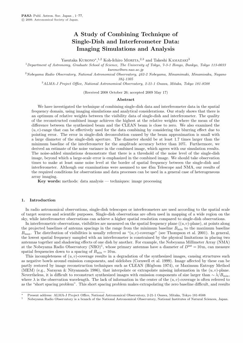
We created a couple of models of the electric field distribution of a single-dish telescope and simulated the beamsby Fourier transform of them (figure 11). We included blocking patterns by the sub-reflector and stay of two kinds,the “quadripod support” and the “tripod support”. The grading function of the illumination pattern is g(%) =K + [1− (2λ%/Dsd)2]p (Christiansen & Hogbom 1985), and we adopted K = 0.03 and p = 1 which give a beam sizesimilar to that of 45m Telescope. The parameters of the beams are summarized in table 2.

Figure 12 shows the comparison of the transfer functions, which are the response patterns in the (u,v)-domain or theautocorrelations of the illumination distribution of the aperture, of the model beams and Gaussian patterns that havethe same FWHMs as the model beams. For both stay types, the model beams can be approximated by a Gaussianpattern in the (u,v)-range of ≤ 8kλ. However, there is a conspicuous difference at higher spatial frequencies. Thus,as in §5.1, the difference of the actual observing beam from an ideal Gaussian is not a crucial problem in making thesingle-dish visibility in the complement region; however, there is a strong possibility that a remarkable error is includedin the overlap region. To investigate this, we actually simulated the single-dish images by using these model beams,and when combining with the interferometer data, the single-dish image was deconvolved with a Gaussian pattern ofthe same FWHM. The error in the resultant image is extremely small, ∼ 0.3% in peak flux density and ∼ 1% in totalflux.

In this simulation, a maximum (u,v)-distance of ∼ 8kλ can be used if relative flux error better than 10% is permittedin the cross-calibration, which corresponds to ∼ 60% of the antenna diameter of 45m Telescope. This suggests that adiameter of single-dish aperture at least larger than 1.7Bmin is required for data combining with 10% deconvolutionerror caused by the uncertainty of beam shape.

6. Thermal Noise in Combined Imaging

In this section, we discuss the quality of the combining results including thermal noise. Because the single-dish datais deconvolved and multiplied by the primary beam of the interferometer in the data combining process, it is necessaryto consider these influence. First, we will address analytically the contribution of the thermal noise in the single-dishdata to the combining process, and derive the expression of the noise variance in the combined image. For the firstpart of the analysis (§6.1), we adopt an approach using the statistical Rayleigh distribution, which is comprehensibleand is easier to derive the noise propagation. For the latter part of the analysis (§6.2), the direct pixel-based analysisis used and is the simplest way to examine the point source sensitivity. The validity of the analytical formulae willthen be confirmed by comparing with simulations including thermal noise. Finally, the quality of the combined imageafter a nonlinear image reconstruction process will be discussed from the viewpoint of the sensitivity balance in the(u,v)-domain.

6.1. Contribution of Single-Dish Noise

As shown in §2, the process of estimation of the single-dish visibilities, from IS to V ′S, is not a simple case of

Fourier transform. We examined the noise distribution of the Fourier transform of the single-dish image and that aftercombining process which includes deconvolution with the single-dish beam and multiplication by the primary beamof the interferometer. Figure 13 shows the distribution of the single-dish noise amplitude in the (u,v)-domain, forthe original data (black dots) and after deconvolved and multiplied by the primary beam (red and blue dots). Notethe independency of the visibility data in this figure. Although the visibilities represented by black and blue pointsare data on the grid points, those represented by red points are on arbitrary sampling points made by interpolationfrom the data on surrounding grid points. Therefore, the red visibilities are not independent each other, and moredetailed explanation is shown in §6.2. As can be seen in the figure, the noise appears to decrease (wrt the originalnoise amplitude) in the complement region (red) and increase significantly at high spatial frequencies (blue). The peak


of amplitude distribution which is ∼ 1Jy in the original data falls to ∼ 0.2Jy in the visibility data to be combined.Deconvolution is done by dividing by the Gaussian pattern on the (u,v)-plane so that spatial components at higherfrequencies are more amplified. However, the average amplification factor by this is only ∼ 1.13 in the complementregion of the low frequencies. On the other hand, multiplying an image by the primary beam is convolution inthe (u, v)-plane, which is data averaging over the area of the primary beam. Consequently, the noise level in thecomplement region lowers more than that of the original data.

We treat now analytically the behavior of single-dish noise. The notations in the analysis through this §6.1 andnext §6.2 are summarized in table 3 and table 4. For a noise εsd in a single-dish image and using Parseval’s Theorem,the complex noise εsd in the visibility data Fourier transformed from the single-dish image is

N∑n=1

∣∣εsdn ∣∣2 =1N

N∑m=1

∣∣∣εsdm

∣∣∣2 , (14)

We assume a square single-dish image with a size L2 and Nyquist grid intervals λ/2Dsd, thus the number of datapoints in the grid is N = L2/(λ/2Dsd)2. The noise variance of the single-dish image is ∆Ssd

pix2 (Jypixel−1), so that

the left-hand side of Equation (14) is interpreted as N∆Ssdpix

2.Assuming the noise in the single-dish observations is a Gaussian distributed white noise, we expect that the proba-

bility distribution of the amplitude∣∣∣εsd

∣∣∣ will be a Rayleigh distribution,

f(∣∣∣εsd

∣∣∣)=

∣∣∣εsd∣∣∣

σsd2 exp

−∣∣∣εsd

∣∣∣22σsd

2

. (15)

Given N independent and identically distributed Rayleigh random variables, the maximum likelihood estimate σsd =〈Re[εsd]2〉 = 〈Im[εsd]2〉 is

σsd =

√ 12N

N∑m=1

∣∣∣εsdm

∣∣∣2. (16)

Thus the right-hand side of Equation (14) can be rewritten as

1N

N∑m=1

∣∣∣εsdm

∣∣∣2 = 2σsd2. (17)

Therefore, we obtain the following relation between single-dish noise variance in the image and that in the spatialfrequency domain,

σsd2≈ N

2∆Ssd

pix

2. (18)

To deconvolve with the single-dish beam, the visibilities have to be divided by the Fourier transform of the single-dish beam (§2). Using a Gaussian pattern as the deconvolving beam, the noise in the deconvolved data εsd

′has a

standard deviation as a function of (u,v)-distance b of:

σsd′(b) = σsd exp

(π2θ2

Sb2

4ln2

), (19)

where θS is FWHM of the single-dish beam.In the next in the process, we convolve the single-dish data with the Fourier transform of the primary beam of the

interferometer in the (u,v)-domain. The noise component of the visibility data after this convolution is:

εsdm

′′=∑N

i=1 piεsdi

′∑Ni=1 pi

, (20)

where pi is the function value of the Fourier transform of the primary beam (see Equation (7)). The variance of the

convolved data, 〈Re[εsdm

′′]2〉 = 〈Im[εsd

m

′′]2〉, is

σsd′′2

= 〈Re[εsdm

′′]2〉


=∑N

i=1 p2i 〈Re[εsd

i

′]2〉(∑N

i=1 pi

)2

=∑N

i=1 p2i(∑N

i=1 pi

)2 · σsd′2

. (21)

The Fourier transform of the Gaussian primary beam pi is

4 ln2

π ˆθI,pr2 exp

[− 4ln2

ˆθI,pr2

(u2 + v2

)], (22)

where the FWHM of this Gaussian ˆθI,pr has relation to the FWHM of the primary beam θI,pr of ˆθI,pr = 4ln2/πθI,pr.

By replacing summations in Equation (21) by integrals, we evaluate the factor to be 2ln2/πL2 ˆθI,pr2. Therefore,

σsd′′2

=πθ2

I,pr

L28ln2σsd

′2

≈ π

2ln2

(Dsd

Dint

)2σsd

′2

N, (23)

using θI,pr ≈ λ/Dint.Finally, using Equations (18) and (19), we obtain a noise variance of the single-dish data after deconvolution and

primary beam multiplication (in the (u,v)-domain) of:

σsd′′2

(b) ≈ π

4ln2

(Dsd

Dint

)2

exp(

π2θ2Sb2

2ln2

)∆Ssd

pix

2. (24)

The noise level of the single-dish image in Jypixel−1 can be related to the observational sensitivity as:

∆Ssdpix =

2ΩpixkB

λ2ηmbfs∆T sd

=π

16ηsda

ηmbfs∆Ssd, (25)

where Ωpix is the solid angle per pixel, ηmb is a main beam efficiency, and fs is the source filling factor. This was derivedusing Equation (9), an NEFD (noise equivalent flux density) of single-dish observations of ∆Ssd = (2kB/ηsd

a Asd)∆T sd,and the relation of Nyquist grid spacing Ωpix = (λ/2Dsd)2.

In figure 13, we show the comparison of the simulated results with Equation (24). It should be noted that the

expectation value of the noise amplitude in the (u,v)-domain whose real and imaginary parts have a variance of σsd′′2

is ⟨∣∣∣σsd′′∣∣∣⟩=

√π/2 σsd

′′. (26)

6.2. Noise Variance in the Combined Image

In this section we derive an estimate of the noise variance in the combined image. To simplify we assume that theobserved source is unresolved and located at the phase reference center, and thus has a constant real-valued visibilityV equal to its flux density S. The intensity at the center of the image which is the Fourier transform of the visibilitydata set is

I0 =∑Ntotal

visn=1 wn(V + εRn)∑Ntotal

visn=1 wn

=

∑Nsdvis

i=1 wi(V + εsdRi)+∑N int

visj=1 wj(V + εint

Rj)∑Nsdvis

i=1 wi +∑N int

visj=1 wj

, (27)

where w is the weight for each visibility data and εR = Re[ε] is the real part of the complex noise. The totalnumber of visibility data N total

vis is the sum of the number of single-dish data N sdvis and of the interferometer data N int

vis ,N total

vis = N sdvis + N int

vis . The single-dish visibility data is distributed in the complement region, 0 ≤ b ≤ Bmin/λ almostuniformly, thus


N sdvis =

∫ Bmin/λ

0

βdint · 2πb · db

= βdint ·π(

Bmin

λ

)2

, (28)

where dint is given by Equation (13). Because 〈εRn〉 = 0, the expectation of I0 is 〈I0〉 = V = S, and the variance ofthe estimated intensity σ2

c (from Equation 27) is

σ2c = 〈I2

0 〉− 〈I0〉2

=

∑Nsdvis

i=1 w2i 〈εsdRi

2〉+∑N int

visj=1 w2

j 〈εintRj

2〉+2∑

k 6=l wkwl〈εsdRkεsdRl〉(∑Nsdvis

i=1 wi +∑N int

visj=1 wj

)2 . (29)

In the derivation of this formula we used the fact that the noise terms of the interferometer data from different visibilitymeasured points are uncorrelated; therefore, 〈εint

RiεintRj〉 = 0, for i 6= j. However, the noise in the single-dish visibility

data are not necessarily independent. The (u,v)-cell size of FFT from the single-dish image is the reciprocal of imagesize L. If the number of visibility data in a (u,v)-cell generated within the complement region is larger than unity, thenoise in these visibility data are not independent. The average of the cross terms in Equation (29) is not zero becauseof the contribution from the combination of noise which are not independent,

〈εsdRkεsdRl〉 =

∑indep εsdRkεsdRl +

∑dep εsdRkεsdRl

N sdvis

(N sd

vis − 1)/2

=

∑dep εsdRkεsdRl

Cdep

Cdep

N sdvis

(N sd

vis − 1)/2

, (30)

where∑

indep and∑

dep denote summation over the combination of independent noise and dependent noise, re-spectively, and Cdep is the number of dependent noise combinations. The probability of dependent data amongthe generated visibility data is written as a ratio of the number of data averaged by applying the primary beam,that is, 2 ln 2Dint2N/(πDsd2) from Equation (23), to the number of independent cells in the complement regionπ(Bmin/λ)2/L−2, thus

2ln2π

(Dint

Dsd

)2

N

π(

Bminλ

)2L2

=8ln2π2

. (31)

where we use Bmin = Dint. Therefore, the number of dependent noise samples is nsddep,cell = (8ln2/π2)N sd

vis and

Cdep =12nsd

dep,cell(nsddep,cell − 1)

(8ln2π2

)−1

=12N sd

vis

(8ln2π2

N sdvis − 1

). (32)

From Equation (30), we obtain

〈εsdRkεsdRl〉 = σsd′′2 8ln2

π2 N sdvis − 1

N sdvis − 1

. (33)

The noise contribution of the interferometer data is 〈εintRj

2〉 = ∆Sintvis

2, where ∆Sintvis is given by Equation (10). We

now assume all the weighting factors wn are equal, wn = 1 (natural weighting), Equation (29) is then

σ2c =

N sdvis

(N sd

vis − 1)σsd

′′2 8 ln2π2 Nsd

vis−1

Nsdvis−1

+N sdvisσ

sd′′2

+N intvis ∆Sint

vis2(

N sdvis +N int

vis

)2=

N sdvis

2 8ln2π2 σsd

′′2+N int

vis ∆Sintvis

2(N sd

vis +N intvis

)2 . (34)

To see the relation to the density factor β and the sensitivity of the single-dish data, using Equation (13), (18), (23),and (28) we obtain


σ2c ≈

β2 2πD

2∆Ssdpix

2 +(B2 − 1)2∆Sintim

2

(β +B2 − 1)2, (35)

where B = Bmax/Bmin and D = Dsd/Dint. When converting σsd′′

into ∆Ssdpix, we assume σsd

′≈ σsd since the effect

of deconvolution in the complement region is small. Finally, the rms noise level of combined image is expected to be∆Scomb ≈ σc.

The left panel of figure 14 shows the noise level of simulated combined images as a function of β and as a functionof the noise level of single-dish image. The analytical solution of the rms noise level of combined image derived above,Equation (35), shown in the right panel of figure 14 is consistent with the simulated results. As mentioned above,one of the important points is the independency of visibility data which is generated from the single-dish image. Inthis simulation, the number of sampling points of the single-dish visibility in the complement region becomes ∼ 1000at β = 5, but the number of independent data is ∼ 63 at most. The noise contribution from the single-dish reaches amaximum which is determined by the quality of the map at a certain β. Hence, the noise level in the combined imageis not necessarily improved with the number of data.

6.3. Reconstruction Accuracy of Combined Images

In §6.1 and §6.2, we formulated the relation between the sensitivity of the observations and the noise variance in thecombined image and verified its validity by simulations. However, it is difficult to analytically assess the final imagequality for the nonlinearity of image reconstruction algorithms, so we treated this issue with simulations instead. Weconducted imaging simulations as well as in §4 with added thermal noise. We present the case of Decl. = 30, in whichwe used the relative weight ratio of β = 5 (§4.2). We investigated the quality of combined images for noise levelsof single-dish image from 0.01K to 6K, corresponding to the signal-to-noise ratio from SNRsd ∼ 1820 to ∼ 3. Notethat we applied the natural density weight, so that the noise levels of combining data did not affect the weighting inimaging processes. The simulations were done 10 times with the same rms noise levels. Figure 14, 16, and 17 showaverage results.

Figure 15 shows the combined dirty images, the reconstructed images using SDI CLEAN, and the difference images.It is found that residuals are noise-like when single-dish images with good signal-to-noise ratio (SNRsd ≥ 20) are used.Although some false structures, similar to those in the noise-free simulations, appear (§4.2), the overall distributiondoes not appear to change much with signal-to-noise. In contrast, large-scale errors remain when using single-dishimages of SNRsd ≤ 10, and are enhanced with decreasing signal-to-noise ratio. It therefore seems that the large-scaledeconvolution errors in the residual images are due to noise in the single-dish images.

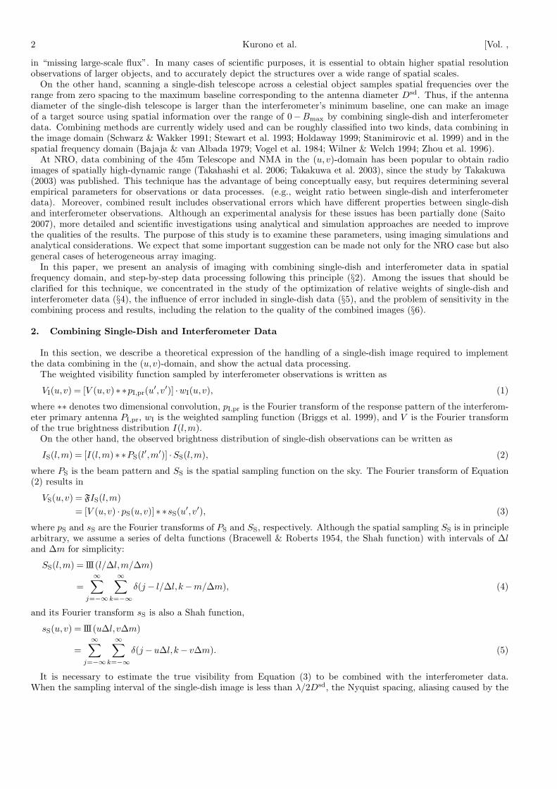
Figure 16-(a) shows the fraction of total flux recovered as a function of the noise level of the single-dish image,∆T sd. The fraction of recovered flux is almost unity is kept in respect of ∆T sd, and it is understood not to depend onthe quality of the single-dish image combined. Figure 16-(b) to -(d) show the image fidelity median, the (u,v)-fidelitymedian in the complement region (≤ 2.89kλ), and in the outer region (> 2.89kλ). Image fidelity and (u,v)-fidelity inthe outer region depends weakly on the quality of single-dish data, slowly decreasing with noise level of the single-dishimage. In contrast, the (u,v)-fidelity in the complement region strongly depends on the noise level of the single-dishimage. As the noise level of the single-dish image increases to ∆T sd ∼ 1K, this (u,v)-fidelity rapidly decreases. Whenthis noise level ∆T sd ∼ 1K is exceeded, the decrease rate of the (u, v)-fidelity in the complement region becomesgradual. In addition, ∆T sd ∼ 1K (SNRsd ∼ 20) corresponds to the boundary beyond which large-scale errors begin toappear in the difference images (figure 15).

Furthermore, we assessed the quality of the combined images by taking the autocorrelation (AC) of the differenceimage. We define RAC as the residual distribution by subtracting the AC of CLEAN beam, ACCB, from the AC ofthe difference image, ACDI:

RAC(i, j) ≡ ACDI(i, j)−ACCB(i, j). (36)

If the difference image includes only ideal uncorrelated noise, the AC should be equal to the AC of the CLEAN beamwhose peak value is equal to the variance of the image. However, if there are errors with some coherent structures, theAC will also have some structure other than beam-like, or its width will be extended. Two examples of RAC are shownon the right side of figure 16. Extended structures or patterns are emphasized in the cases of poor signal-to-noiseratio single-dish data, which indicates that the difference image includes a coherent structure rather than noise-likecomponents. Specifically, it can be said that the difference image with the smallest variance of RAC is the mostnoise-like. The rms level of RAC as a function of noise level of the single-dish image is shown on the left side of figure17. The RAC rms obviously increases as the signal-to-noise ratio of the single-dish image becomes worse, especiallybeyond ∆T sd ∼ 1K.

These results show that the combined image is dramatically degraded when the noise level of single-dish imageexceeds ∆T sd ∼ 1K (SNRsd ∼ 20). Thus, observing times of the single-dish that achieve the noise levels of ∆T sd ∼ 1Kare needed in this case. If the observation time is longer than that, the quality of the combined image does notimprove.


6.4. Sensitivity Balance between the Interferometer and Single-Dish Data

In the previous section, it was shown that there is a threshold of the noise level of the single-dish image not todegrade the combined image. This result is consistent with the argument by Vogel et al. (1984) that the signal-to-noiseratio of the visibilities derived from the single-dish data should be equal to that sampled by the interferometer not todegrade the combined image.

If density distribution of (u,v)-sampling points in the interferometer observation is written as nintvis(u,v), the total

number of visibilities is given as

N intvis =

∫nint

vis(u,v)dudv. (37)

When the visibility data is averaged over a (u, v)-cell which has the area of ∆u∆v, the integration time for this(u,v)-cell is given by tint

cell(u,v) = nintvis(u,v) ·∆u∆v · tint

vis, and the rms noise level in a (u,v)-cell by

∆Sintcell(u,v) =

√2kBT int

sys

ηinta ηcAint

√tintcell(u,v)∆ν

= ∆Sintvis ·

[nint

vis(u,v)∆u∆v]−1/2

. (38)

Therefore, the condition that the noise of the single-dish visibility ˆσsd′′ and that of interferometer visibility ∆Sintcell

are identical at a (u,v)-distance of b0 can be written as

σsd′′2

(b0) = σsd2 π

N2ln2

(Dsd

Dint

)2

exp(

π2θ2S

2ln2b20

)= ∆Sint

cell

2(b0), (39)

using Equation (24).The rms noise level of our simulated NMA data in §6.3 is ∆Sint

im = 0.11Jybeam−1, and estimated noise level in a(u,v)-cell is ∼ 2.9Jy when the (u,v)-cell ∆u∆v is set to 1kλ23. The derived rms noise level of the single-dish image is0.93K (SNRsd ∼ 20) from Equation (39). A noise level of ∆T sd ∼ 0.93K is consistent with the boundary beyond whichthe combined image is degraded, ∆T sd ∼ 1K. The noise distribution of the single-dish and the interferometer datain this case is shown in figure 18. Consequently, the suggestion by Vogel et al. (1984) is proven to be quantitativelycorrect.

From Equation (39), we obtain the integration time of the single-dish observation per pointing,

tsd =π3

29 ln2

(ηcη

inta

ηswηmbfs

)2(

T sdsys

T intsys

)2Aint

Asd

×exp(

π2θ2S

2ln2b20

)·nint

vis(b0)∆u∆v · tintvis. (40)

The total integration time is estimated by multiplying tsd by the number of total grid points, tsdN . If we assumea situation when the (u,v)-track is represented by an ensemble of concentric circles, the density distribution of the(u,v)-sampling points is inversely proportional to the (u,v)-distance, simply, nint

vis(u,v) ∝ 1/b. Thus, from Equation(35), we obtain

nintvis(u,v) = nint

vis(b)

=N int

vis

2π(bmax − bmin)· 1b. (41)

The total number of interferometer visibility data N intvis can be written as N int

vis = tinttrackNcorr/tint

vis, where tinttrack and Ncorr

are on source tracking time and the number of correlations, respectively. Thus, Equation (39) can be rewritten as:

tsd ≈ π

210 ln2

(ηcη

inta

ηswηmbfs

)2(

T sdsys

T intsys

)21D2

×exp(

π2

2ln21D2

)1

B− 1Ncorr · tint

track, (42)

3 In the imaging process, the image size is usually set to twice or more of the primary beam; the (u,v)-cell size of ∼ 1kλ2 is appropriate(corresponding to ∼ 200arcsec).


where we set b0 to the edge of (u, v)-hole, b0 = bmin = Dint/λ and the beam size of the single-dish observations toθS ≈ λ/Dsd. In the derivation of Equation (42), we assumed the simple model of nint

vis(u,v) ∝ 1/b of Equation (41) inwhich noise level in the (u,v)-cell should be ∆Sint

cell ∝ b1/2, and the (u,v)-cell corresponding to twice the primary beamsize of the synthesis image, ∆u∆v ≈ (2λ/Dint)−2. The expected noise distribution from this model is also shown infigure 18; it is found that this model is quite valid for the antenna configurations of the NMA. In addition, using theparameters in table 1, we can roughly estimate as tsd ∼ 1.2× 10−4 tint

track. Consequently, the total integration time of45m Telescope (to obtain an image with a size of four times as large as the primary beam width with the Nyquist gridspacings) is estimated to be ∼ 20% of total observing time for target source with the NMA.

7. Summary

We have studied the combining technique of single-dish data and interferometer data by simulations and analyticalconsiderations. In this report, we discussed the following issues: (1) weights applied to the visibilities estimated fromsingle-dish data and those obtained with interferometer, (2) deterioration of single-dish data due to pointing accuracy,(3) optimization of sensitivity, that is, determination of relative observation times of single-dish and interferometer.

The main results of our study for general issues are as follows:1. It is essential that there is no bias toward positive or negative in the difference between the combined synthesized

beam and the CLEAN beam in order to obtain high quality combined images. One should apply adequate weights tothe visibility data of single-dish and interferometer so that the mean of the difference between the synthesized beamand the CLEAN beam is close to zero when combining the data.

2. For a well scanned single-dish image, we obtained a relation between the rms of pointing error in the single-dishobservations and (u,v)-range that can be effectively used for the data combining. If we require an amplitude accuracywithin εpe,blur, the relationship between the rms of the pointing error σpe and the effective baseline length beff is givenby σpebeff ≤

√− ln(1− εpe,blur)/(2π2).

3. The error in single-dish deconvolution caused by the difference of beam shape from an ideal Gaussian is smallwhen using a single-dish with larger aperture. If we require an amplitude error better than 10% caused by theuncertainty of the beam shape, the diameter of the single-dish should be at least 1.7 times larger than the minimumbaseline of the interferometer.

4. We derived an analytical expression of the contribution of single-dish noise in the combining process, and derivedthe noise variance in the combined image. We confirmed the consistency with the results with noise-added simulations.

5. When the noise of the single-dish image is larger than a threshold level, a large-scale error distribution appearsin the combined image. From quantitative analysis, it is shown that the noise of the visibility obtained from thesingle-dish image has to be equal to that of interferometer data not to degrade the combined image. From this, wederived the useful expressions that estimate the adequate single-dish observing time.

Although we assumed to use 45m Telescope and NMA, our considerations can be used in a general discussion ofheterogeneous array imaging. In particular, this technique is the most basic and essential portion of the role of theAtacama Compact Array (ACA) in the Atacama Large Millimeter/Submillimeter Array (ALMA) observing system inthe near future, in order to improve the quality of obtained image dramatically.

The authors thank S. Takakuwa and H. Saito for valuable discussions. We are also grateful to the staff of theNobeyama Radio Observatory and the ALMA-J Project Office for continuing interest, encouragement, and usefulcomments. Y. K. would like to thank B. Vila-Vilaro for helpful discussions.

References

Bajaja, E., & van Albada, G. D. 1979, A&A, 75, 251Bracewell, R. N., & Roberts, J. A. 1954, Australian Journal of

Physics, 7, 615Briggs, D. S., Schwab, F. R., & Sramek, R. A. 1999, Synthesis

Imaging in Radio Astronomy II, 180, 127Christiansen, W. N., & Hogbom, J. A. 1985, Radio Telescopes

(Cambridge: Cambridge Univ. Press)Cornwell, T., Braun, R., & Briggs, D. S. 1999, Synthesis

Imaging in Radio Astronomy II, 180, 151Holdaway, M. A. 1999, Synthesis Imaging in Radio Astronomy

II, 180, 401Hogbom, J. A. 1974, A&AS, 15, 417Narayan, R., & Nityananda, R. 1986, ARA&A, 24, 127Pety, J., Gueth, F., & Guilloteau, S. 2001, ALMA Memo 398Saito, H. 2007, NRO Technical Report, No.69

Sault, R. J., Teuben, P. J., & Wright, M. C. H. 1995,Astronomical Data Analysis Software and Systems IV, 77,433

Schwarz, U. J. 1984, Indirect Imaging. Measurement andProcessing for Indirect Imaging, 255

Schwarz, U. J., & Wakker, B. P. 1991, IAU Colloq. 131: RadioInterferometry. Theory, Techniques, and Applications, 19,188

Stanimirovic, S., Staveley-Smith, L., Dickey, J. M., Sault,R. J., & Snowden, S. L. 1999, MNRAS, 302, 417

Steer, D. G., Dewdney, P. E., & Ito, M. R. 1984, A&A, 137,159

Stewart, R. T., Caswell, J. L., Haynes, R. F., & Nelson, G. J.1993, MNRAS, 261, 593

Takakuwa, S., Kamazaki, T., Saito, M., & Hirano, N. 2003,ApJ, 584, 818

Takakuwa, S. 2003, NRO Technical Report, No.65


Cross−calibration

45m visibility data

Combined imaging

NMA raw visibility data

Flux conversion to Jy/pixel

Deconvolution

(Wiener filtering with gaussian func.)

Multiply NMA primary beam

Make 45m visibilities in overlap region

Make 45m visibilities in complement region

Calibration

Make 45m map cube

45m raw spectral data

45m map cube data

Calibration

Fig. 1. Flow of the data combining process.

Takahashi, S., Saito, M., Takakuwa, S., & Kawabe, R. 2006,ApJ, 651, 933

Thompson, A. R., Moran, J. M., & Swenson, G. W., Jr.2001, Interferometry and synthesis in radio astronomy, 2ndedition (New York: John Wiley & Sons)

Vogel, S. N., Wright, M. C. H., Plambeck, R. L., & Welch,W. J. 1984, ApJ, 283, 655

Wilner, D. J., & Welch, W. J. 1994, ApJ, 427, 898Zhou, S., Evans, N. J., II, & Wang, Y. 1996, ApJ, 466, 296


Fig. 2. Left: (u,v)-coverage after the combining process. Green and blue plots show the NMA data and that in the overlap region ofthe 45m Telescope and the NMA, respectively. Red shows the visibilities generated from the 45m Telescope data in the complementregion. The declination is 30. Right: An example of simulated visibilities obtained with the NMA and generated from the 45mTelescope data through the combining process, for the case of no observational error and noise-free (§4.2). The source model isspherical.

Table 1. Simulation parameters

Common parametersResolution 0′′.25× 0′′.25, 0′′.5× 0′′.5a

Size 2048pix× 2048pixObserving frequency ν 86.75433GHzFrequency width ∆ν 31.25kHz

Interferometer observations (NMA)Antenna diameter Dint 10mNumber of element antennas Nant 6-elementsNumber of baselines Ncorr 15-baselinesPrimary beam 79′′ GaussianAntenna configuration D + C configurationsPhysical baseline range 13− 163mTracking time tint

track −4 to 4hrIntegration time per visibility tint

vis 16secSystem temperature T int

sys 400KAperture efficiency ηint

a 0.65Correlator efficiency ηc 0.85

Single-dish observations (45m Telescope)Antenna diameter Dsd 45mBeam 18′′.5 Gaussian, Non-Gaussianb

Observed region L2 ∼ 320′′ × 320′′Grid intervals ∆l×∆m 7′′.75× 7′′.75System temperature T sd

sys 250KSwitching efficiency ηsw 1/

√2

a §5.2b see table 2 for §5.2


Elliptical ModelSpherical Model

Fig. 3. The “spherical” model source (left) and the “elliptical” model source (right) used in our simulations. The sphericalmodel is a combination of three circular Gaussian patterns with FWHMs of 60′′, 10′′, and 3′′, respectively, and has a total fluxof 370.9Jy. The elliptical model is a combination of three elliptical Gaussian patterns with FWHMs of 90′′ × 30′′, 15′′ × 5′′, and4′′.5 × 1′′.5, respectively, all at position angles of 45. This model source has a total flux of 278.175Jy. Upper: The intensitydistribution of the model sources. Resolutions of these images are 0′′.25, and intensity units in Jypixel−1. Lower: Profiles cut alongDEC offset = 0arcsec for the spherical model, and along major (solid) and minor (dashed) axis for the elliptical model.

Table 2. Parameters of the simulated single-dish beams in Fig. 11

quadripod support tripod supportFWHM 19′′.94 19′′.59First sidelobe level −16.2dB −20.5dBAperture efficiency ηa 0.66 0.69Main beam efficiency ηmb 0.93 0.94JyK−1 2.64 2.50


Table 3. Notation of noise analysis in §6.1

Notation Description EquationDsd, Dint antena diameter of a single-dish telescope and an interferometer (23)

λ observation wavelength . . .L image size of a single-dish image . . .N number of pixel points in a single-dish image . . .θS FWHM of single-dish beam (19)pi pixel value of Fourier transform of interferometer primary beam (20)

θI,pr FWHM of interferometer primary beam . . .ˆθI,pr FWHM of Fourier transform of interferometer primary beam (22)

∆Ssd noise equivalent flux density (NEFD) of single-dish observations (25)Ωpix solid angle of a pixel (25)ηmb main beam efficiency of single-dish observations (25)ηsda aperture efficiency of single-dish observations (25)fs source filling factor (25)

Asd physical collecting area of single-dish aperture . . .∆T sd rms noise level in a single-dish image in K (9)∆Ssd

pix rms noise level in a single-dish image in Jypixel−1 (25)εsdn pixel noise in a single-dish image (14)εsd

m pixel noise in a Fourier transform of single-dish image (complex) (14)

εsdm

′pixel noise in a Fourier transform of single-dish image after deconvo-lution (complex)

(20)

εsdm

′′pixel noise in a Fourier transform of single-dish image after deconvo-lution and primary beam multiplication (complex)

(20)

σsd maximum likelihood of single-dish noise in the (u,v)-domain (16)

σsd′(b) maximum likelihood of single-dish noise in the (u, v)-domain after

deconvolution (a function of (u,v)-distance)(19)

σsd′′(b) maximum likelihood of single-dish noise in the (u, v)-domain after

deconvolution and primary beam multiplication (a function of (u,v)-distance)

(24)

Table 4. Notation of noise analysis in §6.2

Notation Description EquationV constant real-valued visibility of a point source (27)

N intvis number of interferometer visibility data (27)

N sdvis number of single-dish visibility data (27)

N intvis total number of visibility data (27)

wn weight applied to visibility data (27)εR real part of complex noise (27)I0 intensity estimate in a combined image (29)σ2

c variance of estimated intensity in a combined image (29)Cdep number of dependent noise combinations for single-dish data (30)

nsddep,cell number of dependent noise samples for single-dish data (32)∆Sint

vis rms noise level per interferometer visibility (34)∆Sint

im rms noise level in an interferometer synthesized image (35)B ratio of maximum to minimum baseline of interferometer observations (35)D ratio of single-dish to interferometer antenna diameter (35)

∆Scomb rms noise level of a combined image . . .


Fig. 4. The lower panels show simulated synthesized beams of the combined data (45m Telescope + NMA). The upper panelshows slices of the synthesized beams along declination at R.A. offset = 0arcsec. The (u,v)-range into which the 45m Telescope datais added is ≤ 2.89kλ, and the NMA data is obtained with the (u,v)-coverage of D- and C-configurations. The declination of thetracking center is 30, and the averaged density ratios are β = dsd/dint = 1/2, 5, 20. Contour levels are ±0.1, 0.2, 0.3, 0.4, 0.5.


Fig. 5. Left: Major and minor axes of the combined synthesized beams as a function of the averaged (u,v) weight ratio, β. Right:The mean of the difference image between the combined synthesized beam and the CLEAN beam as a function of β.


Fig. 6. Images of noise-free combine simulations. Combined dirty images (left), CLEANed images (center), and difference imagesbetween the CLEANed images and the model images multiplied by the primary beam and convolved with the CLEAN beams (right).The averaged density ratios are β = dsd/dint = 1/2 (top row), 5 (middle row), and 20 (bottom row). The “spherical” model at adeclination of 30 was used. The difference images are shown in percentage of the peak of the model image.


Fig. 7. Image fidelity median (a), (u,v)-fidelity median for the complement region ((u,v)-range of ≤ 2.89kλ) (b) and outer region(> 2.89kλ) (c), and fraction of total flux recovered (d) as a function of β. The lines indicate different source declinations of 50,30, 10, and −10 (left) and observed model sources; the spherical model of ×1/2 size, ×2 size, and the elliptical model (right).The shadowed range of β where the mean of the beam difference crosses zero (Figure 5).


Fig. 8. Single-dish images with random pointing errors (left) of a single map and average of 10 maps, combined dirty images(center), and difference images between the data with and without the pointing errors (right). The source is the “spherical” model.Pointing errors are 3′′ (top), 6′′ (middle), and 9′′ (bottom) in rms. The averaged weight ratio applied to the visibility data is β = 5.

Fig. 9. Rms of the difference between the combined images with and without single-dish pointing errors. The error in total flux(after combine) as a function of pointing error is also indicated.


Fig. 10. The distributions of visibility amplitude in the case of combine with single-dish pointing errors The single-dish images area single map and average of 10 maps. The model source is spherical. The pointing errors included in the single-dish observations are3′′ (left), 6′′ (center), and 9′′ (right) rms. These plots show the data of model sources (black), observed by the interferometer (green),and generated from the single-dish image (red and blue). The visibility data shown in blue are generated from the single-dish imagesin the overlap region. The ratios of the visibility amplitudes generated from the single-dish data to the model data are shown in thelower panels. The dotted lines indicate the distributions of expected amplitude ratios (see text).


Fig. 11. Simulated single-dish beam patterns. Assumed illumination distributions of the aperture (left) and beam patterns (right),for sub-reflector support types, tripod (upper) and quadripod (lower).


Fig. 12. Upper: The response patterns in the (u, v)-domain of the simulated model beams (dots), and Gaussians of the sameFWHM as the model beams (dotted lines). Lower: Sensitivity ratio of the model beams to the Gaussian patterns.


Fig. 13. The noise distribution in the (u,v)-domain of the simulated single-dish data of the original (black), and that of deconvolvedand multiplied by the primary beam in the complement region (red) and the overlap region (blue). The rms noise level of the originalsingle-dish image is 0.1K. Dots and squares indicate the raw data and averages with (u,v) width of 1kλ, respectively. The theoretical

expectationp

π/2 ˆσsd′′(b) is shown as a dashed line.


Fig. 14. The rms noise level of the combined image as a function of (u,v)-weight ratio β and rms noise level of the single-dishdata. The left panel shows the simulation results (average results over 10 simulations) and the right panel shows the analyti-cal solution (Equation 35). The white line traces ∆Scomb = ∆Sint

im . The image sensitivity of the interferometer data alone is

∆Sintim = 0.11Jybeam−1.


Fig. 15. Images of combine simulations with thermal noise. The model source used is the “spherical”. Combined dirty images (left),restored images of SDI CLEAN (center), and difference images from the model (right), for the signal-to-noise ratios of single-dishdata of SNRsd ∼ 3,10,20,90,200,916. The averaged density ratio is β = 5.


Fig. 16. Fraction of total flux recovered (a), image fidelity median (b), (u,v)-fidelity median for the complement region ((u,v)-rangeof ≤ 2.89kλ) (c) and for outer region (> 2.89kλ) (d) as a function of the noise level of the single-dish image ∆T sd. The results arethe average over 10 simulations. The averaged weight ratio is β = 5.


Fig. 17. Right: The residuals of the subtraction of the autocorrelation of CLEAN beam from the autocorrelation of the differenceimage (RAC). The signal-to-noise ratio of the single-dish images combined is SNRsd ∼ 3 (a) and ∼ 1820 (b), respectively. Left: Rmslevel of RAC as a function of the rms noise level of the single-dish data, ∆T sd (average results over 10 simulations).

Fig. 18. Distribution of the simulated noise amplitude as a function of (u,v)-distance. Left: Visibility of interferometer observationsand for the single-dish data on 1kλ2 cell. The rms noise level of the original single-dish image is 0.93K. Right: Mean amplitudeof the averaged noise visibility over the (u,v)-cell shown in the left panel. For comparison, the cases of single-dish rms noise levelsof 0.19K and 4.65K are also shown. The dashed line indicates a model of interferometer noise function, ∆Sint

cell ∝ b1/2, by a simple

assumption that density of measured points in the (u,v)-domain is inversely proportional to the (u,v)-distance, nintvis(u,v) ∝ 1/b.

a study of combining technique of single-dish and ...lib_pub/html/report/data/tno73.pdf ·...

Documents