A Structural Econometric Analysis of the Informal Sector

Heterogeneity1

Pierre Nguimkeu

Department of Economics; Andrew Young School of Policy Studies;Georgia State University;

PO Box 3992 Atlanta, GA 30302-3992, USA;Email: nnguimkeu@gsu.edu

Abstract

Understanding the informal sector - that represents about 60− 90% of ur-ban employment in developing countries - has a significant importance for anystrategy and policy interventions aiming to alleviate poverty and improve wel-fare. I formulate and estimate a model of entrepreneurial choice to address theheterogeneity in occupations and earnings observed within the informal sec-tor. I test the implications of the model with reduced form and nonparametrictechniques, and use a structural econometric approach to empirically identifyoccupational patterns and earnings using data from the Cameroon informalsector. The empirical validity of the structural estimates is tested and theestimated model is used in a counterfactual policy simulation to show how mi-crofinance can strengthen the efficiency of the informal sector and substantiallyimprove its earning potential.

Keywords: Occupational choice; Financial constraints; Maximum likeli-hood estimation; Informal economy; Specication analysis.

JEL Classification: O12, O17, C51, C52, C54.

1I gratefully acknowledge financial support from the Social Science and Humanities ResearchCouncil of Canada (SSHRC). I thank the National Institute of Statistics of Cameroon for makingthe data available to me for this study. Comments from Emmanuelle Auriol, Jean-Paul Azamand participants of the the CEA and WEAI conferences are gratefully acknowledged. I am muchindebted to Pascal Lavergne and Alexander Karaivanov for intensive discussions and advices.

1 Introduction

In developing countries, the informal sector has an overwhelming importance for atleast three reasons. First, it is a response to poverty and unemployment; informalentrepreneurs drive job formation through small-business creation.1 Second, it isconsidered an incubator for business potential and a stepping stone for accessibilityand graduation to the formal economy (ILO 2002). Third, it absorbs the majorityof the workforce; about 60− 90% of the overall employment is in the informal sector(UN-Habitat 2006, ILO 2009). However, in spite of involving so much workforce theinformal sector produces only 10− 40% of the gross national product, essentially be-cause informal subsistence activities characterized by labor-intensive and low-incomegenerating businesses predominate this economy. In fact, a typical feature of the in-formal sector which is increasingly referred to in the literature as “upper” and “lower”tiers segmentation, is that it includes both urban poor people, who depend on in-formal subsistence activities for their livelihood, as well as relatively higher-incomepeople most of whom are micro-entrepreneurs running small or medium size enter-prises that use capital and hire labor (Fields 1990). Understanding this heterogeneitythat characterizes the informal sector therefore has significant implications for anystrategy and policy interventions aiming to alleviate poverty and improve economicwelfare.

This paper contributes to this objective by providing an econometric analysisof the heterogeneity observed in the informal sector. I formulate and estimate astructural model of occupational choice where informal sector agents choose be-tween subsistence activity and entrepreneurship, and their decision-making processdepends on their entrepreneurial skills as well as their access to credit. I test the im-plications of the model with reduced form and nonparametric techniques, and use astructural econometric approach to empirically identify the relationship among skills,initial wealth distribution, and occupational patterns and earnings using data fromthe Cameroon informal sector. The empirical validity of the structural estimates istested using the Lavergne and Nguimkeu (2011) specification test, and the estimatedmodel is used in a counterfactual policy simulation to show how microfinance canstrengthen the efficiency of the informal sector and substantially improve its earningpotential.

The model used to approximate individual behavior is an extension of a widely

1More than 90% of new jobs created between 1990 and 1994 in Africa were in the informal sector(Kuchta-Helbling 2000).

1

used empirical specification that is featured in Evans & Jovanovic (1989). Eachagent compares the expected gain he or she would obtain from subsistence activityto the expected profit accruing from running a firm. An individual in the subsis-tence activity receives a fixed income while an entrepreneur establishes a firm withcapital investment and realizes profit from a decreasing-returns-to-scale productiontechnology. Entrepreneurship promises higher expected earnings, but requires higherskills and higher starting capital that can be supplemented by borrowing. However,because of credit market imperfection, borrowing is exogenously limited to a fixedmultiple of initial asset. Initial wealth therefore plays the role of collateral and isrequired by financial institutions as a strategy to reduce default. Thus low-wealth en-trepreneurs may be constrained in their investment and some potential entrepreneursmay be unable to borrow to finance their projects in spite of having a good en-trepreneurial idea. The main implication of the model is that entrepreneurial choiceand entrepreneurial earnings are positively related not only to skills but also to ini-tial wealth. In order words, if profitable entrepreneurial activities (entrepreneurship)require getting a certain level of initial wealth to use as collateral in the capital mar-ket, poorly endowed individuals will not engage in such activities. They will ratherremain in subsistence activities that require no capital, so that, the higher the shareof initially poor people in the economy, the bigger the size of the subsistence segment.

The main focus of this work is to use data from Cameroon to address the het-erogeneity observed in the informal sector whose stylized facts are comparable tothose produced by the theoretical model, and then use the estimated model to for-mulate and perform welfare analysis that allow to quantify the impact of relevantpolicies. The structural parameters of the model are estimated using maximum like-lihood estimation technique. The likelihood function is constructed by matchingthe expected probability of becoming a micro-entrepreneur generated by the the-oretical model (expressed as a function of initial wealth and other individual andmarket characteristics) with the corresponding household occupational status ob-served in the data. The econometric analysis is performed for the whole sample, aswell as for various data stratifications including urban, rural and metropolitan areas.The model implications are also tested through reduced form estimation (includingProbit and Quantile regressions) that make use of multivariate controls as well asnon-parametric estimation that do not impose any a priori structure to the relation-ship among the variables. I use these techniques not only to check the robustness ofthe structural findings but also to examine to what extend other factors not featuredin the theoretical model may influence entrepreneurial choice. A validity check todetermine how close the specified model is to the data is also performed by applying

2

the Lavergne & Nguimkeu (2011) model specification test.

The empirical analysis uses data from a cross-sectional sample of householdsof Cameroon stemming from the 2005 National Survey on Employment and Infor-mal Sector (EESI). This survey is a two-phase nationwide operation conducted bythe National Institute of Statistics in partnership with the World Bank. The firstphase collects socio-demographic and employment data while the second phase in-terviews a representative subsample of informal production units identified duringthe first phase. The methodology of the EESI is therefore similar to that of Phases1 and 2 of the well known “1-2-3 surveys” in Central and West Africa. Only datafrom Phase 1 are used here. The estimation results reveal that more than 80% ofmicro-entrepreneurs are credit constrained and that these constraints are the mainsource of the differences in informal enterprises returns, which is consistent withprevious results in the literature. More interestingly, they reveal that credit con-straints also affect people’s occupational choices and explain the preponderance ofmassive subsistence activities characterized by low earnings that coexist with micro-enterprises. Education also appears to be a key determinant of occupational patternsand entrepreneurial earnings in the informal sector. This result has been already em-phasized in Nguetse (2009), who estimated returns to education in the Camerooninformal sector using this same dataset. These findings then suggest that appro-priate financing schemes can improve welfare by reducing the misallocation of skillsacross occupations and raising the earning potential of the informal sector. To con-firm this intuition, I use the structural estimates to perform a counterfactual policyexperiment that evaluates the impact of a micro-lending program using an approachsimilar to Buera et al. (2011). The results show that by allowing individuals toborrow up to three times the value of the average household wealth the proportionof micro-entrepreneurs can substantially increase by up to 9%, representing twice asmuch micro-entrepreneurs in the economy, while the average earnings of the overallinformal sector can increase by more than 30%. Moreover, they show that the het-erogeneity of returns among informal enterprises stemming from differences in levelsof starting capital can be considerably lowered.

Several other studies have addressed the heterogeneity observed in the informalsector and the related differences in occupations and earnings. A growing literatureargues that social norms and solidarity prevailing in Africa constitute a significanthandicap to micro-entrepreneurial investment (see Duflo et al 2009; Nillesen, Beek-man & Gato 2011), and a serious barrier to entrepreneurial choice (Alby, Auriol &Nguimkeu 2011; Grimm et al. 2010). However, the most widely documented con-

3

straints to informal entrepreneurship in Africa are lack of skills and initial capitalrequirements (Fields 1990; Cunningham & Maloney 2001). Following various the-oretical models of inequality and poverty traps that emphasize the role of wealthdistribution as an explanation of the coexistence of high and low returns in economicactivities (see Banerjee & Newman 1993, Piketty 1997, Aghion & Bolton 1997, Lloyd-Ellis & Bernardt 2000, Ghatak & Jiang 2002, Gine & Townsend 2004), skills andstarting capital requirements have been empirically posited by some authors as beingthe main sources of the segmentation observed in the informal sector. A noticeableempirical contribution in the Sub-Saharan Africa context is Grimm et al. (2010)who studied how entry costs and starting capital affect marginal returns to capitalin micro-enterprises. Using micro-enterprises data from West-African countries theyshow that different levels of starting capital can explain the observed heterogeneityin capital returns. Their findings, however, fit only entrepreneurial businesses andfail to identify the massive subsistence segment of informal activities characterizedby very low capital stocks and low returns that coexists with these micro-enterprisesin the informal sector.2 Moreover, their framework does not allow to test and quanti-tatively evaluate the implications and magnitude of policy strategies, as a structuralapproach would do. This paper is therefore a complementary work to Grimm et al.(2010) in these respects.

The rest of the paper is organized as follows. Section 2 describes a theoreticalmodel of occupational choice under imperfect credit markets and establishes the mainimplications for the informal sector. Data and reduced form results are presented inSection 3. Structural estimation of the theoretical model and specification analysisare performed in Section 4. Section 5 evaluates the impact of policy experiments,followed by concluding remarks in Section 6. Section 7 provides additional tables,figures and other technical details.

2 Model Description and Implications

In this section, I present a basic model that I estimate and use to evaluate and quan-tify the impact of economic policies toward the informal sector. The model is anextension of Evans & Jovanovic (1989). The economy is populated by a continuumof agents who are potential entrepreneurs and who differ in their skill θ and their

2In fact, Grimm et al. (2010) find extremely high marginal returns of more than 100% at verylow levels of capital, which is not consistent with data from subsistence activities in West Africa.

4

level of initial wealth endowment z.3 At the beginning of the period, agents choosetheir occupation: whether to work in subsistence activity or to start a small business(entrepreneurship/micro-entrepreneurship). Since entrepreneurship is costly, theiroccupation choices are based on their comparative advantage as entrepreneur ac-cording to their access to capital. Access to capital is however limited by their initialwealth through an exogenous collateral constraint because of imperfect enforceabil-ity of capital rental contracts. It is assumed that each household operate only oneproduction unit and devote their entire labor endowment to their activity. The unitfixed gross rate of capital rental is r.

2.1 Subsistence activity

Households working in the subsistence tier require no capital. They use no technologyso that their skill θ is irrelevant and their expected payoff takes the form

πS = µ, (1)

where µ is a productivity parameter, which is assumed constant along the subsistencesector.4 This formulation of the subsistence earning is consistent with the view ofTodaro (1997) who characterizes the subsistence sector as an “easy-entry tier withexcess capacity and competition driving income down to the average supply of laborof potential new entrants.”

Some examples of subsistence activities include street-vending (e.g., a peanutsstand or a fruit stand), unpaid family labour or unskilled labour with non-specificwork relations. Such activities require relatively low set-up costs and there is noskill requirement to such work. Street-vending licenses are easily procured. Locationrental fees are nominal. Paid employees are rare (Fields 1990).

2.2 Entrepreneurship

An entrepreneur with skill θ uses capital k to produce goods according to the tech-nology

y = θkαε (2)

3I will use the terms agents, individuals and households interchangeably. Likewise for the termsskill, talent, and ability.

4The fact that any skill that the individual may have is irrelevant in the subsistence sector is asimplification that later proved useful for the identification of the model when estimating.

5

where α ∈ (0, 1) is the elasticity of output with respect to capital. The term ε is aproductivity shock, independent from θ and z, with positive support, mean 1 andvariance σ2

ε . At the end of the period, the entrepreneur’s net income is given by

θkαε− rk

We assume, as in Evans & Jovanovic (1989), that households can borrow onlyup to some fixed multiple of their total wealth, λz, but no more.5 The maximumamount that can be invested in their entrepreneurial business is then equal to λz,with λ ≥ 1 (so that one can always self-finance).6

The entrepreneur’s optimal investment capital then solves for his expected profitmaximization problem

max {θkα − rk} , s.t. 0 ≤ k ≤ λz,

with an interior solution

k∗ =

(θα

r

)1/(1−α)

. (3)

This solution is feasible only if the entrepreneur is unconstrained. This means thatk∗(θ) is lower than λz. Specifically, entrepreneurs will be unconstrained if, for agiven z, their ability θ satisfy

θ ≤ r

α(λz)1−α ≡ θ(z) (4)

Equivalently, the unconstrained condition also means that for a given θ, their initialwealth z must satisfy

z ≥ 1

λ

(θα

r

)1/(1−α)

≡ z(θ) (5)

Equation (4) means that for a given level of wealth, entrepreneurs will be uncon-strained only if their ability is low enough. Thus, holding household wealth con-stant, borrowing constraints are more likely to bind for higher skilled households.

5Even in the case where collateral may not be explicitly required in an informal lending likein the rotating saving and credit associations (ROSCA), the level of wealthiness of the borrowerstill influences the maximum amount that lenders would be willing to release. Thus, the maximumcapital that individuals can borrow may still be seen as depending on their initial wealth.

6The assumption that k ≤ λz can also be micro-founded or endogenized. Indeed, with a simplemodel of limited liability under asymmetric information a la Banerjee & Newman (1993) it can beshown that the optimal amount that a financial institution would be willing to lend to a borroweris a proportion of the borrower’s initial wealth. This is shown in the Appendix 7.5.

6

As for Equation (5), it tells us that for a given level of talent, entrepreneurs areunconstrained only if their initial wealth is high enough. For a given ability level θ,constrained entrepreneurs are those with initial wealth below the critical thresholdz(θ). Or, equivalently, for a given initial wealth level z they are those with abilityhigher than θ(z). For these households, the maximization constraint will be bindingso that they will invest λz in their entrepreneurial business, even though they wouldlike to invest more (see Figure 1).

The household expected profit in entrepreneurship therefore takes the followingform

πE(z, θ) =

(1− α)θ1/(1−α)

(α

r

)α/(1−α)

if z ≥ z(θ)

θ(λz)α − λrz otherwise.

(6)

2.3 Implications

Since households know their skill θ and initial wealth level z before choosing an oc-cupation, they choose entrepreneurship only if their expected profit from doing soexceeds what they would get by staying in the subsistence. In other words, they be-come entrepreneur only if their comparative expected profit, π(z, θ) = πE(z, θ)−πS,is non-negative.

Given Equations (1) and (6) obtained above, an expression for π(z, θ) can bederived as follows :

π(z, θ) =

(1− α)θ1/(1−α)

(α

r

)α/(1−α)

− µ if z ≥ z(θ)

θ(λz)α − λrz − µ otherwise.

(7)

Clearly, the comparative gain function, π(z, θ), does not depend on the initial assetz when the latter is higher than the critical wealth threshold z. This means thatwealthier households decisions to start a business does not depend on their capacity toget starting capital once they have enough, but only on whether they have sufficientskills. For further analysis, I define the critical ability level

θ∗ =

(µ

1− α

)1−α(r

α

)α(8)

7

The quantity θ∗ is a cutoff talent level that determines whether a financially un-constrained household has the ability to start a firm. This cutoff does not dependon wealth.7 In principle, if there were no financial constraints, all households withtalent above this threshold should choose to become entrepreneur. But because ofimperfect credit markets, I instead have the following result.

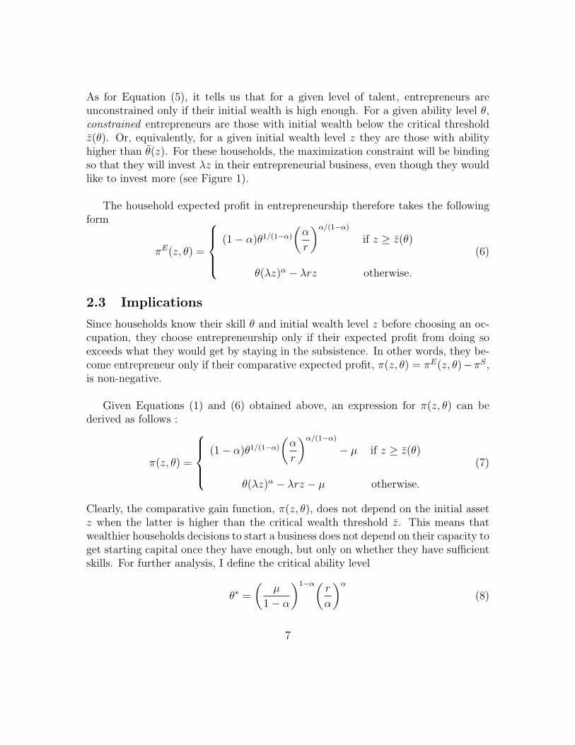
Proposition 1. Consider households with initial wealth z and ability θ.(i) For ability level θ, the function π(·, θ) defined in (7) is strictly increasing for allz ≤ z(θ), and constant for all z > z(θ).(ii) If θ ≤ θ∗, where θ∗ is defined in (8), then π(z, θ) ≤ 0 for all z.(iii) If θ > θ∗, there exists a critical wealth threshold z(θ) ∈ (0, z(θ)) such that,π(z, θ) < 0 ∀z < z(θ), and π(z, θ) > 0 ∀z > z(θ).

The behavior of the comparative gain function π(·, θ), as described in the aboveproposition, is illustrated in Figure 1.

Figure 1: Illustration of the comparative profit function

0 0.02 0.04 0.06 0.08 0.1!0.25

!0.2

!0.15

!0.1

!0.05

0

0.05

z0

!

!(z , ")

!(z , ") " > "!

!(z , ") " < "!

!z z" = "!

Student Version of MATLAB

Proposition 1 (i) says that at a given skill level, poorer household’s comparativegain from entrepreneurship increase with their initial wealth endowment, whereaswealthier households comparative gain from starting a business is invariant withtheir initial wealth. As for Proposition 1 (ii), it tells us that households with rela-tively low entrepreneurial ability get lower profit from starting a firm no matter theamount of wealth they have, so that they always choose subsistence activity. In con-trast, Proposition 1 (iii) emphasizes that having high skills is not enough to becomeentrepreneur. A minimum level of initial wealth is also required for this purpose.This result is driven by the existence of borrowing constraints in the credit market,which is captured in the model by the finite parameter λ. To analyze the behavior

7θ∗ is obtained by setting the upper right hand side of Equation (7) to zero and solving for θ.

8

of entrepreneurs who are indifferent between operating in either segments, we definethe critical level of wealth

z∗ =1

λ

µ

1− αα

r. (9)

The wealth level z∗ does not depend on households characteristics.8 For wealth levelsbelow z∗ the choice on the margin is between being a subsistence worker and startinga constrained firm. In this case, the household will start a firm if their ability satisfies

θ > (λz)−α[µ+ rλz]

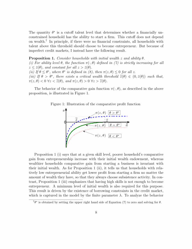
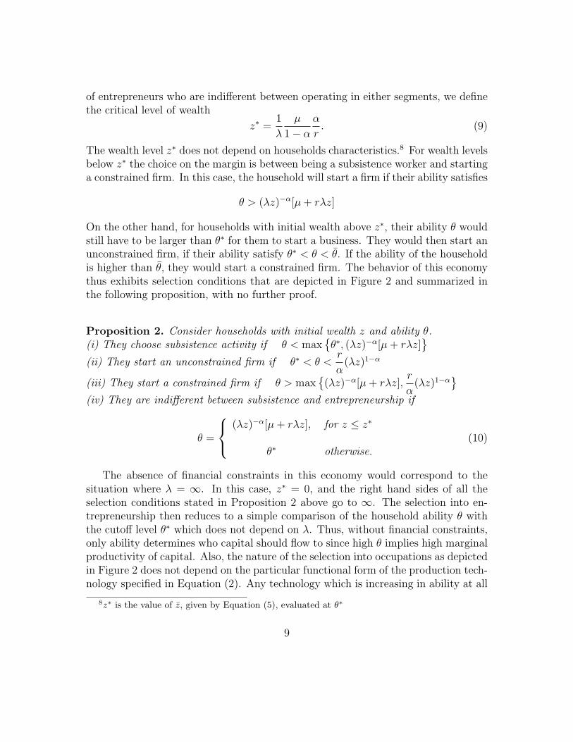
On the other hand, for households with initial wealth above z∗, their ability θ wouldstill have to be larger than θ∗ for them to start a business. They would then start anunconstrained firm, if their ability satisfy θ∗ < θ < θ. If the ability of the householdis higher than θ, they would start a constrained firm. The behavior of this economythus exhibits selection conditions that are depicted in Figure 2 and summarized inthe following proposition, with no further proof.

Proposition 2. Consider households with initial wealth z and ability θ.(i) They choose subsistence activity if θ < max

{θ∗, (λz)−α[µ+ rλz]

}

(ii) They start an unconstrained firm if θ∗ < θ <r

α(λz)1−α

(iii) They start a constrained firm if θ > max{

(λz)−α[µ+ rλz],r

α(λz)1−α}

(iv) They are indifferent between subsistence and entrepreneurship if

θ =

(λz)−α[µ+ rλz], for z ≤ z∗

θ∗ otherwise.(10)

The absence of financial constraints in this economy would correspond to thesituation where λ = ∞. In this case, z∗ = 0, and the right hand sides of all theselection conditions stated in Proposition 2 above go to ∞. The selection into en-trepreneurship then reduces to a simple comparison of the household ability θ withthe cutoff level θ∗ which does not depend on λ. Thus, without financial constraints,only ability determines who capital should flow to since high θ implies high marginalproductivity of capital. Also, the nature of the selection into occupations as depictedin Figure 2 does not depend on the particular functional form of the production tech-nology specified in Equation (2). Any technology which is increasing in ability at all

8z∗ is the value of z, given by Equation (5), evaluated at θ∗

9

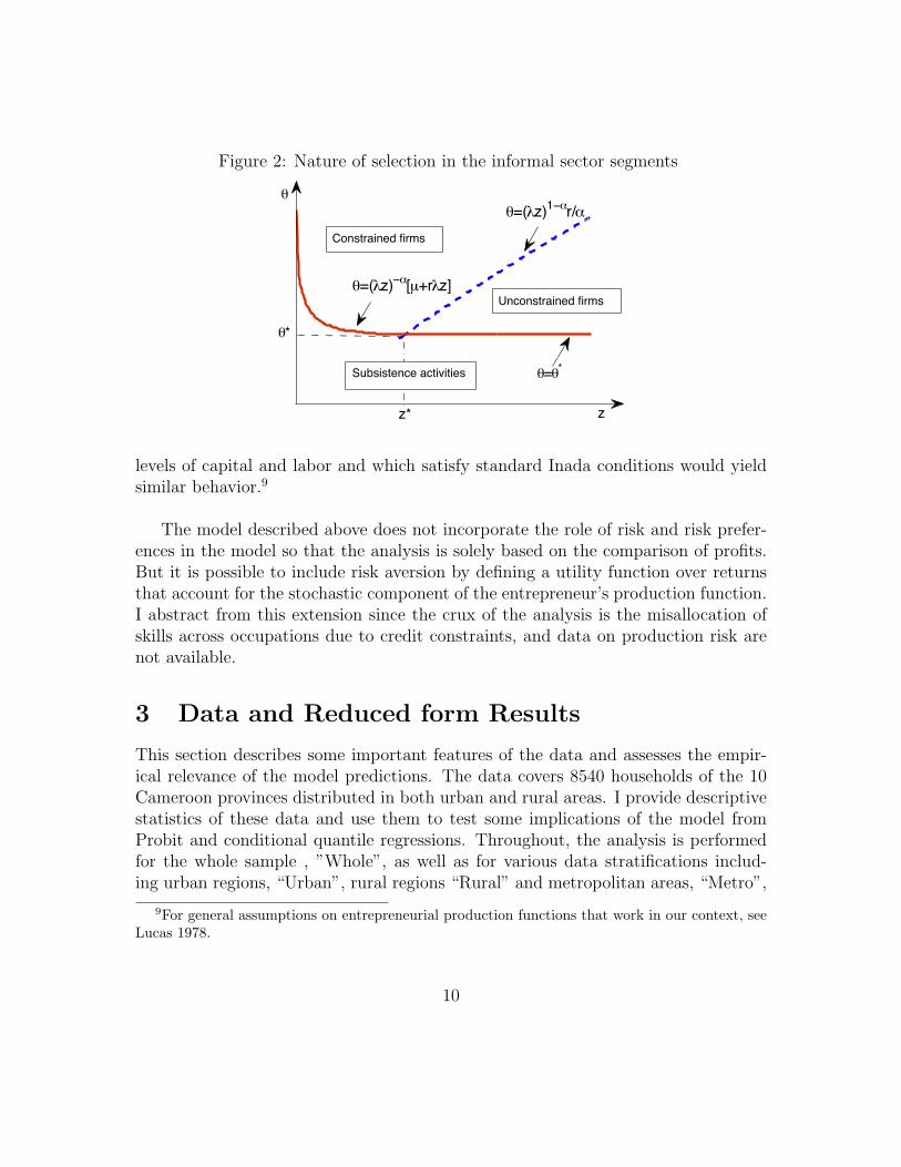
Figure 2: Nature of selection in the informal sector segments

0 0.01 0.02 0.03 0.04 0.050

0.1

0.2

0.3

0.4

0.5

0.6

0.7

0.8

0.9

1

!=!*

!=("z)1!#

r/#

!*

!

Constrained firms

Unconstrained firms

!=("z)!#

[µ+r"z]

z* z

Subsistence activities

Student Version of MATLAB

levels of capital and labor and which satisfy standard Inada conditions would yieldsimilar behavior.9

The model described above does not incorporate the role of risk and risk prefer-ences in the model so that the analysis is solely based on the comparison of profits.But it is possible to include risk aversion by defining a utility function over returnsthat account for the stochastic component of the entrepreneur’s production function.I abstract from this extension since the crux of the analysis is the misallocation ofskills across occupations due to credit constraints, and data on production risk arenot available.

3 Data and Reduced form Results

This section describes some important features of the data and assesses the empir-ical relevance of the model predictions. The data covers 8540 households of the 10Cameroon provinces distributed in both urban and rural areas. I provide descriptivestatistics of these data and use them to test some implications of the model fromProbit and conditional quantile regressions. Throughout, the analysis is performedfor the whole sample , ”Whole”, as well as for various data stratifications includ-ing urban regions, “Urban”, rural regions “Rural” and metropolitan areas, “Metro”,

9For general assumptions on entrepreneurial production functions that work in our context, seeLucas 1978.

10

formed by Douala and Yaounde, the two main cities that embed about 70% of theoverall economic activities of the country (see ECAM II Executive Report 2001).10

3.1 Descriptive statistics

The Cameroon National Survey of Employment and Informal Sector (EESI), fromwhich the data are drawn for this empirical investigation, defines informal enter-prises as “production units that do not have written formal accounts and/or are notregistered with the tax authorities.” Our sample contains 4337 households whoseactivities belong to the informal sector according to the above definition. The so-defined informal sector accounts for the vast majority of activities and employs about90% of the Cameroon workforce aged 15 and above. The employment shares of theinformal workforce are 60% for agricultural activities and 40% for non-agriculturalactivities. Households heads are either purely self-employed or employers with lessthan six employees.11 Most of the latter run only a single business and rely heavilyon family workers. Only 5% of the businesses hired and paid anyone from outsidetheir family and most of the activities surveyed were started less than 5 years earlierat the time of the survey. Non-agricultural activities are distributed along all thethree major sectors of the economy: manufacturing, commerce and services.

One interesting aspect of the EESI is that it provides information about bothhouseholds characteristics and the characteristics of the micro-enterprises that theypossibly run. It is thus an overlap of both household and enterprises surveys, whichmakes the dataset a comprehensive one that is useful to carry out extensive analysisabout households, associated firms and interactions. However, these data do notcontain a variable that reports household’s ex-ante total wealth, a key componentto our analysis. To deal with this lack of information, I construct an aggregate in-dex that represents the total wealth index of the household. This aggregate indexis created by a Principal Component Analysis from some of the household belong-ings reported in the questionnaires. Because the analysis requires that this indexbe representative of the initial wealth of the household, that is, their wealth priorto starting their current activity, only items that were acquired prior starting theiractivity are accounted for in the computation.12 A detailed description of the wealth

10ECAM II : Second Cameroon Household Survey administered by the National Institute ofStatistics in 2001; available at www.statistics-cameroon.org.

11Almost 90% of informal jobs come from business with generally less than 6 workers, mostlyunpaid family aids

12Although the survey is not dynamic, there are many retrospective questions that can be used

11

index can be found in Appendix 7.2.

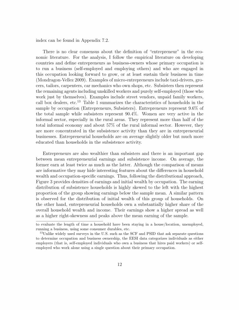
There is no clear consensus about the definition of “entrepreneur” in the eco-nomic literature. For the analysis, I follow the empirical literature on developingcountries and define entrepreneurs as business-owners whose primary occupation isto run a business (self-employed and employing others) and who are engaged inthis occupation looking forward to grow, or at least sustain their business in time(Mondragon-Vellez 2009). Examples of micro-entrepreneurs include taxi-drivers, gro-cers, tailors, carpenters, car mechanics who own shops, etc. Subsisters then representthe remaining agents including unskilled workers and purely self-employed (those whowork just by themselves). Examples include street vendors, unpaid family workers,call box dealers, etc.13 Table 1 summarizes the characteristics of households in thesample by occupation (Entrepreneurs, Subsisters). Entrepreneurs represent 9.6% ofthe total sample while subsisters represent 90.4%. Women are very active in theinformal sector, especially in the rural areas. They represent more than half of thetotal informal economy and about 57% of the rural informal sector. However, theyare more concentrated in the subsistence activity than they are in entrepreneurialbusinesses. Entrepreneurial households are on average slightly older but much moreeducated than households in the subsistence activity.

Entrepreneurs are also wealthier than subsisters and there is an important gapbetween mean entrepreneurial earnings and subsistence income. On average, theformer earn at least twice as much as the latter. Although the comparison of meansare informative they may hide interesting features about the differences in householdwealth and occupation-specific earnings. Thus, following the distributional approach,Figure 3 provides densities of earnings and initial wealth by occupation. The earningdistribution of subsistence households is highly skewed to the left with the highestproportion of the group showing earnings below the sample mean. A similar patternis observed for the distribution of initial wealth of this group of households. Onthe other hand, entrepreneurial households own a substantially higher share of theoverall household wealth and income. Their earnings show a higher spread as wellas a higher right-skewness and peaks above the mean earning of the sample.

to evaluate the length of time a household have been staying in a house/location, unemployed,running a business, using some consumer durables, etc.

13Unlike widely used surveys in the U.S. such as the SCF and PSID that ask separate questionsto determine occupation and business ownership, the EESI data categorizes individuals as eitheremployers (that is, self-employed individuals who own a business that hires paid workers) or self-employed who work alone using a single question about their primary occupation.

12

Table 1: Household Characteristics by occupation

Characteristics Whole Rural Urban Metro

Entr Subs Entr Subs Entr Subs Entr SubsNum. of obs. 424 3913 98 1270 326 2643 195 1299% of sample 9.4% 90.6% 7.3% 92.7% 10.5% 89.5% 12.9% 87.1%

% of women 6.4% 93.6% 4.7% 95.3% 7.4% 92.6% 9.3% 90.7%

Av. household size 6.1 5.8 6.3 5.7 6.2 6.0 5.7 4.8

Av. age of head 37.3 35.2 38.0 35.8 37.1 34.9 36.6 35.4Years of schooling

0-5 years 30.3% 45.1% 43.8% 57.8% 25.1% 37.9% 15.7% 24.8%6-10 years 49.4% 44.7% 43.0% 36.6% 51.8% 49.4% 53.0% 58.0%

11+ years 20.3% 10.2% 13.3% 5.6% 23.4% 12.8% 31.3% 17.2%

Av. income* 71.88 35.16 54.99 30.05 78.25 38.04 90.10 43.67Av. wealth index 7.30 3.08 3.77 2.09 7.74 3.69 8.37 4.34

*In thousands of local currency (CFA); 1, 000 CFA ∼ $2 US

Figure 3: Wealth (left) and Earnings (right) Distributions by Occupation

0 2 4 6 8 10 12 14 16 18 200

0.05

0.1

0.15

0.2

0.25

Entrepreneurs

Subsisters

Student Version of MATLAB

0 20 40 60 80 100 120 140 160 180 2000

0.005

0.01

0.015

0.02

0.025

0.03

0.035

Entrepreneurs

Subsisters

Student Version of MATLAB

There are very few options available through which entrepreneurial activities arefunded. Approximately 90% of the total initial business investment come from per-sonal savings, gifts from family and relatives, and inheritance. Loans represent theremaining 10% and come either from commercial banks or Microfinance institutions,from family or friends, and from ROSCAs (rotating saving and credit associations).Barriers hindering informal entrepreneurs from getting adequate access to credit arenumerous. The main reasons reported by the respondents were high interest rates

13

imposed by financial institutions and high collateral requirements. Both these areconsistent with the presence of financial market imperfections (asymmetric informa-tion, limited enforcement, etc.). Among the respondents, 40% acknowleged the needto get better access to credit in order to start new business ventures or expand theirexisting businesses.

3.2 Reduced form results

Before estimating the structural parameters of the model, it is useful to perform somebasic tests of the model implications. In particular, I test whether the data confirmthat the probability of starting a business is increasing with initial wealth, whetherinitial wealth is positively correlated with entrepreneurial earnings and whether thiscorrelation fades away for people at the top of the initial wealth distribution. Iapply reduced forms techniques that make use of a richer set of variables than theones appearing in the theoretical model. I estimate a Probit model expressing theprobability of becoming an entrepreneur as a function of initial wealth, education,experience, parent occupation, and other variables including demographic and geo-graphic characteristics. I also use Quantile regression to evaluate the relationshipbetween initial wealth and education and entrepreneurial earnings after controllingfor other variables.

3.2.1 Probit estimates

One implication of the theoretical model is that a positive correlation between initialwealth and the probability of starting a business would imply that initial wealthdetermines the amount of capital required for business start-ups thus providing evi-dence of financial constraints. Table 2 reports estimates of the relationship betweenthe probability of entering entrepreneurship and initial household wealth.The estimate of the coefficient on wealth shows that household initial wealth is pos-itively associated with the probability of starting a business and this associationis statistically significant at the 1% level for the whole sample. This means thatwealthier households can start a business with capital level close to the efficient oneand hence realize a greater profit than poorer households. Household initial wealthis however insignificant for the rural region. One possible explanation could be thatwhile I am using the same wealth index for both rural and urban regions, determi-nants of wealth in the former might differ from the latter. The probit estimates alsoshow positive interaction between education, age and marriage on the probability ofstarting a business for the whole sample and across geographic stratifications. How-ever, age increases the probability of starting a business but at a negative rate as

14

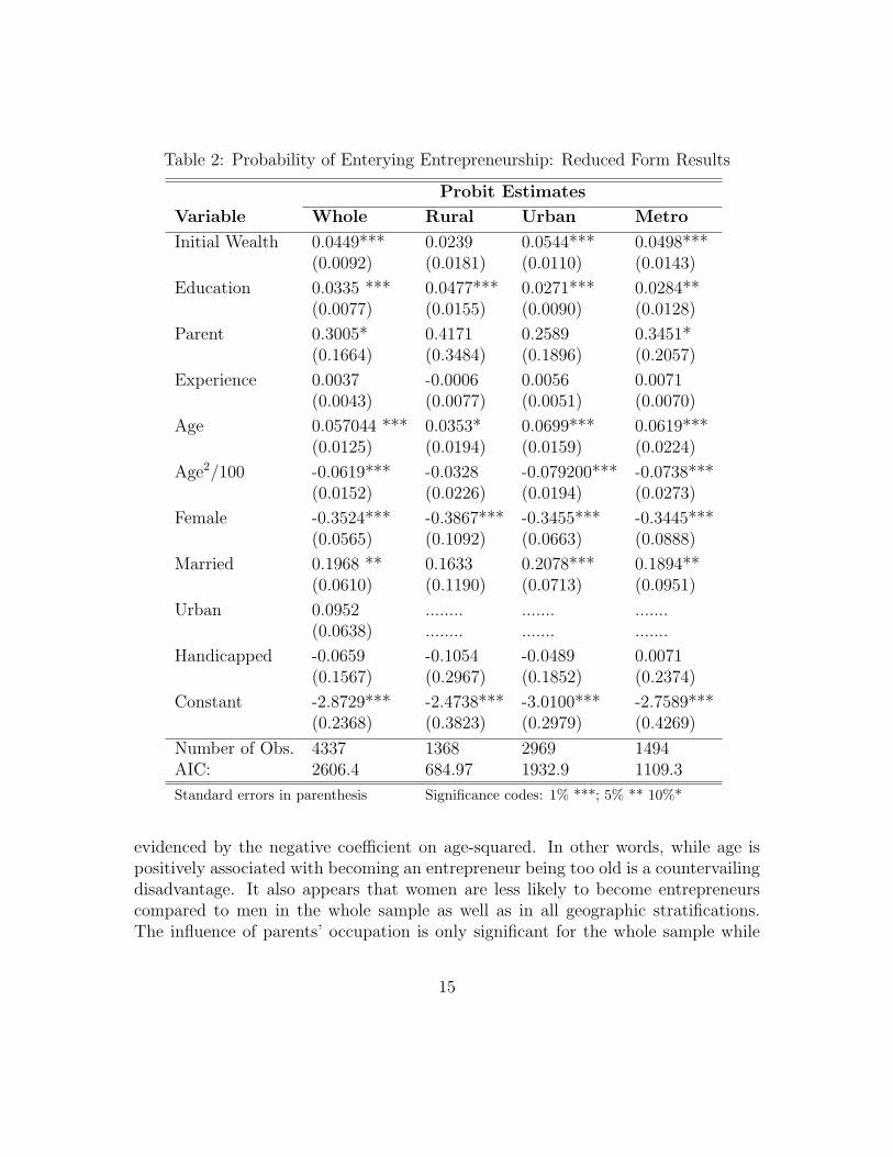
Table 2: Probability of Enterying Entrepreneurship: Reduced Form Results

Probit Estimates

Variable Whole Rural Urban Metro

Initial Wealth 0.0449*** 0.0239 0.0544*** 0.0498***(0.0092) (0.0181) (0.0110) (0.0143)

Education 0.0335 *** 0.0477*** 0.0271*** 0.0284**(0.0077) (0.0155) (0.0090) (0.0128)

Parent 0.3005* 0.4171 0.2589 0.3451*(0.1664) (0.3484) (0.1896) (0.2057)

Experience 0.0037 -0.0006 0.0056 0.0071(0.0043) (0.0077) (0.0051) (0.0070)

Age 0.057044 *** 0.0353* 0.0699*** 0.0619***(0.0125) (0.0194) (0.0159) (0.0224)

Age2/100 -0.0619*** -0.0328 -0.079200*** -0.0738***(0.0152) (0.0226) (0.0194) (0.0273)

Female -0.3524*** -0.3867*** -0.3455*** -0.3445***(0.0565) (0.1092) (0.0663) (0.0888)

Married 0.1968 ** 0.1633 0.2078*** 0.1894**(0.0610) (0.1190) (0.0713) (0.0951)

Urban 0.0952 ........ ....... .......(0.0638) ........ ....... .......

Handicapped -0.0659 -0.1054 -0.0489 0.0071(0.1567) (0.2967) (0.1852) (0.2374)

Constant -2.8729*** -2.4738*** -3.0100*** -2.7589***(0.2368) (0.3823) (0.2979) (0.4269)

Number of Obs. 4337 1368 2969 1494AIC: 2606.4 684.97 1932.9 1109.3

Standard errors in parenthesis Significance codes: 1% ***; 5% ** 10%*

evidenced by the negative coefficient on age-squared. In other words, while age ispositively associated with becoming an entrepreneur being too old is a countervailingdisadvantage. It also appears that women are less likely to become entrepreneurscompared to men in the whole sample as well as in all geographic stratifications.The influence of parents’ occupation is only significant for the whole sample while

15

the fact of being married does not affect the probability of starting a business in therural regions.

3.2.2 Quantile regressions

Another implication of the model is that since wealthier people start their businesseswith more efficient capital, the correlation between initial wealth and entrepreneurialearnings is positive. To investigate this issue, I run a quantile regression of log en-trepreneurial earnings on log initial wealth after controlling for education, experience,and several demographic characteristics. Given the high heterogeneity of informalenterprises earnings (see Figure 3), the quantile regression is an appropriate toolthat captures, better than the ordinary least squares regression, the specificities ofthe data as it permits to get estimates at different percentiles of the distribution.

Table 3 presents quantile regression estimates for the median, the first and thethird quarters of the distribution of earnings. The results show the positive andstatistically significant correlation of my measure of initial wealth and earnings atall quarters of the distribution of earnings. A similar result is obtained from OLSregression whose overall estimates are similar to those of the median regression.However, some important features that are not captured by the OLS regression butare by the quantile regression should be emphasized. While experience has no effecton the earnings of the remaining distribution of households, it positively influencesthe earnings of the poorer households (those of the top 25% percentile). This meansthat poorer households have to compensate their low investment by accumulatingmore experience in order to get a decent profit. Also, unlike the other groups, beinghandicapped negatively influences the earnings of richer households (those of the75% percentile). These results confirm that financially constrained firms will startwith a suboptimal amount of capital and will therefore earn smaller profit thanunconstrained firms.

4 Structural Estimation and Specification Analy-

sis

In this section I derive the likelihood function of the model and use it to producestructural parameter estimates. I also perform specification analysis and model di-agnostic tests using the Lavergne & Nguimkeu (2011) model specification test as wellas nonparametric regression checks. The goal is to use these structural estimates to

16

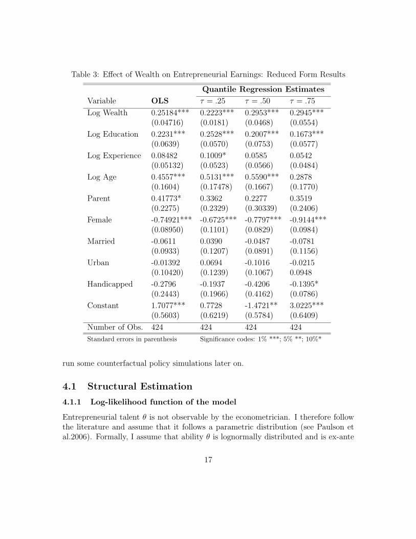
Table 3: Effect of Wealth on Entrepreneurial Earnings: Reduced Form Results

Quantile Regression Estimates

Variable OLS τ = .25 τ = .50 τ = .75

Log Wealth 0.25184*** 0.2223*** 0.2953*** 0.2945***(0.04716) (0.0181) (0.0468) (0.0554)

Log Education 0.2231*** 0.2528*** 0.2007*** 0.1673***(0.0639) (0.0570) (0.0753) (0.0577)

Log Experience 0.08482 0.1009* 0.0585 0.0542(0.05132) (0.0523) (0.0566) (0.0484)

Log Age 0.4557*** 0.5131*** 0.5590*** 0.2878(0.1604) (0.17478) (0.1667) (0.1770)

Parent 0.41773* 0.3362 0.2277 0.3519(0.2275) (0.2329) (0.30339) (0.2406)

Female -0.74921*** -0.6725*** -0.7797*** -0.9144***(0.08950) (0.1101) (0.0829) (0.0984)

Married -0.0611 0.0390 -0.0487 -0.0781(0.0933) (0.1207) (0.0891) (0.1156)

Urban -0.01392 0.0694 -0.1016 -0.0215(0.10420) (0.1239) (0.1067) 0.0948

Handicapped -0.2796 -0.1937 -0.4206 -0.1395*(0.2443) (0.1966) (0.4162) (0.0786)

Constant 1.7077*** 0.7728 -1.4721** 3.0225***(0.5603) (0.6219) (0.5784) (0.6409)

Number of Obs. 424 424 424 424

Standard errors in parenthesis Significance codes: 1% ***; 5% **; 10%*

run some counterfactual policy simulations later on.

4.1 Structural Estimation

4.1.1 Log-likelihood function of the model

Entrepreneurial talent θ is not observable by the econometrician. I therefore followthe literature and assume that it follows a parametric distribution (see Paulson etal.2006). Formally, I assume that ability θ is lognormally distributed and is ex-ante

17

correlated with initial wealth and formal education. I also extend the literature byallowing ability to be also correlated with informal entrepreneurial training which canbe captured by parents’ occupation.This assumption is motivated by a number ofempirical studies that found that the entrepreneurial ability of individuals increasesif their parents were also entrepreneurs, partly because children may receive informalbusiness skills from their parents (see, e.g. Lentz & Laband 1990, Parker & van Praag2006). One can therefore write

ln θ = δ0 + δ1 ln z + δ2 ln(1 + S) + δ3P + ε (11)

where z is the initial wealth, S are the years of education, and P is a dummy variabletaking 1 if at least one parent was an entrepreneur and 0 otherwise. The error termε is assumed to be normally distributed with mean 0 and variance σ2.

Recall from Section 2 that π(z, θ) is the comparative profit from choosing en-trepreneurship as opposed to subsistence activity. The allocation of households inentrepreneurship (E = 1) and subsistence (E = 0) can then be modeled as:

E = I{π(z, θ) ≥ 0} (12)

where I{·} is the indicator function that equals 1 if its argument is true and 0otherwise. We then have

Pr[E = 1] = Pr{π(z, θ) ≥ 0}= Pr{π(z, θ) ≥ 0|z ≥ z}Pr[z ≥ z] + Pr{π(z, θ) ≥ 0|z < z}Pr[z < z],

where the latter display follows from the law of total probability. Substituting z andπ(z, θ) by their expressions given in Formula (5) and Formula (7), respectively, weget

Pr{E = 1} = Pr{

(1− α)θ1

1−α(αr

) α1−α ≥ µ

}Pr

{z ≥ 1

λ

(θαr

) 11−α

}

+ Pr {θ(λz)α ≥ λrz + µ}Pr

{z <

1

λ

(θαr

) 11−α

} (13)

Taking the logs in the inequalities in the above terms yields

Pr{E = 1} = Pr

{ln θ > ln

( µ

1− α)1−α

(r

α

)α}Pr{

ln θ < lnr

α(zλ)1−α

}

+ Pr{

ln θ > ln(µ+ λrz)(λz)−α}

Pr{

ln θ > lnr

α(zλ)1−α

} (14)

18

If I now plug-in the distributional specification of ln θ given by Equation (11),I obtain the probability of becoming entrepreneur as a function of parameters andobservables

Pr{E = 1|X} = Φ(h1(ψ,X))Φ(−h3(ψ,X)) + Φ(h2(ψ,X))Φ(h3(ψ,X))

= H(ψ,X)(15)

where X = [1, z, S, P ]′ is the vector of covariates, ψ = [µ, δ0, δ1, δ2, δ3, α, σ, λ, r] is theset of parameters, and Φ(·) is the cumulative distribution function of the standardnormal. The functions hi(·), i = 1, 2, 3, appearing in Equation (15) are defined by

h1(ψ,X) =1

σ

{δ0 − (1− α) ln

µ

1− α− α ln

r

α+ δ1 ln(z) + δ2 ln(1 + S) + δ3P

},

h2(ψ,X) =1

σ{δ0 + α lnλ− ln(µ+ λrz) + (δ1 + α) ln(z) + δ2 ln(1 + S) + δ3P} ,

h3(ψ,X) =1

σ

{δ0 − (1− α) lnλ− ln

r

α+ (δ1 − 1 + α) ln(z) + δ2 ln(1 + S) + δ3P

}

(16)Given a sample of independent observations of size n, {(Ei, Xi), i = 1, . . . , n}, thelog-likelihood function of the econometric model can therefore be written as:

Ln(ψ) =n∑

i=1

{Ei lnH(ψ,Xi) + (1− Ei) ln(1−H(ψ,Xi))

}(17)

The gross interest rate r is exogenously fixed at 1.42, representing the observedaverage interest rate in the microfinance institutions in the country (see IDLO 2011).The maximum likelihood estimation is therefore performed over the set of parametersψ = [µ, δ0, δ1, δ2, δ3, α, σ, λ]. These parameters correspond respectively to the subsis-tence parameter µ, the constant term of the ability distribution, δ0; the interactionbetween wealth and ability, δ1; the interaction between education and ability, δ2; theinteraction between parents occupation and ability, δ3; the productivity of capital inthe production technology, α; the standard deviation of the ability distribution, σ;and the proportion of wealth, including outside funds, that can be invested, λ.

4.1.2 Structural Results

The maximum likelihood estimates of the model are reported in Table 4. The subsis-tence parameter µ is estimated at 37.2 for the whole sample and is higher in Urban

19

and Metro compared to rural areas. The constant term of log-ability expressed byδ0 is estimated at 3.36 for the whole sample and is also higher in the urban regioncompared to the rural region. The highest of the country is recorded at the Metroregion that includes the two main cities, Douala and Yaounde. This coefficient canbe regarded as the “natural” ability level, i.e. ability level that do not dependon the acquired observable characteristics. The estimated correlation between en-trepreneurial ability and household initial wealth δ1 is statistically insignificant forthe whole sample as well as for all the sample stratifications. This means that ourmeasure of household initial wealth is not acting as a proxy to entrepreneurial ability.The parameter estimates for δ2 indicates that there is a correlation between yearsof schooling and entrepreneurial ability. This parameter is estimated to be 0.091 forthe whole sample and means that each additional year of schooling can be associatedwith a 9.1% average increase in ability.

The parameter that relates parent occupation and entrepreneurial ability, δ3, isestimated to be 0.068 for the whole sample. Thus, having a parent who was anentrepreneur increases the entrepreneurial ability by 6.8%. In addition, this param-eter is positive and significant across stratifications and is higher in the Rural regionthan elsewhere. This result shows that parents occupation influence individuals en-trepreneurial ability. This finding is similar to that of Lentz & Laband (1990) whouse the National Federation and Independent Businesses (NFIB) data to show thathalf of self-employed proprietors are second-generation proprietors. The point esti-mate of 0.49 of the production parameter, α, means that a 1% increase in the capitaldevoted to a business leads to about 49% increase in income in the whole sample.The value of this parameter is even higher in the rural region. This suggests thatin the rural regions, households operate at a small scale with high marginal returns.Returns to capital therefore appear to be high in the informal sector compared tothose obtain for the formal sector. This result is consistent with those of many stud-ies performed in Africa (Kremer et al. 2010; Udry & Anagol 2006; Schundeln 2004). High returns to capital can then be regarded as indicative of the unexploited po-tential of informal entrepreneurs. The coefficient σ, is estimated at about 0.3 for thewhole sample and varies across geographical stratification. In particular, it is con-siderably lower in the rural areas as there is likely to be a less diverse variety of skills.

The degree of financial constraints is measured by λ and estimated at 12.6 for thewhole sample, 39.2 for the rural sample and 13.6 for the urban sample. This impliesthat households of the rural areas are less constrained than those of the urban areas.The most constrained entrepreneurs are those who operate in the Metro areas, wherethe parameter is estimated at 8.1. This result can be tied to the probit estimates

20

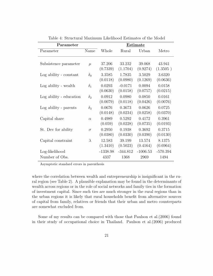
Table 4: Structural Maximum Likelihood Estimates of the Model

Parameter Estimate

Parameter Name Whole Rural Urban Metro

Subsistence parameter µ 37.206 33.232 39.068 43.941(0.7339) (1.1704) (0.9274) (1.3505 )

Log ability - constant δ0 3.3585 1.7835 3.5029 3.6320(0.0118) (0.0980) (0.1269) (0.0636)

Log ability - wealth δ1 0.0293 -0.0171 0.0094 0.0158(0.0630) (0.0158) (0.0757) (0.0215)

Log ability - education δ2 0.0912 0.0980 0.0850 0.0161(0.0079) (0.0118) (0.0426) (0.0076)

Log ability - parents δ3 0.0676 0.3673 0.0626 0.0725(0.0148) (0.0234) (0.0258) (0.0370)

Capital share α 0.4989 0.5292 0.4172 0.3961(0.059) (0.0228) (0.0735) (0.0193)

St. Dev for ability σ 0.2950 0.1938 0.3692 0.3715(0.0380) (0.0330) (0.0390) (0.0130)

Capital constraint λ 12.583 39.199 13.574 8.1375(1.3410) (0.5023) (0.4164) (0.6964)

Log-likelihood -1338.98 -344.812 -1006.53 -570.394

Number of Obs. 4337 1368 2969 1494

Asymptotic standard errors in parenthesis

where the correlation between wealth and entrepreneurship is insignificant in the ru-ral region (see Table 2). A plausible explanation may be found in the determinants ofwealth across regions or in the role of social networks and family ties in the formationof investment capital. Since such ties are much stronger in the rural regions than inthe urban regions it is likely that rural households benefit from alternative sourcesof capital from family, relatives or friends that their urban and metro counterpartsare somewhat excluded from.

Some of my results can be compared with those that Paulson et al.(2006) foundin their study of occupational choice in Thailand. Paulson et al.(2006) produced

21

estimates of α that ranged from 0.23 to 0.79. The estimate of α for the Camerooninformal sector is within this range at 0.49. The Cameroon talent estimates arenot directly comparable with the Thai estimates because the model I estimate al-lows talent to be correlated with parent’s occupation and Paulson et al. do not.Nevertheless, for Cameroon, the point estimate of δ0 is 3.35 whereas Paulson et al.estimate this parameter to be between 0.1 and 1.02. The correlation between talentand initial wealth, δ1, in both studies are similar and estimated at 0.29, althoughthe estimate for Cameroon is not statistically significant. A major difference be-tween the Cameroon findings and those of Thailand is on the estimates of δ2. TheCameroon data show a positive correlation between talent and schooling, estimatedat 0.09 whereas Paulson et al.(2006) found that schooling is negatively correlatedwith talent at −0.22. Likewise, the Cameroon credit constraint parameter λ is notdirectly comparable to the Thailand estimates because unlike Paulson et al. whoactually use data on total household asset my measure of initial wealth is an indexof household belongings. Nonetheless, they found that λ ranges from 10.7 to 21 andmy estimate of this parameter falls within this range at 12.6.

4.2 Specification analysis and robustness check

Since the estimated empirical model is just a simplification of the unknown truemodel, I perform a robustness check and a specification analysis to test the validityof the maximum likelihood estimates in order to get a sense of how reliable theyare for a counterfactual policy experiment. For the former, I perform nonparametricregression among the key variables of the model, and for the latter I use the Lavergne& Nguimkeu (2011) model specification test statistic.

4.2.1 Nonparametric evidence

Given that initial household wealth and education appear to be key factors influenc-ing entrepreneurial choice in the reduced form and structural results described above,I use nonparametric techniques to further test this evidence. I run a nonparametricregression of the probability of becoming an entrepreneur as a function of wealth,and as a function of wealth and education. Unlike the parametric methods, thenonparametric estimation does not impose any a priori functional form represen-tation of the relationship between variables that may alter the predictions, but onlypresumes that some regularity conditions such as differentiability are satisfied. I usekernel regression to estimate the probability of starting a business as a function of

22

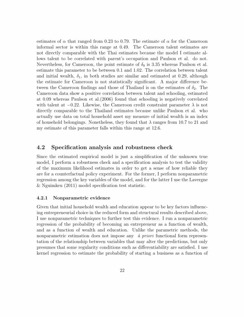
initial wealth and years of schooling respectively.14 Figure 4 pictures the estimatednonparametric relationships.

Figure 4: Nonparametric relation between Entrepreneurship and wealth (left) andEntrepreneurship, wealth and education (right)

0 5 10 15 20 25 300

0.05

0.1

0.15

0.2

0.25

0.3

Household Asset

Pro

ba

bil

ity

of

En

tre

pre

ne

urs

hip

Dashed line = +/!2 pointwise SE

Student Version of MATLAB

Asset

5

10

15

20

25

Education

0

5

10

15

Pro

bability

of E

ntre

pre

neurs

hip

0.05

0.10

0.15

0.20

0.25

As shown in the figure, there is a positive overall relationship between initialhousehold wealth and entrepreneurship. The point estimates show a strictly increas-ing and very precise pattern of the relationship at a lower level of initial householdwealth. For higher initial wealth levels however, the estimates display a somewhatflat relationship between wealth and the probability of entrepreneurship, which isconsistent with the theoretical model predictions as depicted in the stylized figuregiven by Figure 1. However, the standard errors bands at this latter pattern areextremely large so that the observed relationship between higher levels of wealthand entrepreneurship is in fact imprecise. This imprecision might come from thefact that the data contains only scanty observations at higher initial wealth levels asevidenced by Figure 3. The estimates also exhibit a strictly positive nonparametricrelation between years of schooling and the probability to start a business at all levelsof the education distribution. These nonparametric results are consistent with thosepreviously obtained from the reduced form and structural approaches.

14The methods are applied using cross-validated bandwidths. For references on this nonparamet-ric method, see Li & Racine (2007, pp. 60-100)

23

4.2.2 Model specification test

Recall that the econometric model I am estimating is given by

Pr{Ei = 1|Xi} = H(ψ,Xi) (18)

were H(ψ,Xi) is the probability of being an entrepreneur generated by the theoreticalmodel of Section 3 for a household i with observable characteristics Xi, given inEquation (15). Maximization of the sample log-likelihood function of this model

have produced a maximum likelihood estimate ψML which is consistent with thetrue parameter value ψ, and is asymptotically efficient, if the model is correctlyspecified. If the model is misspecified, this estimator is inconsistent for ψ and theestimation results are invalid because the estimated model is too far from the datagenerating process. To test the model, one can recast the problem in a conditionalmoment restriction (CMR) framework. To do this, observe that since the randomvariables Ei takes only two possible values 0 and 1, the model can be rewritten as

E[Ei −H(ψ,Xi)|Xi] = 0 (19)

For a sample of independent observations {(Ei, Xi), i = 1, . . . , n}, the conditions thatguarantee the identification and consistency of the MLE estimation of ψ are sufficientto estimate ψ from the CMR model (19) using smooth minimum distance (SMD)estimation method (see Lavergne & Patilea 2009).

Denote wi = (Ei, Xi) and m(wi, ψ) = Ei −H(ψ,Xi); The SMD estimator ψh solvesthe minimization problem

minψMn,h(ψ) =

1

2n(n− 1)

∑

1≤i 6=j≤n

m′(wi, ψ)W−1/2n (Xi)W

−1/2n (Xj)m(wj, ψ)Kij (20)

with Khij = h−qK

(Xi−Xjh

), where K(·) is the multivariate gaussian kernel, h is the

bandwidth parameter, and q corresponds to the dimension of X, excluding the con-stant. The weighting factor Wn(.) is defined by

Wn(x) =1

n

n∑

k=1

m(wk, ψML)m′(wk, ψML)b−qn K((x−Xk)/bn)).

with bn taken as n−1/5. Solving (20) with two different bandwidths b = 1 (a fixedbandwidth) and hn = cn−1/5 (a bandwidth that depends on the size n of the sample),

where c is an arbitrary positive constant, yields two SMD estimators ψb and ψhn

24

which are respectively consistent and semiparametrically efficient when the model iscorrectly specified, and both asymptotically normal.As proposed by Lavergne & Nguimkeu (2011), a Hausman-type specification teststatistics for Model (19) can be defined by

Tn = n(ψb − ψhn

)′Σ−1n

(ψb − ψhn

)(21)

The matrix Σn is a suitable standardized matrix whose expression is given in Ap-pendix 7.4. The test statistic Tn is asymptotically χ2

p (where p is the size of theparameter vector) distributed under the null of correct specification (see Lavergne &Nguimkeu 2011, Theorem 1), and takes significantly large values under the alterna-tive of misspecification.Using numerical optimization algorithms, I computed the values of the specificationtest statistic using the data, for different values of c, namely, c = 0.5; 1; 1.5. For thesevalues, Tn equals respectively to 15.102, 13.432, and 15.713, thus failing to reject themodel at a 5% significance level.

The results of the bandwidth Hausman test show that the model correctly fitsthe data at a 5% statistical significance. However, this result should be interpretedwith cautious. In fact, given the evident imprecision of the estimates of the effectsof initial wealth on entrepreneurship at high levels of initial wealth, as shown in thenonparametric estimation above (see Figure 4), it is hard to know whether the lack ofrejection is simply a power issue. Nonetheless, if one accepts that the model is correct,then it has significant implications on the nature of credit market imperfections andmisallocation of skills in the Cameroon informal sector. In particular, it shows thatobservable individual skills (such as education) do not matter to lenders in theirassessment of customers’ amount of loan or ability to repay, as does the collateral. Italso consolidates the non-obvious predictions of the model that among people withthe same initial wealth the higher skilled person is more likely to be constrainedbecause the optimal size of his business is larger. A natural and interesting questionthat arises is therefore to know what would be the impact on the economy if potentialentrepreneurs are allowed to borrow without the collateral requirements.

5 Counterfactual Policy Experiment

In this section, I use the structural estimates of the model to evaluate the impactof some policies on the informal sector. Since all my results suggested that accessto credit is one of the most important factors influencing occupations and earnings

25

in the informal sector, I consider the following strategy. I examine the effects of amicro-lending program on the fraction of entrepreneurs, the proportion of missingentrepreneurs, the heterogeneity among entrepreneurs captured by the ratio of con-strained versus unconstrained enterprises, and entrepreneurial earnings. But first, itis useful to know the initial state of the informal sector composition as produced bythe structural estimates, relative to which the simulated economy is compared.

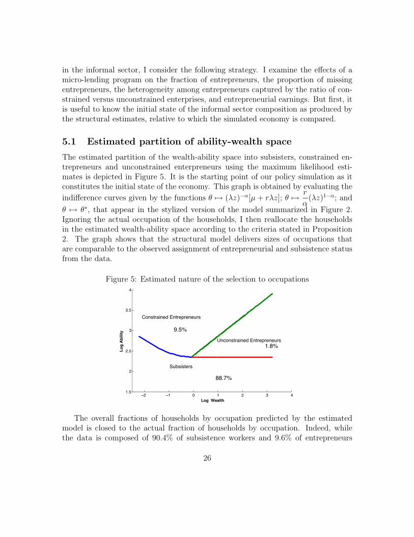
5.1 Estimated partition of ability-wealth space

The estimated partition of the wealth-ability space into subsisters, constrained en-trepreneurs and unconstrained enterpreneurs using the maximum likelihood esti-mates is depicted in Figure 5. It is the starting point of our policy simulation as itconstitutes the initial state of the economy. This graph is obtained by evaluating the

indifference curves given by the functions θ 7→ (λz)−α[µ + rλz]; θ 7→ r

α(λz)1−α; and

θ 7→ θ∗, that appear in the stylized version of the model summarized in Figure 2.Ignoring the actual occupation of the households, I then reallocate the householdsin the estimated wealth-ability space according to the criteria stated in Proposition2. The graph shows that the structural model delivers sizes of occupations thatare comparable to the observed assignment of entrepreneurial and subsistence statusfrom the data.

Figure 5: Estimated nature of the selection to occupations

!2 !1 0 1 2 3 41.5

2

2.5

3

3.5

4

Log Wealth

Lo

g A

bil

ity

Constrained Entrepreneurs

9.5%

88.7%

1.8%

Subsisters

Unconstrained Entrepreneurs

Student Version of MATLAB

The overall fractions of households by occupation predicted by the estimatedmodel is closed to the actual fraction of households by occupation. Indeed, whilethe data is composed of 90.4% of subsistence workers and 9.6% of entrepreneurs

26

the model predicts 88.7% of subsistence workers and 11.3% of entrepreneurs amongwhich about 9.5% are constrained and 1.8% are unconstrained (see percentages ap-pearing in Figure 5).

5.2 Microfinance Policy

Microfinance is a credit program targeting small-scale entrepreneurial activities ofthe poor who may otherwise lack access to credit because of absence of collateral.Following Buera et al.(2011), I quantify the effect of microfinance by relaxing indi-vidual capital rental limit as follows:

0 ≤ k ≤ max{λz, z + F} (22)

where F represents the additional capital provided by microfinance. Entrepreneurstherefore choose to borrow from the traditional financial institutions subject to thecollateralized borrowing limit λz as discussed in our previews sections, or to useMicrofinance to get additional funding on top of their initial capital, z + F . Thistopped-up funding is a lump-sum amount that is independent of their initial wealthor entrepreneurial ability. Practically, the microfinance policy may be initiated by agovernment-sponsored agency that guarantees small loans for business start-ups, suchas the US Small Business Administration (SBA) or the British Enterprise AllowanceProgram (BEAP). Other examples from developing countries include the NABARDin India (a government rural development bank that supports small-scale saving andinternal lending from self help groups), the BRI in Indonesia (Bank Rakayat Indone-sia, that promotes microloans to small and medium-scale enterprises), or the PCFCin Philippines (People’s Credit and Finance Corporation, that is mandated by lawto supplement loans to the poor through wholesale funds to retail microfinance in-stitutions) (See Kaboski & Townsend 2010, Buera et al.2011, for a review).

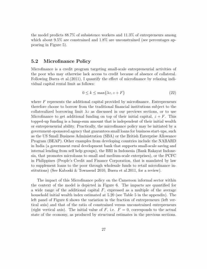
The impact of this Microfinance policy on the Cameroon informal sector withinthe context of the model is depicted in Figure 6. The impacts are quantified fora wide range of the additional capital F , expressed as a multiple of the averagehousehold initial wealth index estimated at 5.20 (see Table 5 in the appendix). Theleft panel of Figure 6 shows the variation in the fraction of entrepreneurs (left ver-tical axis) and that of the ratio of constrained versus unconstrained entrepreneurs(right vertical axis). The initial value of F , i.e. F = 0, corresponds to the actualstate of the economy, as produced by structural estimates in the previous sections.

27

Figure 6: Impacts of Microfinance policy

0 1 2 3 4 5 610

12

14

16

18

20

F/z

Pro

por

tion

(%)

0 1 2 3 4 5 63.5

4

4.5

5

5.5

6

fr ac. Entrepreneurs

rat io Cons tr./Unconst.

Student Version of MATLAB

0 1 2 3 4 5 662

64

66

68

70

72

74

76

78

80

F/z

Ear

nin

gs

Entrep. earnings

Total earnings

Student Version of MATLAB

We observe two clear patterns. First, the fraction of entrepreneurs substantially in-creases with increasing values of F , from about 11% to reach a steady proportionclose to 20%, representing almost twice the initial fraction. The maximum size ofentrepreneurs is reached when the available funding is up to 3.5 times the value ofthe average household initial wealth, z. This shows that, because of financial con-straints, the country is “missing” about 9% of informal entrepreneurs, that is, aboutthe same fraction currently available in the raw data. Second, the ratio of constrainedover unconstrained entrepreneurs slightly increases with smaller increases in F , thensteadily decreases with higher values of F . This is because for smaller values of F ,many talented households will move from subsistence to entrepreneurship, but willremain constrained since the capital at their disposal may not be enough to opti-mally implement their project. Thus the ratio of constrained over unconstrained willincrease. However, for larger amounts of F , many talented households will movefrom subsistence to directly run unconstrained firms while constrained entrepreneurswill become unconstrained as well. The ratio of constrained over unconstrained willthen drastically decrease.

The right panel of Figure 6 shows that entrepreneurial earnings and total in-formal sector earnings increase with F . We observe an increase of about 15% ofentrepreneurial earnings when F grows from 0 to 5z, and an increase of about 30%of total earnings for the same increase in F .15 While both quantities increase, itis worth noticing that the gap between total earnings and entrepreneurial earningsconsistently decreases with increasing values of F . This means that the earningsdifferentials in the informal sector get smaller as people get more access to credit.

15All quantities represented in this simulation figure are averages.

28

These findings are consistent with several other studies that have shown how mis-allocations of capital that arise from credit constraints, limited loan enforcementor institutions and policy distortions can cause important total factor productiv-ity (TFP) gaps across firms or between countries and how appropriate policy couldremedy the situation ( see Restuccia and Rogerson 2008; Hsieh and Klenow 2009;Banerjee and Moll 2010; ).

The results obtain in this experiment are based on the assumption that peoplewho borrow from microfinance fully repay their loans at the end of the period. Be-cause I am estimating a partial equilibrium model, I am thus completely abstractingfrom the expected costs incurred by people who may default the repayment of theirloan as well as the costs involved with running microfinance. These results shouldtherefore be regarded as the upper bound of the benefits of microfinance. However,given the extremely low or insignificant rates of default encountered in Microfinanceas found in various empirical studies (see Field and Pande 2008; McIntosh 2008) itis expected that the results presented here would not be significantly affected even ifthe cost of defaults in this microfinance policy was incorporated via a more generalframework. The simulations therefore suggest that microfinance could be a suitabletool not only to reduce poverty and increase entrepreneurship (by increasing jobcreation and earnings in the informal sector) but also to lower the heterogeneity ofoccupations and earnings observed in the informal sector (by reducing misallocationof capital and skills).

6 Concluding Remarks

This paper provides an econometric analysis of the heterogeneity observed in the in-formal sector, whose main characteristics are its diversity and segmentation featuringmassive proportion of subsisters who coexist with a handful of microentrepreneurs.I use a simple theoretical model of occupational choice where agents differ withtheir initial wealth and skills, to analyze the implications of financial constraints onearnings, occupational patterns and entrepreneurship in the informal sector. Theimplications of the model are tested using reduced form estimates including pro-bit and quantile regressions over multivariate controls, as well as nonparametricregressions. The results suggest that initial wealth and education are the main fac-tors that strongly influence both the probability of becoming entrepreneur and theentrepreneurial earning. These results show evidence of the existence of financialconstraints in the economy.

29

The theoretical model is also structurally estimated using maximum likelihood.The results suggest that there are high returns to capital of about 50% in the informalsector. The capital constraints, however, appear to be weaker in rural regions than inurban and metro areas. The adequacy of the empirical model with the data is checkedthrough a model specification test which confirms that the model is consistent withthe data at a 5% statistical significance level. The potential of the theoretical modelto generate differences in earnings and occupational patterns that match the datafrom Cameroon is then exploited to evaluate and quantify the impact of economicpolicies on the informal economy using its estimated version. Counterfactual experi-ments show that a micro-lending program aiming at providing more access to creditto the poor, substantially increases the fraction of microentrepreneurs and reducesthe proportion of poor in the economy. Roughly, microfinance can reduce the sizeof subsistence by up to 10% while almost doubling the fraction of entrepreneurs inthe informal sector. Moreover, when abstracting from possible defaults costs, micro-finance can improve the total earnings capacity of the informal sector by up to 30%,and has the potential of lowering heterogeneity, by reducing misallocations of skillsand capital.

To the best of my knowledge, the structural test of the role of financial constraintsand availability of skills in explaining heterogeneity and occupational patterns andproviding a ground for policy interventions in the informal economy performed inthis study is new to the literature. There are however many directions in whichthis research can be improved and extended. In fact, because the formal sectoris absent in this study, the model does not allow to derive a general equilibriumthrough which the phenomenon of informal sector can be quantified over the rest ofthe economy. For example, although it is intuitively clear that the increase of small-scale enterprises due to microfinance, as implied by our model, would have extensivebeneficial consequences on the demand for capital goods for production use in theformal industrialized sector, our framework does not allow to quantify such benefits.These considerations are left for further studies.

30

7 Appendix

7.1 Additional tables and figures

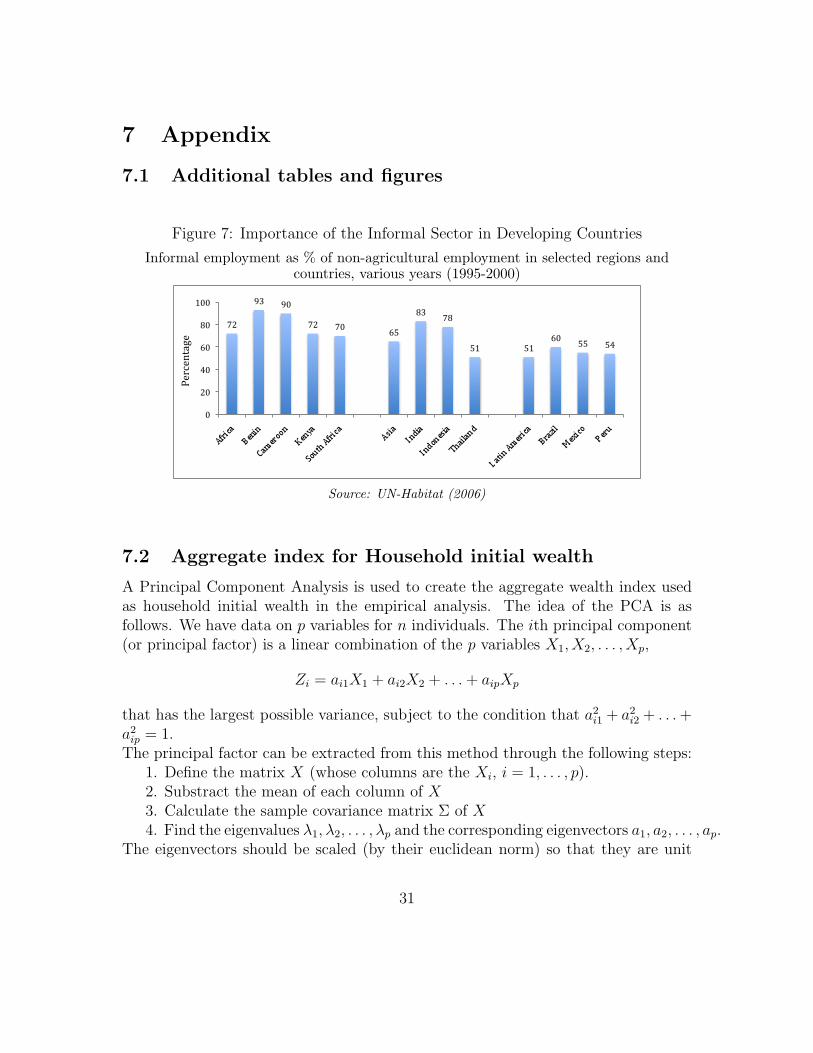
Figure 7: Importance of the Informal Sector in Developing Countries

Informal employment as % of non-agricultural employment in selected regions andcountries, various years (1995-2000)

!

!

!

!

Region Number of

Procedures

Duration

(Days)

Cost as

Percentage of

GNI/capita

OECD 6 25 8

South Asia 9 46 45.4

East Asia and the Pacific 8 51 47.1

Middle East and North Africa 10 39 51.2

Latin America and the Caribbean 11 70 60.4

Subsahara Africa 11 63 225.2

!

"#!

$%! $&!

"#! "&!'(!

)%!")!

(*! (*!'&!

((! (+!

&!

#&!

+&!

'&!

)&!

*&&!

,-./-0123-!

Source: UN-Habitat (2006)

7.2 Aggregate index for Household initial wealth

A Principal Component Analysis is used to create the aggregate wealth index usedas household initial wealth in the empirical analysis. The idea of the PCA is asfollows. We have data on p variables for n individuals. The ith principal component(or principal factor) is a linear combination of the p variables X1, X2, . . . , Xp,

Zi = ai1X1 + ai2X2 + . . .+ aipXp

that has the largest possible variance, subject to the condition that a2i1 + a2

i2 + . . .+a2ip = 1.

The principal factor can be extracted from this method through the following steps:1. Define the matrix X (whose columns are the Xi, i = 1, . . . , p).2. Substract the mean of each column of X3. Calculate the sample covariance matrix Σ of X4. Find the eigenvalues λ1, λ2, . . . , λp and the corresponding eigenvectors a1, a2, . . . , ap.

The eigenvectors should be scaled (by their euclidean norm) so that they are unit

31

Table 5: Household Characteristics in the Cameroon informal sector

Estimate

Characteristics Whole Rural Urban Metro

Number of obs. 4337 1368 2969 1494% of sample 100% 40.2% 59.8% 31.1%

% of women 54.3% 57.0% 52.8% 52.6%

Av. household size 6.0 6.2 6.1 5.3

Av. age of head 35.4 35.9 35.1 35.5Years of schooling

0-5 years 43.7% 56.8% 36.5% 23.6%6-10 years 45.2% 37.0% 49.6% 57.3%

11+years 11.1% 6.2% 13.9% 19.1%

Av. income* 58.61 41.87 62.28 69.66Av. wealth index 5.205 2.146 5.693 6.476

*In thousands of local currency (CFA); 1, 000CFA ∼ $2US Source: Own calculations

vectors. The coefficients of the ith principal component are then given by ai whileλi is its variance.

5. Assuming that the eigenvalues are ordered as λ1 ≥ λ2 ≥ . . . ≥ λp, choose theeigenvector that is associated with the highest eigenvalue, that is a1. The principalcomponent then corresponds to the eigenvector a1,

Z1 = a11X1 + a12X2 + . . .+ a1pXp

In particular, Var[Z1] = λ1 which is the highest possible variance.To construct this single index, I use some household items in the questionnaire thatrelate to the number of durable goods in the household: number of vehicles, numberof TVs, number of radios, number of DVD/Video-CD, number of fridges, numberof freezers, number of gas cookers, number of fans, number of sewing machines, adummy variable that is equal to 1 if the household has air conditioning, number ofmobile phones, number of computers, number of electric irons, number of housesowned by the household. We consider only items that were acquired by the house-holds prior their entry to their current activity. The resulting index computed fromthe data explains 31% of the variance in households durables.

32

Table 6: The cost of regulation: Requirement to start a formal business

Region Number of Duration Cost as PercentageProcedures (Days) of GNI/capita

OECD 6 25 8South Asia 9 46 45.4East Asia and the Pacific 8 51 47.1Middle East and North Africa 10 39 51.2Latin America and the Caribbean 11 70 60.4Subsahara Africa 11 63 225.2

Source: UN-Habitat (2006)

7.3 Proof of Proposition 1

(i) The function π(·, θ) is continuous on R+ and differentiable on R∗+ and we have:

∂π(z, θ)

∂z=

0 if z ≥ z

αθλαzα−1 − λr if 0 < z < z(23)

Recall that z =1

λ

(θα

r

)1/(1−α)

. We can then rewrite (23) as :

∂π(z, θ)

∂z=

0 for z ≥ z

λr

([z

z

]1−α

− 1

)for 0 < z < z

(24)

It then follows that∂π(z, θ

∂z≥ 0, for all z.

(ii) From part (i) above, we know that the function π(·, θ) is increasing and has itsmaximum value at z. We can write

π(z, θ) = θ(λz)α − λrz − µ

= (1− α)θ1/(1−α)

(α

r

)α/(1−α)

− µ

= (1− α)

(α

r

) α1−α [

θ1

1−α − θ∗1

1−α]

(25)

33

For θ ≤ θ∗, we have π(z, θ) ≤ 0, and hence π(z, θ) ≤ 0 for all z.(iii) Suppose θ > θ∗, then from Expression (25) above, we see that π(z, θ) > 0. Onthe other hand, we have π(0, θ) = −µ < 0. By the Intermediate Value Theorem,there exists z ∈ (0, z) such that π(z, θ) = 0. By the monotonicity of π(·, θ) obtainedin part (i), it follows that π(z, θ) < 0 ∀z < z and π(z, θ) > 0 ∀z > z.�

7.4 Standardizing matrix in the Lavergne-Nguimkeu teststatistic

The expression of Σn used in the test statistic given in Equation ?? can be obtained as

Σn = V −1b ∆bV

−1b − V −1

0 where the respective matrices estimators Vb, ∆b, and V0

are given by

1

n(n− 1)

∑

i 6=j

∇θm(wi, ψb)W−1/2n (Xi)W

−1/2n (Xj)∇′θm(wj, ψn)b−qK

(Xi −Xj

b

),

1

n

∑

i

∇θm(wi, ψn)W−1n (Xi)fn(Xi)∇′θm(wi, ψn) and

1n(n−1)(n−2)

∑i 6=k,j 6=k∇θm(wi, ψb)W

−1/2n (Xi)W

−1/2n (Xk)∇′θm(wk, ψb)f

−1n (Xj)

b−2qK(Xi−Xj

b

)K(Xj−Xk

b

),

where fn(Xi) = 1n−1

∑j 6=i h

−qK((Xi −Xj)/h)) is the leave-one-out kernel estimatorof f(Xi)

7.5 Endogenizing financial constraints

I show here how the proportionality factor λ that is exogenously imposed in thetheoretical model to capture the existence of financial constraints due to imperfectenforceability of capital rental can arise endogenously. Suppose that borrowers mayvoluntarily default. In that case they keep their entrepreneurial income θkαε butloose their collateral z. However, with probability φ they can be caught, in whichcase the fraction of wealth βz is forfeited. Thus, borrowers who choose to defaultreceive a payoff of θkαε−φβz while those who choose to repay receive θkαε+r(z−k).Since the lenders are only willing to lend to those who will choose to repay, theincentive compatibility constraint is θkαε + r(z − k) ≥ θkαε − φβz. This impliesthat lenders will only rent to households whose wealth is sufficiently high, that is,

34

z ≥ r

r + βφk. Equivalently, this means that the capital that will be invested by the

household satisfies k ≤(

1 +βφ

r

)z.

35

References

[1] Aghion, Phillippe and Patrick Bolton 1996. A Trickle-down Theory of Growthand Development with Debt Overhang. Review of Economic Studies 64 (2),151172.

[2] Alby, P., Auriol, E., and Nguimkeu, P. 2011. Social Barriers to Entrepreneurshipin Africa: The Forced Mutual Help Hypothesis. Unpublished Manuscript.

[3] Banerjee, Abhijit and Andrew Newman 1993. Occupational Choice and theProcess of Development. Journal of Political Economy 101, 274 - 298.

[4] Banerjee, A., and E. Duflo 2004. Do Firms Want to Borrow More? Test-ing Credit Constraints Using a Directed Lending Program. UnpublishedManuscript.

[5] Banerjee, A., and B. Moll. 2010. Why Does Misallocation Persist? AmericanEconomic Journal: Macroeconomics, 2(1): 189-206.

[6] Buera, F., Kaboski, J. and Shin Y. 2011. The Macroeconomics of Microfinance.Unpublished Manuscript

[7] Cunningham, W. and Maloney,W.F. 2001. Heterogeneity among Mexicos Mi-croenterprises: An Application of Factor and Cluster Analysis. Economic De-velopment and Cultural Change 5, 131-156.

[8] De Mel, S., McKenzie, D., and Woodruff, C. 2008. Returns to Capital in Mi-croenterprises: Evidence from a Field Experiment. The Quarterly Journal ofEconomics, 123(4), 1329-1372.

[9] Duflo, E., Kremer, M. and Robinson, J. 2009. Nudging Farmers to use Fertilizer:Evidence from Kenya. Mimeo, MIT, Boston.

[10] Evans, David S. and Boyan Jovanovic. 1989. An Estimated Model of En-trepreneurial Choice under Liquidity Constraints. Journal of Political Economy97, 808- 827.

[11] ECAM II 2001. Deuxieme Enquete Camerounaise aupres des menages - Resumeexecutif. Institut National de la Statistique.

[12] Fields, G. S. 1990. Labor Market Modeling and the Urban Informal Sector:Theory and Evidence: in The Informal Sector Revisited. ed. David Tumham,Bernard Salome, and Antoine Schwartz (Paris: OECD, 1990)

36

[13] Field, E., and R. Pande 2008. Repayment Frequency and Default in Microfi-nance: Evidence From India. Journal of the European Economic Association,6(2-3), 501-509.

[14] Ghatak, M. and Jiang, N. 2002. A Simple Model of Inequality, OccupationalChoice, and Development. Journal of Development Economics, 69(1), 205-226.

[15] Gine, X. and R. Townsend 2004. Evaluation of Financial Liberalization: AGeneral Equilibrium Model with Constrained Occupational Choice. Journal ofDevelopment Economics, 74, pp. 269-307.

[16] Grimm, M., Kruger, J. and Lay, J. 2010. Barriers of entry and capital returns ininformal activities: Evidence from Sub-Saharan Africa. The Review of Incomeand Wealth, 57, 27-53.

[17] Grimm, M., F Gubert, O. Koriko, J. Lay, C. J. Nordman 2011. Kinship-ties andentrepreneurship in Western Africa. mimeo DIAL.

[18] Hsieh, Chang-Tai, and Peter Klenow. 2009. Misallocation and ManufacturingTFP in China and India. Quarterly Journal of Economics, 124 (4), 1403-1448

[19] International Development Law Organization 2011. Consumer Protection andMicrofinance: Country Reports. Legal Empowerment Working Paper series.

[20] International Labour Organisation 2002. Decent Work and the Informal Econ-omy. International Labor Conference.

[21] International Labour Organisation 2009. Trade Unions and the Informal Sector.International Labor Conference.

[22] Kremer,M., Lee,J.N. and Robinson, J.M. 2010. The return to capital for smallretailers in Kenya: Evidence from Inventories. Mimeo, Havard University

[23] Kuchta-Helbling C. 2000. Barriers to Participation: The Informal Sector inEmerging Democracies”, Center for International Private Enterprise

[24] Lavergne, P. and Nguimkeu, P. 2011. A Hausman Specification Test of Condi-tional Moment Restrictions. Unpublished Manuscript.

[25] Lavergne, P. and Patilea, V. 2009. Smooth Minimum Distance Estimationand Testing in Conditional Moment Restriction Models: Uniform-in-BandwidthTheory. Unpublished Manuscript.

37

[26] Li, Q. and Racine, J.S., 2007. Nonparametric Econometrics: Theory and Prac-tice. Princeton University Press.

[27] Lentz, B. F., and Laband, D.N., 1990. Entrepreneurial Success and OccupationalInheritance among Proprietors. The Canadian Journal of Economics, 23(3) 563-579

[28] Lloyd-Ellis, Huw and Dan Bernhardt 2000. Enterprise, Inequality and EconomicDevelopment. Review of Economic Studies 67, 147 - 168.

[29] Lucas Jr., R.E., 1978. On the size distribution of business firms. Bell Journal ofEconomics 9, 508523.

[30] McIntosh, C. 2008. Estimating Treatment Effects from Spatial Policy Exper-iments: An Application to Ugandan Microfinance. Review of Economics andStatistics, 90(1), 15-28.

[31] Mondragon-Velez, C. and Pena, X. 2009. Business Ownership and Self-Employment in Developing Economies: The Colombian Case. Manuscript.

[32] Nillesen, E.E.M., Beekman, G., and Gatto, M., 2011. Kinship Networks andInvestment in post-war Liberia. Unpublished Manuscript.

[33] Nguetse, P.J. 2009. Estimating the returns to education in Cameroon informalsector. The International Statistical Institute.

[34] Parker S. and Van Praag, M. 2010. The Entrepreneur’s Mode of Entry: BusinessTakeover or New Venture Start. Journal of Business Venturing

[35] Paulson, A., R. Townsend and A. Karaivanov, 2006. Distinguishing LimitedCommitment from Moral Hazard in a Model of Entrepreneurship. Journal ofPolitical Economy, 144(1), pp. 100-44.

[36] Piketty, T., 1997. The Dynamics of the Wealth Distribution and the InterestRate with Credit Rationing. Review of Economic Studies, 64(2), pp. 173-89.

[37] Restuccia, Diego, and Richard Rogerson 2008. Policy Distortions and AggregateProductivity with Heterogeneous Plants. Review of Economic Dynamics, 11,707720.

[38] Udry, C. and Anagol S. 2006. The return to capital in Ghana. American Eco-nomic Review 96 (2) 388-393.

38

[39] UN-Habitat 2006. A look at the Urban Informal Economy. United Nations Hu-man Settlement Programme, Vol. 13, No. 2.

[40] Schundeln, M., 2004. Modeling Firm Dynamics to Identify the Cost of FinancingConstraints in Ghanaian Manufacturing. Mimeo, Harvard University.

39