Z

d,

..... ~ : R. & M. No. 3687

• f ,

MINISTRY OF DEFENCE (PROCUREMENT EXECUTIVE)

AERONAUTICAL RESEARCH COUNCIL

REPORTS A N D MEMORANDA

A Streamline Curvature Through-Flow Computer Program for Analysing the Flow through

Axial-Flow Turbomachines By D. H. FROST

National Gas Turbine Establishment

L O N D O N : HER MAJESTY'S STATIONERY OFFICE 1972

PRICE 1"30 NET

A Streamline Curvature Through-Flow Computer Program for Analysing the Flow through

Axial-Flow " /~ Turbomachlnes:, ~ , . , ~%

By D. H_. FROST ,,L ,- ';%" ,,/ ,"

National Gas Turbine Establishment ~ .... b

Reports and Memoranda No. 3 6 8 7 * August, 1970

o , .V)~

Summary. This Report describes a computer program for the analysis of the fluid motion in the meridional

plane of axial flow turbomachines. The method uses a streamline curvature approach and the program allows calculations within blade rows. Comparisons with experiment and various other methods of analysis are presented.

LIST OF CONTENTS

1. Introduction

2. Method of Solution

2.1. The calculating grid

2.2. The calculations for one overall iteration

2.2.1. The calculation on a general plane

2.2.2. Stream function

2.3. Evaluation of terms in principal equations

2.3.1. Calculation of absolute swirl velocity

2.3.2. Calculation of stagnation enthalpy

2.3.3. Calculation of entropy

3. Numerical Examples

3.1. Two-stage turbine

3.1.1. Overall performance

*Replaces NGTE Report No. R.312--A.R.C. 32 776.

LIST OF C O N T E N T S - - c o n t i n u e d

3.2.

3.1.2. Flow profiles

3.1.3. Annulus wall static pressure distributions

3.1.4. Effects of blade blockage and radial tilt

Single-stage compressor

3.2.1. Results

4. Conclusions

Notation

References

Appendices No. I

II

III

Fig. No.

1

2

3

4

5

6

7

10

11

12

Derivation of principal equations

Adjustment of axial velocity

Conservation of rothalpy

LIST OF ILLUSTRATIONS

Title

An element of the meridional stream sheet

Mean stream surface angles 2' and #'

A typical grid

Forms of curve obtained from the velocity iteration

Form of curve obtained from the mass flow iteration

Streamline intercepts

Turbine--50 per cent design speed. Axial velocity profiles through second stage.

Turbine--87.5 per cent design speed. Axial velocity profiles through second stage.

Turbine--50 per cent design speed Far downstream flow profiles

Turbine--87.5 per cent design speed Far downstream flow profiles

Turbine--50 per cent design speed Comparison of static pressures

Turbine--87.5 per cent design speed Comparison of static pressures

LIST OF ILLUSTRATIONS--continued

13

14

Turbine--87.5 per cent design speed Far downstream : effects of blade blockage and blade tilt

Turbine--87-5 per cent design speed Interstage : effects of blade blockage and blade tilt

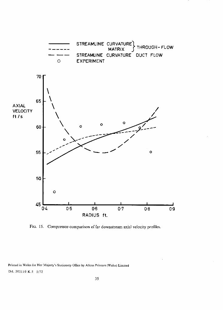
15 Compressor---comparison of far downstream axial velocity profiles

1. Introduction. The complete analysis of the flow through a turbomachine is a complex, three-dimensional problem

which, for practical purposes, must, at present, be regarded as insoluble, even with the present day size of computers and the advanced techniques available. The problem is therefore reduced to two separate and more manageable problems known as the hub-to-tip and the blade-to-blade.

The aim in the hub-to-tip problem is to solve for the flow only on a meridional surface of the turbo- machine. This approach has its origins in the Mean Line method, developed by Howell 1'2 for compressors and Ainley and Mathieson 3 for turbines, in that the meridional surface is collapsed onto a mean line through the machine. The flow is only calculated in the duct regions between adjacent blade rows on this mean line. The Streamline Curvature Duct Flow method, developed in the United States of America by Novak 4 and Smith 5 and, in the United Kingdom by Silvester and Hetherington 6 of Rolls Royce and the National Gas Turbine Establishment (NGTE), went a stage further by calculating the flow on a meridional plane right across the annulus but the solution is still restricted to the duct regions. However, Marsh 7, in his Matrix Through-Flow method, was able to extend the calculations to go within the blade rows by means of the specification of a meridional stream surface. This method employs a finite-difference technique rather than a streamline curvature approach for solving the equations and is restricted to subsonic relative flow within the blade rows. In the same way, it is possible to adapt the streamline curvature approach so as to be able to calculate the flow within blade rows, by introducing the concept ofa meridional stream surface. This Report describes a computer program for such a method which will be referred to as the Streamline Curvature Through-Flow method.

Since the two through-flow methods solve the same equations and make the same assumptions, the results obtained from them should be the same. However, the Streamline Curvature Through-Flow method is, in theory, capable of obtaining supersonic solutions with the restriction that the meridional Mach number should not exceed unity anywhere in the turbomachine. Also, the Streamline Curvature method requires far less computer storage than does the Matrix method.

Section 2 presents in detail the techniques employed in solving the principal equations which are derived from the basic aerodynamic and thermodynamic relationships in Appendix 1. This work is not essential to the understanding of the results given in Section 3. Results have been obtained for a two- stage, highly loaded axial flow turbine and a single-stage low pressure ratio compressor. These are compared with experimental data and with predictions from the Streamline Curvature Duct Flow and the Matrix Through-Flow methods. Furthermore, the discrepancies in the results from the two Stream- line Curvature programs have been investigated with a view to assessing the advantages and disadvantages of taking account of the flow within the blade passages.

The method described in this Report has been programmed in basic IBM Fortran IV for an SDS 90/300 computer with a core store of 32K and can therefore be run on a variety of computers with only minor alterations.

2. Method of Solution.

The principal equations to be solved are derived from the basic flow equations for inviscid, steady

3 flow in Appendix I, making use of Figures 1 and 2. Special derivatives of the form - - , - - , representing

r g the rate of change along the meridional stream surface, are defined and a blade blockage parameter B is introduced. Here, it suffices to state the principal equations obtained.

l ~p _ Wz 2 Itan22+½

p Or (1 - M z 2 sec2~) ~(tan22)0r I-(1-Mz2) tarZe dz2J _

Wz 2 t a n 2 1 dB

(1 - -Mz 2 sec22) (1 - B ) dz

4- [(1 - - Mz 2) tan 2' + Mz 2 tan ~. tan #'] Wz d(rVo) r dz

0)

~h Os 1 ~p and ~ = T ~rr+p 3 r ' (2)

The solution of these equations is obtained by an iterative technique at a discrete number of points. In the section that follows, a detailed description is presented of the method of solution and the numerical techniques employed.

2.1. The Calculatin9 Grid.

The flow field over which the equations are solved is bounded on two sides by the inner and outer annulus walls of the turbomachine (except for possible boundary layer allowance) and on the other two sides by the upstream and downstream boundaries, Figure 3. These boundaries must be normal to the axial direction. The grid is formed by calculating planes parallel to the upstream and downstream boundaries, each plane having an odd number of equally spaced grid points, the same number for each plane, between the inner and outer annulus walls. The spacing of the calculating planes need not be uniform and where necessary can be varied locally to provide a detailed picture of the flow.

Boundary conditions.

For the upstream boundary, the flow conditions on the first two planes, i = 1 and i = 2, of the flow field are specified to be uniform across the annulus and equal to the inlet flow conditions. These are calculated from the known mass flow and inlet stagnation temperature and pressure.

For the downstream boundary, the flow conditions on the last two planes, i = N - 1, i = N, of the grid are taken to be equal to the flow conditions calculated at the plane i = N - 2 .

The boundary condition applied at the annulus walls is that no flow crosses these boundaries, that is, the annulus walls are streamlines.

2.2. The Calculations for One Overall Iteration.

The equations used in this calculation are equation (1) and equation (2) put in simple finite difference form, thus

ri,j+ 1 - - ri,j 2 \rid+ 1 -- ri,j/t \ 2 /

, 1 @ wnere P c~r has been denoted as a and the subscripts refer to adjacent grid points on the calculating plane.

Re-arranging, we get

hi j+ ~ - h i j 1 . , ~ (Ti j+ ~ + Ti,j) (Si,j + 1 1 = - s ~ , j ) +-~ (cry,j+ ~ + ~r~,i) (r~a + ~ - r~j) (3)

2.2.1. The calculation on a general plane. The calculation takes the form of an integration of equation (3) commencing at the mid-radius grid point and proceeding step by step first to the outer wall and then to the inner wall. The guess for the mid-radius axial velocity needed to start off the integration is taken to be equal to its value on the previous overall iteration except on the first iteration, when the mid-radius axial velocity from the previous calculating plane is used.

Consider the integration from the mid-point to the outer casing. Knowing the flow conditions at a grid point (i,j), the corresponding axial velocity at (i,j + 1), denoted by Wz ( i , j+ 1), can be found by iteration, as follows. A guess, represented as W X , is made for W~ ( i , j+ 1). Given Wz at any grid point, it is possible to determine the flow completely at that point, from a knowledge of the mass flow distribu- tion, taken from the previous overall iteration, and the flow conditions on the previous plane. For the first iteration, it is assumed that the flow per unit area is constant across the annulus for all calculating planes. Thus, T~,j+ ~ and s~,j+ 1 can be evaluated and ~,i+ 1 can be obtained from equation (1). The methods used for calculating these quantities are described in Section 2.3. Using equation (3), the static enthalpy h~j+ 1 is determined and hence, from the energy equation, a new value of W~(i, j+ 1) = W Y obtained. Starting with a new W X , a new W Y is calculated and this process is continued until W X is within 0.01 ft/s of W Y . Details of the adjustment of W X are given in Appendix II and on Figure 4.

A particular guess for the mid-radius axial velocity thus determines the flow conditions at each grid point on the calculating plane. To satisfy continuity in the thin stream sheet, then

Ro

2z~ f r ( 1 - B ) p W z d r = Q

Ri

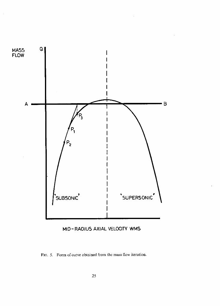
where Q is the required mass flow and Ri, R o are the inner and outer radii of the annulus*. This integral is evaluated using Simpson's rule to obtain a mass flow. The axial velocity at the mid-radius is adjusted and the flow conditions re-determined until the calculated mass flow is correct to within a tolerance of 0.1 per cent. Details of the alteration of the mid-radius axial velocity for this iteration are given in Appendix II and on Figure 5.

When convergence of this continuity iteration has been achieved, the mass flow or stream function distribution is known across the annulus.

2.2.2. Stream function. The above determination of the flow at each grid point on a plane is repeated for each calculating plane, except for the first and last two planes, to obtain a stream function distribution ~ throughout the flow field on the nth overall iteration. For an iterative process, numerical stability can be a problem and this was overcome by the introduction of a relaxation factor r f . A new stream function for the nth iteration is defined by

The solution of the principal equations is obtained by iterating on the stream function distribution until a specified number of iterations has been completed.

2.3. Evaluation o f Terms in Principal Equations.

*If account is taken of the annulus wall boundary layer, then Ri, Ro will be the adjusted values to allow for the boundary layer displacement thickness.

5

d2r In equation (1), tan 2 and d-z~ are calculated from the streamline pattern. At each grid point, they

are the first and second derivatives of the streamline through that point projected onto a radial plane and are evaluated by fitting a cubic spine through the grid point and the positions on the two previous and two subsequent calculating planes for which the stream function is the same as at the grid point being considered. Each position is found by a linear interpolation of the stream function distribution.

O(tan22) is calculated from the distribution of tan 2 by means of a quadratic fit. The term ½ (?r

dB The term dzz is evaluated from the identity (A17a) in Appendix I, c~B c~B ~z and ~rr being found by using

(rVo) a quadratic fit. In the same way, the term ~ z z is evaluated with rVo replacing B in identity (A17a)

in Appendix 1, the distribution of rVo being taken from the previous iteration. For the first iteration,

d(rVo) is taken to be zero throughout the flow field. dz To evaluate Mz and tan ~, a knowledge of the stagnation enthalpy and the absolute swirl velocity is

required. This is obtained by the methods outlined in Sections 2.3.1 and 2.3.2. The entropy term in equation (3) is calculated as indicated in Section 2.3.3.

2.3.1. Calculation qfabsolute swirl velocity. Referring to Figure 6(a), if the streamline A C lies in a duct, then angular momentum is conserved from A to C

(rVo)a (Vo)c =

(r)c

If C lies within a blade row, then the flow is made to follow the prescribed stream surface. Combining equations (A7), (A18a) and (A18b) from Appendix I, then

Wo = - Wr tan 2 ' - W~ tan # ' ,

which is the geometrical condition that the flow should follow the mean stream surface. Applying this equation at C, we get, within a stator row

Vo = - Wr tan 2 ' - Wz tan/~'

and within a rotor

Vo = - Wr tan 2' - W z tan/~' + ~or.

The situation where A C cuts the trailing edge of a blade, as shown in Figure 6b, is a special case. It is necessary to find the angular momentum at F and then conserve angular momentum from F to C. To enable this to be done, tan 2' and tan #' are prescribed at the trailing edge point F together with the position of F. Also, the density is used from the previous iteration (inlet static density for the first iteration) and the flow properties are assumed to vary linearly from A to C.

2.3.2. Calculation of stagnation enthalpy. Referring to Figure 6, i f A C lies in a duct or within a stator row, then stagnation enthalpy is conserved from A to C.

H c -~- H A .

6

I f A C lies within a rotor row, then rothalpy I = H - o ) r V o is conserved from A to C (see Appendix III)

H c = H A -'k 09 c [(rVo) c - (rVo)A] .

Any other case can be considered as a combination of these two.

2.3.3. Calculation o f entropy. Losses are simulated by prescribing distributions, throughout the flow field, of two local polytropic efficiencies.

t h i s r qc = ~ Ior compression

and Ah

t/r = -ZT--, for expansion, ani~

where Aha is the change in enthalpy for an isentropic process having the same initial state as the actual process.

Therefore, the changes of entropy and enthalpy are related, thus

and

, f T + A T ~ As = Cp (1 -qc ) ' o g e e s )

/T+AT .T/'°ge T-Y-)

3. Numer ica l Examples .

Two numerical examples are given to il lustratethe use of the computer program. The first example is a two-stage, highly loaded, axial flow turbine s and the second is a low pressure ratio, single-stage, axial flow compressor 9.

As mentioned earlier, there are two alternative methods for analysing the meridional flow pattern, known as the Matrix Through-Flow and the Streamline Curvature Duct Flow methods. Both of these methods have been applied to the above turbomachines and compared with the method, known as the Streamline Curvature Through-Flow, developed in this Report.

In all the above methods, irreversibility is introduced by the specification of a local polytropic efficiency for expansion and one for compression at each grid point. For the turbine, the two efficiencies were assumed to be equal and constant throughout the flow field, and were selected such that, for the chosen mass flow and rotational speed, the predicted overall pressure ratio was in agreement with the experi- mental value. In the case of the compressor, a value of 90 per cent was chosen for the two efficiencies at all grid points.

The assumptions regarding the shape of the mean stream surface were that the value of tan p' varied linearly between the design inlet and outlet values, and that

circumferential blade thickness B =

blade pitch

3.1. Two-S tage Turbine.

This turbine, having an overall loading of 3.25 for the two stages, was fitted with aerofoil camber-line type blading. The base profile shape was placed around a parabolic camber line with the position of maximum camber at 40 per cent of the chord from the leading edge. In selecting the blade pitch/chord ratio, the loading criterion t°, expressed as the ratio of tangential lift experienced by the blade to the

exit dynamic head, was adopted and limited to the range 0-7 to 1-1. The annulus was flared, with hub/tip ratio falling more or less linearly from 0.8 at inlet to the first-stage stator to 0.66 at exit from the second- stage rotor. An unusual feature of this machine is the 10 degree radial tilt on the second-stage stator blades, that of the other blade rows being negligible.

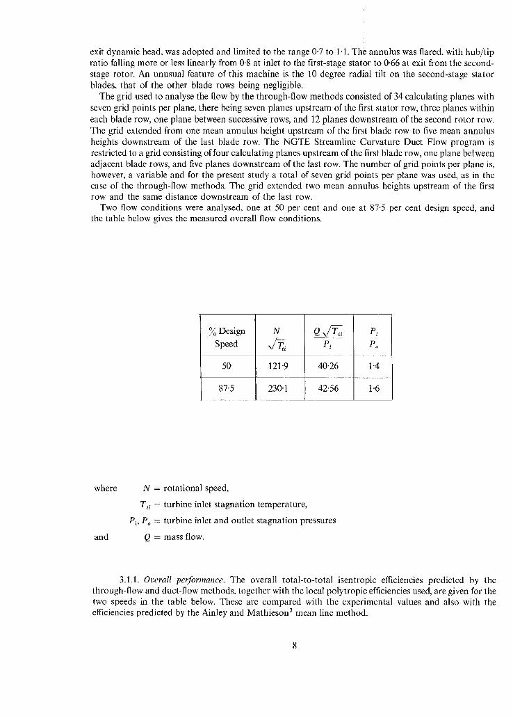
The grid used to analyse the flow by the through-flow methods consisted of 34 calculating planes with seven grid points per plane, there being seven planes upstream of the first stator row, three planes within each blade row, one plane between successive rows, and 12 planes downstream of the second rotor row. The grid extended from one mean annulus height upstream of the first blade row to five mean annulus heights downstream of the last blade row. The NGTE Streamline Curvature Duct Flow program is restricted to a grid consisting of four calculating planes upstream of the first blade row, one plane between adjacent blade rows, and five planes downstream of the last row. The number of grid points per plane is, however, a variable and for the present study a total of seven grid points per plane was used, as in the case of the through-flow methods. The grid extended two mean annulus heights upstream of the first row and the same distance downstream of the last row.

Two flow conditions were analysed, one at 50 per cent and one at 87-5 per cent design speed, and the table below gives the measured overall flow conditions.

Design

Speed

N Pi

Po e i

50 121"9 40.26 1'4

87"5 230-1 42.56 1"6

where

and

N = rotational speed,

T,~ = turbine inlet stagnation temperature,

P~, Po = turbine inlet and outlet stagnation pressures

Q = mass flow.

3.1.1. Overall performance. The overall total-to-total isentropic efficiencies predicted by the through-flow and duct-flow methods, together with the local polytropic efficiencies used, are given for the two speeds in the table below. These are compared with the experimental values and also with the efficiencies predicted by the Ainley and Mathieson 3 mean line method.

Streamline Curvature Matrix

Through Flow Through Duct

Flow Flow

94 87

89.8 86-1

98.5 92

97-8 92.2

Ainley and

Mathieson Experi- ment

Design Speed

Local polytropic efficiency ~ 94

50 Overall isentropic efficiency 9/0 89.8 80"8 81.5

Local polytropic efficiency ~ 97.5

87.5 Overall isentropic efficiency ~ 96.2 85'3 86.5

It can be seen that the efficiencies given by the simple mean line method agree well with experiment, the maximum discrepancy being only 1.2 per cent. The predictions of the three advanced methods under consideration are all far too high, the Streamling Curvature Duct Flow method being rather better than the through-flow methods. The through-flow methods are, however, in very close agreement with each other, as is to be expected since they make precisely the same assumptions. The poor predictions of the through-flow and duct flow methods are obviously due to the high levels of local polytropic efficiency needed to obtain the correct pressure ratio and it is probable that this in turn is due to the assumption of a constant polytropic efficiency throughout the flow field. The effects of this assumption seem to be magnified by calculating the flow within the blade rows. These predictions of the overall performance show clearly the need for a better model for the representation and distribution of flow losses.

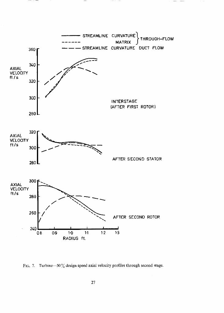
3.1.2. Flow profiles. Figures 7 and 8 show comparisons of the axial velocity profiles predicted by the through-flow and duct flow methods through the second stage, there being greater differences between the results in this area of the turbine than in the first stage. The results obtained from the through-flow methods are in excellent agreement but differ considerably from those of the duct flow method, except after the second stator. This, however, must be viewed in the context of the changing profile through the second stage, that is, it is coincidence that the profiles after the second stator are similar for the two speeds.

The theoretical and experimental profiles of axial velocity and swirl angle far downstream of the second-stage rotor row are shown in Figures 9 and 10. Once again, the through-flow methods are in very close agreement with each other and give a reasonable estimate of the axial velocity profile, parti- cularly for the 50 per cent design speed point. The simple duct flow method yields a radial variation of both axial velocity and swirl angle quite different to the through-flow predictions and that found experi- mentally. The lack of agreement between the through flow predictions and experimental results near the walls would appear to be due to the unrealistic distribution of loss, causing the axial velocities to increase, rather than decrease, towards the walls. This once again shows the need for a better loss model.

3.1.3. Annulus wall static pressure distributions. Experiment indicated a radial static pressure gradient at outlet from the first stage in the opposite sense to that normally expected for swirling flow in an annulus: the wall static pressure measured at the hub was higher than that measured at the casing. It is thought that this is probably due to the radial tilt of the second-stage stator blades, which is much greater than is normally encountered in axial flow machines, inducing a strong radial acceleration of the flow.

The distributions of wall static pressures obtained from the Streamline Curvature Through-Flow and Duct Flow methods, non-dimensionalised by the inlet stagnation pressure, are compared with experi- mental data in Figures 11 and 12. The static pressures obtained from the Matrix Through-Flow method are not shown since they were nearly identical to those given by the Streamline Curvature Through-Flow method. The inverse pressure gradient was successfully reproduced by the through-flow methods whereas the duct flow approach predicted practically no pressure gradient at all, for both speeds.

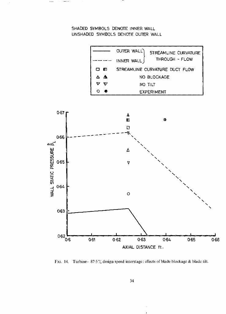
3.1.4. Effects of blade blockage and radial tilt. As has been pointed out earlier, the results obtained from the Streamline Curvature Duct Flow method differ markedly from the through-flow methods. This difference must be attributed to the extra assumptions implied by the absence of computation inside the blade rows in the duct flow model, namely, the neglect of blade blockage and radial tilt effects. To investigate this further, two special cases were analysed using the Streamline Curvature Through-Flow method, for the flow condition at 87-5 per cent design speed, firstly neglecting only blade blockage and, secondly, neglecting only radial tilt. For the two cases, the same procedure was adopted for fixing the loss distribution as had been used for the previous calculations. A common value for the local polytropic efficiencies of compression and expansion was chosen, which was constant throughout the flow field, such that the predicted overall pressure ratio agreed with the experimental value.

The local polytropic efficiency for the case with no blade tilt was 98.5 per cent. Thus, it may be seen from the table of efficiencies given earlier in Section 3.1.1 that neglecting the blade tilt did not alter the overall pressure ratio. It did, however, alter the shape of the axial velocity and swirl angle profiles and this is reflected in the comparison of the far downstream flow profiles given in Figure 13. In fact, the profiles obtained are very close to those given by the Streamline Curvature Duct Flow method.

The value of local polytropic efficiency used for the case with no blade blockage was 90 per cent. The resulting far downstream axial velocity and swirl angle profiles, Figure 13, show that the effect of blade blockage is significant but far less so than blade tilt.

A comparison of the wall static pressures at the interstage of the turbine is given in Figure 14. It can be seen that removal of the blade blockage and removal of the radial tilt both have the effect of reducing the inverse static pressure gradient.

3.2. Single-Stage Compressor. This compressor 9, having a constant hub/tip diameter ratio of 0-5, had inlet guide vanes, a rotor row

and a stator row. The blading was designed for radially constant axial velocity and temperature rise, and stator inlet angle. The rotor row was approximately 50 per cent reaction at the mean diameter, where the relative air outlet angles were 25.6 degrees and the pitch/chord ratio was 0.9. The blade profiles were of C5/C50 aerofoil section with constant chord of 2 in., giving an aspect ratio of 2.5.

Analysis of the flow by the through-flow methods was carried out with eight calculating planes up- stream of the inlet guide vanes, three within each blade row, three between each pair of blade rows and 11 downstream of the stator row. The first plane of the grid was placed at 1.5 annulus heights ahead of the first blade row and the last plane 2-5 annulus heights downstream of the last row. A total of seven grid points were taken on each plane.

For the Streamline' Curvature Duct Flow method, the positioning of the calculating planes is subject to the requirements of the program, as was stated in the description of the grid for the two-stage turbine. There were again seven grid points per plane and the extent of the grid considered was the same as that used for the through-flow methods. The comparison between the theoretical predictions and experiment is made for one flow coefficient of 0.65. The flow coefficient is defined as the ratio of the mean axial velocity to blade rotational speed at mean diameter.

3.2.1. Results. The overall pressure ratio of this compressor was approximately 1.0035 for the flow condition considered. The usual procedure of lining up the predictions of pressure ratio with the experi- mental value, as applied to the turbine example, was found to be impractical since a large change of local polytropic efficiency produced only a very small change in the predicted pressure ratio. However, to

10

allow for the effect of irreversibility, the flow pattern was calculated using an arbitrary value of 90 per cent for the polytropic efficiency of compression and expansion at all grid points in all three analytical methods, as stated in Section 3.

The experimental and predicted profiles of axial velocity, far downstream of the stator row, are com- pared in Figure 15. It will be observed that, ignoring end wall boundary layer effects, the through-flow methods, which are in close agreement with each other, give a fair estimate of the velocity profile. The simpler Streamline Curvature Duct Flow method leads to a radial variation of axial velocity which is quite different to that given by the through-flow methods and this must be due entirely to the neglect of blade thickness effects since there is no radial tilt of the blades.

4. Conclusions.

A Streamline Curvature Duct Flow computer program for analysing the flow through turbomachines but which only allows flow calculations in the duct regions has been extended so that the flow may also be calculated within the blade rows. This has been done by using the concept of a meridional stream surface of specified shape and thickness. This model of the flow is known as the Streamline Curvature Through-Flow method.

Two turbomachines have been selected as test cases for the program: a two-stage turbine and a low pressure ratio, single-stage compressor.

The program predictions have been compared with experimental data and with results from the Matrix Through-Flow and Streamline Curvature Duct Flow methods.

Very good agreement has been obtained between the Matrix and Streamline Curvature Through- Flow programs. One advantage of the Streamline Curvature Through-Flow approach over the Matrix method is that it does not require a computer having a large high speed store. The program described in this Report might take up a store of 21K on an SDS 90/300 computer, which has a 24 bit word, whereas to analyse the same problem using the Matrix Through-Flow program would require a store of 21K on a KDF9 computer, which has a 48 bit word. The corresponding run times would be 15 minutes per case for the Streamline Curvature program and 10 minutes per flow condition after an initial 5 minutes for a particular geometry using the Matrix program. These figures are only meant to be approximate.

A comparison between the Streamline Curvature Duct Flow program and the new Streamline Curva- ture Through-Flow program indicates that both of the two main effects neglected by the duct flow model, ie, blade blockage and blade radial tilt effects, are significant when looking at the detailed flow through a turbomachine.

The comparisons with experiment show that the through-flow methods give a reasonable estimate of the axial velocity and swirl angle profiles. An improvement on the measure of agreement calls for a better model for the representation and distribution of flow losses. However, by making use of a simple loss distribution, the accuracy of calculating annulus wall static pressure distributions, for example, is significantly better when the through-flow methods are used, when compared to the simple Streamline Curvature Duct Flow method.

N O T E

Advice on the use of this program together with a copy of a Note 11 on the preparation of the data can be obtained on application to the National Gas Turbine Establishment. Punched paper tape versions of the program are also available.

11

B

Cp

F

h

H

M

n

P

P i

O r, O, Z

s

T

V

W

2

2' ,p'

P

6O

Superscript

i}r ' ¢?z

N O T A T I O N

Mean stream surface thickness parameter

Specific heat at constant pressure

Force vector

Static enthalpy per unit mass

Stagnation enthalpy per unit mass

Mach number

Vector normal to the mean stream surface

Static pressure

Inlet stagnation pressure

Mass flow

Radial, circumferential and axial co-ordinates

Entropy per unit mass

Static temperature

Absolute velocity vector

Relative velocity vector

Absolute swirl angle

Meridional angle

Angles which define the local shape of the mean stream surface

Static density

Angular velocity of the blade

Derivatives taken along the mean stream surface

12

No. Author(s) 1 A.R. Howell . . . .

2 A.R. Howell . . . .

3 D .G . Ainley and G. C. R. Mathieson

4 R.A. Novak ..

5 L .H . Smith . . . . . .

6 M.E. Silvesterand .. R. Hetherington

7 H. Marsh . . . . . .

8 I .H. Johnston and D. E. Smart

9 R.A. Jeffs . . . . . .

10 D.J .L . Smith, I. H. Johnston and D. J. Fullbrook . . . .

11 D .H . Frost . . . . . .

LIST OF REFERENCES

Title, etc. •. Fluid dynamics of axial compressors.

Proc. Instn. Mech. Engrs., Vol. 153, p. 441, (1945).

•. Design of axial flow compressors. Proc. Instn. Mech. Engrs., Vol. 153, p. 452, (1945).

•. A method of performance estimation for axial flow turbines. A.R.C.R. & M. 2974, (1951).

. . Streamline curvature computing procedures for fluid flow problems.

J. Eng. Power, Trans. ASME, Series A, Vol. 89, 1967•

The radial equilibrium equation of turbomachinery J. Eng. Power, Trans. ASME, Series A, Vol. 88, 1966.

. . A numerical solution of the three-dimensional compressil~le flow through axial turbomachinery in Numerical Analys is--An Introduction•

Edited by J. Welsh, Academic Press, (1966).

A digital computer program for the through-flow fluid mechanics in an arbitrary turbomachine using a matrix method.

A.R.C.R. & M. 3509, (1966)•

An experiment in turbine blade profile design• A.R.C. CP No. 941, (1965).

The low speed performance of a single stage of twisted constant section blades at a diameter ratio of 0.5.

Unpublished MAS material.

Investigations on an experimental single-stage turbine of con- servative design. Part I A rational aerodynamic design procedure. Part II Test performance of design configuration. A.R.C.R. & M. 3541, (1967).

A Streamline Curvature Through-Flow computer program for analysing the flow through axial-flow turbomachines--

Note on data preparation. Unpublished MAS material•

13

APPENDIX I

Derivation of Principal Equations.

Since this work is apparently the first to introduce the concept of a meridional stream surface into the streamline curvature analysis, the derivation of the principal equations is given in some detail.

For a co-ordinate frame of reference rotating with a blade row at constant angular velocity co, the equation of motion for inviscid, steady flow is

1 (W_.V_) W_= - - V p + c o z E - 2 c o A W_

P

assuming gravitational forces are small. Using a relative cylindrical polar system (r, 0, z) such that the rotation is about the z-axis and 0 is

measured in the direction of rotation, the three component equations of motion are

Wo OWr 1 Op ~3W r OWr W°2 + 2coWo-coZr - , (A.1) W~ ~rr + Wz ~z r r O0 p Or

OW=_~ WoOW z 1 Op w~ + w = - s S r 0 0 - pOz

and WoOWo 1 Op

+ 2coWr - (A.3) r O0 pr O0"

The equation of continuity for steady flow is

g . (p_v¢) = 0,

which in scalar form becomes

1 O(prWr) 1 O(pWo) O(pW=) r Or + - - ~ - 0. (A.4) r 00 Oz

Also, from the first and second laws of thermodynamics

1 T V s = Vh - 2 Vp.

P

Therefore, TOS _ Oh 1 Op Or Or p Or" (A.5)

In general, equations (A.I) to (A.5) have no simple solution and must therefore be simplified in some way. In the streamline curvature method, this is effected by reducing the problem to two dimensions, as in the matrix through-flow method, by assuming a relationship 0 = O(r, z), taken to be single-valued in 0. That is, the solution is only obtained on a prescribed meridional surface S. Thus, any quantity q(r, O, z) in the original problem will now be r, z dependent only.

Let 0q and 0q be special partial derivatives where ~ will be the rate of change of q with r on the surface 0r ~z

14

S at a given value of z, and Oq will be the rate of change of q with z on the surface S at a given value of r. Oz

Consider the curve F defined by the intersection of the surface S and a plane z = constant, then

3q dq - o n F

Or dr

Oq Oq dO -

Or 90 dr

But n~ dr + no rdO = 0

on the curve F, where n~, no, n~ are the direction cosines of the normal to the prescribed surface. It follows, therefore, that

Similarly

Oq _ Oq 1 n~ Oq

Or Or r no 20

Oq _ Oq l n~ Oq

Oz Oz r no 20 "

(A.6)

If the prescribed meridional surface S is taken to be a stream surface, then

nr W~+no Wo+nz W~ = O. (A.7)

Expressing equations (A.1) to (A.5) in terms of the special derivatives equation (A.6), and making use of equation (A.7), we get

3W~ Wo z 1 Op 3Wr + Wz 2 o W o - co2r = F~ - - - - (A.8)

W~ Or Oz r p Or'

~ r ~ OW~ _ Fz 1 Op (A.9) +wz 0z

OWo OWo Wo W'--~-r + Wz-~-z + rWr + 2~°W~ = F°' (A.IO)

10(prWr) O(pWz) 1 [- OWN OWz OWo-] r Or ~ O ~ - rnoLnr-~-+nz-~o-+n°-~O-A (A.11)

Oh 0s 1 0p (A.12) and Or = T ~ r + p O--r'

where _F is a vector, having the unit of force per unit mass of gas, defined by

1 10p F - - nor p 20 n_.

15

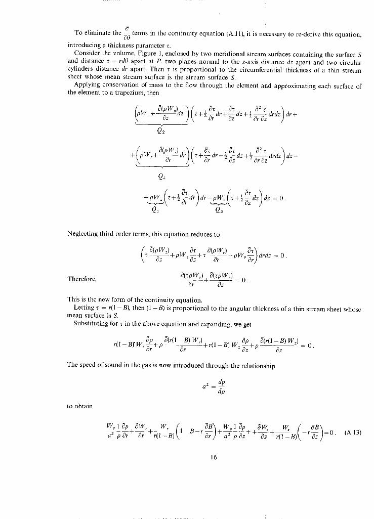
0 To eliminate the ~-0 terms in the continuity equation (A.11), it is necessary to re-derive this equation,

introducing a thickness parameter -c. Consider the volume, Figure 1, enclosed by two meridional stream surfaces containing the surface S

and distance ~: = rdO apart at P, two planes normal to the z-axis distance dz apart and two circular cylinders distance dr apart. Then r is proportional to the circumferential thickness of a thin stream sheet whose mean stream surface is the stream surface S.

Applying conservation of mass to the flow through the element and approximating each surface of the element to a trapezium, then

p ~(pW=). ) , e z + : O~zz drdz dr+

, t

Q~

+ PW~+-~r dr ~ + ~ r ~TzdZ+~O~zdrdz dz-

Q.4

W 1" 1~'c \dr-pW~('c+13"c \ - . - ,

Q1 Q3

Neglecting third order terms, this equation reduces to

Oz PW= ~z+ Z + pWr drdz = O.

Therefore, 0(~pW~) ÷ _ _ _ 0. ~3r cqz

This is the new form of the continuity equation. Letting z = r(1 -B) , then (1 - B ) is proportional to the angular thickness of a thin stream sheet whose

mean surface is S. Substituting for z in the above equation and expanding, we get

_BrW3P+p 3(r(1 - B ) W,.) r(l ~r 0r

~p 3(r(1 - B) W=) + r ( 1 - B ) W= ~z+p Oz - 0 .

The speed of sound in the gas is now introduced through the relationship

a 2 @ dp

to obtain

( OB) W=lOp 3W z VV= [" ~B) Wrl ~p OW, Wr -r~-r a 2 p~z aZ p ~ r + ~ r - r + ~ I - B -4 t - + ~ - z z + ~ ) ~ - r - ~ z z = 0 . (A.13)

16

Eliminating o-p from the axial equation of motion (A.9) and equation (A. 13) then Oz

Wrl Op t_OW~ +W, Wr OB _Wz( ~Wz OWz\ a 2 p~rr -&r r (1-----B)~r ~ - F~-Wr-&r - W ~ Z - z ) +

3W~ W_ 3B -F 0~ (1L-B) Oz = 0. (A.14)

Now, let u be the absolute swirl angle and 2 be the angle that the projection of the streamline on to the r, z plane makes with the axial direction.

Then V o = V~ tan c~.

Since Wo = Vo-mr, Wz = V~,

therefore Wo = Wz tan e - mr.

Similarly, Wr = W e tan 2.

Substituting these relationships into the radial equation of motion (A.8) and equation (A. 14) and el iminat- gw~ ~w~

ing 0 r ' ~z ' t hen

1 t~p _ i [Wz2 tan2 2 ÷ Wz2tan2~(1-Mz 2) p 0r (1 - M z 2 s e c 2 ).) r r

+ Wz 2 Mz 2 tan 2 - 0(tan 2) Wz 2 t a n 2/" OB + OB~

-- Wz 2 (1-- MzZ) ~ + Mz 2 tan 2 Fz+(1 - Mz 2) Ft. (A.15)

This equation can be simplified by the introduction of total derivatives. For any quantity q, using the equations (A.6),

~rr Oq l n~ Oq dr 3q l nr Oq ~ + t a n 2 =Oz rnoOO~-dz Or rno

Oq 10q/" dr dO'~ 0z In' Vz +nz+'°

dq (A.16) dz

20B_F 8B dB (A. 17a) Therefore, tan -&r ~ z - dz

17

and (A.17b) 2 0(tan 2)_ t 3(tan 2) d(tan 2) dZr

tan ~ 0 ~ - dz - dz 2"

It is also necessary to obtain expressions for the force components Fr and Fz. If the geometry of the stream surface is defined by two angles 2' and/z' where 2' is the angle between

the stream surface and the radial direction in the r, 0 plane and/2' is the angle between the stream surface and the axial direction in the z, 0 plane, as shown in Figure 2, then

tan 2' = r/r - Fr no Fo (A. 18 a)

and tan# ' - nz _ Fz no Fo

Using the relationship (A.18a) with equation (A.10), then

F r = ( W 3Wo _~r +Wz~_z WorWr+2o)Wr)tan2,

(wr~(rVo) w~ ~(rVo)'~ 2' - Or + 7 Oz ]tan .

Therefore, making use of equation (A.16),

W z d(r Vo) Fr - tan 2'.

r dz Similarly, using equations (A.18b) and (A.10), then

(A.19a)

F~ _ __Wzr ~ tan p' . (A.19b)

Substituting from equations (A. 17a), (A. 17b), (A. 19a), (A. 19b) into equation (A.15), we get

l o p _ W~ z ItanrZ2 0(tan22)+(1 2 ftanZc~ d 2 r } ] p Or (1-M~ 2 see 2 2) +½ O ~ - M z ) ~ r dz 2 -

Wz 2 tan 2 1 dB (I - M z 2 see 2 2) (1 - B ) d z +

E '1 + (1 - M z a) tan 2 '+Mz a tan 2 tan #' Wz_ d(rVo) r dz (A.20)

Equations (A.12) and (A.20) are the principal equations to be solved. In this analysis, it has been assumed that the equations are not time dependent, that is, that the flow

relative to each blade row is steady. However, the flow and gas state at exit from a blade row vary cir- cumferentially and the following blade row is then subject to a time dependent inlet flow. To overcome

dB this, the flow is assumed to be axisymmetric within the duct regions. This means that the terms dzz and

d(rVo) . dz in equation (A.20) will both be zero and thus, the mean stream surface need not be specified within

the duct regions.

18

APPENDIX II

Adjustment of Axial Velocity.

Axial velocity iteration--adjustment of W X . Two typical plots of W X vs W Y are shown in Figure 4. In both cases, the solution required is the lower intersection with the straight line W X = WY . The

1 other intersection points result from the term in equation (1) tending to infinity as Mz 2

1 - M z 2 sec 2 ~. sec 2 2, the meridional Mach number Mm, tends to unity, giving an asymptote as shown. This behaviour is clearly unrepresentative of the real flow and consequently, the solutions close to the asymptote are incorrect. For reasons of convergence, this restricts calculations to those problems for which the meri- dional Mach number is everywhere below unity.

Consider the axial velocity iteration which gives rise to the "high Mach number" curve. As a first guess, W X is taken to be equal to Wz(i,j). This value of W X with the value of W Y obtained from it, correspond to a point P~ representing the first iteration. For the second iteration, W X is made equal to W Y from the first iteration. Again, W Y is calculated, giving a point P2" The third value of W X is given by the intersection of the straight line P1 P2 and W X = W Y . Subsequent values of W X are given by the intersection of W X = W Y and the straight line through the point corresponding to the previous iteration and parallel to P1 P2.

Mass flow iteration--adjustment of mid-radius axial velocity. If W~ at the mid-point, denoted by W MS, is plotted against the calculated mass flow, a curve of the form shown in Figure 5 is obtained, where the line AB indicates the required flow. The left hand section of the curve, labelled 'subsonic', corres- ponds to solutions which are either wholly subsonic or partly subsonic and partly supersonic, while the right hand section of the curve, labelled 'supersonic', corresponds to solutions which are either wholly supersonic or partly supersonic and partly subsonic. The program is written to choose the value of W M S corresponding to the 'subsonic' solution.

The first iteration will produce a point Px. W M S for the second iteration is taken to be 97 per cent of the starting (first iteration) value of W M S and the mass flow re-calculated, giving the point P2. The value of W M S for the nth iteration is obtained by a linear interpolation from the values used for itera- tions (n-2) and (n-1). Thus for the third iteration, W M S is given by the intersection of P1 P2 and AB.

19

APPENDIX III

Conservat ion o f Rothalpy .

For a frame of reference rotating with a blade row at constant angular velocity co, the equation of motion for inviscid, steady flow can be written in the form

WA (_VA _g0-2oaA _LW= V I - T V s , (A.21)

where I is the quantity rothalpy defined as

I = H - oar V o

and gravitational forces have been neglected. Forming the inner product of equation (A.21) with the relative velocity vector _W, we obtain

_W. V I - r W. Vs = 0. (A.22)

As in a stationary frame, entropy will be conserved along streamlines.

Thus,

Therefore, using equation (A.22),

W_ . V s = O .

_w.vi=o,

which implies that rothalpy is conserved along streamlines for steady flow in a rotating frame.

20

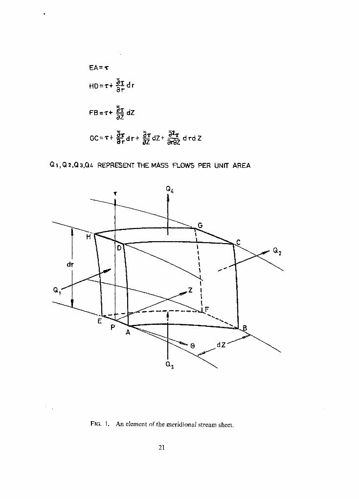
EA=¢

HD=~'+ ~rdr

FB "- -r+ }~ dz

GC=¢+ ~-rdr+ ~ dZ+ a~z d~-d Z

Q 1, Q 2,Q 3,QA REPRESENT THE MASS FLOWS PER UNIT AREA

Q¢

Q

dr

D

P

Ct 3

| | | I I

-4. I I

e

0. 2

1..-dz

FIo. 1. An element of the meridional stream sheet.

21

~' -I-1J e Z

• 0

COMPRESSOR STAGE

03,Q

J.' + a o g

Z TURBINE STAGE

, r

~f_ HUB

TIP

FIG. 2. Mean stream surface angles 2' and #'.

22

;:z>

=_., J=2

J=l

J f

f

UPSTREAM BOUNDARY

i.=1 L=2

r

.___~ AXIS OF ROTATION

STATOR ROTOR

DOWNSTREAM BOUNDARY

L= N-I L=N

+ REQUIRED SOLUTION

WY

ASYMPTOTE (Mm.- 1)

HIGH MACH. No

LOW MACH .No.

P~

W ×

FIG. 4. Forms of curve obtained from the velocity iteration.

24

MASS FLOW

A

Q

Ii

SUBSONIC P

SUPERSONIC

B

MID-RADIUS AXIAL VELOCITY WMS

FIG. 5. Form of curve obtained from the mass flow iteration.

25

( [ -~ j )

STREAMLINE

/ C(i , , J )

(a) THE STREAMLINE A C

TRAILING EDGE

O ~-------~-"-~C( L~ J ) ( i - l , J ) I ~ . / F I

A

F

(b) STREAMLINE AND TRAILING EDGE

FIG. 6. Streamline intercepts.

26

AXIAL VELOCITY ft Is

STREAMLINE CURVA,rURE'~t THROUGH-FLOW MATRIX J

360 - STREAMLINE CURVATURE DUCT FLOW

340 / ~

320

300 INTERS'rAGE (AFTER FIRST ROTOR}

280

320 AXIAL VELOCITY f t /s

3O0

280 AFTER SECOND STATOR

AXIAL 300 VELOCITY ft / s 280

/ 260 /

240 I 08 0.9

I I I 1"0 1.1 1'2

RADIUS ft.

AFTER SECOND ROTOR

I 1'3

FIG. 7. Turbine--50 ~ design speed axial velocity profiles through second stage.

2?

AXIAL VELOC I1 Y

f t l S

420

400

380

360

340

" x

STREAM LI NE CURVATURE/ MATRIX P j THROUGH - FLOW

STREAMLINE CURVATURE DUCT FLOW

/ ~ ~ I NTERSTAGE (AFTER FIRST ROTOR )

AXIAL VELOCITY

f t l S

380

360

340

>,

f /

AFTER SECOND STATOR

AXIAL VELOCITY

f t /S

360

340

320

300

280 0-~

/ /

/

"-- . . . . . . . . w ~ . ,~' '~" . / /

/ /

f AFTER SECOND ROTOR

. . . . . . . . . . . . . . J . . . . . . . . . . . . . . . 1 . . . . . . . . . . . . . . . . . . _ 1 . . . . . . . . . . . . . . . . . _ l . . . . . . . . . . . . . . J

0.9 1.0 1.1 1.2 1-3

RADIUS f t .

FIG. 8. Turbine--87.5 ~o design speed axial velocity profiles through second stage.

28

320

300

240

280 AXIAL VELOCITY f t / s

260

220

15

10

5

STREAMLINE CURVATURE~ MATRIX j THROUGH- FLOW

STREAMLINE CURVATURE DUCT FLOW '~ o EXPERIMENT

\ "% o ° ~ , ° o /

o /

/ f X ~ .

o

o

o

SWIRL ANGLE DEGREES

340

0 0 0 0

0 0

-5 i 1 I I I

0"8 0"9 1'0 1'1 1'2 1"3 RADIUS ft.

FIG. 9. Turbine--50 ~ design speed far downstream flow profiles.

29

400 O

STREAMLINE CURVATURE~ MATRIX J THROUGH FLOW

STREAMLINE CURVATURE DUCT FLOW EXPERIMENT

380 / /

360 / / AXIAL /~/

300

281

o

SWIRL ANGLE DEGREES

3 5 '

3O o o

25 . ,s

20 .,,~,,~ 0"8

_o.

/ o o - ~ o

o o o

0"9 1"0 1-1 1'2 1-3 RADIUS ft

FIG. 10. Turbine--87.5 % design speed far downstream flow profiles.

30

,o~

0'9

0,8 ° ..,,,D

" 1 1 3 .

t.U rr 23 d')

0.7 i i i r r

o. (J

. 0"6 - J

0"5

0.4

0-3 0"3

OUTER WALL| STREAMLINE CURVATURE

]1~ THROUGH - FLOW INNER WALL

WALL'I, STREAMLINE CURVATURE [3 OUTER II INNER WALL ~.) DUCT FLOW

~ " .. 0 OUTER WALL'~ I \ ' ~ ~ EXPERIMENT [I ~ • INNER WALL.)

-

,, , - , ,_~. --..__. ~ ~\ / I I / / I " - . . / t - -

/ % /

/

I I I I I I 0"4 0.5 0,6 0.7 0-8 0.9

AXIAL DISTANCE ft

FIG. 11. Turbine--50 ~ design speed comparison of static pressures.

31

1.0

0.9

0'8

. . , J

"~ I O .

u J r r 5 3 et3 ,,n 0.7 LLI nr" O .

U

, 0"6 _.1

0"5

0"4.

0.3 0"3

OUTER WALL'] STREAMLINE CURVATURE

INNER WALLJ ~ THROUGH - FLOW

i 13 OUTERWALL~ t STREAMLINE CURVATURE m INNER WALL.) DUCT FLOW

-. O OUTER WALL'] ~ EXPERIMENT

® INNER WALL J

m

~ n

m

~, ® r-\--s, ', ,.. / k__Q'.

/ "-../" \ ",~. n / ,,

A / \ / V " ~ / /

I II J I . . . . . . . . I _ I

0-4 0.5 0'6 0.7 0"8 0'9

AXIAL DISTANCE f t .

FIG. 12. Turbine--87.5 % design speed comparison of static pressures.

32

AXIAL VELOCITY f t / s

400

STREAMLINE CURVATURE THROUGH FLOW STREAMLINE CURVATURE DUCT FLOW

NO BLOCKAGE NO TILT

380 /, /') // ' /

3o0 ~ ,/~//

320

300

280

J

SWIRL ANGLE DEGREES

35

30

25

20 I I I I I 0'8 0-9 1"0 1.1 1.2 1.3

RADIUS f t .

FIG. 13. Turbine---87"5 ~o design speed-far downstream effects of blade blockage & blade tilt.

33

SHADED SYMBOLS DENOTE INNER WALL UNSHADED SYMBOLS DENOTE OUTER WALL

[] 8

A

O ®

OUTER WALL 7 STREAMLINE CURVATURE

INNER WALL J f THROUGH - FLOW

STREAMLINE CURVATURE DUCT FLOW

NO BLOCKAGE

NO TILT

EXPERIMENT

0"67

0'66

-~IQ=

W

03 03 w 0.65 re" EL

(.3

~ 0 .64 . J

063

0'62 0.6

A m

[]

A

7

@

\ \

\ \

\ \

\ \

\ \ .

\

\ \

O \ \

\ \

\

. . . . . . . . . . . . . ___L__ . . . . _ _ _ . _ , _ _ . _ . _ _ . _ , _ _ . _ ' ...................... 1 . . . . . . . . . . . . . . . . . . J_ . . . . . . . . . . . . . . . . 1

0"61 0-62 0-63 0"6/+ 0.65 0"66

AXIAL DISTANCE ft.

F~G. 14. Turbine--87"5 ~o design speed interstage" effects of blade blockage & blade tilt.

34

STREAMLINE CURVATURE" L - MATRIX j THROUGH- FLOW

- - - - - - STREAMLINE CURVATURE DUCT FLOW O EXPERIMENT

AXIAL VELOCITY f t I s

70

65

60

55

50

45

\ \ \ / \ /

\ o o o / . ~ - /

o

I I I I 0-4 0"5 0"6 0"7 0.8

RADIUS ft.

I 0"9

FIc. 15. Compressor-comparison of far downstream axial velocity profiles.

Printed in Wales for Her Majesty's Stationery Office by Allens Printers (Wales) Limited

Dd. 502110 K.5 5/72

35

R. & M. NOo 3687

© Crown copyright 1972

HER MAJESTY'S STATIONERY OFFICE Government Bookshops

49 High Holborn, London WCIV 6HB 13a Castle Street, Edinburgh EH2 3AR

109 St Mary Street. CardiffCF1 IJW Brazennose Street, Manchester M60 8AS

50 Fairfax Street, Bristol BSI 3DE 258 Broad Street, Birmingham BI 2HE 80 Chichester Street, Belfast BT1 4JY

Government publications are also available through booksellers

R° & ~/L Noo 3687 SBN 11 470487 2