a stochastic optimal control perspective on a ect
TRANSCRIPT

UNIVERSITY OF CALIFORNIA, SAN DIEGO
A Stochastic Optimal Control Perspective on Affect-Sensitive Teaching
A dissertation submitted in partial satisfaction of the
requirements for the degree
Doctor of Philosophy
in
Computer Science
by
Jacob Richard Whitehill
Committee in charge:
Garrison Cottrell, ChairSerge BelongieAndrea ChibaJavier MovellanHarold PashlerLawrence SaulDavid Weber
2012

Copyright
Jacob Richard Whitehill, 2012
All rights reserved.

The dissertation of Jacob Richard Whitehill is approved,
and it is acceptable in quality and form for publication
on microfilm and electronically:
Chair
University of California, San Diego
2012
iii

DEDICATION
To Ms. Kenia Milloy and her 2011 Preuss School advisory students,
for whom I served as a math tutor for four years, and who lifted my
spirits during graduate school.
iv
TABLE OF CONTENTS
Signature Page . . . . . . . . . . . . . . . . . . . . . . . . . . . . . . . . . . iii
Dedication . . . . . . . . . . . . . . . . . . . . . . . . . . . . . . . . . . . . . iv
Table of Contents . . . . . . . . . . . . . . . . . . . . . . . . . . . . . . . . . v
List of Figures . . . . . . . . . . . . . . . . . . . . . . . . . . . . . . . . . . ix
List of Tables . . . . . . . . . . . . . . . . . . . . . . . . . . . . . . . . . . . xii
Acknowledgements . . . . . . . . . . . . . . . . . . . . . . . . . . . . . . . . xiii
Vita . . . . . . . . . . . . . . . . . . . . . . . . . . . . . . . . . . . . . . . . xv
Abstract of the Dissertation . . . . . . . . . . . . . . . . . . . . . . . . . . . xvii
Chapter 1 Introduction . . . . . . . . . . . . . . . . . . . . . . . . . . . . 11.1 Historical perspective . . . . . . . . . . . . . . . . . . . . 51.2 Notation . . . . . . . . . . . . . . . . . . . . . . . . . . . 61.3 Bayesian probabilistic reasoning . . . . . . . . . . . . . . 6
1.3.1 Bayesian belief updates . . . . . . . . . . . . . . . 71.4 Teaching as an Optimal Control Problem . . . . . . . . . 11
1.4.1 Immediate reward/costs . . . . . . . . . . . . . . 131.4.2 Belief . . . . . . . . . . . . . . . . . . . . . . . . . 141.4.3 Graphical model . . . . . . . . . . . . . . . . . . . 141.4.4 Belief updates . . . . . . . . . . . . . . . . . . . . 151.4.5 Control policy . . . . . . . . . . . . . . . . . . . . 161.4.6 Partially Observable Markov Decision Processes . 17
1.5 Affect-sensitive teaching . . . . . . . . . . . . . . . . . . 191.5.1 Affective and cognitive transition dynamics . . . . 201.5.2 Affective and cognitive observation likelihood . . . 211.5.3 Belief updates using affective observations . . . . 221.5.4 Designing affect-sensitive teachers . . . . . . . . . 22
1.6 Dissertation outline and contributions . . . . . . . . . . . 23
Chapter 2 Measuring the Benefit of Affective Sensors . . . . . . . . . . . 262.1 Introduction . . . . . . . . . . . . . . . . . . . . . . . . . 262.2 Related work . . . . . . . . . . . . . . . . . . . . . . . . 282.3 Cognitive skills training . . . . . . . . . . . . . . . . . . . 28
2.3.1 Human training versus computer training . . . . . 292.4 Experiment . . . . . . . . . . . . . . . . . . . . . . . . . 30
2.4.1 Conditions . . . . . . . . . . . . . . . . . . . . . . 32
v

2.4.2 Subjects . . . . . . . . . . . . . . . . . . . . . . . 342.5 Experimental results . . . . . . . . . . . . . . . . . . . . 35
2.5.1 Learning conditions . . . . . . . . . . . . . . . . . 352.5.2 Facial expression analysis . . . . . . . . . . . . . . 35
2.6 Towards an automated affect-sensitive teaching system . 372.7 Summary and further research . . . . . . . . . . . . . . . 382.8 Acknowledgement . . . . . . . . . . . . . . . . . . . . . . 39
Chapter 3 Automatic Recognition of Student Engagement . . . . . . . . 403.1 Introduction . . . . . . . . . . . . . . . . . . . . . . . . . 41
3.1.1 Recognizing student “engagement” . . . . . . . . 423.2 Related work . . . . . . . . . . . . . . . . . . . . . . . . 433.3 Dataset collection and annotation for an automatic en-
gagement classifier . . . . . . . . . . . . . . . . . . . . . 453.3.1 Data annotation . . . . . . . . . . . . . . . . . . . 473.3.2 Engagement categories and instructions . . . . . . 493.3.3 Timescale . . . . . . . . . . . . . . . . . . . . . . 513.3.4 Static pixels versus dynamics . . . . . . . . . . . 52
3.4 Automatic recognition architectures . . . . . . . . . . . . 543.4.1 Binary classification . . . . . . . . . . . . . . . . . 553.4.2 Data selection . . . . . . . . . . . . . . . . . . . . 573.4.3 Cross-validation . . . . . . . . . . . . . . . . . . . 583.4.4 Accuracy metric . . . . . . . . . . . . . . . . . . . 583.4.5 Hyperparameter selection . . . . . . . . . . . . . . 593.4.6 Results: binary classification . . . . . . . . . . . . 593.4.7 Generalization to a different dataset . . . . . . . . 613.4.8 Regression . . . . . . . . . . . . . . . . . . . . . . 613.4.9 Results: regression . . . . . . . . . . . . . . . . . 61
3.5 Reverse-engineering the human labelers . . . . . . . . . . 623.6 Comparison to objective measurements . . . . . . . . . . 64
3.6.1 Test performance . . . . . . . . . . . . . . . . . . 643.6.2 Learning . . . . . . . . . . . . . . . . . . . . . . . 66
3.7 Error analysis . . . . . . . . . . . . . . . . . . . . . . . . 663.8 Conclusion . . . . . . . . . . . . . . . . . . . . . . . . . . 683.9 Appendix: calculating inter-human accuracy . . . . . . . 683.10 Acknowledgments . . . . . . . . . . . . . . . . . . . . . . 69
Chapter 4 Measuring the Perceived Difficulty of a Lecture Using Auto-matic Facial Expression Recognition . . . . . . . . . . . . . . . 704.1 Introduction . . . . . . . . . . . . . . . . . . . . . . . . . 714.2 Facial Expression Recognition . . . . . . . . . . . . . . . 72
4.2.1 FACS . . . . . . . . . . . . . . . . . . . . . . . . 724.2.2 Automatic Facial Expression Recognition . . . . . 73
vi

4.3 Experiment . . . . . . . . . . . . . . . . . . . . . . . . . 734.3.1 Procedure . . . . . . . . . . . . . . . . . . . . . . 744.3.2 Human Subjects . . . . . . . . . . . . . . . . . . . 764.3.3 Data Collection and Processing . . . . . . . . . . 76
4.4 Results . . . . . . . . . . . . . . . . . . . . . . . . . . . . 774.4.1 Predicting Difficulty from Expression Data . . . . 794.4.2 Learning to Predict . . . . . . . . . . . . . . . . . 79
4.5 Conclusions . . . . . . . . . . . . . . . . . . . . . . . . . 814.6 Acknowledgement . . . . . . . . . . . . . . . . . . . . . . 82
Chapter 5 Teaching Word Meanings from Visual Examples . . . . . . . . 835.1 Introduction . . . . . . . . . . . . . . . . . . . . . . . . . 84
5.1.1 Contributions . . . . . . . . . . . . . . . . . . . . 855.1.2 Notation . . . . . . . . . . . . . . . . . . . . . . . 87
5.2 Related work . . . . . . . . . . . . . . . . . . . . . . . . 875.3 Learning setting . . . . . . . . . . . . . . . . . . . . . . . 895.4 POMDPs . . . . . . . . . . . . . . . . . . . . . . . . . . 925.5 Modeling the student as a Bayesian learner . . . . . . . . 93
5.5.1 Inference . . . . . . . . . . . . . . . . . . . . . . . 955.5.2 Adding noise . . . . . . . . . . . . . . . . . . . . 985.5.3 Dynamics model . . . . . . . . . . . . . . . . . . 1005.5.4 Observation model . . . . . . . . . . . . . . . . . 101
5.6 Teacher model . . . . . . . . . . . . . . . . . . . . . . . . 1045.6.1 Representing and updating Bt . . . . . . . . . . . 106
5.7 Computing a policy . . . . . . . . . . . . . . . . . . . . . 1075.7.1 Macro-controller . . . . . . . . . . . . . . . . . . . 1085.7.2 Micro-controller . . . . . . . . . . . . . . . . . . . 110
5.8 Procedure to train automatic teacher . . . . . . . . . . . 1105.9 Experiment . . . . . . . . . . . . . . . . . . . . . . . . . 111
5.9.1 How the OptimizedTeacher behaves . . . . . . . . 1135.9.2 RandomWordTeacher . . . . . . . . . . . . . . . . 1155.9.3 HandCraftedTeacher . . . . . . . . . . . . . . . . 1165.9.4 Experimental conditions . . . . . . . . . . . . . . 1175.9.5 Results . . . . . . . . . . . . . . . . . . . . . . . . 1175.9.6 Correlation between time and information gain . . 118
5.10 Incorporating affect . . . . . . . . . . . . . . . . . . . . . 1195.10.1 Simulation . . . . . . . . . . . . . . . . . . . . . . 120
5.11 Summary . . . . . . . . . . . . . . . . . . . . . . . . . . 1225.12 Appendix: Conditional independence proofs . . . . . . . 123
5.12.1 d-Separation of Wj from Wj′ for j′ 6= j . . . . . . 1235.12.2 d-Separation of Wj from Aνqν for all ν such that
qν 6= j . . . . . . . . . . . . . . . . . . . . . . . . 1245.13 Acknowledgement . . . . . . . . . . . . . . . . . . . . . . 124
vii

Bibliography . . . . . . . . . . . . . . . . . . . . . . . . . . . . . . . . . . . 126
viii
LIST OF FIGURES
Figure 1.1: Simple probabilistic graphical model representing whether Frankhas mastered the Pythagorean Theorem (S ∈ {unlearned, learned})and whether he answers a question about it correctly (O ∈{incorrect, correct}). . . . . . . . . . . . . . . . . . . . . . . . . 8
Figure 1.2: Graphical model of a POMDP. . . . . . . . . . . . . . . . . . . 15Figure 1.3: Optimal policy for the simple teaching example in Section 1.4. . 18Figure 1.4: POMDP to model affect-sensitive teaching. SKt is the student’s
“knowledge state”, SAt is the student’s “affective state”. . . . . 20Figure 1.5: Dissertation roadmap. . . . . . . . . . . . . . . . . . . . . . . . 23
Figure 2.1: A screenshot of the “Set” game implemented on the Apple iPadfor the cognitive skill learning experiment. . . . . . . . . . . . . 31
Figure 2.2: Three experimental conditions. Top: Human teacher sits withthe student in a 1-on-1 training setting. Middle: An “auto-mated” teacher is simulated using a Wizard-of-Oz (WOZ) tech-nique. The iPad-based game software is controlled by a humanteacher behind a wall. The teacher can see live video of the stu-dent. Bottom: Same as middle condition, except the teachercannot see the live video of the student – the teacher sees onlythe student’s explicit game actions. . . . . . . . . . . . . . . . . 33
Figure 2.3: Average PostTest-minus-PreTest scores versus experimental con-dition on the “Set” spatial reasoning game. Error bars representthe standard error of the mean. In the two highest-scoring con-ditions (WOZ and 1-on-1) the teacher was able to observe thestudent’s affect. . . . . . . . . . . . . . . . . . . . . . . . . . . . 34
Figure 2.4: Left: A student who smiles as a result of receiving and actingupon a “giveaway” hint after having not scored any points forapproximately 20 seconds. Right: A student who smiles aftermaking a mistake, which resulted in a “buzzer” sound. . . . . . 36
Figure 2.5: A student who is in the midst of scoring multiple points. . . . . 36Figure 2.6: An example of the “traces” collected of the student’s actions,
the student’s video, and the teacher’s actions, all recorded in asynchronized manner. . . . . . . . . . . . . . . . . . . . . . . . 37
Figure 3.1: Left: Experimental setup in which the subject plays cognitivegames software on an iPad. Behind the iPad is a web camerathat records the session. Right: Webcam view of one subjectplaying the game software. . . . . . . . . . . . . . . . . . . . . . 47
Figure 3.2: Mean faces images across either the HBCU (top) or UC (bot-tom) dataset for each of the four engagement levels. . . . . . . . 49
ix

Figure 3.3: Sample faces for each engagement level from the HBCU sub-jects. All subjects gave written consent to publication of theirface images. . . . . . . . . . . . . . . . . . . . . . . . . . . . . . 50
Figure 3.4: Automatic engagement recognition pipeline. . . . . . . . . . . . 54Figure 3.5: Weights associated with different Action Units (AUs) to dis-
criminate Engagement = 4 from Engagement 6= 4, along withexamples of AUs 1 and 10. Pictures courtesy of Carnegie MellonUniversity’s Automatic Face Analysis group webpage. . . . . . 63
Figure 3.6: Representative images that the automated engagement detec-tor misclassified. Left: inaccuracy face or facial feature detec-tion. Middle: Thick-rimmed eyeglasses that was incorrectlyinterpreted as eye closure. Right: Subtle distinction betweenlooking down and eye closure. . . . . . . . . . . . . . . . . . . . 67
Figure 4.1: Example of comprehensive FACS coding of a facial expression.The numbers identify the action unit, which approximately cor-responds to one facial muscle; the letter (A-E) identifies the levelof activation. . . . . . . . . . . . . . . . . . . . . . . . . . . . . 73
Figure 4.2: Representative video frames from each of the 7 video clips con-tained in our “lecture” movie. . . . . . . . . . . . . . . . . . . . 74
Figure 4.3: The self-reported difficulty values, and the predicted difficultyvalues computed using linear regression over all AUs, for Subj. 6. 80
Figure 5.1: The robot RUBI (Robot Using Bayesian Inference) interactingwith children at the UCSD Early Childhood Education Center,who are playing visual word learning games with the robot. . . 86
Figure 5.2: Student model. . . . . . . . . . . . . . . . . . . . . . . . . . . . 93Figure 5.3: Top: two example images that could be used to teach the Hun-
garian word ferfi. (Bottom-left): prior belief about the mean-ing of the word ferfi. (Bottom-middle): posterior belief aboutthe meaning of word ferfi after seeing the left image in the fig-ure. (Bottom-right): posterior belief after seeing both images. 97
Figure 5.4: Teacher model. . . . . . . . . . . . . . . . . . . . . . . . . . . . 104Figure 5.5: Image set used to teach foreign words that mean “man”, “cat”,
“eat”, “drink”, etc. All images were found using Google ImageSearch. . . . . . . . . . . . . . . . . . . . . . . . . . . . . . . . 112
Figure 5.6: Policy of the OptimizedTeacher. Each row corresponds to thepolicy weight vector wu for the action specified on the left, e.g.,“Teach j” means teach the word indexed by j. Dark colorscorrespond to low values of the associated weight vector; lightcolors represent high values. . . . . . . . . . . . . . . . . . . . . 114
x

Figure 5.7: Average time to completion of learning task versus experimentalcondition. Error bars show standard error of the mean of eachgroup. . . . . . . . . . . . . . . . . . . . . . . . . . . . . . . . . 118
Figure 5.8: Simulation results comparing a teacher with “affective sensors”to one without them. The affect-sensitive teacher is able toteach the student more quickly (left), allowing the student topass the test, on average, more quickly (right). . . . . . . . . . 122
xi

LIST OF TABLES
Table 1.1: Transition dynamics for the simple teaching example of Section1.4. . . . . . . . . . . . . . . . . . . . . . . . . . . . . . . . . . . 12
Table 1.2: Observation likelihoods for the simple teaching example of Sec-tion 1.4. . . . . . . . . . . . . . . . . . . . . . . . . . . . . . . . 12
Table 1.3: Reward function r for the simple teaching example of Section 1.4. 13
Table 3.1: Top: Subject-independent, within-dataset (HBCU), image-basedengagement recognition accuracy for each engagement level e ∈{1, 2, 3, 4} using each of the three classification architectures,along with inter-human classification accuracy. Bottom: En-gagement recognition accuracy on a different dataset (UC) notused for training. . . . . . . . . . . . . . . . . . . . . . . . . . . 60
Table 3.2: Correlation of student engagement with test scores. Correlationswith a * are statistically significant (p < 0.05). . . . . . . . . . . 64
Table 4.1: List of FACS Action Units (AUs) employed in this study. . . . . 77Table 4.2: Middle column: The three significant correlations with the high-
est magnitude between difficulty and AU value for each subject.Right column: the overall correlation between predicted and self-reported Difficulty value, when using linear regression over thewhole set of AUs for prediction. . . . . . . . . . . . . . . . . . . 78
Table 4.3: The three significant correlations with highest magnitude be-tween preferred viewing speed and AU value for each subject. . . 79
Table 4.4: Accuracy (Pearson r) of predicting the perceived Difficulty, aswell as the preferred viewing Speed, of a lecture video from au-tomatic facial expression recognition channels. All results werecomputed on a validation set not used for training. . . . . . . . . 82
Table 5.1: List of words and associated meanings taught during a wordlearning experiment. . . . . . . . . . . . . . . . . . . . . . . . . . 111
xii

ACKNOWLEDGEMENTS
Foremost, I thank my thesis advisor, Javier Movellan, for advising me dur-
ing the last 7 years. Javier’s clarity of insight never fails to bedazzle me during
our research discussions, and his humanity as an advisor resulted in a very rich
and enjoyable graduate school career.
I thank Marian Stewart Bartlett for many valuable research and career
discussions, and Gwen Littlewort-Ford, who brought me to the laboratory in the
first place.
I thank Gary Cottrell for serving as my “in-house” advisor within the De-
partment of Computer Science & Engineering, and for facilitating my interdisci-
plinary research at UCSD.
I thank Zewelanji Serpell at Virginia State University (VSU) for an enrich-
ing research collaboration over the past two years and for facilitating several visits
to her lab at VSU.
I thank my friends and co-authors both at the MPLab and the Serpell Lab:
Paul Ruvolo, Tingfan Wu, Nicholas Butko, Ian Fasel, Aysha Foster, Yi-Ching
(Gloria) Li, and Brittney Pearson.
Finally, I thank my other committee members, Serge Belongie, Andrea
Chiba, Harold Pashler, Lawrence Saul, and David Weber, for their advice and for
taking the time to examine my thesis.
Chapter 2, in full, is a reprint of the material as it appears in IEEE Com-
puter Society Conference on Computer Vision and Pattern Recognition Workshops
(CVPRW), 2011. Jacob Whitehill, Zewelanji Serpell, Aysha Foster, Yi-Ching Lin,
Brittney Pearson, Marian Bartlett, and Javier Movellan. The dissertation author
was the primary investigator and author of this paper.
Chapter 3, in full, is currently being prepared for submission for publication
of the material. Jacob Whitehill, Zewelanji Serpell, Yi-Ching Lin, Aysha Foster,
and Javier Movellan. The dissertation author was the primary investigator and
author of this material.
Chapter 4, in full, is a reprint of the material as it appears in IEEE Com-
puter Society Conference on Computer Vision and Pattern Recognition Workshops
xiii

(CVPRW), 2008. Jacob Whitehill, Marian Bartlett, and Javier Movellan. The dis-
sertation author was the primary investigator and author of this paper.
Chapter 5, in full, is currently being prepared for submission for publication
of the material. Jacob Whitehill and Javier Movellan. The dissertation author was
the primary investigator and author of this material.
xiv

VITA
2012 Ph.D. in Computer Science,University of California, San Diego – La Jolla, California
2007 M.Sc. in Computer Science, cum laude,University of the Western Cape – Bellville, South Africa
2001 B.S. in Computer Science, with departmental honors,Stanford University – Palo Alto, California
PUBLICATIONS
Jacob Whitehill and Javier Movellan, “Discriminately Decreasing Discriminabilitywith Learned Image Filters”, IEEE Conference on Computer Vision and PatternRecognition, 2488–2495, 2012.
Jacob Whitehill, Zewelanji Serpell, Aysha Foster, Yi-Ching Lin, Brittney Pear-son, Marian Bartlett, and Javier Movellan, “Towards an Optimal Affect-SensitiveInstructional System of Cognitive Skills”, IEEE Conference on Computer Visionand Pattern Recognition: Workshop on Human-Communicative Behavior, 20–25,2011.
Jacob Whitehill, Paul Ruvolo, Jacob Bergsma, Tingfan Wu, and Javier Movellan,“Whose Vote Should Count More: Optimal Integration of Labels from Labelers ofUnknown Expertise”, Advances in Neural Information Processing Systems, 2009.
Jacob Whitehill, Gwen Littlewort, Ian Fasel, Marian Bartlett, and Javier Movel-lan, “Toward Practical Smile Detection”, Transactions on Pattern Analysis andMachine Intelligence, 31(11):2106–2111, 2009.
Jacob Whitehill and Javier Movellan, “A Discriminative Approach to Frame-by-Frame Head Pose Tracking”, IEEE Conference on Automatic Face and GestureRecognition, 2008.
Jacob Whitehill and Javier Movellan, “Personalized Facial Attractiveness Predic-tion”, IEEE Conference on Automatic Face and Gesture Recognition, 2008.
Jacob Whitehill, Marian Bartlett, and Javier Movellan, “Measuring the PerceivedDifficulty of a Lecture Using Automatic Facial Expression Recognition”, IntelligentTutoring Systems, 668–670, 2008.
Jacob Whitehill, Marian Bartlett, and Javier Movellan, “Automatic Facial Ex-pression Recognition for Intelligent Tutoring Systems”, IEEE Computer Visionand Pattern Recognition: Workshop on Human-Communicative Behavior, 2008.
xv

Jacob Whitehill and Christian W. Omlin, “Local versus Global Segmentation forFacial Expression Recognition”, IEEE Conference on Automatic Face and GestureRecognition, 357–362, 2006.
Jacob Whitehill and Christian W. Omlin, “Haar Features for FACS AU Recogni-tion”, IEEE Conference on Automatic Face and Gesture Recognition, 2006.
Jacob Whitehill, Automatic Real-Time Facial Expression Recognition for SignedLanguage Translation, M.Sc. thesis, University of the Western Cape (South Africa),2006.
xvi

ABSTRACT OF THE DISSERTATION
A Stochastic Optimal Control Perspective on Affect-Sensitive Teaching
by
Jacob Richard Whitehill
Doctor of Philosophy in Computer Science
University of California, San Diego, 2012
Garrison Cottrell, Chair
For over half a century, computer scientists and psychologists have strived
to build machines that teach humans automatically, sometimes dubbed intelligent
tutoring systems (ITS). The earliest such systems focused on “flashcard”-style
vocabulary learning, while more modern ITS can tutor students in diverse sub-
jects such as high school geometry, physics, algebra, and computer programming.
Compared to human tutors, however, most contemporary ITS still use a rather
impoverished set of low-bandwidth sensors consisting of mouse clicks, keyboard
strokes, and touch events. In contrast, human teachers utilize not only students’
explicit responses to practice problems and test questions, but also auditory and
visual information about the students’ affective, or emotional, states, to make de-
cisions. It is possible that, if automated teaching systems were affect-sensitive
xvii

and could reliably detect and respond to their students’ emotions, then they could
teach even more effectively. In this dissertation we examine the affect-sensitive
teaching problem from a stochastic optimal control (SOC) perspective. Stochastic
optimal control theory provides a rigorous computational framework for describ-
ing the challenges and possible benefits of affect-sensitive teaching systems, and
also provides computational tools that may help in building them. After fram-
ing the problem of affect-sensitive teaching using the language of SOC, we (1)
present an experimental technique for measuring the importance to teaching of
affect-sensitivity within a given learning domain. Next, we develop machine learn-
ing and computer vision tools to recognize automatically certain aspects of the
student’s affective state in real-time, including (2) student “engagement” and (3)
the student’s perception of curriculum difficulty. Finally, (4) we propose and eval-
uate an automated procedure, based on SOC, for creating an automated teacher
that teaches foreign language by image association (a la Rosetta Stone [73]). In a
language learning experiment on 90 human subjects, the controller developed using
SOC showed higher learning gains compared to two heuristic controllers, and also
allows for affective observations to be easily integrated into the decision-making
process.
xviii

Chapter 1
Introduction
This dissertation is about learning, teaching, and emotion. Specifically, it
is about automated teaching and whether a machine can learn to teach a human
student more effectively by modeling and sensing the student’s emotions.
For over half a century now, since the 1950s when B.F. Skinner conceived
of a “teaching machine” that could overcome the vast inefficiencies of standard
classroom instruction [79], psychologists and computer scientists have strived to
create automated teaching systems that teach as effectively, if not even more effec-
tively, than expert human tutors working with students in a 1-on-1 setting. The
benefit of such technology is obvious – there are not nearly enough human tutors
in the world to teach every pupil on the planet with the attention and dedication
he/she deserves. Computers, on the other hand, especially when defined to include
cellular phones, are nearly ubiquitous, even in developing countries, and computer
tutors could go a long way towards increasing access to high-quality education on
a global scale. The research field of automated teaching, which is sometimes called
the intelligent tutoring systems (ITS) community, has progressed significantly since
its inception about 50 years ago. Whereas the earliest computer teaching systems
focused on “flashcard”-style vocabulary learning (e.g., [61, 6]), modern ITS can
tutors students in complex skills such as high school algebra [49], physics [90],
geometry and computer programming [5]. Some systems such as Carnegie Learn-
ing’s Algebra Tutor [16] have been deployed in thousands of schools and reached
hundreds of thousands of students across the United States. And yet, despite
1

2
such success stories, automated teaching machines have not really revolutionized
education to the extent that some had hoped.
One striking feature about contemporary ITS which may partially account
for their relatively mild effect on education is that ITS typically consist of rigidly-
structured practice environments in which students solve a series of practice prob-
lems, rather than an interactive teacher that explains new concepts dynamically
and adjusts itself in real-time to the particular student. In popular ITS such as
Carnegie Learning’s Algebra Tutor [16] or the ALEKS math tutor [22], for ex-
ample, the emphasis is on selecting practice problems at the appropriate difficulty
level, and on providing users with a reasonably convenient user interface (keyboard
+ mouse) in which to enter their responses. When the system needs to explain a
new concept to the student for the first time, it simply asks the student to read a
webpage. While this may be effective for some students, it is unlikely to engage
many students as well as a skilled human teacher.
Another noteworthy feature of most modern ITS (with a few exceptions,
e.g., [26, 99]) is that they employ a rather impoverished set of sensors, consisting
only of a computer mouse, keyboard, and perhaps a touchscreen. In contrast,
human tutors consider not only their students’ explicit responses to practice prob-
lems and test questions but also continuously process a vibrant stream of input
signals such as facial expression, body posture, speech, and prosody. These signals
give the tutor a moment-by-moment sense of the student’s affective state, such as
whether the student is confused, interested, challenged, bored, attentive, etc. Some
of these signals may not yet be realistically dicipherable by a computer. It is un-
likely, for example, that a computer teacher could, at least in the forseeable future,
understand the nuances of colloquially expressed stuttered speech as effortlessly as
a human can. Other signals, such as body posture and facial expression, on the
other hand, may well provide useful information to a computer tutor, especially
considering the tremendous progress that has been made over the last decade in
the fields of machine learning and computer vision. Automatic face analysis sys-
tems, for example, have reached the point that they can recognize human facial
expressions with reasonable accuracy, in real-time, and from a variety of realis-

3
tic lighting conditions. It is possible that such technology could help automated
teaching systems to become not only more emotionally intelligent practice envi-
ronments, but also perhaps to start becoming interactive teachers that explain a
concept or algorithm to a student for the first time, repeating itself when necessary,
pausing for emphasis, waiting for the student’s full attention, and congratulating
him/her appropriately once it has ascertained that the student has indeed grasped
the new concept.
Over the past few years, the ITS community has witnessed the first few
efforts to make automated teaching systems affect-sensitive [26, 99], i.e., to endow
ITS with the ability to sense and respond to aspects of the student’s affective
state. These efforts consist of both recognizing key emotional states in the student
automatically, as well as very nascent attempts toward integrating these emotion
estimates into the decision-making process. To date, however, these early affect-
sensitive tutors have employed only simple sets of rules to decide how to respond to
certain recognized emotions. If a student appears frustrated, for example, then the
tutor might switch to a different topic. While intuitively this seems useful, there
is little empirical evidence that existing affect-sensitive tutors actually teach more
effectively than similar “affect-blind” systems. In fact, in a comparison between
an affect-sensitive AutoTutor (for computer literacy skills) with an affect-blind
AutoTutor [25], the affect-sensitive tutor was 37% less effective at teaching than
the affect-blind tutor during the first day of the study, and only 8% more effective
than the affect-blind system during the second day. Moreover, even if a set of rules
about how to process affective sensor inputs is useful in some teaching situations,
it is unlikely that such an approach could scale up to scenarios in which multiple
high-bandwidth sensor readings – e.g., from web cameras, skin conductance sen-
sors, etc. – arrive simultaneously and must somehow be used to achieve a teaching
advantage. Here, we draw an analogy with the progress made in computer vision
due to the application of machine learning: when developing an automatic face
detector, for example, it would be simply infeasible to enumerate all the “rules”,
in terms of pixel values, necessary to define whether a particular region of an image
contains a human face. It was not until researchers applied supervised learning to

4
the face detection problem that face detectors became practical. Similarly, it is
possible that affect-sensitive tutoring systems will require principled computational
decision-making frameworks that can seamlessly integrate high-volume sensor in-
puts in order to succeed.
One such candidate framework is stochastic optimal control theory; in fact,
optimal control was the basis of some of the earliest computer-aided instructional
systems (e.g., [61, 80, 6]). Stochastic optimal control is concerned with making
intelligent decisions in uncertain and changing environments in order to minimize
some cost, or equivalently to maximize some value, over the long-term. In teach-
ing, the uncertain and changing “environment” is the student, and the cost could
be expressed in terms of time, e.g., how long it takes the student to learn a cer-
tain lesson. Stochastic optimal control provides a principled method of updating
the teacher’s uncertain belief about the student’s affective and cognitive states
with real-time sensor inputs the teacher reads from the student. It also allows the
task of teaching to be posed as an optimization problem, and once the optimiza-
tion problem is defined, a variety of algorithms, including dynamic programming,
policy gradient techniques, and even supervised learning methods can be used to
solve, or at least approximately solve, the optimal teaching problem. In addition
to bringing concrete computational tools, stochastic optimal control theory pro-
vides a language, including such terms as state, action, observation, and belief, for
explaining the challenges and possible benefits of making affect-sensitive teaching
systems.
In this chapter, we frame the problem of automatic affect-sensitive teach-
ing using one particular mathematical framework from stochatic optimal control,
namely the Partially Observable Markov Decision Process (POMDP). The theory
of POMDPs is rooted in probabilistic inference, and hence we provide an intro-
duction to both Bayesian inference and POMDPs in the following sections of this
chapter. After doing so, we then define an affect-sensitive POMDP which both
illustrates the necessary components of an affect-sensitive teaching system and
also serves as a roadmap of the contributions we make to the field of automated
teaching in the remainder of this dissertation.

5
1.1 Historical perspective
Much of the early work on automated teaching systems took place at Stan-
ford University in the 1960s and 1970s [84, 81, 61, 53, 7, 6]. This early research
posed automated teaching as an optimal control problem, and some of the tech-
niques that were developed then still play a role in many successful teaching sys-
tems (e.g., [21]). Much of this work focused on teaching a list of “paired-associate”
items, e.g., vocabulary words and basic facts. The decisions of which “item” to
teach next were based on optimal control theory. Research at this time focused on
either deriving analytical solutions to determine control policies, which are possible
only in a few cases, or on computing exact solutions numerically using dynamic
programming, which becomes computationally intractable (O(22τ ), where τ is the
length of the teaching session) except for very small teaching problems. Possi-
bly due to this overemphasis on exact solutions, the optimal control approach to
automated teaching languished.
In the 1980s, the field of automated teaching was revived with John An-
derson’s “cognitive tutor” movement at Carnegie Mellon University. Cognitive
tutors are based loosely on his ACT* and ACT-R theories of cognition [3, 4]. No-
table examples of cognitive tutors include the LISP Tutor and Geometry Tutor
[5]. Instead of teaching simple facts, these tutors provide students with structured
practice environments in which to hone their proficiency in cognitive skills such as
solving algebra problems and proving geometry theorems. Teaching decisions, such
as which problem to present to the student next, are made mostly using heuristic
methods.
Since the mid 2000s, there has emerged a small renaissance of the optimality
approach to teaching, both for inference and for decision-making: In [20], for
example, Bayesian networks were used to optimally infer the student’s problem-
solving plan, and in [13] they were employed to assess whether students benefit
from receiving hints during tutoring. A few researchers have designed teaching
systems that make decisions by maximizing some form of immediate reward [66,
38], i.e., one-step greedy look-ahead search over all possible actions. [8] and [35]
employed fully observable Markov Decision Processes (MDPs) to select hints so as

6
to maximize the probability of the student reaching a solution. Finally, [19] showed
that using MDPs to make “micro-level” tutorial decisions yielded a measurable
benefit in learning. In all of these recent works, however, optimal control theory
was used for only limited aspects of the total control policy, and in none of them
is it used to utilize modern sensors that could benefit automated teaching.
1.2 Notation
In this document we use upper-case letters to represent random variables
and lower-case letters to represent particular values they take on. P (X = x) is
the probability that random variable X takes on value x. For brevity, we may
sometimes write P (X = x) simply as P (x). P (X = x | Y = y) is the conditional
probability that random variable X takes on value x given that random variable
Y takes on value y. For brevity, we may sometimes write this simply as P (x | y).
1.3 Bayesian probabilistic reasoning
Probability theory is concerned with modeling and predicting events whose
outcomes are uncertain, either because they haven’t happened yet – e.g., a student
will receive a score on a test he takes tomorrow – or because they are “obscured”
from us for some reason – e.g., a student read a chapter from her algebra text-
book today, but whether or not she understood the quadratic formula is unclear
because we cannot directly “peer” inside her mind. Bayesian probability theory
in particular allows us to assign a probability – a real number between 0 and 1 –
to either of these events to express how certain we are that they are true. Larger
probabilities are associated with greater certainty. For instance, we might assign a
probability of 0.95 to the event that a particular student will pass a test tomorrow
because, say, he has never failed an exam in the class before. We can even assign
a probability to an event whose outcome is, in some sense, already certain but un-
known to us. For instance, if a student took a multiple-choice exam yesterday that
is graded by a computer, but we have not yet seen her exam paper, then whether

7
or not the student answered ≥ 50% of the questions correctly is, in some sense,
already determined (assuming that student cannot change her answers). From a
Bayesian perspective, however, it is still perfectly valid for us to assign a proba-
bility to the event that the student passed the exam to convey our certainty in
that belief. Note that this contrasts with other views of probability theory such as
the frequentist view that probabilities can only represent the proportion of times
that some random experiment, repeated an infinite number of times, would have
a certain outcome.
1.3.1 Bayesian belief updates
One core aspect of Bayesian reasoning is the procedure for updating one’s
prior belief about the outcome of some event based on observed evidence to obtain
a posterior belief about that event. As an example, let us suppose we are interested
in whether or not a math student, Frank, has mastered the Pythagorean Theorem.
We can represent this “knowledge state” in Frank’s brain using a random variable
S (“state”) that takes value “learned” if Frank has mastered the theorem and value
“unlearned” if he has not. Let us assume that we can never directly examine the
value of S because it is hidden inside of Frank’s brain. In this case, S is called
a latent variable. We may, however, have some “prior belief” over the value of
S, based perhaps on Frank’s past performance in the class. Even though we can
never observe S, we can easily ask Frank to answer a math problem that applies
his knowledge (if any) of the Pythagorean Theorem. For instance, we might ask
him to answer a 2-answer multiple choice question: “If the two shorter sides of
a right triangle have length 3 and 4, then the length of the third side must be:
(a) 5 or (b) 6.” We can then represent the correctness of Frank’s response with a
random variable O that equals “correct” if Frank responds with (a) (the correct
answer) and “incorrect” otherwise. The “O” stands for “observation” because,
from the teacher’s perspective, we observe Frank’s answer to the test question (in
contrast to the latent state S). After Frank tells us his answer O, we can use this
information to compute a “posterior belief” about S.
Random variables are sometimes displayed graphically in what are variously
8
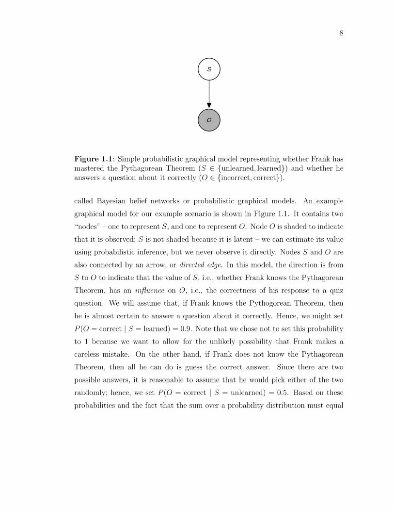
S
O
Figure 1.1: Simple probabilistic graphical model representing whether Frank hasmastered the Pythagorean Theorem (S ∈ {unlearned, learned}) and whether heanswers a question about it correctly (O ∈ {incorrect, correct}).
called Bayesian belief networks or probabilistic graphical models. An example
graphical model for our example scenario is shown in Figure 1.1. It contains two
“nodes” – one to represent S, and one to represent O. Node O is shaded to indicate
that it is observed; S is not shaded because it is latent – we can estimate its value
using probabilistic inference, but we never observe it directly. Nodes S and O are
also connected by an arrow, or directed edge. In this model, the direction is from
S to O to indicate that the value of S, i.e., whether Frank knows the Pythagorean
Theorem, has an influence on O, i.e., the correctness of his response to a quiz
question. We will assume that, if Frank knows the Pythogorean Theorem, then
he is almost certain to answer a question about it correctly. Hence, we might set
P (O = correct | S = learned) = 0.9. Note that we chose not to set this probability
to 1 because we want to allow for the unlikely possibility that Frank makes a
careless mistake. On the other hand, if Frank does not know the Pythagorean
Theorem, then all he can do is guess the correct answer. Since there are two
possible answers, it is reasonable to assume that he would pick either of the two
randomly; hence, we set P (O = correct | S = unlearned) = 0.5. Based on these
probabilities and the fact that the sum over a probability distribution must equal

9
1, we can also compute the conditional probability of an incorrect response:
P (O = incorrect | S = learned) = 1− P (O = correct | S = learned)
= 1− 0.9
= 0.1
P (O = incorrect | S = unlearned) = 1− P (O = correct | S = unlearned)
= 1− 0.5
= 0.5
Finally, let us suppose we have some prior belief about the value of S;
in particular, suppose that we have no idea whether Frank already knows the
Pythagorean Theorem. We might then set P (S = learned) = 0.5. If we had
evidence that Frank already knew this theorem, e.g., if we observed him reading
about it during class, then we might set this probability to a larger value.
Given that we have defined both a prior distribution over S as well as a
conditional probability distribution for O given S, we are now ready to conduct
Bayesian inference of the value of S. Let us suppose that Frank answers the math
problem incorrectly, i.e., O = incorrect. How much do we now believe that Frank
knows the Pythagorean Theorem, i.e., with what probability does S = learned
given that O = incorrect? To compute this probability P (S = correct | O =
incorrect) we will make use of Bayes’ rule, from which Bayesian statistics gets its
name:
P (S = learned | O = incorrect) =P (O = incorrect | S = learned)P (S = learned)
P (O = incorrect)(1.1)
Bayes rule tells us that the probability of S = learned given O = incorrect can be
computed (in part) by “flipping the conditionality around”, i.e., from the proba-
bility of O = incorrect given S = learned. This probability is already known to us
– in our example, we supposed it to be 0.1. The other term in the numerator on
the right hand side is P (S = learned) – our prior belief that S = learned – which
we supposed was 0.5.
To compute the denominator, we use the the law of total probability, which
tells us that P (O = incorrect) can be computed as the sum of probabilities of

10
giving an incorrect answer given either of the two knowledge states (“learned” or
“unlearned”), weighted by the probability of each knowledge state:
P (O = incorrect) = P (O = incorrect | S = unlearned)P (S = unlearned) +
P (O = incorrect | S = learned)P (S = learned)
= 0.5× 0.5 + 0.1× 0.5
= 0.3
Plugging this into Equation 1.1 we get:
P (S = learned | O = incorrect) =0.1× 0.5
0.3≈ 0.17
Hence, the posterior probability, or our posterior belief, that Frank knew the
Pythagorean Theorem, given his incorrect answer, is about 0.17. Compared to
our prior belief about Frank’s knowledge state, this is a rather large change.
It is instructive to also consider the case that Frank had given the correct
answer, and then to compute the posterior probability that he is in the “learned”
state:
P (S = learned | O = correct) =P (O = correct | S = learned)P (S = learned)
P (O = correct)
=0.9× 0.5
0.9× 0.5 + 0.5× 0.5
=0.45
0.45 + 0.25≈ 0.64
Notice the asymmetry here in how much we revise our belief that S = learned
when Frank gives a correct answer compared to when he gives an incorrect answer
– when Frank gives a correct answer, then we only slightly increase our belief. This
is because it is quite possible that he simply guessed correctly.
Finally, it is worth mentioning that Equation 1.1 is often written as a pro-
portionality, without the denominator, in order to avoid notational clutter:
P (S = learned | O = incorrect) ∝ P (O = incorrect | S = learned)P (S = learned)
(1.2)

11
1.4 Teaching as an Optimal Control Problem
Having given a whirlwind introduction to Bayesian inference, we now at-
tempt to motivate and illustrate the main concepts of the Partially Observable
Markov Decision Process (POMDP) using a hypothetical teaching scenario. The
example is highly simplistic and not intended to accurately model real students;
however, it is sufficiently rich to illustrate some of the fundamental challenges in
teaching and how algorithms for optimal control can be used to derive reasonable
teaching behavior.
Suppose that a teacher wishes to teach a student some skill. The student’s
knowledge of the skill is assumed to be binary, i.e, it is either “learned” or “un-
learned,” as in [14]. Hence, the state space S = {unlearned, learned}, and the
student’s state at time t is represented as St ∈ S. Although the teacher does not
observe the state St, it has a prior belief P (s1) over the student’s initial state S1.
Here, we assume that P (S1 = unlearned) = 1.
At each timestep, the teacher can perform one of three actions: it can
teach, meaning that the teacher attempts to transmit knowledge of the skill to the
student without eliciting any feedback from the learner; it can query the student’s
knowledge by asking him/her to demonstrate the skill; and the teacher can stop the
teaching session, after which no further teach or query actions can be performed.
Hence, the action space U = {teach, query, stop}, and the teacher’s action at time
t is represented by Ut ∈ U . When the teacher teaches, the student’s state may
transition with probability 0.2 from the unlearned to the learned state. If the skill
is already learned, then it will always stay learned, i.e., there is no “forgetting.”
When the teacher queries or stops, the student’s state does not change. The effects
of the teacher’s action on the student’s state constitute the transition dynamics
P (st+1 | st, ut) of the student; they are represented in Table 1.1.
During “query” actions, the student will attempt to demonstrate the skill
to the teacher, and the demonstration will either be correct or incorrect. Hence,
the observation space O = {incorrect, correct}. The student’s observation, i.e.,
his response to the teacher’s action at time t, is Ot. If the skill is learned, then
the student demonstrates the skill correctly with probability 1. If the skill is un-

12
Table 1.1: Transition dynamics for the simple teaching example of Section 1.4.
P (st+1 | st, Ut = teach)st+1
st unlearned learned
unlearned 0.8 0.2learned 0 1
P (st+1 | st, Ut ∈ {query, stop})st+1
st unlearned learned
unlearned 1 0learned 0 1
Table 1.2: Observation likelihoods for the simple teaching example of Section 1.4.
P (ot | st, Ut = query)ot
st incorrect correct
unlearned 0.9 0.1learned 0 1
P (ot | st, Ut ∈ {teach, stop})ot
st incorrect correct
unlearned 1 0learned 1 0
learned, then the demonstration is correct with probability 0.1 – the student must
essentially “guess” the right answer or “blindly” try to execute the skill correctly.
When the teacher executes the “teach” or “stop” actions, the student’s observation
is not meaningful; hence, we set the probability of a “correct” observation under
the “teach” and “stop” actions to be uninformative – the probability of each ob-
servation is independent of the student’s state. The probabilities P (ot | st, ut) of
which observation (“correct” or “incorrect”) the student emits as a function of the
teacher’s action and the student’s state constitute the observation likelihoods of
the teaching setting; they are shown in Table 1.2.
Given these three actions to choose from, how should the teacher act at each
timestep? How should the history of actions, along with the history of observations
received from the student, influence the teacher’s next action? Why should the
teacher bother to “query” the student at all, considering that such actions do not
directly influence the student’s state? These are the fundamental questions that
face all teachers, whether human or automatic, no matter what the exact teaching
setting is. Optimal control theory provides tools to tackle this problem. The next
step in solving our particular teaching problem using POMDPs is to define the
rewards and costs of teaching.

13
Table 1.3: Reward function r for the simple teaching example of Section 1.4.
ut st r(ut, st)teach unlearned −1teach learned −1query unlearned −0.5query learned −0.5stop unlearned 0stop learned 10
1.4.1 Immediate reward/costs
In optimal teaching problems, the teacher has a preference structure for
which actions it prefers to execute and in which states it prefers the student to
be. For instance, the teacher may prefer the student to be in the “learned” state
rather than in the “unlearned” state. This preference structure is expressed as an
immediate reward function r(ut, st), where ut ∈ U and st ∈ S. Costs of executing
certain actions can be formulated as negative-valued rewards. Note that these
rewards are not amounts of “money” that the teacher receives (or has to pay)
from someone while teaching – rewards are only used during planning to express
the teacher’s preferences for how the learning session should evolve.
In our example, the teaching and querying have associated costs; hence,
we set the corresponding immediate “rewards” to be −1 and −0.5, respectively,
regardless of the student’s state. If the teacher stops and the student’s knowledge
state was learned, then, in our example, there is a reward of 10. Together, the
immediate rewards are shown in Table 1.3. For an example from daily life, the
costs of teaching might consist of both the time that the teacher and student must
invest, as well as any monetary costs, e.g., salary, teaching supplies, etc. Note the
form that “querying” can play in modern education systems: standardized tests,
for example, may retrieve valuable information about students’ knowledge, but
they also interrupt normal school instruction and hence incur a cost.
The goal of the teacher in optimal teaching scenarios is to execute actions
so as to maximize the expected long-term reward (or minimize the expected long-
term cost). The teacher chooses its actions based on a control policy. It turns
14
out that this control policy can be formulated as a function of the teacher’s belief
about the student’s state; in fact, the belief is a sufficient statistic of the teaching
history in order to maximize the expected long-term reward. We define belief and
the belief update process below.
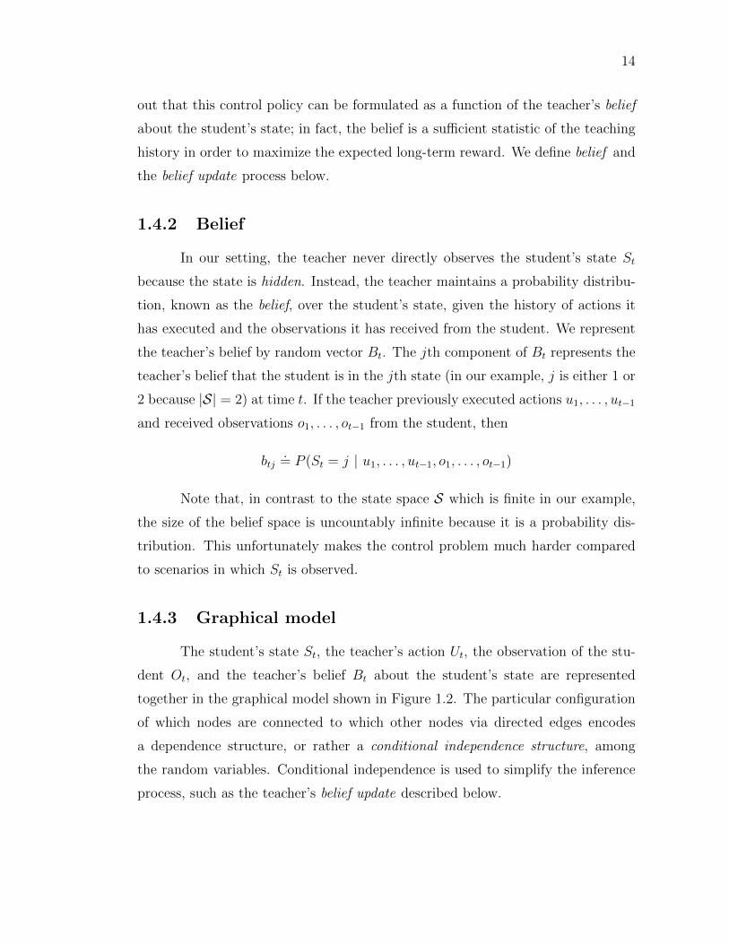
1.4.2 Belief
In our setting, the teacher never directly observes the student’s state St
because the state is hidden. Instead, the teacher maintains a probability distribu-
tion, known as the belief, over the student’s state, given the history of actions it
has executed and the observations it has received from the student. We represent
the teacher’s belief by random vector Bt. The jth component of Bt represents the
teacher’s belief that the student is in the jth state (in our example, j is either 1 or
2 because |S| = 2) at time t. If the teacher previously executed actions u1, . . . , ut−1
and received observations o1, . . . , ot−1 from the student, then
btj.= P (St = j | u1, . . . , ut−1, o1, . . . , ot−1)
Note that, in contrast to the state space S which is finite in our example,
the size of the belief space is uncountably infinite because it is a probability dis-
tribution. This unfortunately makes the control problem much harder compared
to scenarios in which St is observed.
1.4.3 Graphical model
The student’s state St, the teacher’s action Ut, the observation of the stu-
dent Ot, and the teacher’s belief Bt about the student’s state are represented
together in the graphical model shown in Figure 1.2. The particular configuration
of which nodes are connected to which other nodes via directed edges encodes
a dependence structure, or rather a conditional independence structure, among
the random variables. Conditional independence is used to simplify the inference
process, such as the teacher’s belief update described below.
15
St St+1
Bt Bt+1
π
Ut
Ot
... ...
Belief
State
Action
Observation
Policy
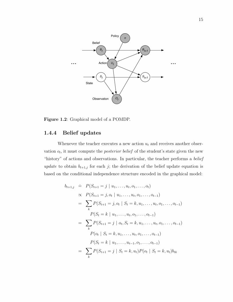
Figure 1.2: Graphical model of a POMDP.
1.4.4 Belief updates
Whenever the teacher executes a new action ut and receives another obser-
vation ot, it must compute the posterior belief of the student’s state given the new
“history” of actions and observations. In particular, the teacher performs a belief
update to obtain bt+1,j for each j; the derivation of the belief update equation is
based on the conditional independence structure encoded in the graphical model:
bt+1,j.= P (St+1 = j | u1, . . . , ut, o1, . . . , ot)
∝ P (St+1 = j, ot | u1, . . . , ut, o1, . . . , ot−1)
=∑k
P (St+1 = j, ot | St = k, u1, . . . , ut, o1, . . . , ot−1)
P (St = k | u1, . . . , ut, o1, . . . , ot−1)
=∑k
P (St+1 = j | ot, St = k, u1, . . . , ut, o1, . . . , ot−1)
P (ot | St = k, u1, . . . , ut, o1, . . . , ot−1)
P (St = k | u1, . . . , ut−1, o1, . . . , ot−1)
=∑k
P (St+1 = j | St = k, ut)P (ot | St = k, ut)btk

16
The first term in the summation of the last line comes from the transition dy-
namics ; the second term is from the observation likelihood ; and the last term is
the teacher’s prior belief of the student’s state at time t. This equation allows
the teacher to efficiently compute the belief update by summing over its prior be-
liefs for each possible state and weighting them by the product of the transition
probability and observation likelihood.
1.4.5 Control policy
At each timestep t, the teacher must select an action Ut to execute. The
teacher chooses this action according to a control policy π. A deterministic policy
maps from bt into an action ut ∈ U ; a stochastic policy maps from bt into a
probability distribution over U . In the case of a stochastic policy, to choose the next
action, the teacher would first compute π(bt), and then sample an action from the
resultant probability distribution. Different policies tend to choose certain actions
more often than others, and they may cause the student to enter certain states
more frequently. Since the teacher associates rewards with these state+action
combinations, some policies may be better than others in terms of the teacher’s
preferences; this is quantified by the value function V (π) which computes the
expected sum of discounted rewards over the time horizon τ :
V (π).= E
[τ∑t=1
γtr(St, Ut) | π, P (s1)
]The time horizon τ specifies the length of the teaching session, and the discount
factor γ ∈ [0, 1] specifies how much rewards in the near future are to be weighted
compared to rewards in the distant future. If γ is small, then rewards in the distant
future have little effect on the value of a particular policy. Choosing τ =∞, which
is admissible as long as γ < 1, is a mathematical convenience that allows for the
formulation of a stationary policy that does not change as a function of time.
Given the formula for V above, an optimal (stationary) policy is a function π∗
that maximizes V :
π∗.= arg max
πV (π)
In our example, we choose γ = 0.99 and τ =∞.

17
1.4.6 Partially Observable Markov Decision Processes
We have now defined all the variables that constitute a Partially Observable
Markov Decision Process (POMDP). Formally, a POMDP is defined by a tuple
(S,U ,O, P (st+1 | st, ut), P (ot | st, ut), r(u, s), τ, γ, P (s1))
whose components are the state space, action space, observation space, transition
dynamics, observation likelihood, reward function, time horizon, discount factor,
and prior belief of the student’s state, respectively.
The challenge when working with POMDPs to solve teaching problems
is to compute the policy π according to which the teacher will act. In some
very restricted teaching scenarios, the optimal policy π∗ can be found analytically
(e.g., [81]). Otherwise, numerical methods must be used. The method of value
iteration [17], which is based on dynamic programming, can be used to estimate
the optimal policy of a POMDP with arbitrary precision, but the computational
costs are formidable: for a time horizon τ , the worst-case time cost is O(22τ ). The
reason for the enormous time complexity for exact solutions is that the state St is
hidden, and hence all teaching decisions must be made in terms of a real-valued
belief Bt instead of the (typically) discrete-valued St. Due to the computational
costs, a variety of approximation methods are typically used to solve POMDPs for
real-world control applications. Approximate methods based on belief compression
(e.g., [74]) seek to reduce the size of the state space to speed up computation.
Point-based value function approximation methods (e.g., [83]) give up on trying to
find a policy that works well for all beliefs bt and instead focus on the most likely
beliefs that the agent (teacher) would encounter. Finally, policy gradient methods
(e.g., [98, 15]) formulate the policy π using a parameter vector and use gradient
descent to maximize V with respect to the policy’s parameters. In Chapter 5 of
this thesis, we use a policy gradient approach to optimize our word teacher.
For now, however, let us return to the simple teaching example we sketched
above, and let us examine how the optimal policy behaves. We used the ZMDP
software [82], which internally uses point-based value iteration, to compute the
optimal policy, shown in Figure 1.3. The horizontal axis of the figure shows the

18
0 0.2 0.4 0.6 0.8 13
4
5
6
7
8
9
10
p(Learned)
Value
Value versus belief
Teach Query Stop
Figure 1.3: Optimal policy for the simple teaching example in Section 1.4.
teacher’s belief bt that the student is in the “learned” state, and the vertical axis
shows the value, i.e., the expected sum of discounted future rewards given the
optimal policy π∗ and the teacher’s current belief, associated with b. In addition,
the vertical bars in the graph separate the “regions” of the belief space within which
a certain action is optimal. According to the computed policy, the “teach” action
is optimal when the teacher has a small belief that the student is in the “learned”
state, and the “stop” action is optimal when the teacher has a large belief that the
student has learned the skill. Interestingly, it turns out that, when the teacher’s
belief is uncertain, i.e., between about 0.3 and 0.82, then the optimal action is to
“query” the student. Note that querying does not immediately help the student
to learn the skill; rather, it helps the teacher to become more certain about the
student’s state and thereby to make more intelligent actions in the future. In the
framework of stochastic optimal control, such “information foraging” actions can
emerge naturally as the optimal action because they implicitly help the teacher to
minimize the expected long-term cost.
Let us now recapitulate what it means to pose “teaching” as an optimal
control problem using the language of POMDPs: the teacher executes actions so as

19
to alter the student’s state in ways that the teacher finds desirable according to its
reward function. However, the teacher cannot directly observe the student’s state
because it is “hidden” inside the student’s mind; instead, it can only maintain and
update a belief about the student’s state given the history of actions and observa-
tions it has received from the student during the learning session. The teacher’s
action at each timestep is chosen acording to a control policy which maps the
teacher’s current belief into an action (or a probability distribution over actions).
An optimal control policy chooses actions, based on the teacher’s current belief, so
as to maximize the expected long-term reward, or equivalently, to minimize the
expected long-term cost, of teaching.
In practice, successful application of control theoretic methods to optimal
teaching problems requires effective use of approximate methods to finding good
policies. Although the simple example we presented in this section modeled the
state as a binary variable, in Chapter 5 of this dissertation we consider a much more
complex learning model: the student’s state is a set of probability distributions over
the meanings of a set of words, and the teacher’s belief is therefore a probability
distribution over a set of probability distributions. Despite the enormity of the
belief space, a good policy was still found using a policy gradient optimization
approach.
1.5 Affect-sensitive teaching
So far in our modeling of teaching as an optimal control problem we have
only considered the “cognitive” elements of a student’s state, e.g., whether the
student knows some skill, or whether his answer to a question is right or wrong.
Let us now come to the crux of the dissertation and consider the importance of the
non-cognitive, or what we call the affective, components of a student’s state, e.g.,
how the student feels, whether the student is attentive, whether he/she is trying
to learn, etc. In addition, let us also examine the affective components of the
observations the teacher receives of the student – does the student appear attentive
based on visual and auditory information we receive? Does the student look like

20
SKt SKt+1
Bt Bt+1
π
Ut
OKt
... ...
Belief
State
Action
Observation
SAt SAt+1
OAt
Policy
Figure 1.4: POMDP to model affect-sensitive teaching. SKt is the student’s“knowledge state”, SAt is the student’s “affective state”.
he’s trying to succeed? To illustrate this shift from a purely “cognitive” view of
teaching to an “affect-sensitive” perspective, we have created a revised graphical
model to include both affective and cognitive state and both affective and cognitive
observations, shown in Figure 1.4. In the figure, the student’s state is split into
the knowledge state SKt and the affective state SAt . Similarly, the observation Ot
is split into the knowledge observation OKt and the affective observation OA
t .
1.5.1 Affective and cognitive transition dynamics
Given the new “affect-sensitive” POMDP, we can examine more concretely
how modeling of affect – whether in the state or the observation – could impact
both learning and teaching. Let us first consider the influence of the knowledge and
affective state components both on themselves and each other. These influences
are shown in Figure 1.5 (a). Arrow 1, from SKt to SKt+1 represents the fact that
the student’s knowledge at time t influences her knowledge at time t + 1. This is
natural – if a student has mastered differential calculus at time t, then it is very
unlikely that she would suddenly lack the knowledge to solve a linear equation at

21
time t+ 1. Similarly, arrow 4 represents the fact that a student’s emotional state
at t will likely have some effect on his emotional state at t+ 1 – emotions, though
possibly erratic, will likely show some temporal consistency.
More interesting and subtle are the other two arrows. Arrow 2 represents
the influence of a student’s knowledge on her affect. As an arbitrary example, it is
possible that, if a student cannot manage to learn a certain topic for a long time,
i.e., her knowledge state stagnates, then this lack of progress could impact the
student’s affective state, e.g., cause her to become frustrated. Arrow 3 represents
the opposite effect – if a student is frustrated, then she may have difficulty learning
the curriculum, causing her knowledge state to stagnate.
Note that, as a teacher, we may associate value with both the knowledge
and affective components of the student’s state. We may care that the student be
in a positive affective state so that she can learn better (i.e., because we value SKt ),
but we may also wish for the student to be in a positive affective state just for the
sake of the student’s happiness (i.e., because we value SAt ). Both kinds of value
that we associate with the student’s state can influence our teaching decisions.
1.5.2 Affective and cognitive observation likelihood
Next, Figure 1.5 (c) portrays how the state components are reflected in the
observations. Arrow 1 is natural and represents how the student’s knowledge influ-
ences his test answers, factual responses to the teacher’s questions, etc. Similarly,
arrow 3 represents how the student’s affective state is reflected in affective obser-
vations made of the student – for instance, though a student may try to mask his
emotional state, it is likely that an expert teacher (or a highly accurate automatic
emotion classifier) can at least partly perceive that emotion. Arrow 2 is more sub-
tle and represents how the student’s affective state can impact how he performs –
if he is not trying, then his test scores may be low, regardless of what he knows or
how skilled he is. If the teacher, whether human or computer, attributes poor test
performance to the wrong cause, then this can lead to bad teaching.

22
1.5.3 Belief updates using affective observations
Finally, Figure 1.5 (b) represents how the observations of the student – both
knowledge and affective – are used to update the teacher’s belief about the stu-
dent’s state. Node OAt is half-shaded to indicate that, depending on the particular
learning setting, it may or may not be observed by the teacher. In Chapter 2 of this
dissertation, we examine the impact on teaching effectiveness of the teacher having
access to the affective observations, specifically being able to view the student’s
face while teaching.
1.5.4 Designing affect-sensitive teachers
Good human teachers are adept at knowing which aspects of a student’s
cognitive and affective state and which kinds of observations he/she receives from
the student are important and which can be ignored. Similarly good judgment
is required when designing effective automated teachers. In particular, as the de-
signer of an ITS, we need to decide which nodes and which directed edges of the
affect-sensitive POMDP in Figures 1.4 and 1.5 we will include in our teaching
model. For instance, perhaps in a given learning domain we, as the teacher, can
completely ignore the student’s “affective observations” because all of the useful
information is already contained in the student’s test performance. In this case,
making the teacher “affect-sensitive” might well be a waste of time. The impor-
tance to teaching effectiveness of the teacher being able to see some of the student’s
affective observations is a question we tackle in Chapter 2. If, on the other hand,
we decide that using affective observations is important, then we need a mecha-
nism of regressing from those observations to the student’s state. In Chapters 3
and 4 we thus develop automatic classifiers of student “engagement” and student
perception of curriculum difficulty that map from the pixels of the student’s face
to these affective states. Finally, and most crucially, creating automated teachers
requires that we devise a control policy for how the teacher should act. This con-
trol policy should deliver good learning gains and should be tractably computable
given a reasonable model of the learner. In Chapter 5, we propose an automated
procedure for computing a control policy for the particular domain of language

23
SKt SKt+1State
SAt SAt+1
12
34
Bt+1
OKt
OAt
Observation
SKt
OKt
State
Observation
SAt
OAt
1
23
πPolicy
Belief
Chapter 2
Chapters 3 & 4
Chapter 5
a bc d
Figure 1.5: Dissertation roadmap.
learning.
1.6 Dissertation outline and contributions
The rest of this dissertation is structured as follows: In Chapter 2 we pro-
pose and demonstrate an experimental protocol for measuring the importance to
teaching of having access to the “affective observations” of the student. This is
a useful procedure to execute prior to investing the effort to develop an affect-
sensitive automated teacher for a given learning domain – if affective sensors make
no difference, then using them is probably a waste of time. We apply this experi-
mental framework to cognitive skills training, which is a training regimen designed
to boost students’ performance in academic subjects by first improving basic mem-
ory, attention, and logical reasoning abilities. This project emerged out of a col-
laboration with the Serpell lab at Virginia State University. Zewe Serpell visited
our lab as a visiting scholar during Summer 2010, and I visited her lab in Virginia
24
twice during the ensuing two years.
Chapters 3 and 4 consider the problem of recognizing important aspects
of students’ affective state from affective sensor measurements. While the com-
puter vision and automatic face analysis communities have studied extensively
the problems of basic emotion (e.g., [51, 103, 55]) and facial action [32] (e.g.,
[50, 102, 58, 9, 88]) recognition, much less work has been done recognizing more
nebulously defined affective states related to learning. It is thus unclear how well
existing methods for both labeling video and image data, and for estimating these
labels automatically, would work in practice in automated teaching settings. In
Chapter 3 we attempt to detect students’ degree of “engagement” with their learn-
ing task; here, we make use of the video data we collected as part of the Cognitive
Games study from Chapter 2. As the “ground truth” for students’ engagement
scores, we use the perceptual judgments of human observers who viewed either
video clips or images of students interacting with the game software. This may
not be a perfect label of student’s engagement state, but we would already be
very happy if a machine could predict what human observers would say about
a student’s level of engagement. In contrast, in Chapter 4, we ask the students
themselves how hard or easy they perceive the curriculum of a lecture video to
be at each moment in time, and then attempt to estimate these perceived diffi-
culty scores automatically. In both these chapters we make use of the Computer
Expression Recognition Toolbox (CERT), which is a tool for automated real-time
face processing developed at our laboratory (and to which this dissertation author
contributed several components including the smile detector [95] and head pose
estimator [96]), and attempt to regress from CERT’s output channels to more
subjective categories such as “engagement” and “perceived difficulty”.
Finally, in Chapter 5, we present and evaluate a prototype automatic teach-
ing system whose controller was computed so as to minimize the expected time
needed by the student to learn the material and pass the test. The teaching prob-
lem is modeled as a POMDP, and the student is modeled as a Bayesian learner
who conducts probabilistic inference in the same manner as described in Section
1.3; hence, our system is an example of applying model-based control techniques

25
to develop an automated teacher. The target learning domain is foreign langugae
learning by image association. For instance, to teach the meaning of the German
word trinken, the program might show an image of a girl drinking a cup of milk,
followed by an image showing a man drinking tea. From these word+image pairs,
a rational student could reasonably infer that trinken probably means “drink”.
This is the same teaching approach used Rosetta Stone language software [73] and
the Web-based DuoLingo learning system [30]. While an automated, optimized
teacher for this domain is useful in its own right, the greater goal of this chapter is
to propose and demonstrate methods for constructing automated teachers using a
principled decision framework such as POMDPs. After showing that the learned
teaching engine performs favorably compared to two baseline controllers, we de-
scribe a plausible architecture for how it might be extended to incorporate affective
observations and demonstrate in simulation the potential benefits of doing so.

Chapter 2
Measuring the Benefit of
Affective Sensors
Abstract : While affect-sensitive automated teaching systems are becoming
an active topic in the ITS community, there is yet no consensus whether respon-
siveness to students’ affect will result in more effective teaching systems. Even
if the benefits of affect recognition were well established, there is yet no obvious
path for creating an affect-sensitive automated tutor. In this chapter we present
an experimental protocol for measuring the effect on teaching of being able to see
the student’s face during teaching. The learning setting we focus on is cognitive
skills training. In addition, while conducting the experiment, we simultaneously
collect training data with ecological validity that could later be used to develop
an automated teacher on cognitive skills. Experimental results suggest that affect-
sensitivity in the cognitive games setting is associated with higher learning gains.
Behavioral analysis using automatic facial expression coding of recorded videos
also suggests that smile may reveal embarrassment rather than achievement in
learning scenarios.
2.1 Introduction
Until recently, ITS typically employed only a relatively impoverished set of
sensors consisting of a keyboard and mouse, which amounts to only a few bits per
26

27
second that they process from the student. While various researchers in the field
of ITS have been migrating towards modeling affect in their instructional systems
[99, 26, 94], there is, surprisingly, no firm consensus yet on whether affect sensitiv-
ity actually makes better automated teachers: In his keynote address [89] to the
ITS’2008 conference in Montreal, Kurt VanLehn, a prominent ITS researcher who
pioneered the Andes Physics Tutor [90], asserted that affective sensors such as au-
tomatic facial expression recognition systems were not useful in ITS, and efforts to
utilize them for automated teaching were misguided. Indeed, it is conceivable that
the explicit feedback given by the student to the teacher in the form of keystrokes,
mouse clicks, and screen touches might constitute all that is needed for the teacher
to teach well. On the other hand, we posit two reasons why modeling of affect
may be important: (1) State preference: Certain affective states in the student
may be more desirable than others. For example, a teacher might wish to avoid a
situation in which the student becomes extremely upset while attempting to solve
a problem. (2) State disambiguation: Consider a student who has been asked a
question and who has not responded for several seconds. Is the student confused?
Is he/she still thinking of the answer and just about to respond? Or has the stu-
dent disengaged completely and perhaps even left the room? Without some form
of affective sensors, these very different states may not be easily distinguished.
In this chapter we tackle two problems: (1) For one particular domain
of learning – cognitive skill training (described in Section 2.3) – we investigate
whether affective state information is useful for human teachers to teach effectively.
We analyze the utility of affective state in terms of learning gains as assessed by a
pre-test and post-test on a spatial reasoning task. We use a Wizard-of-Oz (WOZ)
paradigm to simulate the environment a student would face when interacting with
an automated system. While conducting this experiment, we also (2) Collect data
that could be used to train an automated cognitive skills teacher. These data
consist of timestamped records of the student’s actions (e.g., move cards on the
screen), the teacher’s commands (e.g., change task difficulty), and the student’s
face video. The ultimate goal of our research is to identify learning domains in
which affect sensitivity is useful to human tutors, and to develop automated sys-

28
tems that utilize affective information the way human tutors do.
2.2 Related work
Although a number of affect-aware ITS have emerged in recent years, such
as affect-sensitive versions of AutoTutor [26] and Wayang Outpost [99], it is still
unclear how beneficial the affect sensitivity in these systems actually is. Some
research has been conducted on the impact of the use of pedagogical agents on
student’s engagement and interest level [99], but studies on the impact of actual
learning gains are scarce. The only study to our knowledge that specifically ad-
dresses this point is by Aist, et. al [1]: They augmented an automated Reading Tu-
tor, designed to boost reading and speech skills by asking students to read various
vocabulary words out loud, with emotional scaffolding using a WOZ framework.
In their experiment, a human teacher (in a separate room) watching the student
interact with the tutor could provide supplementary motivational audio prompts
to the student, e.g., “You’re doing fine.” Compared with students in a control
condition who received no emotional scaffolding, students in the affect-enhanced
condition chose to persist in the learning task for a longer time. However, no sta-
tistically significant increase in learning gains was found. In their study, the only
action the human teachers could execute was to issue a prompt – teachers could
not, for instance, also change the task difficulty. Moreover, the study did not assess
whether the tutors could have been as effective if they did not have access to the
video of the student, i.e., if their prompts had been based solely on the student’s
accuracy on the task.
2.3 Cognitive skills training
In recent years there has emerged growing interest in “cognitive training”
programs that are designed to hone basic skills such as working memory, attention,
auditory processing, and logical reasoning. The motivation behind cognitive skills
training is that if basic cognitive skills can be improved, performance in academic

29
subjects such as mathematics and reading may also increase. In recent years cog-
nitive training has been shown to correlate both with increased cognitive skills
themselves [60] as well as increased performance in mathematics in minority stu-
dents [42]. Certain cognitive training regimes have also been shown to boost fluid
intelligence (Gf), with larger doses of training associated with larger increases in
Gf [45].
In some cognitive skill training programs such as Learning Rx [54], cognitive
training sessions are conducted 1-on-1 by a human trainer. Since employing a
skilled human trainer for every pupil is expensive, it would be useful to automate
the cognitive training process, while maintaining the benefits of having a human
teacher.
2.3.1 Human training versus computer training
Learning Rx prescribes a dose of both 1-on-1 human-facilitated training,
along with “homework” consisting of computer-based training of the same skills
using the same games. In a study comparing the effectiveness of human-based
versus computer-based learning with Learning Rx cognitive skill-building games,
Hill, et. al found that human-based 1-on-1 training was more effective in terms of
learning gains both on the cognitive skills tasks themselves as well as in associated
mathematics performance [42]. When trying to develop an automated teaching
system of cognitive skills, it is important to understand the causes of this result.
We suggest three different hypotheses:
1. Skill level hypothesis: Human teachers are very adept at adapting their
teaching to the the student’s apparent skill level and explicit game actions.
2. Affect-sensitivity hypothesis: Human teachers can adapt to the affective
state of the student and thereby teach more effectively.
3. Mere presence hypothesis: The mere presence of a human observer can
positively influence the student’s performance [41].
Suppose that, in a given learning domain, the reason why human tutors are more
effective is because of the skill level hypothesis. Then the benefit of making an

30
automated teaching system affect sensitive may be minimal and not worthwhile.
Similarly, if the mere presence of a human or perhaps a human teacher’s ability
to converse freely with the student using perfect speech recognition is the deciding
factor in effectiveness, then there is little hope that an automated system can match
a human. If, however, affect sensitivity is important for the human teacher, then
it may also prove useful for automated systems. In the experiment we describe in
the next section, we evaluate the three hypotheses above.
2.4 Experiment
We conducted an experiment to assess the importance of affect in cognitive
skills training by an automated teacher. Since we have not yet built such a system,
we simulate it using a WOZ paradigm. In WOZ experiments, a human operates
behind a “curtain” (a wall, in our case), unbeknownst to the student, and controls
the teaching software. For our experiment we developed a battery of three cognitive
games that we developed for the Apple iPad:
• Set: Similar to the classic card game, Set consists of cards that contain
shapes with multiple attributes including size, shape, color, and (for higher-
difficulty levels) orientation. The goal is to make as many valid “sets” of 3
cards each during the time allotted. A set is valid if and only if, for each
dimension, the values of the three cards are either all the same or all different.
• Remember: A series of randomly generated patterns appear for a brief
moment (the duration depends on the current difficulty level) on the screen.
If the current pattern is the same as the previous pattern, then the student
presses the left button on the screen. If the pattern is different, he/she
presses the right button. At each time step the student must both act (press
a button) and remember the current card.
• Sum: Similar to Remember, a series of small integers is presented to the
user at a variable rate dependent on the current difficulty level. If the sum

31
Figure 2.1: A screenshot of the “Set” game implemented on the Apple iPad forthe cognitive skill learning experiment.
of the current and previous numbers is even, then the user presses the left
button; if it is odd, he/she presses the right button.
During piloting, students typically found the Set game the most challenging, and
the other two tasks were perceived as more recreational and diverting. Hence,
we used Set as the primary task that teachers should focus on. The other two
tasks were provided as options to the teachers with which to give “breaks” to the
students. However these breaks were to be taken only to the extent that they
would help with the long term performance on Set. Before each training session,
each student performed a 2-minute pre-test on Set, and after the training session
(30 minutes) each student performed a 2-minute post-test on the same task. The
performance metric during tests was the number of valid sets the student could
make in the time allotted. A screenshot of Set (recorded on the iPad simulator) is
shown in Figure 2.1. Students control by the game by touching an iPad-1. Student
actions consist of dragging cards in the Set task, and pressing a Left or Right button
during the Remember and Sum tasks. The students’ game inputs, along with
videos of their face and upper body, were timestamped and recorded. In addition,
we also recorded the teacher’s actions, which consisted of increasing/decreasing
task difficulty, switching tasks, giving a hint, and providing motivation in the form

32
of pre-recorded audio prompts. The teachers were instructed to execute whatever
commands they deemed necessary in order to maximize the student’s learning
gains on Set. These data was collected with an eye towards analyzing the teaching
policies used by teachers and porting them into an automated teacher (see Section
2.6).
2.4.1 Conditions
We compared learning gains on Set across three experimental conditions:
1. 1-on-1: The student works 1-on-1 with a human trainer who sits beside the
student and makes all teaching decisions. The student is free to converse
with the teacher. All of the student’s and teacher’s actions on the iPad, as
well as a video of the student, are recorded automatically and synchronously.
2. WOZ (full): The student works by him/herself on the iPad. The student is
told that the iPad-based game software is controlled by an automatic teacher.
In reality, it is controlled by a human trainer in another room who sees both
the student’s actions on the iPad as well as the student’s face and upper
body behavior over a videoconference. The student does not see or hear the
teacher. The teacher’s actions, student’s actions, and student’s video are all
recorded automatically and synchronously.
3. WOZ (blind): This condition is identical to the WOZ (full) except that
the teacher cannot see or hear the student – the video camera records the
student’s behavior but does not transmit it to the teacher. In other words, the
teacher is forced to teach without seeing the affective information provided
by the student’s face, gestures, and body posture.
Of all the students we interviewed afterwards who had participated in a WOZ
condition, none suspected that the “automated teacher” was actually human.
The three conditions were designed to help distinguish which of the three
hypotheses given in Section 2.3.1 is most valid. Consider the following possi-
ble outcomes, where performance is measured in learning gains (PostTest minus
PreTest):

33
TeacherStudent
TeacherStudent
Record video only.
Record video.Send video to teacher.
Remote control of iPad teaching software.
Wall
Record video only.
1-on-1
Wizard-of-Oz (full)
Wizard-of-Oz (blind)
Live video of student.
TeacherStudent
Remote control of iPad teaching software.
Wall(No live video of student.)
Figure 2.2: Three experimental conditions. Top: Human teacher sits with thestudent in a 1-on-1 training setting. Middle: An “automated” teacher is simu-lated using a Wizard-of-Oz (WOZ) technique. The iPad-based game software iscontrolled by a human teacher behind a wall. The teacher can see live video ofthe student. Bottom: Same as middle condition, except the teacher cannot seethe live video of the student – the teacher sees only the student’s explicit gameactions.
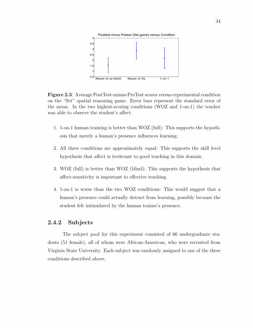
34
Wizard−of−oz (blind) Wizard−of−Oz 1−on−10.5
1
1.5
2
2.5
3
3.5
4Posttest minus Pretest (Set game) versus Condition
Figure 2.3: Average PostTest-minus-PreTest scores versus experimental conditionon the “Set” spatial reasoning game. Error bars represent the standard error ofthe mean. In the two highest-scoring conditions (WOZ and 1-on-1) the teacherwas able to observe the student’s affect.
1. 1-on-1 human training is better than WOZ (full): This supports the hypoth-
esis that merely a human’s presence influences learning.
2. All three conditions are approximately equal: This supports the skill level
hypothesis that affect is irrelevant to good teaching in this domain.
3. WOZ (full) is better than WOZ (blind): This supports the hypothesis that
affect-sensitivity is important to effective teaching.
4. 1-on-1 is worse than the two WOZ conditions: This would suggest that a
human’s presence could actually detract from learning, possibly because the
student felt intimidated by the human trainer’s presence.
2.4.2 Subjects
The subject pool for this experiment consisted of 66 undergraduate stu-
dents (51 female), all of whom were African-American, who were recruited from
Virginia State University. Each subject was randomly assigned to one of the three
conditions described above.

35
2.5 Experimental results
2.5.1 Learning conditions
Performance was measured as the average PostTest minus PreTest score
across each condition; results are shown in Figure 2.3. Although the differences
(assessed by 1-way ANOVA) were not statistically significant, the two higher-
performance conditions were WOZ (full) and 1-on-1. These were the two conditions
in which the student’s affect was visible to the teacher, thus suggesting that affect
sensitivity may indeed be important for this learning domain. Interestingly, the
WOZ (full) was also higher than 1-on-1 – it is possible that the human teacher’s
presence was intimidating for some students and thus led to smaller learning gains.
2.5.2 Facial expression analysis
In addition to assessing differences in learning gains, we also examined
how learning performance relates to students’ facial expressions. One particular
question of note is the role of smile in learning: Does occurrence of smile per-
haps indicate mastery? To investigate this question we performed automatic smile
detection across the videos collected of the students during the game play. We
employed the Computer Expression Recognition Toolbox (CERT) [57], which is a
tool for fully automatic real-time facial expression analysis from video.
To our surprise, the correlation between the average smile intensity (as es-
timated by CERT) over each video with PostTest-minus-PreTest performance was
−0.34 (p < 0.05). In other words, students who learned more tended to smile
less. This suggests that the smiles that do occur may be due more to embarrass-
ment than to a sense of achievement. This also dovetails with findings by Hoque
and Picard [44], who found that smiles frequently occur during natural episodes
of frustration. Broken down by gender, the correlations were r = −0.24 for male
(p > 0.05, N = 15), and r = −0.35 for female (p < 0.05, N = 51), suggesting that
the effect may be more pronounced for females. We caution, however, that the
reliability of CERT’s smile detector on the cognitive training data has yet to be
thoroughly validated against manual expression codes. Accuracy of contemporary

36
Figure 2.4: Left: A student who smiles as a result of receiving and acting upon a“giveaway” hint after having not scored any points for approximately 20 seconds.Right: A student who smiles after making a mistake, which resulted in a “buzzer”sound.
Figure 2.5: A student who is in the midst of scoring multiple points.
face detection and smile detection systems on dark-skinned people in particular is
known to be less reliable than for other ethnicities [95].
Examples of smiles that occurred during the experiment are shown in Figure
2.4. In Figure 2.4 (right), the subject had just made a mistake (formed an invalid
set from 3 cards) which resulted in the game making a “buzzer” sound. Similarly,
in Figure 2.4 (left), the teacher had just given a “give-away” hint consisting of all 3
cards necessary to form a valid set. The student “took” the hint (made the hinted
set) and then produced the expression shown, which suggests that she may have
been embarrassed at needing the assistance. In contrast, the subject in Figure
2.5 was in the midst of scoring multiple points in rapid succession. Her facial
expression during this time period shows relatively little variability in general, and
no smile in particular.

37
Time
Student's actions
Student's video
Give a hintIncrease task
difficultyTeacher's actions
Figure 2.6: An example of the “traces” collected of the student’s actions, thestudent’s video, and the teacher’s actions, all recorded in a synchronized manner.
2.6 Towards an automated affect-sensitive teach-
ing system
The pilot experiment described above was conceived both to evaluate the
hypotheses discussed in Section 2.3, and also to simultaneously collect training
data that can be used to create an automated cognitive skills trainer. Recall that,
in the WOZ (full) condition, the student interacts with an apparently “automated”
iPad-based teacher, and that in this experimental condition no human was present.
This interaction setting closely resembles the setting in which the student interacts
with a truly automated trainer. Were training data collected from a 1-on-1 setting
in which the student interacted with another human, the elicited affective states
and behavior might be very different, and the collected training data might lead
the automated system astray.
Given the “traces” of interactions between students and teachers recorded
during the experiment (see Figure 2.6), there are several possible strategies for how
to develop an affect-sensitive tutor, including rule-based expert systems, stochastic
optimal control [6, 19], machine learning, or perhaps some combination of the three.
In Woolf, et. al [99], for example, the authors combine manually coded rules with
machine learning.
In our project we are pursuing a machine learning approach toward devel-

38
oping an affect-sensitive tutor:
1. Ask expert human teachers to label the key affective states of the student
based both on the student’s actions and his/her video.
2. Perform automatic facial expression recognition on the student’s video, in
order to convert the raw video into a form more amenable to automated
teaching. Classifiers such as CERT [57] output the estimated intensity of a
set of facial muscle movements.
3. Train affective state classifiers that map from the outputs of the facial
expression classifier to the higher-level states labeled in the first step.
4. Use supervised learning to compute a policy, i.e., a map from a history of
estimated affective states extracted from the live video, the student’s actions,
and the teacher’s previous actions, into the teacher’s next action. The data
necessary for training are available in the recorded traces.
2.7 Summary and further research
We have presented results from a pilot study assessing the importance of
affect in automated teaching of cognitive skills. Results suggest that availability of
affective state information may allow the teacher to achieve higher learning gains
in the student. In addition, we have found evidence that smile during learning
may indicate more embarrassment than achievement. Finally, we have proposed a
methodology and software framework for collecting training data from the afore-
mentioned experiment that can be used to train a fully automated, affect-sensitive
tutoring agent. In future research we will extend the cognitive training experiment
from 1 day to 6 days in an effort to elicit states with more variety, e.g., with more
student fatigue.

39
2.8 Acknowledgement
Support for this work was provided by NSF grants SBE-0542013 and CNS-
0454233, and an NSF Leadership Development Institute Fellowship from HBCU-
UP to Dr. Serpell. Any opinions, findings, and conclusions or recommendations
expressed in this material are those of the author(s) and do not necessarily reflect
the views of the National Science Foundation.
Chapter 2, in full, is a reprint of the material as it appears in IEEE Com-
puter Society Conference on Computer Vision and Pattern Recognition Workshops
(CVPRW), 2011. Jacob Whitehill, Zewelanji Serpell, Aysha Foster, Yi-Ching Lin,
Brittney Pearson, Marian Bartlett, and Javier Movellan. The dissertation author
was the primary investigator and author of this paper.
Chapter 3
Automatic Recognition of
Student Engagement
Abstract : In contrast to the more thoroughly studied problems of basic
emotion (e.g., happy, sad) and facial action unit recognition [32], relatively little
research has addressed the problem of automatically recognizing educationally rel-
evant affective states such as frustration, boredom, fatigue, and engagement. In
this chapter, we examine a dataset of 34 undergraduate subjects undergoing cogni-
tive skills training on an Apple iPad and assess how well the degree of a student’s
engagement, as perceived by external observers, can be estimated automatically
using modern computer vision and machine learning methods. Results indicate
that, for subject-independent binary classification (e.g., Engagement = 4 versus
Engagement 6= 4), machine classifiers are on par with humans in terms of accuracy.
In addition, we find that 72% of the variance in perceived engagement judgments
for video clips can be captured in the static pixels of the constituent frames, sug-
gesting that frame-by-frame classification may be an effective methodology. On
the real-valued estimation of the degree, the subject-independent Pearson corre-
lation of machine-estimated labels with human labels was r = 0.50; inter-human
accuracy was r = 0.71. Analysis of the errors suggest that improved accuracy in
face detection and increased robustness to artifacts such as eye glasses may help
to reduce this gap. Finally, we show that both human judgments and automatic
estimates of engagement are correlated with task performance.
40

41
3.1 Introduction
In order to build an affect-sensitive ITS, one needs a method of perceiv-
ing affect, as well as a method of integrating the affective state estimate into the
decision-making process of how to teach. Both are difficult problems; in this chap-
ter we focus on the perception task. Solving the perception problem requires first
identifying which affective states are important for a particular learning domain
and then creating an automated classifier that uses auditory, visual, and per-
haps even physiological sensor inputs to recognize those emotions. While heuristic
rule-based approaches to automatic classification are possible, there is now a gen-
eral consensus that machine learning approaches that learn from examples yield
more accurate and flexible emotion classifiers. Hence, in order to create an auto-
matic classifier of, say, student engagement, one must collect a training dataset,
preferably of real students learning in realistic scenarios, e.g., interacting with an
intelligent tutoring system or perhaps learning from a human instructor. The
training data then need to be labeled for the degree, or perhaps the binary pres-
ence/absence, of the target emotion. In contrast to the more thoroughly studied
domains of automatic basic emotion (happy, sad, angry, disgusted, fearful, sur-
prised, or neutral) or facial action unit classification (from the Facial Action Cod-
ing System [32]), affective states that are relevant to learning such as frustration or
engagement may be difficult to define clearly; hence, arriving at a sufficiently clear
definition and devising an appropriate labeling procedure, including the timescale
at which labeling takes place, is important for ensuring both the reliability and
validity of the training labels. Finally, given a set of ecologically valid training data
along with high-quality associated labels, one must then develop an algorithm to
convert the sensor readings (audio, video, etc.) into an estimate of the affective
state. As relatively little research has yet examined how to recognize the emotional
states specific to students in real learning environments, it is an open question how
well the state-of-the-art methods from the computer vision and facial expression
recognition literature would perform on this task.
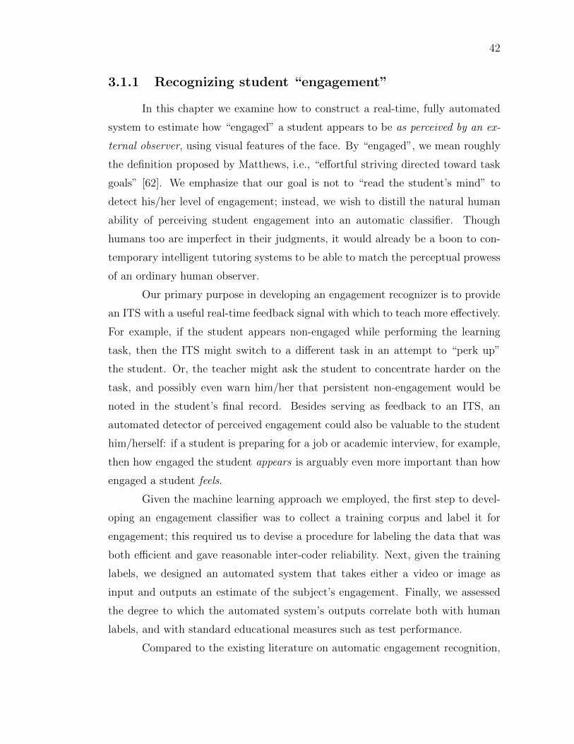
42
3.1.1 Recognizing student “engagement”
In this chapter we examine how to construct a real-time, fully automated
system to estimate how “engaged” a student appears to be as perceived by an ex-
ternal observer, using visual features of the face. By “engaged”, we mean roughly
the definition proposed by Matthews, i.e., “effortful striving directed toward task
goals” [62]. We emphasize that our goal is not to “read the student’s mind” to
detect his/her level of engagement; instead, we wish to distill the natural human
ability of perceiving student engagement into an automatic classifier. Though
humans too are imperfect in their judgments, it would already be a boon to con-
temporary intelligent tutoring systems to be able to match the perceptual prowess
of an ordinary human observer.
Our primary purpose in developing an engagement recognizer is to provide
an ITS with a useful real-time feedback signal with which to teach more effectively.
For example, if the student appears non-engaged while performing the learning
task, then the ITS might switch to a different task in an attempt to “perk up”
the student. Or, the teacher might ask the student to concentrate harder on the
task, and possibly even warn him/her that persistent non-engagement would be
noted in the student’s final record. Besides serving as feedback to an ITS, an
automated detector of perceived engagement could also be valuable to the student
him/herself: if a student is preparing for a job or academic interview, for example,
then how engaged the student appears is arguably even more important than how
engaged a student feels.
Given the machine learning approach we employed, the first step to devel-
oping an engagement classifier was to collect a training corpus and label it for
engagement; this required us to devise a procedure for labeling the data that was
both efficient and gave reasonable inter-coder reliability. Next, given the training
labels, we designed an automated system that takes either a video or image as
input and outputs an estimate of the subject’s engagement. Finally, we assessed
the degree to which the automated system’s outputs correlate both with human
labels, and with standard educational measures such as test performance.
Compared to the existing literature on automatic engagement recognition,

43
the main contributions of this work are the following:
1. We propose and execute a procedure for annotating training data for a sub-
jective emotional state such as “engagement” and evaluate it in terms of
inter-coder reliability over different timescales of labeling.
2. We propose and implement an architecture for recognizing not just binary
presence/absence, but also the real-valued degree to which a student appears
to be engaged. On the binary task, the automated system matches, and in
some cases slightly outperforms, human accuracy. On the real-valued task,
the automated system shows reasonably high accuracy compared to human
levels.
3. We show that perceived engagement, whether by a human observer or the
automated system, correlates with student test performance.
4. We analyze how human observers make their decisions as to what constitutes
each level of engagement.
This chapter is structured as follows: We first briefly review related work
in Section 3.2. Next, in Section 3.3 we describe the training set that we collected
as well as how we annotated it. Then, in Section 3.4, we propose a reasonable
architecture of an automated engagement recognition system, implement it, and
examine the most important parameters in terms of system accuracy. In Section
3.6 we examine the correlation between engagement estimates and other objec-
tive learning measurements. Finally in Section 3.7 we analyze the most important
sources of error in the current system and suggest ways for creating better engage-
ment classifiers in the future.
3.2 Related work
Student “engagement” has consistently been identified by the intelligent tu-
toring systems community as being a key affective state relevant to learning, and
hence recognizing it automatically could help to improve the effectiveness of au-
tomated teaching. Engagement recognition is also of interest to the human-robot

44
interaction and human-computer interaction communities. Previous research on
automatic student engagement recognition differs principally in how “engagement”
is defined and also through what sensors and methods it is recognized. In terms
of definition, there are four main categories: neurological and physiological ap-
proaches, self-report, external observation, and task performance.
From a neuroscience perspective, engagement might be defined in terms of
activation of particular brain regions known to modulate attention and alertness
[23]. It may then be possible to estimate the student’s engagement using elec-
troencephalography (EEG) or other neuroimaging technique, as was investigated
by [59, 70]. Physiological sensors too may facilitate engagement recognition if they
can accurately measure physiological arousal, including blood pressure, of the stu-
dent [18]. While such neurological and physiological approaches arguably drive as
close as possible to a “gold standard” of engagement, it is possible that under-
standing the exact neural or physiological basis of attention and engagement is a
much harder problem than recognizing a “softer” form of engagement defined, for
example, in terms of self-report or task performance.
More common in the ITS community are the other kinds of engagement
definitions: Engagement as defined by self-report is how engaged the student re-
ports him/herself to be. The self-reported engagement score can be collected in
an “emote aloud” fashion [28], or it could be collected after the learning task in a
survey. Such surveys need not directly ask the student explicitly how “engaged”
he/she feels but could instead map from the survey responses into an engage-
ment measure, e.g., using factor analysis [62]. Given the self-reported engagement
scores, one can attempt to recognize engagement automatically using facial ex-
pression analysis [63], EEG [39], or physiological sensors such as respiration, heart
rate, and skin conductivity sensors [33].
While students themselves have probably more direct access to their own
emotions than anyone else, it is not always practical to ask students how engaged
they feel. Moreover, a student may feel embarrassed saying he was “very non-
engaged” and may sometimes give inaccurate reports. An alternative measure of
engagement is to ask an external observer how engaged the student appears to be

45
based on live or recorded video of the student in the learning environment, com-
bined perhaps with synchronized information on the student’s task performance.
Given this definition of engagement, similar kinds of sensors and recognition ap-
proaches as for self-report can be applied to the automatic recognition problem,
including facial expression analysis [99, 29, 63], posture analysis [75, 99], or EEG.
Finally, some engagement recognition systems treat “engagement” as a la-
tent state that affects the student’s accuracy and perhaps response time in the
learning task. For instance, a “non-engaged” student might be defined as a stu-
dent who simply guesses randomly when answering a question. Using probabilistic
inference, an ITS can estimate the student’s engagement level at run-time by as-
sessing how well the student’s recent task performance can be explained by an
“engaged” student compared to a “non-engaged” student [12, 46]. This technique
has been dubbed “engagement tracing” [12], which is an allusion to the standard
“knowledge tracing” technique in many ITS [49]. Estimating engagement in this
manner does not even require any kind of “affective sensors” such as a web camera
at all – engagement can be estimated using just the student’s task performance.
However, it is also possible that, by additionally harnessing affective sensors, a
more accurate estimate of the student’s engagement level could be obtained more
quickly.
In the present study, we focus on automatically recognizing the appearance
of a student’s “engagement” level, as defined by external observers, using a web
camera and automatic face analysis methods.
3.3 Dataset collection and annotation for an au-
tomatic engagement classifier
Given our goal to train an automatic engagement recognizer that can ap-
proximate human judgments of how engaged a student appears, it is necessary to
collect a training dataset. Our particular goal is to develop a system that can
provide useful real-time observations to an intelligent tutoring system; hence, it
makes sense to collect data from a setting in which students are interacting with

46
one.
The data for this study were collected from 34 undergraduate students who
participated in a 2010-2011 “Cognitive Games” experiment whose purpose was
to measure the importance to teaching of seeing the student’s face [97]. In that
experiment, video and synchronized task performance data were collected from
subjects interacting with cognitive skills training software. Cognitive skills train-
ing has generated substantial interest in recent years; the goal is to boost students’
academic performance by first improving basic skills such as memory, processing
speed, and logic and reasoning. A few prominent such systems include Brainskills
(by Learning RX [54]) and FastForWord (by Scientific Learning [77]). The Cog-
nitive Games experiment utilized custom-built cognitive skills training software,
reminiscent of Brainskills, that was installed on an Apple iPad. A webcam was
used to videorecord the students; it was placed immediately behind the iPad and
aimed directly at the student’s face. The software consisted of three games – Set
(very similar to the classic card game), Remember, and Sum – that trained logi-
cal, reasoning, perceptual, and memory skills. The dependent variables during the
2010-2011 experiment were pre- and post-test performance on the Set game.
Experimental data for the engagement study in this chapter were taken
from 34 subjects from two pools: (a) the 26 subjects who participated in the
Spring 2011 version of the Cognitive Games study at a Historically Black Col-
lege/University (HBCU) in the southern United States. All of these subjects were
African-American, and 20 were female. Additional data were collected from (b) the
8 subjects who participated in the Summer 2012 version of the Cognitive Games
study at a university in California (UC), all of whom were either Asian-American
or Caucasian-American, and 5 of whom were female. For the present study, the
HBCU data served as the primary data source for training and testing the en-
gagement recognizer. The UC dataset allowed us to assess how well the trained
system would generalize to subjects of a different race – a known issue in modern
computer vision systems.
In the experimental setup, each subject sat in a private room and played the
cognitive skills software either alone or together with the experimenter. The iPad
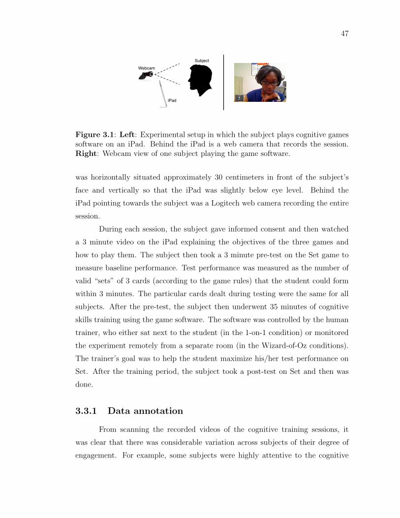
47
iPad
Webcam
Subject
Figure 3.1: Left: Experimental setup in which the subject plays cognitive gamessoftware on an iPad. Behind the iPad is a web camera that records the session.Right: Webcam view of one subject playing the game software.
was horizontally situated approximately 30 centimeters in front of the subject’s
face and vertically so that the iPad was slightly below eye level. Behind the
iPad pointing towards the subject was a Logitech web camera recording the entire
session.
During each session, the subject gave informed consent and then watched
a 3 minute video on the iPad explaining the objectives of the three games and
how to play them. The subject then took a 3 minute pre-test on the Set game to
measure baseline performance. Test performance was measured as the number of
valid “sets” of 3 cards (according to the game rules) that the student could form
within 3 minutes. The particular cards dealt during testing were the same for all
subjects. After the pre-test, the subject then underwent 35 minutes of cognitive
skills training using the game software. The software was controlled by the human
trainer, who either sat next to the student (in the 1-on-1 condition) or monitored
the experiment remotely from a separate room (in the Wizard-of-Oz conditions).
The trainer’s goal was to help the student maximize his/her test performance on
Set. After the training period, the subject took a post-test on Set and then was
done.
3.3.1 Data annotation
From scanning the recorded videos of the cognitive training sessions, it
was clear that there was considerable variation across subjects of their degree of
engagement. For example, some subjects were highly attentive to the cognitive

48
games almost the entire time, whereas one subject literally fell asleep during the
experiment. There was also variation within subjects; for instance, one subject
who usually appeared highly engaged spent a few seconds looking away from the
iPad while answering his cellular phone.
Given these recorded videos, the next step was to annotate (label) them for
“engagement”. Since our goal was to build an engagement recognizer to estimate
how engaged the student appears to be, we organized a team of labelers, consisting
of undergraduate and graduate students from computer science, cognitive science,
and psychology from the two universities where data were collected. These la-
belers viewed and rated the videos for the appearance of engagement. In pilot
experimentation we tried three different approaches to labeling:
1. Watching video clips and giving continuous engagement labels by adjusting
a “dial” (in practice, just the Up/Down arrow keys).
2. Watching video clips and giving a single number to rate the entire video.
3. Viewing static images and giving a single number to rate the entire video.
We found approach (1) very difficult to execute in practice. One problem was
the tendency to habituate to each subject’s recent level of engagement, and to
adjust the current rating relative to that subject’s average engagement level of
the recent past. This could yield labels that are not directly comparable between
subjects or even within subjects. Another problem was how to rate short events,
e.g., brief eye closure or looks to the side: should these brief moments be labeled as
“non-engagement”, or should they be overlooked as normal behavior if the subject
otherwise appears highly engaged? Finally, it was difficult to provide continuous
labels that were synchronized in time with the video; proper synchronization would
require first scanning the video for interesting events, and then re-watching it and
carefully adjusting the engagement up or down at each moment in time. We found
the labeling task was easier using approaches (2) and (3), provided that clear
instructions were given as to what constitutes “engagement”.

49
HBCU
1 2 3 4
UC
Figure 3.2: Mean faces images across either the HBCU (top) or UC (bottom)dataset for each of the four engagement levels.
3.3.2 Engagement categories and instructions
Given the approach of giving a single engagement number to an entire video
clip or image, we decided on the following approximate scale to rate engagement:
1: Not engaged at all – e.g., looking away from computer and obviously not
thinking about task, eyes completely closed.
2: Nominally engaged – e.g., eyes barely open, clearly not “into” the task.
3: Engaged in task – student requires no admonition to “stay on task”.
4: Very engaged – student could be “commended” for his/her level of engage-
ment in task.
X: The clip/frame was very unclear, or contains no person at all.
Example images and mean face images for each engagement level are shown in
Figures 3.3 and 3.2, respectively.
Labelers were instructed to label clips/images for “How engaged does the
subject appear to be?” The key here is the word appear – we purposely did
not want labelers to try to infer what was “really” going on inside the students’
minds because this left the labeling problem too open-ended. This has the con-
sequence that, if a subject blinked, then he/she was labeled as very non-engaged

50
Engagement = 1
Engagement = 2
Engagement = 3
Engagement = 4
Figure 3.3: Sample faces for each engagement level from the HBCU subjects. Allsubjects gave written consent to publication of their face images.

51
(Engagement = 1) because, at that instant, he/she appeared to be non-engaged. In
practice, we found that this made the labeling task clearer to the labelers and still
yielded informative engagement labels. If the engagement scores of multiple frames
are averaged over the course of a video clip (see Section 3.3.4), momentary blinks
will not greatly affect the average score anyway. In addition, labelers were told
to judge engagement based on the knowledge that subjects were interacting with
game software on an iPad directly in front of them. Any gaze around the room or
to another person (i.e., the experimenter) should be considered non-engagement
(rating of 1) because it implied the subject was not engaging with the iPad. The
goal here was to help the system generalize to a variety of settings where students
should be looking directly in front of them.
3.3.3 Timescale
An important variable in annotating video is the timescale at which labeling
takes place. For approach (2), we experimented with two different time scales: clips
of 60 sec and clips of 10 sec. Approach (3) (single images) can be seen as the lower
limit of the length of a video clip. In a pilot experiment we compared these three
approaches (two timescales for video, plus single images) for inter-coder reliability.
As performance metric we used Cohen’s κ averaged over all labelers in a leave-
one-labeler-out fashion (see Appendix). Since the engagement labels belong to an
ordinal scale and are not simply categories, we used a weighted κ with quadratic
weights to penalize label disagreement.
For the 60 sec labeling task, all the video sessions (∼ 45 minutes/subject)
from the HBCU subjects were watched from start to end in 60 sec clips, and
labelers entered a single engagement score after viewing each clip. For the 10 sec
labeling task, 505 video clips of 10 sec each were extracted at random timepoints
from the session videos and shown to the labelers in random (in terms of both
time and subject) order. Between the 60 sec clips and the 10 sec labeling tasks,
we found the 10 sec labeling task more intuitive. When viewing the longer clips, it
was difficult to know what label to give if the subject appeared non-engaged early
on but appeared highly engaged at the end. The inter-coder reliability of the 60

52
sec clip labeling task was κ = 0.39 (across two labelers); for the 10 sec clip labeling
task κ = 0.68.
For approach (3), we created custom labeling software in which labelers an-
notated batches of 100 images each. The images for each batch were video frames
extracted at random timepoints from the session videos. Each batch contained a
random set of images spanning multiple timepoints from multiple subjects. Label-
ers rated each image individually but could view many images and their assigned
labels simultaneously on the screen. The labeling software also provided a Sort
button to sort the images in ascending order by their engagement label. In prac-
tice, we found this to be an intuitive and efficient method of labeling images for
the appearance of engagement. The inter-coder reliability for image-based label-
ing was κ = 0.56. If we exclude the single labeler with the lowest inter-subject
agreement, then κ = 0.60.
In terms of timescale, it seems that short video clips give the best reliability
of the three timescales. However, the reliability of image-based labeling is not far
behind that of the 10 sec video clips. Furthermore, it is possible that, if we average
together the labels for individual image frames that were sampled from consecutive
timepoints from a single video, then the reliability of these averaged sets of frames
might be even higher. We examined this issue in the subsection below.
3.3.4 Static pixels versus dynamics
One interesting question is how much information about students’ engage-
ment is captured in the static pixels of the individual video frames compared to
the dynamics of the motion. We conducted a pilot study to examine this question.
In particular, we randomly selected 120 video clips (10 sec each) across many sub-
jects and split each clip into 40 frames spaced 0.25 sec apart. These frames were
then shuffled both in time and across subjects. A human labeler then labeled these
image frames for the appearance of engagement, as described in “approach (3)” of
Section 3.3.1. Finally, the engagement values assigned to all the frames for a par-
ticular clip were reassembled and averaged; this average served as an estimate of
the “true” engagement score given by that same labeler when viewing that video

53
clip as described in “approach (2)” above. We found that, with respect to the
true engagement scores, the estimated scores gave a κ = 0.78, and the fraction of
explained variance was 0.72. Though not perfect, this “reconstruction” accuracy
is quite high, and suggests that most of the information about the appearance of
engagement is contained in the static pixels, not the motion per se.
In addition to computing the reconstruction accuracy, we also examined the
video clips in which the reconstructed engagement scores differed the most from
the true scores. In particular, we ranked the 120 labeled video clips in decreasing
order of absolute deviation of the estimated label (by averaging the frame-based
labels) from the “true” label given to the video clip viewed as a whole. We then
examined these clips and attempted to explain the discrepancy:
In the first clip (greatest absolute deviation), the subject was swaying her
head from side to side as if listening to music (although she was not). It is likely
that the coder treated this as non-engaged behavior. Clearly, this is a behavior
that cannot be easily captured from static frame judgments – it requires some
means of recognizing the dynamics. However, it was also an anomalous case.
In the second clip, the subject turned his head to the side to look at the
experimenter, who was talking to him for several seconds. In the frame-level
judgments, this was perceived as off-task, and hence non-engaged behavior; this
corresponds to the instructions given to the coders that they rate engagement under
the assumption that the subject should always be looking towards the iPad. For
the video clip label, however, the coder judged the student to be highly engaged
because he was intently listening to the experimenter. This is an example of
inconsistency on the part of the coder as to what constitutes engagement and does
not necessarily indicate a problem with splitting the clips into frames.
Finally, in several clips the subjects shifted their eye gaze downward several
times to look at the bottom of the iPad screen. At a frame level, it was difficult
to distinguish the subject looking at the bottom of the iPad from the subject
looking to his/her own lap, which would be considered non-engagement. This is
an example of a student behavior that can be more accurately labeled from video
clips compared to frames. In most videos, however, the mislabeling of the subjects’
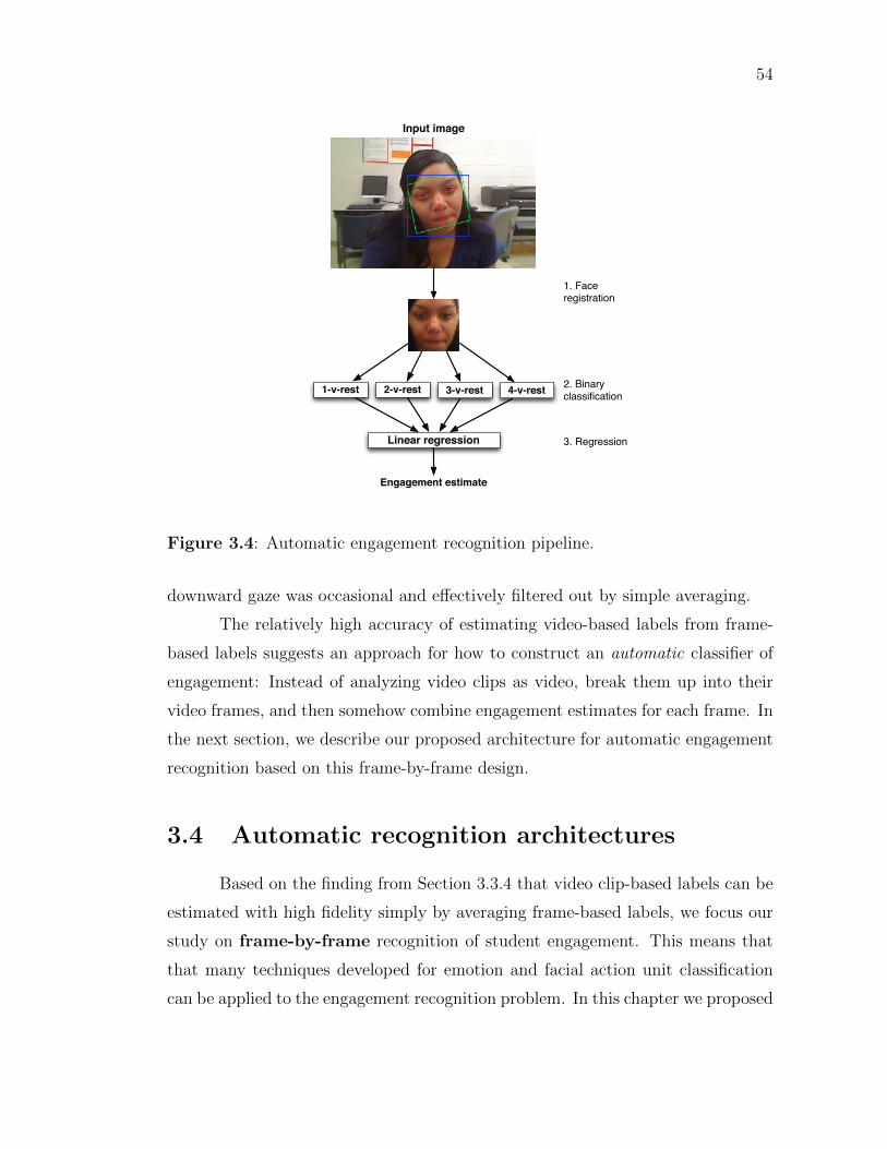
54
Input image
1-v-rest 2-v-rest 3-v-rest 4-v-rest
Linear regression
Engagement estimate
1. Face registration
2. Binary classification
3. Regression
Figure 3.4: Automatic engagement recognition pipeline.
downward gaze was occasional and effectively filtered out by simple averaging.
The relatively high accuracy of estimating video-based labels from frame-
based labels suggests an approach for how to construct an automatic classifier of
engagement: Instead of analyzing video clips as video, break them up into their
video frames, and then somehow combine engagement estimates for each frame. In
the next section, we describe our proposed architecture for automatic engagement
recognition based on this frame-by-frame design.
3.4 Automatic recognition architectures
Based on the finding from Section 3.3.4 that video clip-based labels can be
estimated with high fidelity simply by averaging frame-based labels, we focus our
study on frame-by-frame recognition of student engagement. This means that
that many techniques developed for emotion and facial action unit classification
can be applied to the engagement recognition problem. In this chapter we proposed

55
a 3-stage pipeline (see Figure 3.4):
1. Face registration: the face and facial feature positions are localized in the
image; the face box coordinates are computed; and the face patch is cropped
from the image [57]. We experimented with 36 × 36 and 48 × 48 pixel face
resolution.
2. The cropped face patch is classified by four binary classifiers, one for each
engagement category e ∈ {1, 2, 3, 4}.
3. The outputs of the binary classifiers are fed to a regressor to estimate the
image’s engagement level.
Stage (1) is standard for automatic face analysis tools, and our particular approach
is described in [57]. Stage (2) is discussed in the next subsection, and stage (3) is
discussed in Section 3.4.8.
3.4.1 Binary classification
We trained four binary classifiers of engagement – one for each of the four
levels described in Section 3.3.1. The task of each of these classifiers is to dis-
criminate an image (or video frame) that belongs to engagement level e from an
image that belongs to some other engagement level e′ 6= e. We call these detectors
1-v-rest, 2-v-rest, etc. We compared three commonly used and demonstrably ef-
fective feature type + classifier combinations from the automatic facial expression
recognition literature:
• GentleBoost with Box Filter features (GB(BF)): this is the approach pop-
ularized Viola and Jones in [92] for face detection.
• Support vector machines with Gabor Energy Filters (SVM(GEF)): this
approach has achieved some of the highest accuracies in the literature for
facial action and basic emotion classification [57].
• Multivariate logistic regression with expression outputs from the Computer
Expression Recognition Toolbox [57] (MLR(CERT)): here, we attempt to

56
harness an existing automated system for facial expression analysis to train
the student engagement classifiers.
We describe each approach in more detail below:
GB(BF)
Box Filter (BF) features were shown in [95] to be highly effective for auto-
matic smile detection. At run-time, BF features are extremely fast to extract using
the “integral image” technique [92]. At training time, however, the number of BF
features relative to the image resolution is very high compared to other image
representations (e.g., a Gabor decomposition), which can lead to overfitting. BF
features are typically combined with a boosted classifier such as Adaboost [36] or
GentleBoost (GB) [37], which performs both feature selection during training and
actual classification at run-time. In our GentleBoost implementation, each weak
learner consists of a non-parametric regressor smoothed with a Gaussian kernel
of bandwidth σ, to estimate the log-likelihood ratio of the class label given the
feature value. Each GentleBoost classifier was trained for 100 boosting rounds.
For the features, we included 6 types of Box Filters in total, comprising two-,
three-, and four-rectangle features similar to those used in [92], and an additional
two-rectangle “center-surround” feature.
SVM(GEF)
Gabor Energy Filters (GEF) [65] are bandpass filters with a tunable spa-
tial orientation and frequency. They model the complex cells of the primate’s
visual cortex. Gabor Energy Filters have a proven record in a wide variety of face
processing applications, including face recognition [52] and facial expression recog-
nition [57]. In machine learning applications GEF features are often classified by
a soft-margin linear support vector machine (SVM) with parameter C specifying
how much misclassified training examples should penalize the objective function.
In our implementation, we applied a “bank” of 40 Gabor Energy Filters consisting
of 8 orientations (spaced at 22.5deg intervals) and 5 spatial frequencies spaced at
half-octaves.

57
MLR(CERT)
The Facial Action Coding System [32] is a comprehensive framework for
objectively describing facial expression in terms of Action Units, which measure
the intensity of over 40 distinct facial muscles. Manual FACS coding has previously
been used to study student engagement and other emotions relevant to automated
teaching [48, 63]. In our study, since we are interested in automatic engagement
recognition, we employ the Computer Expression Recognition Toolbox (CERT),
which is a software tool developed by our laboratory to estimate facial action in-
tensities automatically [57]. Although the accuracies of the individual facial action
classifiers vary, we have found CERT to be useful for a variety of facial analysis
tasks, including the discrimination of real from faked pain [56], driver fatigue de-
tection [93], and estimation of students’ perception of curriculum difficulty [94].
CERT outputs intensity estimates of 20 facial actions as well as the 3-D pose of
the head (yaw, pitch, and roll). For engagement recognition we classify the CERT
outputs using multivariate logistic regression (MLR), trained with an L2 regular-
izer on the weight vector of strength α. We use the absolute value of the yaw,
pitch, and roll to provide invariance to the direction of the pose change.
Internally, CERT uses the SVM(GEF) approach described above. Since
CERT was trained on 280 subjects, which is substantially higher than the number
of subjects collected for this study, it is possible that CERT’s outputs will provide
an identity-independent representation of the students’ faces, which may boost
generalization performance.
3.4.2 Data selection
We used the following procedure to select training and testing data for each
binary classifier to distinguish e-v-rest:
1. For each of the labeled HBCU images, we considered the set of all labels
given to that image by all the labelers. If any labeler marked the frame as
X (no face, or very unclear), then the image was discarded.
2. If the minimum and maximum label given to an image differed by more than

58
1 (e.g., one labeler assigns a label of 1 and another assigns a label of 3), then
the image was discarded.
3. If the automatic face detector (from CERT [57]) failed to detect a face, or if
the largest detected face was less than 36 pixels wide (usually indicative of
a false alarm), the image was discarded.
4. Otherwise, the “ground truth” label for that image was computed by round-
ing the average label for that image (e.g., 2.4 rounds to 2; 2.5 rounds to
3). If the rounded label equalled e, then that image was considered a posi-
tive example for that classifier’s training set; otherwise, it was considered a
negative example.
In total there were 14204 frames from the HBCU dataset selected using this ap-
proach.
3.4.3 Cross-validation
We used 4-fold subject-independent cross-validation to measure the accu-
racy of each trained binary classifier. Specifically, the set of all labeled frames
was partitioned into 4 folds such that no subject appeared in more than one fold;
hence, the cross-validation estimate of performance gives a sense of how well the
classifier would perform on a novel subject on which the classifier was not trained.
3.4.4 Accuracy metric
We use the 2AFC [100] metric to measure accuracy, which expresses the
probability of correctly discriminating a positive example from a negative example
in a 2-alternative forced choice classification task. Under mild assumptions the
2AFC is equivalent to the area under the Receiver Operating Characteristics curve,
which is commonly used in the facial expression recognition literature. To assess
the machine’s accuracy relative to inter-human accuracy, we computed the 2AFC
for human labelers as well, using the same image selection criteria as described in
Section 3.4.2.

59
3.4.5 Hyperparameter selection
Each of the classifiers listed above has a hyperparameter associated with it
(either σ, C, or α). The choice of hyperparameter can impact the test accuracy sub-
stantially, and it is a common pitfall to give an overly optimistic estimate of a clas-
sifier’s accuracy by manually tuning the hyperparameter based on the test set per-
formance. To avoid this pitfall, we instead optimize the hyperparameters using only
the training set by further dividing each training set into 4 subject-independent
inner cross-validation folds in a double cross-validation paradigm. We selected
hyperparameters from the following sets of values: σ ∈ {10−2, 10−1.5, . . . , 100},C ∈ {0.1, 0.5, 2.5, 12.5, 62.5, 312.5}, and α ∈ {10−5, 10−4, . . . , 10+5}.
3.4.6 Results: binary classification
Classification results are shown in Table 3.1 for cropped face resolution
of 48 × 48 pixels. Accuracy at 36 × 36 pixel resolution was slightly lower. All
results are for subject-independent classification. From the upper table, we see that
the binary classification accuracy given by the machine classifiers is very similar
to inter-human accuracy. All of the three architectures tested delivered similar
performance averaged across the four tasks (1-v-rest, 2-v-rest, etc.). However,
MLR(CERT) performed noticeably worse for 1-v-rest, and noticeably better for
4-v-rest. As we discuss in Section 3.5, many images labeled as Engagement = 1
exhibit eye closure; in addition, Engagement = 4 can be discriminated using pose
information. It is possible that CERT’s eye closure detector is relatively inaccurate,
and in comparison the GB(BF) and SVM(Gabor) approaches are able to learn an
accurate eye closure detector from the training data themselves. On the other hand,
CERT may have an advantage in terms of pose information because CERT’s pose
detector was trained on tens of thousands of subjects.
Overall we find the results encouraging that machine classification of en-
gagement can reach inter-human levels of accuracy. However, another important
problem beyond binary classification is estimating the real-valued degree of en-
gagement, which we examine in Section 3.4.8.

60
Table 3.1: Top: Subject-independent, within-dataset (HBCU), image-based en-gagement recognition accuracy for each engagement level e ∈ {1, 2, 3, 4} using eachof the three classification architectures, along with inter-human classification ac-curacy. Bottom: Engagement recognition accuracy on a different dataset (UC)not used for training.
Accuracy (2AFC): train on HBCU, test on HBCUClassifier
Task MLR(CERT) GB(BF) SVM(Gabor) Human1-v-rest 0.8322 0.9697 0.9139 0.91322-v-rest 0.7554 0.7688 0.7109 0.67363-v-rest 0.5842 0.6107 0.6303 0.62724-v-rest 0.7011 0.6101 0.6600 0.6563Avg 0.7182 0.7398 0.7288 0.7176
Accuracy (2AFC): train on HBCU, test on UCClassifier
Task MLR(CERT) GB(BF) SVM(Gabor)1-v-rest 0.7745 0.9234 0.83072-v-rest 0.6179 0.7049 0.66783-v-rest 0.5053 0.5262 0.56964-v-rest 0.6176 0.6540 0.6965Avg 0.6288 0.7021 0.6911

61
3.4.7 Generalization to a different dataset
A well-known issue for contemporary face analysis systems is to generalize
to people of a different race from the people in the training set; in particular,
modern face detectors often have difficulty detecting people with dark skin [95]. For
our study, we collected data both at HBCU, where all the subjects were African-
American, as well as UC, where all the subjects were either Asian-American or
Caucasian-American. This gives us the opportunity to assess how well a classifier
trained on one dataset generalizes to the other. Here, we measure performance of
the binary classifiers described above that were trained on HBCU when classifying
subjects from UC.
Results are shown in Table 3.1 for each feature type and classifier combi-
nation. For GB(BF) and SVM(GEF), the degradation in performance was mild.
Interestingly, the MLR(CERT) architecture generalized the worst, even though
CERT was trained on a much larger number of subjects (several hundred, com-
pared to just 26 for this study) and outputs only a small number of features. It
is possible that the head pose features that are measured by CERT and are useful
for the HBCU dataset do not generalize to the UC dataset.
3.4.8 Regression
After performing binary classification of the input image for each engage-
ment level e ∈ {1, 2, 3, 4}, the final stage of the pipeline is to combine the classifier
outputs into a real-valued estimate of the student’s engagement. Here, as a first
implementation, we use standard linear regression using the raw binary classifier
outputs as features. Note, however, that more sophisticated methods of “averag-
ing” are possible, such as using a non-linear classification method over histograms
of frame-based engagement scores instead of simply taking the sample mean.
3.4.9 Results: regression
We chose the SVM(GEF) architecture and trained a linear regressor to map
from the four binary classifiers’ outputs to a real-valued engagement estimate.
62
Subject-independent 4-fold cross-validation accuracy, measured using Pearson’s
correlation r, was 0.50. For comparison, inter-human accuracy on the same task
was 0.71.
The fact that human accuracy approximately equal to machine accuracy
on the binary classification tasks, whereas it is higher for the regression task,
suggests that there are some images on which the binary engagement classifiers
make “egregious mistakes”, e.g., the automated system believes that a student
whom humans labeled as a 4 was a 1. In other words, the machine may make fewer
binary classification mistakes than the humans do, but the mistakes it makes are
much “worse”. We discuss this further in Section 3.7.
3.5 Reverse-engineering the human labelers
Given that our goal in this project is to recognize student engagement
as perceived by an external observer, it is interesting and instructive to analyze
how the human labelers formed their judgments. From Figure 3.3 we can see
clearly that eye closure is a strong indicator of low engagement, as are large head
pose deviations from frontal. At engagement level 2, which we call “nominally
engaged”, the subject is often resting his/her head on one hand. This is also
reflected in the slight smearing of the subject’s left cheek in the Engagement = 2
image from the HBCU subjects and more pronouncedly from the UC subjects in
Figure 3.2. Note the subtle difference between resting the head on the hand and
placing the hand in front of the face, as exhibited by the third subject from the
left in the Engagement = 4 row in Figure 3.3. The difference between groups
Engagement = 3 and Engagement = 4 is subtle but noticable, particularly in the
intensity of the subjects’ eye gaze towards the screen and possible furrowing of the
eye brow when Engagement = 4. Finally, Figure 3.3 also suggests that subjects in
Engagement = 4 lean forward slightly towards the iPad.
We can also use the weights assigned to the CERT features that were learned
by the MLR(CERT) classifiers to assess quantitatively how the human labelers
judged engagement – if the MLR weight assigned to AU 45 (eye closure) had a large

63
AU 1 AU 10
CERT feature Weightabs(Roll) −0.5659AU 10 +0.5089AU 1 −0.4430AU 45 −0.2851abs(Pitch) −0.2644
Figure 3.5: Weights associated with different Action Units (AUs) to discriminateEngagement = 4 from Engagement 6= 4, along with examples of AUs 1 and 10.Pictures courtesy of Carnegie Mellon University’s Automatic Face Analysis groupwebpage.
magnitude, for example, then that would suggest that eye closure was an important
factor in how humans labeled the dataset on which that MLR classifier was trained.
In particular, when we examine the 5 MLR weights of highest magnitude that were
learned by the 4-v-rest MLR(CERT) classifier, we obtain the results shown in
Figure 3.5. (Here, we trained a 4-v-rest classifier on all the subjects’ data because
we were not interested in cross-validation performance.) The most discriminating
feature was the absolute value of roll (in-plane rotation of the face), with which
Engagement = 4 was negatively associated (weight of −0.5659). It is possible that
the hand-resting-on-hand that is prominent for Engagement = 2 also induces roll
in the head, and that the MLR(CERT) classifier learned this trend. The second
most discriminating facial action was Action Unit 10 (upper lip raiser), which was
positively correlated with Engagement = 4; speculatively, this AU may suggest
that frustration or even annoyance at the learning task can be correlated with
high levels of engagement. AU 1 (inner brow raiser), AU 45 (eye closure), and
the absolute value of pitch (tilting of the head up and down) were also negatively
correlated with Engagement = 4.
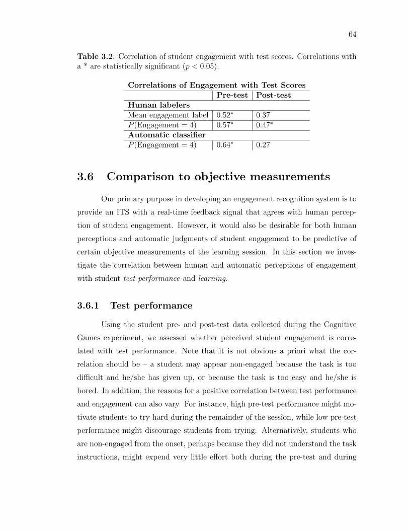
64
Table 3.2: Correlation of student engagement with test scores. Correlations witha * are statistically significant (p < 0.05).
Correlations of Engagement with Test ScoresPre-test Post-test
Human labelersMean engagement label 0.52∗ 0.37P (Engagement = 4) 0.57∗ 0.47∗
Automatic classifierP (Engagement = 4) 0.64∗ 0.27
3.6 Comparison to objective measurements
Our primary purpose in developing an engagement recognition system is to
provide an ITS with a real-time feedback signal that agrees with human percep-
tion of student engagement. However, it would also be desirable for both human
perceptions and automatic judgments of student engagement to be predictive of
certain objective measurements of the learning session. In this section we inves-
tigate the correlation between human and automatic perceptions of engagement
with student test performance and learning.
3.6.1 Test performance
Using the student pre- and post-test data collected during the Cognitive
Games experiment, we assessed whether perceived student engagement is corre-
lated with test performance. Note that it is not obvious a priori what the cor-
relation should be – a student may appear non-engaged because the task is too
difficult and he/she has given up, or because the task is too easy and he/she is
bored. In addition, the reasons for a positive correlation between test performance
and engagement can also vary. For instance, high pre-test performance might mo-
tivate students to try hard during the remainder of the session, while low pre-test
performance might discourage students from trying. Alternatively, students who
are non-engaged from the onset, perhaps because they did not understand the task
instructions, might expend very little effort both during the pre-test and during

65
the rest of the session.
Human labels
We first compared human judgments of engagement with test performance
by computing the mean engagement label over all labeled frames for each subject
in the HBCU dataset, and then correlating these mean engagement labels with
pre-test and post-test scores. The Pearson correlation between engagement and
pre-test was r = 0.52 (p < 0.05) and between engagement and post-test was
r = 0.37 (not statistically significant).
We also examined which of the 4 engagement levels was most predictive of
task performance by correlating the fraction of frames labeled as Engagement = 1,
Engagement = 2, etc., with student test performance. Only Engagement = 4
was positively correlated with pre-test (r = 0.57, p < 0.05) and post-test (r =
0.47, p < 0.05) performance. In fact, the fraction of frames for which a student
appeared to be in engagement level 4 was a better predictor than the mean en-
gagement predictor described above. All the other engagement levels e < 4 were
negatively (though non-significantly) correlated with test performance, suggesting
that Engagement = 4 is the only “positive” engagement state.
For comparison, the correlation between students’ pre-test and post-test
scores was r = 0.44 – in other words, human perceptions of student Engagement =
4 as labeled on a frame-by-frame basis is a better predictor of post-test performance
than is the student’s pre-test score.
Automatic estimates
We also computed the correlation between automatic judgments of engage-
ment and student pre- and post-test performance. Since the best predictor of test
performance from human judgments was from the fraction of frames labeled as
Engagement = 4, we focused on the output of the 4-v-rest classifier. In particular,
we correlated the fraction of frames over each subject’s entire video session that the
4-v-rest detector predicted to be a “positive” frame by thresholding with τ , where
τ is the median detector output over all subjects’ frames. In other words, frames

66
on which the detector’s output exceeded τ was considered to be a “positive” frame
for engagement level 4. The correlation with this automatic Engagement = 4 pre-
dictor and pre-test performance was 0.64 (p < 0.05); for post-test performance, it
was r = 0.27 (not statistically significant).
3.6.2 Learning
In addition to raw test performance, we also examined correlations between
engagement and learning. One simple definition of “learning” is post-test minus
pre-test scores. The correlation between mean engagement for each subject, as
labeled by humans, and post-test minus pre-test, was practically 0. The correlation
between fraction of frames labeled as Engagement = 4 and post-test minus test
was 0.08 and was not statistically significant.
On the other hand, the simple post-test minus pre-test measure does not
account for possible ceiling effects in testing – it is possible that increasing test
performance from, say, 10 to 12 is much harder than from 0 to 2. Hence, as an
alternative measure of learning, we also examined exp(post-test) minus exp(pre-
test) which gives a larger weight to score increases starting from a higher baseline.
Using this new learning metric, the correlation between mean label and learning is
r = 0.32, and the correlation between fraction of frames labeled as Engagement = 4
and learning was r = 0.37. Though neither correlation is statistically significant,
these results still mildly support the possibility of a ceiling effect in the Set task
on which students were tested.
3.7 Error analysis
In this section we consider some of the most important sources of error in the
automated engagement detector. Identifying the important classes of incorrectly
classified images may suggest avenues for further research that will help to improve
future engagement recognition systems.
We examined the most egregious (i.e., largest absolute difference between
human labels and machine-estimated label) mistakes made by the automatic en-

67
Figure 3.6: Representative images that the automated engagement detector mis-classified. Left: inaccuracy face or facial feature detection. Middle: Thick-rimmed eyeglasses that was incorrectly interpreted as eye closure. Right: Subtledistinction between looking down and eye closure.
gagement regressor (see Section 3.4.8) within the two cross-validation folds in which
accuracy was the lowest. There were three chief sources of errors: (1) The face
detector or facial feature detector did not accurately find the face or facial features
(Figure 3.6 left). Given an inaccurate facebox, it is natural that all downstream
processing, including engagement recognition, can be highly inaccurate. (2) The
presence of thick-rimmed eyeglasses can skew the output of the eye closure detec-
tor, which is a key input to the classifier of Engagement=1. One female subject
(Figure 3.6 middle) in particular wore such eyewear and though the human la-
bels indicated she was highly engaged, the automatic classifier believed her eyes
were mostly closed. (3) It was sometimes difficult to distinguish a subject looking
down to the bottom of the iPad from looking completely down to his/her lap in
a non-engaged manner (Figure 3.6 right). This resulted in many frames being
misclassified for one male subject in particular. Interestingly, if we re-compute the
system’s accuracy after removing this subject from the test set, then the cross-
validation accuracy increases substantially to r = 0.56.
Problems (1) and (2) should likely diminish as face and facial feature detec-
tors become more accurate and robust to different head poses, eyewear, and skin
color. Problem (3) may possibly improve with a larger training set.

68
3.8 Conclusion
We have presented an architecture for an automatic recognition system of
how “engaged” a student who is interacting with an intelligent tutoring system
appears to be. Analysis of human engagement labels suggests that most of the
information is captured from static pixels, not the video dynamics, so that frame-
by-frame analysis is possible.
On binary classification tasks (e.g., Engagement = 4 versus Engagement 6=4), the machine classifier’s accuracy is comparable to humans’. On the real-valued
regression task, machine accuracy (Pearson r = 0.50) is reasonable but needs
improvement compared to inter-human agreement (r = 0.71). Analysis of the most
egregious classification mistakes suggest that accuracy can be improved through
more accurate face and facial feature detection as well as greater robustness to
artifacts such as eyeglasses. In addition, when we consider that modern expression
recognition systems are typically trained in hundreds [57] if not thousands [95]
of subjects, it seems reasonable to assume that higher accuracy can be achieved
by growing the training set. Even at the current accuracy levels, however, the
automatic engagement detector developed in this study is already predictive of
objective measurements such as test performance, and it may serve as a useful
feedback signal to automated teaching systems.
3.9 Appendix: calculating inter-human accuracy
The automatic classifiers we develop for this chapter are trained on and
evaluated against the average label, across all human labelers, given to each image.
In order to enable a fair comparison between inter-human accuracy and machine-
human accuracy, we assess the accuracy (using Cohen’s κ, Pearson’s r, or the
2AFC metric) of each human labeler l by comparing his/her labels to the average
label, over all other labelers l′ 6= l, given to each image. We then average the
individual accuracy scores over all labelers and report this as the inter-human
reliability. Note that this “leave-one-labeler-out” agreement is typically higher
than the average pair-wise agreement.

69
3.10 Acknowledgments
Support for this work was provided by NSF grants IIS 0968573 SOCS, SBE-
0542013, and CNS-0454233, and by the Temporal Dynamics of Learning Center
(TDLC) at UCSD.
Chapter 3, in full, is currently being prepared for submission for publication
of the material. Jacob Whitehill, Zewelanji Serpell, Yi-Ching Lin, Aysha Foster,
and Javier Movellan. The dissertation author was the primary investigator and
author of this material.

Chapter 4
Measuring the Perceived
Difficulty of a Lecture Using
Automatic Facial Expression
Recognition
Abstract : In this chapter we show how automatic real-time facial expres-
sion recognition can be used to estimate the difficulty level, as perceived by an
individual student, of a delivered lecture. We also show that facial expression is
predictive of an individual student’s preferred rate of curriculum presentation at
each moment in time. On a video lecture viewing task, training on less than two
minutes of recorded facial expression data and testing on a separate validation set,
our system predicted the subjects’ self-reported difficulty scores with mean accu-
racy of 0.42 (Pearson r) and their preferred viewing speeds with mean accuracy of
0.29. Our techniques are fully automatic and have potential applications for both
intelligent tutoring systems (ITS) and standard classroom environments.
70

71
4.1 Introduction
One of the fundamental challenges faced by teachers – whether human or
robot – is determining how well his/her students are receiving a lecture at any given
moment. Each individual student may be content, confused, bored, or excited by
the lesson at a particular point in time, and one student’s perception of the lecture
may not necessarily be shared by his/her peers. While explicit feedback signals
to the teacher such as a question or a request to repeat a sentence are useful,
they are limited in their effectiveness for several reasons: If a student is confused,
he may feel embarrassment in asking a question. If the student is bored, it may
be inappropriate to ask the teacher to speed up the rate of presentation. Some
research has also shown that students are not always aware of when they need help
[2]. Finally, even when students do ask questions, this feedback may, in a sense,
come too late – the student may already have missed an important point, and the
teacher must spend lesson time to clear up the misunderstanding.
If, instead, the student could provide feedback at an earlier time, perhaps
even subconsciously, then moments of frustration, confusion, and even boredom
could potentially be avoided. Such feedback is particularly useful for automated
tutoring systems. For example, an interactive tutoring system could dynamically
adjust the speed of the instruction to increase when the student’s understanding
is solid and to slow down during an unfamiliar topic.
In this chapter we explore one such kind of feedback signal based on au-
tomatic recognition of a student’s facial expression. Recent advances in the fields
of pattern recognition, computer vision, and machine learning have made auto-
matic facial expression recognition in real-time a viable resource for intelligent
tutoring systems (ITS). The field of ITS has already begun to make use of this
technology, especially for the task of predicting the student’s affective state (e.g.,
[47, 72, 27, 76]). This chapter investigates the potential usefulness of automatic
expression recognition for two different tasks: (1) measuring the difficulty as per-
ceived by students of a delivered lecture, and (2) determining the preferred speed
at which lesson material should be presented. To this end, we conducted a pilot
experiment in which subjects viewed a video lecture at an adjustable speed while

72
their facial expressions were recognized automatically and recorded. Using the
“difficulty” scores that the subjects report, the correlations between facial expres-
sion and difficulty, and between facial expression and preferred viewing speed, can
be assessed.
The rest of this chapter is organized as follows: In Section 4.2, we briefly
describe the automatic expression recognition system that we employ in our study.
Section 4.3 describes the experiment we perform on human subjects, and Sec-
tion 4.4 presents the results. We end with some concluding remarks about facial
expression recognition for ITS.
4.2 Facial Expression Recognition
Facial expression is one of the most powerful and immediate means for hu-
mans to communicate their emotions, cognitive states, intentions, and opinions to
each other [31]. In recent years, researchers have made considerable progress in
developing automatic expressions classifiers [87, 11, 69]. Some expression recog-
nition systems classify the face into the set of “prototypical” emotions such as
happy, sad, angry, etc. [55]. Others attempt to recognize the individual muscle
movements that the face can produce [10] in order to provide an objective descrip-
tion of the face. The best known psychological framework for describing nearly
the entirety of facial movements is the Facial Action Coding System (FACS) [32].
4.2.1 FACS
FACS was developed by Ekman and Friesen as a method to code facial ex-
pressions comprehensively and objectively [32]. Trained FACS coders decompose
facial expressions in terms of the apparent intensity of 46 component movements,
which roughly correspond to individual facial muscles. These elementary move-
ments are called action units (AU) and can be regarded as the “phonemes” of
facial expressions. Figure 4.1 illustrates the FACS coding of a facial expression.
The numbers identify the action unit, which approximately corresponds to one
facial muscle; the letter (A-E) identifies the level of activation.

73
Figure 4.1: Example of comprehensive FACS coding of a facial expression. Thenumbers identify the action unit, which approximately corresponds to one facialmuscle; the letter (A-E) identifies the level of activation.
4.2.2 Automatic Facial Expression Recognition
We use the automatic facial expression recognition system presented in [10]
for our experiments. This machine learning-based system analyzes each video
frame independently. It first finds the face, including the location of the eyes,
mouth, and nose for registration, and then employs support vector machines and
Gabor energy filters for expression recognition. The version of the system employed
here recognizes the following AUs: 1 (inner brow raiser), 2 (outer brow raiser), 4
(brow lowerer), 5 (upper eye lid raiser), 9 (nose wrinkler), 10 (upper lip raiser), 12
(lip corner puller), 14 (dimpler), 15 (lip corner depressor), 17 (chin raiser), 20 (lip
stretcher), and 45 (blink), as well as a detector of social smiles.
4.3 Experiment
The goal of our experiment was to assess whether there exist significant cor-
relations between certain AUs and the perceived difficulty as well as the preferred
viewing speed of a video lecture. To this end, we composed a short composite
“lecture” video consisting of seven individual movie clips about a disparate range
of topics. The individual clips were excerpts taken from public-domain videos from
the Internet. In order, they were:

74
Figure 4.2: Representative video frames from each of the 7 video clips containedin our “lecture” movie.
1. An introductory university physics lecture (46 sec).
2. A university lecture on Sigmund Freud (36 sec).
3. A soundless tutorial on Vedic mathematics (46 sec).
4. A university lecture on philosophy (20 sec).
5. A barely audible sound clip (with a static picture backdrop) of Sigmund
Freud (16 sec).
6. A teenage girl speaking quickly while telling a humorous story (21 sec).
7. Another excerpt on physics taken from the same source as the first clip (15
sec).
Representative video frames of all 7 video clips are shown in Figure 4.2.
4.3.1 Procedure
Each subject performed the following tasks in order:
1. Watch the video lecture. The playback speed could be adjusted contin-
uously by the subject. Facial expression data were recorded.
2. Take the quiz. The quiz consisted of 6 questions about specific details of
the lecture.
3. Self-report on the difficulty. The video lecture was re-played at a fixed
speed of 1.0.

75
For watching the lecture at an adjustable speed we created a special viewing
program in which the user can press Up to increase the speed, Down to decrease the
speed, and Left to rewind by two seconds. Rewinding the video also set the speed
back to the default rate (1.0). The video player was equipped with an automatic
pitch equalizer so that, even at high speeds, the lecture audio was reasonably
intelligible. Subjects practiced using the speed controls on a separate demo video
prior to beginning the actual study. In order to encourage subjects to use their
time efficiently and thus to avail themselves of the speed control, we informed them
prior to the first viewing that they would take a quiz afterwards, and that their
performance on the quiz would be penalized by the amount of time they needed to
watch the video. We also started a visible, automatic “shut-off” timer when they
started watching the lecture to give the impression of additional time pressure. In
actuality, the timer provided enough time to watch the whole lecture at normal
speed, and the quiz was never graded – these props were meant only to encourage
the subjects to modulate the viewing speed efficiently.
While watching the video lecture for the first time, the subject’s facial ex-
pression data were recorded automatically through a standard Web camera using
the automatic face and expression recognition system described in [10]. The ex-
periment was performed in an ordinary office environment inside our laboratory
without any special lighting conditions. After watching the video and taking the
quiz, subjects were then informed that they would watch the lecture for a second
time. During the second viewing, subjects could not change the speed (it was
fixed at 1.0), but they instead rated frame-by-frame how difficult they found the
movie to be on an integral scale of 0 to 10 using the keyboard (A for “harder”,
Z for “easier”). This form of continuous audience response labeling was originally
developed for consumer research [34]. Subjects were told to consider both acoustic
as well as conceptual difficulty when assessing the difficulty of the lecture material.
Facial expression information was not collected during the second viewing.
In our experimental design, the fact that subjects adjusted the viewing
speed of the lecture video while viewing it may have affected their perception of how
difficult the lecture was to understand. Our reason for designing the experiment
76
in this way was to capture both speed control and difficulty information from all
subjects. However, we believe that the ability to adjust the speed of the lecture
would, if anything, cause the self-reported Difficulty values to be more “flat,” thus
increasing the challenge of the prediction task (predict Difficulty from Expression).
4.3.2 Human Subjects
Eight subjects (five female, three male) participated in our pilot experiment.
Subjects ranged in age from early 20’s to mid 30’s and were either undergraduate
students, graduate students, or administrative or technical staff at our university.
Five were native English speakers (American), and three were non-native (one was
Northern European, one was Southern European, and one was East Asian). Each
subject was paid $15 for his/her participation, which required about 20 minutes
in total.
None of the subjects was aware of the purpose of the study or that facial
expression data would be captured. Prior to starting the experiment, subjects
were informed only that they would be watching a video at a controllable speed
and that they would be quizzed afterward. They were not informed of rating
the difficulty of the experiment or of watching the video at second time until
after the quiz. Subjects were not requested to restrict head movement in any
way (though all remained seated throughout the entire video lecture), and the
resulting variability in head pose, while presenting no fundamental difficulty for
our expression recognition system, may have added some amount of noise. Due to
the need to manually adjust the viewing angle of the camera for facial expression
recording, it is possible that subjects inferred that their facial behavior would be
analyzed.
4.3.3 Data Collection and Processing
While the subjects watched the video, their faces were analyzed in real-time
using the expression recognition system presented in [10]. The output of 12 action
unit detectors (AUs 1, 2, 4, 5, 9, 10, 12, 14, 15, 17, 20, 45) as well as the smile

77
Table 4.1: List of FACS Action Units (AUs) employed in this study.
Description of Facial Action UnitsAU # Description
1 Inner brow raiser2 Outer brow raiser4 Brow lowerer5 Upper eye-lid raiser9 Nose wrinkler10 Upper lip raiser12 Lip corner puller14 Dimpler15 Lip corner depressor17 Chin raiser20 Lip stretcher45 Blink
Smile “Social” smile (not part of FACS)
detector were time-stamped and saved to disk. The muscle movements to which the
above-listed AUs correspond are shown in Table 4.1. Speed adjustment events (Up,
Down, and Rewind) were used to compute an overall Speed data series. A Difficulty
data series was likewise computed using the difficulty adjustment keyboard events
(A and Z). Since all Expression, Difficulty, and Speed events were timestamped,
and since the video player itself timestamped the display time of each video frame,
we were able to time-align pairwise the Expression and Difficulty, and Expression
and Speed time series, and then analyze them for correlations.
4.4 Results
We performed correlation analyses between individual AUs and both the
Difficulty and Speed time series. We also performed multiple regression over all
AUs to predict both the Difficulty and Speed time series. Local quadratic regres-
sion was employed to smooth the AU values. The smoothing width for each subject
was taken as the average length of time for which the user left the Difficulty value
unchanged during the second viewing of the video. The exact number of data

78
Table 4.2: Middle column: The three significant correlations with the highestmagnitude between difficulty and AU value for each subject. Right column: theoverall correlation between predicted and self-reported Difficulty value, when usinglinear regression over the whole set of AUs for prediction.
Correlations between AUs and Self-reported DifficultySubj. 3 AUs Most Correlated with Overall
Self-Reported Difficulty Corr. (r)1 4 (+.42), 9 (-.40), 2 (-.35) 0.842 5 (-.34), 15 (-.30), 17 (-.25) 0.733 20 (+.66), 5 (+.45), 45 (-.42) 0.764 20 (-.51), 5 (-.47), 9 (-.47) 0.855 10 (-.31), 12 (-.28), 2 (-.25) 0.606 5 (-.65), 4 (-.55), 15 (-.49) 0.887 17 (-.53), 1 (-.47), 14 (-.43) 0.748 17 (-.22), 5 (+.19), 45 (+.18) 0.56
Avg 0.75
points in the Expression data series varied between subjects since they required
different amounts of time to watch the video, but for all subjects at least 790 data
points (approximately 4 per second) were available for calculating correlations.
For each subject there were a number of AUs that were significantly corre-
lated (we required p < 0.05) with perceived difficulty, and also a number of AUs
correlated with viewing speed. We report the 3 AUs with the highest correlation
magnitude for each prediction task (Difficulty, Viewing Speed). Results are shown
in Tables 4.2 and 4.3.
These results indicate substantial inter-subject variability on which AUs
correlated with perceived difficulty, and on which AUs correlated with viewing
speed. The only AU which showed both a significant and consistent correlation
(though not necessarily in the top 3) with difficulty was AU 45 (blink) – for 6 out
of 8 subjects their difficulty labels were negatively correlated with blink, meaning
these subjects blinked less during the more difficult sections of video. This finding
is consistent with evidence from experimental psychology that blink rate decreases
when interest or mental load is high [43, 85]. To our surprise, AU 4 (brow lowerer),
which is associated with concentration and consternation, was not consistently

79
Table 4.3: The three significant correlations with highest magnitude betweenpreferred viewing speed and AU value for each subject.
Correlations between AUs and Viewing SpeedSubj. 3 AUs Most Correlated with
Viewing Speed1 9 (+.29), 45 (+.26), 4 (-.24)2 17 (+.21), 2 (-.16), Smile (+.16)3 14 (-.46), 2 (-.44), 1 (-.42)4 20 (+.42), 2 (-.37), 17 (-.36)5 1 (-.21), 20 (-.20), 15 (-.19)6 9 (-.48), 4 (+.40), 15 (+.39)7 17 (+.35), 14 (+.34), Smile (+.32)8 15 (-.53), 17 (-.47), 12 (-.46)
positively correlated with difficulty.
4.4.1 Predicting Difficulty from Expression Data
To assess how much overall signal is available in the AU outputs for predict-
ing self-reported difficulty values, we performed linear regression over all AUs and
targeted Difficulty labels as the dependent variable. The correlations between the
predicted difficulty values and the self-reported values are shown in right column
of Table 4.2. A graphical representation of the predicted difficulty for Subject 6 is
shown in Figure 4.3. The average correlation between predicted difficulty values
and self-reported values of 0.75 suggests that AU outputs are a valuable signal
for predicting a student’s perception of difficulty. In Section 4.4.2, we extend this
analysis to the case where a Difficulty model is learned from a training set separate
from the validation data.
4.4.2 Learning to Predict
Given the high inter-subject variability in which AUs correlated with diffi-
culty and with viewing speed, it seems likely that subject-specific models will need
to be trained in order for facial expression recognition to be useful for predicting
difficulty and viewing speed. We thus trained a linear regression model to predict

80
0 20 40 60 80 100 120 140 160 180 2000
1
2
3
4
5
6
7Self−reported and Predicted Difficulty versus Time
Time (sec)
Diffi
culty
Self−reported DifficultyPredicted Difficulty
Figure 4.3: The self-reported difficulty values, and the predicted difficulty valuescomputed using linear regression over all AUs, for Subj. 6.
both Difficulty and Viewing Speed scores for each subject. In our model we re-
gressed over both the AU outputs themselves and their temporal first derivatives.
The derivatives might be useful since it is conceivable that sudden changes in ex-
pression could be predictive of changes in difficulty and viewing speed. We also
performed a variable amount of smoothing, and we introduced a variable amount
of time lag into the entire set of captured AU values to account for a possible delay
between watching the video and reacting to it with facial expression. The smooth-
ing and lag parameters were optimized using the training data, as explained later
in this section.
For assessing the model’s ability to learn, we divided the time-aligned AU
and Difficulty data into disjoint training and validation sets: Each subject’s data
were divided into 16 alternating bands of approximately 15 seconds each. The first
band was used for training, the second for validation, the third for training, and
so on.
Given the set of training data (AUs, their derivatives, and Difficulty values
over all training bands), linear regression was performed to predict the Difficulty
values in the training set. A grid search over the lag and smoothing parameters
was performed to minimize the training error. Given the trained regression model
and optimized parameters, the validation performance on the validation bands was
then computed. This procedure was conducted separately for each subject.

81
Results are shown in Table 4.4. For all subjects except Subject 2, the model
was able to predict both the validation Difficulty and Viewing Speed scores with
a correlation significantly (p < 0.05) above 0. Upon inspecting the AU available
for Subject 2, we noticed that the face detection component of the expression
recognition system could not find the face for a large stretches of time (the sub-
ject may have moved his head slightly out of the camera’s view); this effectively
decreases the amount of expression data for training and makes the learning task
more difficult.
The average validation correlation across all subjects between the model’s
difficulty output and the self-reported difficulty scores was 0.42. This result is
significantly above 0 (Wilcoxon sign rank test, p < 0.05), which would be the
expected correlation if the expression data contained no useful signal for difficulty
prediction. The average validation correlation for predicting preferred viewing
speed was 0.29, which was likewise significantly above 0 (Wilcoxon sign rank test,
p < 0.05), regardless of whether Subject 2 was included or not. While these results
show room for improvement, they are nonetheless an encouraging indicator of the
utility of facial expression for difficulty prediction, preferred speed estimation, and
other important tasks in the ITS domain.
4.5 Conclusions
Our empirical results indicate that facial expression is a valuable input sig-
nal for two concrete tasks important to intelligent tutoring systems: estimating
how difficult the student finds a lesson to be, and estimating how fast or slow the
student would prefer to watch a lecture. Currently available automatic expres-
sion recognition systems can already be used to improve the quality of interactive
tutoring programs. One particular application we are currently developing is a
“smart video player” which modulates the video speed in real-time based on the
user’s facial expression so that the rate of lesson presentation is optimal for the
current user.

82
Table 4.4: Accuracy (Pearson r) of predicting the perceived Difficulty, as well asthe preferred viewing Speed, of a lecture video from automatic facial expressionrecognition channels. All results were computed on a validation set not used fortraining.
Facial Expression to Predict Difficultyand Speed (Pearson correlation r):
Subject Difficulty Speed1 0.41 0.232 0.28 0.043 0.44 0.324 0.85 0.115 0.27 0.446 0.56 0.287 0.32 0.198 0.24 0.68
Avg 0.42 0.29
4.6 Acknowledgement
Support for this work was provided in part by NSF grants SBE-0542013
and CNS-0454233. Any opinions, findings, and conclusions or recommendations
expressed in this material are those of the author(s) and do not necessarily reflect
the views of the National Science Foundation.
Chapter 4, in full, is a reprint of the material as it appears in IEEE Com-
puter Society Conference on Computer Vision and Pattern Recognition Workshops
(CVPRW), 2008. Jacob Whitehill, Marian Bartlett, and Javier Movellan. The dis-
sertation author was the primary investigator and author of this paper.

Chapter 5
Teaching Word Meanings from
Visual Examples
Abstract : In recent years the intelligent tutoring systems (ITS) commu-
nity has gained renewed interest in the use of stochastic optimal control theory
to develop control policies for automated teaching. The Partially Observable
Markov Decision Process (POMDP), in particular, is a useful framework for in-
tegrating noisy sensor observations from the student, including keyboard presses,
touch events, and emotion data captured through a webcam, into the decision-
making process in order to minimize some cost. However, given the well-known
intractability issues of computing optimal POMDP policies exactly, more research
is needed on how to find approximately optimal policies that work well in practice
in ITS. In this paper we present a prototype ITS that teaches students foreign lan-
guage vocabulary by image association, in the manner of Rosetta Stone [73] and
Duolingo [30]. The system’s controller was developed by modeling the student as
a Bayesian learner and then employing a policy gradient approach to optimize the
teacher’s control policy. In contrast to previously used forward-search methods,
this approach shifts the computational burden of planning offline, thus allowing
for deeper search and possibly better policies. In an experiment on 90 human
subjects in which the independent variable was time-to-mastery, the system’s op-
timized control policy compares favorably both with a random baseline controller
and a hand-crafted control policy. In addition, we propose and demonstrate in
83
84
simulation a simple architecture for how affective sensor inputs can be integrated
into the decision-making process in order to increase learning efficiency.
5.1 Introduction
One of the chief challenges facing the intelligent tutoring systems (ITS)
community today is how to build automated teaching systems that are responsive
to the student’s emotional state. One part of this challenge is to recognize im-
portant emotional states in the student automatically given data sources such as
webcam images or physiological sensors, and the other is to somehow use these
affective state estimates in an intelligent way so as to boost student learning. For
the latter challenge, the field of stochastic optimal control may hold promise. The
Partially Observable Markov Decision Process (POMDP), in particular, is a prob-
abilistic framework for optimal decision-making under uncertainty of the student’s
state. POMDPs offer the possibility of integrating affective state inputs into the
decision-making process in a principled manner so as to minimize the long-term
cost of teaching. To “solve” a POMDP is to find an optimal control policy, i.e.,
a decision function that maps the teacher’s belief about the student’s state into
the next action the teacher should execute in order to minimize the expected cost
of learning. Computing optimal POMDP control policies exactly is well known to
be computationally intractable in most cases. The key to progress thus consists in
developing approaches to finding approximately optimal policies that work well in
practice.
In general, there are two classes of POMDP solution methods: model-based
approaches and model-free approaches. Model-based approaches assume that a
probabilistic model of how the student learns in response to actions taken by the
teacher is known. Given a sufficiently accurate model, policies can be simulated,
evaluated, and optimized offline, and once they perform well enough in simulation,
they can be applied to real students. In contrast, model-free approaches are based
on the premise that constructing a detailed model of the student may be an even
harder problem than finding a good control policy itself. Model-free approaches

85
can attempt to identify good policy parameers by running experiments online with
real human students, evaluating how well the students learn under a given policy,
and then tuning the policy’s parameters to hopefully increase performance.
In this paper, we propose a novel method of constructing an automated
teaching system using model-based control. In some model-based approaches to
automated control, the model (e.g., a Hidden Markov Model) is learnt entirely
from data. Here, we take a different approach and posit that the student can be
modeled a a Bayesian learner who updates her beliefs about the curriculum she
is learning according to probability theory. We then “soften” this assumption by
introducing several parameters which we learn from data collected of real students.
Our target teaching application is foreign word learning by image association, in
the manner of Rosetta Stone [73] language software and Web-based Duo Lingo
[30]. In this language learning method, students learn words’ meanings not by
translating them into their native language, but instead by viewing examples that
represent the foreign words. An example application of this approach is in early
childhood education, in which the learners may not even have a fully developed
native language. Figure 5.1 shows a robot, RUBI, developed at our laboratory [64],
serving in the University of California, San Diego (UCSD) Early Childhood Edu-
cation Center (ECEC), along with children playing educational games with RUBI.
In this study, we aim both to develop algorithms that could improve the teaching
effectiveness of RUBI’s word learning games, and more broadly to contribute to
the science of how to create automated teachers using control-theoretic methods.
5.1.1 Contributions
The main contributions of this paper are the following:
• We formalize the problem of teaching words by image association by modeling
the student as a Bayesian learner and by modeling the teaching task as a
POMDP.
• We propose a method of solving this POMDP using policy gradient descent
on features of the particle distribution used to represent the teacher’s belief

86
Figure 5.1: The robot RUBI (Robot Using Bayesian Inference) interacting withchildren at the UCSD Early Childhood Education Center, who are playing visualword learning games with the robot.
of the student’s state. We then validate this approach in an experiment on
90 human subjects and show that the optimized controller performs favor-
ably compared to two baseline heuristics. The proposed policy computation
approach may also find use in other teaching problems in which a reasonable
model of the student is known a priori.
• We propose, and illustrate using simulation, a simple architecture for how
the prototype language teacher developed in this paper could be extended to
use affective observations of the student to teach more effectively.
The rest of this paper proceeds as follows: in Section 5.2 we describe related
work, including other methods to developing automated teachers based on optimal
control and other probabilistic models of word learning. In Section 5.3 we describe
the learning setting of our target application, namely word learning by image
association. Section 5.4 gives a brief review of POMDPs and describes in broad
terms how they will be applied to our learning setting. After these preliminaries,
we then delve into the core contributions of the paper, namely the model of the
student as a Bayesian learner (Section 5.5), the teacher model (Section 5.6), and
the method of computing a control policy (Section 5.7). We validate our proposed
method of finding a policy in an experiment in Section 5.9. Lastly, we sketch

87
a simple architecture for how to use POMDPs to create an affect-sensitive word
teacher in Section 5.10 and then conclude in Section 5.11.
5.1.2 Notation
We use upper-case letters to represent random variables and lower-case
letters to represent particular values. We define y1:t.= y1, . . . , yt. We consistently
use indices i, j, k, and t to index concepts, words, images, and time, respectively.
We use p to index individual particles in the particle filter. Finally, we refer to
the student using the pronoun “she”, but the model should also generalize to male
students without modification.
5.2 Related work
Automated teaching machines have been pursued for over half a century.
Some of the earliest such systems were developed at Stanford University and fo-
cused on “flashcard”-style learning of foreign vocabulary words [7, 61] where the
student was shown a foreign word in association with its meaning in her native
language. The student in such systems was typically modeled as a 2-state “all-
or-none” learner [14], and the role of the teacher was to execute actions so that
the student exited the tutoring session in the “learned” state for each word with
high probability. Interestingly, automated teaching in this form was one of the
first control problems to be formalized as a Partially Observable Markov Decision
Process (POMDP) [80]. However, the early research on optimal teaching focused
on either deriving analytical solutions, which is possible only in a very few cases,
or on computing exact solutions numerically using dynamic programming, which
becomes computationally intractable except for very small teaching problems. By
the mid 1970s, the optimal control approach to teaching mostly died off.
Around 1980, John Anderson and colleagues at Carnegie-Mellon University
pioneered the “cognitive tutor” movement, based loosely on the ACT-R theory
of cognition [3, 4]. The aim of cognitive tutors was to teach more complex skills
than basic vocabulary, including algebra, geometry, and computer programming.

88
The focus was less on developing better controllers and more on how to decompose
such high-level skills into lower-level “items” that can be learnt independently.
In a geometry tutor, for example, one such item might be the ability to apply
the Side-Angle-Side theorem for triangle congruence. After breaking down the
learning problem into independent items, the same all-or-none learning model used
for vocabulary teaching could then also be used to teach complex skills [21]. The
cognitive tutor movement gave rise to some of the most successful automated
teaching systems to date, including the Algebra Tutor [49], Geometry Tutor, and
LISP Tutor [5].
Since the early 2000s, the ITS community has experienced growing interest
in developing affect-sensitive tutoring systems that are responsive to the student’s
emotional state [26, 99], as well as renewed interest in using principled proba-
bilistic approaches to developing controllers [8, 35, 66, 19]. These developments
are likely due to the significant progress made contemporaneously in the fields
of machine learning and reinforcment learning, respectively. New reinforcement
learning algorithms, including approximate methods for solving POMDPs such as
belief compression [74], point-based value iteration [83], and policy gradient ap-
proaches such as [98], may hold promise both for developing automated teaching
controllers in general and for creating affect-sensitive tutoring systems in particu-
lar. To date, however, no one has developed an automated affect-sensitive teacher
that incorporates affective sensor inputs into the decision-making process using a
principled approach – the few existing affect-aware systems use heuristic rule-based
systems to alter the teacher’s behavior upon recognizing certain emotional states
in the student.
Algorithmically, the most similar prior work to the language teaching sys-
tem developed in this paper is by [71], who developed a prototype automated
teacher based on POMDPs to teach simple math concepts (e.g., to associate vari-
able x with value 7) to a students who are modeled as Bayesian learners. Besides
the target tutoring task (langauge versus math concepts), the main differences
between our work and theirs is the policy gradient approach we use to compute
the control policy instead of online forward-search, as well as the probabilistic per-

89
ception model we use to describe which images belong to which concepts (e.g.,
image y represents “mouse” with probability 0.3 and “cheese” with probability
0.2) instead of “binary” concept membership (e.g., y either does or does not rep-
resent “mouse”). Our work also draws inspiration from the work of [24], who used
Markov Decision Processes to construct an automated teacher of the grammar of
an artificial language.
The work in this paper is also related to the field of concept learning. Con-
cept learning is concerned with modeling how a student infers from examples the
identity of a hidden concept, which is typically defined as a subset of some col-
lection of examples (images, words, etc.), or a subregion of a hypercube. In our
case, each foreign word (e.g., Katze) corresponds to a single named concept (e.g.,
“cat”). The student has a belief for each image k about whether k belongs to
that concept, as expressed by the distribution P (c | k). The teacher’s job is to
convey to the student the particular concept c that is associated with the target
word. The Bayesian model of the student in our model was inspired by the works
of [86, 101, 68], and [67], all of whom modeled concept learning as a Bayesian in-
ference problem. The Bayesian “size principle” [86], in particular, can account for
why humans prefer more specific concepts to more general ones even when both
concepts can generate the same examples; this was applied to how humans iden-
tify rectangular subregions [86], sets of numbers [68], and the meanings of words
within a taxonomy [101]. Finally, in addition to concept learning, some research
has also tackled the problem of concept teaching. [78], in particular, proposed a
“pedagogical sampling” model to explain both how students learn the locations of
rectangular subregion concepts from examples, and how teachers select examples
to teach the concept optimally.
5.3 Learning setting
In this paper we investigate how to construct an automated teacher to teach
students foreign language vocabulary by image association. Learning a foreign lan-
guage is a daunting task for many people, and software programs such as Rosetta

90
Stone [73] and Web-based Duolingo [30] have emerged that attempt to make learn-
ing more engaging and natural by “immersing” the student in an environment in
which she infers the meanings of foreign words directly from images and videos
instead of “translating” the foreign words into her native language. For instance,
in the German version of Rosetta Stone, the student may be shown an image of a
girl drinking a cup of milk, followed by an image showing a man drinking tea. In
conjunction with these media, the word trinken would be displayed. From these
image+word pairs, the student can infer that trinken means “drink”. [91] found
that 55 hours of this image association approach to language instruction produced
language learning gains that were equivalent to 1 semester of university instruction
in Spanish.
The specific learning setting we consider is the following: a student is trying
to learn a vocabulary of n words (e.g., trinken), each of which can mean any one of
m possible concepts (e.g., “drink”); we refer to the words by their indices {1, . . . , n}and the concepts by their indices {1, . . . ,m}. The ground truth definition of each
word j is known by the teacher and denoted by variable Wj ∈ {1, . . . ,m}; there
is no restriction against synonyms. Each of the concepts could be a noun (e.g.,
man, carrot, lust, irony), adjective (e.g., red, huge, coercive), or verb (e.g., run,
eat, defenestrate) – anything that a student might perceive to be represented in
an image.
The student learns the mapping from words into concepts by image asso-
ciation – if the teacher shows the student a word j along with an example image
that the student perceives to represent a concept i, then the student will associate
concept i with word j. There are l different images {1, . . . , l} that the teacher
might show the student. Each image can represent one of several possible con-
cepts. For example, the left image in Figure 5.3 could represent “man”, “salad”,
“fruit”, “eat”, and possibly even “pink shirt”, but it probably does not represent
“office” or “wombat”. In addition, an image can represent concepts with differ-
ent probabilities – “eat” might be represented with probability 0.5, whereas “pink
shirt” might be represented with probability 0.05. The precise semantics of these
probabilities will be defined in Section 5.2. The student associates word j with

91
concept i according to the “strength”, as expressed by this probability, with which
the image represents each concept i.
The task of the teacher in our setting is to help the student learn the
mapping from words to concepts as quickly as possible. At each timestep, the
teacher can execute one of three different kinds of actions:
• Teach word j: the teacher shows the student an image k and indicates
whether or not k represents word j (i.e., whether k represents the concept to
which word j corresponds); this causes the student to revise her belief about
the meaning of word j.
• Ask word j: the teacher presents the student with two different images k1
and k2 and asks the student, “Which of the two images is more likely to rep-
resent word j?” The student then responds with either a 0 or 1 corresponding
to her answer. This kind of question is a 2-alternative forced choice and, in
our model of the student, does not impart any information about the true
meaning of word j. It does, however, help to reduce the teacher’s uncertainty
about the student’s beliefs.
• Test: the teacher gives the student a set of questions, each of which asks
the student to select (from a list) the true meaning for a particular word j.
If the student passes the test, then the learning session is over; otherwise,
the learning session proceeds with the teacher’s new knowledge of the stu-
dent’s beliefs. The “test” action both reduces the teacher’s uncertainty, and
also helps the student to graduate from the session; however, it is typically
relatively expensive (in terms of time) compared to the “teach” and “ask”
actions.
The teacher must decide which action to execute at each timestep t based on a
control policy. This policy is computed using a model of the teaching session, in
particular, a Partially Observable Markov Decision Process. We describe POMDPs
briefly in the next section.

92
5.4 POMDPs
We pose the teaching-by-image-association task as a discrete-time, continuous-
state, discrete-action Partially Observable Markov Decision Process (POMDP),
which is a probabilistic framework for minimizing an agent’s long-term accumu-
lated cost of interacting with an environment whose state is only partially known to
the agent. Here, the “agent” is the teacher, and the “environment” is the student.
Formally, a POMDP consists of a state space S, an action space U , an observa-
tion space O, a state transition dynamics model P (st+1 | st, ut), an observation
likelihood model P (ot | st, ut), a prior belief P (s1) of the state, a time horizon
τ , a discount factor γ, and a cost function C. The premise is that, a time t, the
teacher chooses an action Ut based on its control policy. Executing this action then
causes student to transition from state St = s to St+1 = s′, and also to output a
response (“observation”, from the teacher’s perspective) Ot = o, e.g., the answer
to a question posed by the teacher. The teacher uses both u and o to update
its belief about the student’s state, and it then chooses the next action Ut+1, etc.
This process repeats until t = τ . Associated with each student state st and each
action ut is a cost, defined by cost function c(s, u). An optimal policy π∗ is one
that minimizes the expected sum of costs from t = 1 to t = τ :
π∗.= arg min
πE
[τ∑t=1
γtc(st, ut) | π, P (s1)
]The discount factor γ specifies how much costs in the long-term future are weighted
compared to costs in the near future.
In our setting, the state space will consist of all possible beliefs that the
student might have about the words’ meanings, along with values for certain learn-
ing parameters of the student (described later). The observation space will consist
of all possible answers (either binary numbers, or vectors of binary numbers) that
the student might give in response to a question or a test given by the teacher.
The action space consists of all possible word+image combinations for “teach” ac-
tions, all possible word+image pair combinations for “ask” images, and all possible
d-element subsets of {1, . . . , n} for “test” actions. For our application, we define
the cost function in terms of the expected length of time (in seconds) needed to

93
C1
Y1
A11 A1n...
W1 Wn...
Timestep 1 Timestep t
Ct
Yt
At1 Atn...
...
Figure 5.2: Student model.
execute each action; these costs will be estimated empirically from data collected
of human subjects in Section 5.9.
In the sections below we define the POMDP parameters that capture our
learning setting. In Section 5.5, we first consider the learning setting from the
student ’s point of view and define the state and observation spaces as well as the
transition dynamics and observation likelihood models. In particular, we model
the student as a Bayesian learner who conducts probabilistic inference given the
evidence revealed to him to deduce the meaning of each word. Then, in Section
5.6, we consider the teaching problem from the teacher’s perspective and define the
action space and describe how the teacher updates its belief about the student’s
state.
5.5 Modeling the student as a Bayesian learner
Let us consider the learning problem from the student’s perspective. Our
goal in this section will be to develop the transition dynamics and observation
likelihood model of the student, both of which will be required when defining the
POMDP from the teacher ’s perspective in Section 5.6.
The student’s task in our setting is to infer the values of variablesW1, . . . ,Wn

94
given the information she receives from the teacher.1 At each timestep, the teacher
may decide either to teach, ask a question, or give a test. First, let us assume that
taking a test and answering a question do not change the learner’s beliefs. Then,
the only actions that can alter the student’s beliefs are the “teach” actions.
At each timestep t, the teacher shows the student an image Yt ∈ {1, . . . , l}along with a single word specified by Qt ∈ {1, . . . , n}. (See the probabilistic
graphical model in Figure 5.2.) In addition, the teacher gives the “answer” to
whether or not Yt represents word Qt; this answer is represented by variable Atqt ∈{0, 1}. Hence, at each timestep t, the learner observes two nodes: Yt and Atqt . For
instance, if the teacher shows word 3 to the student at time t = 6 and says that
the image does in fact represent word 3, then Q6 = 3, and the student observes
that node A6,3 = 1. The other n − 1 “answer” nodes At,j 6=qt , which represent
whether the other words are represented by image Yt, are not observed by the
learner because the teacher reveals only one “answer” node per timestep. (This
assumption simplifies the student’s inference process.) Node Ct, which is also not
observed by the learner, represents which single concept the student believes the
teacher to perceive in Yt at time t. In other words, the student learns to associate
words with meanings based on what she believes the teacher to perceive in the
example images – this could theoretically differ from what the student him/herself
perceives. The student does not know exactly what the teacher perceives, but she
has a belief P (c | k) for each image k which models the human student’s natural
perceptual capability to map from images into concepts.
Under our model of the student, the value of answer node Atqt is deter-
mined by the concept Ct and by the meaning of the word Qt, represented by Wqt .
The answer is 1 (“word Qt is represented by image Yt”) if and only if the image
represents the concept Wqt that the word means. Specifically, we define
P (Atj = 1 | Ct = i,Wj = i) = 1
P (Atj = 1 | Ct = i,Wj 6= i) = 0
Based on all the images Y1:t and answers A1q1 , . . . , Atqt that the student observes,
1In contrast to the “pedagogical sampling” model of [78], our model student does not assumethat the examples word+image pairs selected by the teacher are necessarily good examples.

95
she can infer the meanings of the words by updating her prior belief distribution
according to Bayesian inference as described in the next subsection.
5.5.1 Inference
Let Mt be an n×m matrix specifying the student’s belief at time t about the
words’ meanings, where entry Mtji specifies the student’s posterior belief P (Wj =
i | y1:t, a1q1 , . . . , atqt) that word j means concept i given the images and answers
she has observed.
Before deriving the belief update equation for each word j, we first note
that the joint posterior distribution of the meanings of all words is equal to the
product of the marginal posterior distributions due to the theorem in Appendix
5.12.1; in other words, the student can update her belief about the meaning of
each word independently:
P (w1, . . . , wn | y1:t, a1q1 , . . . , atqt) =∏j
P (wj | y1:t, a1q1 , . . . , atqt)
Now, consider the marginal posterior distribution P (Wj = i | y1:t, a1q1 , . . . , atqt),and suppose that at timestep t the teacher teaches a word qt 6= j. Then by
Appendix 5.12.2,
mt+1,ji.= P (Wj = i | y1:t, a1q1 , . . . , atqt) = P (Wj = i | y1:t, a1q1 , . . . , at−1,qt−1)
= P (Wj = i | y1:t−1, a1q1 , . . . , at−1,qt−1)
(cond. indep. from graphical model)
= mtji
In other words, the posterior distribution of Wj is equal to the prior distribution
for every timestep t when the teacher teaches a word qt 6= j.

96
On the other hand, if the teacher teaches word qt = j at timestep t, then
P (Wj = i | y1:t, a1q1 , . . . , atqt)
∝ P (atqt | Wj = i, y1:t, a1q1 , . . . , at−1,qt−1)P (Wj = i | y1:t, a1q1 , . . . , at−1,qt−1)
= P (atj | Wj = i, y1:t, a1q1 , . . . , at−1,qt−1)P (Wj = i | y1:t, a1q1 , . . . , at−1,qt−1)
= P (atj | Wj = i, y1:t, a1q1 , . . . , at−1,qt−1)P (Wj = i | y1:t−1, a1q1 , . . . , at−1,qt−1)
= P (atj | Wj = i, yt)P (Wj = i | y1:t−1, a1q1 , . . . , at−1,qt−1)
(by cond. indep. from graphical model)
= mtjiP (atj | Wj = i, yt)
To compute P (atj | Wj = i, yt), we handle the case that Atj = 1 (i.e., Yt represents
word Qt) and Atj = 0 (i.e., Yt does not represent word Qt) separately. For the
former case,
P (Atj = 1 | Wj = i, yt)
=m∑i′=1
P (Atj = 1 | Ct = i′,Wj = i, yt)P (Ct = i′ | Wj = i, yt)
=m∑i′=1
P (Atj = 1 | Ct = i′,Wj = i)P (Ct = i′ | yt)
= P (Ct = i | yt)
since i′ = i is the only value of i′ that contributes positive probability mass to the
sum. The latter case (Atj = 0) is then simply 1− P (Ct = i | yt).Combining these two cases, we get:
mt+1,ji ∝ mtjiP (Ct = i | yt)atj(1− P (Ct = i | yt))(1−atj) (5.1)
In other words, if the teacher teaches word j at timestep t, then the student
updates her belief about the meaning of that word: if the teacher says image yt
does represent word j (Atj = 1), then the student increases the probability that
word j means any concept i that is shown in the image with high probability. If, on
the other hand, the teacher said yt does not represent word j (Atj = 0), then the
student decreases the probability that word j means any concept i that is shown
in the image with high probability.

97
ferfi
0
0.2
0.4
0.6
0.8
1
0
0.2
0.4
0.6
0.8
1
0
0.2
0.4
0.6
0.8
1
man
salad
eat
fruit
smile
coffee
drink
breakfast
man
salad
eat
fruit
smile
coffee
drink
breakfast
man
salad
eat
fruit
smile
coffee
drink
breakfast
Figure 5.3: Top: two example images that could be used to teach the Hungarianword ferfi. (Bottom-left): prior belief about the meaning of the word ferfi.(Bottom-middle): posterior belief about the meaning of word ferfi after seeingthe left image in the figure. (Bottom-right): posterior belief after seeing bothimages.
For convenience later, let us define the function f(mt, βt, yt, qt, atqt) whose
output is an n×m matrix. The jith entry of the output of f is denoted as fji and
defined such that:
fji(mt, βt, yt, qt, atqt) =
mt+1,ji if j = qt
mtji if j 6= qt
Given this definition of f , we can write
mt+1 = f(mt, βt, yt, qt, atqt)
Example
Suppose the student is learning the meaning of a single (Hungarian) word
ferfi. For this example, suppose the set of concepts that the student considers
as possible meanings for ferfi are { man, salad, eat, fruit, smile, coffee, drink,
breakfast }. Hence, n = 1 and m = 8. In more realistic settings, the concept
98
set might be much larger; in practice, we might define the concept set by showing
the l images in the image set to human labelers, asking them what concepts they
perceive in the images, and then taking the union, over all l images, of the concepts
that the labelers reported. For concreteness, we assume that the student’s prior
belief about the meaning of ferfi is uniform over the concept set, as shown in Figure
5.3 (bottom-left).
Now, suppose that at timestep t = 1 the teacher shows the student the im-
age y portrayed in the left image in Figure 5.3 and says that ferfi is represented by
y, i.e., A1,1 = 1. The most prominent concepts represented by the left image (in our
example) are “eat”, followed by “man”, and so on. After analyzing the image for
its concepts, the student will then conduct inference on W1 based on Equation 5.1
and obtains the posterior belief about W1 shown in Figure 5.3 (bottom-middle).
At this point, the student is certain that ferfi does not mean “coffee” or “drink”
because these concepts were not represented by the image; however, there are still
several candidate meanings, including “man”, “salad”, etc. If the teacher subse-
quently (t = 2) shows the right image in Figure 5.3 and says that this image also
represents ferfi, then the student will once analyze the image for what concepts
she perceives in it and then update her belief to arrive at the distribution shown in
Figure 5.3 (bottom-right). At this point, the student believes that ferfi probably
means “man”, but with low probability it might mean “breakfast”.
5.5.2 Adding noise
The model of the student described above assumes that humans are “per-
fectly Bayesian” and update their beliefs exactly according to the derived equations
above, which is unrealistic [67]. In order to model students more accurately, it is
important to add realistic sources of noise to the student’s belief updates. We
incorporate the following two kinds of noise into our student model: absorption
and belief update strength.

99
Absorption
We allow for the possibility that sometimes the student does not “absorb”
an example word+image pair. This could be because the student was too tired to
process the example and update her belief, or because the student left the room
momentarily to go to the restroom and did not see what the teacher showed. If
a student does not “absorb” the example at time t, then neither Yt nor Atqt is
observed – it is as if this timestep did not exist. The student is modeled to absorb
a “teach” action at time t with probability αt.
Modeling absorption is useful for another reason too: According to the
student model in its pure form, the teacher can cause the student to become
arbitrarily certain about her belief about a particular word by showing the same
image to represent the same word over and over again because the student will
update her belief each time she sees the image. In reality, a student is unlikely to
change her belief much after seeing the image for the first time. To account for this,
we augment the student model with an “absorption matrix”: if the teacher teaches
word j at time t using image k, and if the student “absorbed” that teaching event,
then showing that same image k in conjunction with that same word j at some
later timestep t′ > t has no effect on the student’s belief. We represent the set of
images that the student has absorbed for each word with the absorption matrix
vt, whose jkth entry vtjk represents whether the student has absorbed image k in
conjunction with word j. Once an image is absorbed, it is never “forgotten”.
For convenience later, we define the function h(vt, j, k) to update the ab-
sorption matrix whenever the student absorbs an image k used to teach word j.
Function h outputs an n× l matrix whose j′, k′th entry is 1 if either (vtkj = 1) or
(j = j′ and k = k′); otherwise, the entry is 0. We can then write
vt+1 = h(vt, j, k)
if the student absorbed the teaching action at timestep t.

100
Belief update strength
Assuming the student absorbs a particular image at a particular timestep,
the student will update her belief according to Equation 5.1. However, we assume
that the student may only “partially” update her belief according to belief update
strength parameter βt; hence, we revise the belief update equation to be:
mt+1,ji ∝ mtji
[P (Ct = i | y)atj(1− P (Ct = i | y)1−atj)
]βt(5.2)
As βt → 0, the student updates her belief less and less. If βt = 1, then the student
is “perfectly Bayesian” and updates her belief according to Equation 5.1. Note
that this form of noise has the same expressive power as the noise model in [67];
however, the scale of βt is different from the noise parameter µ in their model.
In our model, both αt and βt are assumed to be sampled from a finite set
of values over the interval (0, 1].
5.5.3 Dynamics model
Given the model of how the student conducts inference derived above,
we can now specify the student’s state transition dynamics model. Let us de-
fine the student’s state St to be the student’s belief Mt along with the absorp-
tion probability αt, belief update strength βt, and absorption matrix Vt. Then
St.= [Mt, αt, βt, Vt]. The transition dynamics model is the probability distribution
P (st+1 | st, ut) where variable Ut is the teacher’s action at time t. We define
P (st+1 | st, ut) (5.3)
= P (mt+1, αt+1, βt+1, vt+1 | mt, αt, βt, vt, ut) (5.4)
= P (mt+1, vt+1 | mt, αt, βt, vt, ut)P (αt+1, βt+1 | mt+1, vt+1,mt, αt, βt, vt, ut)(5.5)
For the second probability in Equation 5.5, we choose a simple form in which
αt+1, βt+1 depend only on αt, βt:
P (αt+1, βt+1 | mt+1, vt+1,mt, αt, βt, vt, ut) = P (αt+1, βt+1 | αt, βt)

101
In fact, for the word learning experiment we conducted on human subjects (see
Section 5.9), we assumed αt and βt were static parameters, so that:
P (αt+1, βt+1 | mt+1, vt+1,mt, αt, βt, vt, ut) = δ(αt+1, αt)δ(βt+1, βt)
where δ(x, y) equals 1 if x = y and 0 otherwise.
For the first probability in Equation 5.5, we assume that “ask” and “test”
actions do not affect affect the student’s belief (or the absorption matrix), i.e.,
P (mt+1, vt+1 | mt, αt, βt, vt, ut) = δ(mt+1,mt)δ(vt+1, vt)
if type(ut) ∈ {“ask”, “test”}
For “teach” actions, ut = [qt, yt, atqt ] to encapsulate the image, word and answer
that the teacher shows the student. When computing the posterior probability of
Mt+1 we must consider whether the student had already “absorbed” the image,
and whether she does so at time t:
P (mt+1, vt+1 | mt, αt, βt, vt, ut) (5.6)
= P (mt+1, vt+1 | mt, αt, βt, vt, Qt = j, Yt = k, atj) (5.7)
=
1 if vtjk = 1 and mt+1 = mt and vt+1 = vt
α if vtjk = 0 and mt+1 = f(mt, βt, k, j, atj) and vt+1 = h(vt, j, k)
1− α if vtjk = 0 and mt+1 = mt and vt+1 = vt
0 otherwise
(5.8)
where function f was defined in Section 5.5.1 and h was defined in Section 5.5.2.
The first case in Equation 5.8 is when the student had already absorbed image k
for word j. The second case is when the student had not yet absorbed image k for
word j, and when she does so at time t. The third case is when the student fails
to absorb the image+word pair at time t. The fourth case simply states that no
other state transitions are possible under the model.
5.5.4 Observation model
The subsections above described how the student updates her belief when
the teacher executes “teach” actions. Sometimes, however, the teacher may ask

102
the student a question, or may give him/her a test. The probability distribu-
tion P (ot | st, ut) over the different outputs ot (“observations”) a student might
give in response to “ask” and “teach” constitutes the observation model of the
student. For “teach” actions, we assume P (ot | st, ut) is uninformative, e.g.,
P (Ot = 1 | st, ut) = 1. For “ask” and “test” actions, we defined the observa-
tion likelihoods below.
Response to “ask” actions
When the teacher executes an “ask” action at timestep t, it presents the
student with two alternative images Yt1 = k1 and Yt2 = k2 along with a word
Qt = j and asks the student which of the two images more probably represents
word j. The student then gives a binary response Ot to indicate which image (e.g.,
“first image” or “second image”) is the correct answer. To simplify notation just
for this section, let us define A1 (and A2) to represent whether or not image Yt1
(or Yt2 , respectively) represents word j. In our model, given the student’s belief
mt at time t, the student responds with Ot = 1 (“first image”) with probability:
P (Ot = 1 | yt1 , yt2 ,mt, Qt = j).=
P (A1 = 1 | yt1 ,mtj)
P (A1 = 1 | yt1 ,mtj) + P (A2 = 1 | yt2 ,mtj)(5.9)
In other words, the student responds probabilistically based on the relative likeli-
hoods of the two images representing the query word j. Note that other observation
models are also conceivable; for example, the student might respond deterministi-
cally based on the greater of the two probabilities.

103
To evaluate P (A1 = 1 | yt1 ,mtj), we note that:
P (A1 = 1 | yt1 ,mtj)
=∑i
P (A1 = 1 | Wj = i, yt1 ,mtj)P (Wj = i | yt1 ,mtj)
=∑i
mtjiP (A1 = 1 | Wj = i, yt1 ,mtj)
=∑i
mtji
∑i′
P (A1 = 1 | Ct = i′,Wj = i, yt1 ,mtj)P (Ct = i′ | yt1)
=∑i
mtji
∑i′
P (A1 = 1 | Ct = i′,Wj = i)P (Ct = i′ | yt1)
=∑i
mtjiP (Ct = i | yt1)
where we used the fact that P (A1 = 1 | Ct = i′,Wj = i) > 0 only if i′ = i.
Computing the other probability proceeds analogously.
Responses to “test” actions
Sometimes the teacher will give the student a test, consisting of d questions
of the form, “Which of the concepts {1, . . . ,m} is the true meaning of word j?”
To simplify notation just for this section, we denote these test words as q1, . . . , qd.
When answering such a question, we assume that the student selects concept i for
word j with probability mtji, where mt is the student’s belief matrix at the time
when the test was given. Hence, the student’s response Ot is a random vector with
d elements such that:
P (ot | st, q1, . . . , qd) =d∏j=1
P (Otj = i | st, qj)
=d∏j=1
mtqji
where Otj is the jth component of the student’s response to a test given at time t,
i.e., the student’s response to the jth test equation. Notice that this observation
model not only predicts whether the student will answer a test question correctly
or incorrectly, but also predicts the specific word the student chooses if she is
incorrect.

104
St St+1
Bt Bt+1
π
Ut
Ot
... ...
Policy
Belief
State
Action
Observation
Figure 5.4: Teacher model.
5.6 Teacher model
Having defined the model of the student, we now consider the word teaching
problem from the perspective of the teacher. We model the teaching task from
the teacher’s perspective using a Partially Observable Markov Decision Process
(POMDP) whose graphical model is shown in Figure 5.4.
The goal of the teacher is to execute “teach”, “ask”, and “test” actions
in some sequence so that the student passes the test as quickly as possible. This
implicitly requires that the student learn the words, i.e., that the student to update
her belief Mt to match the words’ true definitions. The teacher knows the true
meanings W1, . . . ,Wn of all the words 1, . . . , n. Although the teacher is assumed to
know the model of the student (including absorption and belief update strength),
i.e., the process by which the student updates her beliefs when shown a sequence
of word+image pairs, the teacher does not know the exact state of the student
St. Instead, the teacher must make teaching decisions based on Bt, which is the
teacher’s belief (a probability distribution) at time t over the student’s state St,
given the sequence of actions and observations through time t − 1. The teacher
computesBt+1 based on its prior beliefBt, the teacher’s action Ut, and the student’s
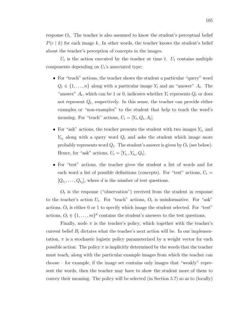
105
response Ot. The teacher is also assumed to know the student’s perceptual belief
P (c | k) for each image k. In other words, the teacher knows the student’s belief
about the teacher’s perception of concepts in the images.
Ut is the action executed by the teacher at time t. Ut contains multiple
components depending on Ut’s associated type:
• For “teach” actions, the teacher shows the student a particular “query” word
Qt ∈ {1, . . . , n} along with a particular image Yt and an “answer” At. The
“answer” At, which can be 1 or 0, indicates whether Yt represents Qt or does
not represent Qt, respectively. In this sense, the teacher can provide either
examples or “non-examples” to the student that help to teach the word’s
meaning. For “teach” actions, Ut = [Yt, Qt, At].
• For “ask” actions, the teacher presents the student with two images Yt1 and
Yt2 along with a query word Qt and asks the student which image more
probably represents wordQt. The student’s answer is given byOt (see below).
Hence, for “ask” actions, Ut = [Yt1 , Yt2 , Qt].
• For “test” actions, the teacher gives the student a list of words and for
each word a list of possible definitions (concepts). For “test” actions, Ut =
[Qt1 , . . . , Qtd ], where d is the number of test questions.
Ot is the response (“observation”) received from the student in response
to the teacher’s action Ut. For “teach” actions, Ot is uninformative. For “ask”
actions, Ot is either 0 or 1 to specify which image the student selected. For “test”
actions, Ot ∈ {1, . . . ,m}d contains the student’s answers to the test questions.
Finally, node π is the teacher’s policy, which together with the teacher’s
current belief Bt dictates what the teacher’s next action will be. In our implemen-
tation, π is a stochastic logistic policy parameterized by a weight vector for each
possible action. The policy π is implicitly determined by the words that the teacher
must teach, along with the particular example images from which the teacher can
choose – for example, if the image set contains only images that “weakly” repre-
sent the words, then the teacher may have to show the student more of them to
convey their meaning. The policy will be selected (in Section 5.7) so as to (locally)

106
minimize the expected cost of teaching, which we define as∑τ
t=1 γtc(ut) where
c(ut) is the expected amount of time, in seconds, necessary to execute action ut.
We assume that all actions of the same type (“teach”, “ask”, and “test”) take the
same amount of time and estimate these times from data of real students. We set
τ = 500 and γ = 1; hence, this is an undiscounted, finite-horizon control problem.
5.6.1 Representing and updating Bt
During the entire teaching session, the teacher must maintain and update a
probability distribution bt.= P (st | u1:t−1, o1:t−1) over the student’s state St. After
executing action Ut and receiving observation Ot from the student, the teacher
computes its new belief Bt+1 about the student’s new state St+1:
bt+1.= P (st+1 | u1:t, o1:t)
∝ P (st+1, ot | u1:t, o1:t−1)
=∑st
P (st+1, ot | st, u1:t, o1:t−1)P (st | u1:t, o1:t−1)
=∑st
P (st+1 | st, ut)P (ot | st, ut)P (st | u1:t−1, o1:t−1)
=∑st
P (st+1 | st, ut)P (ot | st, ut)bt
The first term in the summation represents the transition dynamics of the student’s
state, and the second term represents the observation likelihood model of the
student. These terms were both developed in Section 5.5. The third term in the
summation is the teacher’s prior belief bt.
Unfortunately, the student’s state contains Mt, which itself is a real-valued
matrix, and hence representing bt in exact form is infeasible. Instead, we use a
particle filter with importance resampling [40] to represent this distribution approx-
imately. This approach was previously applied to an automated teaching problem
in [71]. Each particle stores a possible student state st comprising the student’s
belief mt, values for αt and βt, and an absorption matrix vt. Associated with the
pth particle is a weight wp, such that the sum of the weights over all particles is
unity. We denote the student’s belief mt as represented by the pth particle as mpt.

107
αpt and βpt have analogous meanings. At each timestep, when the teacher exe-
cutes action ut and then receives an observation ot from the student, each particle
is updated according to the dynamics model in Section 5.5.3 and then reweighted
according to how well it explains ot according to the observation model in Section
5.5.4. The particle weights are then re-normalized to 1.
5.7 Computing a policy
Now that the teaching problem has been defined as a POMDP, we can
consider the various methods for solving it, i.e., for computing a policy π that
maps the teacher’s belief (more specifically, features of the teacher’s particles) at
time t into its next action. One simple approach to making decisions which works
with both finite and infinite (as in our case) state spaces is forward search; this was
the approach used to develop a math concept teacher in [71]. At timestep t, the
teacher considers every possible action ut it could take, and for each ut, it considers
every possible subsequent trajectory of subsequent states, actions, and observations
that might ensue for h timesteps (the planning horizon) into the future. The
teacher chooses action ut so as to minimize the expected cost, summed over h
timesteps, of executing action ut first. While simple to implement, this approach
is limited: Since the “tree” of possible trajectories grows exponentially in size with
the planning horizon h, and since this forward search must be conducted at run-
time when there are hard computational constraints (the teacher should not take
too long to decide its next action), h must typically be kept quite small (in [71], h
was 2). This leads to the concrete problem in our case that the teacher will never
decide to execute a “test” action because the immediate cost of testing is typically
an order of magnitude higher than the “teach” actions. Given a small planning
horizon h, it is always cheaper simply to execute h “teach” actions in succession
rather than execute one “test” action – hence, the student will never be given a
chance to graduate from the learning session.
Due to the small planning horizon issue, we instead chose a policy gradient
approach to optimizing the control policy, which requires a control policy that

108
can be expressed in some parametric form. Optimization of the policy parameters
can be performed offline when computational constraints are less pressing. In
addition, instead of exhaustively searching through a tree exponentially large in the
the planning horizon, policy gradient approaches sample many linear trajectories
of length τ , where τ is the time horizon of the POMDP itself. Hence, a policy
optimized with policy gradient can choose actions whose benefit might not be
realized until much further in the future. Nevertheless, even the policy gradient
approach we use does not completely solve the computational issues involved in
computing a policy. To simplify computation further, we employ a two-tiered
approach: In the first tier (“macro-controller”), we use a stochastic logistic policy
to decide, based on certain features of the teacher’s particles, whether to test,
teach word j, or ask a question about word j. This macro-controller does not
decide which image(s) to show for word j. The second tier (“micro-controller”),
given the decision to teach/ask about word j, decides which particular images
would be best based on an information-gain heuristic.
5.7.1 Macro-controller
We use a stochastic logistic policy that maps the teacher’s particles not into
a single action, but instead into a probability distribution over actions. We define
π(xt).= P (Ut = u | xt) ∝ exp(x>t wu)
where Ut is the action executed at time t, xt is a vector encoding certain features of
the teacher’s particles at time t, and wu is a weight vector associated with action
u ∈ U , where U is the action space of the macro-controller. We defined
U = {test, teach1, . . . , teachn, ask1, . . . , askn}
For simplicity, the “test” actions always asked the student about all n words; hence,
there is only one “test” action in U . Also, we restricted the “teach” actions to only
show positive examples for each word, i.e., Atqt is always 1.
We define xt to consist of the following features:

109
• For each word j, the expected (w.r.t. the teacher’s particles) “goodness”∑pwpg(mptj) of the student’s belief about word j, where goodness is defined
as
g(mtj).= mtji for i = Wj (5.10)
In other words, the goodness of the student’s belief about the meaning of
word j is the probability she assigns to the correct concept.
• The expected (w.r.t. the teacher’s particles) total uncertainty∑p
wp∑j
u(mptj)
over the student’s belief, summed over all words, where the uncertainty u is
defined as
u(mptj).= (mptj −mtj)
>(mptj −mtj)
and where
mtj.=∑p
wpmptj
In other words, u(mptj) expresses how far particle p’s opinion about Mt is
from the “mean belief” mpt. Note that the uncertainty is over the teacher’s
belief about the student’s belief; it is not over the student’s belief itself. (The
latter uncertainty is instead captured by the “goodness” defined above.)
• A bias term (constant 1).
To compute the policy weight vectors, we use the REINFORCE [98] policy
gradient technique. Since we have a model of the student, we can run simulations
to estimate the value and gradient of a particular policy as parameterized by
{wu}u∈U . Whenever the macro-controller decides either to teach or ask about
word j, it queries the micro-controller (see below) to determine the particular
image(s) it should present in conjunction with j. For each gradient estimate, we
ran 500 simulations of at most 500 timesteps (a simulation can end early if the
simulated student passes the test) using 100 particles. The learning rate was set
to 0.005, and the policy was optimized over 400 gradient descent steps.

110
At run-time, given the particles expressing the teacher’s belief bt, policy π
computes the probability over each action. The particular action chosen by the
teacher at that timestep is then sampled according to these probabilities.
5.7.2 Micro-controller
Given the decision at time t to teach (or ask about) word j, the teacher
needs a mechanism to select an image (or pair of images) for j. For the micro-
controller we use a 1-step lookahead search based on a information-maximization
heuristic. In particular, for the “teach” actions, the teacher selects image k so as
to maximize the expected (w.r.t. the particles) increase, from time t to t + 1, in
the goodness of the student’s belief about word j, where goodness is defined by
Equation 5.10 above.
For “ask” actions, the teacher chooses k1, k2 so as to maximize the expected
reduction in the teacher’s “total uncertainty” from time t to t+1. We define “total
uncertainty” as:∑p
wp∑j
u(mptj) +∑p
wp(αpt − αt)2 +∑p
wp(βpt − βt)2
where αt.=∑
pwpαpt and βt.=∑
pwpβpt. This metric includes uncertainty not
just over the student’s belief, but also over student parameters αt and βt.
5.8 Procedure to train automatic teacher
Given the models of the student and teacher, the particle-based belief up-
date mechanism, and the method of computing a teaching policy, we are now ready
to put all the parts together and create a prototype automated language teacher.
The procedure for creating a teacher of n words is the following:
1. Collect database of images Y = {1, . . . , l} with which to teach the words.
2. Query human subjects on which concepts they believe are represented by the
images, i.e., estimate P (c | k) for each image k ∈ Y .

111
Table 5.1: List of words and associated meanings taught during a word learningexperiment.
Word Meaningduzetuzi manfota womannokidono boymininami girlpipesu dogmekizo catxisaxepe birdbotazi rabbitkoto eatnotesabi drink
3. Collect data from human subjects to estimate the time costs (in seconds)
for “teach”, “ask”, and “test” actions, as well as student model parameters
P (α), P (β) by teaching students using an arbitrary teaching policy.
4. Execute gradient descent on policy parameters W to locally minimize the
expected teaching cost using the REINFORCE [98] policy gradient algorithm.
We implemented this procedure and tested the efficacy of the resulting teaching
policy; the experiment is described in the next section.
5.9 Experiment
We evaluated the procedure described in Section 5.8 using 10 words from
a synthetically generated foreign language with the associated meanings listed in
Table 5.1. The concept set consisted of all of the 10 meanings listed above plus
an additional “other” concept whose purpose was to account for everything that
subjects might perceive in the images that is not one of the words’ meanings.
Hence, there were n = 10 foreign words and m = 11 concepts in total.
We collected an image set of 56 images, each of which showed one of the
humans/animals in the concept set that was either eating or drinking. The images
are shown in Figure 5.5.

112
Figure 5.5: Image set used to teach foreign words that mean “man”, “cat”, “eat”,“drink”, etc. All images were found using Google Image Search.

113
We used a custom-built image labeling tool that asks the labeler to indicate,
for each image, “how strongly or weakly the image represents each of the listed
concepts” using a slider bar for each of the 11 concepts (including “other”). The
scale of each slider is from 0 to 1 and can thus be used as a reasonable estimate of
P (c | k) for each concept and image combination.
Next, we estimated the time costs and student model parameters from
42 subjects from the Amazon Mechanical Turk. The subjects for this parameter
estimation phase were taught with one of three possible teaching policies described
below: a RandomWordTeacher, a HandCraftedTeacher, and OptimizedTeacher.
(The parameters of the teachers during this data collection phase were set by
hand.) Based on these pilot subjects, we computed the average time costs to be
c(teach) = 10.74, c(ask) = 7.53, and c(test) = 106.46 seconds, respectively. For
simplicity, we assumed αt, βt were constant across the learning session (but possibly
different for each student).
Finally, we conducted policy gradient on the stochastic logistic policy’s
weight vectors using the costs and parameters estimated in the previous step. We
set the time horizon τ = 500 and the learning rate to 0.005. In practice, we
found that the choice for the learning rate was important – if it was too high,
then policy gradient descent sometimes converged to a nonsensical solution such
as never testing the student at all. We executed gradient descent for 400 iterations.
We call the resultant policy the OptimizedTeacher.
5.9.1 How the OptimizedTeacher behaves
The parameter set {wu}u∈U , concatenated row-wise into a matrix, is shown
in Figure 5.6. For a vocabulary of n = 10 words there are 21 rows – one “teach”
and “ask” action for each word, plus a “test” action. g(j) represents the goodness
of the student’s belief about word j as estimated by the teacher’s particles. At
run-time, each vector wu is multiplied (inner-product) by the feature vector xt
computed from the teacher’s particles, which in turn gives a scalar proportional to
the probability of executing action u under the policy. In the figure, dark colors
represent low weights, and light colors represent high weights. First, notice that

114
Teach 1Ask 1
Teach 2Ask 2
Teach 3Ask 3
Teach 4Ask 4
Teach 5Ask 5
Teach 6Ask 6
Teach 7Ask 7
Teach 8Ask 8
Teach 9Ask 9
Teach 10Ask 10
Test
G(1
)
G(2
)
G(3
)
G(4
)
G(5
)
G(6
)
G(7
)
G(8
)
G(9
)
G(1
0)
Unc
erta
inty
Bias
Figure 5.6: Policy of the OptimizedTeacher. Each row corresponds to the policyweight vector wu for the action specified on the left, e.g., “Teach j” means teachthe word indexed by j. Dark colors correspond to low values of the associatedweight vector; light colors represent high values.

115
the “bias” feature (last column) for the “test” action (last row) is very dark, i.e.,
has a very low weight – this means that the teacher tends not to execute “test”
actions very often. In addition, notice that the “uncertainty” feature for “test”
is also quite dark – the teacher does not like to test when it is uncertain about
the student’s beliefs. Finally, notice how the “goodness” features 1, . . . , 10 for the
“test” action are very light – if the teacher believes the student’s beliefs are good,
then this increases the probability that the teacher will “test”.
Next, observe the “staircase” effect along the diagonal – for every “teach”
action j, the teacher tends not to teach word j if the student’s belief for word j
is already good – this makes sense since teaching the student a word she already
knows would be a waste of time.
Finally, the “ask” actions tend to be executed rarely, as evidenced by the
dark color associated with most of their features. This is likely because the binary
questions that we constrained the teacher to ask provide relatively little informa-
tion, especially compared to a “test”, which contains d questions at once.
In order to measure the teaching effectiveness of the computed Optimized-
Teacher, we compared it to two other teaching strategies: a HandCraftedTeacher
and a RandomWordTeacher. The performance metric was the average amount of
time, in seconds, that a student would take to learn the words and pass the test.
5.9.2 RandomWordTeacher
We designed a teaching policy called the RandomWordTeacher that selects
a word uniformly at random from the vocabular {1, . . . , n} at each round. Then,
to teach word j, the RandomWordTeacher randomly selects an image k with prob-
ability proportional to P (c | k) where Wj = c. The RandomWordTeacher only
shows positive examples, i.e., Atqt is always 1. Every δ rounds, the Random-
WordTeacher gives a test to the student; if the student passes (accuracy at least
90% correct), then the teaching session is over. Otherwise, teaching continues for
another δ rounds, then the teacher gives another test, and so on. The maximum
length of the teaching session is τ = 500 rounds total (including tests). Parameter
δ ∈ {5, 10, . . . , 45, 50} was optimized in simulation and set to δ = 35.

116
Note that the RandomWordTeacher does not select an image to teach word
j uniformly at random – this would be almost nonsensical and could frequently
result in showing, for example, an image of a rabbit to teach that meaning of
the word fota equals “woman”. Instead, the RandomWordTeacher actually uses
part of the student model of the Optimized Teacher, namely the perceptual belief
P (c | k).
5.9.3 HandCraftedTeacher
The HandCraftedTeacher is a reasonable teaching policy that we crafted by
hand and which uses the student’s responses to the test questions to teach more
effectively. In other words, it is a closed-loop teacher.
The HandCraftedTeacher keeps track of how many times it has taught
each vocabulary word. At each round, it computes the set of words that have
been taught for fewer than ε = 3 times (parameter optimized in simulation) and
chooses one of those words uniformly at random. For the chosen word, the Hand-
CraftedTeacher then chooses an image with probability proportional to P (c | k)
where Wj = c. The HandCraftedTeacher only shows positive examples, i.e., Atqt
is always 1.
As soon as the HandCraftedTeacher has determined that each of the n
words has been taught ε times, it gives the student a test. If the student passes,
then the session is over; otherwise, the HandCraftedTeacher sets the counter of
every word that the student answered incorrectly on the test to 0. It then resumes
selecting a word that has been taught fewer than ε times. Note that this teaching
strategy was designed not to teach the same words needlessly when other words
have not been taught at all; it focuses the teaching on those words that the student
did not learn well based on test performance; and, like the RandomWordTeacher,
it capitalizes on the perceptual model P (c | k) to teach each word.

117
5.9.4 Experimental conditions
We constructed a simple teaching interface using Javascript and conducted
a study on 90 human subjects from the Amazon Mechanical Turk. Because we were
interested more in how the student learns the words’ meanings rather than how
well students can remembered them, we allowed students to use a “notepad” during
the learning session, implemented using a textbox within the teaching system.
In our experiment there were three experimental conditions to which sub-
jects were randomly assigned: OptimizedTeacher (N = 29), HandCraftedTeacher
(N = 35), and RandomWordTeacher (N = 26). Subjects were paid $0.15 for
completing the experiment, defined as passing the test (accuracy at least 90%).
Because the payment was fixed, subjects were economically motivated to learn as
efficiently as possible. In pilot experimentation, we found that offering a monetary
reward for faster learning (in addition to the base payment for participation) had
little effect on subjects’ performance.
5.9.5 Results
Results are shown in Figure 5.7. The OptimizedTeacher delivered the best
performance with an average time to learn the words and pass the test of 539.81
seconds; this was statistically significantly better (p < 0.01) than the Random-
WordTeacher condition, in which subjects took an average of 735.77 seconds – a
24% improvement. The OptimizedTeacher also performed slightly better than the
HandCraftedTeacher (mean time to completion of 560.99 seconds).
The results suggest that the procedure from Section 5.8 can produce an
automated teacher that performs equally well as a reasonable hand-crafted policy.
The advantage of the policy computation procedure proposed in this paper is that,
should the image statistics or time costs change, e.g., for a different vocabulary of
words, or for a different population of students, then the same procedure outlined
in Section 5.8 could be executed to automatically account for the change when
computing a new policy. In addition, having an explicit model of the student’s
beliefs is useful when creating an affect-sensitive teacher, as explored in Section
5.10. Finally, the performance of the OptimizedTeacher also lends support to

118
OptimizedTeacher HandCraftedTeacher RandomWordTeacher500
550
600
650
700
750
800
850
Avg
tim
e t
o f
inis
h (
sec)
Avg time to finish v. teaching strategy
Figure 5.7: Average time to completion of learning task versus experimentalcondition. Error bars show standard error of the mean of each group.
the paradigm of modeling the student as a Bayesian learner: even though human
students may not be perfect computers of Bayesian belief updates, the student
model was sufficiently accurate to teach students in a reasonable manner.
5.9.6 Correlation between time and information gain
Since the human subjects in the experiment were economically motivated
to complete the task quickly, it is possible that they themselves could compensate
for any poor teaching examples chosen by teachers. For example, if the student
already learned that the word pipesu means dog, and yet the automated teacher
chose to show him/her even more examples to convey pipesu’s meaning, then
perhaps the student would simply “click through” that example quickly to reach
more informative word+image combinations.
To test this hypothesis, we computed the average Pearson correlation over
all subjects between the time (in seconds) spent on each round in which the teacher
executed a “teach” action, and the expected increase in belief “goodness” (Equa-
tion 5.10) given the chosen image+word combination, by the student during that
round. The average correlation, which was statistically significant (p < 0.01), was
r = 0.28. This suggests that the students’ own behavior may have moderated the

119
influence of the particular teaching strategy.
5.10 Incorporating affect
A key challenge for the ITS community today is to design mechanisms to
incorporate “affective” observations of the student, such as those captured by a web
camera, into the decision-making process. POMDPs are a natural framework for
using affective sensor inputs, and here we propose and demonstrate in simulation
a simple architecture for how this might be done.
Consider a learning setting in which the student goes through phases in
which she is “trying” or “not trying”. When the student is trying, she processes
each image+word combination fully, i.e., her belief update strength βt is high.
When asked a question about a word+image pair or on a test, she tries to answer
correctly and answers according to her beliefs. In contrast, when a student is not
trying, her belief update strength and answer discriminability are low.
As a teacher, it is important to know when the student is receptive to
learning. It is also important to attribute mistakes on a test, or incorrect answers
to posed questions, to the proper cause: did the student really not know the
correct answer, or was she simply not trying? In other words, it is valuable, in this
example, for the teacher to have a good estimate of βt.
Note that the teacher already has some ability to estimate βt through the
student’s responses to questions and tests. If the student previously answered
several questions about the same word correctly, and yet now she answers them
incorrectly, then this is probably because she has stopped trying. However, ques-
tions and tests will likely be issued relatively rarely due to their cost; hence, the
teacher’s estimate of βt may be very uncertain.
Now, suppose the teacher has access to some kind of “affective sensor”,
e.g., an estimate of how hard the student is trying as measured by a classifier
that processes images captured by a web camera. These sensor inputs could be
used to estimate βt much more precisely. If the teacher also had some mechanism
with which to re-“engage” the student in the task, and if the teacher executed this

120
action judiciously, then it could potentially teach more effectively.
5.10.1 Simulation
To illustrate the potential utility of incorporating affective state estimates
into the decision-making process, we conducted a simulation, using the same words
and image statistics from Section 5.9, comparing two automated teachers that
teaches students who can “stop trying” as described above. In particular, we let
βt ∈ {0.25, 0.95} for each t, and we suppose that over time the student tends
to stop trying, i.e., with probability 0.05, she will transition from βt = 0.95 to
βt+1 = 0.25. In order to help the teacher teach more effectively, we endow both
teachers with an additional “engage” action, which causes the student to enter
the “trying” state (βt+1 = 0.95) with some probability 1. However, the “engage”
action also incurs a cost – we suppose that it is 4 times more expensive than a
“teach” action. In order to encourage the “engage” action to be selected when βt
was estimated by the teacher to be low, we added an added an extra element to the
feature vector xt of the particles, namely the expected value (w.r.t. the teacher’s
particles) of βt:∑
pwpβpt.
We compare one teacher with “affective sensors” to another teacher that
does not have affective sensors. The teacher with affective sensors receives at every
timestep t an “affective observation” zt (in addition to the standard observation
ot) that depends only on βt. Here, we model zt as being generated from βt plus
some Gaussian noise:
P (zt | mt, αt, βt, vt).= N (µ = βt;σ
2 = 0.252)
where N is the normal distribution. At every timestep, the affective teacher up-
dates its belief about the student’s state at time t+ 1 (see Section 5.6.1) based not

121
just on ot, but now also on zt:
bt+1.= P (st+1 | u1:t, o1:t, z1:t)
∝ P (st+1, ot, zt | u1:t, o1:t−1, z1:t−1)
=∑st
P (st+1, ot, zt | st, u1:t, o1:t−1, z1:t−1)P (st | u1:t, o1:t−1, z1:t−1)
=∑st
P (st+1 | st, ut)P (ot, zt | st, ut)P (st | u1:t−1, o1:t−1, z1:t−1)
=∑st
P (st+1 | st, ut)P (ot | st, ut)P (zt | st, ut)bt
=∑st
P (st+1 | st, ut)P (ot | st, ut)P (zt | βt)bt
The value of the affective sensors can thus be defined by this additional term
P (zt | βt) which helps to (greatly) constrain the possible states st that could
explain the data observed by the teacher.
We used policy gradient descent (as before) to optimize the policies of both
the teacher with affective sensors and the teacher without them. The policies learnt
for both teachers in this simulation were similar to the policy shown in Figure 5.6.
For the “engage” action, the weight on the feature expressing the expected βt is
strongly negative, so that the teacher tends to execute “engage” when the teacher
believes that βt is low (i.e., student has stopped trying). In addition, the weight
for the “test” action associated with βt is also strongly negative, which encodes
the fact that asking a student to take a test when she is not trying is probably a
bad idea. These trends apply to the policies of both teachers – one with affective
sensors, one without. The key difference between them is that the teacher with
extra sensors can estimate βt more accurately than the other teacher.
In simulation, the utility of the benefit of having affective sensors, as mea-
sured by the student’s learning gains as a function of time, is displayed in Figure
5.8 (left). Results were averaged over 1000 simulation runs. The shaded area for
each teacher represent the teacher’s belief of the student’s belief goodness, summed
over all words, plus or minus one standard deviation for each timestep t. Notice
how the mean teacher’s belief of the student’s belief goodness is not only higher
for the teacher with affective sensors, but its uncertainty is also lower. Figure 5.8

122
0 50 100 150 2000
0.1
0.2
0.3
0.4
0.5
0.6
0.7
0.8
0.9
1
Timestep (t)
Pro
p.
of
stu
de
nts
wh
o p
as
se
d t
est
Without affective sensorsWith affective sensors
Figure 5.8: Simulation results comparing a teacher with “affective sensors” toone without them. The affect-sensitive teacher is able to teach the student morequickly (left), allowing the student to pass the test, on average, more quickly(right).
(right) shows the average amount of time for a student to pass the test for each
teacher. In agreement with the other graph, the teacher with affective sensors
helps its students to graduate more quickly on average. Finally, the average cost
of the teaching session (until either τ = 200 or the student passes the test) was
also lower for the teacher with affective sensors: 89.50sec for the affect-sensitive
teacher versus 133.25sec for the teacher without the extra sensors.
5.11 Summary
We have developed an automated foreign language teacher that teaches
words by image association, i.e., in the manner of Rosetta Stone language software
[73]. The student in this learning setting was modeled as a Bayesian learner;
the teaching problem was modeled as a POMDP; and the system’s controller was
optimized using a hierarchical policy gradient descent approach over features of
the teacher’s belief as represented by a particle filter. Results on a human subjects
experiment indicate that the policy computed using the proposed procedure can
deliver policies that perform favorably compared to reasonable baseline controllers.

123
Finally, we illustrate how the developed prototype teacher could be extended to
incorporate affective observations of the student, e.g., from a webcam, in order to
teach even more effectively.
5.12 Appendix: Conditional independence proofs
Below we prove two conditional independence theorems about the random
variables shown in the graphical model of Figure 5.2.
5.12.1 d-Separation of Wj from Wj′ for j′ 6= j
We show that
P (w1, . . . , wn | y1:t, a1q1 , . . . , atqt) =∏j
P (wj | y1:t, a1q1 , . . . , atqt)
All we must show is that Wj is conditionally independent of Wj′ given Y1:t and
A1q1 , . . . , Atqt for all j′ 6= j. To prove this conditional independence we will use
graph theory and show that every undirected path between Wj and Wj′ is d-
separated. (For brevity, we will omit the word “undirected”.) First, note that it
suffices to show that every path without cycles betwen Wj and Wj′ is d-separated:
any path with cycles can be trivially converted to a path without cycles, and if
the simplified path (with no cycles) is d-separated, then so too will be the original
path.
Our proof proceeds in two parts. In Part 1, we will show that any path P
from Wj to Wj′ must contain two nodes Aνj and Aνj′ for some timestep ν such that
j′ 6= j. In Part 2 we will use the fact that, at every round ν, the student observes
at most one node Aνj to show that the other, unobserved node Aνj′ d-separates
Wj from Wj′ .
Part 1: Notice that the only nodes to which Wj is connected are
A1j, . . . , Atj; hence P must start with the nodes WjAνj for some ν. Now, consider
the next node in P after Aνj: the only nodes to which Aνj is connected are Cν
and Wj. We can ignore the latter possibility because a path that starts out as
WjAνjWj would contain a cycle. Hence, P must start out as WjAνjCν . From the

124
graphical model it is clear that any path from Cν to Wj′ must eventually proceed
through some node Aνj′ . The only remaining question is whether j′ = j or j′ 6= j.
However, we can discard the former possibility because that would result in a cycle.
Hence, every path P from Wj to Wj′ must contain two nodes Aνj and Aνj′ such
that j′ 6= j for some timestep ν.
Part 2: To finally prove d-separation between Wj and Wj′ , we note that,
at each timestep ν, at most one of Aνj and Aνj′ can be observed by the student
because only one query is “answered” at each timestep. Since at least one of those
two nodes is unobserved, and since none of the A nodes has any descendants, then
P is d-separated (by the “inverted fork” rule) by either Aνj or Aνj′ . Since this is
true of any path P without cycles, we conclude that Wj is d-separated from Wj′ .
5.12.2 d-Separation of Wj from Aνqν for all ν such that qν 6= j
We prove that
P (wj | y1:t, a1q1 , . . . , atqt) = P (wj | y1:t, {aνj}ν:qν=j)
In other words, belief about Wj is not affected by answers to queries about other
words j′ 6= j. Consider any timestep ν for which qν 6= j, and consider any path P
from Aνqν to Wj. In order for P to reach Wj, it must pass through either Wqν or
through Aνj. In the former case, we already know (from Appendix 5.12.1, where
the set of observed nodes was the same) that every path P ′ from Wj to Wj′ is
d-separated for all j′ 6= j; hence, path P would also be d-separated. In the latter
case, since Aνqν is observed, and since at most one A node is observed at any one
timestep, then node Aνj cannot be observed; hence, Aνj d-separates Aνqν from Wj.
In either case, Wj is d-separated from Aνqν for any ν such that qν 6= j. Hence, Wj
is conditionally independent of Aνqν for any ν such that qν 6= j:
5.13 Acknowledgement
Chapter 5, in full, is currently being prepared for submission for publication
of the material. Jacob Whitehill and Javier Movellan. The dissertation author was

125
the primary investigator and author of this material.
Bibliography
[1] G. Aist, B. Kort, R. Reilly, J. Mostow, and R. Picard. Experimentallyaugmenting an intelligent tutoring system with human-supplied capabilities:adding human-provided emotional scaffolding to an automated reading tutorthat listens. In Proc. Multimodal Interfaces, 2002.
[2] V. Aleven and K. Koedinger. Limitations of student control: Do studentsknow when they need help? In Intelligent Tutoring Systems: 5th Interna-tional Conference, 2000.
[3] J. R. Anderson. The Architecture of Cognition. Harvard University Press,1983.
[4] J. R. Anderson. Rules of the Mind. Lawrence Erlbaum Associates, 1993.
[5] J. R. Anderson, C. F. Boyle, and B. J. Reiser. Intelligent tutoring systems.Science, 228(4698):456–462, 1985.
[6] R. C. Atkinson. Ingredients for a theory of instruction. Technical report,Stanford Institute for Mathematical Studies in the Social Sciences, 1972.
[7] R. C. Atkinson. Human Memory and the Learning Process: Selected Papersof Richard C. Atkinson, chapter Adaptive instructional systems: Some at-tempts to optimize the learning process. Progress Publishing House, Moscow,1980.
[8] Barnes and J. Stamper. Toward automatic hint generation for logic prooftutoring using historical student data. In Intelligent Tutoring Systems, 2008.
[9] M. Bartlett, G. Littlewort, M. Frank, C. Lainscsek, I. Fasel, and J. Movellan.Automatic recognition of facial actions in spontaneous expressions. Journalof Multimedia, 2006.
[10] M. Bartlett, G. Littlewort, M. Frank, C. Lainscsek, I. Fasel, and J. Movellan.Automatic recognition of facial actions in spontaneous expressions. Journalof Multimedia, 2006.
[11] M. Bartlett, G. Littlewort, M. Frank, C. Lainscsek, I. Fasel, and J. Movel-lan. Fully automatic facial action recognition in spontaneous behavior. InProceedings of the IEEE Conference on Automatic Facial and Gesture Recog-nition, 2006.
126

127
[12] J. Beck. Engagement tracing: using response times to model student disen-gagement. In Proceedings of the 2005 conference on Artificial Intelligence inEducation, 2005.
[13] J. Beck, K. Chang, J. Mostow, and A. Corbett. Does help help? introducingthe bayesian evaluation and assessment methodology. In Intelligent TutoringSystems, 2008.
[14] G. H. Bower. Application of a model to paired-associate learning. Psychome-trika, 26(3), 1961.
[15] N. J. Butko and J. R. Movellan. I-POMDP: An infomax model of eye-movement. In Proceedings of the International Conference on Developmentand Learning, 2008.
[16] I. Carnegie Learning. Carnegie learning, 2012.http://www.carnegielearning.com.
[17] A. R. Cassandra. The POMDP page, 2005.http://www.cassandra.org/pomdp/tutorial/index.shtml.
[18] M. Chaouachi, P. Chalfoun, I. Jraidi, and C. Frasson. Affect and mentalengagement: towards adaptability for intelligent systems. In FLAIRS, 2010.
[19] M. Chi, K. VanLehn, and D. Litman. Do micro-level tutorial decisions mat-ter: Applying reinforcement learning to induce pedagogical tutorial tactics.In Intelligent Tutoring Systems, 2010.
[20] C. Conati, A. Gertner, and K. VanLehn. Using bayesian networks to manageuncertainty in student modeling. User Modeling and User-Adapted Interac-tion, 12(4):371–417, 2004.
[21] A. T. Corbett and J. R. Anderson. Student modeling and mastery learn-ing in a computer-based programming tutor. In Proceedings of the SecondInternational Conference on Intelligent Tutoring Systems, 1992.
[22] A. Corporation. ALEKS, 2012. http://www.aleks.com.
[23] A. B. Craig. How do you feel – now? the anterior insula and human aware-ness. Nature reviews neuroscience, 10:59–70, 2009.
[24] derek T. Green, T. J. Walsh, P. R. Cohen, C. R. Beal, and Y.-H. Chang.gender differences and the value of choice in intelligent tutoring systems. Inconference on User Modeling, Adaptation, and Personalization, pages 341–346, 2011.
[25] S. D’Mello, B. Lehman, J. Sullins, R. Daigle, R. Combs, K. Vogt, L. Perkins,and A. Graesser. A time for emoting: When affect-sensitivity is and isn’teffective at promoting deep learning. In Intelligent tutoring systems, 2010.
[26] S. D’Mello, R. Picard, and A. Graesser. Towards an affect-sensitive auto-tutor. IEEE Intelligent Systems, Special issue on Intelligent EducationalSystems, 22(4), 2007.

128
[27] S. D’Mello, R. Picard, and A. Graesser. Towards an affect-sensitive auto-tutor. IEEE Intelligent Systems, Special issue on Intelligent EducationalSystems, 22(4), 2007.
[28] S. K. D’Mello, S. Craig, J. Sullins, and A. Graesser. Predicting affectivestates expressed through an emote-aloud procedure from autotutors mixe-dinitiative dialogue. International Journal of Artificial Intelligence in Edu-cation, 2005.
[29] T. Dragon, I. Arroyo, B. Woolf, W. Burleson, R. el Kaliouby, and H. Ey-dgahi. Viewing student affect and learning through classroom observationand physical sensors. In Intelligent tutoring systems, 2008.
[30] Duolingo. duolingo.com, 2012.
[31] P. Ekman. Emotion in the Human Face. Cambridge University Press, NewYork, 2 edition, 1982.
[32] P. Ekman and W. Friesen. The Facial Action Coding System: A TechniqueFor The Measurement of Facial Movement. Consulting Psychologists Press,Inc., San Francisco, CA, 1978.
[33] S. Fairclough and L. Venables. Prediction of subjective states from psy-chophysiology: a multivariate approach. Biological psychology, 71:100–110,2006.
[34] I. Fenwick and M. D. Rice. Reliability of continuous measurement copy-testing methods. Journal of Advertising Research, 1991.
[35] D. Fossati, B. D. Eugenio, S. Ohlsson, C. Brown, L. Chen, and D. Cosejo. Ilearn from you, you learn from me: How to make ilist learn from students.In The 14th International Conference on Artificial Intelligence in Education,2009.
[36] Y. Freund and R. E. Schapire. A decision-theoretic generalization of on-line learning and an application to boosting. In European Conference onComputational Learning Theory, pages 23–37, 1995.
[37] J. Friedman, T. Hastie, and R. Tibshirani. Additive logistic regression: astatistical view of boosting. Annals of Statistics, 28(2), 2000.
[38] H. Gamboa and A. Fred. Designing intelligent tutoring systems: a bayesianapproach. In Proceedings of the Ana Fred 3rd International Conference onEnterprise Information Systems, 2001.
[39] B. Goldberg, R. Sottilare, K. Brawner, and H. Holden. Predicting learnerengagement during well-defined and ill-defined computer-based interculturalinteractions. In Proceedings of the 4th international conference on Affectivecomputing and intelligent interaction, 2011.
[40] N. Gordon, D. Salmond, and A. Smith. Novel approach to nonlinear/non-gaussian bayesian state estimation. IEE Proceedings F, Radar and SignalProcessing, 140:107–13, 1993.

129
[41] B. Guerin. Mere presence effects in humans: A review. Journal of Experi-mental Social Psychology, 1986.
[42] O. Hill, Z. Serpell, and J. Turner. Transfer of cognitive skills training tomathematics performance in minority students. In Poster at annual meetingof Association for Psychological Sciences, Boston, MA, 2010.
[43] M. Holland and G. Tarlow. Blinking and mental load. Psychological Reports,31(1), 1972.
[44] M. Hoque and R. Picard. Acted vs. natural frustration and delight: Manypeople smile in natural frustration. In Proc. Automatic Face and GestureRecognition (FG’11), 2011.
[45] S. Jaeggi, M. Buschkuehl, J. Jonides, and W. Perrig. Improving fluid in-telligence with training on working memory. Proceedings of the NationalAcademy of Sciences, 2008.
[46] J. Johns and B. Woolf. A dynamic mixture model to detect student motiva-tion and prociency. In AAAI, 2006.
[47] A. Kapoor, W. Burleson, and R. Picard. Automatic prediction of frustration.International Journal of Human-Computer Studies, 65(8), 2007.
[48] A. Kapoor, S. Mota, and R. Picard. Towards a learning companion thatrecognizes affect. In AAAI Fall Symposium, 2001.
[49] K. R. Koedinger and J. R. Anderson. Intelligent tutoring goes to school inthe big city. International Journal of Artificial Intelligence in Education,8:30–43, 1997.
[50] S. Koelstra, M. Pantic, and I. Patras. A dynamic texture based approachto recognition of facial actions and their temporal models. Pattern Analysisand Machine Intelligence, 2010.
[51] I. Kotsia and I. Pitas. Facial expression recognition in image sequencesusing geometric deformation features and support vector machines. IEEETransactions on Image Processing, 16(1), 2007.
[52] M. Lades, J. C. Vorbruggen, J. Buhmann, J. Lange, C. von der Malsburg,R. P. Wurtz, and W. Konen. Distortion invariant object recognition in thedynamic link architecture. IEEE Transactions on Computers, 42:300–311,1993.
[53] J. H. Laubsch. A adaptive teaching system for optimal item allocation.Technical report, Stanford Institute for Mathematical Studies in the SocialSciences, 1969.
[54] LearningRx. LearningRx, 2012. www.learningrx.com.
[55] G. Littlewort, M. Bartlett, I. Fasel, J. Susskind, and J. Movellan. Dynamicsof facial expression extracted automatically from video. Image and VisionComputing, 24(6), 2006.

130
[56] G. Littlewort, M. Bartlett, and K. Lee. Automatic coding of facial expres-sions displayed during posed and genuine pain. Image and Vision Computing,27(12):1797–1803, 2009.
[57] G. Littlewort, J. Whitehill, T. Wu, I. Fasel, M. Frank, J. Movellan, andM. Bartlett. Computer expression recognition toolbox. In Proc. AutomaticFace and Gesture Recognition (FG’11), 2011.
[58] S. Lucey, I. Matthews, C. Hu, Z. Ambadar, F. de la Torre, and J. Cohn. AAMderived face representations for robust facial action recognition. In Proc.IEEE International Conference on Automatic Face and Gesture Recognition,pages 155–160, 2006.
[59] S. Makeig, M. Westerfield, J. Townsend, T.-P. Jung, E. Courchesne, andT. J. Sejnowski. Functionally independent components of early event-relatedpotentials in a visual spatial attention task. Philosophical Transactions ofthe Royal Society: Biological Science, 354:1135–44, 1999.
[60] R. Marachi. Statistical analysis of cognitive change with Learning Rx trainingprocedures. Technical report, Department of Child and Adolescent Develop-ment, CSU Northridge, 2006.
[61] J. E. Matheson. Optimum teaching procedures derived from mathematicallearning models. Institute in Engineering-Economic Systems, Stanford Uni-versity, 1964.
[62] G. Matthews, S. Campbell, S. Falconer, L. Joyner, J. Huggins, andK. Gilliland. Fundamental dimensions of subjective state in performancesettings: task engagement, distress, and worry. Emotion, 2(4):315–340, 2002.
[63] B. McDaniel, S. D’Mello, B. King, P. Chipman, K. Tapp, and A. Graesser.Facial features for affective state detection in learning environments. InProceedings of the 29th Annual Cognitive Science Society, 2007.
[64] J. Movellan, F. Tanaka, I. Fasel, C. Taylor, P. Ruvolo, and M. Eckhardt.The rubi project: a progress report. In Proceedings of the ACM/IEEE In-ternational Conference on Human-Robot Interaction, pages 333–339, 2007.
[65] J. R. Movellan. Tutorial on gabor filters. Technical report, MPLab Tutorials,UCSD MPLab, 2005.
[66] R. C. Murray, K. VanLehn, and J. Mostow. Looking ahead to select tutorialactions: A decision-theoretic approach. International Journal of ArtificialIntelligence in Education, 2004.
[67] J. Nelson and G. Cottrell. A probabilistic model of eye movements in conceptformation. Neurocomputing, 70:2256–2272, 2007.
[68] J. Nelson and J. Movellan. Active inference in concept learning. In NIPS,2001.
131
[69] M. Pantic and J. Rothkrantz. Facial action recognition for facial expressionanalysis from static face images. IEEE Transactions on Systems, Man andCybernetics, 34(3), 2004.
[70] A. Pope, E. Bogart, and D. Bartolome. Biocybernetic system evaluatesindices of operator engagement in automated task. Biological psychology,40:187–195, 1995.
[71] A. Rafferty, E. Brunskill, T. Griffiths, and P. Shafto. Faster teaching byPOMDP planning. In Artificial intelligence in education, 2011.
[72] H. Rio, A. Soli, E. Aguirr, L. Guerrer, and J. A. Santa. Facial expressionrecognition and modeling for virtual intelligent tutoring systems. In Pro-ceedings of the Mexican International Conference on Artificial Intelligence:Advances in Artificial Intelligence, 2000.
[73] Rosetta Stone. www.rosettastone.com, 2012.
[74] N. Roy, G. Gordon, and S. Thrun. Finding approximate POMDP solutionsthrough belief compression. Journal of Artificial Intelligence Research, 23:1–40, 2005.
[75] J. Sanghvi, G. Castellano, I. Leite, A. Pereira, P. McOwan, and A. Paiva.Automatic analysis of affective postures and body motion to detect engage-ment with a game companion. In Human Robot Interaction, 2011.
[76] A. Sarrafzadeh, S. Alexander, F. Dadgostar, C. Fan, and A. Bigdeli. See me,teach me: Facial expression and gesture recognition for intelligent tutoringsystems. In Innovations in Information Technology, 2006.
[77] Scientific Learning. Scientific Learning, 2012. www.scilearn.com.
[78] P. Shafto and N. Goodman. Teaching games: Statistical sampling assump-tions for learning in pedagogical situations. In Proceedings of the ThirtiethAnnual Conference of the Cognitive Science Society, 2008.
[79] B. Skinner. Teaching machines. Science, 128(3330):969–977, 1958.
[80] R. Smallwood and E. Sondik. The optimal control of partially observablemarkov processes over a finite horizon. Operations Research, 21(5), 1971.
[81] R. D. Smallwood. The analysis of economic teaching strategies for a simplelearning model. Journal of Mathematical Psychology, 8:285–301, 1971.
[82] T. Smith. Zmdp software for pomdp and mdp planning, 2009.http://www.cs.cmu.edu/ trey/zmdp.
[83] M. T. Spaan and N. Vlassis. Perseus: Randomized point-based value iter-ation for POMDPs. Journal of Artificial Intelligence Research, 24:195–220,2005.
[84] P. Suppes. Problems of optimization in learning a list of simple items. InM. W. S. II and G. L. Bryan, editors, Human Judgments and Optimality.John Wiley and Sons, 1964.

132
[85] H. Tada. Eyeblink rates as a function of the interest valueof video stimuli.Tohoku Psychologica Folica, 45, 1986.
[86] J. Tenenbaum. Bayesian modeling of human concept learning. In Advancesin Neural Information Processing Systems, 1999.
[87] Y. Tian, T. Kanade, and J. Cohn. Recognizing action units for facial expres-sion analysis. IEEE Transactions on Pattern Analysis and Machine Intelli-gence, 23(2), 2001.
[88] Y. Tong, W. Liao, and Q. Ji. Facial action unit recognition by exploitingtheir dynamic and semantic relationships. IEEE Transactions on PatternAnalysis and Machine Intelligence, 29(10):1683–1699, 2007.
[89] K. VanLehn. The interaction plateau: Answer-based tutoring < stepbasedtutoring = natural tutoring. In Keynote address of the Intelligent TutoringSystems conference, 2008.
[90] K. VanLehn, C. Lynch, K. Schultz, J. Shapiro, R. Shelby, and L. Taylor.The andes physics tutoring system: Lessons learned. International Journalof Artificial Intelligence and Education, 15(3):147–204, 2005.
[91] R. Vesselinov. Measuring the effectiveness of rosetta stone. Technical report,Queens College, City University of New York, 2009.
[92] P. Viola and M. Jones. Robust real-time object detection. InternationalJournal of Computer Vision, 2004.
[93] E. Vural, M. Cetin, A. Ercil, G. Littlewort, M. Bartlett, and J. Movel-lan. Drowsy driver detection through facial movement analysis. In Human-Computer Interaction, 2007.
[94] J. Whitehill, M. Bartlett, and J. R. Movellan. Automatic facial expressionrecognition for intelligent tutoring systems. In Proceedings of the CVPR 2008Workshop on Human Communicative Behavior Analysis, 2008.
[95] J. Whitehill, G. Littlewort, I. Fasel, M. Bartlett, and J. Movellan. Towardpractical smile detection. Pattern Analysis and Machine Intelligence, 2009.
[96] J. Whitehill and J. Movellan. A discriminative approach to frame-by-framehead pose tracking. In Proc. Automatic Face and Gesture Recognition(FG’08), 2008.
[97] J. Whitehill, Z. Serpell, A. Foster, Y.-C. Lin, B. Pearson, M. Bartlett, andJ. Movellan. Towards an optimal affect-sensitive instructional system ofcognitive skills. In Computer Vision and Pattern Recognition Workshop onHuman Communicative Behavior, 2011.
[98] R. J. Williams. Simple statistical gradient-following algorithms for connec-tionist reinforcement learning. Machine learning, 1992.
[99] B. Woolf, W. Burleson, I. Arroyo, T. Dragon, D. Cooper, and R. Picard.Affect-aware tutors: recognising and responding to student affect. Interna-tional Journal of Learning Technology, 4(3):129–164, 2009.

133
[100] T. Wu, N. Butko, P. Ruvolo, J. Whitehill, M. Bartlett, and J. Movellan.Multilayer architectures for facial action unit recognition. IEEE Transactionson Systems, Man, and Cybernetics B: Cybernetics, 2012.
[101] F. Xu and J. Tenenbaum. Word learning as bayesian inference. PsychologicalReview, 2007.
[102] P. Yang, Q. Liu, and D. N. Metaxas. Boosting encoded dynamic features forfacial expression recognition. Pattern Recognition Letters, 30:132–139, 2009.
[103] Z. Zhu and Q. Ji. Robust real-time face pose and facial expression recovery.In Computer Vision and Pattern Recognition, 2006 IEEE Computer SocietyConference on, 2006.