a stochastic evaluation of solvency …angus/papers/thesis.pdf · 4.1.1 timing of cash-°ows in the...
TRANSCRIPT

A STOCHASTIC EVALUATION OF SOLVENCY
VALUATIONS FOR LIFE OFFICES
By
Angus S. Macdonald
Submitted for the Degree of
Doctor of Philosophy
at Heriot-Watt University
on Completion of Research in the
Department of Actuarial Mathematics & Statistics
November 2004.
This copy of the thesis has been supplied on the condition that anyone who consults
it is understood to recognise that the copyright rests with its author and that no quo-
tation from the thesis and no information derived from it may be published without
the prior written consent of the author or the university (as may be appropriate).

I hereby declare that the work presented in this the-
sis was carried out by myself at Heriot-Watt University,
Edinburgh, except where due acknowledgement is made,
and has not been submitted for any other degree.
Angus S. Macdonald (Candidate)
Prof. A. D. Wilkie (Supervisor)
Date
ii

Contents
Acknowledgements xviii
Abstract xix
Introduction 10.1 Life office solvency . . . . . . . . . . . . . . . . . . . . . . . . . . . . 10.2 The traditional model . . . . . . . . . . . . . . . . . . . . . . . . . . 20.3 Stochastic approaches to solvency . . . . . . . . . . . . . . . . . . . . 30.4 Plan of this thesis . . . . . . . . . . . . . . . . . . . . . . . . . . . . . 5
0.4.1 Survey of some previous work . . . . . . . . . . . . . . . . . . 50.4.2 Introduction of a simple model . . . . . . . . . . . . . . . . . 50.4.3 Investment strategies . . . . . . . . . . . . . . . . . . . . . . . 50.4.4 Maturity value smoothing . . . . . . . . . . . . . . . . . . . . 50.4.5 Evaluating the traditional valuation model . . . . . . . . . . . 5
1 Background to U.K. life assurance 71.1 Investment and bonus policy since 1945 . . . . . . . . . . . . . . . . . 71.2 Asset shares . . . . . . . . . . . . . . . . . . . . . . . . . . . . . . . . 101.3 Discretion versus expectations . . . . . . . . . . . . . . . . . . . . . . 111.4 Other developments . . . . . . . . . . . . . . . . . . . . . . . . . . . . 13
1.4.1 Statutory minimum solvency . . . . . . . . . . . . . . . . . . . 131.4.2 E.C. solvency margins . . . . . . . . . . . . . . . . . . . . . . 141.4.3 The resilience test . . . . . . . . . . . . . . . . . . . . . . . . . 14
2 The traditional valuation model 152.1 Introduction . . . . . . . . . . . . . . . . . . . . . . . . . . . . . . . . 152.2 Redington’s 1952 paper . . . . . . . . . . . . . . . . . . . . . . . . . . 172.3 Skerman’s principles . . . . . . . . . . . . . . . . . . . . . . . . . . . 18
2.3.1 The 5th principle . . . . . . . . . . . . . . . . . . . . . . . . . 192.3.2 Other points made by Skerman . . . . . . . . . . . . . . . . . 202.3.3 Ammeter’s comments . . . . . . . . . . . . . . . . . . . . . . . 212.3.4 The adoption of the principles . . . . . . . . . . . . . . . . . . 22
2.4 The U.K. minimum solvency valuation basis . . . . . . . . . . . . . . 222.4.1 Valuation of assets . . . . . . . . . . . . . . . . . . . . . . . . 222.4.2 Valuation of liabilities . . . . . . . . . . . . . . . . . . . . . . 232.4.3 Consequences of Regulation 59 . . . . . . . . . . . . . . . . . 242.4.4 The 1994 Regulations . . . . . . . . . . . . . . . . . . . . . . . 25
iii
2.5 The E.C. solvency margins . . . . . . . . . . . . . . . . . . . . . . . . 272.5.1 The Campagne Reports . . . . . . . . . . . . . . . . . . . . . 282.5.2 The Buol Report . . . . . . . . . . . . . . . . . . . . . . . . . 28
2.6 The U.K. resilience test . . . . . . . . . . . . . . . . . . . . . . . . . . 292.6.1 The Government Actuary’s memorandum of 13 November 1985 292.6.2 The Government Actuary’s memorandum of 31 July 1992 . . . 312.6.3 The Government Actuary’s memorandum of 30 September 1993 33
2.7 North American and Australian developments . . . . . . . . . . . . . 342.7.1 The U.S.A . . . . . . . . . . . . . . . . . . . . . . . . . . . . . 352.7.2 Canada . . . . . . . . . . . . . . . . . . . . . . . . . . . . . . 402.7.3 The Australian valuation proposals . . . . . . . . . . . . . . . 42
3 Stochastic solvency studies 443.1 Introduction . . . . . . . . . . . . . . . . . . . . . . . . . . . . . . . . 443.2 The Wilkie asset model . . . . . . . . . . . . . . . . . . . . . . . . . . 463.3 The Maturity Guarantees Working Party . . . . . . . . . . . . . . . . 473.4 The Faculty Solvency Working Party . . . . . . . . . . . . . . . . . . 483.5 The Faculty Bonus and Valuation Research Group . . . . . . . . . . . 523.6 M. D. Ross . . . . . . . . . . . . . . . . . . . . . . . . . . . . . . . . 553.7 M. D. Ross & M. R. McWhirter . . . . . . . . . . . . . . . . . . . . . 603.8 The Finnish Solvency Working Group . . . . . . . . . . . . . . . . . . 653.9 Conclusions . . . . . . . . . . . . . . . . . . . . . . . . . . . . . . . . 68
4 A simple model office 704.1 Introduction . . . . . . . . . . . . . . . . . . . . . . . . . . . . . . . . 70
4.1.1 Timing of cash-flows in the model . . . . . . . . . . . . . . . . 714.1.2 Valuation of liabilities . . . . . . . . . . . . . . . . . . . . . . 714.1.3 Valuation of assets . . . . . . . . . . . . . . . . . . . . . . . . 724.1.4 Asset allocation rule . . . . . . . . . . . . . . . . . . . . . . . 734.1.5 Reversionary bonus rule . . . . . . . . . . . . . . . . . . . . . 734.1.6 Terminal bonus rule . . . . . . . . . . . . . . . . . . . . . . . 744.1.7 Premium rate . . . . . . . . . . . . . . . . . . . . . . . . . . . 744.1.8 Tax . . . . . . . . . . . . . . . . . . . . . . . . . . . . . . . . . 744.1.9 Expenses, lapses and mortality . . . . . . . . . . . . . . . . . 744.1.10 Generation of financial scenarios . . . . . . . . . . . . . . . . . 754.1.11 Starting point for the projections . . . . . . . . . . . . . . . . 75
4.2 Key financial ratios . . . . . . . . . . . . . . . . . . . . . . . . . . . . 754.2.1 The ratio A/L1 . . . . . . . . . . . . . . . . . . . . . . . . . . 754.2.2 The ratio A/L2 . . . . . . . . . . . . . . . . . . . . . . . . . . 764.2.3 The ratio A/AS . . . . . . . . . . . . . . . . . . . . . . . . . . 76
4.3 Some results using the basic model . . . . . . . . . . . . . . . . . . . 764.3.1 Financial conditions . . . . . . . . . . . . . . . . . . . . . . . 774.3.2 Asset allocation . . . . . . . . . . . . . . . . . . . . . . . . . . 804.3.3 Bonuses . . . . . . . . . . . . . . . . . . . . . . . . . . . . . . 814.3.4 Financial ratios . . . . . . . . . . . . . . . . . . . . . . . . . . 83
4.4 Discussion . . . . . . . . . . . . . . . . . . . . . . . . . . . . . . . . . 864.4.1 Questions concerning strategies . . . . . . . . . . . . . . . . . 86
iv
4.4.2 Questions concerning solvency . . . . . . . . . . . . . . . . . . 884.5 Statutory insolvency in the model . . . . . . . . . . . . . . . . . . . . 89
4.5.1 The general pattern of statutory insolvency . . . . . . . . . . 894.5.2 Conditions leading to statutory insolvency . . . . . . . . . . . 914.5.3 The mechanism of failure . . . . . . . . . . . . . . . . . . . . . 934.5.4 More experiments with inflation . . . . . . . . . . . . . . . . . 984.5.5 Conclusions . . . . . . . . . . . . . . . . . . . . . . . . . . . . 102
5 The impact of different strategies 1035.1 Introduction . . . . . . . . . . . . . . . . . . . . . . . . . . . . . . . . 1035.2 Summary statistics . . . . . . . . . . . . . . . . . . . . . . . . . . . . 1045.3 Fixed asset allocation strategies . . . . . . . . . . . . . . . . . . . . . 105
5.3.1 The trade-off between solvency and high returns . . . . . . . . 1065.3.2 The trade-off between solvency and real returns . . . . . . . . 111
5.4 Declining EBR strategies . . . . . . . . . . . . . . . . . . . . . . . . . 1165.5 Solvency-driven asset switching . . . . . . . . . . . . . . . . . . . . . 118
5.5.1 Switching out of fixed and EBR strategies . . . . . . . . . . . 1185.5.2 Alternative switching thresholds . . . . . . . . . . . . . . . . . 1215.5.3 Limits on asset switching . . . . . . . . . . . . . . . . . . . . . 124
5.6 Index-driven asset switching . . . . . . . . . . . . . . . . . . . . . . . 1265.6.1 Cyclical and contracyclical strategies . . . . . . . . . . . . . . 1265.6.2 Examples of strategies . . . . . . . . . . . . . . . . . . . . . . 1325.6.3 The effect on statutory solvency . . . . . . . . . . . . . . . . . 1355.6.4 The effect on maturity values . . . . . . . . . . . . . . . . . . 1375.6.5 The effect on real maturity values . . . . . . . . . . . . . . . . 140
5.7 The effect of the reversionary bonus strategy . . . . . . . . . . . . . . 1425.8 Conclusions . . . . . . . . . . . . . . . . . . . . . . . . . . . . . . . . 146
6 Smoothing with-profit maturity values 1486.1 Introduction . . . . . . . . . . . . . . . . . . . . . . . . . . . . . . . . 1486.2 Smoothing methods and the Bonus Smoothing Account . . . . . . . . 152
6.2.1 Asset smoothing . . . . . . . . . . . . . . . . . . . . . . . . . 1526.2.2 Maturity value smoothing . . . . . . . . . . . . . . . . . . . . 1536.2.3 Combined smoothing . . . . . . . . . . . . . . . . . . . . . . . 1546.2.4 The Bonus Smoothing Account . . . . . . . . . . . . . . . . . 1546.2.5 The Guarantee Cost Account . . . . . . . . . . . . . . . . . . 1556.2.6 An example of the BSA and GCA . . . . . . . . . . . . . . . 156
6.3 The effect of smoothing on benefits . . . . . . . . . . . . . . . . . . . 1576.3.1 Changes in maturity values . . . . . . . . . . . . . . . . . . . 1576.3.2 The effect on individual policyholders . . . . . . . . . . . . . . 1606.3.3 Summary measures of smoothness . . . . . . . . . . . . . . . . 162
6.4 The effect of smoothing on statutory solvency . . . . . . . . . . . . . 1656.5 The behaviour of the Bonus Smoothing Account . . . . . . . . . . . . 166
6.5.1 The cost of guarantees without smoothing . . . . . . . . . . . 1666.5.2 The BSA with smoothing . . . . . . . . . . . . . . . . . . . . 1676.5.3 The effect of new business growth . . . . . . . . . . . . . . . . 1716.5.4 Feedback from the BSA . . . . . . . . . . . . . . . . . . . . . 173
v
6.6 Charging the asset shares of maturing policies . . . . . . . . . . . . . 1836.6.1 Without smoothing . . . . . . . . . . . . . . . . . . . . . . . . 1836.6.2 With smoothing . . . . . . . . . . . . . . . . . . . . . . . . . . 1846.6.3 Retrospective feedback from charges on asset shares . . . . . . 185
6.7 Restrictions on feedback . . . . . . . . . . . . . . . . . . . . . . . . . 1876.8 How robust is the cost of smoothing? . . . . . . . . . . . . . . . . . . 191
6.8.1 Robustness to changes in financial conditions . . . . . . . . . . 1926.8.2 Robustness to errors in the asset valuation . . . . . . . . . . . 195
6.9 Conclusions . . . . . . . . . . . . . . . . . . . . . . . . . . . . . . . . 196
7 Adequacy versus solvency 1987.1 Introduction to “adequacy” . . . . . . . . . . . . . . . . . . . . . . . 198
7.1.1 PRE and modelling . . . . . . . . . . . . . . . . . . . . . . . . 1987.1.2 A definition of adequacy . . . . . . . . . . . . . . . . . . . . . 2017.1.3 Post-closure strategies in the baseline model . . . . . . . . . . 202
7.2 Adequacy of the baseline office . . . . . . . . . . . . . . . . . . . . . . 2037.3 Adequacy versus statutory solvency . . . . . . . . . . . . . . . . . . . 205
7.3.1 Incidence of inadequacy and statutory insolvency . . . . . . . 2067.3.2 Coincidence of inadequacy and statutory insolvency . . . . . . 2077.3.3 The timing of closure . . . . . . . . . . . . . . . . . . . . . . . 2097.3.4 Varying the A/L1 ratio in the solvency valuation . . . . . . . 2117.3.5 A closure criterion — “equal errors” . . . . . . . . . . . . . . 213
7.4 Aspects of the U.K. Regulations . . . . . . . . . . . . . . . . . . . . . 2147.4.1 The effect of the E.C. solvency margin . . . . . . . . . . . . . 2147.4.2 The effect of the resilience reserve . . . . . . . . . . . . . . . . 217
7.5 Alternative valuation methods . . . . . . . . . . . . . . . . . . . . . . 2197.5.1 Smoothed asset values . . . . . . . . . . . . . . . . . . . . . . 2197.5.2 Static valuation bases . . . . . . . . . . . . . . . . . . . . . . . 2217.5.3 Dynamic valuation methods . . . . . . . . . . . . . . . . . . . 2247.5.4 The A/AS ratio as a solvency criterion . . . . . . . . . . . . . 227
7.6 Conclusions . . . . . . . . . . . . . . . . . . . . . . . . . . . . . . . . 230
8 Further aspects of adequacy 2328.1 Variations on the traditional valuation . . . . . . . . . . . . . . . . . 2328.2 Offices with higher levels of inadequacy . . . . . . . . . . . . . . . . . 235
8.2.1 Office B: 100% in equities . . . . . . . . . . . . . . . . . . . . 2358.2.2 Office C: same strategies after closure . . . . . . . . . . . . . . 238
8.3 Offices with lower levels of inadequacy . . . . . . . . . . . . . . . . . 2418.3.1 Office D: 70% in equities . . . . . . . . . . . . . . . . . . . . . 2418.3.2 Office E: A traditional “fixed-interest” office . . . . . . . . . . 243
8.4 Other changes . . . . . . . . . . . . . . . . . . . . . . . . . . . . . . . 2448.4.1 Office F: Introducing smoothing . . . . . . . . . . . . . . . . . 2448.4.2 Office G : An amended resilience test . . . . . . . . . . . . . . 246
8.5 Discussion . . . . . . . . . . . . . . . . . . . . . . . . . . . . . . . . . 2498.6 The adequacy margin . . . . . . . . . . . . . . . . . . . . . . . . . . . 251
8.6.1 Adequacy margins in Office A . . . . . . . . . . . . . . . . . . 2528.6.2 Adequacy margins in Offices B – H . . . . . . . . . . . . . . . 256
vi

8.7 Testing adequacy at less frequent intervals . . . . . . . . . . . . . . . 2608.7.1 Numbers of inadequacies . . . . . . . . . . . . . . . . . . . . . 2628.7.2 Maximum margins . . . . . . . . . . . . . . . . . . . . . . . . 262
8.8 Conclusions . . . . . . . . . . . . . . . . . . . . . . . . . . . . . . . . 264
9 Summary 2659.1 The development of solvency assessment . . . . . . . . . . . . . . . . 2659.2 Life office modelling in the U.K. . . . . . . . . . . . . . . . . . . . . . 2669.3 Equity investment and statutory insolvency . . . . . . . . . . . . . . 2679.4 Asset allocation strategies . . . . . . . . . . . . . . . . . . . . . . . . 2689.5 Maturity value smoothing . . . . . . . . . . . . . . . . . . . . . . . . 2689.6 Inadequacy versus insolvency . . . . . . . . . . . . . . . . . . . . . . 2699.7 Further questions . . . . . . . . . . . . . . . . . . . . . . . . . . . . . 271
vii

List of Tables
1.1 Asset allocation (%) of 10 offices 1900–1961 . . . . . . . . . . . . . . 81.2 Asset allocation (%) of 19 offices in 1989 . . . . . . . . . . . . . . . . 92.3 U.S.A. NAIC “Model Regulation” Asset Adequacy Analysis scenarios. 362.4 U.S.A. NAIC Risk Based Capital factors for C-1 risk. . . . . . . . . . 372.5 U.S.A. NAIC Risk Based Capital factors for C-2 risk. . . . . . . . . . 382.6 Examples of U.S.A. NAIC Risk Based Capital factors for C-3 risk. . . 383.7 Maturity Guarantees Working Party — Number of simulations with
guarantee claims at terms 5–30 years, and solvency reserves as % oftotal guaranteed amounts . . . . . . . . . . . . . . . . . . . . . . . . 49
3.8 Comparison of valuation assumptions used by the Solvency WorkingParty and the Bonus & Valuation Research Group of the Faculty ofActuaries . . . . . . . . . . . . . . . . . . . . . . . . . . . . . . . . . 53
5.9 Definition of Asset Allocation Strategies AA No.1 – AA No.11 . . . . 1065.10 Comparison of ratio A/L1 with Maturity Values, strategies AA No.1
– AA No.11 (fixed investment strategies). . . . . . . . . . . . . . . . . 1075.11 Comparison of ratio A/L1 with real Maturity Values, strategies AA
No.1 – AA No.11 (fixed investment strategies). . . . . . . . . . . . . . 1125.12 Comparison of ratio A/L1 with Maturity Values, 100%, 50% and 0%
in equities, QMU = 0.1 in the asset model. . . . . . . . . . . . . . . . 1155.13 Comparison of ratio A/L1 with real Maturity Values, 100%, 50% and
0% in equities, QMU = 0.1 in the asset model. . . . . . . . . . . . . . 1155.14 Definition of Asset Allocation Strategies AA No.12 – AA No.17 . . . 1175.15 Comparison of ratio A/L1 with Maturity Values, strategies AA No.12
– AA No.17 (declining EBRs). . . . . . . . . . . . . . . . . . . . . . . 1175.16 Comparison of ratio A/L1 with Real Maturity Values, strategies AA
No.12 – AA No.17 (declining EBRs). . . . . . . . . . . . . . . . . . . 1175.17 Comparison of ratio A/L1 with Maturity Values, strategies AA No.1*
– AA No.17* (solvency-driven investment strategies). . . . . . . . . . 1195.18 Comparison of ratio A/L1 with real Maturity Values, strategies AA
No.1* – AA No.17* (solvency-driven investment strategies). . . . . . . 1225.19 Definition of Asset Allocation Strategies AA No.18 – AA No.21 (al-
ternative switching criteria. . . . . . . . . . . . . . . . . . . . . . . . 1235.20 Comparison of ratio A/L1 with Maturity Values, strategies AA No.18
– AA No.21 (alternative solvency-driven investment strategies). . . . 1235.21 Comparison of ratio A/L1 with real Maturity Values, strategies AA
No.18 – AA No.21 (alternative solvency-driven investment strategies). 124
viii

5.22 Comparison of the numbers of statutory insolvencies with and withoutan asset switching limit of 25% of the fund per year. . . . . . . . . . . 125
5.23 Median and number (out of 1,000) of positive values of PtCt−s
CtPt−sat time
t = 70 for s = 1, . . . , 10. . . . . . . . . . . . . . . . . . . . . . . . . . 1295.24 Numbers of runs of rising and falling index values in 1,000 simulations
over 30 years. . . . . . . . . . . . . . . . . . . . . . . . . . . . . . . . 1305.25 Frequency with which runs of rising and falling index values are fol-
lowed by a rise in the next year. . . . . . . . . . . . . . . . . . . . . . 1315.26 Definition of Asset Allocation Strategies AA No.21 – AA No.33 (cycli-
cal and contracyclical strategies based on equity and consols indices). 1325.27 Comparison of ratio A/L1 with Maturity Values, strategies AA No.22
– AA No.33 (cyclical and contracyclical strategies based on equity andconsols indices) . . . . . . . . . . . . . . . . . . . . . . . . . . . . . . 136
5.28 Numbers of scenarios (out of 1,000) giving rise to statutory insolvencyunder each pair of contracyclical strategies AA No.28 – AA No.33. . . 136
5.29 Comparison of ratio MV cit
MV ccit
of Maturity Values under cyclic strategies
(MV cit ) to Maturity Values under contracyclic strategies (MV cci
t ). . . 1375.30 Comparison of ratio A/L1 with real Maturity Values, strategies AA
No.22 – AA No.33 (cyclical and contracyclical strategies based onequity and consols indices) . . . . . . . . . . . . . . . . . . . . . . . . 141
5.31 Cumulative number out of 1,000 simulations ever statutorily insolvent(A/L1 < 1) after 10, 20 and 30 years under prospective bonus strategies.145
6.32 Example of the operation of the BSA and GCA, ignoring the effectof interest. . . . . . . . . . . . . . . . . . . . . . . . . . . . . . . . . . 156
6.33 Summary of distributions of |∆NMV it| and |∆MV i
t| with and withoutsmoothing. . . . . . . . . . . . . . . . . . . . . . . . . . . . . . . . . . 163
6.34 Summary of distributions of |∆NRV it| and |∆RV i
t| with and withoutsmoothing. . . . . . . . . . . . . . . . . . . . . . . . . . . . . . . . . . 164
6.35 Mean, standard deviation and quantiles of the ratio GCA/AS at timet = 70, with and without smoothing. . . . . . . . . . . . . . . . . . . 169
6.36 Mean, standard deviation and quantiles of the ratio GCA/AS at timet = 70, with and without feedback from the ratio BSA/AS. . . . . . 176
6.37 Summary of distributions of |∆NMV it| and |∆NRV i
t| with and with-out feedback. . . . . . . . . . . . . . . . . . . . . . . . . . . . . . . . 181
6.38 Effect of feedback on statutory insolvency between t = 40 and t = 55. 1826.39 Effect of a uniform charge on the asset shares of maturing policies. . . 1836.40 Effect on the ratio BSA/AS at time t = 70 of a uniform charge on
the asset shares of maturing policies in conjunction with combinedsmoothing. . . . . . . . . . . . . . . . . . . . . . . . . . . . . . . . . . 185
6.41 Effect on statutory solvency and on the ratio BSA/AS at time t = 70of feedback in conjunction with charges on asset shares. . . . . . . . . 187
6.42 Effect on statutory solvency and on the ratio BSA/AS at time t = 70of modified feedback, with combined smoothing. . . . . . . . . . . . . 189
6.43 Mean, standard deviation and quantiles of the ratio GCA/AS at timet = 70, with combined smoothing and modified feedback. . . . . . . . 189
ix

6.44 Numbers of simulations in which the theoretical terminal bonus ratesever fell below the levels shown. . . . . . . . . . . . . . . . . . . . . . 191
6.45 Comparison of maturity values deflated by Retail Price Inflation, andpayout ratios with respect to the baseline projection. . . . . . . . . . 196
7.46 Totals and cumulative totals of inadequacies in the baseline office. . . 2047.47 Totals and cumulative totals of statutory insolvencies in baseline office.2077.48 Coincidence of inadequacy and statutory insolvency in the baseline
office, from t = 41 to t = 60. . . . . . . . . . . . . . . . . . . . . . . . 2087.49 Comparison of times by which insolvency preceded inadequacy in the
baseline office. . . . . . . . . . . . . . . . . . . . . . . . . . . . . . . . 2107.50 Distribution of ratio A/L1 following the first occurrence of inade-
quacy, compared with distribution in all 1,000 scenarios at time t = 50.2107.51 Comparison of adequacy and solvency over 20 years if the statutory
minimum valuation is applied at different levels. . . . . . . . . . . . . 2127.52 Comparison of times by which insolvency at the “A/L1 < 1.04” level
preceded inadequacy in the baseline office. . . . . . . . . . . . . . . . 2167.53 Numbers of insolvencies within 1 or 2 years of inadequacy at various
levels of A/L1. . . . . . . . . . . . . . . . . . . . . . . . . . . . . . . . 2177.54 Comparison of adequacy and solvency over 20 years using the ratio
A/L2 as the solvency criterion. . . . . . . . . . . . . . . . . . . . . . . 2187.55 Comparison of adequacy and solvency over 20 years using the smoothed
valuation basis No.2 as the solvency criterion. . . . . . . . . . . . . . 2207.56 Comparison of adequacy and solvency over 20 years using valuation
bases 3 and 4 as the solvency criterion. . . . . . . . . . . . . . . . . . 2227.57 Comparison of adequacy and solvency over 20 years using valuation
bases 5 and 6 as the solvency criterion. . . . . . . . . . . . . . . . . . 2257.58 Comparison of adequacy and solvency over 20 years using the ratio
A/AS as the solvency criterion. . . . . . . . . . . . . . . . . . . . . . 2287.59 Comparison of times by which insolvency at the “A/AS < 1.0” level
preceded inadequacy in the baseline office. . . . . . . . . . . . . . . . 2298.60 Comparison of adequacy and solvency, in Office B under valuation
bases No.1 – No.6, using A/L < 1.0 as the closure criterion, andusing the A/AS ratio. . . . . . . . . . . . . . . . . . . . . . . . . . . 236
8.61 Comparison of adequacy and solvency in Office B, at the A/L ratiosyielding “equal errors” under under valuation bases No.1 – No.6, andusing the A/AS ratio. . . . . . . . . . . . . . . . . . . . . . . . . . . 238
8.62 Comparison of adequacy and solvency, in Office C under valuationbases No.1 – No.6, using A/L < 1.0 as the closure criterion, andusing the A/AS ratio. . . . . . . . . . . . . . . . . . . . . . . . . . . 240
8.63 Comparison of adequacy and solvency in Office C, at the A/L ratiosyielding “equal errors” under under valuation bases No.1 – No.6, andusing the A/AS ratio. . . . . . . . . . . . . . . . . . . . . . . . . . . 241
8.64 Comparison of adequacy and solvency, in Office D under valuationbases No.1 – No.6, using A/L < 1.0 as the closure criterion, andusing the A/AS ratio. . . . . . . . . . . . . . . . . . . . . . . . . . . 243
x

8.65 Comparison of adequacy and solvency in Office D, at the A/L ratiosyielding “equal errors” under under valuation bases No.1 – No.6, andusing the A/AS ratio. . . . . . . . . . . . . . . . . . . . . . . . . . . 243
8.66 Comparison of adequacy and solvency in Office E, at the A/L ratiosyielding “equal errors” under under valuation bases No.1 – No.6, andusing the A/AS ratio. . . . . . . . . . . . . . . . . . . . . . . . . . . 244
8.67 Comparison of adequacy and solvency, in Office F under valuationbases No.1 – No.6, using A/L < 1.0 as the closure criterion, andusing the A/AS ratio. . . . . . . . . . . . . . . . . . . . . . . . . . . 245
8.68 Comparison of adequacy and solvency in Office F, at the A/L ratiosyielding “equal errors” under under valuation bases No.1 – No.6, andusing the A/AS ratio. . . . . . . . . . . . . . . . . . . . . . . . . . . 246
8.69 Comparison of adequacy and solvency, in Office G under valuationbases No.1 – No.6, using A/L < 1.0 as the closure criterion, andusing the A/AS ratio. . . . . . . . . . . . . . . . . . . . . . . . . . . 248
8.70 Comparison of adequacy and solvency in Office G, at the A/L ratiosyielding “equal errors” under under valuation bases No.1 – No.6, andusing the A/AS ratio. . . . . . . . . . . . . . . . . . . . . . . . . . . 249
8.71 Moments and quantiles of maximum margins (expressed as % of assetshares at t = 40) in the baseline office (Office A) over different timehorizons. . . . . . . . . . . . . . . . . . . . . . . . . . . . . . . . . . . 255
8.72 Moments and quantiles of maximum margins (expressed as % of assetshares at t = 40) in Offices A – H over a 5-year time horizon. . . . . . 257
8.73 Moments and quantiles of maximum margins (expressed as % of assetshares at t = 40) in Offices A – H over a 10-year time horizon. . . . . 257
8.74 Moments and quantiles of maximum margins (expressed as % of assetshares at t = 40) in Offices A – H over a 15-year time horizon. . . . . 258
8.75 Moments and quantiles of maximum margins (expressed as % of assetshares at t = 40) in Offices A – H over a 20-year time horizon. . . . . 258
8.76 Numbers and cumulative totals inadequate at 5-yearly intervals inOffices C and F. . . . . . . . . . . . . . . . . . . . . . . . . . . . . . . 261
8.77 Numbers and cumulative totals inadequate at 5-yearly intervals inOffices C and F, and the numbers of inadequacies detected by testingonly at 5-yearly intervals. . . . . . . . . . . . . . . . . . . . . . . . . . 262
8.78 Moments and quantiles of maximum margins (expressed as % of assetshares at t = 40) in Offices C and F, with adequacy tested at 5-yearlyintervals only. . . . . . . . . . . . . . . . . . . . . . . . . . . . . . . . 263
xi

List of Figures
4.1 5th, 25th, 50th, 75th, 95th quantiles, and 10 sample paths, of the rateof Retail Price Inflation (% per annum) . . . . . . . . . . . . . . . . . 78
4.2 5th, 25th, 50th, 75th, 95th quantiles, and 10 sample paths, of the netredemption yield on gilts (% per annum) . . . . . . . . . . . . . . . . 79
4.3 5th, 25th, 50th, 75th, 95th quantiles, and 10 sample paths, of the netdividend yield (% per annum) . . . . . . . . . . . . . . . . . . . . . . 79
4.4 5th, 25th, 50th, 75th, 95th quantiles, and 10 sample paths, of the netrate of return on equities (% per annum) . . . . . . . . . . . . . . . . 80
4.5 5th, 25th, 50th quantiles, and 10 sample paths, of the percentage ofthe fund invested in equities . . . . . . . . . . . . . . . . . . . . . . . 81
4.6 5th, 25th, 50th, 75th, 95th quantiles, and 10 sample paths, of the rateof reversionary bonus on sums assured (%) . . . . . . . . . . . . . . . 82
4.7 5th, 25th, 50th, 75th, 95th quantiles, and 10 sample paths, of the rateof terminal bonus (% of sums assured + reversionary bonus) . . . . . 82
4.8 5th, 25th, 50th, 75th, 95th quantiles, and 10 sample paths, of thematurity value per unit of annual premium . . . . . . . . . . . . . . . 84
4.9 5th, 25th, 50th, 75th, 95th quantiles, and 10 sample paths, of theratio A/L1 . . . . . . . . . . . . . . . . . . . . . . . . . . . . . . . . . 84
4.10 Cumulative proportion of simulations (of 1,000) during which theratio A/L1 has ever fallen below 1.1 (top), 1.05 (middle) or 1.0 (bottom) 85
4.11 5th, 25th, 50th, 75th, 95th quantiles, and 10 sample paths, of theratio A/AS . . . . . . . . . . . . . . . . . . . . . . . . . . . . . . . . 86
4.12 Ratio A/L1 of the 276 statutory insolvencies on first failure (sorted) . 904.13 Distribution of times at which statutory insolvency first occurs . . . . 904.14 Rate of occurrence of new statutory insolvencies . . . . . . . . . . . . 914.15 5th, 25th, 50th, 75th, 95th quantiles, and 10 sample paths, of the rate
of Retail Price Inflation (in 10 years around A/L1 < 1) . . . . . . . . 924.16 5th, 25th, 50th, 75th, 95th quantiles, and 10 sample paths, of the
ratio A/L1 (in 10 years around RPI <-10%) . . . . . . . . . . . . . . 934.17 5th, 25th, 50th, 75th, 95th quantiles, and 10 sample paths, of the net
dividend yield (in 10 years around A/L1 < 1) . . . . . . . . . . . . . 944.18 5th, 25th, 50th, 75th, 95th quantiles, and 10 sample paths, of the net
rate of return on equities (in 10 years around A/L1 < 1) . . . . . . . 954.19 Effect of white noise terms (solid line) and inflation terms (dotted
line) on D(t)/D(t− 1) during 100 years . . . . . . . . . . . . . . . . . 964.20 Effect of white noise terms (solid line) and inflation terms (dotted
line) on Y (t)/Y (t− 1) during 100 years . . . . . . . . . . . . . . . . . 97
xii

4.21 5th, 25th, 50th, 75th, 95th quantiles, and 10 sample paths, of the %of the fund in equities (in 10 years around A/L1 < 1) . . . . . . . . . 98
4.22 5th, 25th, 50th, 75th, 95th quantiles, and 10 sample paths, of net giltredemption yield (in 10 years around A/L1 < 1) . . . . . . . . . . . . 99
4.23 Time of insolvency with QSD = 0.05 minus time of insolvency withQSD = 0 . . . . . . . . . . . . . . . . . . . . . . . . . . . . . . . . . 100
4.24 5th, 25th, 50th, 75th, 95th quantiles, and 10 sample paths, of rateof RPI (in 10 years around A/L1 < 1) in those scenarios insolvent ifQSD = 0 . . . . . . . . . . . . . . . . . . . . . . . . . . . . . . . . . 100
4.25 5th, 25th, 50th, 75th, 95th quantiles, and 10 sample paths, of rate ofRPI (in 10 years around A/L1 < 1) solvent if QSD = 0 . . . . . . . . 101
5.26 Estimates of the density of the ratio A/L1 at time t = 70 with 100%,50% and 0% equity investment. . . . . . . . . . . . . . . . . . . . . . 107
5.27 Estimates of the density of the ratio A/L1 at times t = 50, t = 60and t = 70 with 100% equity investment. . . . . . . . . . . . . . . . . 108
5.28 Estimates of the density of the MV per unit premium at time t = 70with 100%, 50% and 0% equity investment. . . . . . . . . . . . . . . . 109
5.29 Estimates of the density of the MV per unit premium at times t = 50,t = 60 and t = 70 with 100% equity investment. . . . . . . . . . . . . 109
5.30 Boxplot of ratio A/L1 at time t = 70 under asset allocation strategiesAA No.1 – AA No.11. . . . . . . . . . . . . . . . . . . . . . . . . . . 110
5.31 Boxplot of the MV per unit premium at time t = 70 under assetallocation strategies AA No.1 – AA No.11. . . . . . . . . . . . . . . . 111
5.32 Estimates of the density of the real MV per unit premium at timet = 70 with 100%, 50% and 0% equity investment. . . . . . . . . . . . 113
5.33 Boxplot of the real MV per unit premium at time t = 70 under assetallocation strategies AA No.1 – AA No.11. . . . . . . . . . . . . . . . 114
5.34 Boxplot of the real MV per unit premium at time t = 50 under assetallocation strategies AA No.1 – AA No.11. . . . . . . . . . . . . . . . 115
5.35 Estimates of the density of the ratio A/L1 at time t = 70 with 100%equity investment and fixed or dynamic investment strategies. . . . . 119
5.36 Estimates of the density of the MV per unit premium at time t =70 with 100% equity investment and fixed or dynamic investmentstrategies. . . . . . . . . . . . . . . . . . . . . . . . . . . . . . . . . . 120
5.37 Boxplot of ratio A/L1 at time t = 70 under asset allocation strategiesAA No.1* – AA No.11*. . . . . . . . . . . . . . . . . . . . . . . . . . 121
5.38 5th, 25th, 50th, 75th, 95th quantiles, and 10 sample paths, of theratio PtCt−1
CtPt−1at t = 70. . . . . . . . . . . . . . . . . . . . . . . . . . . . 128
5.39 Estimates of the density of the ratio PtCt−s
CtPt−sfor s = 1, . . . , 5, at time
t = 70. . . . . . . . . . . . . . . . . . . . . . . . . . . . . . . . . . . . 1295.40 5th, 25th, 50th, 75th, 95th percentiles, and 10 sample paths, of the
proportion invested in equities under strategy AA No.22. . . . . . . . 1335.41 Density estimates of the proportion invested in equities at time t = 70
under the cyclical strategy AA No.22 and the contracyclical strategyAA No.28. . . . . . . . . . . . . . . . . . . . . . . . . . . . . . . . . . 134
xiii

5.42 Density estimates of the proportion invested in equities at time t = 70under the cyclical strategies AA No.22 (10% switches) and AA No.23(20% switches). . . . . . . . . . . . . . . . . . . . . . . . . . . . . . . 134
5.43 Density estimates of the proportion invested in equities at time t = 70under the cyclical strategy with 10% switches and an index period of1, 2 or 3 years. . . . . . . . . . . . . . . . . . . . . . . . . . . . . . . 135
5.44 5th, 25th, 50th, 75th, 95th percentiles, and 10 sample paths, of the
ratio MV cit
MV ccit
under strategies AA No.27 (cyclical) and AA No.33 (con-
tracyclical). . . . . . . . . . . . . . . . . . . . . . . . . . . . . . . . . 1385.45 Boxplot of the MV per unit premium at time t = 70 under asset
allocation strategies AA No.6 and AA No.22 – AA No.33. . . . . . . . 1395.46 5th, 25th, 50th, 75th, 95th percentiles, and 10 sample paths, of the
ratio MV cit
MV ccit
under strategies AA No.33 (contracyclical) and AA No.6
(fixed 50% equities). . . . . . . . . . . . . . . . . . . . . . . . . . . . 1405.47 Boxplot of the real MV per unit premium at time t = 70 under asset
allocation strategies AA No.6 and AA No.22 – AA No.33. . . . . . . . 1415.48 Boxplot of the rate of bonus on sums assured at time t = 70 under
the original bonus strategy and strategies RB No.1 – RB No.11. . . . 1445.49 Boxplot of the ratio A/L1 at time t = 70 under the original bonus
strategy and strategies RB No.1 – RB No.11. . . . . . . . . . . . . . . 1466.50 5th, 25th, 50th, 75th, 95th percentiles, and 10 sample paths, of the
ratio of the actuarial value and market value of the assets in thebaseline office. . . . . . . . . . . . . . . . . . . . . . . . . . . . . . . . 153
6.51 5th, 25th, 50th, 75th, 95th percentiles, and 10 sample paths, of thedifference ∆MV t with no smoothing. . . . . . . . . . . . . . . . . . . 158
6.52 5th, 25th, 50th, 75th, 95th percentiles, and 10 sample paths, of thedifference ∆MV a
t with asset smoothing only. . . . . . . . . . . . . . . 1586.53 5th, 25th, 50th, 75th, 95th percentiles, and 10 sample paths, of the
difference ∆MV mt with maturity value smoothing only. . . . . . . . . 159
6.54 5th, 25th, 50th, 75th, 95th percentiles, and 10 sample paths, of thedifference ∆MV c
t with asset and maturity value smoothing. . . . . . . 1596.55 5th, 25th, 50th, 75th, 95th percentiles, and 10 sample paths, of the
ratio MV at
MV twith asset smoothing only. . . . . . . . . . . . . . . . . . . 160
6.56 5th, 25th, 50th, 75th, 95th percentiles, and 10 sample paths, of theratio MV m
t
MV twith maturity value smoothing only. . . . . . . . . . . . . 161
6.57 5th, 25th, 50th, 75th, 95th percentiles, and 10 sample paths, of theratio MV a
t
MV mt
. . . . . . . . . . . . . . . . . . . . . . . . . . . . . . . . . . 161
6.58 Cumulative proportion of statutory insolvencies under different smooth-ing methods. . . . . . . . . . . . . . . . . . . . . . . . . . . . . . . . . 165
6.59 5th, 25th, 50th, 75th, 95th percentiles, and 10 sample paths, of theratio BSA/AS without smoothing. . . . . . . . . . . . . . . . . . . . 167
6.60 5th, 25th, 50th, 75th, 95th percentiles, and 10 sample paths, of theratio BSA/AS with asset smoothing only. . . . . . . . . . . . . . . . 168
6.61 5th, 25th, 50th, 75th, 95th percentiles, and 10 sample paths, of theratio BSA/AS with MV smoothing only. . . . . . . . . . . . . . . . . 168
xiv

6.62 5th, 25th, 50th, 75th, 95th percentiles, and 10 sample paths, of theratio BSA/AS with combined asset and MV smoothing. . . . . . . . 169
6.63 No. of simulations with negative theoretical terminal bonus, with andwithout smoothing. . . . . . . . . . . . . . . . . . . . . . . . . . . . . 171
6.64 5th, 25th, 50th, 75th, 95th percentiles, and 10 sample paths, of theratio BSA/AS with 5% real new business growth. . . . . . . . . . . . 172
6.65 5th, 25th, 50th, 75th, 95th percentiles, and 10 sample paths, of theratio BSA/AS with 10% real new business growth. . . . . . . . . . . 172
6.66 5th, 25th, 50th, 75th, 95th percentiles, and 10 sample paths, of theratio BSA/AS with −5% real new business growth. . . . . . . . . . . 173
6.67 5th, 25th, 50th, 75th, 95th percentiles, and 10 sample paths, of theratio BSA/AS with feedback and asset smoothing only. . . . . . . . . 174
6.68 5th, 25th, 50th, 75th, 95th percentiles, and 10 sample paths, of theratio BSA/AS with feedback and MV smoothing only. . . . . . . . . 175
6.69 5th, 25th, 50th, 75th, 95th percentiles, and 10 sample paths, of theratio BSA/AS with feedback and combined asset and MV smoothing. 175
6.70 No. of simulations with negative theoretical terminal bonus, with andwithout smoothing, in the presence of feedback. . . . . . . . . . . . . 177
6.71 5th, 25th, 50th, 75th, 95th percentiles, and 10 sample paths, of theratio BSA/AS given in the bottom decile at t = 55. . . . . . . . . . . 178
6.72 5th, 25th, 50th, 75th, 95th percentiles, and 10 sample paths, of theratio BSA/AS given in the top decile at t = 55. . . . . . . . . . . . . 178
6.73 5th, 25th, 50th, 75th, 95th percentiles, and 10 sample paths, of theratio BSA/AS with feedback given in the bottom decile at t = 55. . . 179
6.74 5th, 25th, 50th, 75th, 95th percentiles, and 10 sample paths, of theratio BSA/AS with feedback given in the top decile at t = 55. . . . . 179
6.75 5th, 25th, 50th, 75th, 95th percentiles, and 10 sample paths, of theratio BSA/AS with smoothing given negative terminal bonus at t = 55.180
6.76 5th, 25th, 50th, 75th, 95th percentiles, and 10 sample paths, of thedifference ∆MV a
t with asset smoothing only and feedback. . . . . . . 1826.77 5th, 25th, 50th, 75th, 95th percentiles, and 10 sample paths, of the
ratio BSA/ASwith a 5% charge on asset shares and no smoothing. . 1846.78 5th, 25th, 50th, 75th, 95th percentiles, and 10 sample paths, of the
ratio BSA/AS with a 2.5% charge on asset shares and combinedsmoothing. . . . . . . . . . . . . . . . . . . . . . . . . . . . . . . . . . 185
6.79 5th, 25th, 50th, 75th, 95th percentiles, and 10 sample paths, of theratio BSA/AS with a 10% charge on asset shares, feedback and nosmoothing. . . . . . . . . . . . . . . . . . . . . . . . . . . . . . . . . . 186
6.80 5th, 25th, 50th, 75th, 95th percentiles, and 10 sample paths, of theratio BSA/AS, Y MU = 0.05 from t = 40. . . . . . . . . . . . . . . . 193
6.81 5th, 25th, 50th, 75th, 95th percentiles, and 10 sample paths, of theratio BSA/AS, QMU = 0.25 from t = 50 to t = 54 . . . . . . . . . . 194
6.82 5th, 25th, 50th, 75th, 95th percentiles, and 10 sample paths, of theratio BSA/AS, net dividend yield 0.1% too low. . . . . . . . . . . . . 195
7.83 Comparison of adequacy and solvency — Example 1. . . . . . . . . . 2007.84 Comparison of adequacy and solvency — Example 2. . . . . . . . . . 2017.85 Inadequacy in the baseline office, from t = 41 to t = 60. . . . . . . . . 204
xv

7.86 Inadequacy and statutory insolvency in the baseline office, from t =41 to t = 60. . . . . . . . . . . . . . . . . . . . . . . . . . . . . . . . . 206
7.87 Coincidence of inadequacy and statutory insolvency in the baselineoffice, from t = 41 to t = 60. . . . . . . . . . . . . . . . . . . . . . . . 208
7.88 5th, 25th, 50th, 75th, 95th quantiles, and 10 sample paths, of theratio A/L1 following the first occurrence of inadequacy. . . . . . . . . 211
7.89 Accuracy of statutory minimum valuation basis using A/L1 ratiosbetween 0.9 and 1.1, in the baseline office. . . . . . . . . . . . . . . . 213
7.90 Inadequacy and statutory insolvency at the “A/L1 < 1.04” level inthe baseline office, from t = 41 to t = 60. . . . . . . . . . . . . . . . . 215
7.91 Coincidence of inadequacy and statutory insolvency at the “A/L1 <1.04” level in the baseline office, from t = 41 to t = 60. . . . . . . . . 215
7.92 Accuracy of statutory minimum valuation including resilience reserveusing A/L2 ratios between 0.9 and 1.1. . . . . . . . . . . . . . . . . . 219
7.93 Accuracy of valuation Basis 2 (smoothed asset values) using A/Lratios between 0.9 and 1.1. . . . . . . . . . . . . . . . . . . . . . . . . 221
7.94 Accuracy of valuation Basis 3 (gross premium) using A/L ratios be-tween 0.9 and 1.1. . . . . . . . . . . . . . . . . . . . . . . . . . . . . . 223
7.95 Accuracy of valuation Basis 4 (3% net premium) using A/L ratiosbetween 0.9 and 1.1. . . . . . . . . . . . . . . . . . . . . . . . . . . . 223
7.96 Accuracy of valuation Basis 5 (net premium, 92.5% of gilt yield) usingA/L ratios between 0.9 and 1.1. . . . . . . . . . . . . . . . . . . . . . 224
7.97 Accuracy of valuation Basis 6 (net premium, 63% of 10-yr averagegilt yield) using A/L ratios between 0.9 and 1.1. . . . . . . . . . . . . 225
7.98 Accuracy of the ratioA/AS as a solvency criterion. . . . . . . . . . . 2287.99 5th, 25th, 50th, 75th, 95th quantiles, and 10 sample paths, of the
ratio A/AS following the first occurrence of inadequacy. . . . . . . . 2308.100Inadequacy and statutory insolvency in Office A, from t = 41 to t = 60.2348.101Inadequacy and statutory insolvency in Office B (fixed 100% in equi-
ties), from t = 41 to t = 60. . . . . . . . . . . . . . . . . . . . . . . . 2358.102Accuracy of statutory minimum valuation basis in Office B using A/L
ratios between 0.9 and 1.1. . . . . . . . . . . . . . . . . . . . . . . . . 2368.103Accuracy of valuation Basis No.2 (smoothed asset and liability valu-
ation bases) in Office B using A/L ratios between 0.9 and 1.1. . . . . 2378.104Inadequacy and statutory insolvency in Office C (same strategies after
closure), from t = 41 to t = 60. . . . . . . . . . . . . . . . . . . . . . 2398.105Accuracy of statutory minimum valuation basis in Office C using A/L
ratios between 0.9 and 1.1. . . . . . . . . . . . . . . . . . . . . . . . . 2408.106Inadequacy and statutory insolvency in Office D (70% in equities),
from t = 41 to t = 60. . . . . . . . . . . . . . . . . . . . . . . . . . . 2428.107Accuracy of statutory minimum valuation basis in Office D using A/L
ratios between 0.9 and 1.1. . . . . . . . . . . . . . . . . . . . . . . . . 2428.108Inadequacy and statutory insolvency in Office F (“combined smooth-
ing” from Chapter 7), from t = 41 to t = 60. . . . . . . . . . . . . . . 2458.109Accuracy of statutory minimum valuation basis in Office F using A/L
ratios between 0.9 and 1.1. . . . . . . . . . . . . . . . . . . . . . . . . 246
xvi

8.110Inadequacy and statutory insolvency in Office G (amended resiliencetest), from t = 41 to t = 60. . . . . . . . . . . . . . . . . . . . . . . . 247
8.111Accuracy of statutory minimum valuation basis in Office G using A/Lratios between 0.9 and 1.1. . . . . . . . . . . . . . . . . . . . . . . . . 248
8.1125th, 25th, 50th, 75th, 95th quantiles, and 10 sample paths, of theadequacy margin (as % of asset shares at outset). . . . . . . . . . . . 253
8.113Maximum margins (sorted) in 1,000 simulations over time horizonsof 5,10,15 and 20 years, in the baseline office (Office A). . . . . . . . . 254
8.114Maximum margins (sorted) in 1,000 simulations over time horizonsof 5,10,15 and 20 years, in the baseline office (Office A) on a log scale. 255
xvii

Acknowledgements
I would like to express my gratitude and thanks to my supervisor, David Wilkie,
for his patient encouragement during the research which led to this thesis. His
enthusiasm towards others’ new ideas and applications has been the most effective
tonic any researcher could wish for.
Colleagues in the department have never failed in their interest and support. In
particular I have enjoyed the stimulus of working with Howard Waters, who by his
freely-given help and advice has made my conversion from commercial to academic
work a fruitful experience. Other colleagues’ work in related areas has enriched my
own efforts, in particular that of Mary Hardy.
For nearly 7 years I have had the great pleasure of working with various Faculty
of Actuaries Research Groups. I have found the support and criticism offered by
members of all these Groups, and the experience of joint research work, most helpful
and often illuminating. I would like to mention in particular Adrian Eastwood,
Colin Ledlie and Derek Pike of the Bonus and Valuation Research Group. The
work which appears as Chapter 6 of this thesis was carried out as a contribution
to wider investigations by the Group, and will be submitted for publication in our
joint names.
xviii

Abstract
A simple model office is used for simulation studies of U.K. with-profit life office
management and solvency, in conjunction with the Wilkie model of the assets. It
is assumed that the office pursues a high level of investment in equities and uses a
terminal bonus system.
The circumstances leading to statutory insolvency in the model are investigated;
sudden rises in dividend yields and falls in equity prices play the largest part in both
distributions and sample paths. Low inflation has a minor effect.
The effects of different static and dynamic asset allocation strategies are con-
sidered. The well-known consequences of equity investment compared with fixed-
interest investment — high mean returns but high variances also — are confirmed,
but the higher variance is a feature of nominal rather than real accumulations.
Switching strategies driven by the U.K. statutory minimum valuation basis appear
to reduce the incidence of insolvency considerably, but only if unrealistically large
switches are permitted. Other strategies driven by investment indices are considered.
The long-term costs of smoothing with-profit maturity values are investigated.
They are found to be unstable; the measure of the relative costs which is used has
a distribution whose lower quantiles are difficult to control because smoothing may
be overridden by the need to meet the guarantees. Some methods of charging for
the guarantees are considered.
Explicit cash-flow projections of closure and run-off at future epochs are used
to measure the accuracy and timing of traditional solvency valuations; in effect
the “constant interest rate” model of the traditional valuation is compared with
the Wilkie asset model. Considerable differences are found between “solvency”
according to a valuation and “adequacy” according to the cash-flows. Moreover, the
xix

results of the traditional valuations are shown to be very sensitive to the criterion
of insolvency which is used, in the form of an A/L ratio, leading to consideration of
uniform solvency margins such as that used in the E.C..
The same traditional solvency valuations are applied to offices employing differ-
ent asset allocation strategies, before or after closure, with widely differing results.
Solvency valuations, by ignoring important features of individual offices, appear to
give inconsistent results.
The additional assets needed to ensure cash-flow adequacy with given probability
are estimated and compared for different offices, and are shown to differ greatly
with the strategies used by management. As a measure of financial strength, such
calculations lead to different results from the solvency valuations.
xx

Introduction
0.1 Life office solvency
The tool which actuaries have used for 200 years to test solvency is the prospective
valuation, although no one “correct” approach to valuation has ever been agreed.
Is a gross premium or a net premium method better? Should the valuation basis be
the same as the premium basis? What value should be placed on the assets? Should
the valuation basis be decided by legislation?
Whatever approach is preferred, and whoever chooses the basis, a prospective
valuation basis is a model of the future. That the interest, mortality and expense
assumptions comprise a model can be disguised by their simplicity; we tend not
to dignify a fixed interest rate with the name “model”. They comprise a model
nevertheless, and it is legitimate to ask what effect the model itself might have
on the outcome of a solvency investigation, and whether other models might have
advantages.
In this thesis, any set of (constant) assumptions comprising a prospective valu-
ation basis will be referred to as a traditional valuation model.
To say that a life office is solvent because it has passed a solvency valuation is to
say that, if the future follows the valuation model, then the office will have assets to
spare after meeting all its liabilities and paying its expenses. The future is almost
certain not to follow the model, however, so on some occasions a solvency valuation
will close an office which is then, in the event, run off with assets to spare; at other
times it will give a clean bill of health to an office which, if closed, would have been
unable to meet its liabilities. We might say that the solvency valuation is doing a
good job if it keeps both types of error to reasonably small proportions.
1
In recent years, insurance solvency has been tackled with stochastic tools. In
general insurance, an analytic approach is often possible, which brings some concep-
tual clarity to the subject (Ruin Theory). Life assurance has proved less amenable
to analysis, and there has been more reliance on simulation.
Stochastic approaches to life office solvency, although interesting, have not yet
been generally accepted for practical use. Most solvency investigations are still,
therefore, carried out using traditional prospective valuations. Indeed, legislation
usually prescribes such a valuation; see for example [33].
0.2 The traditional model
In the U.K., life assurance practice has changed radically since 1945, posing problems
for the traditional valuation model which, broadly speaking, is often more suited to
the conditions prevailing before that time. In the U.S.A. and Canada too, life
assurers are faced with circumstances which depart from the assumptions of the
traditional valuation model. One crucial change in circumstances is greater volatility
of asset values. In the U.K. this is due to investment in equity-type assets; in North
America it is due to volatility of yield curves and, frequently, repayment options.
The consequences are the same — the traditional valuation model is less realistic
than before.
Attempts have been made to extend the traditional valuation model to suit
modern conditions, mainly taking the form of accretions to the traditional model.
In the U.K., a starting point is the 1952 paper by Redington [56] and the 1966 paper
by Skerman [61]. After Redington, the valuation of assets and liabilities were always
to be considered together, while Skerman attempted to lay down general principles
for a traditional solvency valuation. Since that time changes have been within the
framework of E.C. Directives.
Subsequent developments can be placed broadly into two groups.
1. Attempts have been made to define solvency margins — namely, amounts to
be held in addition to a suitable mathematical reserve. This includes the E.C.
solvency margin [33], the “Risk Based Capital” (RBC) requirements in the
2
U.S.A., and the “Minimum Continuing Capital and Surplus Requirements”
(MCCSR) in Canada.
2. Offices can be required to show that they can still pass a given solvency test
after some change in conditions. The “resilience test” in the U.K. falls into
this group, as does the “Dynamic Solvency Testing” (DST) requirement in
Canada.
A notable feature of this second group of approaches is that the test of solvency
which offices are required to pass after the change in conditions is usually again
a traditional valuation. For example, the U.K. resilience test requires offices to
show that they could set up the statutory minimum reserves after the prescribed
changes in conditions. Therefore the traditional valuation model is still the criterion
of solvency.
0.3 Stochastic approaches to solvency
In more recent years, some authors have studied life office solvency stochastically.
Prerequisites for such studies are broadly as follows:
1. A projection model of the cash-flows arising within an insurance company.
The explicit projection of investment income and asset prices takes the place
of the traditional valuation “yield” or interest rate.
2. A stochastic model for the death or survival of individual lives. A more broad-
brush approach to mortality is often possible.
3. A stochastic model for inflation, asset prices and investment income.
The emphasis given by different authors to the mortality and investment elements
varies. In some territories life office premiums and investments (and hence interest
surplus) are closely controlled, so modelling of mortality has received most attention;
see for example [48]. In some cases, the investments have additionally been modelled
by simple continuous-time stochastic processes [49]. In other cases, it can be shown
that mortality surplus has a small effect on solvency, compared with investment
3
surplus, provided the number of lives assured is sufficient; see for example Frees
[25].
Most solvency studies in the U.K. have used discrete-time time-series models
of financial indices; one such model (the Wilkie model [68]) has frequently been
adapted for use elsewhere (see for example Pentikainen et al [52], Pukkila et al [53],
Rantala et al [55]).
1. In 1980 the Maturity Guarantees Working Party of the Institute of Actuaries
and Faculty of Actuaries studied the reserving requirements for equity-linked
contracts with maturity and surrender guarantees [6].
2. In 1986 the Faculty of Actuaries Solvency Working Party studied the solvency
of non-linked life assurance business [37]. In connection with this study, the
Wilkie asset model was introduced [68].
3. In 1989 the Faculty of Actuaries Bonus and Valuation Research Group carried
out stochastic studies of with-profit business with substantial equity backing
[22].
4. In 1991, M. D. Ross and M. R. McWhirter discussed some of the problems of
modelling U.K. life assurance business, with particular emphasis on the level
of decision-making which ought to be modelled [57], [58].
5. In 1992, the Life Assurance Solvency Working Group in Finland reported on
possible criteria for life assurance reserving, using a version of the Wilkie asset
model [55].
The earliest study (that of the Maturity Guarantees Working Party) was confined
to equity-linked business, over which the life office’s managers have no real discretion.
Later studies, particularly Ross [57], begin to treat the problems of modelling the
decisions which the managers of a with-profit office have to take over asset allocation
and bonus distribution. In treating such decision problems, the very concept of
solvency begins to dissolve — if the managers have a large degree of discretion,
then how they exercise that discretion might be the greatest single determinant of
“solvency”. What then does solvency mean?
4

0.4 Plan of this thesis
0.4.1 Survey of some previous work
The first part of this thesis is a brief survey of the recent changes in U.K. life
assurance practice (Chapter 1), a survey of developments in the traditional valuation
model (Chapter 2) and a brief review of the methods used in the stochastic studies
listed above (Chapter 3).
0.4.2 Introduction of a simple model
In Chapter 4 a simple computer model office is described. The office transacts 10-
year endowment business, and mortality, lapses and expenses are ignored in order
to focus on the interaction of the assets and solvency legislation.
0.4.3 Investment strategies
In Chapter 5 some possible asset allocation strategies for a with-profits life office are
considered. Because of certain features of the U.K. valuation regulations, described
in Chapter 2, the asset allocation strategy has a direct effect on solvency and vice
versa, leading to trade-offs between solvency and investment aims. Reversionary
bonus strategies are also considered, but more briefly.
0.4.4 Maturity value smoothing
Maturity value smoothing is widely practiced in the U.K., but has not so far been
studied in the literature. The question of the cumulative cost of smoothing, and
whether or not that cost is stable in the long run, should be important in practice.
In Chapter 6 the effect on the model of some of the smoothing methods cited by
practitioners is considered.
0.4.5 Evaluating the traditional valuation model
The final aim of this thesis is to apply our simple model to evaluate the effective-
ness of some traditional solvency valuations, and in particular the U.K. statutory
5

minimum valuation basis. The evaluation proceeds in three steps.
Solvency valuation We use a stochastic asset model to produce a large number
(say 1,000) of simulated futures (“scenarios”) for inflation, fixed-interest assets
and equities. The model office is subjected to these 1,000 different futures, con-
tinuing to transact new business, and it is valued every year using a traditional
solvency valuation. Insolvent offices are not closed down but are allowed to
carry on regardless; the object of this step is to find out in which simulations
the office fails the valuation test and at what times.
Explicit run-offs We then take each scenario and close the office at the end of
each future year, running off the in-force business. Thus in each of the 1,000
simulations we record the outcome — a surplus or a deficiency — if the office
were closed and run off after 1 year, after 2 years and so on.
Comparison of solvency and run-offs Finally we compare the results of the
first two steps. If we suppose that an office should be closed to new busi-
ness upon failing a solvency valuation for the first time, we can see from the
results of the run-offs whether or not the valuation correctly identified an office
in difficulties. Moreover, because we know the results of all the run-offs, we
can see whether the valuation missed any offices which it should have caught.
Briefly, then, we will compare the traditional valuation model with an alterna-
tive, stochastic asset model. The latter might be more realistic in an important
qualitative sense — it embodies more than one moment — so different outcomes
tell us what we lose by ignoring all but the first moment in the traditional valuation
model.
6

Chapter 1
Background to U.K. life assurance
1.1 Investment and bonus policy since 1945
Conventional wisdom for long held that their guarantees should lead life offices to
seek security of capital and steadiness of income. Surprisingly perhaps, investment
in U.K. Government securities only became commonplace during the First World
War; before then, mortgages, debentures and various secured loans were more usual.
Subsequently, funds were invested mostly in gilts and “sound” debentures. Invest-
ment in equities before about 1945 was exceptional, apart from a few favoured
sectors such as railway companies. Even after the Second World War, a significant
proportion of equity assets was in the form of preferred or guaranteed stock.
In 1937, Murray detailed the investments of 10 life offices from 1871 to 1935 [46];
a series later updated by Gulland [27], [28], Williams and Elgin [19] from which the
figures in Table 1.1 are extracted. (Note that these are based not on market values
but on book values.)
Conventional wisdom has not stood still. Since the 1960s, the proportion of
with-profits funds invested in equities and property has risen sharply, to the extent
that some offices have recently claimed to be 100% invested in these sectors. Pension
funds apart, life offices are probably now the main vehicle for individual investment
in equities and property in the U.K.. Table 1.2, based on Forrest et al [23], shows
the broad categories of investments — this time by market value — disclosed in
“With-profits Guides” in 1989 by those offices which identified separately the assets
7

Asset class 1900 1925 1935 1945 1955 1961
U.K. Governmentsecurities
0.5% 39.5% 21.8% 34.8% 27.5% 26.9%
U.K. Municipalloans and securities
7.2% 2.9% 5.3% 5.8% 2.0% 2.5%
Foreign Gov’t &Municipal
13.5% 12.5% 11.8% 3.6% 1.5% 1.1%
Mortgages 34.8% 11.1% 10.5% 10.2% 10.3% 11.4%Policy loans 6.7% 8.1% 7.6% 2.5% 1.9% 2.1%Debentures andDebenture stocks
18.1% 9.6% 15.7% 12.8% 12.1% 12.9%
Stocks inc. pref. &guaranteed
6.9% 4.2% 16.0% 20.7% 34.2% 35.2%
Others 12.3% 12.1% 11.6% 9.6% 10.5% 7.9%
Table 1.1: Asset allocation (%) of 10 offices 1900–1961
attributable to with-profits business.
Since the running yields on equities fell below those on fixed-interest securities
in the 1950s — the “reverse yield gap” — equities and fixed-interest securities have
yielded quite different cash-flows.
1. The income stream from equities commences at a low level, but increases in
a manner loosely linked to the economic fortunes of the firm and, even more
loosely, to the fortunes of the economy.
2. A substantial part of the total return on equities is in the form of capital gains.
The reverse yield gap was small at first, so the first problem to appear was
that of distributing the rising dividend stream in an equitable manner. See, for
example, Benz [7], and Redington’s comments in the discussion of Springbett [64].
Various systems were tried; compound instead of simple bonus, special reversionary
bonus, supercompound bonus and subsequently terminal bonus — in this respect
the remarks of R. H. Blunt in the discussion of Benz [7] are particularly interesting.
In the 1970s there came the real changes — high inflation, high gilt yields, great
volatility of share prices but overall, better real returns on equities than on gilts.
Equities began to be seen as the safer long term investments in an inflationary
economy. The expected course of dividend income moved even further away from
the level or gently rising pattern which suited the reversionary bonus system; in
8

Office F.I. Property Equity Other
Clerical Medical 17% 16% 58% 10%Commercial Union 10% 20% 64% 6%Eagle Star 14% 30% 53% 3%Equitable Life 15% 14% 64% 7%Equity & Law 9% 26% 67% 0%Friends’ Provident 14% 17% 59% 10%L.A.S. 19% 10% 65% 6%London & Manchester 25% 15% 27% 32%M.G.M. Assurance 17% 18% 63% 2%National Mutual Life 8% 23% 58% 11%Norwich Union 4% 33% 63% 0%Provident Mutual 36% 20% 41% 3%Prudential Assurance 9% 24% 61% 6%Scottish Equitable 4% 12% 76% 8%Scottish Provident 18% 17% 61% 4%Scottish Widows 18% 10% 67% 5%Standard Life 0% 24% 76% 0%Sun Life 9% 24% 66% 1%Wesleyan & General 15% 18% 57% 10%
Table 1.2: Asset allocation (%) of 19 offices in 1989
addition, the 1974 stock market crash emphasised the volatility of capital values
and did nothing to encourage distribution of “surplus” in reversionary form. Hence
life offices swung increasingly from reversionary bonus to terminal bonus.
A terminal bonus is declared only when a claim arises, and until then it is not
guaranteed, so it poses less risk to solvency. Once an ad-hoc method of distributing
unexpected surpluses, terminal bonus is now the linchpin of with-profits business.
It works as follows:
1. A life office will systematically declare lower reversionary bonuses than can
be supported by the emerging surplus, diverting the extra surplus into an in-
vestment reserve. The guarantees build up more slowly, and the investment
reserve can absorb fluctuations in asset values without solvency being threat-
ened. The investment reserve gives the office its freedom to invest in equities,
and also acts as a reservoir which can be drawn upon or topped up as part of
the process of smoothing policyholders’ benefits. In this way, asset risks are
pooled among different generations of policyholders.
9

2. Were the office to pay only the guaranteed benefits when a claim arose, it would
normally be acting unfairly, since it would have diverted part of the earned
surplus into the investment reserve. The remedy is to return the policyholder’s
share of the investment reserve as a terminal bonus.
The scale upon which surplus has been directed into investment reserves rather
than being distributed as it emerges can be judged from recent rates of terminal
bonus. After a 25 year term, terminal bonus can exceed 150% of the sum assured
and reversionary bonus. This means that more than half of the policyholder’s assets
are in the investment reserve, and not guaranteed to be returned to the policyholder.
1.2 Asset shares
U.K. life offices, and actuaries, have acquired much more discretion over the poli-
cyholder’s benefits than would be possible under a system which relied mainly on
reversionary bonus. Some may regret that the discipline imposed by the reversion-
ary bonus system has been shaken off, but most U.K. life offices appear to believe
that their customers prefer the benefits of equity investment.
A fair system of determining terminal bonuses is clearly needed, which leads
us to the asset share, namely a retrospective reserve based on the experience, not
unlike the unit fund of a unit-linked policy. In a 1989 survey, Debenham et al [16]
suggested that most U.K. offices use asset shares to some extent in setting terminal
bonus rates, though there is a wide range of views about how asset shares should
be calculated. An office might use a smoothed version of the experience, and there
are several possible treatments of expense, mortality and surrender profits — in fact
there is possibly no such thing as an “accurately” calculated raw asset share — but
in essence the asset share is the policyholder’s “fair share” of the office’s assets. It
provides a starting point for the consideration of terminal bonus rates.
10

1.3 Managers’ discretion versus policyholders’ ex-
pectations
Of the many decisions facing life office managers, four may be singled out. The first
three were also discussed by Ross [57].
1. The investment strategy must be decided, bearing in mind the nature of the
liabilities. As indicated above, most U.K. offices have preferred equity-type
assets to fixed-interest assets, although departing from this position when short
term strategy dictates. However, a reason for moving towards fixed interest
investment may be the need to increase the current yield on the fund in order
to meet the minimum valuation standard (see Section 2.4). We must assume
that offices will do this, however reluctantly, when they would otherwise be
statutorily insolvent.
2. The bonus rates must be decided. The traditional approach of analysing sur-
plus retrospectively, while not irrelevant, is perhaps now less regarded than
the desire to restrain the build-up of the guarantees and avoid constraints on
the investment strategy. So we might consider what margin between the as-
set share and the guaranteed benefits is desirable, and declare reversionary
bonuses which lead to this margin being attained. On maturity, the margin
emerges as the terminal bonus, so the office is effectively aiming at a target
terminal bonus.
3. The premium rates must be decided. This may be crucial for protection busi-
ness, but pricing of with-profits business is often less active. In the U.K. it
is not unknown for with-profits premium rates to remain unchanged for long
periods — sometimes decades. The terminal bonus system affects this deci-
sion too, since premium rates and reversionary bonuses have a reduced role in
achieving equity between different generations of policyholders.
4. The degree of smoothing of maturity benefits must be decided. It is usually
assumed that some smoothing is needed — with-profits business is not unit-
linked — but how much? The consequences of mistaking a trend for a cycle
11

could be expensive.
The discretion given to life offices to choose bonus and investment strategies
affects both the rights of policyholders, and the measurement of solvency. If the sum
assured under a 25-year with-profit endowment can be 20% or less of the maturity
value, then 80% of the benefit is at the office’s discretion. Further, most with-profits
offices could show themselves to be solvent easily, by switching into fixed-interest
securities and scrapping all future bonuses. Such actions should presumably be
unacceptable, but they would not breach the valuation regulations. Something
stronger is needed.
The idea of Policyholders’ Reasonable Expectations or “PRE” appears in the
1982 Act [32] (although it had appeared before in the actuarial literature). Listing
grounds for intervention by the supervisor, the 1982 Act includes the following [32,
Paragraph 37(2)(a)]:
“that the Secretary of State considers the exercise of the power to be
desirable for protecting policy holders or potential policy holders of the
company against the risk that the company may be unable to meet its
liabilities or, in the case of long term business, to fulfil the reasonable
expectations of policy holders or potential policy holders;”
PRE is not defined by the Act and has never been defined by the courts. Its
meaning is clear with respect to non-profits business, less clear with respect to unit-
linked business and not at all clear with respect to with-profits business. It must
affect the way in which managements exercise their discretion, but how?
Brindley et al [11] examined PRE on behalf of the Institute of Actuaries and
Faculty of Actuaries, and their conclusions, as they affect with-profits business, are
summarised below :
1. PRE is virtually synonymous with equity, and is most commonly measured by
asset share calculations.
2. It is not reasonable for policyholders to expect any free assets which the office
may possess to be distributed.
12

3. If a major change takes place, such as change of ownership, it should not
disadvantage existing policyholders, compared with the option of a closed fund.
4. Gradual change is acceptable in the management of with-profits business, sud-
den change is not.
We can ask two questions which lie at the heart of the problem.
Question 1 What constraints are placed on investment, bonus, premium rating
and smoothing strategies by (i) statutory solvency and (ii) PRE?
Question 2 : If “solvency”, in the sense of meeting guarantees, is too weak a test
in a with-profits office, what else is needed?
These questions are linked, since the level at which the supervisor might intervene
is set at possible failure to meet PRE, which should always be anticipated by the
minimum valuation standard. Both questions will be taken up in later chapters.
1.4 Other developments
1.4.1 Statutory minimum solvency
The U.K. introduced a statutory minimum solvency standard in the 1981 Regula-
tions [33], subsequently modified in the 1994 Regulations [34]. This did not prescribe
a basis, but a minimum standard only; the basis used had to be at least as strong
as the minimum. In part, a minimum valuation standard was needed in order to
apply the E.C. solvency margins sensibly (see Sections 1.4.2 and 2.5).
The minimum solvency standard can sometimes lead to a mismatch between the
valuation of assets and liabilities, for the following reasons.
1. The maximum permitted valuation interest rate is linked to current yields on
the assets. In respect of equity-type assets, the relevant yield is the running
yield without any allowance for income growth. Thus life offices with large
equity holdings are restricted to low valuation interest rates.
2. The Regulations require assets to be taken at market value.
13

The 1981 Regulations, and the changes made in 1994, are described in Section
2.4.
1.4.2 E.C. solvency margins
The E.C. introduced solvency margins for life assurance business in the First Life
Directive. For savings business, they are based largely on an unspecified mathemat-
ical reserve (assumed to be a prospective policy value). The margins vary with the
type of business, and the level of reinsurance. They are described in Section 2.5.
1.4.3 The resilience test
Regulation 55 of the 1981 Regulations [33] required Appointed Actuaries to satisfy
themselves that the assets held were suitable in relation to the liabilities. In 1985,
the Government Actuary’s Department (G.A.D.) let it be known that their “rule
of thumb” test of meeting Regulation 55 was a drop of 25% in equity prices and
a change of ±3% in gross gilt redemption yields. Although it was not part of the
Regulations, nor supposed to indicate the limits of Regulation 55, it not unnaturally
became an “unofficial” regulation. It was admittedly crude, and its parameters have
been amended twice in recent years as changing conditions have rendered it arguably
unrealistic. It is described in more detail in Section 2.6.
14

Chapter 2
The traditional valuation model
2.1 Introduction
The practice of valuing for solvency is almost as old as life assurance itself. At
first, the results of the valuations served as much to dissuade policyholders from
distributing the vast funds held by their offices as to demonstrate solvency. In due
course growing surpluses led to some disbursement, controlled by the valuation, and
so to bonus systems. The valuation was thus saddled with two tasks instead of one,
a source of difficulty which persists to this day.
Valuations used the same tools as premium calculations, namely:
1. A mortality table.
2. A rate of interest representing the future yield on suitable assets.
3. Explicit or implicit assumed future expenses.
Uncertainty was recognized implicitly by the inclusion of margins in the assump-
tions. Mortality seemed to present the greatest risk, because reliable data were not
available, and because the assets in which the funds could be invested were limited
and, at that time, more predictable than mortality.
In modern terminology, valuations were based upon a model consisting of forecast
or expected mortality and yields. The likelihood of error was reflected by the margins
added in the forecasts. This simple, even crude, model was extraordinarily successful
15
in allowing actuaries to control life assurance business for nearly 200 years. In
retrospect, its success rested on four features:
1. The numbers of lives assured, though of different ages and dispositions, were
large enough that the “Principle of Insurance” (the pooling of risks) kept
aggregate mortality losses under control.
2. The assets in which funds were “prudently” invested generally yielded fairly
stable rates of return. Yields were low anyway and large deviations were
neither expected nor experienced.
3. The accidental (at first) generation of surpluses furnished a cushion against
adverse experience which more than made up for any crudeness of the pricing
and valuation models.
4. More assurance than annuity business was written, during a long period of
improving mortality rates.
In order to compare this traditional valuation model with alternative models
of life office operations, which inter alia might incorporate modern approaches to
investment, surplus and regulation, we first consider the place of the traditional
model in modern practice.
Some version of the traditional model is still mandatory for solvency assessment
in most states, including E.C. territories. In Chapter 1 we noted that the moves in
the U.K. towards equity investment and terminal bonus are not entirely in tune with
the traditional model. With-profits practice has shifted to retrospective methods,
while the traditional model is based on an entirely prospective approach. Conse-
quently, attempts have been made to adapt it to the changes in practice.
1. F. M. Redington revised the principles of valuation to bring the assets and the
liabilities closer together.
2. R. S. Skerman attempted to lay down a solvency standard in terms of the
traditional valuation model.
3. The E.C. introduced solvency margins.
16

4. The U.K. introduced a minimum solvency standard.
5. In the U.K., the G.A.D. introduced a resilience (or mismatching) test.
6. In Canada and the U.S.A., the ideas underlying the E.C. solvency margins
were extended to “Risk Based Capital” (RBC).
7. In Canada, “Dynamic Solvency Testing” (DST) was introduced.
8. In Australia, new solvency reporting standards based upon best estimate val-
uations and planned margins are due to take effect from 1995.
These developments are outlined below.
2.2 Redington’s 1952 paper
F. M. Redington [56] in 1952 changed the emphasis from the valuation of liabilities
alone and considered the assets and liabilities together. He introduced immunisation,
new to U.K. actuaries although already known in the U.S.A. (Macauley [41]). At
almost the same time, Haynes & Kirton [30] put forward a complementary cash-flow
matching approach.
Neither Redington nor Haynes & Kirton extended the formal techniques of val-
uation, these having been discussed exhaustively in the preceding decades. Rather
they were concerned with the risk of falling fixed-interest yields and the inability to
invest future cash-flows at the yields assumed in premium bases. It was clear that
this risk ought to be allowed for in a valuation — the question was how? Redington
remarked that
“We are less concerned about the technique of valuing at 212% than at
the significance and the consequences of the 212% itself.”
Although this hinted at an examination of the models which might underlie a
solvency investigation, the question was still approached in terms of present values.
In 1952, the calculation of present values dictated a particularly simple basis — the
traditional valuation model — so the model went more or less unquestioned. In
17

Redington’s paper and those which followed (Springbett [64], Bayley & Perks [5])
the problem of choosing “the” valuation interest rate, or an immunising portfolio of
assets with respect to that rate, remained paramount. It was some time before the
lead given by Haynes & Kirton was followed up.
Discussion of immunisation continued through the 1950s, but somewhat out of
the mainstream. The actuarial problems presented by the assets were just begin-
ning to be considered. Initially, thought was given to fixed-interest yields — hence
immunisation — but changing attitudes towards investment soon turned attention
towards equities.
2.3 Skerman’s principles
In 1966 R.S. Skerman [61] put forward 5 principles for a solvency valuation, to which
a 6th was added later. At the time, the E.E.C. and O.E.C.D. were contemplating
standards of solvency with a view to permitting the transaction of business across
national boundaries, and Skerman’s paper was an attempt to codify a U.K. point
of view. Skerman’s principles are relevant today, because they define the usual
application of the traditional valuation model, they are discernable in the U.K.
minimum valuation standard, and they are still taught to actuarial students. In
addition, Skerman made several significant points which were not directly embodied
in the principles. The principles are:
1. That the liabilities should be valued by a net-premium method or on some
other basis producing stronger reserves. This principle is aimed squarely
at “reasonable expectations”, particularly those of with-profits policyholders
whose future bonus loadings should not be capitalised. Skerman said that
“If solvency were understood to mean no more than the fulfilment
of contractual obligations, it would be appropriate to use a gross-
premium method of valuation . . .”
2. That an appropriate zillmerized reserve would be acceptable in order to allow
for initial expenses. A maximum zillmer of 3% was suggested.
18

3. Adequate margins over the current rate of expenses should be kept in the
valuation of the liabilities, in order to provide for future renewal expenses. Ef-
fectively, this avoids valuation of an excessive net premium — if it is invoked
then a gross premium valuation results. Significantly, in view of practice else-
where in the E.C., it allows valuation on a basis weaker than the premium
basis.
4. That appropriate recognized tables of mortality should be employed. Skerman
mentioned that the effect of mortality on endowment business is not great.
5. That the valuation of the liabilities should be at rates of interest lower than
implicit in the valuation of the assets, with due regard to the incidence of
taxation. This is examined in more detail below.
6. The net liabilities must in aggregate exceed the surrender values if these are
guaranteed. This point was mentioned in the paper several times, and was
later promoted to a 6th principle.
The general thrust of the principles was that if they were adhered to, the reserves
set up would contain implicit margins, adequate to establish solvency without the
need to hold explicit solvency margins.
2.3.1 The 5th principle
The operation of the 5th principle presented different problems when interest rates
were very low or very high.
A large fall in interest rates would lead to a rise in the market value of assets.
Common practice would prohibit the writing up of the assets in the balance sheet
(even today, this would be the case in some E.C. countries). Therefore the yield
implicit in the valuation of the assets would only fall gradually, and it would not be
apparent at once if the liabilities could be valued satisfactorily. Skerman suggested
that the progress of the valuation results at the falling rates of interest would provide
satisfactory warning.
On the other hand, a large rise in interest rates would lead to a fall in the market
value of the assets. Common practice would require the book value of the assets to
19

be written down immediately, at once increasing the apparent yield on the assets.
Using this yield to value the liabilities might be unsound if the assets were invested
short; in that circumstance a lower interest rate for the liability valuation might be
prudent. Skerman suggested a margin of the greater of 10% of the yield on the fund
or 12%, between the (gross) rate of interest implicit in the valuation of the assets
and the rate of interest used to value the liabilities. As will be seen, the authorities
in the U.K. arrived at a similar solution.
Two points might be made about the 5th principle.
1. It clearly envisages the continuance of historic life assurance practices — in par-
ticular, investment in fixed-interest securities for which the concept of “yield”
has relevance.
2. It is dynamic in principle, because it links the valuation of liabilities to that
of the assets, but by implication it does not expect the assets to be taken at
market value. The possibility of valuing the assets using discounted cash-flow
techniques is not ruled out.
In short, Skerman’s principles encompass solvency in the conditions prevailing
up to 1966, as if the problems posed by equity investment are to be regarded as a
separate problem yet to be solved.
2.3.2 Other points made by Skerman
Apart from the principles, Skerman made several significant points under the head-
ing of “Fundamentals”. The first is worth quoting in full. (The emphasis is mine.)
“It is not practicable to assess the solvency position of an office by refer-
ence to a series of payments of income and outgo and, in order to arrive
at a standard which can be used in practice, it is necessary to compress
these payments into present values. This is the concept underlying the
comparison of the value of the assets and of the liabilities but, for this
comparison to be meaningful, an appropriate relationship must exist be-
tween the rate of interest underlying the valuation of the assets and that
20

used in valuing the liabilities. Without such a relationship the results
of a valuation have no mathematical meaning and can in practice be
seriously misleading.”
The use of present values is a matter of practice and not of principle. It follows
that the very place of the traditional valuation model — a model demanded by
the use of present values — in the assessment of solvency might reasonably be
reconsidered as the techniques mentioned above become practical.
The other point worthy of mention is the use of the phrase “policyholders’ reason-
able expectations” which, with much of the substance of the principles, eventually
appeared in U.K. legislation.
2.3.3 Ammeter’s comments
In two papers, H. Ammeter replied to Skerman from a continental point of view. In
[2], he criticized the 5th principle as too weak, compared with the usual continental
practice of valuing on the premium basis. The basis of his objection, which still seems
relevant today, was that current yields do not represent possible yields obtainable
over the long term, so the application of the 5th principle depends on a degree of
matching which it is not reasonable to expect in practice. He did however support
the need for principles in aid of harmonization, and recognized one advantage of
Skerman’s principles, that they might avoid the need for a separate solvency margin.
In [3], he elaborated this last point, describing implicit margins within the math-
ematical reserves as the “natural” method, and explicit solvency margins as the
“mechanical” method, of assessing solvency reserves. He emphasised the unfairness
of a mechanical formula which took no account of the margins which might already
exist in the mathematical reserve. For example, he said
“It seems particularly absurd to take no account of the valuation ba-
sis used for arriving at the mathematical reserves when the “mechani-
cal” solvency reserve is being determined, since the insurer who is more
cautious in his valuation basis would have also to set up the strongest
21

“mechanical” solvency reserve. It is not surprising, therefore, that pri-
vate insurers throughout Europe are unanimous in refusing to accept a
solution of this kind.”
These remarks are particularly interesting in view of subsequent developments.
2.3.4 The adoption of the principles
The 6 principles were adopted by the Comite Europeen des Assurances (C.E.A.)
and proposed to the E.E.C Commission for adoption in a European Life Directive.
A minor change was that the minimum margin between the rate of interest implicit
in the valuation of the assets and the rate of interest to be used in the valuation of
liabilities was amended to the greater of 10% of the yield on the fund or 0.8%.
2.4 The U.K. minimum solvency valuation basis
Proposals for a minimum solvency standard were made by the Department of Trade
and Industry in 1974 (see [8, Appendix 1]) and were discussed by the actuarial
profession [8]. The proposals were based on Skerman’s principles, via the C.E.A..
Rather than describe the original proposals, it will be more useful to summarise the
valuation regulations enacted after the discussions, which differed only in matters
of detail. As well as the discussion, [8] includes a summary of the moves towards a
European solvency standard which took place during the 1950s and 1960s.
In 1994 new valuation Regulations were issued [34], generally differing in detail
but not in principle from the 1981 Regulations.
2.4.1 Valuation of assets
Regulations were made concerning the valuation of assets.
1. Limits were placed on the proportion of the fund which could be invested in
particular categories of asset or in individual assets. Investments in excess of
these proportions were deemed “inadmissible” and had to be left out of the
solvency valuation.
22

2. Admissible assets were to be valued at market value or at an appropriate
valuation should this be impossible.
The admissibility rules place relatively few restrictions on offices, given the avail-
ability of assets in the U.K.. The more important rule is the market valuation.
2.4.2 Valuation of liabilities
The regulations concerning the valuation of liabilities are more extensive. The basic
requirement was for a net premium valuation [Regulation 57] with a zillmer based on
the initial expenses loaded for in the premiums but of no more than 3.5% [Regulation
58] and with adequate provision for expenses and options [Regulations 61 & 62].
Rates of mortality and disability were not prescribed [Regulation 60], but surrenders
must be ignored if they might reduce the liability [Regulation 64]. Future valuation
strain must be avoided, and negative reserves eliminated [Regulations 56 & 63]. The
matching of assets and liabilities must be considered [Regulation 55]. Of greatest
importance were the limits on the valuation rate of interest [Regulation 59]. These
attempted to apply Skerman’s 5th principle, allowing for the caveats mentioned in
Section 2.3.1.
1. The maximum interest rate which could be used was linked to the current
yields on the assets [Regulation 59(2)–(5)]. Broadly speaking, up to 9212% of
the net redemption yield on gilts could be used, and up to 9212% of the running
net dividend yield on equities or similar assets with unguaranteed income.
2. In the case of fixed-interest securities, the yield must be reduced to allow for
the risk of default compared with similar risk-free assets [Regulation 59(6)(a)].
Effectively this meant that fixed-interest securities should be valued at no more
than the gilt yield.
3. The yield on equities or property must not exceed the yield on 212% Consols
(an irredeemable gilt) [Regulation 59(6)(b)].
4. The maximum gross interest rate which could be assumed on investments to
be made more than 3 years in the future is 7.2% [Regulation 59(7)].
23

5. The office could apportion assets to each part of the business which it wishes
to value separately [Regulation 59(9)]. For example it might state that annuity
business is backed by gilts and therefore use 9212% of the gilt yield to value
annuities.
The Appointed Actuary need not use the statutory minimum basis, but cannot
use a weaker basis. In practice many companies still use stronger bases in their
published returns. A life office able to satisfy the Regulations is said to be statutorily
solvent.
2.4.3 Consequences of Regulation 59
Given the recent history of life assurance in the U.K., it is obvious that the running
net dividend yield on equities is a crucial factor in the statutory solvency of with-
profits business. No allowance can be made for potential growth of dividends or
share prices, so when dividend yields are low, with-profits offices will be forced to
use a very low valuation interest rate.
The problem of low fixed-interest yields was considered by Skerman (see Section
2.3.1), but possibly not with the volatility experienced from the 1970s on in mind.
In current conditions, inconsistency of the values of assets and liabilities is a more
serious threat. An office which might be sound if its assets and liabilities were valued
consistently could suffer insolvency of a purely technical nature because of a clash
between the two halves of the valuation regulations.
Bews et al [8] agreed that it would be inappropriate to allow for possible future
increases in dividends or equity prices. Subsequently some actuaries have disagreed,
see Ross [57] for example. Any assumption of future dividend growth would require
great care, but it is arguable that no allowance at all is unreasonable and fails to
recognize the basis of with-profits business in the U.K.. Offices might be forced
to move funds from equities to gilts for reasons of statutory solvency rather than
of policy; this seems to have happened to more than one office recently. If such
switches are genuinely necessary to ensure solvency, then it is right that the statutory
valuation should indicate when they must take place, and it is also proper that the
regulations should err on the safe side. The point which troubles critics of the
24

statutory minimum valuation such as Ross is that it has not been shown to be a
satisfactory measure of solvency; one whose interventions in office management are
well founded.
On a minor point, the 7.2% yield restriction on investments to be made more
than 3 years in the future has led to new methods of calculating net premiums being
suggested; see Bews et al [8] and Elliott [20].
It is important to realise that the valuation regulations were not envisaged as
a test of “strict” solvency, but in keeping with Skerman’s principles as a test of
“adequacy” or “reasonable expectations”. This was quite clear in the brief given to
Bews et al [8], namely:
“To consider the desirability and possibility of modification of the “six
principles” . . . so that
(a) for the general range of long-term life assurance contracts the value
of the net liabilities can be compared with the market value of the
assets, even during a period of rapid change, to ensure a reason-
able standard of adequacy . . . rather than a mere demonstration of
solvency, and
(b) statutory rules for such a valuation can be designed.”
2.4.4 The 1994 Regulations
New regulations were issued in 1994 [34], mainly to bring U.K. legislation into line
with the E.C. Third Life Directive. The approach of the 1981 Regulations was
maintained, but some changes of detail were made.
1. Derivative securities were recognised explicitly, not only as assets but as po-
tential liabilities (Regulation 61).
2. “Reasonable expectations” were mentioned; Regulation 64 said
“The determination of the amount of long term liabilities . . . shall be
made on actuarial principles which have due regard to the reasonable
expectations of policy holders . . .”
25

Reasonable expectations had previously been mentioned in the Act but not in
the Regulations.
3. Regulation 65 (following the Directive) laid down that prospective valuations
were to be used on an individual policy basis; that methods of calculation
should not be subject to arbitrary discontinuities from year to year, and that
for participating policies the liabilities
. . . “shall have regard to . . . the custom and practice of the com-
pany in the manner and timing of the distribution of profits or the
granting of discretionary benefits . . .”
This last provision might force U.K. life assurers to reserve for terminal bonus,
which might change again the basis upon which with-profits business is con-
ducted.
4. The maximum valuation rate of interest is based on 97.5% of running yields
instead of the previous 92.5%, but for existing monies only. The maximum
gross yield to be assumed for investments made 3 or more years in the future
is the minimum of (i) the long term gilt yield on the valuation date, (ii) 6%
plus 25% of any excess of the long term gilt yield over 6%, and (iii) 7.5%. For
investments made during the next 3 years, the maximum yield is found by
linear interpolation. (Regulation 69.)
5. The limitation of the maximum valuation interest rate to 92.5% of the yield
on Consols has been removed.
6. The “mismatching” regulation, formerly Regulation 55, now Regulation 75,
has been changed to
“The determination of the amount of the long term liabilities shall
take into account the nature and term of the assets representing
those liabilities and the value placed upon them and shall include
prudent provision against the effects of possible future changes in
the value of assets on —
26
(a) the ability of the company to meet its obligations arising under
contracts for long term business as they arise, and
(b) the adequacy of the assets to meet the liabilities as determined
in accordance with regulations 65 to 74 above.”
The main effect of (b) above is to exclude Regulation 75 itself from any re-
silience test used to test compliance with Regulation 75.
2.5 The E.C. solvency margins
The E.E.C. First Life Directive required life assurance companies to set up explicit
minimum solvency margins. For non-linked assurances these were 4% of the mathe-
matical reserve and 0.3% of the sum at risk. Under term and group assurances, the
second component could be reduced to 0.1% for terms of not more than 3 years, or
to 0.15% for terms between 3 and 5 years. Some other reductions were allowed in
respect of reinsurance.
The Faculty of Actuaries Solvency Working Party tried to uncover the basis of
these margins [37]. Sources “on the record” included the Campagne reports [13],
[14], and the Buol report [12]. The form of the margin, if not its parameters, may
be due in part to these reports, but perhaps the real basis lies in the comment from
an official of an E.E.C. Supervisory Authority quoted by the Working Party:
“The rules are purely set through negotiations and are a compromise
reflecting each Member State’s positions and interest.”
By introducing compulsory margins of this form, the E.E.C. rejected the “natu-
ral” approach of implicit margins for which Skerman, Ammeter and Buol (see below)
had argued. According to G. G. Newton (in the discussion of [37]) the E.E.C. were
“firmly wedded” to the idea of explicit margins in the first place. It is that very idea
— that a mathematical reserve plus a margin based upon that reserve is an improve-
ment upon a reserve alone — which is interesting here. It extends the traditional
valuation model. It is unclear, however, why a margin based upon a mathematical
reserve should make up for any deficiencies of the reserve or of the underlying model.
27

One aim of this thesis is to examine such an extension of the traditional valuation
model.
2.5.1 The Campagne Reports
Few commentators doubt that the “4% of mathematical reserves” component of the
margin has its origins in Campagne’s reports. If that is so, then its basis is the
reported profits and reserves of 10 Dutch insurance companies during 1926–1945.
Campagne estimated a frequency curve of profits as a proportion of reserves; the
4% margin yielded a 5% probability of losses over 3 years exceeding the resulting
free reserves.
Clearly Campagne’s methods might not be appropriate in modern conditions, or
in territories other than the Netherlands; its use of reported profits and reserves is
a notable anachronism.
2.5.2 The Buol Report
The Buol committee reported to the O.E.C.D. in 1971 [12]. Their report might
well be regarded as the European counterpart of Skerman’s 1966 paper, as it also
laid down principles for a solvency valuation. The main respects in which the Buol
committee departed from Skerman’s principles were in the association between assets
and liabilities, and in the determination of the interest rate for the valuation of
liabilities.
The report argued that the close link between assets and liabilities which was (by
1971) the conventional wisdom in the U.K. was only relevant in the circumstances of
the U.K., with particular emphasis on the availability of long term gilts. Therefore
the valuation of assets and and the valuation of liabilities were considered separately.
The report set out an algorithm for choosing the valuation interest rate:
1. The “unstrengthened” interest rate should be (i) 90% of a 20-year average of
the historic yield on the assurer’s assets, or (ii) 13
of the current yield plus 23
of the lowest yield during the previous 20 years, in either case limited to 90%
of the current yield.
28

2. The “strengthened” interest rate should be 80% of the “unstrengthened” in-
terest rate, giving a degree of strengthening responsive to some extent to the
level of yields.
It was suggested that a life company which reserved on the strengthened basis
would not have to set up explicit additional reserves. The Buol committee had the
same aim as Skerman — to define a valuation standard which would avoid the need
for explicit margins. The report said (the emphasis is theirs) [12, paragraph 64]:
“. . . a distinction has to be drawn between two things: on the one
hand, the system itself, which consists of an implicit margin obtained
by strengthening the technical rate of interest, and, on the other hand,
the level of safety which such a margin affords and which depends on
the rate of strengthening employed.”
Somewhat confusingly, the committee carried out some experiments to quantify
the “level of safety”, expressing the results in the form of the following approximate
margin: 8% of the unstrengthened mathematical reserve plus 6% of the sum at risk.
(The latter was in fact related to premium loadings and not mortality risk; it bears
no resemblance to the 0.3% margin adopted by the E.E.C..) This result has led some
commentators to assume that the Buol committee set out to determine a basis for
explicit margins — the exact opposite of the truth. The remarks of G. G. Newton
in the discussion of [37] are particularly relevant.
2.6 The U.K. resilience test
2.6.1 The Government Actuary’s memorandum of 13 Novem-
ber 1985
Regulation 55 [33] requires Appointed Actuaries to ensure that the assets are suited
to the liabilities, as follows :
“The determination of the amount of long term liabilities shall take into
account the nature and term of the assets representing the long term fund
29

and the value placed upon them and shall include appropriate provision
against the effects of possible future changes in the value of the assets
on their adequacy to meet the liabilities.”
On 13 November 1985, the Government Actuary issued a memorandum to Ap-
pointed Actuaries which, inter alia, described the “Working Rule” used by G.A.D.
to test compliance with Regulation 55 [54, Appendix 1]. This was to ensure that the
Regulations (other than Regulation 55) could be complied with after a fall of 25%
in equity prices and a rise or fall of 3% in the rate of interest. Although this test
had no statutory force, and Appointed Actuaries were free to interpret Regulation
55 more or less strongly, in practice it was at once adopted as an unofficial Regula-
tion known as the “mismatching test” or “resilience test”. The memorandum was
quickly followed by the issue of Temporary Practice Note No.2 by the Faculty of
Actuaries and Institute of Actuaries. Some points which arose were:
1. The nature of the test — the ability to establish reserves at a single time —
was quite different from cash-flow mismatching and the latter ought also to be
examined.
2. The ±3% change in “interest rates” was to be interpreted as a change in gross
redemption yields.
3. The fall in equity prices was not to be accompanied by a fall in the level
of dividends. Thus the dividend yield would rise by 33% in the conditions
envisaged by the test.
4. The reserves to be set up following the change in conditions were to include
the E.C. solvency margins but not further resilience reserves — Regulation
55 itself was specifically excluded from the test. (Note that this point was
clarified in the 1994 Regulations.)
5. The memorandum indicated that the parameters of the test had regard to
current conditions, implying (as was generally agreed) that it would not be
a suitable test in all conditions. For example, testing a further fall of 3% in
interest rates after they might already have fallen to (say) 5% seemed excessive.
30

6. The combination of a fall in equity prices accompanied by a fall in interest
rates was criticised as unrealistic.
The resilience test tested the sensitivity of the office’s solvency under given in-
vestment scenarios. It did not, however, amend the concept of solvency — the sol-
vency test within the scenario was still a traditional solvency valuation. Nor did the
scenarios extend beyond a single instantaneous change in conditions. Nevertheless,
within the constraints of existing Regulations it was an interesting development.
2.6.2 The Government Actuary’s memorandum of 31 July
1992
Between 1985 and 1992 financial conditions changed with the result that some life
assurers found increasing difficulty in meeting the requirements of the resilience test.
In particular, dividend yields were at high levels, while interest rates had fallen to
relatively low levels, with the result that the assumed further increase in dividend
yields, in combination with the assumed fall in gilt yields, fell foul of the overall
restriction of the valuation interest rate to 92.5% of the yield on Consols.
On 31 July 1992 the Government Actuary issued a memorandum to Appointed
Actuaries permitting the resilience test to be weakened on a case-by-case basis,
following consultation with G.A.D.. The memorandum said in respect of equities:
“. . . DTI and GAD consider that it would be reasonable for appointed
actuaries whose companies’ equity portfolios correspond broadly to the
Financial Times All-Share Index to review the parameters which they
incorporate in the resilience test when the dividend yield on that index
exceeds 5.25%. A gradual tapering of the 25% parameter would be
envisaged but it would not be considered advisable to assume that there
would be a maximum dividend yield at which no further fall in market
values would be assumed.”
and in respect of the restriction to the Consols yield:
“. . . the limitation on the dividend yield on an equity (and the rental yield
on a property) — to the yield on Consols — might be a material factor
31

. . . my department would be willing to discuss with you the practical
application of this aspect of your proposed resilience test, having regard
to the specific assets held by your company.”
and in respect of fixed interest securities:
“. . . the absolute level of interest rates is a relevant criterion. It would
be reasonable to assume that it is more likely that there could be an
immediate fall of three percentage points if current yields were 15% than
if they were 6%, say.”
The effect of the memorandum was to allow relief to companies whose position
was adversely affected by the arguably arbitrary choice of parameters made in 1985.
However it was open to the criticism that if the rules might be changed whenever
they proved at all onerous, they might not be serving their purpose.
Various suggestions were made for modifications to the resilience test which
would automatically adjust the parameters to the prevailing conditions. For exam-
ple, Purchase et al [54] suggested that the assumed fall in equity prices should not
cause the dividend yield to move outside the range 3–7%, subject to a minimum
assumed fall of 1212%; similarly the assumed fall in fixed interest yields might be
changed to the minimum of 3% and one-third of the current yield. In similar vein,
Needleman [47] suggested the following changes:
1. The ±3% test to be changed to ±20% of the gross yield on Consols.
2. The fall in equity and property values to be the fall in market values corre-
sponding to a 1.5% change in dividend or rental yield.
3. If the above changes result in the appearance of a positive yield gap (i.e.
dividend yields higher than fixed interest yields) then the fall in the Consols
yield and then the fall in equity prices — in that order — should be restricted
to eliminate the yield gap.
32

2.6.3 The Government Actuary’s memorandum of 30 Septem-
ber 1993
Further changes in financial conditions — in particular a fall in dividend yields and
interest rates — led to the resilience test being revised once more. The Govern-
ment Actuary’s memorandum of 30 September 1993 to Appointed Actuaries made
extensive changes.
1. For the non-linked liabilities of offices which wrote no with-profit business,
assumed to be backed by fixed interest assets, the parameters were amended
to a rise in interest rates of 3 percentage points and a fall of 20% from current
levels.
2. For a with-profit office, three scenarios were to be tested: (i) a reduction in
fixed interest yields by 20% combined with a fall in the value of equities of
10%; (ii) a reduction in fixed interest yields by 10% combined with a fall in
the value of equities of 25%; (iii) a rise in fixed interest yields of 3 percentage
points combined with a fall in the value of equities of 25%.
3. The restriction to the Consols yield was waived for the purpose of setting up
minimum reserves after the assumed changes in conditions, although account
had to be taken of the possible need to comply with this restriction at the
next valuation.
While falling short of “mechanising” the test as suggested by Purchase et al
and by Needleman, falls in interest rates were relative rather than absolute, which
perhaps fitted the test to a wider range of financial conditions. The problem re-
mains, however, that it is difficult to say how the test might be modified if financial
conditions change significantly in future.
Note that the 1994 Regulations [34] removed the limitation of the valuation
interest rate to the yield on Consols.
33

2.7 North American and Australian developments
The supervisors in the U.S.A., Canada and Australia have introduced (or will soon
introduce) new standards of capital adequacy designed to improve the diagnostic
ability of a solvency valuation.
The driving forces behind the changes have not been the same in all three terri-
tories, but they have included:
1. Concern over numbers of insolvencies in the 1970s. In the U.S.A. and Canada,
insolvency is much less unusual than the U.K..
2. Recognition that the reserves published for profit-reporting purposes were not
necessarily adequate for solvency purposes.
3. Moves towards unification of solvency regulation in the banking and insurance
sectors.
4. Product innovation, to which traditional regulation was often poorly adapted.
5. Moves away from prescriptive solvency regulation and fixed bases towards more
dynamic and responsive measurement of solvency with greater responsibility
devolving on the valuation actuary.
Both Canada and the U.S.A. have adopted (i) systems of solvency reserves not
unlike the E.C. solvency margins, although much more extensive, and (ii) cash-flow
scenario testing. Important differences remain, however, particularly with respect
to (i) the basic reserve to which the solvency margins are added, and (ii) the details
of the cash-flow tests.
Australia plans to introduce a “layered” system in which the two lowest layers
together form the reserve for profit reporting purposes, the next layer includes extra
reserves for published solvency reporting, and the final layer, which is unpublished
but which is made available to the regulators, provides for a still stronger level of
solvency.
The actuarial profession in the U.K., in conjunction with the Government Ac-
tuary’s Department, set up a number of Working Groups under the auspices of
34

the Joint Actuarial Working Party (JAWP) to study these developments. Several
Working Groups presented interim reports [31], [59] in November 1993 which include
useful summaries, and comments on the fitness of the new standards in the different
circumstances of life assurance business in the U.K..
Further useful information is given in the papers presented to the 1991 Hobart
Convention of the Institute of Actuaries of Australia, in particular Brender [10] and
Freeman & Vincent [24].
2.7.1 The U.S.A
In the U.S.A., two reserves are required. The GAAP reserves are published in the
accounts, and separate reserves are calculated for solvency reporting. Although the
states are largely autonomous, in practice they all follow more or less closely the
approach of the National Association of Insurance Commissioners (NAIC). This
body publishes the Standard Valuation Law (SVL). In addition, the Actuarial Stan-
dards Board (ASB) publishes guidance for actuaries which, although not statutorily
binding, is professionally binding.
SVL reserves are net premium reserves, but with a valuation rate of interest de-
termined dynamically using averages of historic bond yields. One difference between
this system and that in the U.K. is that the valuation interest rate is calculated for
each year’s new business during the year preceding issue, and is then fixed and used
to value that block of business in every future year. The dynamic calculation of valu-
ation interest rates does not apply to existing business. This reflects the importance
of matching in the U.S.A..
The SVL has been strengthened by three recent developments. First, the ASB
published a standard on cash-flow testing. This did not say when or how cash-flow
testing should be carried out, but it obliged actuaries to consider where its use might
be necessary to establish the adequacy of the reserves.
Second, the NAIC has introduced a “Model Regulation” to the effect that, to
back up his or her opinion, the actuary must carry out an “Asset Adequacy Analy-
sis”. The methods of doing so are not prescribed but since 7 interest rate scenarios
35
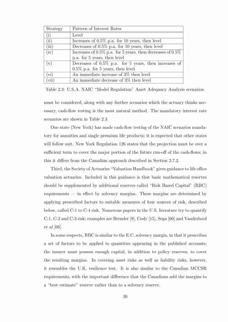
Strategy Pattern of Interest Rates
(i) Level(ii) Increases of 0.5% p.a. for 10 years, then level(iii) Decreases of 0.5% p.a. for 10 years, then level(iv) Increases of 0.5% p.a. for 5 years, then decreases of 0.5%
p.a. for 5 years, then level(v) Decreases of 0.5% p.a. for 5 years, then increases of
0.5% p.a. for 5 years, then level(vi) An immediate increase of 3% then level(vii) An immediate decrease of 3% then level
Table 2.3: U.S.A. NAIC “Model Regulation” Asset Adequacy Analysis scenarios.
must be considered, along with any further scenarios which the actuary thinks nec-
essary, cash-flow testing is the most natural method. The mandatory interest rate
scenarios are shown in Table 2.3.
One state (New York) has made cash-flow testing of the NAIC scenarios manda-
tory for annuities and single premium life products; it is expected that other states
will follow suit. New York Regulation 126 states that the projection must be over a
sufficient term to cover the major portion of the future run-off of the cash-flows; in
this it differs from the Canadian approach described in Section 2.7.2.
Third, the Society of Actuaries “Valuation Handbook” gives guidance to life office
valuation actuaries. Included in this guidance is that basic mathematical reserves
should be supplemented by additional reserves called “Risk Based Capital” (RBC)
requirements — in effect by solvency margins. These margins are determined by
applying prescribed factors to suitable measures of four sources of risk, described
below, called C-1 to C-4 risk. Numerous papers in the U.S. literature try to quantify
C-1, C-2 and C-3 risk; examples are Brender [9], Cody [15], Sega [60] and Vanderhoof
et al [66].
In some respects, RBC is similar to the E.C. solvency margin, in that it prescribes
a set of factors to be applied to quantities appearing in the published accounts;
the insurer must possess enough capital, in addition to policy reserves, to cover
the resulting margins. In covering asset risks as well as liability risks, however,
it resembles the U.K. resilience test. It is also similar to the Canadian MCCSR
requirements, with the important difference that the Canadians add the margins to
a “best estimate” reserve rather than to a solvency reserve.
36

Asset class Factor
U.S. Government issue bonds 0.0%Bonds rated AAA – A 0.3%Bonds rated BBB 1.0%Bonds rated BB 4.0%Bonds rated B 9.0%Bonds rated C 20.0%Bonds in default 30.0%
Residential mortgages in good standing 0.5%Residential mortgages 90 days overdue 1.0%Commercial mortgages in good standing 3.0%Commercial mortgages 90 days overdue 6.0%Mortgages in foreclosure 20.0%
Unaffiliated common stock 30.0%Unaffiliated preferred stock bond factor + 2.0%Real estate (investment) 10.0%Real estate (foreclosed) 15.0%Cash 0.3%
Table 2.4: U.S.A. NAIC Risk Based Capital factors for C-1 risk.
In 1992, the NAIC adopted RBC for life assurers’ financial reporting. The factors
given below are those of the NAIC.
C-1 (Asset) Risk. C-1 risk is the risk of loss on the life assurer’s assets. The
importance of fixed-interest and mortgage-type assets is reflected in the level
of detail at which the factors vary. For completeness, the factors are shown in
Table 2.4.
C-1 factors are applied to the book values of the relevant assets, except in
some of the riskiest categories such as bonds in default, for which the market
value is used.
The RBC margins for bonds are adjusted to allow for the concentration of the
funds in each class, and the margins for mortgages are adjusted to allow for
the assurer’s default and foreclosure experience relative to an industry average.
The total C-1 margin is the sum of margins for each asset category, further
adjusted for concentration in such a way that the margins for the ten largest
asset classes are effectively doubled.
The C-1 risk factors were derived from studies of the distributions of default
37

Sums at risk Factor
First $500,000,000 at risk 0.150%Next $4,500,000,000 at risk 0.100%Next $20,000,000,000 at risk 0.075%Sums at risk over $25,000,000,000 0.060%
Table 2.5: U.S.A. NAIC Risk Based Capital factors for C-2 risk.
Type of portfolio Factor
Low risk portfolio 0.5%Medium risk portfolio 1.0%High risk portfolio 2.0%
Table 2.6: Examples of U.S.A. NAIC Risk Based Capital factors for C-3 risk.
losses among the different asset types. For example, the bond factors are
intended to cover 92% of the expected losses in each category and 96% of the
expected losses for the whole bond portfolio, while the 30% factor for common
stock is supposed to cover the largest loss likely over a 2-year period with 95%
probability.
C-2 (Insurance) Risk. C-2 risk is the risk from excess claims. For individual life
assurance the factors in Table 2.5 are applied to the sums at risk.
Clearly these factors are similar in intention to the “sum at risk” component
of the E.C. solvency margin. Although the RBC factors are generally lower
than the E.C. margin, the E.C. formula for the total margin is simpler and
might be regarded as implicitly covering other risks for which RBC accounts
explicitly.
The aim of the C-2 factors is to meet excess claims over a 5-year to 10-year
period with 95% probability.
C-3 (Interest Rate) Risk. In U.K. terms C-3 risk is the mismatching risk. The
factors depend on the surrender rights and guarantees granted to the poli-
cyholder — a matter of importance in the U.S.A. — and on the degree of
cash-flow matching of the assets and liabilities. Table 2.6 shows some exam-
ples of the factors to be applied to the policy reserves.
A “low risk” portfolio, for example, is one in which the policyholders have
38

no surrender guarantees and the difference between the volatility of the assets
and liabilities is less than 0.125. Unless the insurer certifies that its asset and
liability cash-flows are well matched, the factors are increased by 50%.
C-4 (Business) Risk. C-4 risk is a “catch-all” category covering everything from
bad management to bad luck. The same factors are applied to all companies;
there is no attempt to pick out particular companies at greater risk than others.
The factors are 2% of life and annuity premium income and 0.5% of accident
and health premium income.
The total margin allows for correlations between C-1 and C-2 risk as follows:
Total margin =((C-1 + C-2)2 + C-32
) 12 + C-4
The office may employ statutory capital and surplus, an asset valuation reserve,
voluntary investment reserves and 50% of policyholders’ dividend (bonus) liabilities
(called Total Adjusted Capital) to meet the RBC margin. The ratio of the Total
adjusted Capital to the RBC margin must be at least 200%. (The factors given
above are 50% of their original (1992) values; the change was made on cosmetic
grounds, so that the published ratios should not attract adverse attention.) Below
200%, the company must file a recovery plan. Below 150%, the Insurance Commis-
sioners office will inspect the company. Below 100%, the company may be put into
“rehabilitation”. Below 70%, and the company must be put into rehabilitation. In
addition, if this ratio is between 200% and 250%, but on the basis of trend could
fall below 190% during the year, the company must file a recovery plan.
Several factors indicate that the RBC approach is more suited to U.S. than to
European conditions.
1. The basic reserving standard in the U.S.A. tends to be weaker than in E.C.
territories, and the RBC requirements allow for this. The JAWP quoted an
estimate by a U.S. actuary that the basic reserves might give 85% confidence
of meeting liabilities, while the reserves plus RBC might increase this to 95%.
Under current legislation most European insurers would have to set up stronger
reserves before the addition of solvency margins.
39

2. Insurance business in the U.S.A. is more homogeneous than insurance business
in the U.K., let alone the entire E.C.; therefore a prescriptive regime might
have a better chance of success in the U.S.A..
3. The detailed nature of the RBC analysis means that RBC is very office-specific.
That is, different offices might face quite different RBC requirements. (The
U.K. regulations have a similar effect in practice.)
4. The RBC factors based on the assets would penalise offices with adequate free
assets, especially if these were invested in equities. Some method of appor-
tioning assets to lines of business (as in the U.K. valuation regulations), and
of excluding free assets, would be required.
5. U.K. life assurers face different risks from U.S. life assurers, particularly with-
profit offices with substantial equity investments. These offices are subject to
a “negative risk” to the extent that they can vary future bonus; it is not clear
how this should be incorporated into a system of RBC. Three possible risk
factors are (i) the equity content of the relevant assets, (ii) the maturity of the
portfolio, and (iii) the extent of the terminal bonus cushion.
RBC is more prescriptive and (ostensibly) more sophisticated than E.C. solvency
regulation. The RBC factors were determined after detailed studies of the historic
variability of the various risks, but the underlying basis of RBC is still a traditional
valuation reserve. Indeed, it is acknowledged that RBC covers catastrophic risks
— the relatively short-term risks of uncovering the policy reserves — rather than
superceding the underlying valuation model. But broadly, it combines the aims of
the U.K. resilience test and the E.C. solvency margin.
2.7.2 Canada
New Canadian regulations in 1978 replaced mandatory valuation assumptions with
“appropriate” assumptions, to be decided by the Valuation Actuary. It became ap-
parent that actuaries were using a wide range of “appropriate” assumptions, and
there was concern that competitive pressure was eroding solvency standards. For
40

these and other reasons, the Department of Insurance Canada commissioned a re-
port from Dr. A. Brender on the establishment of a set of solvency margins (called
“Minimum Continuing Capital and Surplus Requirement” (MCCSR)). The result-
ing recommendations encompassed a system of factors similar to (but predating)
the RBC factors described in Section 2.7.1. An extended set of factors was subse-
quently adopted by the Canadian Life and Health Insurance Association (CLHIA)
as a measure of solvency which could be used to apportion the costs of a policyhold-
ers’ guarantee fund. Factors based on this extended set were then adopted by the
regulators. The MCCSR is thus a static test, with statutory force.
A separate reason for change was the adoption of GAAP reporting in Canada.
This led to the introduction of the “policy premium reserve” method of calculating
the basic policy reserves, broadly a gross premium method on a “best estimate”
basis, and likely to be inadequate by itself for solvency purposes. The Canadian
Institute of Actuaries (CIA) set up a Committee on Solvency Standards for Finan-
cial Institutions to consider what additional standards might be made necessary by
this move. It quickly concluded that no formula would do, and recommended that
Dynamic Solvency Testing (DST) — cash-flow scenario projections — should be
adopted as a standard by the CIA.
The standard as it has developed has several interesting features.
1. A number of mandatory scenarios, encompassing mortality, lapse, expense and
interest rate risk, are prescribed, but the actuary must use such additional sce-
narios as are required. The basic idea is not to subject the financial institution
to a rigid test but to explore its sensitivities.
2. Projections including 5 years’ future new business are required.
3. The measure of “adequacy” in each future year is ability to meet the projected
MCCSR. Instead of requiring cash-flow projections of run-offs (like New York
Regulation 126), the basis of DST is a traditional solvency valuation (plus
MCCSR margins). It might be described as a hybrid between the traditional
valuation and true cash-flow testing.
The CIA hopes to develop DST to make it independent of arithmetic formulae.
41

2.7.3 The Australian valuation proposals
A useful summary of the Australian proposals is included in Scott et al [59]. Broadly
it consists of four layers: (i) a Best Estimate Liability (BEL), (ii) Planned Margins
for Profit (PMP), (iii), a Solvency Reserve (SR), and (iv) a Capital Adequacy Re-
serve (CAR). The first two will also form the basis of profit reporting and taxation.
The main features are described below.
Best Estimate Liability. The BEL is a discounted cash-flow reserve on a best
estimate basis, in the sense that best estimates of future expenses, mortality
and lapses must be used. The rate of discount is also described as “best esti-
mate”, but with upper limits on the assumed yields on equities; for example,
for Australian equities the limit is the yield on 10-year bonds plus 5%. The
BEL must reserve for supportable bonuses, including terminal bonuses, which
are defined as bonuses resulting in nil profit under the BEL calculation basis.
Planned Margins for Profit. Profit is deemed to be earned when a risk is under-
written or a service provided, and the PMP are deemed to emerge when the
corresponding profit is earned. All expected future profits must be included in
the PMP. In this way the capitalisation of future profits at inception or on a
change of basis — often held against gross premium valuations — is avoided.
Solvency Reserve. The solvency reserve requires several contingencies to be con-
sidered. In particular, a set of factors are laid down, which must be applied to
the BEL best estimate assumptions and the BEL recalculated, allowing for any
discretions which the office may possess in (for example) varying charges; and
a resilience reserve must be held. The parameters of the resilience test include
a rise of 1.25% in gross equity yields and a change of ±1.5% in gross fixed-
interest yields. In addition, reserves must be held in respect of inadmissible
assets. The SR will be published.
Capital Adequacy Reserve. The CAR resembles the solvency margin but it is to
be calculated not on a “minimum” but on an “appropriate” basis — which is
partly at the actuary’s discretion. For example, the parameters of the resilience
42

test include a rise of 2.5% in gross dividend yields and a change of ±2.5% in
gross fixed-interest yields. The CAR will not be published, but will be disclosed
to the supervisor in confidence.
Failure to meet the CAR requirement would result in closer scrutiny by the
supervisor, while failure to cover the SR would result in intervention.
In part these proposals are driven, as in Canada, by the desire to define reserves
which can be used for accounting purposes, and then to base solvency reporting on
the same reserves by means of additional margins. In the U.K., the Joint Actuarial
Working Party favoured a similar approach, so we must turn again to the question
of how effective is the combination of traditional valuation reserve plus prescribed
margins
43

Chapter 3
Stochastic studies of life assurance
solvency
3.1 Introduction
The traditional valuation model, as a determinant of solvency, has been subjected
to scrutiny in recent years as stochastic models have been more widely explored.
Stochastic models of mortality and morbidity have been developed by statis-
ticians and actuaries and used to investigate the effect on cash-flows and profits
of random variation in the demographic experience. On the whole, though, such
randomness makes little impact provided the number of lives assured is reasonably
large (see Frees [25]).
Stochastic models have also been developed for asset yields and prices. This is
different in kind from modelling mortality stochastically, since the investment risks
in respect of different contracts are not independent, and might be more significant
for life assurance savings business. The “Principle of Insurance” does not apply to
the assets.
Since it was introduced to the profession in the U.K. by the Maturity Guarantees
Working Party [6], stochastic modelling has met a mixed response. It suggests
answers to important questions which are otherwise intractable, but the variability
of modelled quantities can be alarmingly large. The results depend, of course, upon
the model’s assumptions, and some would say that the assumptions underlying the
44

models of the assets most often used today are not sound enough to give credence to
a cash-flow model which uses them. One might therefore suspend judgement until
more convincing asset models are developed.
If, however, volatility is anything like that suggested by simple stochastic models,
we stand to learn a good deal from such research. It might be difficult to establish
results in absolute terms — for example it might be unwise to take as accurate an
estimated ruin probability — but there are other, more reasonable approaches.
1. The magnitude of the fluctuations in key life office statistics is of interest in its
own right. If it should be broadly similar when different models of the assets
are used, then this would be a major qualitative result. It might be argued
that instability rather than stability is the chief feature of modern life office
finance, so actuaries should be looking out for tools with which to measure
instability.
2. Comparative studies can be carried out, in which the effects of different actions
are compared using the same model of the assets and (if simulation is used)
the same set of investment scenarios. Relative results might be more credible
than absolute results.
In this thesis we work along the lines of the second of these approaches.
In this section we review previous work on life office solvency based upon versions
of the Wilkie model or its predecessor, and consider some questions suggested by
this work. Of particular interest is the development of strategies to model asset
allocation and bonus distribution. The papers considered are:
1. The Maturity Guarantees Working Party (1980).
2. The Faculty of Actuaries Solvency Working Party (1986).
3. The Faculty of Actuaries Bonus & Valuation Research Group (1989).
4. M. D. Ross (1991).
5. M. D. Ross & M. R. McWhirter (1991).
45
6. The Finnish Life Assurance Solvency Working Party (1992).
The papers listed above have used progressively more sophisticated — and pos-
sibly more realistic — strategies. It would be interesting to know if strategies which
proved to be effective in controlling, for example, the solvency of an office might
also appear to be realistic to a practitioner, or whether on the contrary, “realistic”
strategies were ineffective.
Other papers which have explored stochastic modelling but which are not directly
relevant are Purchase et al [54] and Hardy [29].
3.2 The Wilkie asset model
Since all but one of the papers described here use the Wilkie asset model or a variant
of it, we will describe it briefly first. A full description is given in Wilkie [68].
The model consists of four discrete (annual) time series generated by four se-
quences of independent unit normal random variables QZ(t), Y Z(t), DZ(t) and
CZ(t). These provide annual values of the Retail Prices Index (“RPI”), an in-
dex of gross equity dividends, the current running gross dividend yield, and the
gross yield on Consols, as follows:
1. Q(t) — Retail Prices Index
log
(Q(t)
Q(t− 1)
)= 0.05 + 0.6
{log
(Q(t− 1)
Q(t− 2)
)− 0.05
}+ 0.05QZ(t)
2. D(t) — An index of gross equity dividends
log(D(t)/D(t−1)) = 0.8DM(t)+0.2 log
(Q(t)
Q(t− 1)
)−0.0525Y Z(t−1)+0.1DZ(t)
where
DM(t) = 0.2 log
(Q(t)
Q(t− 1)
)+ 0.8DM(t− 1)
3. Y (t) — Gross dividend yield
log(Y (t)) = 1.35 log
(Q(t)
Q(t− 1)
)+ Y N(t)
where
Y N(t) = log 0.04 + 0.6{Y N(t− 1)− log0.04}+ 0.175Y Z(t)
46
4. C(t) — Gross yield on Consols (irredeemable fixed-interest securities)
C(t) = CM(t) + CN(t)
where
CM(t) = 0.05 log
(Q(t)
Q(t− 1)
)+ 0.95CM(t− 1)
and
log(CN(t)) = log 0.035 + 0.91 log
(CN(t− 1)
0.035
)+ 0.165CZ(t)
and with the constraint that C(t) can never be less than 0.05%.
The parameters given above are those of the “Reduced Standard Model”.
3.3 The Maturity Guarantees Working Party
The Maturity Guarantees Working Party (“MGWP”) of the Faculty of Actuaries
and Institute of Actuaries was set up to study the reserving requirements of equity-
backed unit-linked business with minimum maturity or surrender guarantees. Con-
cern had arisen following the insolvency of several small life assurers in the wake of
the stock market crash of 1974.
The MGWP’s report [6] put forward a method of reserving rather than a sug-
gested level of reserves, and in a break with the past the method used stochastic
simulation. For this purpose a model of equity prices and dividends was devel-
oped by Wilkie [6, Appendix D] — this model was later developed into the more
comprehensive model described in Section 3.2 above and in Wilkie [68].
The MGWP modelled a portfolio of regular premium business of terms from 10
years to 30 years. Premiums were invested in units whose prices were modelled by
the sample paths of the share price model with dividends reinvested. The maturity
value under each policy was guaranteed to be not less than the total premiums
paid. The outcomes of each simulation were the undiscounted and discounted totals
of the payments necessary to meet the guarantees — these represented the reserves
which would be needed under that scenario. In the basic projections, no further new
business was written.
47

The results based upon 5,000 simulations were that the distribution of maturity
guarantee reserves was very long-tailed. Only 1,539 cases required a non-zero re-
serve, and in 1,333 of these cases the discounted reserve was under 1% of the total
guaranteed amounts. However, the discounted reserve needed to ensure “solvency”
with 99.9% certainty was 16% of the total guaranteed amounts, and a discounted
reserve of 4% of the total guaranteed amounts was insufficient in about 98% of the
simulations. These results were enough to cause life offices to stop transacting unit-
linked business with maturity guarantees, at least until derivative securities became
more widely available.
In addition, the MGWP tested the sensitivity of the results to changes in the the
asset model and in the mix of business in the portfolio [6, Appendix E]. Two such
results are summarised here, since they are to some extent also typical of projections
of with-profit business.
1. If a single generation of contracts was considered (i.e. maturing in a single
year) then the number of simulations in which guarantee payments were made,
and the reserves required to meet any level of ruin probability, declined sharply
as the policy term increased. Some examples are shown in Table 3.7.
2. Most of the guarantee claims with the standard portfolio occurred in the first
few years of the projection, largely because of the much greater tendency of
short-term policies to give rise to such claims.
The importance of the MGWP’s report lies in its premise that solvency reserves
in respect of asset risks should be established by stochastic methods, and in the
example it gave of a practical method of estimating reserves, including steps towards
the introduction of a suitable asset model. It was perhaps fortunate that the problem
which presented itself did not require the consideration of investment and bonus
strategies.
3.4 The Faculty Solvency Working Party
The Faculty of Actuaries Solvency Working Party (“FASWP”) in 1986 carried out
stochastic projections of non-profit and with-profit business using the Wilkie asset
48

Policy term 5 Yrs. 10 Yrs. 15 Yrs. 20 Yrs. 25 Yrs. 30 Yrs.
No. of simulations(of5,000) with guaran-tee payments
1,127 567 297 147 54 25
Undiscountedreserve, 0.5% ruinprob.
45% 42% 42% 34% 29% 13%
Undiscountedreserve, 5% ruinprob.
32% 26% 20% 8% 0% 0%
Discounted reserve,0.5% ruin prob.
37% 28% 23% 16% 11% 4%
Discounted reserve,5% ruin prob.
26% 18% 11% 4% 0% 0%
Table 3.7: Maturity Guarantees Working Party — Number of simulations withguarantee claims at terms 5–30 years, and solvency reserves as % of total guaranteedamounts
model [37], [68]. Some of the features of their investigations were as follows:
1. Each set of projections followed a single tranche of 20-year endowment policies
from inception to maturity in 1,000 scenarios.
2. The underlying assets were assumed to be invested either
• 100% in equities, or
• 100% in gilts, or
• 50% in each of equities and gilts (by market value).
In those projections in which non-profit business was invested 100% in gilts
the liabilities were immunized if possible, using irredeemables or dated gilts.
3. Two bonus strategies were used for the with-profit endowments.
• The first strategy was based upon a passive net premium “valuation for
surplus”. Surplus was calculated by accumulating the premiums less
claims at the earned rate of return, ignoring capital appreciation or de-
preciation, and comparing this with a 3% net premium reserve. If the
49

surplus was positive, it was used to provide one year’s bonus; if negative,
no bonus was declared.
This method led to moderate bonus rates, initially with very low standard
deviations, which steadily increased during the 20 years of the projection.
Only in the last years of the projections and only with 100% equity in-
vestment did the standard deviation of the bonus rate exceed half the
mean bonus rate.
• The second strategy used a more realistic active bonus reserve approach.
Assets were valued on a notional basis, gilts by applying a 5-year average
of the net gilt yield to the future gilt income, and equities by applying
a 5-year average of the dividend yields to the current level of dividend
income. The interest rate used to value the liabilities was based either
on the 5-year average of the net gilt yield, or on the 5-year average of
the net dividend yield plus the difference between the 5-year averages of
the gross and net gilt yields (the latter adjustment being to allow for the
experienced growth rate in equities). A bonus rate was declared which
would, if maintained until the business had run off, just exhaust the assets
valued as above. (The FASWP did not state whether this strategy was
modified in case the market value of the assets exceeded their notional
value, particularly in the last few years of the projection.)
The mean bonus rates given 100% gilt investment were very similar to
those emerging under the passive strategy, but with a more stable stan-
dard deviation. The mean bonus rates which emerged given either 50%
or 100% equity investment were much larger than those emerging under
the passive strategy, and had much larger standard deviations.
Note that the active bonus strategy was regarded by the FASWP as being
more realistic than the passive bonus strategy.
4. The FASWP calculated a “solvency reserve” in each year of each simulation,
equal to the assets which would have to be held at the end of that year to meet
the future liabilities as if the outcome were known in advance. The solvency
50

reserve was compared with the market value of the assets, with the statutory
minimum valuation reserve and with a gross premium valuation reserve. The
FASWP did not display ruin probabilities explicitly, but it was possible, from
those cases in which the solvency reserve exceeded the market value of the
assets, to deduce roughly where the dangers of insolvency lay. At the 5%
level, only the with-profit business, invested 100% in gilts and using the active
bonus strategy, came close to being solvent. If the with-profit business was
invested either 50% or 100% in equities, and if the active bonus strategy was
used, the mean margin required over the market value of the assets was positive
in every year of the projection. That is, the mean position in every year under
the 1,000 simulations was one of actual insolvency. The FASWP commented
that
“The reason for these disquieting results lies not so much in the
bonus distribution policy actually followed, but more particularly in
the assumption that the policy will be rigidly adhered to regardless
of future conditions.”
In other words, the bonus strategies were dynamic but not dynamic enough.
5. Other factors which ought to be taken into consideration are:
• The projections did not allow for any additional estate which the office
might possess. “Additional estate” is here taken to mean any excess
of assets over policyholders’ total asset shares; some authors call it the
“orphan surplus”.
• There was no allowance for continuing new business. Such an approach
was dictated by the aim of studying solvency assuming, as usual, an office
closed to new business, but it might be expected that new business, and
new business expansion, would have had a significant effect.
• The investment strategy was entirely passive, except that non-profit busi-
ness might be immunized. Otherwise, there was no attempt to relate the
investment strategy to the nature or term of the guarantees.
51

• There was no terminal bonus strategy, except that the active bonus strat-
egy might be described as aiming for a target terminal bonus of nil.
• The FASWP did not comment upon the individual sample paths of any
of the projections
3.5 The Faculty Bonus and Valuation Research
Group
The Faculty of Actuaries Bonus and Valuation Research Group (“FABVRG”) in
1989 [22] modelled 20-year with-profit endowment business under conditions of de-
clining investment returns, and inter alia studied the stochastic effects of the Wilkie
investment model. The stochastic parts of their work fell into three parts.
The first two parts concerned the distribution of maturity values or bonus rates
in the financial conditions generated by the Wilkie model, ignoring valuation con-
siderations, and are not directly relevant here. One point of interest was the inves-
tigation of “declining Equity Backing Ratio (EBR)” investment strategies, in which
the assets underlying a contract are switched progressively from equities to gilts as
maturity approaches.
In the part concerned with solvency, the FABVRG first carried out deterministic
projections where investment conditions were represented by the Wilkie model with
the stochastic fluctuations removed. These showed the effect of assuming that the
mean values of the stochastic asset model (approximately) held in future. They
went on to restore the stochastic components of the Wilkie model and examined (in
10 simulations) how large the fluctuations in several key statistics, including some
measures of solvency, might be. New business was allowed for, growing at 2.5% over
the rate of inflation each year. The office was assumed to have an additional estate
at outset of 30% of the asset shares.
Only one investment strategy was used, namely investing the fund 70% in equities
and 30% in gilts every year.
A fixed bonus strategy (a single tier bonus declining from 5% to 3.5% over the
first 5 years of the projection) and two dynamic bonus strategies were considered.
52

Valuation of FASWP FABVRG
gilt income 5-year average gilt yield Fixed 7.5%dividend income 5-year average dividend
yieldFixed 7.5% with 4%dividend increases
liabilities backed bygilts
5-year average gilt yield Fixed 7.5%
liabilities backed byequities
5-year average dividendyield + difference be-tween 5-year averagegross and net gilt yields
Fixed 7.5%
Table 3.8: Comparison of valuation assumptions used by the Solvency WorkingParty and the Bonus & Valuation Research Group of the Faculty of Actuaries
1. First, the liabilities were valued at a fixed interest rate of 7.5% net, on a gross
premium basis allowing for inflation of future expenses at 5%. Then the future
net income on the assets was also valued at 7.5% net. Equity dividends were
assumed to increase at 4% per annum (a rate broadly consistent with the trend
in the Wilkie asset model). The resulting surplus was used to declare a rate
of bonus which could be maintained until all the in-force business had run off.
Table 3.8 compares this method with the active bonus strategy used by the
FASWP.
So although the FABVRG adopted a dynamic bonus strategy, it was based
upon fixed yields for valuing both assets and liabilities, taking no account
of current conditions, in contrast to the FASWP method. The strategy was
dynamic, but less so than the method which the FASWP had described as too
rigid.
2. Two patterns of bonus were considered. Either (i) a single tier bonus was
declared, or (ii) a two-tier bonus under which the rate of bonus on sums assured
was fixed at 2%, and the rate of bonus on bonus was allowed to fluctuate. The
latter showed much higher fluctuations in the bonus rates which emerged; it
suffered from the first tier of 2% being fixed, as there were instances of the
second tier falling to nil, while none of the single tier bonuses fell to nil.
Key statistics were graphed, although with 10 simulations this served only to
give an impression of the fluctuations around the deterministic trend lines. The
53

quantities graphed were:
1. The ratio of assets to asset shares (A/AS ratio). This measured the rate at
which the office added to or drew upon its free assets. Broadly speaking, low
rates of expansion caused it to increase, and high rates of expansion caused it
it decline towards a value of 1.0. Several projections showed it falling below
1.0.
2. The ratio of assets to the statutory minimum liabilities (A/L ratio). This
represented the statutory solvency position of the office. The fluctuations in
this ratio were very large. To some extent this may have been because of the
uncontrolled strategies which were being pursued, but it is partly due to the
differing volatilities of the assets at market value and the liabilities on a net
premium basis. Note that no resilience reserve was included in the liabilities.
3. The emerging terminal bonus rates. These showed very large fluctuations. The
deterministic trend of terminal bonuses was towards a rate of about 10% to
20% of the guaranteed liabilities, but even at very long durations the emerging
rates varied between 0% and about 150% of the guaranteed liabilities. What
was also interesting was the magnitude of the fluctuations over quite short
periods within a single simulation, in the absence of any attempt to smooth
maturity values.
Similar graphs showed the effect on 10 simulations of a burst of rapid growth of
new business; the main effect was to reduce the A/AS ratio to 1.0 very quickly, and
to make it almost impossible for the office to maintain its additional estate.
Points to consider when evaluating the methods used by the FABVRG are:
1. Investment strategies were fixed.
2. The dynamic bonus strategies were only partly dynamic in the sense that the
algorithm was not a function of either historic or current conditions.
3. The dynamic bonus strategies were based on reversionary bonus only, and did
not attempt to control terminal bonuses in any way. In effect, the terminal
bonus target was nil as in the dynamic strategy used by the FASWP.
54

4. The office modelled was open to new business and had an additional estate.
This was therefore a model of commercial adequacy rather than solvency, and
the FABVRG introduced the A/AS and A/L ratios as appropriate indicators
of the office’s position.
5. Solvency was represented by the A/L ratio, and there was no attempt to relate
this to solvency on a run-off basis, as had been done by the FASWP.
6. The office was assumed to pay out the full asset share where this exceeded
the guaranteed benefits at maturity; there was no attempt to smooth terminal
bonuses or to reserve for the cost of meeting the guaranteed benefits when the
asset share was insufficient.
7. Only 10 simulations of the full office model were undertaken, and no statistical
analysis was carried out.
3.6 M. D. Ross
M. D. Ross in 1989 [57] described the difficulties of modelling management strategies,
in a paper dealing with his office’s approach to developing a “computerized actuary”
to “manage” a with-profit life office driven by a version of the Wilkie asset model.
In contrast to the simple portfolios of business considered by the FASWP and
the FABVRG, the model office included a “typical” mixture of annual and single
premium pensions policies. Future new business was allowed for, growing at 5%
per annum over the rate of inflation. Paid-up and surrendered contracts were also
allowed for. At the starting point (taken to be 1987) the office had an additional
estate of 25% of the asset shares, or 29% of the statutory minimum liabilities.
The most interesting developments were the bonus and asset allocation algo-
rithms.
1. The fundamental question of bonus policy was taken to be the relationship
between guaranteed benefits and terminal bonus. Reversionary bonus was set
by aiming for a global terminal bonus target of 40% of the projected guaranteed
liabilities. That is, reversionary bonus rates were declared so that the projected
55
payouts in respect of all the in-force business were about 71% guaranteed
benefits and 29% unguaranteed benefits in aggregate.
In order to project the benefits, the cash-flows arising in respect of (i) the assets
underlying the asset shares and (ii) the liabilities were valued consistently,
allowing for the then-current investment mix.
• The assets underlying each policy’s asset share were split into gilts and
equities by market value, in proportion to the office’s aggregate asset mix.
• Income arising from the gilt component of the asset share was valued
using the lower of (i) the long-term mean redemption yield from the
Wilkie investment model, and (ii) a 5-year average of the historic gilt
yields.
• Dividends on the equity component of the asset share were averaged over
the previous 5 years, allowing for indexing at the lower of (i) the mean
long-term rate of growth of dividends used in the Wilkie investment model
and (ii) a 5-year average of the historic rates of growth in dividends.
• The averaged dividends were then valued at the mean long-term dividend
yield used in the Wilkie model.
• Liability cashflows were valued using the lower of (i) the long-term yield
assumptions from the Wilkie investment model, weighted by the actual
asset mix on the valuation date and (ii) a 5-year average of the historic
investment return.
• A single tier compound bonus rate was declared so that the value of
the assets was 1.4 × the value of the liabilities, but with the overrid-
ing provision that if business with only 5 years to maturity supported a
lower reversionary bonus and no terminal bonus, then that lower rate of
reversionary bonus was declared.
Given premium rates for policies of different terms typical of those in U.K.
practice, this approach led to achieved terminal bonuses of more than 40% for
longer term policies, and of less than 40% for shorter term policies. This was
56
reflected in a greater tendency for the asset shares of short term policies to be
lower than their guaranteed benefits at maturity.
This bonus strategy added some sophistication to the method of the FABVRG.
It was no more dynamic in good times, because the rates of interest used to
value both assets and liabilities were then fixed at the long-term means from
the asset model — in principle no different from the FABVRG choosing a fixed
rate of 7.5%. However, in more depressed conditions the valuations were based
on 5-year averages of the historic yields, and this represented the influence of
current conditions on the judgement of the valuation actuary. The strategy
might be criticised for defaulting to the “correct” yields — the long-term mean
yields used in the asset model — therefore assuming that the actuary is using a
“correct” asset model. It would be preferable, if possible, to fit an appropriate
model to the yields experienced in each simulation.
2. Two investment strategies were used. The first was simply to invest 80% of
the fund (by market value) in equities at any given time, and the remaining
20% in gilts.
The second was a dynamic strategy based on the fact that the maximum valu-
ation interest rate permitted under the U.K. regulations can often be increased
by switching assets from equities to gilts (see Section 2.4). If the A/L ratio
(i.e. the ratio of assets to liabilities in respect of the whole office, where the
liabilities were calculated on the statutory minimum basis) fell below 1.25,
assets were progressively switched towards equities until, with the A/L ratio
at 1.05, the fund was invested entirely in gilts. (The limit of 1.05 allowed for
the fact that the E.C. solvency margins were not included in the minimum
liability.)
A similar investment strategy was used by the FABVRG in some later inves-
tigations which did not, however, employ a stochastic model (see Paul et al
[51]).
3. Some additional features of the model included the following:
• The premium rates were recalculated whenever the bonus earning power
57

of the current premiums (presumably on the basis described above) fell
below 1% per annum; then a premium calculated to support 1% per
annum was used instead. Single premium rates were recalculated each
year so that they supported the same bonuses as an annual premium
policy of the same term.
• Maturity values were based on only 98.5% of the asset shares, where these
exceeded the guaranteed liabilities. The remaining 1.5% represented the
charge for the guarantees.
• Executive Pension policies (about 45% of the portfolio) were made paid
up at a rate of about 4% per annum. Thus a significant proportion of
policies becoming claims might be paid-up.
• Executive Pension policies were surrendered at a rate of 2.5% per annum,
with surrender values based on 90% of the asset share, increasing to 98.5%
over the last third of their term. This suggests that there was a significant
contribution to the office from surrender profits; the effect of such profits
was not discussed.
100 simulations were carried out. Most of the results were in the form of graphs
over time of the 5%, 10%, 30%, 50%, 70%, 90% and 95% quantiles; in other words
whatever quantity was being observed, the 5th worst simulation at each time was
plotted, and the 10th worst, and so on. It is important to note that these did not
represent the paths followed by a single simulation; an office which spends most of
its time in the top decile may still visit the bottom decile occasionally.
The results for financial ratios and emerging bonus rates using the fixed invest-
ment strategy — 80% in equities — were not inconsistent with the graphs produced
by the FABVRG with their fixed strategy — 70% in equities — bearing in mind
that the FABVRG graphed 10 sample paths from 20-year ordinary endowments and
Ross graphed percentiles from a mix of pensions business. It is hard to make direct
comparisons
The comparison of the fixed and dynamic investment strategies was interesting.
The upper percentiles (representing the more favourable outcomes) were affected
very little; in these circumstances, the dynamic investment strategy would default
58

to 80% equity investment, the same as the fixed strategy. The lower percentiles
were generally lifted up to some degree. This was most striking in the case of the
A/L ratio, which was to be expected since the level of that ratio was the criterion
for changing the asset mix. Bonus rates appeared to be little changed , though the
frequency of a bonus rate of nil was actually increased under the dynamic investment
strategy.
The significant points brought out by this paper were:
1. This study was of an on-going office which continued to trade, like the model
of the FABVRG and unlike the model of the FASWP.
2. The investment strategy was based on the statutory minimum liabilities in-
cluding (roughly) the E.C. solvency margin but excluding the U.K. resilience
reserve. The need to satisfy the Regulations cannot be ignored so this was a
realistic choice.
3. The reversionary bonuses were driven by a global terminal bonus target, but
constrained by maturities in the near future. This was more realistic than
the FASWP in two respects: (i) the terminal bonus target was not zero, and
(ii) bonuses were based on a portfolio of in-force policies rather than a single
tranche of business. It also went some way to meeting a possible difficulty
with the FABVRG’s bonus algorithm, which was based on notional values of
the assets which might be less than the market values of the assets.
4. Asset and liability cash-flows were valued, where necessary, on a fixed basis,
but with a more realistic over-ride in adverse conditions. The fixed values used
in normal conditions were the long-term mean yields from the asset model; this
perhaps credits the actuary with too much knowledge.
5. Premium rates were dynamic, being altered if they lost too much bonus earning
power.
6. The asset shares were reduced by 1.5% at maturity by way of a charge —
apparently ad hoc — for the guarantees.
59

7. The model was considerably more complex than any of those used in the four
papers previously reviewed, not only in respect of its management algorithms
but also in respect of the business modelled. Comparison with other studies
is difficult.
8. The results were based on only 100 simulations.
3.7 M. D. Ross & M. R. McWhirter
In 1991, M. D. Ross and M. R. McWhirter investigated the impact of the restrictions
on equity yields in the U.K. statutory minimum valuation basis in a paper [58], which
was circulated privately. This paper used a model of a with-profits office which was,
in many respects, the most sophisticated yet described. First we will describe the
features of their model, and then we will summarise their results.
• The office wrote non-pensions with-profit endowment business of terms 5 years
to 30 years. The in-force in 1990 was built up using a comprehensive set of
assumptions. Rates of return were based on the Barclays de Zoete Wedd
indices; historic tax rates were used, and bonus rates and the growth of new
business were modelled in detail to represent a typical U.K. experience. The
office enjoyed a A/L ratio of 1.81 and a A/AS ratio of 1.20 in 1990, so was in
a position of some strength.
• By default, 80% of the fund by market value was invested in equities. For
purposes of comparison, a second strategy driven by statutory solvency was
used, in which assets were switched from equities to gilts progressively as the
ratio of assets to statutory liabilities fell from 1.30 to 1.08; the target A/L ratio
was considered to be a linear function r() of the proportion in equities such
that r(0.8) = 1.3 and r(1.08) = 0. The lower limit of 1.08 was used because
the E.C. solvency margins and the U.K. resilience reserves were ignored, and
because valuations were performed at the year-end before new business was
added on.
60

• The assets underlying policy asset shares were valued on a long-term basis
similar to that described above in Section 3.6. Also as in Section 3.6, the
yields used for discounting future cash-flows in calculating reverionary bonus
were based on the assumptions in the asset model, overridden during periods
of low returns.
• The two tiers of supercompound bonus were determined separately. The bonus
on sums assured was the bonus earning power of the new business, allowing for
a terminal bonus target of 30% over the new business as a whole. The bonus
on bonus was then the bonus earning power of the whole office, allowing for
the declared rate of bonus on sums assured and the 30% terminal bonus target.
There were two checks; the second calculation was repeated using only those
policies within 5 years of maturity and a zero terminal bonus target, and if the
resulting rate of bonus on bonus was lower it was declared instead; and if the
rate of bonus on bonus exceeded the rate of bonus on sums assured the bonus
was recalculated on an ordinary compound basis. Changes in reversionary
bonus from year to year were limited, the first tier to 0.3% and the second tier
to 0.5%, though the latter was sometimes adjusted in the light of the change
in the first tier. In some projections the terminal bonus target was changed
from 30% to 60%.
• Maturity payments were based on 98.5% of the smoothed asset shares (with
a minimum of the guarantees). The smoothing was carried out by revaluing
equity assets using a weighted 4-year arithmetic moving average dividend yield.
The values of gilts underlying the asset shares of maturing policies were not
smoothed.
• Gilts were all of term 15 years while the office remained open to new business,
reduced to 10 years and then 5 years after the office was closed. Therefore
the values of the gilts underlying maturing policies, being unsmoothed, might
increase the volatility of maturity payments.
• Premium rates and expenses were based on those used by Ljeskovac et al [39]
but in the case of premiums with the same override in conditions of low bonus
61

earning power described in Section 3.6.
• Lapse rates varied from 7.5% per annum at durations 1 – 5 years, to 1.5% per
annum at durations 21 years and over. Surrender values were 95% of the asset
share, increasing to 98.5% over the last third of their term, with minima of
70% and 75% of the premiums paid in years 1 and 2 respectively. Although
95% of the asset shares ought to contribute to ptofit, it is a higher proportion
than that apparently used in practice by many U.K. offices.
The authors modified the parameters of the Wilkie model, most significantly
to increase the force of inflation from 0.05 to 0.06 and to introduce real dividend
growth of 1.5%. The latter increased the expected returns on equities relative to
gilts, which some commentators have held to be too small under Wilkie’s original
parameterization.
The authors’ purpose was to show that the U.K. statutory valuation basis acts in
a manner detrimental to policyholders, by forcing life offices to switch from equities
to gilts at times when the offices might in fact be solvent in cash-flow terms. Their
approach was to carry out simulations under the original investment strategy (80%
in equities) and to record:
• the times at which statutory insolvency occurred (i.e. the A/L ratio fell below
1.08);
• the maturity values paid each year;
• the residual assets after the office had been closed and the business run off.
The simulations were re-run assuming that the office used the asset-switching
strategy dictated by statutory solvency, and the corresponding outcomes were recorded.
Only 50 simulations were carried out; 49 were stochastic and 1 was deterministic,
in which the variances in the Wilkie model were set to zero.
The main results of the stochastic runs were as follows:
1. Under the fixed investment strategy, 45 of the 49 simulations suffered statutory
insolvency during the first 40 years. About 10% of offices were insolvent at any
given time. However, only one simulation produced a deficit after 70 years.
62

2. Under the dynamic investment strategy the number of insolvencies fell to 11.
One simulation produced a deficit after 70 years, but not the same simulation
as before. The authors concluded:
“. . . this is a powerful argument for acceptance that the present val-
uation regulations are far too severe in terms of correctly identifying
situations in which an office might become “truly” insolvent.”
3. The “payout ratio” in each year in each simulation was calculated. This is the
ratio of the maturity values under the fixed and dynamic investment strategies
respectively; it is a measure of the extent to which the asset switching is bene-
ficial or detrimental to policyholders — at least in retrospect. The distribution
of the payout ratio was highly skewed towards values above 1.0. The median
payout ratio for all policy terms was above 1.0. For example, the mean of the
median payout ratios between 2011 and 2030 (20 and 40 years from outset)
was 1.017 at term 10 years, 1.15 at term 20 years, 1.26 at term 30 years and
1.322 at term 40 years. Note that this result might depend significantly upon
the assumption of real dividend growth. The authors concluded:
“In simple terms, the artificial restriction on equity yields not only
seriously damages the office’s health but policyholder’s expectations
and actual results as well.”
The payout ratio tended to revert to 1.0 after closure, because the equity
proportion tended to revert to 80% under the dynamic investment strategy,
indicating that the office had a considerable excess of assets when it closed.
4. The dynamic investment strategy increased the incidence of negative theoret-
ical terminal bonus rates — that is, calculated maturity values lower than
the guarantees. Thus the cash-flow solvency of individual tranches of policies
deteriorated, while the statutory solvency of the whole office over the 70 years
improved. The authors did not quantify the assets remaining after the run-off,
so it is not possible to say to what extent the office’s position was maintained
on a cash-flow basis.
63
5. Repeating the experiment with a terminal bonus target of 60% instead of 30%
cut the number of insolvencies to 14 under the fixed investment strategy and
1 under the dynamic investment strategy. The incidence of asset switching
under the latter was much decreased, and not surprisingly the payout ratios
were much closer to unity. However, the higher target resulted in very much
lower reversionary bonuses, including 7 simulations in which there was no
bonus on sums assured at all at least once in the first 40 years.
This approach applied the cash-flow solvency criterion of the FASWP to a more
sophisticated model, but for understandable reasons of space and computer time it
left many questions open.
1. The model office was extremely complex, being set up to reflect historical
conditions up to 1990. The effects of these conditions would have a major
bearing on the outcomes, at least during the first half of the projection. Of
the 45 insolvencies resulting from 80% fixed in equities and a 30% terminal
bonus target, 2 occurred in the first 5 years , 15 in the second 5 years, and
another 13 in the third 5 years. In no case did insolvency occur for the first
time after the office had been closed to new business. It is therefore difficult
to draw wider conclusions about the effectiveness of the statutory minimum
valuation basis.
2. The statutory minimum valuation was compared with cash-flow solvency by
allowing “insolvent” offices to continue in operation for 40 years, regardless
of whether statutory insolvency occurred sooner or later in the 40 years. Al-
though statutory insolvency appeared to be a poor test of the office’s ability
to meet its liabilities over this long time scale, it remains possible that that
an “insolvent” office would have had more difficulty in meeting its liabilities
had it been closed down at the time of insolvency. That is, after all, what a
traditional valuation attempts to determine. In this connection, the working-
through of the 1990 in-force might have led to different results upon earlier
closure. We will return to this point in Chapter 8.
3. The authors did not suggest a modfication of the statutory minimum valuation
64

basis, or an alternative to it, which would remedy the defects which they
described. However, the focus of their concern was clearly the restriction on
equity yields. They concluded:
“What remains fundamental, though, is that any valuation test
should not act to distort the asset mix of life offices and it is this
point that lies at the heart of this paper.”
3.8 The Finnish Solvency Working Group
In 1992 The Life Assurance Solvency Working Group (“LASWG”) in Finland re-
ported the results of an investigation to the Ministry of Social Affairs and Health
[55]. It had the task of
“. . . examining the need for the reform of the solvency regulations of
life assurance companies and on the basis of the examination draw up
proposals for change.”
The main features of the investigation were as follows:
1. The asset model was based on a first-order autoregressive model of the rate
of inflation but with parameters suited to Finnish conditions and a Gamma-
distributed noise term.
The asset categories modelled were (i) long-term loans and bonds (ii) short-
term loans and bonds (iii) common stock and (iv) property. Models for both
the income and price changes for these assets were based on the Wilkie model.
A new development was the simulation of a reference index representing the
growth of national product. If the index of share prices moved too far from the
reference index then the mean and standard deviation of the annual change in
the share price index were adjusted to bring it closer to the reference index.
Details were not reported in the English summary, but Pentikainen et al [52]
and Pukkila et al [53] are useful references.
65

The published simulations showed the effects of different initial distributions
of the assets in these categories. Subsequent asset allocations were governed
by an allocation rule which was not described in the English summary.
2. The bonus rule was based on the margin or level of surplus, i.e. the margin of
assets over mathematical reserves (elsewhere called the “additional estate”).
Four levels of surplus which acted as trigger points for the bonus rule, U0 ≤U1 ≤ U2 ≤ U3 were defined. The default for bonus rates was that they should
be equal to the rate of inflation, though not less than 0% and not more than
15%. (In Finland, the sum assured and the premium and the reserve — and
therefore also the loading for future expenses — are increased by the same
proportion. There is no terminal bonus.)
• U0 was the minimum margin (the estimation of which was one aim of
the investigation). If the actual margin U was below U0 no bonuses were
payable and it could be assumed that the supervisors were taking a close
interest.
• If the actual margin U was between U0 and U1 the rate of bonus was less
than the rate of inflation.
• If the actual margin U was between U1 and U2 the default bonus rule
applied.
• If the actual margin U was between U2 and U3 the rate of bonus was
greater than the rate of inflation.
• If the actual margin U was greater than U3 a bonus intended quickly to
return the margin to the U2 level was declared.
The application of the bonus rule therefore required (i) the definition and (ii)
the estimation of U0, the minimum margin.
Umin was defined to be that amount which, in addition to the policy reserves
and allowing for new business, would ensure that assets exceeded liabilities after 3
years with 97% probability. (This choice was influenced by the minimum margin
previously adopted for general insurance business, i.e. that assets should exceed
liabilities after 1 year with 99% probability.)
66

Umin was estimated as the solution of
(1 + α)Umin = 1.8(σ0(V + Umin)2 + (σ2)
2)0.5 − βV − Yr
where α represents the expected rate of return over 3 years on the assets held;
V is the mathematical reserve at outset; σ0(V + Umin) is the standard deviation of
the change in the office’s assets over 3 years; σ2 is the standard deviation of the
non-investment profits over 3 years; β is the expected rate of investment surplus
arising in respect of the mathematical reserves over 3 years, and Yr is the expected
non-investment profits arising over 3 years. The fractile value 1.8 was chosen after
carrying out simulations with models of different types of life office.
Note that in the estimation of Umin it was assumed that no future bonuses would
be paid — that is, in the 3-year simulations used to determine the fractile there were
no bonuses.
Umin was generally higher than the E.C. solvency margin if the asset mix tended
towards equities and real estate, and lower than the E.C. solvency margin if the
asset mix tended towards bonds and loans. Therefore, for the application of the
bonus rule described above (using the trigger points U0 ≤ U1 ≤ U2 ≤ U3) U0 was
taken to be the maximum of Umin and the E.C. solvency margin. The trigger points
U1, U2 and U3 were defined (following some experiments) as follows:
• U1 = U0 + D
• U2 = U0 + S + 2.7D
• U3 = U0 + S + 3.5D
where S is the shareholders’ equity and D is the estimated standard deviation
of the investment surplus arising over three years given a fixed asset mix. Note that
all 4 trigger points must be calculated as functions of current conditions each year.
Finally, the Group carried out simulations to test the effectiveness of the bonus
rule in conjunction with U0 defined as above. The main results were as follows:
1. The bonus rule was successful in steering surplus between the upper and lower
limits for different types of office (risk, savings and traditional business). In
none of the cases examined was there ever an insolvency.
67

2. In an office writing savings business, with mainly equity-type assets, surplus
tended to increase so that the upper trigger points were predominant in forcing
the distribution of surplus. However, in an office writing savings business, with
mainly fixed-interest type assets, surplus tended to stay close to the lower limit
U0 and there were many years without bonuses. In both cases the office was
assumed to expand fairly rapidly.
3. In a traditional office, invested mainly in equity-type assets, not expanding
rapidly, but with moderately high inflation (mean 8% per annum) the surpluses
were fairly evenly spread between the lower and upper trigger points U0 and
U3, but tended to change rapidly. The bonus rule was nevertheless successful
in ensuring solvency.
4. In a traditional office, invested mainly in equity-type assets, not expanding
rapidly, but with low inflation (mean 4% per annum) and a correspondingly
lower mean rate of return, the surplus tended to rise to the upper limit U3.
The main interest in this work is the definition of a solvency margin and a
bonus rule which ensure solvency in a variety of circumstances without making use
of terminal bonus. However, “solvency” was still defined in terms of a traditional
valuation reserve. Further, the report did not compare payouts with asset shares
so it was not possible to tell whether or not the success of the system depended
on retention of surpluses which would be regarded as distributable under the U.K.
system of asset shares and terminal bonuses.
3.9 Conclusions
The papers reviewed above introduce a number of ideas.
1. Problems of insurance solvency related to asset risk may be modelled empiri-
cally, given a stochastic model of the assets (MGWP, FASWP).
2. In some cases, managers have considerable discretion over decision making. Ig-
noring that discretion in the modelling raises doubts about the results (FASWP).
68

3. Investment strategies have to be suited to the assets available locally, but
might be driven by considerations of portfolio selection (LASWG) or solvency
(Ross).
4. Bonus rules have to be suited to local practice, but might be driven by retro-
spective surplus (FASWP) or prospective solvency (FASWP, Ross, LASWG).
5. Explicit cash-flow projections of closed offices provide a standard to which
other methods of assessing solvency can be compared, either in whole or in
part (Ross, Ross & McWhirter).
6. The models considered include single generations of business (MGWP, FASWP),
run-offs of a closed office with a realistic mix of business (MGWP, Ross) and
projections allowing for future new business (MGWP, Ross & McWhirter,
LASWG).
The results of each investigation differed, being specific to (i) the details of the
offices being modelled, and (ii) the asset models used. This points to a possibility
which could be of great significance: that it might be difficult to prescribe detailed
and uniform rules for solvency assessment rather than general methods. In the U.K.,
this means abandoning the ideal of openness to external checks (through the data
in Schedule 5 of the D.T.I. Returns), but that ideal is in practice being abandoned
anyway. In other territories, it might mean less prescriptive approaches to solvency
reporting, and more responsibility for individual actuaries.
The details of each model include the asset allocation and bonus rules, being
themselves models of the actions of future managers. Given the discretions described
in Chapters 1 and 2, it is hard to see how uniform rules will lead to a proper
supervision of PRE, as opposed to strict solvency.
This thesis will look at some aspects of managers’ discretions, mainly over asset
allocation (Chapter 5) and benefit smoothing (Chapter 6). Then in Chapters 7 and
8 we will look at the effectiveness (or otherwise) of prescriptive solvency valuations
in the case a particular model office. We will illustrate that in modern circumstances
the imposition of uniform standards based on the traditional model might not be
an effective or a consistent measure of solvency.
69

Chapter 4
A simple model office
4.1 Introduction
This chapter describes a very simple model office which will be used later to study
different asset allocation rules, bonus rules and traditional valuation tests. The main
simplification is to restrict the model to 10-year with-profit endowment contracts,
for two reasons:
1. Simulation is computationally intensive, and shorter terms help to save com-
puter time.
2. As a rule, short-term business is more sensitive to asset volatility than long
term business — at least, given pricing assumptions typical of those in use in
the U.K. — and therefore shows more clearly the impact of a stochastic asset
model and the effects of asset allocation and bonus rules.
To introduce the model, we will illustrate the sample paths of simulations of
various outputs, including measures of solvency, and we will investigate in more
detail the circumstances which cause statutory insolvency in the model.
The model of this chapter will be called the “baseline” office in subsequent chap-
ters. Some of the assumptions described below, and projections based upon them,
have appeared in [43]. Here they are taken as starting points for the study of alter-
natives.
70

4.1.1 Timing of cash-flows in the model
The time unit used for the projection is the calendar year, and all cash-flows, bonus
declarations and valuations are assumed to take place at the year end. The order of
events at each year-end is:
1. Investment income and changes in the values of assets are calculated.
2. Death claims (if any) — and associated expenses — are paid.
3. Surrender values (if any) — and associated expenses — are paid.
4. Maturity values (if any) — and associated expenses — are paid.
5. Premiums are received in respect of both new and surviving business.
6. Initial and renewal expenses (if any) are paid.
7. The net assets remaining are re-invested according to the asset allocation rule
in use.
8. The end-year valuations are carried out (note: the model carries out valuations
on more than one basis).
9. Reversionary bonuses are calculated according to the bonus rule in use, and
their cost is added to the liabilities.
10. Resilience reserves are calculated.
The last 4 steps sometimes have to be performed iteratively in order to satisfy
the asset allocation rule and bonus rule simultaneously.
4.1.2 Valuation of liabilities
The basic liability valuation basis is a simplified version of the U.K. statutory min-
imum basis in force from 1981 – 1994, as described in Section 2.4 except that:
• The restriction of the yield assumed to be earned on investments made more
than 3 years in future is assumed to be 5.5% net of tax instead of 7.2% gross.
71

• The restriction of the valuation rate of interest to 92.5% of the yield on consols
is omitted. Note that the 1994 regulations have removed this restriction
The E.C. solvency margin is not included, but a resilience test is calculated using
the original parameters suggested in 1985 by G.A.D.; namely, a fall of 25% in share
prices — accompanied by a rise of 33.3% in dividend yields — and a change of ±3%
in gross gilt yields (see Section 2.6).
A version of the “W2” modification of the net premium valuation method is used
if the calculated valuation rate of interest exceeds 5.5% (see Elliott [20].)
4.1.3 Valuation of assets
Two sets of asset values are calculated each year — market values and actuarial
values. Market values are obtained from the asset model. Actuarial values are
obtained by discounting future net cashflows arising from each type of asset as
follows:
1. At the end of year t the expected net interest and gross redemption proceeds
under a fixed-interest security are discounted at rate g∗t where
(1 + g∗t )5 =
4∏s=0
(1 + gt−s)
and gi is the net redemption yield on gilts at the end of year i. In other words,
a 5-year geometric moving average of (1 + gt) is used to value future fixed
interest cash-flows.
2. In respect of an equity share, a stream of net dividends equal to the current
net dividend is discounted at rate d∗t where
(1 + d∗t )5 =
4∏s=0
(1 + dt−s)
and di is the net running dividend yield at the end of year i. In other words,
a 5-year geometric moving average of (1+dt) is used to value future (assumed
level) dividend income.
72
Associated with the actuarial valuation of equities is an implicit market rate of
interest. This is needed where, for example, an office is invested 100% in equities
yet has to project liability cash-flows at a “realistic” rate of interest. Where such a
need arises the implicit market rate of interest is taken to be g∗t .
4.1.4 Asset allocation rule
By default, the office invests 100% of its funds in equities at the end of every year.
However, if the resilience test cannot then be satisfied, the office switches out of
equities and into gilts, to raise the permitted valuation interest rate and to reduce
the impact of the 25% fall in share prices assumed in the resilience test. Assets are
switched just up to the point at which the mismatching test can be satisfied, if that
is possible. If subsequent conditions permit, the office will return to 100% equity
investment.
Gilts are chosen to have terms to redemption equal to the outstanding term of
the policies which they represent. That is, the gilt component of each policy’s asset
share is invested in gilts of the same remaining term as the policy. That part of
any assets in excess of total asset shares which is to be invested in gilts is invested
in gilts of various terms in the same proportions as the gilts representing the total
asset shares. This crude matching means that maturity values are not affected by
changes in the capital value of fixed-interest assets, which is relevant in Chapter 6
where we consider maturity value smoothing.
4.1.5 Reversionary bonus rule
The reversionary bonus rule is based upon a terminal bonus target of 25% of the
guaranteed benefits at maturity. First, the reversionary bonus supported by each
in-force policy is calculated, as follows:
• The assets underlying the asset share of each in-force policy are valued actu-
arially as described in Section 4.1.3 above.
• The resulting actuarial values and future premiums are accumulated to the
maturity date at rate g∗t , giving a projected asset share at maturity.
73

• The supercompound bonus which would result in a terminal bonus of 25%
of the guaranteed maturity benefits is found. The rate of bonus on bonus is
a fixed proportion — 5/3 — of the rate of bonus on sums assured. If the
benefits already guaranteed exceed 80% of the projected guaranteed benefits
at maturity the supported bonus is taken to be nil.
The bonus actually declared is a weighted mean of the bonus rates so calculated
for individual policies, the weights being the projected asset shares at maturity.
The changes in the bonus rates from year to year are limited to reflect the usual
practice of changing bonuses gradually; bonus rates may not increase in one year
by a proportion greater than 25%, nor decrease by a proportion greater than 20%
(chosen so that the maximum increase followed by the maximum decrease cancel
out).
4.1.6 Terminal bonus rule
The benefit at maturity is 100% of the asset share — meaning the market value of
the assets underlying the asset share — subject to a minimum of the sum assured
plus reversionary bonuses on the maturity date.
4.1.7 Premium rate
The premium rate is fixed — the basis used is 5% interest and a 2.5% compound
bonus loading. There are no loadings for expenses or mortality. The resulting
premium rate is £96.926 per £1,000 of sum assured.
4.1.8 Tax
Interest paid on fixed-interest securities, and dividends paid on equities, are subject
to tax at 25%. There is no tax on capital gains.
4.1.9 Expenses, lapses and mortality
Expenses, lapses and mortality are ignored, in order to focus on the effect of the asset
model. Other authors, such as Ross [57] and Ross & McWhirter [58] have included
74

realistic expenses in their models, and there would be no difficulty in including them
here. However, we have chosen to exclude all influences except those of the asset
model and the related management strategies.
4.1.10 Generation of financial scenarios
Financial scenarios are generated using the Reduced Standard version of the Wilkie
asset model. This was described in Section 3.2.
4.1.11 Starting point for the projections
The model builds up an in-force over 40 years by generating a single financial scenario
using the Wilkie model described above but with the variances of the white noise
inputs QZ(t), Y Z(t), DZ(t) and CZ(t) set to zero. New business is assumed to
expand at the rate of Retail Price Inflation; i.e. there is zero real growth in new
business. The in-force at the end of 40 years is then stable in the sense that assets
and liabilities are growing alike at the rate of 5.127% per annum (the mean rate of
inflation) and are identical each year apart from this scale factor.
4.2 Key financial ratios
Throughout this thesis, certain key financial ratios will be used as indicators of the
office’s financial health, or directly in asset allocation and bonus algorithms. The
three principal ratios are defined below. In all three, “A” denotes the office’s total
assets at market value.
4.2.1 The ratio A/L1
Let L1 denote the office’s aggregate policy reserves on the basis described in Section
4.1.2 excluding the resilience reserve (if any). Then the ratio A/L1 measures the
statutory solvency or otherwise of the office, according as it is greater than or less
than 1. Notice that the E.C. solvency margin is ignored.
At the start of the projections described here, the ratio A/L1 is 1.3844.
75

4.2.2 The ratio A/L2
Let L2 denote the sum of L1 including any additional reserve which is needed to
meet the resilience test. Then the ratio A/L2 measures the ability of the office to
withstand the changes in conditions embodied in the resilience test, and remain
statutorily solvent, given the assets it currently holds. The ratio A/L2 is used in
the asset allocation rule.
At the start of the projections described here, the ratio A/L2 is 1.0657. Therefore
the resilience test is satisfied with the initial asset allocation of 100% in equities.
4.2.3 The ratio A/AS
Let AS denote the office’s aggregate asset shares — that is, the asset shares un-
derlying the office’s in-force policies. By default, this is assumed to be the same as
the aggregate market value of the assets underlying the asset shares of the in-force
policies. The ratio A/AS measures the extent to which the office possesses assets
other than those attributable to its current in-force business, which is not to say
that the latter will necessarily be returned in whole to the relevant policies upon
exit.
The quantity A − AS is called the additional estate by some authors and the
orphan surplus by others.
In a with-profits office which uses asset shares in the calculation of terminal
bonus, or in which asset shares influence the idea of Policyholders’ Reasonable Ex-
pectations, the ratio A/AS is particularly important. It is of less importance if the
benefits are largely guaranteed in nature.
The office is given additional assets at the start of the projections so that the
ratio A/AS is 1.20.
4.3 Some results using the basic model
In this section we look at some of the key features of 1,000 simulations using the
baseline model described above. These are not surprising; their purpose is to allow
comparisons to be drawn in later chapters, when the effects of varying the conditions
76

or the algorithms are studied.
The projections here are over 30 years, from t = 40 to t = 70. This is quite
long, considering the 10-year term of the policies, but it allows the evolution of the
quantities studied to be seen, and in particular whether their distributions become
stable or increasingly dispersed.
It is important to look at both the evolution over time of the distributions and
the sample paths of any quantity studied. The sample paths, in particular, might
suggest ways in which an algorithm could be improved, by comparison with the way
in which the given quantity has been allowed to vary in practice in the past.
4.3.1 Financial conditions
The financial conditions are those generated by the Wilkie asset model with the
“Reduced standard” parameters. Figures 4.1 to 4.4 show, for each of
1. The annual rate of Retail Price Inflation.
2. The net redemption yield on gilts.
3. The net dividend yield on equities.
4. The total net rate of return on equities.
over a 30 year period,
• 10 sample paths, shown as broken lines.
• The 5th, 25th, 50th, 75th and 95th quantiles, shown as solid lines.
• The deterministic “skeleton”, i.e. the result of making a projection with all
the stochastic inputs — the white noise terms in the asset model — given zero
variance. It is shown as a line with diamond markers.
In each case here, the deterministic “skeleton” is practically co-incident with the
median.
Figure 4.1 shows that there are periods of negative inflation, and that at any
time about 5% of simulations show a rate of inflation of about −5% or less. This is
77
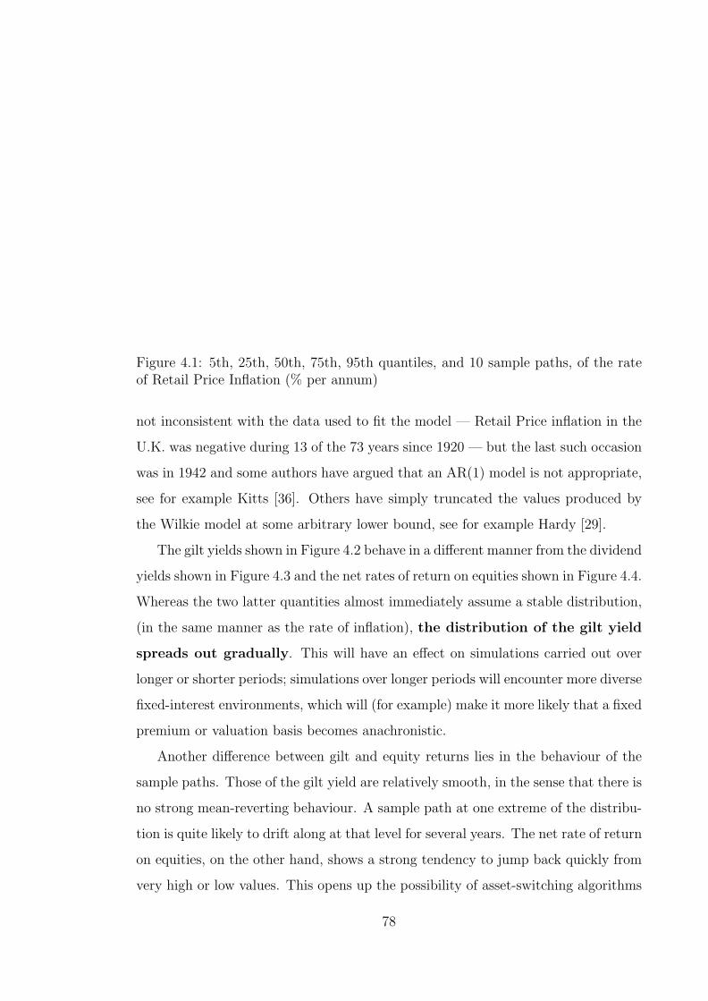
Figure 4.1: 5th, 25th, 50th, 75th, 95th quantiles, and 10 sample paths, of the rateof Retail Price Inflation (% per annum)
not inconsistent with the data used to fit the model — Retail Price inflation in the
U.K. was negative during 13 of the 73 years since 1920 — but the last such occasion
was in 1942 and some authors have argued that an AR(1) model is not appropriate,
see for example Kitts [36]. Others have simply truncated the values produced by
the Wilkie model at some arbitrary lower bound, see for example Hardy [29].
The gilt yields shown in Figure 4.2 behave in a different manner from the dividend
yields shown in Figure 4.3 and the net rates of return on equities shown in Figure 4.4.
Whereas the two latter quantities almost immediately assume a stable distribution,
(in the same manner as the rate of inflation), the distribution of the gilt yield
spreads out gradually. This will have an effect on simulations carried out over
longer or shorter periods; simulations over longer periods will encounter more diverse
fixed-interest environments, which will (for example) make it more likely that a fixed
premium or valuation basis becomes anachronistic.
Another difference between gilt and equity returns lies in the behaviour of the
sample paths. Those of the gilt yield are relatively smooth, in the sense that there is
no strong mean-reverting behaviour. A sample path at one extreme of the distribu-
tion is quite likely to drift along at that level for several years. The net rate of return
on equities, on the other hand, shows a strong tendency to jump back quickly from
very high or low values. This opens up the possibility of asset-switching algorithms
78

Figure 4.2: 5th, 25th, 50th, 75th, 95th quantiles, and 10 sample paths, of the netredemption yield on gilts (% per annum)
40 45 50 55 60 65 70
02
4
Figure 4.3: 5th, 25th, 50th, 75th, 95th quantiles, and 10 sample paths, of the netdividend yield (% per annum)
79
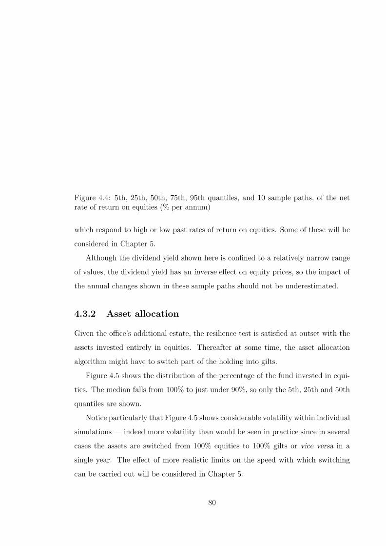
Figure 4.4: 5th, 25th, 50th, 75th, 95th quantiles, and 10 sample paths, of the netrate of return on equities (% per annum)
which respond to high or low past rates of return on equities. Some of these will be
considered in Chapter 5.
Although the dividend yield shown here is confined to a relatively narrow range
of values, the dividend yield has an inverse effect on equity prices, so the impact of
the annual changes shown in these sample paths should not be underestimated.
4.3.2 Asset allocation
Given the office’s additional estate, the resilience test is satisfied at outset with the
assets invested entirely in equities. Thereafter at some time, the asset allocation
algorithm might have to switch part of the holding into gilts.
Figure 4.5 shows the distribution of the percentage of the fund invested in equi-
ties. The median falls from 100% to just under 90%, so only the 5th, 25th and 50th
quantiles are shown.
Notice particularly that Figure 4.5 shows considerable volatility within individual
simulations — indeed more volatility than would be seen in practice since in several
cases the assets are switched from 100% equities to 100% gilts or vice versa in a
single year. The effect of more realistic limits on the speed with which switching
can be carried out will be considered in Chapter 5.
80
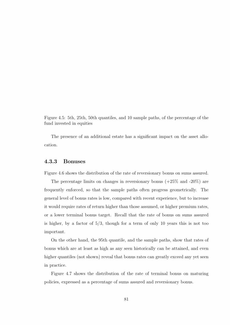
Figure 4.5: 5th, 25th, 50th quantiles, and 10 sample paths, of the percentage of thefund invested in equities
The presence of an additional estate has a significant impact on the asset allo-
cation.
4.3.3 Bonuses
Figure 4.6 shows the distribution of the rate of reversionary bonus on sums assured.
The percentage limits on changes in reversionary bonus (+25% and -20%) are
frequently enforced, so that the sample paths often progress geometrically. The
general level of bonus rates is low, compared with recent experience, but to increase
it would require rates of return higher than those assumed, or higher premium rates,
or a lower terminal bonus target. Recall that the rate of bonus on sums assured
is higher, by a factor of 5/3, though for a term of only 10 years this is not too
important.
On the other hand, the 95th quantile, and the sample paths, show that rates of
bonus which are at least as high as any seen historically can be attained, and even
higher quantiles (not shown) reveal that bonus rates can greatly exceed any yet seen
in practice.
Figure 4.7 shows the distribution of the rate of terminal bonus on maturing
policies, expressed as a percentage of sums assured and reversionary bonus.
81

Figure 4.6: 5th, 25th, 50th, 75th, 95th quantiles, and 10 sample paths, of the rateof reversionary bonus on sums assured (%)
40 45 50 55 60 65 70
-50
050
100
150
2
Figure 4.7: 5th, 25th, 50th, 75th, 95th quantiles, and 10 sample paths, of the rateof terminal bonus (% of sums assured + reversionary bonus)
82

The figure shows “negative” terminal bonuses. This is merely to indicate the
magnitude of the losses in any years when the guarantees exceed the available asset
shares. In this case the deficit, expressed as a percentage of the sum assured and
reversionary bonuses, is treated as a “theoretical” terminal bonus, but the rate of
terminal bonus actually declared is nil. It is interesting to consider the accumulated
amount of these losses, and ways of defraying that cost. In Chapter 6 we will return
to this question.
There is considerable volatility in terminal bonus. No attempt has been made at
this stage to smooth the emerging benefits or terminal bonus rates, but some of the
changes shown here are larger than past experience suggests would be acceptable.
This too will be considered in Chapter 6.
The terminal bonus emerging under deterministic conditions is consistently higher
than the target of 25%. This is because the reversionary bonuses are based on projec-
tions of asset shares and future premiums at the net gilt redemption yield, whereas
the fund is invested in equities and earns a higher net rate of return. The median
rate of terminal bonus is closer to 25% because the fund is more often invested in
gilts in the stochastic projections.
The effect of the reversionary and terminal bonuses combined on maturity values
is shown in Figure 4.8. This shows, not the maturity values per policy, (because
the average premium is inflation-linked) but the maturity values per unit premium.
This means that the figures in different years are directly comparable, either in the
absence of expenses as here, or if the expenses are linked to the same inflation index
as the average premium.
Apart from scale, this bears a strong resemblance to Figure 4.7. Terminal bonus
plays the greater part in the volatility of the overall results.
4.3.4 Financial ratios
Figure 4.9 shows the distribution of the ratio A/L1, measuring statutory solvency.
At any time, a small number of offices have a ratio A/L1 < 1, and are therefore
statutorily insolvent. Generally, recovery follows after a short period. However, the
small proportion of offices for which A/L1 < 1 at a single time hides the fact that
83

Figure 4.8: 5th, 25th, 50th, 75th, 95th quantiles, and 10 sample paths, of thematurity value per unit of annual premium
40 45 50 55 60 65 70
01
2
Figure 4.9: 5th, 25th, 50th, 75th, 95th quantiles, and 10 sample paths, of the ratioA/L1
84

Figure 4.10: Cumulative proportion of simulations (of 1,000) during which the ratioA/L1 has ever fallen below 1.1 (top), 1.05 (middle) or 1.0 (bottom)
different offices are statutorily insolvent at different times. Therefore,
the proportion of offices which are ever insolvent is much higher. Figure
4.10 shows the cumulative proportion, over time, of simulations in which the ratio
A/L1 has fallen below 1.1, 1.05 and 1.0 at least once.
Of the 1,000 simulations, 276 result in statutory insolvency at some
time. Moreover, 540 result in a ratio A/L1 of 1.05 or below at some time, which is
close to the level at which the E.C. solvency margins could not be covered (recall
that the ratio A/L1 excludes the E.C. solvency margin from the denominator).
Figure 4.11 shows the distribution of the ratio A/AS. The two influences on this
ratio are:
1. The cost of meeting the guarantees, when guaranteed maturity benefits exceed
asset shares at maturity.
2. The difference between the rate of new business growth and the rate of return
earned on the additional estate, which together decide the relative magnitude
of the additional estate, and hence the ratio A/AS. This will be touched upon
in Chapter 6.
In this case, the mean rate of new business growth is below the mean rate of
return on the assets, so the ratio A/AS ought to increase on the whole. Figure 4.11
85

Figure 4.11: 5th, 25th, 50th, 75th, 95th quantiles, and 10 sample paths, of the ratioA/AS
shows that the deterministic “skeleton” rises as expected, but the median in fact
falls (from 1.20 to about 1.09). This is an example, not uncommon, of determinism
leading to a conclusion which fails to capture some important characteristic.
The scale of Figure 4.11 is perhaps not ideal for revealing the detail of the sample
paths of the ratio A/AS, but it is the same scale as that of Figure 4.9, and it shows
interesting differences between the behaviour of the two ratios. The ratio A/L1 is
much more volatile; indeed the ratio A/AS has extremely smooth sample paths.
This difference has a bearing on their usefulness as criteria of financial strength,
which will be mentioned in Chapter 7.
The ratio A/AS will also be affected by any smoothing of maturity values, or
any attempt to charge for guarantees.
4.4 Discussion
4.4.1 Questions concerning strategies
The results presented here raise a number of questions, some of which will be ex-
plored in this and subsequent chapters.
1. The number of statutory insolvencies is relatively high, despite the use of
86

an asset allocation algorithm which is driven by statutory solvency. In part
this might be due to the use of 10-year policies, but Ross & McWhirter [58]
obtained comparable rates of statutory insolvency using a model with policies
of terms 5 years to 40 years. Therefore we might ask what gives rise to so
many insolvencies, and whether the asset allocation strategy is “shutting the
door after the horse has bolted”. This question will be addressed later in this
chapter.
2. The solvency-driven asset allocation algorithm is needed because the office
invests in equities; the office invests in equities because this gives the best
long-term results for policyholders; is this reasoning sound? It is a strongly
held view, especially in the U.K., but it rests partly on the assumption of an
inflationary economy. Part of the high returns associated with equities — or
more accurately, the inclusion of very high values in the distribution of equity
returns — can be ascribed to the tendency of equity dividends to move in line
with price indices over the long term. See, for example, Pentikainen et al [52].
The Wilkie model, although it allows for a moderately inflationary economy in
the long run, also allows for considerable periods of low or negative inflation.
Under these circumstances, is there any reason to assume that equities will
produce better maturity values than gilts?
It is worth investigating the real maturity values, allowing for the loss (or gain!)
in purchasing power during the policy term. This will be done in Chapter 5.
3. The assumption of a fixed proportion in equities, possibly subject to solvency-
led constraints, is not the only plausible assumption. There might be switching
opportunities within the Wilkie model. This is also investigated in Chapter 5.
4. The solvency-driven asset allocation strategy used here, which is similar to that
of Ross [57], results in some reduction in the incidence of statutory insolvency
(looking ahead to Chapter 5), but at the expense of very large asset switches.
Assuming that asset switching is subject to more realistic market constraints,
is the strategy still effective? This is investigated briefly in Chapter 5.
5. The emerging reversionary bonus rates often appear “unrealistically” low or
87

high, even although the changes in reversionary bonus rates are constrained.
Since bonus declarations add to the guarantees, the nature of these constraints
could have a considerable effect on solvency. The effect could be either way,
since there might be as much reluctance to reduce bonus rates, for commer-
cial reasons, as to increase them. Different reversionary bonus strategies and
constraints are considered briefly in Chapter 5, and will also be touched upon
in Chapter 6.
6. Maturity values, and terminal bonus rates, appear more volatile than past
history would suggest they should be. This arises from the simple treatment
of with-profits business in the model, as unit-linked business with a managed
fund and a guarantee. A more realistic treatment would include the smoothing
of maturity values. This is the topic of Chapter 6.
In most of these cases it is necessary to guess what actions managers might take if
faced with conditions quite unlike any experienced in the past. For example, an un-
precedented bull market in equities might result in (i) historically high reversionary
bonus rates, or (ii) historically high terminal bonus rates, or (iii) historically high
A/L ratios, or (iv) all of these. On the other hand, adverse conditions create dif-
ferent problems with which managements have not been faced before. It is perhaps
not reasonable to reject an algorithm because it leads to an unprecedented result in
unprecedented conditions. Rather such a result suggests strengths or weaknesses of
the algorithms considered.
4.4.2 Questions concerning solvency
Wider questions which we will consider concern the nature of solvency, and the
effectiveness of a traditional solvency valuation. These are the topics of Chapter
7 and Chapter 8. The subject area has already been introduced in Chapter 2 and
Chapter 3.
1. How closely does “insolvency” under any traditional solvency valuation corre-
spond to a deficit in the run-off?
88

2. What is the role of each part of the system in determining statutory solvency
— valuation regulations, E.C. solvency margins, resilience test?
3. What would be the effect of different valuation regimes, such as those typical
of other E.C. territories or North America?
In the remainder of this chapter we use the simple model described above to
examine, as far as they can be discerned, some factors which might be associated
with statutory insolvency. It is important to emphasise the strong dependence of
these and subsequent explorations on the assumptions used in the model, and the
structure and parameters of the underlying Wilkie asset model.
4.5 Statutory insolvency in the model
4.5.1 The general pattern of statutory insolvency
The first question to ask is whether statutory insolvency is associated with particular
patterns of financial conditions or bonus declarations.
The 1,000 simulations described above included 276 in which statutory solvency
ever occurred — that is, in which the ratio A/L1 fell below 1.0 at some time. Figure
4.12 shows the ratio A/L1 (sorted in ascending order) upon the first such failure in
each of these 276 simulations.
There are comparatively few “catastrophic” failures, and many more “moderate”
failures. In about half of the cases the ratio A/L1 on first insolvency lies between
0.95 and 1.0.
Figure 4.13 shows the distribution of times at which statutory insolvency first
occurs, for the 276 cases in which it does occur. There is a slight downward trend.
However, if we plot the rate at which statutory insolvencies first occur
No. of new insolvencies at time t
No. of offices never insolvent before time t
(an empirical estimate of the “mortality rate” of these offices) which is shown in
Figure 4.14, there is no obvious trend in the rate at which still-solvent offices fail.
89

Figure 4.12: Ratio A/L1 of the 276 statutory insolvencies on first failure (sorted)
40 45 50 55 60 65 70
05
10
Figure 4.13: Distribution of times at which statutory insolvency first occurs
90

Figure 4.14: Rate of occurrence of new statutory insolvencies
4.5.2 Conditions leading to statutory insolvency
Hardy [29] carried out 1,000 simulations of a model office and studied those 100
cases in which the ratio A/L1 attained its lowest values (about 1.04 or below). An
interesting feature of these simulations was a tendency to exhibit low inflation in
the earlier years of the projection period. Hardy said
“Despite the fact that expenses are linked to inflation, and that after
the 5th year there is no new business, it is low inflation, not high infla-
tion, that causes the greater insolvency risk, because of the association
between inflation and equity returns.”
How direct is the association between low inflation and statutory insolvency in
our model? There is not likely to be low inflation throughout the 30-year projection
period in any one simulation — this would be surprising given that an AR(1) process
is used to model inflation — so there is little point in looking at distributions like
those in Figure 4.1. Of more potential interest is the distribution of the rate of RPI
at the time when insolvency occurs.
Figure 4.15 shows the “distribution” of the rate of Retail Price Inflation in all 276
simulations in which statutory insolvency occurred, during the 10 years before and
after statutory insolvency first occurred. The timescale runs from −10 years (i.e.
91

Figure 4.15: 5th, 25th, 50th, 75th, 95th quantiles, and 10 sample paths, of the rateof Retail Price Inflation (in 10 years around A/L1 < 1)
10 years before insolvency) to +10 years (i.e. 10 years after insolvency). The word
“distribution” above is placed in inverted commas because by comparing sample
paths at different times, we are no longer looking at sample paths drawn from a
common distribution, but simply looking for similarities between certain parts of
different sample paths.
Here we are mainly interested in the conditions which precede statutory in-
solvency, but in Chapter 7 we will also be interested in the conditions following
insolvency, so these figures show both.
Note that not all of these “sample paths” are complete, since some insolvencies
occur in the first and last 10 years of the projection period. The “quantiles” are
based on the number of simulations actually included at each time before or after
insolvency.
There is evidence in the quantile plots of
1. a downward drift of inflation in the years preceding insolvency, and
2. a rise in inflation back to “normal” levels at the time of insolvency.
Some caution is needed in assessing these “features” — they are clear from the
quantile plots, but not at all clear from the sample paths. (Only 10 paths are shown
92

Figure 4.16: 5th, 25th, 50th, 75th, 95th quantiles, and 10 sample paths, of the ratioA/L1 (in 10 years around RPI <-10%)
here, but it is still true of larger samples.) Not all sample paths of inflation drift
down and then rise just before insolvency; some do the opposite. Low
inflation in terms of the distribution cannot be sufficient causal explanation.
Figure 4.16 looks at this from another angle. Instead of showing the RPI in the
years around a fall in the ratio A/L1 to 1.0 or below, it shows the ratio A/L1 in
the 10 years before and after the rate of RPI falls below −10% for the first time.
Inflation as low as −10% occurs in 122 of the 1,000 simulations.
There is some evidence of a reduction in the ratio A/L1 following such severe
deflation. However, only in 50 out of the 122 simulations in which the RPI reached
−10% did insolvency also occur.
4.5.3 The mechanism of failure
The previous section described some evidence that low inflation influences insol-
vency. However this does not explain why insolvencies occur at some times and
not at others. An unconvincing aspect of the “evidence” is the inconsistency of the
sample paths of the rate of RPI. Individual failures are not caused by median rates
of RPI. In looking for a mechanism of failures, the evidence of quantiles or means
is insufficient — we are looking for some property of the sample paths.
93

Figure 4.17: 5th, 25th, 50th, 75th, 95th quantiles, and 10 sample paths, of the netdividend yield (in 10 years around A/L1 < 1)
Figure 4.17 shows the “distribution” of the net dividend yields, and Figure 4.18
shows the “distribution” of the net rate of return on equities, in the 10 years before
and after the first occurrence of statutory insolvency.
These figures suggest a link between insolvencies and stock market
crashes, which are themselves associated with increases in the dividend
yield. Moreover, this is a feature displayed by the sample paths as well
as the quantiles.
Figure 4.18 suggests that the net rate of return on equities is slightly low in
the year preceding insolvency, but not in any earlier years. It is possible that low
inflation plays a part in this. However, since we know how the Wilkie model works,
we can calculate the relative effect of inflation on the factors leading to equity price
falls.
The Wilkie model generates an index of dividends D(t) and a dividend yield
Y (t). Therefore the change in equity prices is given by
D(t)
D(t− 1)
Y (t− 1)
Y (t)
Inflation has only a mild effect on the index of dividends. Recall that the index
of dividends is given by
94

Figure 4.18: 5th, 25th, 50th, 75th, 95th quantiles, and 10 sample paths, of the netrate of return on equities (in 10 years around A/L1 < 1)
log
(D(t)
D(t− 1)
)= 0.8DM(t) + 0.2 log
(Q(t)
Q(t− 1)
)− 0.0525Y Z(t− 1) + 0.1DZ(t)
where
DM(t) = 0.2 log
(Q(t)
Q(t− 1)
)+ 0.8DM(t− 1)
so that
(D(t)
D(t− 1)
)∝
(Q(t)
Q(t− 1)
)0.36
That is, the change in dividends is in proportion to a small power of Q(t)Q(t−1)
, if
we ignore the exponentially lagged influence of previous inflation in DM(t). On the
other hand
(D(t)
D(t− 1)
)∝ e0.1DZ(t)
and {DZ(t)} is a sequence of i.i.d. Normal(0,1) random variables. Figure 4.19
shows the relative influences of the inflation component and the white noise com-
ponent on the change in the dividend index, based on a single simulation over 100
years. The solid line shows
e0.1DZ(t) = 1.105DZ(t)
95

Figure 4.19: Effect of white noise terms (solid line) and inflation terms (dotted line)on D(t)/D(t− 1) during 100 years
and the dotted line shows
(Q(t)
Q(t− 1)
)0.36
Now recall that the dividend yield Y (t) is given by
log(Y (t)) = 1.35 log
(Q(t)
Q(t− 1)
)+ Y N(t)
where
Y N(t) = log 0.04 + 0.6{Y N(t− 1)− log 0.04}+ 0.175Y Z(t)
so that
Y (t) ∝(
Q(t)
Q(t− 1)
)1.35
and
(Y (t)
Y (t− 1)
)∝
(Q(t)Q(t− 2)
Q(t− 1)2
)1.35
But also
(Y (t)
Y (t− 1)
)∝ e0.175(Y Z(t)−Y Z(t−1)) = 1.19Y Z(t)−Y Z(t−1)
Where the {Y Z(t)} are i.i.d. Normal(0,1) random variables.
96

Figure 4.20: Effect of white noise terms (solid line) and inflation terms (dotted line)on Y (t)/Y (t− 1) during 100 years
Figure 4.20 shows the relative influences of the inflation component and the white
noise component on the change in dividend yields, based on a single simulation over
100 years. The solid line shows
1.19Y Z(t)−Y Z(t−1)
and the dotted line shows (Q(t)Q(t− 2)
Q(t− 1)2
)1.35
The white noise terms have a greater effect than inflation on both
components of the change in equity prices. This might answer the question:
why is low inflation not a strong feature of the sample paths in the “low inflation”
insolvencies?
Figure 4.21 shows the proportion of the funds invested in equities in the 10 years
before and after statutory insolvency. (The bottom quantile shown before insolvency
is, in fact, the 5th quantile — this might not be obvious in the Figure.) Therefore
75% of offices are invested 80% or more in equities, and almost 50% are invested
100% in equities, at the time of insolvency. This is higher than the average for all
offices (see Figure 4.5), again consistent with a pattern of insolvencies linked to falls
in equity prices.
97

Figure 4.21: 5th, 25th, 50th, 75th, 95th quantiles, and 10 sample paths, of the % ofthe fund in equities (in 10 years around A/L1 < 1)
For completeness, Figure 4.22 shows the “distribution” of the net gilt redemption
yield in the 10 years before and after statutory insolvency. The evidence of low, or
even unusually distributed, gilt yields is slight.
4.5.4 More experiments with inflation
To test further the influence of inflation on statutory insolvency, we can try the
simple experiment of using constant inflation in the model. That is, the 1,000
simulations were re-run with the standard deviation QSD set to 0 in the Wilkie
inflation model. The rate of inflation was therefore a constant 5.127%, with the
other white noise components DSD, Y SD and CSD as before.
The number of statutory insolvencies fell from 276 to 184. There were 130
scenarios in which statutory insolvency occurred in both cases. There were therefore
146 scenarios in which statutory insolvency occurred with QSD = 0.05, but not with
QSD = 0. This is not evidence for the influence of low inflation, merely evidence
that the variability induced by QSD makes insolvency more likely.
For convenience, refer to the 130 scenarios in which insolvency still occurred
with QSD = 0 as “Group A” scenarios, and the other 146 in which insolvency only
occurred when QSD = 0.05 as “Group B” scenarios.
98

Figure 4.22: 5th, 25th, 50th, 75th, 95th quantiles, and 10 sample paths, of net giltredemption yield (in 10 years around A/L1 < 1)
Consider Group A. Changing the rate of inflation will change the other elements
of the asset model, and it is not obvious that the sample paths of the yields and
prices should be at all similar. In particular, it is not obvious that insolvency, though
it occurs in both cases, should occur at the same times in each of the 130 scenarios,
and from the same causes. Figure 4.23 shows the difference of the times at which
statutory insolvency first occurs in each scenarios, in other words
Time of insolvency with QSD = 0.05− Time of insolvency with QSD = 0
All but a few insolvencies do in fact occur at the same times with QSD = 0.05
and with QSD = 0, suggesting that low inflation up to and including the time of
insolvency does not play too important a part in these cases — nearly half of all the
insolvencies.
Still considering the Group A simulations Figure 4.24 shows the “distribution” of
the rate of RPI in the 10 years around statutory insolvency for these 130 simulations.
Note carefully that these simulations are made with QSD = 0.05, but they are the
130 cases in which insolvency still occurred with QSD = 0.
This shows little evidence of low inflation before insolvency. However, Figure
4.25 shows the “distribution” of the rate of RPI in the 10 years around statutory
insolvency for the 146 Group B simulations, in which insolvency did not occur with
99

Figure 4.23: Time of insolvency with QSD = 0.05 minus time of insolvency withQSD = 0
-10 -5 0 5 10
-20
-10
010
20
Figure 4.24: 5th, 25th, 50th, 75th, 95th quantiles, and 10 sample paths, of rate ofRPI (in 10 years around A/L1 < 1) in those scenarios insolvent if QSD = 0
100

Figure 4.25: 5th, 25th, 50th, 75th, 95th quantiles, and 10 sample paths, of rate ofRPI (in 10 years around A/L1 < 1) solvent if QSD = 0
QSD = 0 but did occur with QSD = 0.05.
There is a more marked tendency for inflation to be low before insolvency occurs
— indeed more marked even than in Figure 4.15. Once again, the rise in inflation
at the time of insolvency is a feature.
Re-running the 1,000 simulations with QSD = 0.05, but eliminating the the
white noise component of the dividend yield by setting Y SD = 0 had the following
result: the number of insolvencies fell from 276 to 11, and of these 11, 6 were also
among the original 276 and 5 were not.
Re-running the 1,000 simulations with the white noise of the dividend index
DSD set to zero resulted in 175 insolvencies, 113 of which were also among the
original 276 simulations.
Re-running the 1,000 simulations with the white noise component of the consols
yield CSD set to zero had a negligible effect, owing to (i) the predominance of equity
investment, and (ii) the absence of statutory insolvencies at times when there is any
degree of investment in gilts. This last point will become clearer in Chapter 5;
note however that it is not to be confused with the fact that there must be 100%
investment in gilts just after insolvency has occurred.
101

4.5.5 Conclusions
1. Statutory insolvency, in this model, is strongly associated with catastrophic
falls in share prices. This association is a property of the sample paths.
2. Falls in share prices are influenced largely by the white noise components of the
dividend yield model and dividend index models. Inflation is a lesser influence.
3. Low inflation is associated with some but not all statutory insolvencies.
4. Offices which suffer statutory insolvency tend to be slightly more heavily in-
vested in equities than average when the insolvency occurs.
102

Chapter 5
The impact of different strategies
5.1 Introduction
The managers of a with-profit life office can attempt, within the constraints imposed
by regulations, to control the financial position of that office by their decisions in
respect of
1. asset allocation,
2. the granting of guarantees (premium setting and/or bonuses)
3. the smoothing of benefits
Each of the factors above may be both an input and an output at the same
time. Management might have a preferred strategy for each, in which sense they
are inputs. The interactions between them (and the regulations) might lead to
departures from the preferred strategy, in which sense they are outputs.
This chapter examines the influence of the office’s asset allocation and reversion-
ary bonus strategies on statutory solvency and policyholder’s benefits. The effect of
a given strategy may be gauged by comparing the distributions of suitable outputs
with some “baseline” set of projections, such as those illustrated in Chapter 4.
103

5.2 Summary statistics
While graphs help us to understand the general behaviour of the sample paths in
a stochastic model office, they are less suitable for comparing large sets of alterna-
tive projections. As with single-figure mortality indices, it is useful to have some
summary statistics.
We may wish to compare:
1. variability within individual scenarios, and
2. variability between different scenarios.
Given a quantity X it defined at each time t = 1, . . . , n within each scenario
i = 1, . . . ,m, define the following (sample) means:
Et(Xit) =
1
n
t=n∑t=1
X it
Ei(X it) =
1
m
i=m∑i=1
X it
Eit(X
it) = Ei(Et(X
it))
= Et(Ei(X i
t))
Within each scenario the simplest measures of the behaviour of X it are its max-
imum, maxt(Xit), minimum, mint(X
it), mean, Et(X
it) and standard deviation, de-
noted St(Xit) where the subscript t indicates that the extrema or moments are
calculated with respect to time.
Then some suitable statistics are these:
Distribution of Et(Xit). We summarise the distribution of Et(X
it) by its mean and
standard deviation over the 1,000 scenarios, denoted by Eit(X
it) and Si(Et(X
it))
respectively.
Mean of St(Xit). The quantity Si(Et(X
it)) sums up the range of variation between
different scenarios. If we reverse the order of the operations, and denote by
Ei(St(Xit)) the mean across all 1,000 scenarios of St(X
it), this will measure
variability within scenarios.
104

Distribution of maxt(Xit). The mean and standard deviation of maxt(X
it) will be
denoted Ei(maxt(Xit)) and Si(maxt(X
it)). A large standard deviation indicates
a wide range of extremes within the 1,000 scenarios, which in turn indicates
that problems, if any, will lie with a small number of “exceptional” scenarios
which might repay study. A low value, on the other hand, suggests more
homogeneous behaviour of the sample paths.
Distribution of mint(Xit). The mean and standard deviation of mint(X
it) will be
denoted Ei(mint(Xit)) and Si(mint(X
it)).
Correlations. Coefficients of correlation will be introduced as required, and will
be denoted by C(, ). Note that we can either (i) calculate the correlation
between two quantities X it and Y i
t within each simulation, denoted Ct(Xit , Y
it ),
and then calculate its moments across all the scenarios, Ei(Ct(Xit , Y
it )) etc.,
or (ii) calculate moments or other statistics within each scenario, for example
mint(Xit) and Et(Y
it ), and then compute the correlation Ci(mint(X
it), Et(Y
it )).
There is an example of this in Table 5.10, where X is the ratio A/L1 and Y is
the maturity value per unit premium.
5.3 Fixed asset allocation strategies
The baseline model of Chapter 4 uses a dynamic asset allocation strategy driven
by statutory solvency, similar to those of Ross [57] and Ross & McWhirter [58].
These authors compared the outcomes with fixed asset allocation strategies (80% in
equities) and drew unfavourable conclusions about the effects on payouts to policy-
holders of the dynamic strategy.
In this section we compare different fixed asset allocation strategies with the
solvency-driven dynamic asset allocation strategy. Table 5.9 defines 11 fixed strate-
gies, ranging from 100% in equities to 0% in equities. In each case the balance of
the fund is invested in gilts.
105

Strategy % of Assets In-vested in Equities
AA No.1 100%AA No.2 90%AA No.3 80%AA No.4 70%AA No.5 60%AA No.6 50%AA No.7 40%AA No.8 30%AA No.9 20%AA No.10 10%AA No.11 0%
Table 5.9: Definition of Asset Allocation Strategies AA No.1 – AA No.11
5.3.1 The trade-off between solvency and high returns
It is normally assumed that investment in equities brings the prospect of high returns
(represented here by the maturity values) but at the expense of both greater variance
of the returns and a greater risk of insolvency. Evidence for this has been found in
simulation studies (see, for example, Forfar et. al. [22]). Investment in gilts, on the
other hand, is held to be safer but with reduced prospects.
Table 5.10 shows, for the 11 strategies defined above, the numbers of statu-
tory insolvencies, and some summary statistics in respect of the ratio A/L1 and the
maturity value (MV) per unit premium. The last column headed “Corr” requires ex-
planation. It shows the correlation between mint(A/L1) and Et(MV it ); that is, both
of these are calculated in respect of each scenario, and the correlation is calculated
from the resulting 1,000 pairs.
The table shows the following features as the proportion invested in equities falls:
1. The number of statutory insolvencies falls steeply, and the distribution
of the minimum A/L1 ratio attained in each scenario becomes much more
concentrated. Figure 5.26 shows estimates of the densities of the ratio A/L1
at time t = 70 with 100%, 50% and 0% in equities, and Figure 5.27 shows how
the distribution of the ratio A/L1 evolves over time with 100% in equities.
2. Equity investment results in a distribution of maturity values with
106

Ratio A/L1 MV per unit prem.
Strategy No. < 1 Ei(mint) Si(mint) Eit Si(Et) Ei(St) Corr
AA No.1 745 0.808 0.284 18.218 2.871 5.449 0.178AA No.2 624 0.893 0.236 17.846 2.579 4.877 0.186AA No.3 485 0.976 0.194 17.467 2.299 4.327 0.197AA No.4 321 1.054 0.159 17.091 2.037 3.791 0.187AA No.5 156 1.128 0.127 16.718 1.794 3.271 0.172AA No.6 42 1.198 0.100 16.356 1.571 2.761 0.142AA No.7 2 1.265 0.074 16.005 1.368 2.263 0.093AA No.8 0 1.328 0.055 15.668 1.187 1.779 0.026AA No.9 0 1.387 0.040 15.344 1.033 1.330 −0.063AA No.10 0 1.442 0.031 15.020 0.916 0.977 −0.193AA No.11 0 1.478 0.029 14.694 0.846 0.845 −0.217
Table 5.10: Comparison of ratio A/L1 with Maturity Values, strategies AA No.1 –AA No.11 (fixed investment strategies).
0 2 4 6
01
2
Figure 5.26: Estimates of the density of the ratio A/L1 at time t = 70 with 100%,50% and 0% equity investment.
107
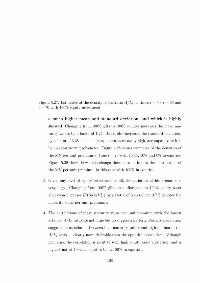
Figure 5.27: Estimates of the density of the ratio A/L1 at times t = 50, t = 60 andt = 70 with 100% equity investment.
a much higher mean and standard deviation, and which is highly
skewed. Changing from 100% gilts to 100% equities increases the mean ma-
turity values by a factor of 1.24. But it also increases the standard deviation,
by a factor of 3.38. This might appear unacceptably high, accompanied as it is
by 745 statutory insolvencies. Figure 5.28 shows estimates of the densities of
the MV per unit premium at time t = 70 with 100%, 50% and 0% in equities.
Figure 5.29 shows how little change there is over time in the distribution of
the MV per unit premium, in this case with 100% in equities.
3. Given any level of equity investment at all, the variation within scenarios is
very high. Changing from 100% gilt asset allocation to 100% equity asset
allocation increases Ei(St(MV it)) by a factor of 6.45 (where MV i
t denotes the
maturity value per unit premium).
4. The correlations of mean maturity value per unit premium with the lowest
attained A/L1 ratio are not large but do suggest a pattern. Positive correlation
suggests an association between high maturity values and high minima of the
A/L1 ratio — clearly more desirable than the opposite association. Although
not large, the correlation is positive with high equity asset allocation, and is
highest not at 100% in equities but at 80% in equities.
108

Figure 5.28: Estimates of the density of the MV per unit premium at time t = 70with 100%, 50% and 0% equity investment.
0 20 40 60 80
0.0
0.05
0.10
0.15
Figure 5.29: Estimates of the density of the MV per unit premium at times t = 50,t = 60 and t = 70 with 100% equity investment.
109

Figure 5.30: Boxplot of ratio A/L1 at time t = 70 under asset allocation strategiesAA No.1 – AA No.11.
A convenient tool for comparing several distributions is the boxplot. For exam-
ple, Figure 5.30 shows box-plots of the ratio A/L1 at time t = 70.
The components of a box plot are (i) the box, (ii) the whiskers and (iii) the
outliers.
1. The shaded box indicates the quartiles of the distribution. It is bounded above
and below by the upper and lower quartiles respectively.
2. The white line in the box shows the location of the median.
3. The dotted lines extending above and below the box indicate, on each side,
1.5 × the inter-quartile range. If, however, the furthest observation on one or
other side lies closer to the nearest quartile than 1.5 × the inter-quartile range,
the dotted line and its terminating whisker will be truncated accordingly.
4. The horizontal lines beyond the whiskers indicate observations beyond the
range of the whiskers. If they are clustered thickly on one side but not the
other (as in this figure) this indicates skewness.
Using a box plot it is relatively easy to compare by eye the distributions under
different assumptions. The disadvantage is that when comparing time-series data
under different assumptions, the box plot can only show a “snapshot” at a single
110

Figure 5.31: Boxplot of the MV per unit premium at time t = 70 under assetallocation strategies AA No.1 – AA No.11.
time. In terms of the summary statistics above, it illustrates the “between scenario”
variability at a given time, but not how it evolves over time.
Note that the vertical scales in this (and all other) box plots shown here are
chosen to be the same as the scales used for quantile plots such as those in Chapter
4. This means that extreme outliers will sometimes be omitted from the plot. On
the other hand, choosing a scale which includes all outliers would usually compress
all but the extreme quantiles into an indistinguishable band. Using a uniform scale
has the advantage that comparisons can be made by eye, and this is worth the loss
of a few outliers.
Figure 5.31 shows a boxplot of the MVs per unit premium at time t = 70 under
the strategies AA No.1 – AA No.11. Both the increased variance and skewness
associated with equity investment are evident. Note also that there is much less
difference between the medians and the lower quantiles.
5.3.2 The trade-off between solvency and real returns
Since rates of return in the Wilkie asset model are positively correlated with rates
of inflation, high maturity values will to some extent reflect high inflation, and low
maturity values, low inflation. We might obtain a more consistent comparison of
111

Ratio A/L1 Real MV per unit prem.
Strategy No. < 1 Ei(mint) Si(mint) Eit Si(Et) Ei(St) Corr
AA No.1 745 0.808 0.284 11.032 1.732 3.399 −0.109AA No.2 624 0.893 0.236 10.840 1.645 3.167 −0.073AA No.3 485 0.976 0.194 10.641 1.570 2.951 −0.034AA No.4 321 1.054 0.159 10.443 1.507 2.754 0.000AA No.5 156 1.128 0.127 10.247 1.458 2.577 0.033AA No.6 42 1.198 0.100 10.057 1.420 2.423 0.077AA No.7 2 1.265 0.074 9.875 1.397 2.297 0.137AA No.8 0 1.328 0.055 9.703 1.391 2.209 0.207AA No.9 0 1.387 0.040 9.540 1.402 2.165 0.297AA No.10 0 1.442 0.031 9.379 1.430 2.171 0.417AA No.11 0 1.478 0.029 9.214 1.468 2.220 0.503
Table 5.11: Comparison of ratio A/L1 with real Maturity Values, strategies AANo.1 – AA No.11 (fixed investment strategies).
maturity values in real terms than in nominal terms.
Let RV it be the real maturity value per unit premium at time t in the ith scenario,
defined as
RV it =
MV it
Qit/Q
it−10
where Qit is the Retail Price Index at time t in the ith scenario. Table 5.11 shows
the same summary statistics as Table 5.10 in respect of RV it.
There are interesting differences between Tables 5.10 and 5.11.
1. Equity investment still yields higher maturity values; changing from 100% in
gilts to 100% in equities increases Eit(RV i
t) by a factor of 1.20, which is close
to the increase of 1.24 in nominal terms.
2. The distributions of real maturity values are quite similar, regardless
of the level of equity investment. Figure 5.32 shows estimates of the
densities of the real MV per unit premium at time t = 70 with 100%, 50% and
0% in equities. All are highly skew.
3. There is much less variability between scenarios; changing from 100%
in gilts to 100% in equities increases Si(Et(RV it)) by a factor of only 1.18,
instead of 3.38 in nominal terms.
112

Figure 5.32: Estimates of the density of the real MV per unit premium at timet = 70 with 100%, 50% and 0% equity investment.
4. Si(Et(RV it)) does not vary much below about 60% equity investment (AA
No.6). The minimum is at about 30% equity asset allocation (AA No.8).
There is not much reason to prefer any level of equity investment between 0%
and 60%, in terms of mean real maturity values.
5. The dependence of the “within scenarios” variability on the level of equity
investment is much reduced; moving from 100% in gilts to 100% in equities
increases Ei(St(RV it)) by a factor of 1.53, compared with an increase of 6.54
in Ei(St(MV it)).
6. Ei(St(RV it)) > Ei(St(MV i
t)) under high levels of gilt investment, despite the
fact that Eit(RV i
t) < Eit(MV i
t). This indicates that the variability within
scenarios is greater in real terms than in nominal terms.
7. The correlations between mint(A/L1) and Et(RV it) display a contrary trend
to those between mint(A/L1) and Et(MV it). In other words the association
between higher real maturity values and higher minima of the ratio A/L1 is
strongest under investment in gilts.
Figure 5.33 shows a boxplot of the real MVs per unit premium at time t = 70
under strategies AA No.1 – AA No.11.
113
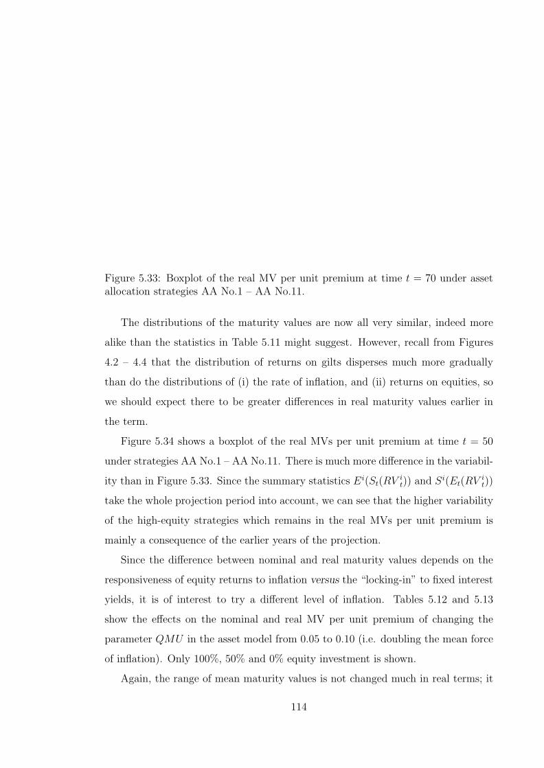
Figure 5.33: Boxplot of the real MV per unit premium at time t = 70 under assetallocation strategies AA No.1 – AA No.11.
The distributions of the maturity values are now all very similar, indeed more
alike than the statistics in Table 5.11 might suggest. However, recall from Figures
4.2 – 4.4 that the distribution of returns on gilts disperses much more gradually
than do the distributions of (i) the rate of inflation, and (ii) returns on equities, so
we should expect there to be greater differences in real maturity values earlier in
the term.
Figure 5.34 shows a boxplot of the real MVs per unit premium at time t = 50
under strategies AA No.1 – AA No.11. There is much more difference in the variabil-
ity than in Figure 5.33. Since the summary statistics Ei(St(RV it)) and Si(Et(RV i
t))
take the whole projection period into account, we can see that the higher variability
of the high-equity strategies which remains in the real MVs per unit premium is
mainly a consequence of the earlier years of the projection.
Since the difference between nominal and real maturity values depends on the
responsiveness of equity returns to inflation versus the “locking-in” to fixed interest
yields, it is of interest to try a different level of inflation. Tables 5.12 and 5.13
show the effects on the nominal and real MV per unit premium of changing the
parameter QMU in the asset model from 0.05 to 0.10 (i.e. doubling the mean force
of inflation). Only 100%, 50% and 0% equity investment is shown.
Again, the range of mean maturity values is not changed much in real terms; it
114

Figure 5.34: Boxplot of the real MV per unit premium at time t = 50 under assetallocation strategies AA No.1 – AA No.11.
Ratio A/L1 MV per unit prem.
Equity % No. < 1 Ei(mint) Si(mint) Eit Si(Et) Ei(St) Corr
100% 677 0.895 0.197 22.819 4.111 8.203 0.13250% 47 1.182 0.100 19.121 2.033 3.956 0.0850% 8 1.340 0.090 15.987 1.091 1.53 0.283
Table 5.12: Comparison of ratio A/L1 with Maturity Values, 100%, 50% and 0% inequities, QMU = 0.1 in the asset model.
Ratio A/L1 Real MV per unit prem.
Equity % No. < 1 Ei(mint) Si(mint) Eit Si(Et) Ei(St) Corr
100% 677 0.895 0.197 9.209 1.420 2.949 0.10250% 47 1.182 0.100 7.954 1.098 2.057 0.2750% 8 1.340 0.090 6.880 1.107 2.012 0.248
Table 5.13: Comparison of ratio A/L1 with real Maturity Values, 100%, 50% and0% in equities, QMU = 0.1 in the asset model.
115

falls from 1.42 to 1.33. But the variability, between and within scenarios, lies within
a much smaller range in real terms. In much more inflationary conditions, therefore,
the same conclusion is reached.
These results suggest that one part of the supposed penalty for in-
vesting in equities — more variable maturity values — is overstated if we
look at nominal and not real maturity values. That does not affect the other
part of the penalty — the very much higher incidence of insolvency. The question
of whether or not that too is overstated will be discussed in Chapter 7.
5.4 Declining EBR strategies
A method often suggested of obtaining exposure to equities while protecting ma-
turity guarantees is to employ a declining Equity Backing Ratio (EBR) (see, for
example, Kennedy et al [35] and Smaller [62]). This means that the assets under-
lying a policy’s asset share are progressively switched out of equities and into gilts
as maturity approaches. Under such a strategy, the overall split between gilts and
equities is not static, since it depends on the composition of the business, but the
strategy itself is static.
Following Smaller [62], Forfar et al [22] investigated a wide range of declining
EBR strategies, using a 20-year term. They said
“It will be seen that the effect of the falling EBR has been to reduce
the fluctuations of the asset share AS(20), as measured by the standard
deviation, but the smaller standard deviation has been achieved at the
expense of a smaller mean return.”
Six simple declining EBR strategies are considered here. They are described in
Table 5.14. Tables 5.15 and 5.16 show the summary statistics in respect of MV it
and RV it respectively.
These lead to very similar conclusions to those of Section 5.3. The mean maturity
values, comparing one strategy with another, are in a similar relationship in both
tables, but the large differences in variability as between one strategy and another
shown in Table 5.15 are almost eliminated in Table 5.16.
116

Strategy % of Assets Invested in Equities
AA No.12 100% until duration 5 years, 75% thereafterAA No.13 100% until duration 5 years, 50% thereafterAA No.14 100% until duration 5 years, 25% thereafterAA No.15 100% until duration 5 years, 0% thereafterAA No.16 100% until duration 5 years, falling linearly to 0% at maturityAA No.17 100% at inception, falling linearly to 0% at maturity
Table 5.14: Definition of Asset Allocation Strategies AA No.12 – AA No.17
Ratio A/L1 MV per unit prem.
Strategy No. < 1 Ei(mint) Si(mint) Eit Si(Et) Ei(St) Corr
AA No.12 534 0.954 0.202 17.522 2.398 4.263 0.170AA No.13 275 1.071 0.151 16.861 1.967 3.288 0.104AA No.14 103 1.159 0.126 16.260 1.589 2.678 −0.024AA No.15 39 1.212 0.119 15.738 1.295 2.611 −0.169AA No.16 392 1.017 0.165 16.986 2.117 3.517 0.083AA No.17 21 1.217 0.094 16.005 1.454 2.149 0.047
Table 5.15: Comparison of ratio A/L1 with Maturity Values, strategies AA No.12 –AA No.17 (declining EBRs).
Ratio A/L1 Real MV per unit prem.
Strategy No. < 1 Ei(mint) Si(mint) Eit Si(Et) Ei(St) Corr
AA No.12 534 0.954 0.202 10.670 1.588 2.918 −0.047AA No.13 275 1.071 0.151 10.330 1.487 2.597 0.004AA No.14 103 1.159 0.126 10.033 1.440 2.507 0.019AA No.15 39 1.212 0.119 9.789 1.465 2.673 −0.028AA No.16 392 1.017 0.165 10.395 1.527 2.682 −0.064AA No.17 21 1.217 0.094 9.885 1.406 2.311 0.097
Table 5.16: Comparison of ratio A/L1 with Real Maturity Values, strategies AANo.12 – AA No.17 (declining EBRs).
117
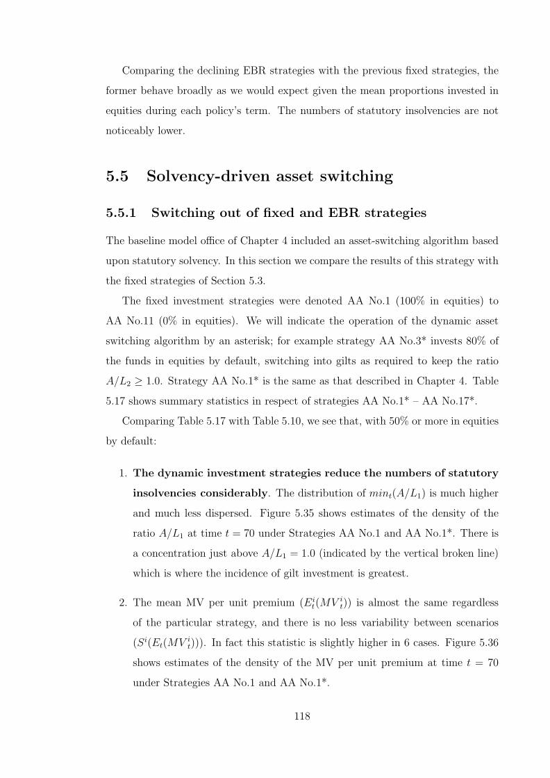
Comparing the declining EBR strategies with the previous fixed strategies, the
former behave broadly as we would expect given the mean proportions invested in
equities during each policy’s term. The numbers of statutory insolvencies are not
noticeably lower.
5.5 Solvency-driven asset switching
5.5.1 Switching out of fixed and EBR strategies
The baseline model office of Chapter 4 included an asset-switching algorithm based
upon statutory solvency. In this section we compare the results of this strategy with
the fixed strategies of Section 5.3.
The fixed investment strategies were denoted AA No.1 (100% in equities) to
AA No.11 (0% in equities). We will indicate the operation of the dynamic asset
switching algorithm by an asterisk; for example strategy AA No.3* invests 80% of
the funds in equities by default, switching into gilts as required to keep the ratio
A/L2 ≥ 1.0. Strategy AA No.1* is the same as that described in Chapter 4. Table
5.17 shows summary statistics in respect of strategies AA No.1* – AA No.17*.
Comparing Table 5.17 with Table 5.10, we see that, with 50% or more in equities
by default:
1. The dynamic investment strategies reduce the numbers of statutory
insolvencies considerably. The distribution of mint(A/L1) is much higher
and much less dispersed. Figure 5.35 shows estimates of the density of the
ratio A/L1 at time t = 70 under Strategies AA No.1 and AA No.1*. There is
a concentration just above A/L1 = 1.0 (indicated by the vertical broken line)
which is where the incidence of gilt investment is greatest.
2. The mean MV per unit premium (Eit(MV i
t)) is almost the same regardless
of the particular strategy, and there is no less variability between scenarios
(Si(Et(MV it))). In fact this statistic is slightly higher in 6 cases. Figure 5.36
shows estimates of the density of the MV per unit premium at time t = 70
under Strategies AA No.1 and AA No.1*.
118

Ratio A/L1 MV per unit prem.
Strategy No. < 1 Ei(mint) Si(mint) Eit Si(Et) Ei(St) Corr
Fixed defaults
AA No.1* 276 1.040 0.095 16.896 2.812 4.779 0.358AA No.2* 216 1.059 0.091 16.916 2.608 4.480 0.363AA No.3* 143 1.084 0.088 16.876 2.352 4.123 0.361AA No.4* 81 1.114 0.089 16.786 2.081 3.716 0.315AA No.5* 35 1.152 0.092 16.596 1.823 3.253 0.261AA No.6* 12 1.204 0.089 16.323 1.581 2.762 0.188AA No.7* 2 1.266 0.074 16.002 1.370 2.264 0.101AA No.8* 0 1.328 0.055 15.668 1.187 1.779 0.026AA No.9* 0 1.387 0.040 15.344 1.033 1.330 −0.063AA No.10* 0 1.442 0.031 15.020 0.916 0.977 −0.193AA No.11* 0 1.478 0.029 14.694 0.846 0.845 −0.217
Declining EBR defaults
AA No.12* 187 1.071 0.089 16.865 2.450 4.045 0.350AA No.13* 96 1.114 0.094 16.654 1.983 3.251 0.237AA No.14* 42 1.170 0.103 16.221 1.580 2.671 0.044AA No.15* 28 1.215 0.110 15.727 1.288 2.610 −0.139AA No.16* 176 1.080 0.091 16.656 2.132 3.449 0.210AA No.17* 6 1.219 0.090 15.994 1.455 2.152 0.074
Table 5.17: Comparison of ratio A/L1 with Maturity Values, strategies AA No.1* –AA No.17* (solvency-driven investment strategies).
0 2 4 6
01
2
Dynamic asset allocation
Figure 5.35: Estimates of the density of the ratio A/L1 at time t = 70 with 100%equity investment and fixed or dynamic investment strategies.
119

Figure 5.36: Estimates of the density of the MV per unit premium at time t = 70with 100% equity investment and fixed or dynamic investment strategies.
3. Variability within scenarios is lower (Ei(St(MV it))). This is what we would
expect, since there is a lower level of investment in equities in some scenarios,
which should therefore show less volatile maturity values.
4. The correlations of mean maturity value per unit premium with the lowest
attained A/L1 ratio are larger; there is a slightly stronger association between
high maturity values and a high minimum A/L1 ratio.
Below about 50% in equities, the dynamic strategy makes almost no difference.
Figure 5.37 shows a boxplot of the ratio A/L1 at time t = 70 under strategies AA
No.1* – AA No.11*.
This reveals an interesting pattern; the median ratio rises to a peak as the equity
proportion falls from 100% to about 40% – 50%, and then falls back as the equity
proportion is further reduced. Since there are no insolvencies anyway with less than
50% in equities, these results offer no strong reasons to prefer a lower proportion in
equities.
If we ask what fixed investment strategy will give a similar number of statutory
insolvencies as AA No.1*, we see by inspection of Table 5.10 that the answer lies
between 60% and 70% in equities. Comparing statistics at these levels, it is inter-
esting to note that the fixed investment strategy still has a more volatile minimum
120
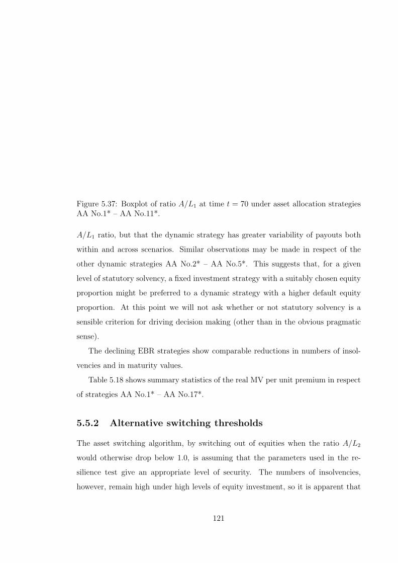
Figure 5.37: Boxplot of ratio A/L1 at time t = 70 under asset allocation strategiesAA No.1* – AA No.11*.
A/L1 ratio, but that the dynamic strategy has greater variability of payouts both
within and across scenarios. Similar observations may be made in respect of the
other dynamic strategies AA No.2* – AA No.5*. This suggests that, for a given
level of statutory solvency, a fixed investment strategy with a suitably chosen equity
proportion might be preferred to a dynamic strategy with a higher default equity
proportion. At this point we will not ask whether or not statutory solvency is a
sensible criterion for driving decision making (other than in the obvious pragmatic
sense).
The declining EBR strategies show comparable reductions in numbers of insol-
vencies and in maturity values.
Table 5.18 shows summary statistics of the real MV per unit premium in respect
of strategies AA No.1* – AA No.17*.
5.5.2 Alternative switching thresholds
The asset switching algorithm, by switching out of equities when the ratio A/L2
would otherwise drop below 1.0, is assuming that the parameters used in the re-
silience test give an appropriate level of security. The numbers of insolvencies,
however, remain high under high levels of equity investment, so it is apparent that
121

Ratio A/L1 Real MV per unit prem.
Strategy No. < 1 Ei(mint) Si(mint) Eit Si(Et) Ei(St) Corr
Fixed defaults
AA No.1* 276 1.040 0.095 10.264 1.716 3.071 0.143AA No.2* 216 1.059 0.091 10.294 1.660 2.965 0.152AA No.3* 143 1.084 0.088 10.289 1.583 2.837 0.175AA No.4* 81 1.114 0.089 10.258 1.511 2.702 0.153AA No.5* 35 1.152 0.092 10.171 1.453 2.556 0.133AA No.6* 12 1.204 0.089 10.036 1.421 2.417 0.113AA No.7* 2 1.266 0.074 9.873 1.397 2.297 0.140AA No.8* 0 1.328 0.055 9.703 1.391 2.209 0.207AA No.9* 0 1.387 0.040 9.540 1.402 2.165 0.297AA No.10* 0 1.442 0.031 9.379 1.430 2.171 0.417AA No.11* 0 1.478 0.029 9.214 1.468 2.220 0.503
Declining EBR defaults
AA No.12* 187 1.071 0.089 10.283 1.610 2.805 0.168AA No.13* 96 1.114 0.094 10.208 1.486 2.578 0.127AA No.14* 42 1.170 0.103 10.010 1.441 2.502 0.068AA No.15* 28 1.215 0.110 9.783 1.464 2.669 −0.014AA No.16* 176 1.080 0.091 10.204 1.531 2.657 0.088AA No.17* 6 1.219 0.090 9.878 1.407 2.310 0.113
Table 5.18: Comparison of ratio A/L1 with real Maturity Values, strategies AANo.1* – AA No.17* (solvency-driven investment strategies).
122

Strategy Ratio Switching threshold
AA No.18 A/L2 1.05AA No.19 A/L2 1.10AA No.20 A/L1 1.10AA No.21 A/L1 1.20
Table 5.19: Definition of Asset Allocation Strategies AA No.18 – AA No.21 (alter-native switching criteria.
Ratio A/L1 MV per unit prem.
Strategy No. < 1 Ei(mint) Si(mint) Eit Si(Et) Ei(St) Corr
100% in equities by default
AA No.18 162 1.079 0.089 16.679 2.743 4.647 0.329AA No.19 89 1.120 0.086 16.471 2.655 4.488 0.297AA No.20 513 0.986 0.128 17.022 2.924 4.884 0.418AA No.21 293 1.048 0.128 16.601 2.866 4.668 0.368
80% in equities by default
AA No.18 64 1.115 0.077 16.704 2.326 4.055 0.359AA No.19 33 1.151 0.070 16.509 2.261 3.962 0.329AA No.20 260 1.058 0.113 16.913 2.405 4.151 0.416AA No.21 132 1.110 0.098 16.575 2.394 4.029 0.456
Table 5.20: Comparison of ratio A/L1 with Maturity Values, strategies AA No.18 –AA No.21 (alternative solvency-driven investment strategies).
the switching criterion is not as successful as it might be.
Table 5.19 defines alternative switching strategies, based on different switching
thresholds and/or different financial ratios.
Strategies AA No.18 and AA No.19 both use the same ratio, A/L2, as the pre-
vious strategy, but begin to switch into gilts at a higher level, thus being more
conservative. We will call the level at which switching takes place the “switching
threshold”.
Strategies AA No.20 and AA No.21 use the ratio A/L1 (based on the statutory
minimum reserve ignoring the resilience reserve). Since this is a weaker test than
one using the ratio A/L2, higher switching thresholds are used.
Table 5.20 shows summary statistics of the nominal maturity values under these
switching strategies, with default investment strategies of 100% and 80% in equities.
The table shows that if the ratio A/L1 is used as a guide to asset switching it
is necessary to set a very high switching threshold; a threshold of 1.20 gives results
123

Ratio A/L1 Real MV per unit prem.
Strategy No. < 1 Ei(mint) Si(mint) Eit Si(Et) Ei(St) Corr
100% in equities by default
AA No.18 162 1.079 0.089 10.139 1.697 3.007 0.111AA No.19 89 1.120 0.086 10.020 1.667 2.929 0.073AA No.20 513 0.986 0.128 10.365 1.859 3.176 0.115AA No.21 293 1.048 0.128 10.118 1.832 3.076 0.048
80% in equities by default
AA No.18 64 1.115 0.077 10.189 1.586 2.796 0.162AA No.19 33 1.151 0.070 10.074 1.569 2.743 0.141AA No.20 260 1.058 0.113 10.324 1.647 2.880 0.106AA No.21 132 1.110 0.098 10.130 1.672 2.825 0.112
Table 5.21: Comparison of ratio A/L1 with real Maturity Values, strategies AANo.18 – AA No.21 (alternative solvency-driven investment strategies).
very similar to the use of the ratio A/L2 with a threshold of 1.00.
Comparing Tables 5.20 and 5.21 with Tables 5.10 and 5.11, it still appears that
the asset switching strategies have little advantage over a fixed strategy with a
suitably chosen level of equity investment. For example, compare strategy AA No.18
above (A/L2 = 1.05) with 100% in equities by default with strategy AA No.5, which
has a fixed 60% in equities. AA No.18 results in slightly more insolvencies (162) than
does AA No.5 (156), and the mean maturity values are similar, but the variability
of the maturity values (nominal or real) within and across scenarios is about the
same as that of strategy AA No.2, with a fixed 90% in equities. In other words,
for a given level of statutory insolvency the fixed investment strategies give similar
mean payouts with lower variability.
5.5.3 Limits on asset switching
The asset-switching algorithm permits switches of any size, so that the entire equity
holding may be liquidated in a single year. In practice this would be infeasible for a
large or medium sized life office. Even if its managers decided to run down its equity
holdings they would have to do so gradually; some equity-type assets are inherently
illiquid (such as properties) while disposal of large quantities of widely-traded stocks
would move the price adversely.
It follows that an asset-switching algorithm intended to ensure solvency might
124

Solvency-driven asset switching
Default rule None Unlimited 25% limit
100% equities 745 276 49780% equities 624 216 35570% equities 485 143 23660% equities 321 81 12150% equities 156 35 43
Table 5.22: Comparison of the numbers of statutory insolvencies with and withoutan asset switching limit of 25% of the fund per year.
be too optimistic if it allowed switches of arbitrary size to take place; the protection
of the solvency position might be a good deal less if there were more realistic limits
on asset switches.
To investigate this, strategies AA No.1* – AA No.5* have been modified so that
no more than 25% of the fund can be switched from equities to gilts or vice versa
in any one year. The limit is based on the value of the assets at the end of the year,
assuming that revenue cash-flows have been invested during the year in proportion
to the market value of the different asset types in the fund at market value. With
50% or less of the fund in equities to start with the extent of asset switching is much
reduced and we have omitted these.
Table 5.22 compares the number of statutory insolvencies with no switching
(from Table 5.10), with unrestricted switching (from Table 5.17) and with switching
restricted as above.
Comparing the second and third columns, the numbers of statutory insolvencies
are increased, by rather more when there is a high level of equity investment. Thus
much of the protection offered by the asset-switching is lost. This suggests that the
utility of solvency driven asset-switching might be considerably lower
than suggested by (for example) Ross or Ross & McWhirter. (In fairness
it should be noted that these authors were not advocates of solvency-driven asset
switching.)
125

5.6 Index-driven asset switching
Although the maintenance of solvency might occasionally impinge on asset alloca-
tion, investment policy is more usually driven by the managers’ views on likely stock
market behaviour. Markets are not static, and managers’ views will change in line
with experience, and asset allocations with them. Static strategies such as holding
fixed proportions of the fund in equities, or declining EBR strategies, represent ex-
tremely long-term views. Even managers who agreed with these views might depart
from the resulting allocations over short or medium terms as the market, or the
liabilities, dictated. Indeed, the declining EBR strategies will force switches out of
equities even when this would be far from sensible, for example when equity prices
are low and dividend yields high.
In this section we investigate the effect of some investment strategies which are
driven by the recent history of appropriate investment indices.
5.6.1 Cyclical and contracyclical strategies
In 1986 Waters [67] used the Wilkie asset model to explore the effect of different
investment strategies on the present value of the profit emerging under a single
cohort of non-profit endowment policies. Three of the strategies were:
Strategy EQ To invest each year’s cashflow entirely in equities.
Strategy FI To invest each year’s cashflow entirely in consols.
Strategy FE To invest each year’s cashflow in a mixture of equities and consols,
the proportion being weighted towards the better performing sector.
One of the interesting results was the effect of the mixed investment strategy.
Investment entirely in equities gave high mean profits with a high standard devia-
tion, and investment entirely in consols gave low mean profits with a low standard
deviation, but the mixed investment strategy FE achieved a combination of mean
profits only slightly lower than those uder Strategy EQ and a standard deviation
only a little higher than that under Strategy FI.
126

This mixed strategy FE might be termed “cyclical” because the direction of
investment moves in line with the market. Another set of strategies are termed
“contracyclical”. In these, the investor favours those sectors which have performed
relatively badly, on the grounds that this increases the chances of buying at the
bottom. Macdonald [42] found that contracyclical strategies outperformed cyclical
strategies, under the conditions of the Wilkie model.
Define the following indices in respect of equities and consols.
Let Pt be an index of equity prices, representing the value at time t of an invest-
ment of £1 at time 0, assuming that gross dividends are reinvested at the end of
every year. This is equivalent to
Pt =s=t∏s=1
(1 + es)
where es is the total gross rate of return on equities in year s, and we assume
that P0 = 1. Let Ct be an index representing the value at time t of an investment
of £1 in consols at time 0, assuming that gross interest payments are reinvested at
the end of every year. This is equivalent to
Ct =ct
c0
s=t∏s=1
(1 +i
cs
)
where i is the gross coupon rate and ct is the price of a single bond at time t.
This is because the initial investment buys 1c0
bonds. Each year the interest at rate
i on the current nominal holding is reinvested to increase the nominal holding by a
factor (1+ ics
), and at time t the value of the holding is ct times the nominal amount.
Then a simple cyclical strategy is to switch towards that sector which has seen
the greater increase in its index over the most recent period. We will look at changes
in the indices over the last 1, 2 and 3 years; we will give this time period the name
“index period”. For example, with an index period of 2 years we would switch
towards equities at time t if
Pt
Pt−2
>Ct
Ct−2
and towards gilts otherwise. In other words, we would switch towards equities if
PtCt−2
CtPt−2
> 1
127
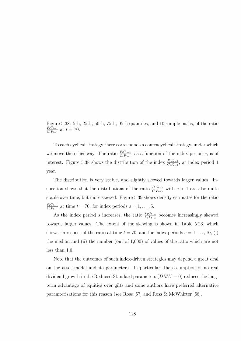
Figure 5.38: 5th, 25th, 50th, 75th, 95th quantiles, and 10 sample paths, of the ratioPtCt−1
CtPt−1at t = 70.
To each cyclical strategy there corresponds a contracyclical strategy, under which
we move the other way. The ratio PtCt−s
CtPt−s, as a function of the index period s, is of
interest. Figure 5.38 shows the distribution of the index PtCt−1
CtPt−1, at index period 1
year.
The distribution is very stable, and slightly skewed towards larger values. In-
spection shows that the distributions of the ratio PtCt−s
CtPt−swith s > 1 are also quite
stable over time, but more skewed. Figure 5.39 shows density estimates for the ratio
PtCt−1
CtPt−1at time t = 70, for index periods s = 1, . . . , 5.
As the index period s increases, the ratio PtCt−s
CtPt−sbecomes increasingly skewed
towards larger values. The extent of the skewing is shown in Table 5.23, which
shows, in respect of the ratio at time t = 70, and for index periods s = 1, . . . , 10, (i)
the median and (ii) the number (out of 1,000) of values of the ratio which are not
less than 1.0.
Note that the outcomes of such index-driven strategies may depend a great deal
on the asset model and its parameters. In particular, the assumption of no real
dividend growth in the Reduced Standard parameters (DMU = 0) reduces the long-
term advantage of equities over gilts and some authors have preferred alternative
paramterisations for this reason (see Ross [57] and Ross & McWhirter [58].
128

Figure 5.39: Estimates of the density of the ratio PtCt−s
CtPt−sfor s = 1, . . . , 5, at time
t = 70.
PtCt−s
CtPt−s
Index period s Median No. ≥ 1.0
1 1.014 5202 1.022 5233 1.036 5424 1.054 5365 1.081 5626 1.098 5637 1.093 5718 1.099 5609 1.120 57310 1.139 573
Table 5.23: Median and number (out of 1,000) of positive values of PtCt−s
CtPt−sat time
t = 70 for s = 1, . . . , 10.
129

Run length Pt CtPtCt−1
CtPt−1
Rises
1 2263 651 34782 1686 512 20813 1153 426 10714 807 372 5275 455 330 2536 297 247 1327 180 213 448 113 194 319 49 134 610 and over 98 921 6
Falls
1 4478 2658 38312 1633 466 20363 468 107 9564 145 20 4345 and over 37 8 317
Table 5.24: Numbers of runs of rising and falling index values in 1,000 simulationsover 30 years.
Cyclical strategies depend on the assumption that a rise in a given index is more
likely to be followed by another rise than by a fall. Contracyclical strategies assume
the opposite. It is therefore of interest to study the patterns of rises and falls of the
indices. Table 5.24 shows the numbers of uninterrupted runs of rises and falls in Pt,
Ct and PtCt−1
CtPt−1in the 1,000 scenarios used here.
Note that the data upon which these run lengths are based are censored since the
30,000 values of each index were based on 1,000 simulations each of length 30 years.
This should not affect the frequency with which runs of each length are observed.
Suppose that the ratio PtCt−1
CtPt−1, having risen for one or more years, then falls.
Then there are two possibilities; the fall is either a run of length 1 or the start of a
longer run of falls. From the table, the frequency of the first of these possibilities is
3831/7574 = 0.5058 ≈ 0.51. (The denominator is the total number of runs of falling
indices.) This offers practically no guidance. Given two successive falls, then the
frequency of a rise in the next year is 2036/3734 ≈ 0.54. Similarly, if we observe
one or two years of rising indices, the estimated probabilities of another rise in the
following year are 0.54 and 0.5 respectively. Table 5.25 shows the frequencies with
130
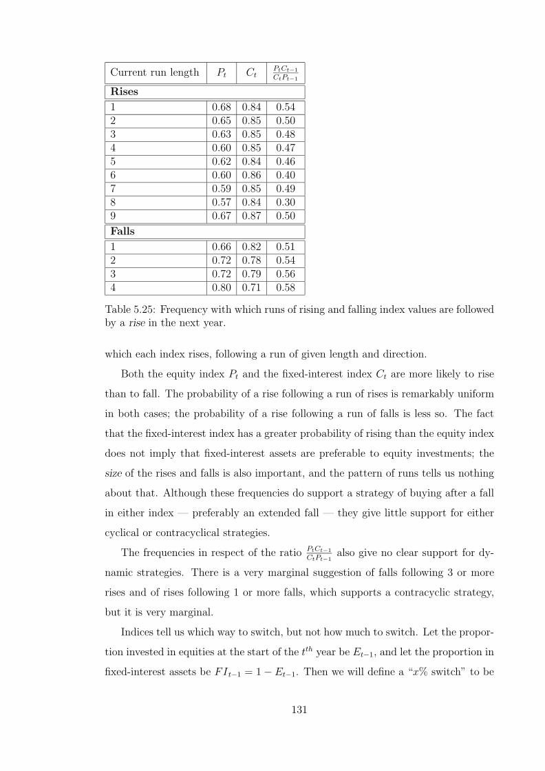
Current run length Pt CtPtCt−1
CtPt−1
Rises
1 0.68 0.84 0.542 0.65 0.85 0.503 0.63 0.85 0.484 0.60 0.85 0.475 0.62 0.84 0.466 0.60 0.86 0.407 0.59 0.85 0.498 0.57 0.84 0.309 0.67 0.87 0.50
Falls
1 0.66 0.82 0.512 0.72 0.78 0.543 0.72 0.79 0.564 0.80 0.71 0.58
Table 5.25: Frequency with which runs of rising and falling index values are followedby a rise in the next year.
which each index rises, following a run of given length and direction.
Both the equity index Pt and the fixed-interest index Ct are more likely to rise
than to fall. The probability of a rise following a run of rises is remarkably uniform
in both cases; the probability of a rise following a run of falls is less so. The fact
that the fixed-interest index has a greater probability of rising than the equity index
does not imply that fixed-interest assets are preferable to equity investments; the
size of the rises and falls is also important, and the pattern of runs tells us nothing
about that. Although these frequencies do support a strategy of buying after a fall
in either index — preferably an extended fall — they give little support for either
cyclical or contracyclical strategies.
The frequencies in respect of the ratio PtCt−1
CtPt−1also give no clear support for dy-
namic strategies. There is a very marginal suggestion of falls following 3 or more
rises and of rises following 1 or more falls, which supports a contracyclic strategy,
but it is very marginal.
Indices tell us which way to switch, but not how much to switch. Let the propor-
tion invested in equities at the start of the tth year be Et−1, and let the proportion in
fixed-interest assets be FI t−1 = 1− Et−1. Then we will define a “x% switch” to be
131
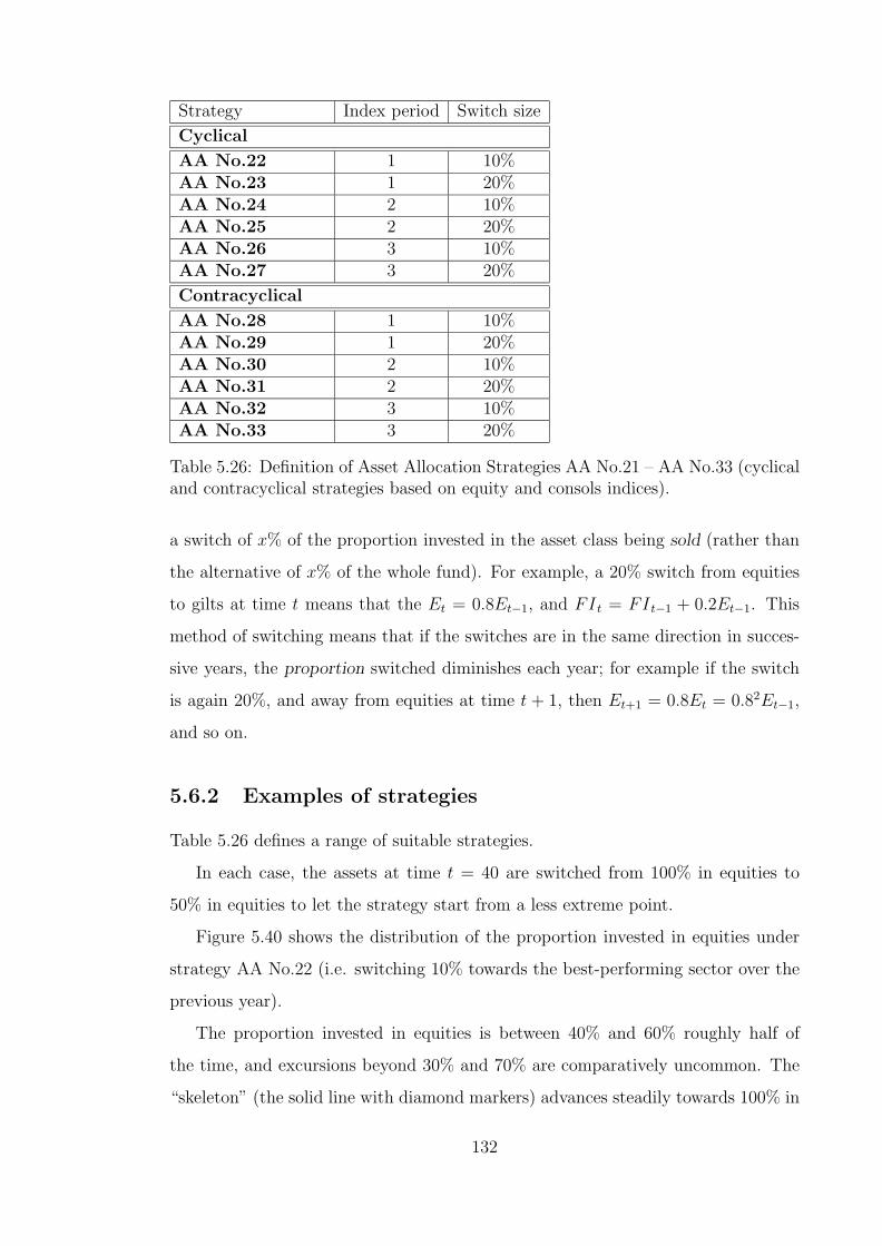
Strategy Index period Switch size
Cyclical
AA No.22 1 10%AA No.23 1 20%AA No.24 2 10%AA No.25 2 20%AA No.26 3 10%AA No.27 3 20%
Contracyclical
AA No.28 1 10%AA No.29 1 20%AA No.30 2 10%AA No.31 2 20%AA No.32 3 10%AA No.33 3 20%
Table 5.26: Definition of Asset Allocation Strategies AA No.21 – AA No.33 (cyclicaland contracyclical strategies based on equity and consols indices).
a switch of x% of the proportion invested in the asset class being sold (rather than
the alternative of x% of the whole fund). For example, a 20% switch from equities
to gilts at time t means that the Et = 0.8Et−1, and FI t = FI t−1 + 0.2Et−1. This
method of switching means that if the switches are in the same direction in succes-
sive years, the proportion switched diminishes each year; for example if the switch
is again 20%, and away from equities at time t + 1, then Et+1 = 0.8Et = 0.82Et−1,
and so on.
5.6.2 Examples of strategies
Table 5.26 defines a range of suitable strategies.
In each case, the assets at time t = 40 are switched from 100% in equities to
50% in equities to let the strategy start from a less extreme point.
Figure 5.40 shows the distribution of the proportion invested in equities under
strategy AA No.22 (i.e. switching 10% towards the best-performing sector over the
previous year).
The proportion invested in equities is between 40% and 60% roughly half of
the time, and excursions beyond 30% and 70% are comparatively uncommon. The
“skeleton” (the solid line with diamond markers) advances steadily towards 100% in
132
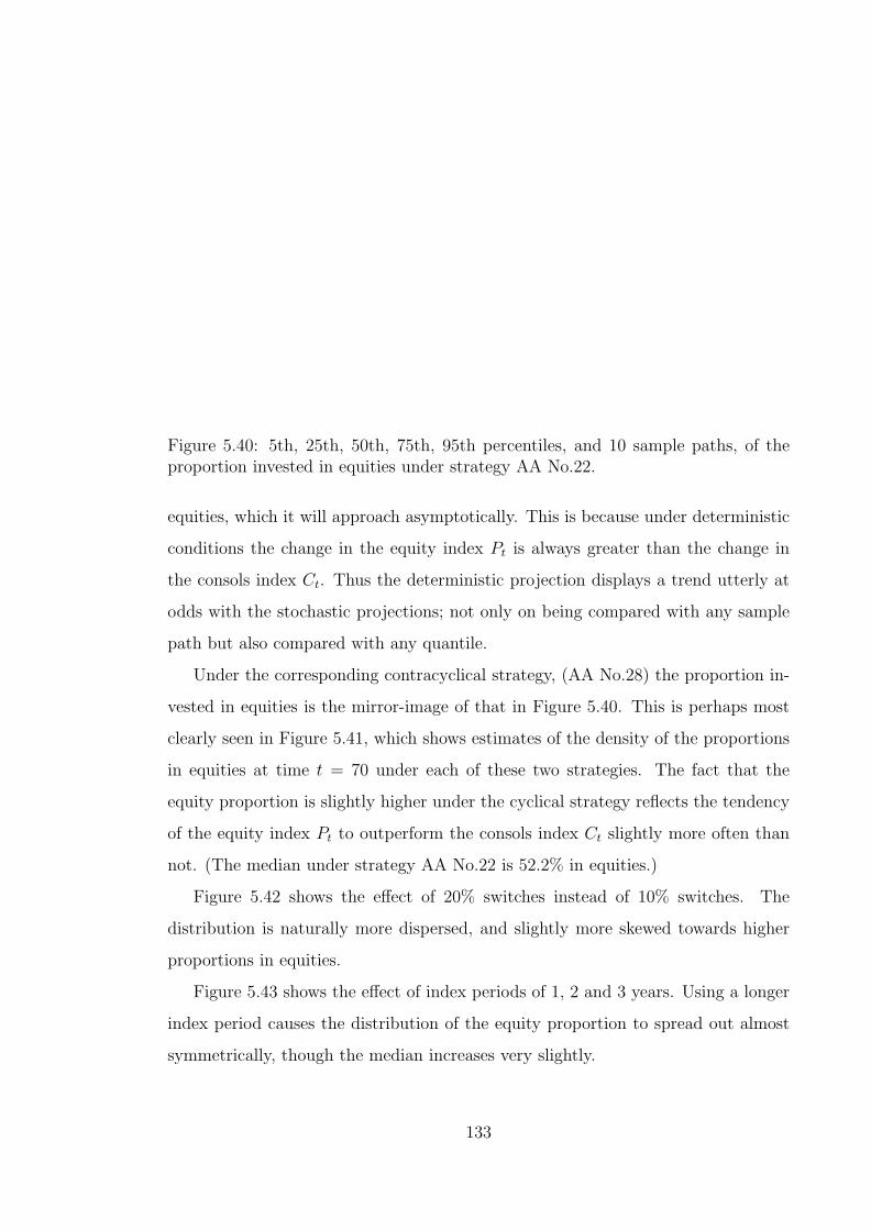
Figure 5.40: 5th, 25th, 50th, 75th, 95th percentiles, and 10 sample paths, of theproportion invested in equities under strategy AA No.22.
equities, which it will approach asymptotically. This is because under deterministic
conditions the change in the equity index Pt is always greater than the change in
the consols index Ct. Thus the deterministic projection displays a trend utterly at
odds with the stochastic projections; not only on being compared with any sample
path but also compared with any quantile.
Under the corresponding contracyclical strategy, (AA No.28) the proportion in-
vested in equities is the mirror-image of that in Figure 5.40. This is perhaps most
clearly seen in Figure 5.41, which shows estimates of the density of the proportions
in equities at time t = 70 under each of these two strategies. The fact that the
equity proportion is slightly higher under the cyclical strategy reflects the tendency
of the equity index Pt to outperform the consols index Ct slightly more often than
not. (The median under strategy AA No.22 is 52.2% in equities.)
Figure 5.42 shows the effect of 20% switches instead of 10% switches. The
distribution is naturally more dispersed, and slightly more skewed towards higher
proportions in equities.
Figure 5.43 shows the effect of index periods of 1, 2 and 3 years. Using a longer
index period causes the distribution of the equity proportion to spread out almost
symmetrically, though the median increases very slightly.
133

Figure 5.41: Density estimates of the proportion invested in equities at time t = 70under the cyclical strategy AA No.22 and the contracyclical strategy AA No.28.
0 20 40 60 80 100
0.0
0.01
0.02
0.03
Figure 5.42: Density estimates of the proportion invested in equities at time t = 70under the cyclical strategies AA No.22 (10% switches) and AA No.23 (20% switches).
134
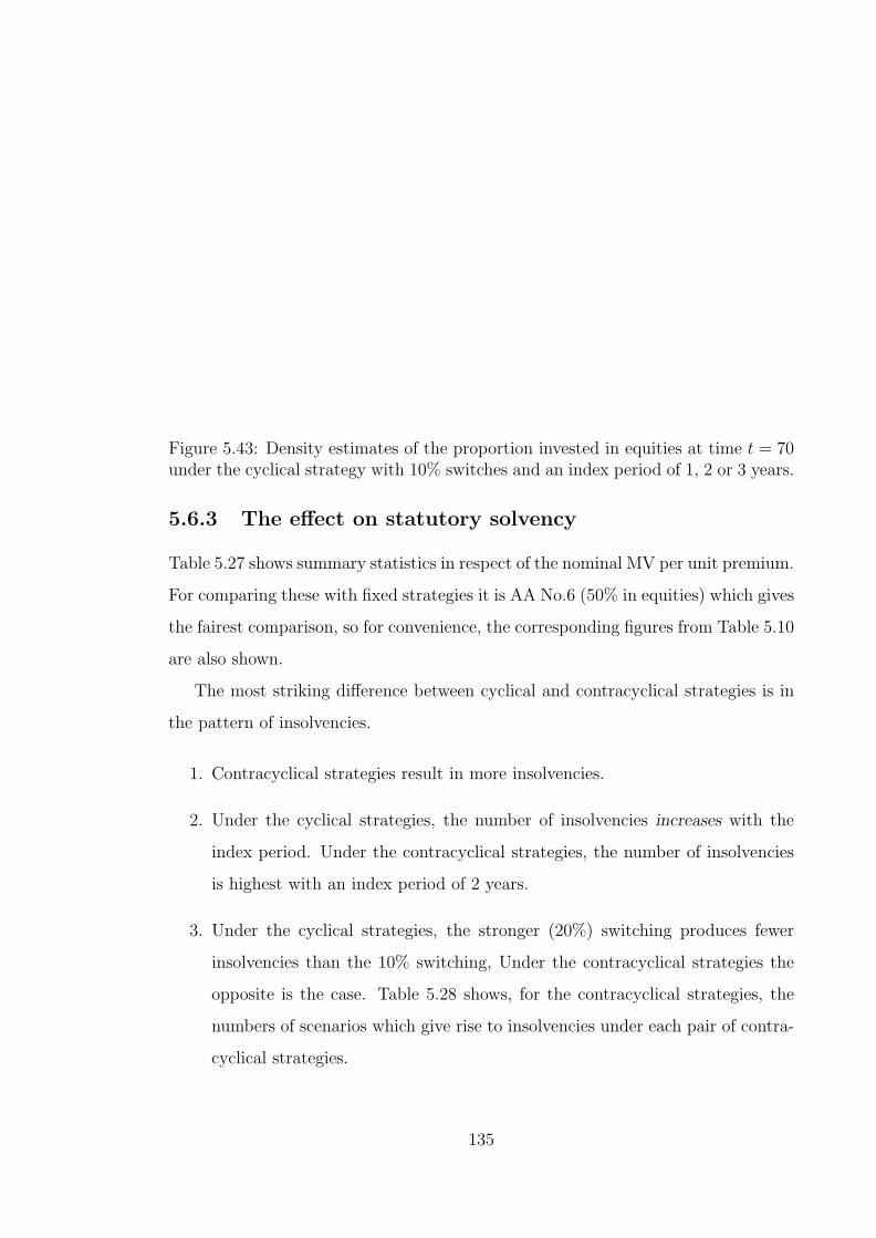
Figure 5.43: Density estimates of the proportion invested in equities at time t = 70under the cyclical strategy with 10% switches and an index period of 1, 2 or 3 years.
5.6.3 The effect on statutory solvency
Table 5.27 shows summary statistics in respect of the nominal MV per unit premium.
For comparing these with fixed strategies it is AA No.6 (50% in equities) which gives
the fairest comparison, so for convenience, the corresponding figures from Table 5.10
are also shown.
The most striking difference between cyclical and contracyclical strategies is in
the pattern of insolvencies.
1. Contracyclical strategies result in more insolvencies.
2. Under the cyclical strategies, the number of insolvencies increases with the
index period. Under the contracyclical strategies, the number of insolvencies
is highest with an index period of 2 years.
3. Under the cyclical strategies, the stronger (20%) switching produces fewer
insolvencies than the 10% switching, Under the contracyclical strategies the
opposite is the case. Table 5.28 shows, for the contracyclical strategies, the
numbers of scenarios which give rise to insolvencies under each pair of contra-
cyclical strategies.
135

Ratio A/L1 MV per unit prem.
Strategy No. < 1 Ei(mint) Si(mint) Eit Si(Et) Ei(St) Corr
Fixed 50% in equities
AA No.6 42 1.198 0.1 16.356 1.571 2.761 0.142Cyclical
AA No.22 29 1.207 0.092 16.315 1.771 2.958 −0.113AA No.23 20 1.224 0.089 16.283 1.873 3.107 −0.122AA No.24 47 1.195 0.101 16.252 1.814 2.988 −0.168AA No.25 40 1.206 0.100 16.158 1.934 3.170 −0.180AA No.26 63 1.179 0.109 16.249 1.895 3.039 −0.213AA No.27 58 1.183 0.110 16.140 2.053 3.251 −0.216
Contracyclical
AA No.28 102 1.177 0.132 16.404 1.436 2.617 0.252AA No.29 165 1.142 0.157 16.444 1.422 2.569 0.251AA No.30 102 1.183 0.134 16.472 1.427 2.613 0.276AA No.31 176 1.145 0.161 16.578 1.438 2.580 0.282AA No.32 94 1.191 0.136 16.483 1.383 2.597 0.290AA No.33 157 1.151 0.167 16.615 1.399 2.585 0.300
Table 5.27: Comparison of ratio A/L1 with Maturity Values, strategies AA No.22 –AA No.33 (cyclical and contracyclical strategies based on equity and consols indices)
StrategyStrategy AA 28 AA 29 AA 30 AA 31 AA 32 AA 33
AA No.28 102 102 79 95 72 87AA No.29 102 165 92 136 82 117
AA No.30 79 92 102 101 80 90AA No.31 95 136 101 176 89 129
AA No.32 72 82 80 89 94 94AA No.33 87 117 90 129 94 157
Table 5.28: Numbers of scenarios (out of 1,000) giving rise to statutory insolvencyunder each pair of contracyclical strategies AA No.28 – AA No.33.
136

MV cit
MV ccit
Strategies Index period Switch size Eit Si(Et) Ei(St)
AA No.22/28 1 10% 0.992 0.035 0.053AA No.23/29 1 20% 0.989 0.057 0.089AA No.24/30 2 10% 0.984 0.043 0.064AA No.25/31 2 20% 0.975 0.069 0.106AA No.26/32 3 10% 0.984 0.053 0.076AA No.27/33 3 20% 0.973 0.084 0.124
Table 5.29: Comparison of ratio MV cit
MV ccit
of Maturity Values under cyclic strategies
(MV cit ) to Maturity Values under contracyclic strategies (MV cci
t ).
Therefore the effect of increasing the switch size is largely to make more of-
fices insolvent, in addition to those already insolvent. This is not always (or
even usually) the case following a change in strategy; often the sets of scenar-
ios resulting in insolvency under two different strategies have a more modest
intersection.
5.6.4 The effect on maturity values
There is also a striking difference between the maturity values under the cyclical
and contracyclical strategies. Each contracyclical strategy results in a higher mean
MV per unit premium (Eit(MV i
t)) than its cyclical counterpart. This makes some
intuitive sense, since a contracyclical strategy aims to buy low and sell high. How-
ever, each contracyclical strategy also results in lower variability than its cyclical
counterpart, both between scenarios and within scenarios. The difference appears
to increase with the index period.
Table 5.29 shows the summary statistics of the ratio of maturity values under
each cyclical strategy to those under its corresponding contracyclical strategy, calcu-
lated path-by-path. That is, let MV cit be the MV per unit premium at time t in the
ith scenario under a cyclical strategy, and let MV ccit be the MV per unit premium
at time t in the ith scenario under the corresponding contracyclical strategy. Then
form the ratio MV cit
MV ccit
, and compute summary statistics Eit(
MV cit
MV ccit
) etc. as before.
This confirms that the cyclical strategies give lower maturity benefits
on average, although the variability, especially within scenarios, suggests that this
137

Figure 5.44: 5th, 25th, 50th, 75th, 95th percentiles, and 10 sample paths, of the
ratio MV cit
MV ccit
under strategies AA No.27 (cyclical) and AA No.33 (contracyclical).
might be far from uniformly true within each scenario. However, the distribution of
the ratio MV cit
MV ccit
is skewed: Figure 5.44 shows the distribution in the case of strategies
AA No.27 (cyclical) and AA No.33 (contracyclical).
In about 75% of cases, the ratio is below 1.0, indicating that the cyclical strategy
is poorer than the contracyclical strategy. The 95th quantile is very high, which
means that the mean ratio Eit(
MV cit
MV ccit
) shown in Table 5.29 understates the advantage
possessed by the contracyclical strategy. Inspection shows similar skewness in the
distribution of the ratio MV cit
MV ccit
under the other strategies.
Another interesting feature of Figure 5.44 is the anomalous behaviour of the
deterministic projection (the solid line with diamond markers). It shows again how
deterministic projections might lead to misleading results. In this case, the question
at issue is the relative effect of a pair of alternative asset allocation strategies,
given two asset classes, one of which yields higher returns in the long-run average.
Deterministic projections would lead us to prefer the wrong strategy.
Figure 5.45 shows a box plot of the MV per unit premium under the fixed
(50%) strategy, and the cyclical and contracyclical strategies. It is apparent that
the differences between the latter two lie mainly in the maturity values under the
cyclical strategies having a much longer tail towards higher values; nevertheless each
138

Figure 5.45: Boxplot of the MV per unit premium at time t = 70 under assetallocation strategies AA No.6 and AA No.22 – AA No.33.
contracyclical strategy has a higher median than its cyclical couterpart.
Moreover, comparing these dynamic strategies with fixed 50% in eq-
uities, the cyclical strategies all result in lower mean benefits with higher
variability, while the contracyclical strategies all result in higher mean
benefits with lower variability. Figure 5.46 shows the distribution of the ratio
MV cit
MV ccit
in the case of strategies AA No.33 (contracyclical) and AA No.6 (fixed 50%
equities).
Note that this figure is “upside-down” compared with Figure 5.44, in that the
contracyclical strategy provides the numerator of the ratio. It shows that there is
a similar skewness to the distribution of the ratio, so that the relative advantage of
the contracyclical strategy is understated by the comparison of the means in Table
5.27.
Contracyclical strategies appear to offer the best of both worlds; higher mean
benefits with lower variability. Cyclical strategies appear to be outperformed in
this regard even by the fixed asset allocation strategy. However, the success of the
contracyclical strategies is purchased at the price of considerably more statutory
insolvencies. This leads again to the question of whether or not the statutory min-
imum valuation, insofar as it might drive the asset allocation strategy, is acting
appropriately, to which we return in Chapter 7.
139
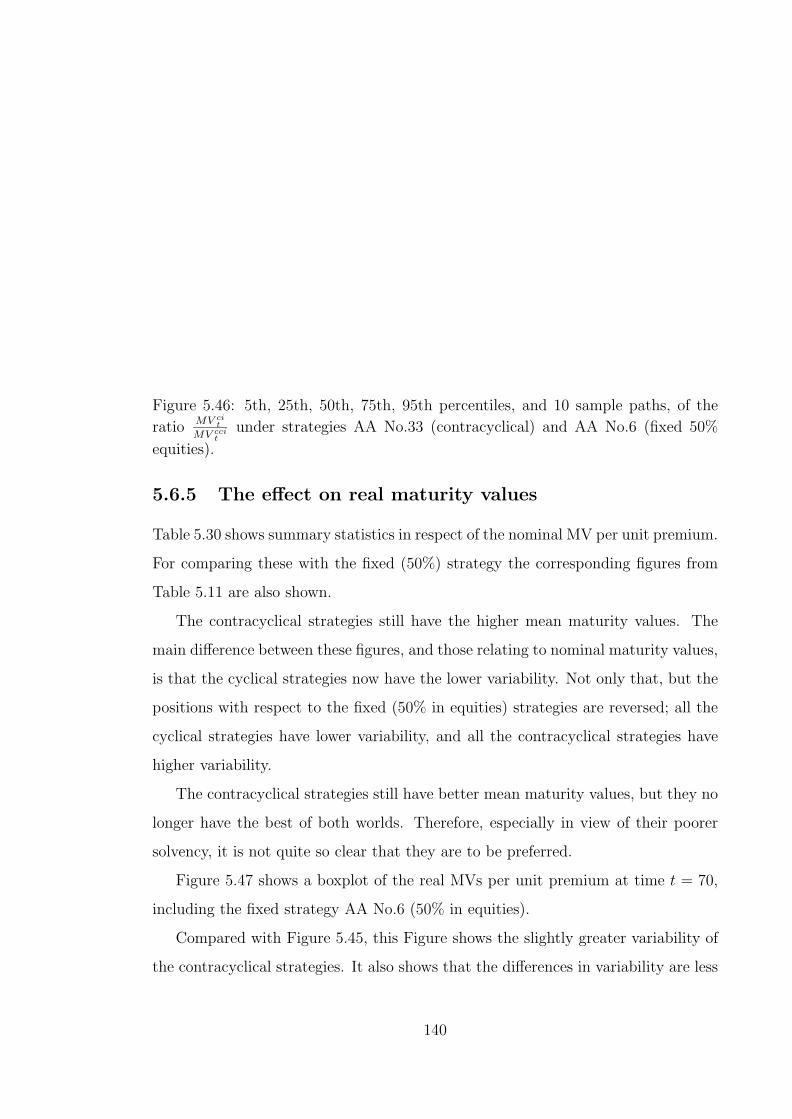
Figure 5.46: 5th, 25th, 50th, 75th, 95th percentiles, and 10 sample paths, of the
ratio MV cit
MV ccit
under strategies AA No.33 (contracyclical) and AA No.6 (fixed 50%
equities).
5.6.5 The effect on real maturity values
Table 5.30 shows summary statistics in respect of the nominal MV per unit premium.
For comparing these with the fixed (50%) strategy the corresponding figures from
Table 5.11 are also shown.
The contracyclical strategies still have the higher mean maturity values. The
main difference between these figures, and those relating to nominal maturity values,
is that the cyclical strategies now have the lower variability. Not only that, but the
positions with respect to the fixed (50% in equities) strategies are reversed; all the
cyclical strategies have lower variability, and all the contracyclical strategies have
higher variability.
The contracyclical strategies still have better mean maturity values, but they no
longer have the best of both worlds. Therefore, especially in view of their poorer
solvency, it is not quite so clear that they are to be preferred.
Figure 5.47 shows a boxplot of the real MVs per unit premium at time t = 70,
including the fixed strategy AA No.6 (50% in equities).
Compared with Figure 5.45, this Figure shows the slightly greater variability of
the contracyclical strategies. It also shows that the differences in variability are less
140

Ratio A/L1 Real MV per unit prem.
Strategy No. < 1 Ei(mint) Si(mint) Eit Si(Et) Ei(St) Corr
Fixed 50% in equities
AA No.6 42 1.198 0.1 10.057 1.42 2.423 0.077Cyclical
AA No.22 29 1.207 0.092 10.007 1.403 2.438 0.150AA No.23 20 1.224 0.089 9.974 1.407 2.461 0.142AA No.24 47 1.195 0.101 9.963 1.396 2.427 0.151AA No.25 40 1.206 0.100 9.888 1.401 2.443 0.167AA No.26 63 1.179 0.109 9.952 1.387 2.429 0.168AA No.27 58 1.183 0.110 9.863 1.392 2.446 0.183
Contracyclical
AA No.28 102 1.177 0.132 10.113 1.462 2.442 −0.019AA No.29 165 1.142 0.157 10.153 1.493 2.475 −0.012AA No.30 102 1.183 0.134 10.160 1.478 2.470 −0.030AA No.31 176 1.145 0.161 10.245 1.523 2.533 −0.015AA No.32 94 1.191 0.136 10.176 1.503 2.487 −0.069AA No.33 157 1.151 0.167 10.282 1.564 2.572 −0.058
Table 5.30: Comparison of ratio A/L1 with real Maturity Values, strategies AANo.22 – AA No.33 (cyclical and contracyclical strategies based on equity and consolsindices)
010
2030
4
AA6 AA22AA23AA24AA25AA26AA27AA28AA29AA30AA31AA32AA33
Figure 5.47: Boxplot of the real MV per unit premium at time t = 70 under assetallocation strategies AA No.6 and AA No.22 – AA No.33.
141
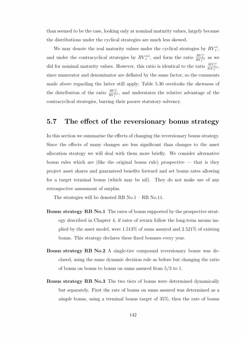
than seemed to be the case, looking only at nominal maturity values, largely because
the distributions under the cyclical strategies are much less skewed.
We may denote the real maturity values under the cyclical strategies by RV cit ,
and under the contracyclical strategies by RV ccit , and form the ratio RV ci
t
RV ccit
as we
did for nominal maturity values. However, this ratio is identical to the ratio MV cit
MV ccit
,
since numerator and denominator are deflated by the same factor, so the comments
made above regarding the latter still apply; Table 5.30 overlooks the skewness of
the distribution of the ratio RV cit
RV ccit
, and understates the relative advantage of the
contracyclical strategies, barring their poorer statutory solvency.
5.7 The effect of the reversionary bonus strategy
In this section we summarise the effects of changing the reversionary bonus strategy.
Since the effects of many changes are less significant than changes to the asset
allocation strategy we will deal with them more briefly. We consider alternative
bonus rules which are (like the original bonus rule) prospective — that is they
project asset shares and guaranteed benefits forward and set bonus rates allowing
for a target terminal bonus (which may be nil). They do not make use of any
retrospective assessment of surplus.
The strategies will be denoted RB No.1 – RB No.11.
Bonus strategy RB No.1 The rates of bonus supported by the prospective strat-
egy described in Chapter 4, if rates of return follow the long-term means im-
plied by the asset model, were 1.513% of sums assured and 2.521% of existing
bonus. This strategy declares these fixed bonuses every year.
Bonus strategy RB No.2 A single-tier compound reversionary bonus was de-
clared, using the same dynamic decision rule as before but changing the ratio
of bonus on bonus to bonus on sums assured from 5/3 to 1.
Bonus strategy RB No.3 The two tiers of bonus were determined dynamically
but separately. First the rate of bonus on sums assured was determined as a
simple bonus, using a terminal bonus target of 35%; then the rate of bonus
142
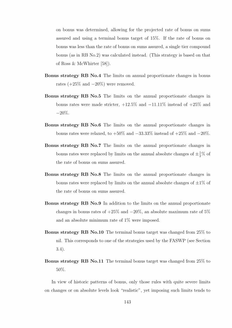
on bonus was determined, allowing for the projected rate of bonus on sums
assured and using a terminal bonus target of 15%. If the rate of bonus on
bonus was less than the rate of bonus on sums assured, a single tier compound
bonus (as in RB No.2) was calculated instead. (This strategy is based on that
of Ross & McWhirter [58]).
Bonus strategy RB No.4 The limits on annual proportionate changes in bonus
rates (+25% and −20%) were removed.
Bonus strategy RB No.5 The limits on the annual proportionate changes in
bonus rates were made stricter, +12.5% and −11.11% instead of +25% and
−20%.
Bonus strategy RB No.6 The limits on the annual proportionate changes in
bonus rates were relaxed, to +50% and −33.33% instead of +25% and −20%.
Bonus strategy RB No.7 The limits on the annual proportionate changes in
bonus rates were replaced by limits on the annual absolute changes of ±12% of
the rate of bonus on sums assured.
Bonus strategy RB No.8 The limits on the annual proportionate changes in
bonus rates were replaced by limits on the annual absolute changes of ±1% of
the rate of bonus on sums assured.
Bonus strategy RB No.9 In addition to the limits on the annual proportionate
changes in bonus rates of +25% and −20%, an absolute maximum rate of 5%
and an absolute minimum rate of 1% were imposed.
Bonus strategy RB No.10 The terminal bonus target was changed from 25% to
nil. This corresponds to one of the strategies used by the FASWP (see Section
3.4).
Bonus strategy RB No.11 The terminal bonus target was changed from 25% to
50%.
In view of historic patterns of bonus, only those rules with quite severe limits
on changes or on absolute levels look “realistic”, yet imposing such limits tends to
143

Figure 5.48: Boxplot of the rate of bonus on sums assured at time t = 70 under theoriginal bonus strategy and strategies RB No.1 – RB No.11.
push up the terminal bonus rates which are already high in Figure 4.7. However,
terminal bonus rates might be most naturally controlled by smoothing of maturity
values, which is discussed in Chapter 6.
Figure 5.48 shows a boxplot of the rates of bonus on sums assured at time t = 70
under these strategies; note that the plot labelled “Base” at the left-hand end is the
baseline office of Chapter 4 with the original strategy.
Table 5.31 shows the cumulative numbers of the 1,000 simulations under which
the ratio A/L1 ever fell below 1.0, by t = 50, t = 60 and t = 70. For convenience the
figures in respect of the “baseline” strategy described in Chapter 4 are also shown.
The details of the bonus rule have comparatively little impact on statutory insol-
vency, except in two cases. The exceptions are RB No.10 and RB No.11. Increasing
the terminal bonus target to 50% significantly reduces the incidence of statutory
insolvency, while decreasing it to nil significantly worsens statutory insolvency.
It is interesting that the number of insolvencies is lower if limits on changes in
bonus rates from year to year are removed completely (RB No.4) but higher if the
limits are merely relaxed (RB No.6). In addition, the imposition of absolute limits
of 1% and 5% (RB No.9) increases the number of insolvencies. This suggests that
the ability to reduce bonus rates quickly is a key factor in the influence of bonus
policy on solvency. Overall, though, the precise form of the limits on bonus changes
144

Cumulative No. of statutory insolvenciesBonus rule t = 50 t = 60 t = 70
Baseline 104 195 276RB No.1 108 207 290RB No.2 102 188 285RB No.3 109 226 333RB No.4 92 169 240RB No.5 106 192 278RB No.6 104 199 295RB No.7 96 185 289RB No.8 108 212 317RB No.9 105 201 293RB No.10 169 345 438RB No.11 82 139 196
Table 5.31: Cumulative number out of 1,000 simulations ever statutorily insolvent(A/L1 < 1) after 10, 20 and 30 years under prospective bonus strategies.
has a relatively small effect.
Figure 5.49 shows a boxplot of the ratio A/L1 at time t = 70.
The most striking change is that of strategy RB No.10, with a terminal bonus
target of nil. In this case the distribution is closely concentrated around A/L1 = 1.0,
with little skewness. A nil terminal bonus target is of course not sensible given high
equity investment; the interesting point is that the conclusions of the FASWP (see
Section 3.4) were based upon a similar bonus strategy. This result suggests that the
FASWP’s conclusions should perhaps not be compared with later work such as that
of Ross [57] and Ross & McWhirter [58].
Apart from RB No.10, all the amended strategies show slight variations on the
same theme. Compared with, for example, Figure 5.37, there is less evidence of
qualitative differences arising from the different strategies.
Similarly, there is little difference in the distributions of maturity values, except
under strategy RB No.10 where maturity values are much lower. This is because, as
long as the policy asset share is higher than the guarantees at maturity, the benefit
will be the same except insofar as the different build-up of liabilities has led to a
different investment strategy. Details of the maturity values and terminal bonus
rates are omitted.
145
Figure 5.49: Boxplot of the ratio A/L1 at time t = 70 under the original bonusstrategy and strategies RB No.1 – RB No.11.
So far as these 10-year policies are concerned, reasonable changes to the prospec-
tive reversionary bonus strategy affect the outcome less than do changes to the asset
allocation strategy. It is possible that bonus strategy should have a more significant
effect on longer term policies, under which the bonus additions will usually form a
larger portion of the guaranteed benefits at maturity.
5.8 Conclusions
1. Equity investment results in considerably higher mean maturity values than
does gilt investment, but also much greater variance of maturity values.
2. Statutory solvency is much worse under equity investment.
3. Alternative asset allocation strategies (solvency-driven switching, declining
EBR) appear to offer little advantage over fixed investment strategies, for
a given level of statutory insolvency.
4. Solvency-driven asset switching as used by Ross [57] and others is much less
effective if limits exist on the speed with which assets can be switched.
5. On the basis of nominal maturity values, the contracyclical strategies used
146

here perform better than their cyclical counterparts; they result in higher
mean maturity values with less variability. They are also slightly better than
the corresponding fixed investment strategy.
6. Consideration of real instead of nominal maturity values leads to
different conclusions.
• Comparing different levels of gilt and equity investment, the difference
in mean maturity values persists but the difference in volatility is much
reduced. Therefore investment in equities does not carry such a
significant penalty of relative volatility as is often supposed.
• Comparing cyclical and contracyclical investment strategies, the cyclical
strategies now have the less volatile (real) maturity values.
7. Changes to the reversionary bonus strategy make relatively little difference,
possibly due in part to the short term of the business. The change with the
greatest effect was to alter the terminal bonus target
147
Chapter 6
Smoothing with-profit maturity
values
In this chapter we consider the smoothing of with-profit maturity values. The effect
of smoothing is to pay out an amount other than the policy asset share at matu-
rity; sometimes more and sometimes less. These differences represent the cost of
smoothing. An important question is: does the cost of smoothing tend to stabilise
over time, or is the long term accumulated cost of smoothing unstable?
The existence of the guarantees provides another reason for sometimes paying
more than the asset share at maturity, and this too has a cost which ought to be
charged for. A further question is: if smoothing takes place anyway, is the cost
of meeting the guarantees absorbed into the cost of smoothing? If it is, does this
reduce the need to charge for the guarantees?
To consider these questions, we will introduce some possible smoothing meth-
ods based on practitioners’ responses to a survey, and then study the accumulated
costs of smoothing (the “Bonus Smoothing Account”) and of further meeting the
guarantees (the “Guarantee Cost Account”).
6.1 Introduction
Most U.K. with-profit offices claim to operate some form of smoothing of maturity
benefits. In part this is seen as an intrinsic feature of with-profit business, and one
148

which distinguishes it from unit-linked business, and as such it needs no explanation.
There are other reasons for smoothing based upon the operation of the guarantees,
particularly in an expanding office.
It is obvious that to pay 100% of asset shares as a minimum benefit when a claim
arises is a one-way process. An office which pursues such a policy is in the position of
providing subsidies out of its additional estate without the opportunity to replenish
that resource. It might not be so obvious that under some circumstances such a
policy need not prove ruinous.
It is well known that a life office whose rate of new business growth exceeds the
rate of return it can earn on its funds will eventually run out of capital. See, for
example, Smart [63]. The reason is that the requirement for capital grows along
with the new business, while unemployed capital grows at the rate of return on the
assets. However, in a with-profits office which pays a high proportion of the benefits
in the form of terminal bonus this restriction might be relaxed.
Consider a simplified life office, writing endowment business of term n years. It
is in a state of steady expansion, at rate e per annum, and it earns a rate of return
g on its assets. It has always paid 100% of asset shares to maturing policies, so its
total assets (ignoring any additional estate) are exactly equal to the total of its asset
shares at any time. In year t, the cash-flows are as follows:
Pt = Premiums received
Ct = Claims paid
Et = Expenses incurred
∆Vt = Change in reserve during the year
Then the total cashflow during year t is given by
CF t = gVt + Pt − Ct − Et −∆Vt
But because the office is expanding steadily at rate e per year,
Vt+1 = Vt(1 + e)
149

so
CF t = (g − e)Vt + Pt − Ct − Et
Consider now the office’s total asset shares at time t + 1, ASt+1.
ASt+1 = ASt(1 + g) + Pt − Ct − Et
but because of the uniform expansion
ASt+1 = ASt(1 + e)
so
ASt(e− g) = Pt − Ct − Et
and
CF t = (g − e)(Vt − ASt)
For the office to be able to finance expansion internally, the cash-flow CF t must
be non-negative. If the office made no use of terminal bonus, and attempted to
pay 100% of the asset share on claims by means of reversionary bonus, then almost
certainly Vt would exceed ASt (because there would be some conservatism in the
valuation basis) which tells us that (i) such a strategy would be infeasible without
additional capital, and (ii) such a strategy would only be sustainable if g > e. This
is the conventional result, that the rate of return on the assets limits the rate of new
business growth in the long run.
If, however, the office made use of terminal bonus, then for some values of e in
excess of g, it might be able to reduce its reserves to the point where, in aggregate,
Vt < ASt. Then the overall cash-flow would remain positive and expansion could
proceed at a higher rate.
If e > g, then the office must lose any additional estate which it possesses. If we
denote the total assets at time t by At, and the additional estate by AEt, then
At+1
ASt+1
=ASt+1 + AEt+1
ASt+1
= 1 +(1 + g)AEt
(1 + e)ASt
150

Therefore continued expansion at rate e > g will result in the ratio A/AS tending
to 1, i.e. in the loss of the additional estate, in relative terms. Note that this is true
if AEt < 0 as well as if AEt > 0, implying that rapid expansion financed by terminal
bonus is a way of escaping from a deficit in the assets — hardly to be recommended
in practice, though.
Passing on from this simple model, life offices in practice are not so stable,
and it is a matter of importance to maintain an adequate margin of assets over
liabilities, but new business expansion is usually also sought. As a minimum, some
expansion is needed to control cost inflation. Therefore offices will have regard to
the maintenance of any additional estate which they possess.
Smoothing of benefits therefore appears to be desirable. In bad times, the matu-
rity benefits will be subsidised, possibly at a level above that of the guarantees, and
this will be paid for by a charge on the asset shares of policies maturing in better
times. It is possible, therefore, that over the long term, smoothing will absorb the
cost of meeting the guarantees.
We will consider smoothing in a wider sense here, to include any form of ad-
justment to the asset shares of maturing policies, including “one-way” adjustments
such as the deduction of a uniform levy.
Our intuitive idea of smoothing is of a cost-neutral operation. We would like the
plusses and minuses to balance out, in the long run. It is not immediately obvious
that this will be the case, certainly not in all circumstances. For example, what
happens to the cost of smoothing if the office is expanding? Then each generation
of maturing policies will be bigger than its predecessors, and will either draw upon
or contribute to the office’s estate to a greater extent, depending on which way the
smoothing is then working.
In this chapter we examine the long-term cost of smoothing in a simple model
office.
151

6.2 Smoothing methods and the Bonus Smooth-
ing Account
A survey carried out by a firm of consultants [65] revealed that, of the 38 U.K.
with-profit offices which responded, 24 smoothed maturity values by limiting the
percentage change from year to year, 16 made projections of asset shares in an
attempt to smooth prospectively, and 11 calculated smoothed asset shares as a
basis for maturity values. 10 offices claimed to limit the cost of over- or under-
payment of maturity values. We will therefore use three smoothing approaches —
asset smoothing and maturity value smoothing, alone or in combination.
6.2.1 Asset smoothing
Section 4.1.3 described how the assets are valued actuarially using moving average
yields. This results in a smoother progression of asset values than does the market
valuation, so one simple approach to smoothing benefits is to pay the smoothed
value of the assets underlying the asset share of the maturing policy, instead of the
market value (subject to a minimum of the guaranteed benefits. We will call this
method “asset smoothing”.
The model office program uses a crude matching strategy to select dated gilts.
It first determines what proportion of the assets underlying the asset share of an
individual policy should be invested in gilts, and then allocates the appropriate
quantity of gilts of the same outstanding term as the policy. In other words, the
gilt component of the asset share of a policy with n years to run is always invested
in gilts with n years to redemption. This contrasts with the assumptions of (for
example) Ross & McWhirter, who used gilts of a fixed term to redemption.
This strategy means that only equities contribute to the smoothing of maturity
values — the actuarial value of a gilt on its redemption date is the same as its market
value, and the redemption date is also the maturity date of the corresponding policy.
Any smoothing which occurs when assets are entirely invested in gilts must therefore
be smoothing in a negative sense, due to the action of the guarantees.
Figure 6.50 shows how the ratio
152

Figure 6.50: 5th, 25th, 50th, 75th, 95th percentiles, and 10 sample paths, of theratio of the actuarial value and market value of the assets in the baseline office.
Actuarial Value of assets
Market Value of assets
(or the ratio AV /MV for short) progresses over time in the baseline office of
Chapter 4.
This ratio is slightly skewed towards values below 1.0. Inspection shows that this
is due to the pattern of asset switching. Times when the AV /MV ratio might be
high correspond to times of rising dividend yields and falling share prices, including
those circumstances in which the office is forced to switch into gilts. Investment in
gilts will cause the overall AV /MV ratio to be closer to 1.0 because the AV /MV
ratio for gilts is less volatile than for equities.
In fact, the distribution of the AV /MV ratio for equities alone is almost exactly
symmetrical.
6.2.2 Maturity value smoothing
An alternative, and more direct, smoothing method is to limit the change in maturity
values each year. However, maturity values increase naturally because the average
premium is assumed to increase with inflation, so to eliminate this effect we use the
153
maturity value per unit premium instead. We often abbreviate this to “MV per unit
premium” or just “MV per UP”.
Using this method, the calculated maturity value per unit premium is not allowed
to increase by more than 10% or to decrease by more than 9.09% in one year. These
figures were chosen so that the greatest increase followed by the greatest decrease
cancel out.
6.2.3 Combined smoothing
In some cases we use both smoothing methods together. The order in which the
calculations are then carried out is as follows:
1. The actuarial value of the assets underlying the asset share of the maturing
policy is calculated, and 100% of this is taken as the starting point.
2. The resulting maturity value per unit premium is not allowed to increase by
more than 10% or to decrease by more than 9.09% in one year.
3. If the guaranteed benefits exceed the maturity value limited as above the
former are paid.
6.2.4 The Bonus Smoothing Account
The Bonus Smoothing Account (BSA) was introduced by Lang & Scott [38]. It
is defined, for our purposes, as the accumulation of the differences between the
maturity values paid in the past, and the asset shares (at market valuation) of those
maturing policies. The accumulation is at the net rate of return on the fund.
Notice that no money changes hands, and the inflows to and outflows from
the BSA are notional and not physical cash-flows. The BSA is an internal book-
keeping item with no separate funds. Were it to be separately accounted for it would
correspond roughly to the equalisation reserve of a general insurance company.
In years when investment returns are particularly high, smoothing will tend to
keep maturity values below the underlying value of the assets, so there will then be a
contribution to the BSA from maturing policies. In years when investment returns
154

are particularly low, smoothing and perhaps also the guarantees will tend to keep
maturity values above the underlying value of the assets, so there will be a subsidy
from the BSA to maturing policies. Note that the BSA might increase even in the
latter circumstances, because of the assumed accumulation.
In this part of the work we focus on the ratio
Bonus Smoothing Account
Asset Shares
(or BSA/AS for short). The absolute value of the BSA tells us little. Dividing
by the total asset shares gives a relative measure of the impact of the BSA on the
finances of the office, from which any additional estate is removed. Changes in this
ratio might, of course, be due to changes in the asset shares rather than to changes
in the BSA.
6.2.5 The Guarantee Cost Account
If smoothing were so effective that the smoothed maturity values always exceeded
the guaranteed benefits, then the cost of meeting the guarantees would have been
absorbed completely into the cost of smoothing. If, however, the guarantees still
exceed the smoothed maturity values from time to time, then there will be an addi-
tional cost in meeting those guarantees, not absorbed into the cost of smoothing. If
we compare this with the cost of meeting the guarantees in the absence of smoothing,
we will be able to measure the extent to which the cost of smoothing has absorbed
the cost of meeting the guarantees.
Therefore define the Guarantee Cost Account (GCA) to be the accumulation
of the differences between the calculated maturity value, smoothed or unsmoothed
as the case may be, and the maturity benefit actually paid. Since the only time
this will be non-zero is when the guarantees are effective, the GCA measures the
cost of the guarantees, given the method used for calculating maturity values. Note
that the GCA as defined here is always zero or negative. We usually show the ratio
GCA/AS, for the same reasons as given above in respect of the BSA.
155

Asset share Cost of End-yearYear Unsmoothed Smoothed Guarantee Smoothing Guarantee BSA GCA
Without smoothing
1 100 n/a 90 n/a 0 n/a 02 95 n/a 92 n/a 0 n/a 03 104 n/a 94 n/a 0 n/a 04 92 n/a 95 n/a 3 n/a −35 90 n/a 96 n/a 6 n/a −9
With smoothing
1 100 97 90 −3 0 3 02 95 99 92 4 0 −1 03 104 101 94 −3 0 2 04 92 99 95 7 0 −5 05 90 92 96 2 4 −11 −4
Table 6.32: Example of the operation of the BSA and GCA, ignoring the effect ofinterest.
6.2.6 An example of the BSA and GCA
Table 6.32 sets out a simplified example of the operation of the BSA and the GCA.
In this example, the accumulation of both the BSA and the GCA at the fund rate
of return is ignored, and the table only shows the contributions each year to and
from the accounts.
First the operation of the GCA in the absence of smoothing is shown. In years
1, 2 and 3, the asset shares of maturing policies exceed the guaranteed benefits,
so there is no cost associated with the guarantees. In years 4 and 5, however, the
guarantees must be met, and the GCA is debited with the cost.
In the bottom half of the table, it is assumed that the asset shares of maturing
policies are smoothed as shown in the third column. In each of years 1, 2 and 3,
the difference between the smoothed and unsmoothed asset shares represents the
cost of smoothing, and this is debited from or credited to the BSA. In year 4, the
guaranteed benefits exceed the unsmoothed asset share but not the smoothed asset
share. Since the latter is paid, there is a cost associated with the smoothing but no
cost associated with the guarantees. In year 5 the guaranteed benefits exceed both
the smoothed and unsmoothed asset shares. The total cost of £6 is debited to the
BSA, but of this £4 represents the cost of meeting the guarantees after smoothing,
so is also debited to the GCA.
156
So with smoothing, the entire cost of meeting the guarantees is absorbed by the
normal operation of smoothing in Year 4, while only part of the cost is absorbed in
Year 5. It is seen that the GCA is part of the BSA — that part which represents
the “residual” cost of the guarantees after smoothing has absorbed what it can.
Alternative methods of meeting the cost of the guarantees have been explored,
for example by using options (see Wilkie [69]).
6.3 The effect of smoothing on benefits
6.3.1 Changes in maturity values
The effect of smoothing on maturity values can be studied by comparing the maturity
values paid with and without smoothing, within each simulation. We would expect
smoothing to reduce the differences between the maturity payouts in successive
years. Define
MV t = Unsmoothed MV per unit premium
MV at = MV per unit premium with asset smoothing
MV mt = MV per unit premium with maturity value smoothing
MV ct = MV per unit premium with combined smoothing
(See Figure 4.8 for the distribution of MV t.) Then let ∆MV t be the difference
MV t − MV t−1, and define ∆MV at , ∆MV m
t and ∆MV ct similarly. Figures 6.51 –
6.54 show the distributions of ∆MV t, ∆MV at , ∆MV m
t and ∆MV ct .
These figures show that asset smoothing on its own brings a significant reduction
in the changes of maturity values from year to year, but (comparing Figures 6.52 and
6.53) that changes in excess of 10% are still frequent. The maturity value smoothing
on its own or with asset smoothing has a much stronger effect than asset smoothing
alone on the more extreme quantiles, though the quartiles are very similar under
any of the smoothing methods.
157

Figure 6.51: 5th, 25th, 50th, 75th, 95th percentiles, and 10 sample paths, of thedifference ∆MV t with no smoothing.
40 45 50 55 60 65 70
-10
-50
Figure 6.52: 5th, 25th, 50th, 75th, 95th percentiles, and 10 sample paths, of thedifference ∆MV a
t with asset smoothing only.
158

Figure 6.53: 5th, 25th, 50th, 75th, 95th percentiles, and 10 sample paths, of thedifference ∆MV m
t with maturity value smoothing only.
40 45 50 55 60 65 70
-10
-50
Figure 6.54: 5th, 25th, 50th, 75th, 95th percentiles, and 10 sample paths, of thedifference ∆MV c
t with asset and maturity value smoothing.
159

Figure 6.55: 5th, 25th, 50th, 75th, 95th percentiles, and 10 sample paths, of theratio MV a
t
MV twith asset smoothing only.
6.3.2 The effect on individual policyholders
Figures 6.55 and 6.56 compare the smoothed with the unsmoothed maturity val-
ues. There, the ratio MV xt
MV t, where x = a or m within each simulation indicates the
difference which smoothing makes to the individual policyholder.
These Figures suggest that smoothing might have a very large effect on the
benefits of individual policyholders. Figure 6.55 naturally resembles Figure 6.50. It
might seem as if asset smoothing and maturity value smoothing had similar effects,
with the latter allowing slightly greater divergence from the unsmoothed values (as
befits the stronger smoother) but Figure 6.57 shows that this is not so. This shows
that the distribution of the ratio MV at
MV mt
is quite similar to those of the ratios MV at
MV tand
MV mt
MV t. The choice of smoothing method also makes a great difference to individual
payouts.
A feature of these figures is the small inter-quartile range. Although most sample
paths include some extreme values, the distribution is in fact quite tightly concen-
trated.
160

Figure 6.56: 5th, 25th, 50th, 75th, 95th percentiles, and 10 sample paths, of theratio MV m
t
MV twith maturity value smoothing only.
40 45 50 55 60 65 70
0.6
0.8
1.0
1
Figure 6.57: 5th, 25th, 50th, 75th, 95th percentiles, and 10 sample paths, of theratio MV a
t
MV mt
.
161

6.3.3 Summary measures of smoothness
In this section we consider summary measures of the effect of smoothing on maturity
benefits. As in Chapter 5, the differences caused by smoothing are observed within
each of the 1,000 scenarios, so we first summarise the differences within each scenario,
and then across all 1,000 scenarios.
Given a quantity X it defined at each time t = 1, . . . , n within each scenario
i = 1, . . . ,m, define Et(Xit), Ei(X i
t), Eit(X
it) etc. as in Section 5.2.
In this section let MV it denote the MV per unit premium at time t in the ith
scenario. Here we use the superscript i to denote the ith scenario and not, as before,
the smoothing method, since the latter will always be clear from the context. We
base our measures not on the MV per unit premium MV it but on a normalised MV
per unit premium NMV it. This makes comparison between different policies, and
between real and nominal maturity values, much easier. NMV it is defined as
NMV it =
MV it
Eit(MV i
t)
The measures which we show in Table 6.33 are the following:
Distribution of Et(|∆NMV it|). We have shown in Figures 6.51 – 6.54 the distri-
butions of the differences in the MV per unit premium from year to year.
It is more relevant to consider the absolute differences in a summary figure,
since the mean difference will clearly be close to 0. Within each scenario this
can be summarised by its (sample) mean and standard deviation. In respect
of the normalised MV per unit premium in the ith scenario denote these by
Et(|∆NMV it|) and St(|∆NMV i
t|) respectively, where the subscript t on SDt
indicates that the moments are calculated with respect to time. Then we sum-
marise the distribution of Et(|∆NMV it|) by its mean and standard deviation
over the 1,000 scenarios, denoted by Eit(|∆NMV i
t|) and Si(Et(|∆NMV it|))
respectively.
Mean of the s.d. of |∆NMV it|. The quantity Si(Et(|∆NMV i
t|)) sums up the range
of variation between different scenarios. If we reverse the order of the opera-
tions, and denote by Ei(St(|∆NMV it|)) the mean across all 1,000 scenarios of
St(|∆NMV it|), this will sum up the range of variation within scenarios.
162

Normalised MV per UP
Smoothing Eit(|∆NMV i
t|) Si(Et(|∆NMV it|)) Ei(St(|∆NMV i
t|))None (baseline) 0.136 0.049 0.145Asset smoothing only 0.087 0.032 0.087MV smoothing only 0.073 0.019 0.038Asset and MV smoothing 0.065 0.019 0.040
Non-normalised MV per UP
Smoothing Eit(|∆MV i
t|) Si(Et(|∆MV it|)) Ei(St(|∆MV i
t|))None (baseline) 2.306 0.826 2.445Asset smoothing only 1.427 0.517 1.425MV smoothing only 1.175 0.305 0.622Asset and MV smoothing 1.044 0.298 0.633
Table 6.33: Summary of distributions of |∆NMV it| and |∆MV i
t| with and withoutsmoothing.
In addition to the summary statistics based upon the normalised MV per unit
premium, Table 6.33 also shows the corresponding statistics based upon the
non-normalised MV per unit premium. These will be shown in this and the
following table only, for comparison with the normalised figures.
The features of Figures 6.51 – 6.54 are clearly shown in these summary figures.
Note in particular the differences in Ei(St(|∆NMV it|)); maturity value smoothing
reduces the “within scenario” changes in maturity values by roughly 75%, compared
with no smoothing, and by roughly 50%, compared with asset smoothing.
However, large changes in maturity values are not necessarily to be avoided,
especially where they might accompany large changes in the inflation index. It is
also important to consider the real value of the MV per unit premium. Following
Chapter 5, denote by NRV it the normalised real MV per unit premium, at time t
in the ith scenario, defined as
NRV it =
RV it
Eit(RV i
t)
where
RV it =
MV it
Qit/Q
it−10
and Qit is the Retail Price Index at time t in the ith scenario.
163
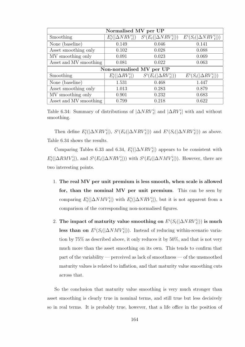
Normalised MV per UP
Smoothing Eit(|∆NRV i
t|) Si(Et(|∆NRV it|)) Ei(St(|∆NRV i
t|))None (baseline) 0.149 0.046 0.141Asset smoothing only 0.102 0.028 0.088MV smoothing only 0.091 0.023 0.069Asset and MV smoothing 0.081 0.022 0.063
Non-normalised MV per UP
Smoothing Eit(|∆RV i
t|) Si(Et(|∆RV it|)) Ei(St(|∆RV i
t|))None (baseline) 1.531 0.468 1.447Asset smoothing only 1.013 0.283 0.879MV smoothing only 0.901 0.232 0.683Asset and MV smoothing 0.799 0.218 0.622
Table 6.34: Summary of distributions of |∆NRV it| and |∆RV i
t| with and withoutsmoothing.
Then define Eit(|∆NRV i
t|), Si(Et(|∆NRV it|)) and Ei(St(|∆NRV i
t|)) as above.
Table 6.34 shows the results.
Comparing Tables 6.33 and 6.34, Eit(|∆NRV i
t|) appears to be consistent with
Eit(|∆RMV i
t|), and Si(Et(|∆NRV it|)) with Si(Et(|∆NMV i
t|)). However, there are
two interesting points.
1. The real MV per unit premium is less smooth, when scale is allowed
for, than the nominal MV per unit premium. This can be seen by
comparing Eit(|∆NMV i
t|) with Eit(|∆NRV i
t|), but it is not apparent from a
comparison of the corresponding non-normalised figures.
2. The impact of maturity value smoothing on Ei(St(|∆NRV it|)) is much
less than on Ei(St(|∆NMV it|)). Instead of reducing within-scenario varia-
tion by 75% as described above, it only reduces it by 50%, and that is not very
much more than the asset smoothing on its own. This tends to confirm that
part of the variability — perceived as lack of smoothness — of the unsmoothed
maturity values is related to inflation, and that maturity value smoothing cuts
across that.
So the conclusion that maturity value smoothing is very much stronger than
asset smoothing is clearly true in nominal terms, and still true but less decisively
so in real terms. It is probably true, however, that a life office in the position of
164
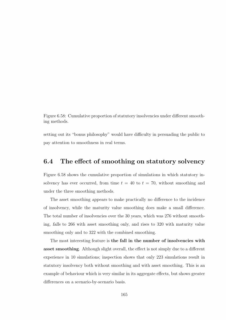
Figure 6.58: Cumulative proportion of statutory insolvencies under different smooth-ing methods.
setting out its “bonus philosophy” would have difficulty in persuading the public to
pay attention to smoothness in real terms.
6.4 The effect of smoothing on statutory solvency
Figure 6.58 shows the cumulative proportion of simulations in which statutory in-
solvency has ever occurred, from time t = 40 to t = 70, without smoothing and
under the three smoothing methods.
The asset smoothing appears to make practically no difference to the incidence
of insolvency, while the maturity value smoothing does make a small difference.
The total number of insolvencies over the 30 years, which was 276 without smooth-
ing, falls to 266 with asset smoothing only, and rises to 320 with maturity value
smoothing only and to 322 with the combined smoothing.
The most interesting feature is the fall in the number of insolvencies with
asset smoothing. Although slight overall, the effect is not simply due to a different
experience in 10 simulations; inspection shows that only 223 simulations result in
statutory insolvency both without smoothing and with asset smoothing. This is an
example of behaviour which is very similar in its aggregate effects, but shows greater
differences on a scenario-by-scenario basis.
165

6.5 The behaviour of the Bonus Smoothing Ac-
count
In this section we examine the behaviour of the BSA under different smoothing
schemes. It is helpful to start by setting out the properties which we would like the
BSA to possess.
1. The long-term cost of smoothing should be capable of being financed by the
normal operation of the smoothing method. That is, the BSA should ideally
tend to a stationary distribution.
2. The long term cost of smoothing should be reasonable in relation to the office’s
resources. We will be satisfied if the ratio BSA/AS is relatively small with
high probability.
3. Smoothing should contribute to the control of the cost of meeting the guaran-
tees, by absorbing as much as possible of that cost into the cost of smoothing.
This will be achieved if the ratio GCA/AS is significantly reduced by the
action of smoothing.
In addition, we should require of the smoothing method itself that it should
result in satisfactorily smoothed maturity values — a subjective matter — and that
it should not impair solvency.
6.5.1 The cost of guarantees without smoothing
In the absence of smoothing, and given that the maturity benefit is at least 100%
of the asset share, the BSA will be the same as the GCA and will represent the
accumulated cost of meeting the guarantees; that is, the accumulation of the differ-
ences between the asset shares of maturing policies and their guaranteed benefits,
in those years when the latter exceeded the former.
Figure 6.59 shows the distribution of the ratio BSA/AS in the absence of
smoothing. What is most interesting is how large (in magnitude) it can be; even at
the median level it approaches −0.2 — an accumulated cost of about 20% of the
166

Figure 6.59: 5th, 25th, 50th, 75th, 95th percentiles, and 10 sample paths, of theratio BSA/AS without smoothing.
asset shares, in other words — while the 5th quantile approaches −0.6. The need
to control this cost was discussed in Section 6.1 above.
6.5.2 The BSA with smoothing
Figures 6.60 – 6.62 show the distribution of the ratio BSA/AS under the three
different smoothing methods.
To what extent do these results satisfy our requirements?
1. The quantiles from the median downwards are all drifting slowly
down. For example, with asset smoothing only, there is a distinct downward
drift, more marked at the 5th quantile. In the later part of the period, the
75th quantile is approximately 0, so about 75% of offices have a negative BSA
at any time.
2. The ratio BSA/AS shows a marked tendency to spread out, with the
possible exception of positive ratios with asset smoothing only. The fact that
the 5th quantile is falling in all cases indicates a lack of long-term stability.
3. The ratio BSA/AS reaches large magnitudes with reasonably high
probability, especially in the presence of maturity value smoothing. From
167

Figure 6.60: 5th, 25th, 50th, 75th, 95th percentiles, and 10 sample paths, of theratio BSA/AS with asset smoothing only.
40 45 50 55 60 65 70
-1.0
-0.5
0.0
Figure 6.61: 5th, 25th, 50th, 75th, 95th percentiles, and 10 sample paths, of theratio BSA/AS with MV smoothing only.
168
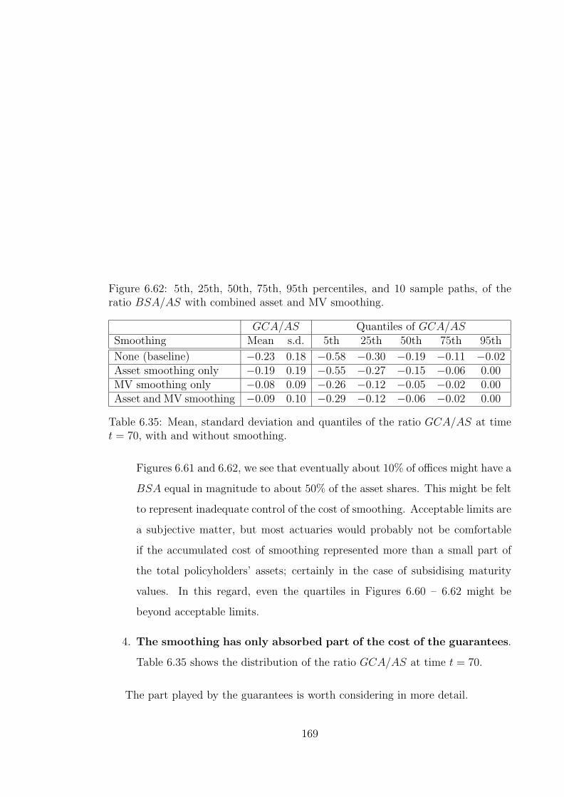
Figure 6.62: 5th, 25th, 50th, 75th, 95th percentiles, and 10 sample paths, of theratio BSA/AS with combined asset and MV smoothing.
GCA/AS Quantiles of GCA/ASSmoothing Mean s.d. 5th 25th 50th 75th 95th
None (baseline) −0.23 0.18 −0.58 −0.30 −0.19 −0.11 −0.02Asset smoothing only −0.19 0.19 −0.55 −0.27 −0.15 −0.06 0.00MV smoothing only −0.08 0.09 −0.26 −0.12 −0.05 −0.02 0.00Asset and MV smoothing −0.09 0.10 −0.29 −0.12 −0.06 −0.02 0.00
Table 6.35: Mean, standard deviation and quantiles of the ratio GCA/AS at timet = 70, with and without smoothing.
Figures 6.61 and 6.62, we see that eventually about 10% of offices might have a
BSA equal in magnitude to about 50% of the asset shares. This might be felt
to represent inadequate control of the cost of smoothing. Acceptable limits are
a subjective matter, but most actuaries would probably not be comfortable
if the accumulated cost of smoothing represented more than a small part of
the total policyholders’ assets; certainly in the case of subsidising maturity
values. In this regard, even the quartiles in Figures 6.60 – 6.62 might be
beyond acceptable limits.
4. The smoothing has only absorbed part of the cost of the guarantees.
Table 6.35 shows the distribution of the ratio GCA/AS at time t = 70.
The part played by the guarantees is worth considering in more detail.
169

The asset smoothing on its own absorbs only a small part of the cost of the
guarantees, and the standard deviation of the ratio GCA/AS is slightly higher. The
maturity value smoothing absorbs a much larger part of the cost of guarantees, and
reduces considerable the dispersion of the GCA. This explains the greater downward
drift of the 5th quantile when there is maturity value smoothing. Intuitively, on
those occasions when a large fall in the value of the assets reduces the value of the
asset shares suddenly, the asset smoothing on its own, being the weaker method,
will more often allow the calculated maturity value to fall below the level of the
guarantees; when this happens, the cost of meeting the guarantee falls on the GCA.
However, the stronger maturity value smoothing may prevent or delay the smoothed
maturity values from falling below the level of the guarantees, and in this case so
the cost of subsidising maturity values falls on the BSA rather than on the GCA.
The example in Table 6.32 shows what is happening.
This feature is illustrated by Figure 6.63, which shows the number of simulations
at each time during the projection period for which the calculated rate of terminal
bonus was negative. This is the same as the number of simulations in which the
guarantees exceeded the calculated maturity value. The fact that over 25% of the
offices are meeting guarantees at any time is itself interesting. The figure shows
that asset smoothing has little effect, but that maturity value smoothing reduces by
about one-third the incidence of negative terminal bonus.
Maturity value smoothing is much more effective than asset smoothing. It also
absorbs a much larger part of the cost of the guarantees, which would be desirable
if the cost of smoothing itself was bounded, but this does not appear to be the case.
None of the smoothing methods meet our criteria for the reasonable behaviour of
the BSA. Asset smoothing on its own is perhaps closest.
In the next sections we will consider ways in which the instability of the long
term cost of smoothing might be controlled, with emphasis on the probability of
large negative values of the BSA.
170

Figure 6.63: No. of simulations with negative theoretical terminal bonus, with andwithout smoothing.
6.5.3 The effect of new business growth
Section 6.1 described how a life office’s additional estate — even if negative — might
be eliminated in relative terms by new business growth. The same is true of the
BSA. The higher the rate of new business growth, the smaller the increments to
the BSA relative to the in-force asset shares, and the smaller the changes in the
ratio BSA/AS.
In the baseline office the rate of new business growth is equal to the rate of
price inflation. Figures 6.64 and 6.65 show the effect on the distribution of the
ratio BSA/AS of new business growth 5% and 10% greater than the rate of price
inflation, respectively. In both cases the combined smoothing algorithm is used, so
these should be compared with Figure 6.62.
Given the parameters we have used for the Wilkie model, 5% real new business
growth represents a mean rate a little above the mean rate of return on the assets.
A high rate of new business growth quite effectively limits the growth of the
BSA/AS ratio. However, new business growth cannot sensibly be viewed as a
means towards that end. Growth, if attainable, would be aimed at for other reasons;
it is not likely that containment of the cost of smoothing would or should dictate
new business policy. In particular, the consequences of suffering lower rates of new
171

Figure 6.64: 5th, 25th, 50th, 75th, 95th percentiles, and 10 sample paths, of theratio BSA/AS with 5% real new business growth.
40 45 50 55 60 65 70
-1.0
-0.5
0.0
Figure 6.65: 5th, 25th, 50th, 75th, 95th percentiles, and 10 sample paths, of theratio BSA/AS with 10% real new business growth.
172

Figure 6.66: 5th, 25th, 50th, 75th, 95th percentiles, and 10 sample paths, of theratio BSA/AS with −5% real new business growth.
business growth, or even closure, might be serious. Figure 6.66 shows the effect of
−5% real new business growth.
The benefits of high new business growth can quickly be lost if that rate of
growth cannot be sustained. The simple forms of smoothing which we have used
are not sufficiently self-regulating in these circumstances. Therefore other means of
controlling the ratio BSA/AS should be investigated.
6.5.4 Feedback from the BSA
A possible approach to the control of the BSA/AS ratio is to bring it into the
smoothing algorithm. If the ratio stands at a high level, maturity values could
be increased to bring it down — or at least to prevent it from rising further —
while if it reaches a low level, maturity values could be cut to bring it back up. A
simple method is to multiply the calculated maturity value by the factor (called the
“feedback factor”)
1 +BSA
AS
at some stage in the smoothing process. In the model, this was carried out before
the limits on the annual changes in maturity values were applied, and naturally
173

Figure 6.67: 5th, 25th, 50th, 75th, 95th percentiles, and 10 sample paths, of theratio BSA/AS with feedback and asset smoothing only.
before the calculated maturity value was checked against the guarantees. In other
words, feedback was applied between the steps 1 and 2 described in Section 6.2.1. It
is arguable that feedback should come in after step 2, since otherwise the effect might
be to put feedback into the maturity value and then, by applying the smoothing
rule 2, to take it out again. On the other hand, to bring in feedback after all
the smoothing rules have been applied might be felt to negate the very purpose of
smoothing.
Figures 6.67 — 6.69 show the effect of this feedback in conjunction with asset
smoothing, maturity value smoothing and combined smoothing respectively.
1. Comparing Figure 6.67 with Figure 6.60 (asset smoothing only), it is evident
that the feedback is only partially effective. It reduces the ratio BSA/AS
acceptably for positive values, but it has little effect on the downward drift of
the 5th quantile. It is interesting to note, again, that the number of statutory
insolvencies falls slightly further, to 263 (from 266 with no feedback), but that
only 232 of these cases also give rise to insolvency if there is no feedback,
and only 226 if there is no smoothing at all. In all 332 scenarios give rise
to insolvency under at least one of these three strategies. It is misleading to
assume that a modest change in the number of insolvencies implies modest
174

Figure 6.68: 5th, 25th, 50th, 75th, 95th percentiles, and 10 sample paths, of theratio BSA/AS with feedback and MV smoothing only.
40 45 50 55 60 65 70
-1.0
-0.5
0.0
Figure 6.69: 5th, 25th, 50th, 75th, 95th percentiles, and 10 sample paths, of theratio BSA/AS with feedback and combined asset and MV smoothing.
175

GCA/AS Quantiles of GCA/ASSmoothing Mean s.d. 5th 25th 50th 75th 95th
None (baseline) −0.23 0.18 −0.58 −0.30 −0.19 −0.11 −0.02
Without feedbackAsset smoothing only −0.19 0.19 −0.55 −0.27 −0.15 −0.06 0.00MV smoothing only −0.08 0.09 −0.26 −0.12 −0.05 −0.02 0.00Asset and MV smoothing −0.09 0.10 −0.29 −0.12 −0.06 −0.02 0.00
With feedbackAsset smoothing only −0.43 0.47 -1.23 −0.58 −0.30 −0.13 −0.01MV smoothing only −0.26 −0.37 −0.77 −0.34 −0.16 −0.05 0.00Asset and MV smoothing −0.27 0.38 −0.80 −0.35 −0.17 −0.05 0.00
Table 6.36: Mean, standard deviation and quantiles of the ratio GCA/AS at timet = 70, with and without feedback from the ratio BSA/AS.
changes within each scenario.
2. Comparing Figure 6.68 with Figure 6.61 (maturity value smoothing only),
again the distribution is compressed for positive values of the ratio, but not
for negative values.
3. Comparing Figure 6.69 with Figure 6.62 (combined smoothing), the ratio is
slightly more dispersed than before below the median.
4. It is also noticeable — especially in Figures 6.69 and 6.62 — that the sample
paths are not always closer to zero in the presence of feedback.
The explanation for the failure to control negative values of the ratio BSA/AS
lies in the operation of the guarantees. If the guarantees are called upon when
the BSA is negative, then the office will be unable to reduce the maturity value
by applying the feedback factor. No such restriction will apply when the BSA is
positive, so the feedback will be slightly out of balance.
Table 6.36 shows the distribution of the ratio GCA/AS, without smoothing,
with smoothing but without feedback, and with both smoothing and feedback (the
first two are reproduced from Table 6.35 for convenience).
Feedback has not only increased the cost of the guarantees, compared
with the smoothing methods without feedback: it has also increased it
compared with the unsmoothed case. More precisely, the distribution of the
176
Figure 6.70: No. of simulations with negative theoretical terminal bonus, with andwithout smoothing, in the presence of feedback.
ratio GCA/AS is more dispersed in the presence of feedback, and the lower quantiles
are significantly reduced, while the upper quantiles are only slightly increased. In
other words, the “worst cases” are worse with feedback than without feedback,
or even without smoothing. Figure 6.70 shows the incidence of negative terminal
bonus rates when feedback is used. They are larger even than those arising with no
smoothing.
It is worth looking in more detail at the ratio BSA/AS with and without feed-
back. Figure 6.71 shows the distribution, during the whole period t = 40 to t = 70,
of those 100 sample paths which comprised the bottom decile of the distribution of
the ratio BSA/AS at time t = 55, assuming combined smoothing and no feedback.
Figure 6.72 shows the corresponding distribution of those sample paths comprising
the top decile at t = 55.
There is a qualitative difference between the behaviour of the ratio BSA/AS
above and below zero. There is much greater volatility of positive values of the
ratio. In neither case is there any strong tendency for the ratio to revert to zero.
This does not satisfy our intuitive wish for smoothing to be cost-neutral over time.
Figures 6.73 and 6.74 show the corresponding distributions with combined smooth-
ing and feedback.
The effect of the feedback on positive values of the BSA is clear. In fact by time
177

Figure 6.71: 5th, 25th, 50th, 75th, 95th percentiles, and 10 sample paths, of theratio BSA/AS given in the bottom decile at t = 55.
40 45 50 55 60 65 70
-1.0
-0.5
0.0
Figure 6.72: 5th, 25th, 50th, 75th, 95th percentiles, and 10 sample paths, of theratio BSA/AS given in the top decile at t = 55.
178

Figure 6.73: 5th, 25th, 50th, 75th, 95th percentiles, and 10 sample paths, of theratio BSA/AS with feedback given in the bottom decile at t = 55.
40 45 50 55 60 65 70
-1.0
-0.5
0.0
Figure 6.74: 5th, 25th, 50th, 75th, 95th percentiles, and 10 sample paths, of theratio BSA/AS with feedback given in the top decile at t = 55.
179
Figure 6.75: 5th, 25th, 50th, 75th, 95th percentiles, and 10 sample paths, of theratio BSA/AS with smoothing given negative terminal bonus at t = 55.
t = 70 more than 75% of these cases have negative BSAs, which certainly indicates
a reversion towards zero. The same tendency exists, but much less strongly, when
the BSA is negative. The reason is, as mentioned above, that the full feedback
factor cannot be applied to reduce the maturity payment if the guarantees have
been uncovered. The force of this can be gauged from Figure 6.75, which shows
the distribution of the ratio BSA/AS for those simulations in which the guarantees
were uncovered at time t = 55, assuming combined smoothing and feedback. (There
were 310 such cases.)
In other words, in 310 simulations the calculated maturity values (after smooth-
ing) of policies maturing at t = 55 were less than the guaranteed benefits. This is
indicated by a negative theoretical terminal bonus at that time, which is how it is
described in the figure. The figure shows that, at time t = 54, the BSA in these
simulations was almost always negative. Therefore the BSA at time t = 55 will
also be negative before the calculation of maturity values (BSAs shown here are
after the payment of claims) and the feedback factor will be less than 1. However,
the imposition of the guarantees means that the feedback factor is wholly or partly
ineffective.
Table 6.37 summarises the effect on benefits of smoothing with and without
feedback. (The figures without smoothing and without feedback are reproduced
180

Normalised MV per UP
Smoothing Eit(|∆NMV i
t|) Si(Et(|∆NMV it|)) Ei(St(|∆NMV i
t|))No smoothingNone (baseline) 0.136 0.049 0.145
Without feedbackAsset smoothing only 0.087 0.032 0.087MV smoothing only 0.073 0.019 0.038Asset and MV smoothing 0.065 0.019 0.040
With feedbackAsset smoothing only 0.095 0.037 0.102MV smoothing only 0.071 0.023 0.043Asset and MV smoothing 0.067 0.023 0.043
Normalised real MV per UP
Smoothing Eit(|∆NRV i
t|) Si(Et(|∆NRV it|)) Ei(St(|∆NRV i
t|))No smoothingNone (baseline) 0.149 0.046 0.141
Without feedbackAsset smoothing only 0.102 0.028 0.088MV smoothing only 0.091 0.023 0.069Asset and MV smoothing 0.081 0.022 0.063
With feedbackAsset smoothing only 0.111 0.033 0.102MV smoothing only 0.091 0.027 0.071Asset and MV smoothing 0.085 0.026 0.068
Table 6.37: Summary of distributions of |∆NMV it| and |∆NRV i
t| with and withoutfeedback.
from Tables 6.33 and 6.34 for convenience.)
Feedback has little effect on the overall smoothness if maturity value smoothing
is used, not surprisingly since the smoothing is applied after the feedback. It has
a greater effect under asset smoothing alone, increasing both Eit(|∆NMV i
t|) and
Ei(St(|∆NMV it|)) and the corresponding “real” measures. It is intuitively clear
that if feedback counters the effect of smoothing on the BSA, it should reduce the
smoothness. Table 6.37 suggests that it does so moderately. Figure 6.76 (compare
with Figure 6.52) confirms that the smoothing is not much less effective than it is
without feedback.
The effect of feedback on statutory solvency is shown in Table 6.38.
The most interesting aspect of this qualitative discussion of the behaviour of the
ratio BSA/AS is the apparent difficulty of applying maturity value smoothing in a
181

Figure 6.76: 5th, 25th, 50th, 75th, 95th percentiles, and 10 sample paths, of thedifference ∆MV a
t with asset smoothing only and feedback.
No. of statutory insolvenciesNo feedback With feedback
Asset smoothing only 266 263MV smoothing only 320 389Asset and MV smoothing 322 423
Table 6.38: Effect of feedback on statutory insolvency between t = 40 and t = 55.
182
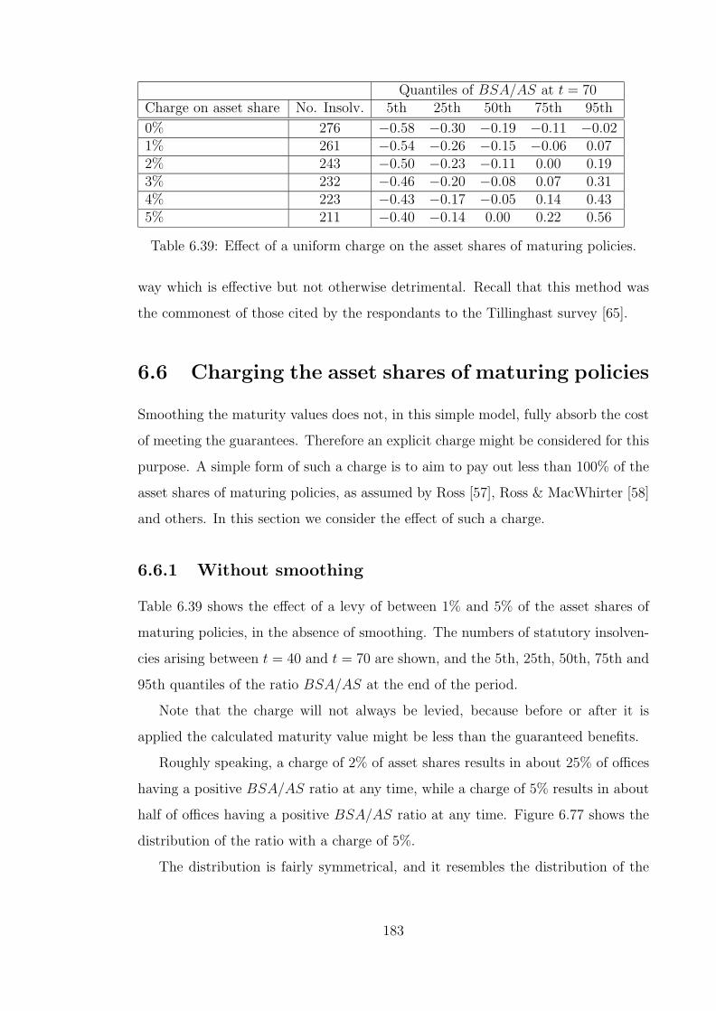
Quantiles of BSA/AS at t = 70Charge on asset share No. Insolv. 5th 25th 50th 75th 95th
0% 276 −0.58 −0.30 −0.19 −0.11 −0.021% 261 −0.54 −0.26 −0.15 −0.06 0.072% 243 −0.50 −0.23 −0.11 0.00 0.193% 232 −0.46 −0.20 −0.08 0.07 0.314% 223 −0.43 −0.17 −0.05 0.14 0.435% 211 −0.40 −0.14 0.00 0.22 0.56
Table 6.39: Effect of a uniform charge on the asset shares of maturing policies.
way which is effective but not otherwise detrimental. Recall that this method was
the commonest of those cited by the respondants to the Tillinghast survey [65].
6.6 Charging the asset shares of maturing policies
Smoothing the maturity values does not, in this simple model, fully absorb the cost
of meeting the guarantees. Therefore an explicit charge might be considered for this
purpose. A simple form of such a charge is to aim to pay out less than 100% of the
asset shares of maturing policies, as assumed by Ross [57], Ross & MacWhirter [58]
and others. In this section we consider the effect of such a charge.
6.6.1 Without smoothing
Table 6.39 shows the effect of a levy of between 1% and 5% of the asset shares of
maturing policies, in the absence of smoothing. The numbers of statutory insolven-
cies arising between t = 40 and t = 70 are shown, and the 5th, 25th, 50th, 75th and
95th quantiles of the ratio BSA/AS at the end of the period.
Note that the charge will not always be levied, because before or after it is
applied the calculated maturity value might be less than the guaranteed benefits.
Roughly speaking, a charge of 2% of asset shares results in about 25% of offices
having a positive BSA/AS ratio at any time, while a charge of 5% results in about
half of offices having a positive BSA/AS ratio at any time. Figure 6.77 shows the
distribution of the ratio with a charge of 5%.
The distribution is fairly symmetrical, and it resembles the distribution of the
183
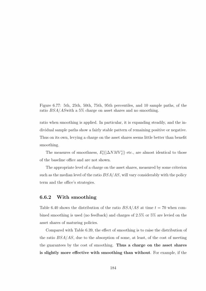
Figure 6.77: 5th, 25th, 50th, 75th, 95th percentiles, and 10 sample paths, of theratio BSA/ASwith a 5% charge on asset shares and no smoothing.
ratio when smoothing is applied. In particular, it is expanding steadily, and the in-
dividual sample paths show a fairly stable pattern of remaining positive or negative.
Thus on its own, levying a charge on the asset shares seems little better than benefit
smoothing.
The measures of smoothness, Eit(|∆NMV i
t|) etc., are almost identical to those
of the baseline office and are not shown.
The appropriate level of a charge on the asset shares, measured by some criterion
such as the median level of the ratio BSA/AS, will vary considerably with the policy
term and the office’s strategies.
6.6.2 With smoothing
Table 6.40 shows the distribution of the ratio BSA/AS at time t = 70 when com-
bined smoothing is used (no feedback) and charges of 2.5% or 5% are levied on the
asset shares of maturing policies.
Compared with Table 6.39, the effect of smoothing is to raise the distribution of
the ratio BSA/AS, due to the absorption of some, at least, of the cost of meeting
the guarantees by the cost of smoothing. Thus a charge on the asset shares
is slightly more effective with smoothing than without. For example, if the
184
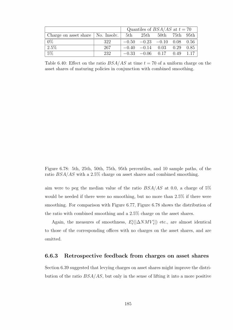
Quantiles of BSA/AS at t = 70Charge on asset share No. Insolv. 5th 25th 50th 75th 95th
0% 322 −0.50 −0.23 −0.10 0.08 0.562.5% 267 −0.40 −0.14 0.03 0.29 0.855% 232 −0.33 −0.06 0.17 0.49 1.17
Table 6.40: Effect on the ratio BSA/AS at time t = 70 of a uniform charge on theasset shares of maturing policies in conjunction with combined smoothing.
Figure 6.78: 5th, 25th, 50th, 75th, 95th percentiles, and 10 sample paths, of theratio BSA/AS with a 2.5% charge on asset shares and combined smoothing.
aim were to peg the median value of the ratio BSA/AS at 0.0, a charge of 5%
would be needed if there were no smoothing, but no more than 2.5% if there were
smoothing. For comparison with Figure 6.77, Figure 6.78 shows the distribution of
the ratio with combined smoothing and a 2.5% charge on the asset shares.
Again, the measures of smoothness, Eit(|∆NMV i
t|) etc., are almost identical
to those of the corresponding offices with no charges on the asset shares, and are
omitted.
6.6.3 Retrospective feedback from charges on asset shares
Section 6.39 suggested that levying charges on asset shares might improve the distri-
bution of the ratio BSA/AS, but only in the sense of lifting it into a more positive
185

Figure 6.79: 5th, 25th, 50th, 75th, 95th percentiles, and 10 sample paths, of theratio BSA/AS with a 10% charge on asset shares, feedback and no smoothing.
region. The dispersion of the ratio was little changed, which meant that the possi-
bility of large negative values was only avoided by accepting large positive values.
This was true even in the presence of feedback from the ratio BSA/AS. This seems
to be rather a blunt instrument.
An alternative is to levy a large enough charge on the asset shares to satisfy the
needs of solvency and stability below the line (if possible), and to apply feedback so
that the excess charges (which will be the rule) are returned retrospectively to the
policyholders. Not, admittedly, to the same policyholders who provided them, but
it is arguable that this is an inevitable consequence of pooling investment risks.
Figure 6.79 shows the effect of a charge of 10% of the asset shares of matur-
ing policies, combined with feedback but with no smoothing. There are several
interesting points.
1. The figure shows satisfactory stability in its upper range, appearing to level
out and not spreading noticeably.
2. In its lower range the distribution continues to disperse.
However, the combination of charges plus feedback results in maturity values
which progress no more smoothly than those with no smoothing or charges at all.
186

Quantiles of BSA/AS at t = 70Charge on asset shares No. Insolv. 5th 25th 50th 75th 95th
No smoothing5% charge 222 −0.37 −0.10 0.00 0.05 0.0710% charge 205 −0.33 −0.06 0.05 0.12 0.17
Combined smoothing5% charge 366 −0.59 −0.18 −0.02 0.11 0.4510% charge 309 −0.54 −0.13 0.05 0.20 0.58
Table 6.41: Effect on statutory solvency and on the ratio BSA/AS at time t = 70of feedback in conjunction with charges on asset shares.
The various measures of smoothness Eit(|∆NMV i
t|) etc., are almost identical to
those of the corresponding offices without charges on the asset shares and are not
shown.
For comparison, Table 6.41 also shows the effect of using combined smoothing
in conjunction with charges on the asset shares and feedback.
6.7 Restrictions on feedback
The examples of feedback in Section 6.5.4 assumed that the benefits were to be
enhanced whenever the ratio BSA/AS was positive, and reduced whenever it was
negative. This was in accord with the idea of “cost neutral” smoothing. However,
the results were less than satisfactory both as regards statutory solvency and the
stability of the cost of smoothing.
It might be considered unreasonable, in view of the potential instability of the
BSA, to attempt to control it around a mean level of BSA = 0. It might instead be
reasonable to allow the ratio BSA/AS to rise to some positive level before applying
feedback. In this section we consider that and one other possibility.
Delayed feedback The feedback algorithm applies the feedback factor
1 +BSA
AS
to the calculated maturity value, before applying the limits on the changes in
maturity values. It does so whatever the value of the ratio BSA/AS. Thus,
187

benefits are enhanced when the ratio is positive, no matter how small. We will
call this “full feedback”.
Instead we might delay the application of feedback until the ratio had reached
some positive level, so that the BSA might have a more favourable distri-
bution, especially at the bottom end. We will call this “delayed feedback”,
although the “delay” involved is not temporal. Of course, feedback is still
applied whenever the ratio is negative. For example, with a threshold of 0.1,
we would apply feedback when the ratio BSA/AS was below 0 or above 0.1,
but not in between.
Offset feedback We might expect to be too late if we wait for the BSA to become
negative before reducing the calculated benefits; that could mean that too
often the reduction cannot be effected because of the guarantees. In addition,
a threshold of 0.1 or 0.2 (for example) means that in some circumstances a
small change in conditions between one year and the next will result in a jump
of 10% or 20% in the benefits, which is possibly inequitable (and certainly not
smooth).
Therefore we might consider moderating feedback by offsetting the ratio used
to calculate the feedback factor. For example, with an offset of 0.1, we would
apply the factor
0.9 +BSA
AS
so that calculated benefits would be reduced when the ratio BSA/AS was
below 1.1, and enhanced above that level.
Note that offsetting the feedback factor is effectively imposing a charge on the
asset shares of maturing policies, so it has a lot in common with the charging
strategies of Section 6.6.3.
Inspection shows that the visible effect on smoothing is small (and the measures
Eit(|∆NMV i
t|) etc. are almost identical to those of the corresponding office with
full feedback) so we will not show any figures, but Table 6.42 shows the effect on
the distribution of the ratio BSA/AS at time t = 70 of:
188

Quantiles of BSA/AS at t = 70Limits on feedback No. Insolv. 5th 25th 50th 75th 95th
Full feedbackBSA/AS < 0 or > 0.0 423 −0.64 −0.22 −0.07 0.04 0.34
Modified feedbackBSA/AS < 0 or > 0.1 405 −0.64 −0.21 −0.05 0.06 0.37BSA/AS < 0 or > 0.2 361 −0.59 −0.17 −0.03 0.10 0.41BSA/AS offset by 0.1 319 −0.57 −0.15 0.04 0.18 0.56BSA/AS offset by 0.1 and off-set BSA/AS < 0 or > 0.1
304 −0.55 −0.13 0.05 0.19 0.57
Table 6.42: Effect on statutory solvency and on the ratio BSA/AS at time t = 70of modified feedback, with combined smoothing.
GCA/AS Quantiles of GCA/ASLimits on feedback Mean s.d. 5th 25th 50th 75th 95th
Full feedbackNone (baseline) −0.27 0.38 −0.80 −0.35 −0.17 −0.05 0.00
Modified feedbackBSA/AS < 0 or > 0.1 −0.26 0.38 −0.78 −0.33 −0.16 −0.05 0.00BSA/AS < 0 or > 0.2 −0.26 0.39 −0.78 −0.33 −0.16 −0.04 0.00BSA/AS offset by 0.1 −0.33 0.41 −1.00 −0.47 −0.23 −0.06 0.00BSA/AS offset by 0.1 and off-set BSA/AS < 0 or > 0.1
−0.33 0.41 −0.97 −0.47 −0.23 −0.06 0.00
Table 6.43: Mean, standard deviation and quantiles of the ratio GCA/AS at timet = 70, with combined smoothing and modified feedback.
1. delaying feedback until the ratio reaches 0.1;
2. delaying feedback until the ratio reaches 0.2;
3. offsetting the ratio BSA/AS by 0.1 as described above;
4. offsetting the ratio BSA/AS by 0.1 as described above and applying feedback
only when the offset ratio is less than 0 or greater than 0.1 (a combination of
delayed and offset feedback).
Table 6.43 shows the distribution of the ratio GCA/AS at time t = 70.
Comparing these four strategies, we see that they have similar effects but to
different degrees.
1. They all improve statutory solvency. All these strategies retain assets which
are used to subsidise maturity payments under the full feedback. Therefore
189

the statutory solvency should be improved, although this is not certain be-
cause there might be second order effects arising from the asset allocation.
Offset feedback retains more assets in the BSA than delayed feedback, with a
correspondingly larger improvement in solvency.
2. The distribution of the ratio BSA/AS is improved. Offset feedback is more
effective than delayed feedback, for the same reasons as above, but what is most
interesting is that the improvements are small at the 5th and 25th quantiles.
3. Under delayed feedback, the distribution of the ratio GCA/AS is improved,
but by a negligible amount. Under offset feedback, the distribution of the
ratio GCA/AS is lower than it is with full feedback. At first sight this is
surprising, but it has a simple explanation. Applying a feedback factor of less
than 1.0 increases the chances of uncovering the guarantees; whenever this
happens, the GCA is called upon to subsidise the benefits. Offset feedback
decreases all feedback factors, while delayed feedback only decreases those
between the specified limits, so the depletion of the GCA will be greater under
offset feedback — in effect it is absorbed less into the cost of smoothing.
The extent to which guarantees are uncovered more often with modified feed-
back can be gauged from Table 6.44. This shows the numbers of simulations
with full feedback and with modified feedback under which the stated negative
theoretical terminal bonus rates were ever attained. (Recall that a negative
theoretical terminal bonus rate is equivalent to the uncovering of the guar-
antees.) The table shows that offset feedback encounters theoretical terminal
bonus rates in the range −20% – −30% much more frequently. Inspection
also shows that at most times more offices have negative terminal bonus under
offset feedback than under full feedback.
None of these modifications of full feedback have remedied, to any extent, the
defects of smoothing with or without feedback. However, Table 6.43 in particular
shows where the problem lies; attempts to reduce maturity values to control the cost
of smoothing simply transfer the adverse experience from the BSA to the GCA.
A further observation is that such methods as we have studied make the processes
190

Theoretical Terminal BonusLimits on feedback 0% -10% -20% -30% -40% -50%
Full feedbackNone (baseline) 933 777 488 178 71 37
Modified feedbackBSA/AS < 0 or > 0.1 920 764 461 165 67 38BSA/AS < 0 or > 0.2 911 748 447 159 59 33BSA/AS offset by 0.1 924 790 593 281 87 42BSA/AS offset by 0.1 and off-set BSA/AS < 0 or > 0.1
919 778 585 273 87 42
Table 6.44: Numbers of simulations in which the theoretical terminal bonus ratesever fell below the levels shown.
of granting guarantees — that is, setting premium rates and declaring reversionary
bonuses — and the process of charging for guarantees quite separate. Guarantees
are granted prospectively, to be paid for retrospectively. Such an approach is con-
sistent with recent practice in the U.K. (see Chapter 1) but here it seems to lead to
difficulties.
6.8 How robust is the cost of smoothing?
The whole idea of with-profits business smoothing out the peaks and troughs of the
stock market depends on the stock market behaving in that way. Any smoothing
strategy is vulnerable to changes in conditions which do not conform to the expected
pattern. For example, what happens if a life office subsidises maturity payments
during a downswing which turns out to be a permanent reduction in rates of return?
In this section we look at a few possibilities.
In addition to perverse behaviour of the investment markets (or perhaps be-
haviour not in line with perverse expectations!) a smoothing strategy might not
give exactly the expected results because of the practicalities of implementing it.
For example, if assets are smoothed, what happens if the smoothed values are bi-
ased? We also consider some of these aspects.
In this section, the combined smoothing algorithm with no feedback was used
unless otherwise stated.
191

6.8.1 Robustness to changes in financial conditions
The results given so far show that the Wilkie asset model provides financial con-
ditions which permit asset smoothing and maturity value smoothing which, if not
stable, are at least not biased to any significant extent. However, the Wilkie model
posits a stable underlying structure of first and second moments of the quantities
modelled. This means, for example, that the force of inflation always reverts to the
same mean, and always suffers random shocks with the same variance.
It is arguable that large-scale or persistent changes in financial conditions do
not fit into this framework, and that they might instead be modelled by assuming
that the underlying structure of (say) first and second moments can change from
time to time. In between such changes, a Wilkie-type model might be assumed to
be adequate. Although such time series models are well known (see, for example,
Geoghegan et al [26]) they have not been applied for actuarial use.
They do, however, suggest a simple method of investigating a given shift in fi-
nancial conditions, by changing parameters in the Wilkie model. A simple example
would be to change the parameter QMU , which represents the mean force of infla-
tion, from 0.05 to 0.25 (say) to represent a move to a more inflationary economy.
Three questions about such changes are:
1. How long does it take the smoothing algorithm to catch up with a permanent
shift in conditions?
2. How long does it take the smoothing algorithm to bounce back from a tempo-
rary but large scale shift in conditions?
3. What is the potential for losses (or profits) before the smoothing algorithm
does catch up?
Some more simple minded smoothing algorithms — for example, smoothing the
assets by discounting future income at a fixed yield — would never catch up. On this
ground alone, any such method is bound to up-date the assumptions dynamically
in some way. The 5-year moving average yields which we have used, even if they
ought not to be regarded as estimates of mean future yields, do at least keep the
office in touch with changes in the general level of yields.
192

Figure 6.80: 5th, 25th, 50th, 75th, 95th percentiles, and 10 sample paths, of theratio BSA/AS, Y MU = 0.05 from t = 40.
We experimented with permanent shifts in the model parameters representing
mean values, namely
QMU the mean force of inflation
Y MU the mean gross dividend yield
DMU the mean real rate of dividend growth
CMU the mean real gross gilt yield
Of these, only changes in Y MU had significant effects. The pattern of BSA/AS
ratios was little affected by (moderate) changes in the others. This is interesting
in the case of inflation, since that influences all the other elements of the Wilkie
model, but perhaps should not be surprising. The influence of inflation on other
variables is exponentially lagged in the Wilkie model, which itself imparts an element
of smoothing, and the influence of the limits on annual changes in relative maturity
values might still predominate in the smoothing algorithm itself. CMU had limited
influence anyway, since the level of gilt investment in the model was low.
Figure 6.80 shows the effect on the BSA/AS ratio of a change in the mean gross
dividend yield Y MU at time t = 40, from 0.04 to 0.05.
193
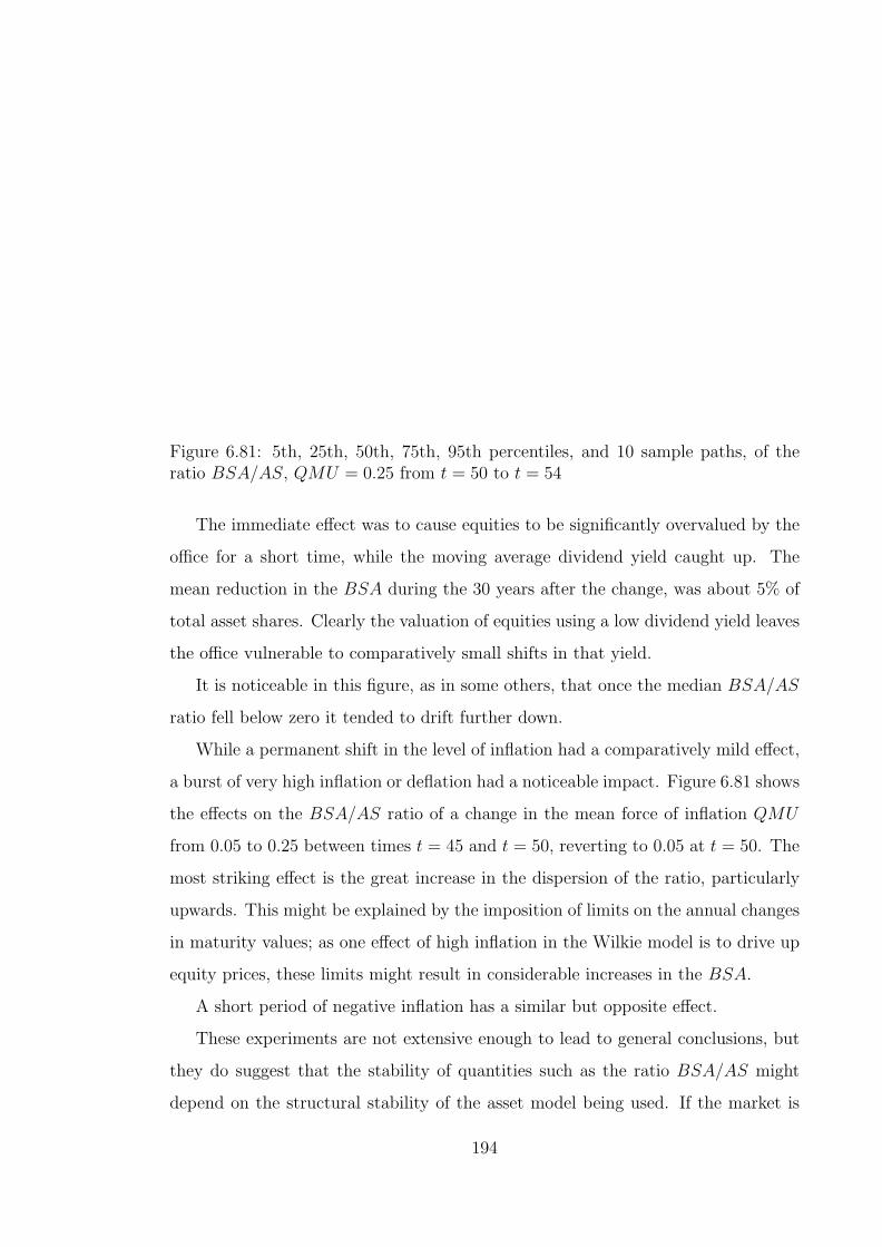
Figure 6.81: 5th, 25th, 50th, 75th, 95th percentiles, and 10 sample paths, of theratio BSA/AS, QMU = 0.25 from t = 50 to t = 54
The immediate effect was to cause equities to be significantly overvalued by the
office for a short time, while the moving average dividend yield caught up. The
mean reduction in the BSA during the 30 years after the change, was about 5% of
total asset shares. Clearly the valuation of equities using a low dividend yield leaves
the office vulnerable to comparatively small shifts in that yield.
It is noticeable in this figure, as in some others, that once the median BSA/AS
ratio fell below zero it tended to drift further down.
While a permanent shift in the level of inflation had a comparatively mild effect,
a burst of very high inflation or deflation had a noticeable impact. Figure 6.81 shows
the effects on the BSA/AS ratio of a change in the mean force of inflation QMU
from 0.05 to 0.25 between times t = 45 and t = 50, reverting to 0.05 at t = 50. The
most striking effect is the great increase in the dispersion of the ratio, particularly
upwards. This might be explained by the imposition of limits on the annual changes
in maturity values; as one effect of high inflation in the Wilkie model is to drive up
equity prices, these limits might result in considerable increases in the BSA.
A short period of negative inflation has a similar but opposite effect.
These experiments are not extensive enough to lead to general conclusions, but
they do suggest that the stability of quantities such as the ratio BSA/AS might
depend on the structural stability of the asset model being used. If the market is
194
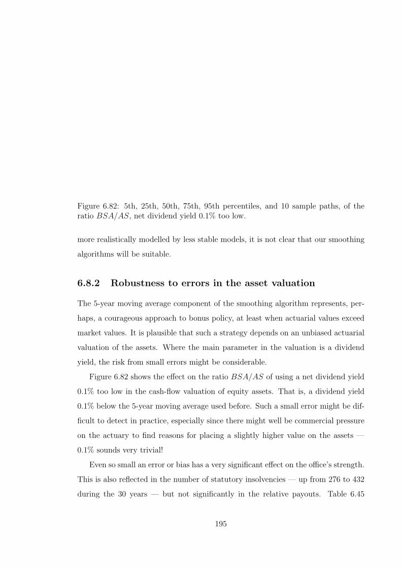
Figure 6.82: 5th, 25th, 50th, 75th, 95th percentiles, and 10 sample paths, of theratio BSA/AS, net dividend yield 0.1% too low.
more realistically modelled by less stable models, it is not clear that our smoothing
algorithms will be suitable.
6.8.2 Robustness to errors in the asset valuation
The 5-year moving average component of the smoothing algorithm represents, per-
haps, a courageous approach to bonus policy, at least when actuarial values exceed
market values. It is plausible that such a strategy depends on an unbiased actuarial
valuation of the assets. Where the main parameter in the valuation is a dividend
yield, the risk from small errors might be considerable.
Figure 6.82 shows the effect on the ratio BSA/AS of using a net dividend yield
0.1% too low in the cash-flow valuation of equity assets. That is, a dividend yield
0.1% below the 5-year moving average used before. Such a small error might be dif-
ficult to detect in practice, especially since there might well be commercial pressure
on the actuary to find reasons for placing a slightly higher value on the assets —
0.1% sounds very trivial!
Even so small an error or bias has a very significant effect on the office’s strength.
This is also reflected in the number of statutory insolvencies — up from 276 to 432
during the 30 years — but not significantly in the relative payouts. Table 6.45
195

Mean MV per UP deflated Mean payout ratioSmoothing Mean s.d. Mean s.d.
None (baseline) 10.264 1.716 1.000 0.000
Asset valn. yield 0.1% toolow
9.910 1.665 0.990 0.040
Asset valn. yield 0.2% toolow
9.973 1.681 0.998 0.050
Table 6.45: Comparison of maturity values deflated by Retail Price Inflation, andpayout ratios with respect to the baseline projection.
summarises the effect on benefits of the perturbations described here. The first two
columns show the means and standard deviations of the mean maturity value per
unit premium in each simulation, deflated to allow for inflation. The last pair of
columns show the mean and standard deviation of the mean values of the ratios
MV ct
MV tin each simulation.
These figures suggest that smoothing methods might sometimes be sensitive to
the assumptions, and lead to errors whose detection would not be easy.
6.9 Conclusions
1. The relative cost of smoothing (measured by the ratio BSA/AS) is not nec-
essarily stable over time; the accumulated historic costs of smoothing can be
considerable.
2. The smoothing of maturity values appeared to be more effective than the
smoothing of asset values, and absorbed a larger part of the cost of the guar-
antees, but the accumulated cost of smoothing was considerably less stable.
3. The rate of new business growth has a considerable impact on the relative
cost of smoothing; an office with declining new business might be limited in
its ability to smooth maturity values.
4. Applying a simple form of feedback to control the level of the ratio BSA/AS
was not successful, because the cost of the guarantees prevented the feedback
from being applied in adverse circumstances.
196

5. Combinations of explicit charges on the asset shares, smoothing and feedback
were only partially successful in controlling the ratio BSA/AS. Any method
which limits the growth of the ratio BSA/AS appears to be vulnerable to the
action of the guarantees.
6. The cost of smoothing depends on the stability of the asset model, particularly
if the assets are revalued. The sensitivity of equity values to dividend yields
is a particular risk.
197
Chapter 7
Adequacy versus solvency
In this chapter we will use cash-flow projections to study the effectiveness of tra-
ditional solvency valuations. The asset model provides 1,000 scenarios, under each
of which the future cash-flows of the model office are projected for 20 years. In
each future year we can carry out a solvency valuation (as in Chapter 4) and so
study that measure of financial strength. Then we ask the question: given that the
office was insolvent at time t in the ith scenario, what happens if we actually run off
the in-force business from that time, under that scenario? Implicitly we compare
the outcomes under (i) the model underlying the solvency valuation, and (ii) one
scenario generated by the Wilkie asset model. Over a large number of scenarios,
this gives a picture of the effectiveness of the solvency valuation.
Further, given the projections of cash-flows in each scenario, we can see whether
or not different valuation methods and bases give different results. In particular,
we can compare prospective policy values and asset shares as measures of financial
strength.
7.1 Introduction to “adequacy”
7.1.1 PRE and modelling
In Section 1.2 “Policyholders’ Reasonable Expectations” (PRE) was discussed. Al-
though not as well defined as other factors which influence life office management,
it cannot be left out of modelling entirely.
198
The essence of PRE is in the constraints which it places upon management.
Explicitly or implicitly, life offices give their policyholders some expectations about
how they will conduct their business. They should therefore, as far as possible,
conduct their business accordingly.
The words “as far as possible” matter here, especially as they affect modelling.
There might be circumstances under which some departure from expected conduct
would be consistent with PRE.
1. The environment (economic, political or otherwise) in which the life office
operates might change for reasons outside its control. For example, if the
Government decided to raise taxes from long term savers by increasing the
taxation of life assurance funds, reasonable expectations would surely change.
2. The life office might be forced into a position where it could not satisfy the
reasonable expectations of all its policyholders. In the absence of rescue by
Government or the industry, PRE as it was a priori would be rendered mean-
ingless, but the office would have to conduct its subsequent affairs (most likely
following closure) in accordance with some notion of PRE a posteriori. In this
context, it is reasonable to assume that the policyholders expect the office to
remain statutorily solvent. Therefore statutory insolvency is itself an example
of departure from PRE.
PRE could be interpreted to mean that the office implements strategies of which
policyholders are made reasonably aware. The strategies might be rigid (“we will
always invest 80% of our fund in equities”) or flexible (“we will invest our fund
as we see fit”). It is reasonable for the office to do anything consistent with the
strategies which its policyholders believe it to be following. For example, the office
with the rigid investment rule and the office with investment freedom might both,
at some time, have 80% of their funds in equities. All else being equal, they would
be indistinguishable under any statutory valuation test; both would be solvent, or
both insolvent. However, the second office could move away from this investment
position when necessary, while the first office could not. The supervisor, who might
have views on the volatility of equities, might not think that both offices were
199

Figure 7.83: Comparison of adequacy and solvency — Example 1.
equally adequate. The above is an extreme example — no office would hobble itself
so completely as the first office above — but it is a useful point of view because it
can be translated into modelling assumptions.
A test of adequacy would be to ask whether or not the office could be closed
to new business, and could continue to implement its intended strategies while its
existing business was run off. A closed fund lacks the resilience of a continuing
fund, so it would be fair to adopt more cautious strategies after closure — PRE a
posteriori — but it would not be fair to abandon them completely; this would be a
change which policyholders would not reasonably expect.
For example, consider Figure 7.83. The top plot represents an A/L ratio for a
life office writing 10-year business. The progress of the ratio is shown over 20 years,
and it falls below 1.0 in years 8 – 10. Therefore the office is briefly insolvent.
The bottom plot represents the assets remaining at the end of a run-off period
(suitably scaled to appear on the same figure as the A/L ratios). That is, the value
plotted at time t = 10 represents the assets at time t = 10 after closing the office
at time t = 0; the value plotted at time t = 11 represents the assets at time t = 11
after closing the office at time t = 1, and so on. The residual assets are negative if
the run-off ends at times t = 19 or t = 20, or in other words if the office is closed at
times t = 9 or t = 10.
200

Figure 7.84: Comparison of adequacy and solvency — Example 2.
In this example, there is close agreement between the outcomes of the run-offs
and the results of the valuation. The A/L ratio is a reasonably good test of when
the office would fail to meet its current liabilities. The agreement is not perfect, but
it is reasonable.
Now consider Figure 7.84. This time the pattern of residual assets after the
run-off is different. There is a deficit in nearly every year, the only exceptions being
upon closure in two of the years when the A/L ratio indicated insolvency. This time
there is very poor agreement between the outcomes of the run-offs and the results
of the valuation. In nearly every case in which the valuation indicated failure, the
run-off proceeded satisfactorily.
7.1.2 A definition of adequacy
Define an office to be “adequate” at a given time if, upon being closed at that time,
and not thereafter departing too far from its intended strategies, it has surplus
assets after the last policy has expired. If instead there is a deficit, the office is
“inadequate” at the given time of closure.
Thus in the example of Figure 7.83, the office was found to be adequate at times
0 – 8 and 11 – 20. In the example of Figure 7.84, the office was found to be adequate
only at times 9 and 10.
201
Adequacy as defined here depends on the projected future, and on the time of
closure. Given the same projection of future conditions, an office may be adequate
at some times and inadequate at other times.
For testing adequacy by modelling, it is necessary to decide how the asset al-
location, bonus, benefit smoothing and possibly other strategies might be modified
after closure, while meeting PRE a posteriori. These decisions are subjective, but
the effect of different strategies on adequacy and solvency might be revealing.
Our first approach will be to take the baseline model office of Chapter 4, and
to modify the asset allocation and bonus strategies after closure. Then we will use
this to compare adequacy and a number of traditional solvency valuations. Then
in Chapter 8 we will look at the effect of some changes in strategy. The computer
time needed to carry out a single investigation of adequacy is very large, since the
program must be run allowing for the office to close to new business in each year of
some chosen time horizon, so we will not be able to consider such an extensive set
of strategies as we did in Chapter 5.
7.1.3 Post-closure strategies in the baseline model
The nature of the bonus and asset allocation strategies does not change after closure,
but the office implements them with more caution.
Bonus strategy
Recall from Chapter 4 that reversionary bonuses were set by projecting asset shares
and future premiums at (effectively) a 5-year moving average gilt yield, aiming for a
terminal bonus rate of 25% of the projected guaranteed benefits at maturity. This
was done for each generation of policies separately, and the bonus declared was a
weighted average of the results. Changes in the rates of bonus were limited to +25%
or −20%.
After closure, the bonus strategy is modified in two ways; the terminal bonus
target is increased to 50% instead of 25%, and bonus rates are allowed to fall by up
to 40% in a year. Thus bonus declarations become more cautious, and larger bonus
cuts are tolerated in the absence of marketing considerations.
202

Asset allocation strategy
Recall that the baseline asset allocation strategy is to invest 100% of the fund in
equities, unless the ratio A/L2 would fall below 1.0 in which case sufficient assets
are switched into gilts to avoid this happening, if that is possible.
After closure, the investment strategy is modified by investing a maximum of
50% of the fund in equities, subject to the same switching algorithm should the
ratio A/L2 fall below 1.0.
7.2 Adequacy of the baseline office
In previous Chapters, projections were made over a 30-year period, from t = 40 to
t = 70. In computational terms, 30,000 model-years of computer time was needed
for each set of simulations.
In order to test adequacy over a time horizon of n years (on the basis of 1,000
stochastic simulations),
1000(1
2n(n + 1) + rn)
model-years of computer time are needed, where r is the number of years required
to run off the liabilities after closure — in other words run-time increases with the
square of the time horizon. This is because one set of simulations must be made
assuming closure at the end of the first year, which takes 1000(r + 1) model-years;
another set assuming closure at the end of the second year, which takes 1000(r + 2)
model-years, . . ., finally a set assuming closure after n years which takes 1000(r+n)
model-years. Therefore a 30-year time horizon would entail 765,000 model-years of
computation.
Using a 20-year time horizon cuts the computation to 410,000 model-years per
1,000 simulations. In practice this allows a reasonable number of possibilities to be
explored. Therefore, in this section, adequacy is investigated from time t = 41 to
t = 60.
Figure 7.85 shows the number of offices inadequate each year from t = 41 to
t = 60 (dotted line) and the cumulative number out of 1,000 which have ever been
inadequate. These are shown also in Table 7.46
203

Figure 7.85: Inadequacy in the baseline office, from t = 41 to t = 60.
No. of inadequate officesTime Current Cumulative Time Current Cumulative41 8 8 51 76 8042 8 8 52 84 9143 10 10 53 89 9644 20 20 54 96 10445 24 24 55 103 11246 30 31 56 116 12547 36 38 57 126 13648 50 53 58 130 14349 53 58 59 137 15050 61 65 60 143 157
Table 7.46: Totals and cumulative totals of inadequacies in the baseline office.
204

There is a steady increase in the number of inadequate offices. Some offices suffer
a temporary spell of inadequacy, and therefore the cumulative number inadequate
usually exceeds the number inadequate in any given year, but in the the majority
of cases an office which becomes inadequate remains inadequate.
Recall that Ross & McWhirter [58] compared statutory solvency with cash-flow
adequacy by allowing an office to remain open for 40 years and then running off
its liabilities over a further 30 years. In terms of adequacy as defined here, they
investigated its adequacy at time 40 only. An interesting question, especially in
view of the computational burden of testing adequacy at every time point, is whether
some such “sampling” approach — testing adequacy only at a limited number of
time points — might give satisfactory results. In the example here, the tentative
conclusion might be “yes”, since so few offices ever recover from an inadequate
position. However, this feature is influenced by the payment of a minimum of 100%
of unsmoothed asset shares to maturing policies, so such a conclusion would be
premature.
We now consider how adequacy might be used to test the effectiveness of a
traditional valuation. In the first instance we will use the U.K. statutory minimum
valuation.
7.3 Adequacy versus statutory solvency
Given two different models of asset income, what happens if we compare the effects
of these different models on our assessment of an office’s strength? To consider two
extreme outcomes:
1. We might find out that the two models led to similar results, and usually
agreed on whether or not an office was capable of meeting its liabilities. Then
the choice between the models might rest mainly on practicalities.
2. Or, we might find out that the two models led to different outcomes, and often
disagreed on whether or not an office was capable of meeting its liabilities.
Then we might be forced to consider whether or not one of the models was
significantly less realistic than the other.
205

Figure 7.86: Inadequacy and statutory insolvency in the baseline office, from t = 41to t = 60.
We might at least learn from the comparison if the model we choose to use has
inherent limitations.
A second way in which this comparison might be illuminating is in comparing
different assumptions within the framework of a traditional valuation model. For
example, consider the historic debate in the U.K. between net premium and gross
premium valuations, or the practice in most E.C. territories other than the U.K. of
valuing on the premium basis. Do these different approaches yield different results
when measured against an alternative model?
Similarly, it is of interest to observe how the comparison between different models
is affected by different management strategies. We will take up these other questions
in Chapter 8. First we compare adequacy in the baseline office with statutory
solvency.
7.3.1 Incidence of inadequacy and statutory insolvency
Figure 7.86 shows the numbers of simulations in which the baseline office was inad-
equate and statutorily insolvent in each year, and also the cumulative totals. For
insolvencies, these are also given in Table 7.47.
This comparison has some striking features.
206

No. of statutorily insolvent officesTime Current Cumulative Time Current Cumulative41 8 8 51 34 11242 16 19 52 38 12443 17 25 53 42 13744 20 37 54 38 14345 25 52 55 37 15346 21 57 56 34 16047 23 66 57 39 17148 29 81 58 36 17849 28 93 59 37 18450 32 104 60 39 195
Table 7.47: Totals and cumulative totals of statutory insolvencies in baseline office.
1. The cumulative total of offices statutorily insolvent during the 20 years is 195,
compared with 157 which are inadequate at some time. This difference is not
particularly large.
2. The number of statutorily insolvent offices in each year is, however,
very much lower than the number of inadequate offices. The lat-
ter is close to the cumulative total of inadequate offices, as observed above.
Statutory insolvency appears to be much less persistent than inadequacy.
A pragmatic view might be that the difference between 195 statutory insolvencies
and 157 inadequacies is not so great, given 1,000 simulations of 10-year policies over
20 years, and so the two different tests are giving similar answers. However, the
results above do not show whether or not the statutory insolvencies and inadequacies
coincide.
7.3.2 Coincidence of inadequacy and statutory insolvency
Figure 7.87 shows the numbers of offices at each time during the 20 years which
were inadequate, or statutorily insolvent, or both. The same results are shown in
Table 7.48.
Several features emerge from this comparison.
1. During the first few years, the number of statutory insolvencies is higher than
the number of inadequacies, although both are small.
207

Figure 7.87: Coincidence of inadequacy and statutory insolvency in the baselineoffice, from t = 41 to t = 60.
No. of statutorily insolvent and/or inadequate officesTime Insolvent and
InadequateSolvent butInadequate
Insolvent butAdequate
41 4 4 442 8 0 843 8 2 944 8 12 1245 15 9 1046 16 14 547 17 19 648 19 31 1049 22 31 650 23 38 951 26 50 852 30 54 853 35 54 754 33 63 555 30 73 756 30 86 457 31 95 858 30 100 659 34 103 360 30 113 9
Table 7.48: Coincidence of inadequacy and statutory insolvency in the baselineoffice, from t = 41 to t = 60.
208

2. In later years, the majority of statutorily insolvent offices are also inadequate
(roughly 70% – 80%).
3. In later years, the majority of inadequate offices are solvent, and
the proportion is steadily increasing.
Of the 157 offices which were inadequate at some time, 131 were also statutorily
insolvent at some time. In this sense the statutory valuation test made only 26
“Type II” errors in total, by incorrectly failing an adequate office. On the other
hand, it made 64 “Type I” errors, by passing an inadequate office. However, Table
7.47 shows that it would be incorrect to ascribe even this level of efficiency to
the statutory valuation as a test of adequacy, since there is much less coincidence
between adequacy and statutory solvency at any particular time.
7.3.3 The timing of closure
If we take as a working assumption that an office will be closed to new business
on the first occurrence of statutory insolvency, we can look at when such closures
occur, compared with times of adequacy or inadequacy. Of course this assumption is
simplistic, since alternatives to closure might be available, but the threat of closure
is not a remote one to an office whose solvency is in doubt.
Confining our attention to the 131 cases in which both inadequacy and statutory
insolvency occurred, how close were the times at which each office first became
insolvent, and first became inadequate? We might regard statutory solvency as
a good test of adequacy if insolvency tended to occur just before inadequacy, so
providing a timely warning. Failing that, we might be satisfied if insolvency tended
to occur within one or two years of inadequacy.
Table 7.49 shows that in more than half of the cases, insolvency followed inade-
quacy by one year; that in 93 of the 131 cases, insolvency occurred within one year
either way of inadequacy, and in 102 cases within 2 years.
It must be borne in mind that these results are incomplete, because some of those
offices which were closed despite being adequate during the 20 years of investigation
might have become inadequate had the investigation been extended beyond 20 years.
209

Time first inadequate minustime first insolvent
Number ofoffices
5 years or more 134 years 13 years 62 years 71 year 70 year 16-1 year 70-2 years 2-3 years 2-4 years 0-5 years or less 7
Table 7.49: Comparison of times by which insolvency preceded inadequacy in thebaseline office.
QuantilesMean s.d. 5th 25th 50th 75th 95th
All simulations attime t = 50
1.400 0.333 1.030 1.159 1.305 1.589 2.044
When firstinadequate
1.292 0.237 0.978 1.129 1.253 1.418 1.708
1 year after firstinadequate
1.213 0.187 0.943 1.062 1.242 1.304 1.524
2 years after firstinadequate
0.981 0.141 0.809 0.896 0.962 1.041 1.197
Table 7.50: Distribution of ratio A/L1 following the first occurrence of inadequacy,compared with distribution in all 1,000 scenarios at time t = 50.
If there were any such offices, the time to their first inadequacy has been censored,
and they have not been counted in Table 7.49.
Figure 7.88 shows the distribution of the ratio A/L1 at the time of inadequacy
and in the 10 years following inadequacy, for the 157 offices which were ever inad-
equate. This can be compared with Figure 4.9. For convenience, some statistics
comparing the distribution of the ratio A/L1 within 2 years of inadequacy with the
distribution in all 1,000 scenarios at time t = 50 (arbitrarily chosen) are set out in
Table 7.50.
The lower quantiles of the ratio A/L1 at the onset of inadequacy are slightly
below those of all the simulations at time t = 50, but only slightly. It is not
surprising that they should be lower, since the smaller the amount of assets, the
210

Figure 7.88: 5th, 25th, 50th, 75th, 95th quantiles, and 10 sample paths, of the ratioA/L1 following the first occurrence of inadequacy.
more vulnerable an office should be to inadequacy, all else being equal. But in
practical terms the difference is small. The most striking feature is the fall in the
ratio A/L1 during the 2 years following the onset of inadequacy. The distribution
of the ratio A/L1 does seem to be linked to the onset of inadequacy
The conclusion is that, for this particular office, statutory insolvency is mod-
erately effective at detecting the onset of inadequacy — 102 out of 195 first-time
insolvencies were within 2 years of the onset of inadequacy — but that inadequacy
and statutory insolvency otherwise behave in different ways.
7.3.4 Varying the A/L1 ratio in the solvency valuation
Under the U.K. statutory minimum valuation basis, the link between the value of
assets and value of liabilities might be somewhat tenuous, as described in Section
2.4. It follows that there is no particular logic in setting the test at the “A/L1 < 1.0”
level - that is, closing the office when the market value of the assets is less than the
value of the liabilities. Indeed, the E.C. solvency margins represent an adjustment
to the level of the A/L1 ratio at which action will be taken.
Table 7.51 shows the effectiveness of the valuation test applied at different levels.
(The last column in the table is described in Section 7.3.5.)
211
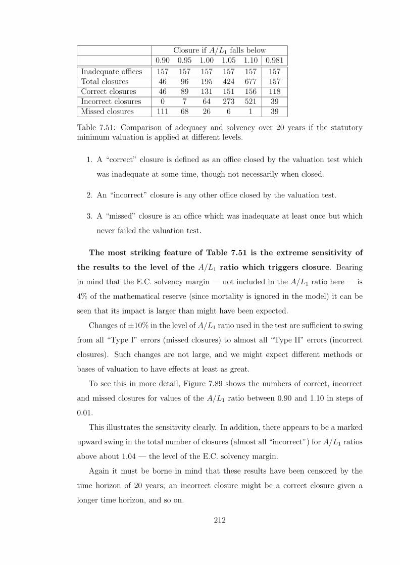
Closure if A/L1 falls below0.90 0.95 1.00 1.05 1.10 0.981
Inadequate offices 157 157 157 157 157 157Total closures 46 96 195 424 677 157Correct closures 46 89 131 151 156 118Incorrect closures 0 7 64 273 521 39Missed closures 111 68 26 6 1 39
Table 7.51: Comparison of adequacy and solvency over 20 years if the statutoryminimum valuation is applied at different levels.
1. A “correct” closure is defined as an office closed by the valuation test which
was inadequate at some time, though not necessarily when closed.
2. An “incorrect” closure is any other office closed by the valuation test.
3. A “missed” closure is an office which was inadequate at least once but which
never failed the valuation test.
The most striking feature of Table 7.51 is the extreme sensitivity of
the results to the level of the A/L1 ratio which triggers closure. Bearing
in mind that the E.C. solvency margin — not included in the A/L1 ratio here — is
4% of the mathematical reserve (since mortality is ignored in the model) it can be
seen that its impact is larger than might have been expected.
Changes of ±10% in the level of A/L1 ratio used in the test are sufficient to swing
from all “Type I” errors (missed closures) to almost all “Type II” errors (incorrect
closures). Such changes are not large, and we might expect different methods or
bases of valuation to have effects at least as great.
To see this in more detail, Figure 7.89 shows the numbers of correct, incorrect
and missed closures for values of the A/L1 ratio between 0.90 and 1.10 in steps of
0.01.
This illustrates the sensitivity clearly. In addition, there appears to be a marked
upward swing in the total number of closures (almost all “incorrect”) for A/L1 ratios
above about 1.04 — the level of the E.C. solvency margin.
Again it must be borne in mind that these results have been censored by the
time horizon of 20 years; an incorrect closure might be a correct closure given a
longer time horizon, and so on.
212

Figure 7.89: Accuracy of statutory minimum valuation basis using A/L1 ratiosbetween 0.9 and 1.1, in the baseline office.
7.3.5 A closure criterion — “equal errors”
The last column in Table 7.51 shows that applying the solvency test at the “A/L1 =
0.981” level gives equal numbers of “Type I” and “Type II” errors, and equal num-
bers of inadequacies and closures. These equalities necessarily coincide, since if we
define
CC = No. of correct closures.
IC = No. of incorrect closures.
MC = No. of missed closures.
TC = Total No. of closures.
IA = Total No. of inadequacies.
then CC +IC = TC, and CC +MC = IA, so if IC = MC it follows that TC =
IA as well. In a sense this is a neutral, if not an optimal, choice of solvency criterion,
and one which allows different valuation methods and bases to be compared. We
will use this as a basis for comparison in the later sections.
213

7.4 Aspects of the U.K. Regulations
A major theme of solvency regulation in the E.C., North America and Australia has
been the establishment of “solvency” margins in addition to mathematical reserves.
Almost the only break away from this approach has been the cash-flow tests in New
York Regulation 126 (see Section 2.7.1). In this section we consider the effect of
the two additional layers imposed under U.K. regulations; the E.C. solvency margin
and the resilience reserve.
7.4.1 The effect of the E.C. solvency margin
It is worth looking in more detail at the effect of allowing for the E.C. solvency
margin. That is, we count an office as “insolvent” if the ratio A/L1 falls below 1.04
(in the absence of mortality).
Note that the E.C. solvency margin is only taken into account for determining
solvency and not in the asset switching algorithm. This ensures that the asset mix
each year and the rate of return on the fund are the same as in the baseline office,
so the cash-flows are unchanged and hence so is the adequacy in each simulation.
Including the E.C. solvency margin in the ratio A/L2 for the purposes of asset
switching would tend to decrease the proportion in equities.
Figure 7.90 (corresponding to Figure 7.86 but to a larger scale) shows the num-
bers insolvent and inadequate in each year, and also the cumulative totals.
Clearly the incidence of insolvency is considerably greater, so that the number
of offices insolvent in any year more nearly approaches the number inadequate.
There are 353 insolvencies, of which 207 are suffered by offices which are adequate
throughout.
Figure 7.91 shows the numbers of offices at each time during the 20 years which
were inadequate, or statutorily insolvent, or both (corresponding to Figure 7.87
and to the same scale). It is now the case that an office which is insolvent at the
beginning of the period is slightly less likely to be inadequate than adequate (a
majority of “Type II” errors) while the opposite is the case in the later years.
Table 7.52 compares the times at which inadequacy and insolvency first occur,
214
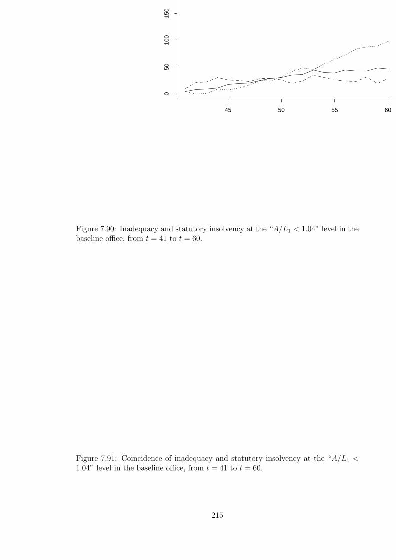
Figure 7.90: Inadequacy and statutory insolvency at the “A/L1 < 1.04” level in thebaseline office, from t = 41 to t = 60.
45 50 55 60
050
100
150
Figure 7.91: Coincidence of inadequacy and statutory insolvency at the “A/L1 <1.04” level in the baseline office, from t = 41 to t = 60.
215

Time first inadequate minustime first insolvent
Number ofoffices
5 years or more 264 years 13 years 82 years 111 year 70 year 16-1 year 64-2 years 5-3 years 1-4 years 1-5 years or less 6
Table 7.52: Comparison of times by which insolvency at the “A/L1 < 1.04” levelpreceded inadequacy in the baseline office.
in the 146 cases in which both do occur.
87 of the insolvencies occur within 1 year of inadequacy, and 103 within 2 years.
Thus the number within 1 year of inadequacy is less than before (there were 93 cases
at the “A/L1 < 1.0” level), while the number within 2 years is only 1 more than
before (there were 102 cases at the “A/L1 < 1.0” level).
Expressed as a proportion of the 146 “correct” closures, these are 59.6% within
1 year of inadequacy and 70.5% within 2 years, which may be compared with 71.0%
and 77.9% respectively at the “A/L1 < 1.0” level.
Expressed as a proportion of the total number of insolvencies, these are 24.6%
within 1 year of inadequacy and 29.2% within 2 years, compared with 47.7% and
65.0% respectively at the “A/L1 < 1.0” level.
It is worth looking at the timing of the insolvencies detected by the statutory
minimum valuation applied at different levels of the ratio A/L1, since the obser-
vations above suggest that increasing the ratio merely counts more offices to be
insolvent at some time, and not necessarily at any time close to inadequacy. Of
course, using a higher A/L1 ratio must result in some insolvent offices becoming
insolvent sooner.
Table 7.51 above showed that the accuracy of the statutory solvency valuation
is very sensitive to the A/L1 ratio which is used. Table 7.53 below shows that the
timing of closure, even of inadequate offices, is also sensitive to the A/L1 ratio.
216
Level of A/L1 ratio0.90 0.95 1.00 1.05 1.10
No. within 1 year 41 76 93 84 63% of “correct” closures 89.1% 85.4% 71.0% 55.6% 40.4%% of all insolvencies 89.1% 64.4% 47.7% 19.8% 9.3%
No. within 2 years 42 77 102 101 80% of “correct” closures 91.3% 86.5% 77.9% 66.9% 51.3%% of all insolvencies 91.3% 65.3% 52.3% 23.8% 11.8%
Table 7.53: Numbers of insolvencies within 1 or 2 years of inadequacy at variouslevels of A/L1.
Even so small a change as the addition of a 4% solvency margin alters
considerably the accuracy and timing of the statutory minimum valua-
tion. The fact that it was moderately effective in this model at the “A/L1 < 1.0”
level should not at this stage be taken as anything but coincidence, but the sen-
sitivity of the results to a small change in the reserving requirements is of some
interest.
The effect of requirements along the lines of the C-1 Risk Based Capital factors in
the U.S.A. would be even more severe. For example, the current RBC requirements
would require extra capital of at least 30% of the value of equities to be held. While
this is not unlike the U.K. resilience test as far as the assets are concerned, an
important difference is that the resilience test takes into account the effect of falls
in asset values on yields, and hence on the valuation of liabilities.
In the remainder of this section we consider the statutory minimum reserve and
resilience test together as a test of solvency.
7.4.2 The effect of the resilience reserve
It is probably unfair to regard the U.K. resilience test as a test of insolvency, in
the sense of leading to an immediate threat of closure or other serious action. It
functions as a warning of potential mismatching risks, and barring catastrophes
should allow remedial action to be taken by the office — hence its use in our asset
switching algorithm.
Should the ratio A/L2 ever fall below 1.0, however, at a time when a solvency-
driven asset allocation strategy is in use, this would indicate that the office would
217

Closure if A/L2 falls below0.90 0.95 0.99 0.9526
Inadequate offices 157 157 157 157Total closures 71 151 250 157Correct closures 71 114 139 117Incorrect closures 0 37 111 40Missed closures 86 43 18 40
Correct to 1 year 58 90 93Correct to 2 years 62 97 105
Table 7.54: Comparison of adequacy and solvency over 20 years using the ratio A/L2
as the solvency criterion.
be unable to set up the statutory minimum reserve after the change in conditions
supposed in the mismatching test, despite 100% investment in gilts, and this might
be a good enough reason for intervention to occur. Therefore we might look at the
effectiveness of a solvency test of the form “A/L2 < x”, where x < 1.0, even in
the presence of the asset switching driven by the ratio A/L2 itself. This must be a
stronger test than the statutory minimum on its own, since A/L2 ≤ A/L1.
Table 7.54 shows the numbers of correct and incorrect closures, where closure
takes place if the ratio A/L2 falls below the levels shown. Like Table 7.51, the level
at which the number of insolvencies equals the number of inadequacies is shown (in
this case, A/L2 = 0.9526). In addition, the numbers of closures which are within 1
year or 2 years of the first occurrence of inadequacy are shown.
This test is certainly not better than the statutory minimum test on its own.
Indeed at the “A/L2 < 0.99” level, there are 250 closures of which 139 are correct,
93 to within 1 year, while using the “A/L1 < 1.00” test there are 195 closures, of
which 131 are correct, 93 to within 1 year. Inspection shows that 91 of the closures
within 1 year of inadequacy are the same in both cases. Increasing the number of
incorrect closures from 64 to 111 for the sake of another 8 correct closures, but with
no significant improvement in timing, might not be thought worthwhile.
Figure 7.92 shows the numbers of closures of each type for A/L2 ratios between
0.9 and 1.0.
218
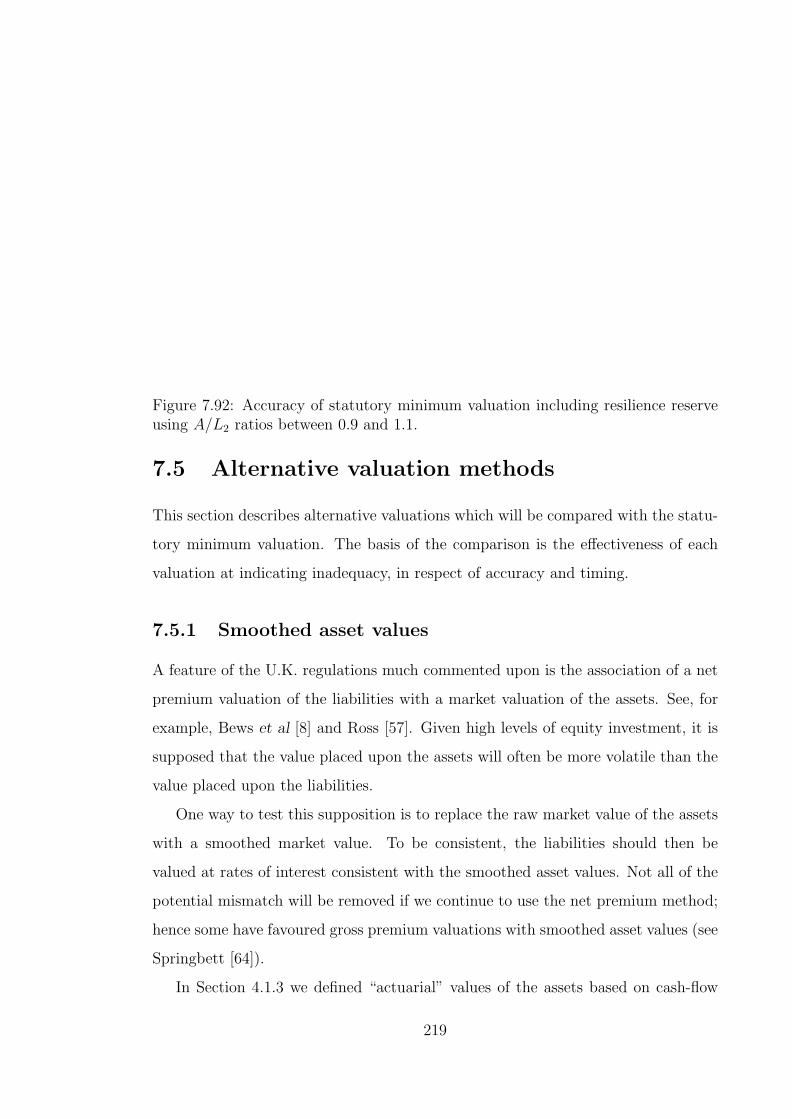
Figure 7.92: Accuracy of statutory minimum valuation including resilience reserveusing A/L2 ratios between 0.9 and 1.1.
7.5 Alternative valuation methods
This section describes alternative valuations which will be compared with the statu-
tory minimum valuation. The basis of the comparison is the effectiveness of each
valuation at indicating inadequacy, in respect of accuracy and timing.
7.5.1 Smoothed asset values
A feature of the U.K. regulations much commented upon is the association of a net
premium valuation of the liabilities with a market valuation of the assets. See, for
example, Bews et al [8] and Ross [57]. Given high levels of equity investment, it is
supposed that the value placed upon the assets will often be more volatile than the
value placed upon the liabilities.
One way to test this supposition is to replace the raw market value of the assets
with a smoothed market value. To be consistent, the liabilities should then be
valued at rates of interest consistent with the smoothed asset values. Not all of the
potential mismatch will be removed if we continue to use the net premium method;
hence some have favoured gross premium valuations with smoothed asset values (see
Springbett [64]).
In Section 4.1.3 we defined “actuarial” values of the assets based on cash-flow
219

Basis 2 - Smoothed asset valuesClosure if A/L falls below
0.90 0.95 1.00 1.05 1.10 0.979
Inadequate offices 157 157 157 157 157 157Total closures 55 117 245 402 517 157Correct closures 50 95 138 149 154 116Incorrect closures 5 22 107 253 363 41Missed closures 107 62 19 8 3 41
Correct to 1 year 42 77 90 86 79Correct to 2 years 44 82 102 103 95
Table 7.55: Comparison of adequacy and solvency over 20 years using the smoothedvaluation basis No.2 as the solvency criterion.
valuations at geometric moving average yields. Here we will take these to be our
smoothed asset values. Correspondingly we will value the liabilities at a rate of
interest which is a weighted average of the moving average yields used to value the
assets; the weights are taken to be the market values of each type of asset in the
fund.
Note that equities are valued by applying smoothed dividend yields to current
dividends. Therefore investment in equities results in a low valuation rate of interest,
just as in the statutory minimum basis. This makes comparison with the statutory
minimum basis itself easier.
We will call the statutory minimum basis “Basis 1”, and the smoothed version
described here “Basis 2”. Table 7.55 shows the accuracy of the smoothed valuation
with various levels of A/L ratio as the closure criterion.
Figure 7.93 shows the numbers of correct and incorrect closures etc. under the
smoothed valuation basis No.2.
Comparing these results with Table 7.51 and Figure 7.89 shows that the use of
smoothed yields for both asset and liability valuations reduces slightly the sensitivity
of the number of closures to the A/L ratio which is used, and in particular appears to
remove the marked increase which was apparent above A/L1 = 1.04 in Figure 7.89.
The statutory minumum basis (unsmoothed) is slightly better at the “A/L1 < 1.00”
level, closing 195 (131 correct) compared with 245 (138 correct) but both valuation
bases show such sensitivity to the A/L ratio that this is not remarkable.
Comparison with Table 7.49 suggests also that Basis No.2 using smoothed yields
220

Figure 7.93: Accuracy of valuation Basis 2 (smoothed asset values) using A/L ratiosbetween 0.9 and 1.1.
and asset values is slightly less sensitive to larger values of the A/L ratio. Although
the difference is not great, this is of some interest when the addition of a solvency
margin to a mathematical reserve is considered.
7.5.2 Static valuation bases
A feature of the U.K. statutory minimum basis is that the maximum interest rate is
calculated dynamically. To a more limited extent the same is true in the U.S.A., but
there the interest rate so calculated is applied only to new business. In other E.C.
territories the valuation basis is static, and almost always the same as the premium
basis. In this section we consider the effect of static valuation bases.
Basis 3 This is a gross premium basis, using the same interest rate of 5% and
bonus loading of 2.5% as does the premium basis. This represents, loosely,
the most common practice in E.C. territories of valuing on the premium basis,
but adapted to the method of premium calculation common in the U.K..
Basis 4 This is a net premium basis, using an interest rate of 3%. No Zillmer is
used, since there are no expenses. 3% is broadly typical of the interest rates
used in net premium valuations of taxed with-profits contracts in the U.K.. It
is rather weaker than the interest rate implied by the premiums; the annual
221
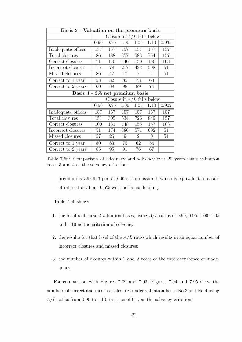
Basis 3 - Valuation on the premium basisClosure if A/L falls below
0.90 0.95 1.00 1.05 1.10 0.935
Inadequate offices 157 157 157 157 157 157Total closures 86 188 357 583 754 157Correct closures 71 110 140 150 156 103Incorrect closures 15 78 217 433 598 54Missed closures 86 47 17 7 1 54
Correct to 1 year 58 82 85 73 60Correct to 2 years 60 89 98 89 74
Basis 4 - 3% net premium basisClosure if A/L falls below
0.90 0.95 1.00 1.05 1.10 0.902
Inadequate offices 157 157 157 157 157 157Total closures 151 305 534 726 849 157Correct closures 100 131 148 155 157 103Incorrect closures 51 174 386 571 692 54Missed closures 57 26 9 2 0 54
Correct to 1 year 80 83 75 62 54Correct to 2 years 85 95 91 76 67
Table 7.56: Comparison of adequacy and solvency over 20 years using valuationbases 3 and 4 as the solvency criterion.
premium is £92.926 per £1,000 of sum assured, which is equivalent to a rate
of interest of about 0.6% with no bonus loading.
Table 7.56 shows
1. the results of these 2 valuation bases, using A/L ratios of 0.90, 0.95, 1.00, 1.05
and 1.10 as the criterion of solvency;
2. the results for that level of the A/L ratio which results in an equal number of
incorrect closures and missed closures;
3. the number of closures within 1 and 2 years of the first occurrence of inade-
quacy.
For comparison with Figures 7.89 and 7.93, Figures 7.94 and 7.95 show the
numbers of correct and incorrect closures under valuation bases No.3 and No.4 using
A/L ratios from 0.90 to 1.10, in steps of 0.1, as the solvency criterion.
222
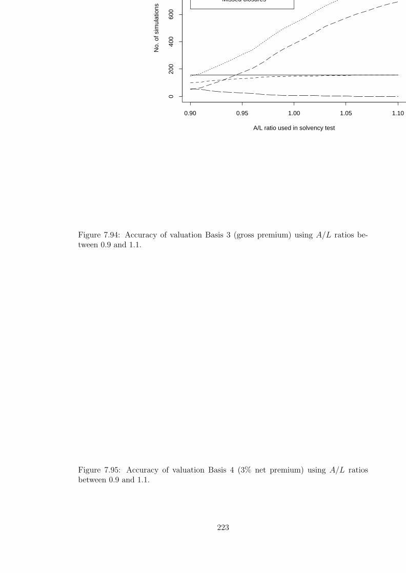
Figure 7.94: Accuracy of valuation Basis 3 (gross premium) using A/L ratios be-tween 0.9 and 1.1.
A/L ratio used in solvency test
No.
of s
imul
atio
ns
0.90 0.95 1.00 1.05 1.10
020
040
060
0
Missed closures
Figure 7.95: Accuracy of valuation Basis 4 (3% net premium) using A/L ratiosbetween 0.9 and 1.1.
223

Figure 7.96: Accuracy of valuation Basis 5 (net premium, 92.5% of gilt yield) usingA/L ratios between 0.9 and 1.1.
These figures, compared with Figures 7.89 and 7.93 show some interesting fea-
tures. However, we will introduce two further bases before drawing our conclusions.
7.5.3 Dynamic valuation methods
Basis 5 This is a net premium basis, in which the interest rate is 92.5% of the
current net redemption yield on gilts. There is no further restriction on the
yields assumed in respect of future investments. This is broadly similar to the
U.K. statutory valuation basis, with potential dividend growth allowed for but
adjusted to eliminate the risk premium relative to gilts.
Basis 6 This is a net premium basis, in which the interest rate is 63% of a 10-
year (geometric) moving average of the net redemption yield on gilts. This
approximates the “strengthened” basis proposed by the Buol committee (see
Section 2.5.2).
Table 7.57 and Figures 7.96 and 7.97 show the results.
Again these figures, compared with Figures 7.89, 7.93, 7.94 and 7.95, show some
interesting features.
1. The six bases surveyed fall into two broad categories, within each of which
224

Basis 5 - Net premium, 92.5% of gilt yieldClosure if A/L falls below
0.90 0.95 1.00 1.05 1.10 0.979
Inadequate offices 157 157 157 157 157 157Total closures 47 97 200 403 601 157Correct closures 47 89 132 151 155 117Incorrect closures 0 8 68 252 446 40Missed closures 110 68 25 6 2 40
Correct to 1 year 41 76 93 84 75Correct to 2 years 42 77 103 101 92
Basis 6 - Net premium, 63% of 10-yr average gilt yieldClosure if A/L falls below
0.90 0.95 1.00 1.05 1.10 0.935
Inadequate offices 157 157 157 157 157 157Total closures 92 190 402 618 764 157Correct closures 80 122 146 153 157 112Incorrect closures 12 68 256 465 607 45Missed closures 77 35 11 4 0 45
Correct to 1 year 63 90 84 71 59Correct to 2 years 67 100 97 87 73
Table 7.57: Comparison of adequacy and solvency over 20 years using valuationbases 5 and 6 as the solvency criterion.
A/L ratio used in solvency test
No.
of s
imul
atio
ns
0.90 0.95 1.00 1.05 1.10
020
040
060
080 Incorrect closures
Missed closures
Figure 7.97: Accuracy of valuation Basis 6 (net premium, 63% of 10-yr average giltyield) using A/L ratios between 0.9 and 1.1.
225

the results are similar. Bases No.1, No.2 and No.5 are similar; call this the
“dynamic” group; and Bases No.3, No.4 and No.6 are similar; call this the
“static” group. (Basis No.6 is not by definition static but belongs among the
static bases by virtue of its behaviour.)
2. Up to the “A/L < 1.0” level, the static bases all close about twice as many of-
fices as the dynamic bases. In this region, they behave rather like the dynamic
bases do with a higher A/L ratio.
3. Above the “A/L < 1.0” level, the numbers of closures under the dynamic bases
increases rapidly, closing the gap with the static bases. The most satisfactory
in this respect is Basis No.2, which smooths both asset and liability valuation
bases.
4. The level of A/L ratio at which exactly the same number of offices were closed
as were inadequate gives some indication of the optimum performance of a
valuation basis to an observer with no preference for “Type I” or “Type II”
errors. These “minimum” numbers of errors in every case were quite close —
between 39 and 54 — but were attained at very different levels of A/L ratio.
Under the dynamic bases, the minimum errors were attained with closure
around the “A/L < 0.97” level; under all the static bases the corresponding
A/L ratio was much lower.
What all these valuation bases have in common is the sensitivity of the
results — their ability to close the right offices in approximately good
time — to the level of the A/L ratio which is used to trigger closure.
Where they differ is in how good the “obvious” “A/L < 1.0” criterion is
compared with alternatives.
The important corollaries are (i) that the imposition of solvency margins which
effectively increase the level of the A/L ratio used as a closure criterion is a very blunt
instrument; (ii) the use of a uniform solvency margin across a variety of valuation
regimes is potentially iniquitous. Following from (ii) above is the conclusion that,
if traditional solvency valuations must be used, then the whole solvency system —
mathematical reserves, solvency margins, resilience tests etc. — should be designed
226

as a whole, in particular to avoid the duplication of margins. This the Australians
and Canadians have done; the E.C. approach is less satisfactory.
7.5.4 The A/AS ratio as a solvency criterion
As described in Chapter 1, with-profits business in the U.K. relies on the terminal
bonus system, not only to maintain solvency with high levels of equity investment,
but also for the capital with which to write new business. This is particularly true
of mutual offices.
As terminal bonuses began to form a greater part of the maturity benefit, par-
ticularly in the 1980s, some actuaries drew attention to the resulting dilution of
solvency standards, where solvency was based on a valuation of the guaranteed ben-
efits alone. It has been suggested that solvency reserves ought to allow for future
terminal bonus; see in particular Lyon [40]. Since terminal bonuses are not guar-
anteed it might not be appropriate to reserve for them in full measure, but not to
reserve at all is possibly to neglect reasonable expectations.
Where the policy asset share plays a part in the determination of terminal bonus
— upon which there is widespread though not uniform agreement in the U.K. —
then the current asset share is a natural measure of the quantum of assets needed
to meet maturity benefits. It is not sufficient on its own since it disregards the
guarantees, and it is not suitable for non-profit business, but where the terminal
bonus system is the major determinant of policyholders’ reasonable expectations
it is arguably a more logical choice than a policy value based on the guaranteed
benefits.
Consequently we will consider the A/AS ratio as a measure of “solvency” for
with-profits endowments. Table 7.58 and Figure 7.98 show the numbers of closures
for selected values of the ratio A/AS.
In two senses the A/AS ratio seems far better than any of the A/L ratios as a
solvency criterion. At the “A/AS < 1.0” level it closes only 110 offices, all of them
correctly. And at the “A/AS < 1.017” level it makes only 33 errors each of “Type
I” and “Type II”. However, relatively few of the offices closed are closed within 1 or
2 years of the first occurrence of inadequacy; the timing of the ratio A/AS seems
227
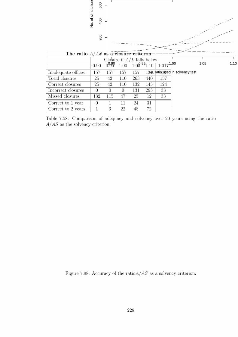
The ratio A/AS as a closure criteronClosure if A/L falls below
0.90 0.95 1.00 1.05 1.10 1.017
Inadequate offices 157 157 157 157 157 157Total closures 25 42 110 263 440 157Correct closures 25 42 110 132 145 124Incorrect closures 0 0 0 131 295 33Missed closures 132 115 47 25 12 33
Correct to 1 year 0 1 11 24 31Correct to 2 years 1 3 22 48 72
Table 7.58: Comparison of adequacy and solvency over 20 years using the ratioA/AS as the solvency criterion.
A/L ratio used in solvency test
No.
of s
imul
atio
ns
0.90 0.95 1.00 1.05 1.10
020
040
060
0
Figure 7.98: Accuracy of the ratioA/AS as a solvency criterion.
228

Time first inadequate minustime first insolvent
Number ofoffices
5 years or more 04 years 03 years 02 years 01 year 00 year 0-1 year 11-2 years 11-3 years 20-4 years 25-5 years or less 43
Table 7.59: Comparison of times by which insolvency at the “A/AS < 1.0” levelpreceded inadequacy in the baseline office.
rather poorer than that of any of the A/L ratios.
Table 7.59 shows that the timing of the A/AS ratio is, in fact, completely differ-
ent from the examples given previously of the timing of an A/L ratio. The A/AS
ratio at the “A/AS < 1.0” level does not close a single office before the occurrence
of inadequacy. Moreover, it tends to close offices long afterwards, not immediately
afterwards.
No closures occur before the first inadequacy because payment of 100% of the
asset shares as a minimum ensures that only cash-flows out of the additional estate
are possible; further, if the ratio A/AS ever falls below 1.0 a deficit is certain
following closure and run-off at any future time.
The reason closures, though all “correct”, are so late is that in most cases inad-
equacy is caused by a financial crisis during the run-off. The same financial crisis
might cause the A/AS ratio to fall below 1.0, if the office is allowed to remain open
to new business, and will trigger closure at that time. Compare Figure 7.99 with
Figure 7.88. Figure 7.99 shows the distribution of the ratio A/AS at the time of
inadequacy, and in the 10 years afterwards, for the 157 inadequate offices. Figure
7.88 showed the corresponding distribution of the ratio A/L1. It is clear that the
latter is far more responsive to inadequacy than is the A/AS ratio. A comparison
of Figures 4.9 and 4.11 confirms that the ratio A/AS is much less volatile than the
ratio A/L1, the reason being that changes in the value of assets affect numerator
229

Figure 7.99: 5th, 25th, 50th, 75th, 95th quantiles, and 10 sample paths, of the ratioA/AS following the first occurrence of inadequacy.
and denominator equally in the ratio A/AS. Therefore inadequacy related to such
changes in value might not be detected by the ratio A/AS.
7.6 Conclusions
This chapter has thrown some light on the operation of the traditional solvency
valuation. Although the model is a very simple one, some clear conclusions have
emerged.
1. There is little coincidence, from year to year, between offices which are insol-
vent and offices which are inadequate.
2. Given the same valuation basis, the number of closures (insolvencies) is sensi-
tive to the level of A/L ratio which is used as a criterion of closure.
3. Comparing different valuation bases, there are large differences between the
numbers of closures, given the same A/L ratio as a closure criterion.
4. The effect of a uniform solvency margin, even one so small as 4% of mathe-
matical reserves, can differ markedly depending on the underlying valuation
regime.
230

5. The ratio A/AS is not a satisfactory alternative to the ratio A/L as a mea-
sure of solvency, even under the circumstances of this model which reflects
somewhat retrospective management practices.
The comparison of adequacy and solvency suggests some interesting topics worth
further study.
1. The pattern of adequacy itself — constantly increasing numbers inadequate
with few recoveries from inadequacy — probably depends on the details of
the simple baseline office. In other circumstances, offices might recover from
inadequacy more frequently. We wish to investigate this in order to see how
reasonable it might be to estimate adequacy by checking run-offs at just a few
times within that time horizon (to make the computation more feasible).
2. The baseline office showed a significant but not overwhelming incidence of in-
adequacy. Do we obtain a similar relationship (or lack of it) between insolvency
and inadequacy in an office which suffers much higher levels of inadequacy?
3. The accuracy of the various solvency valuations tested above showed great
sensitivity to the level of A/L ratio which was used as a closure criterion. Is
this also the case in different circumstances?
4. The A/AS ratio appeared to be a more accurate indicator of inadequacy than
any A/L ratio, but its timing was so much worse that it is hardly to be
preferred. It is probably wrong to regard the A/L ratios examined here as
having better timing because of any predictive ability; the question really is
how many adequate offices have to be closed in order to catch enough of the
inadequate ones?
In the next chapter we investigate these questions.
231

Chapter 8
Further aspects of adequacy
8.1 Variations on the traditional valuation
In Chapter 7 we introduced adequacy and compared it with solvency, both statutory
(in the U.K.) and according to other measures. The circumstances were those of the
model described in Chapter 4; in particular the investment strategy was driven by
the ratio A/L2.
The aim of this chapter is to compare solvency and adequacy as in Chapter 7
under some different conditions, and to see if the behaviour of a particular valuation
method is consistent, or not, when applied in a range of circumstances.
The range of examples is necessarily limited, because of the time-consumimg
nature of adequacy testing. They are as follows; unless otherwise stated the mod-
ifications described are made to the office of Chapter 7, which we denote here by
“Office A”:
Office B We first look at an office with 100% in equities before closure, reduced
to 50% after closure. Although extreme, this allows direct comparison to be
made with Office A.
Office C Next we look at an office which pursues the same investment and bonus
strategies as Office A before closure, but continues to employ them without
moderation after closure. This tests the “cost” of Policyholders’ Reasonable
Expectations, insofar as they may be represented by the continuance of given
232

strategies.
Both of the above offices have this in common; that they result in a higher
number of inadequacies than does Office A. They therefore allow us to compare
adequacy and solvency under more extreme conditions.
Office D An office with 70% in equities before closure, 35% after closure. These
levels are fixed; the office does not employ the solvency-driven asset switching
algorithm of Office A. This level of equity investment is typical of practice in
the U.K..
Office E An office with 100% of its funds in gilts and a terminal bonus target of
nil (i.e. aiming to pay all its benefits in guaranteed form). This approximates
to the practice in some territories outside the U.K., notably Germany.
These last two offices result in lower numbers of inadequacies than in Office
A. They therefore allow us to compare adequacy and solvency under less extreme
conditions. Finally, we consider two offices with some of the features considered in
earlier chapters.
Office F An office with the “combined smoothing” algorithm of Chapter 6. This
results in the additional estate being credited with increments to the Bonus
Smoothing Account, as well as being debited under the operation of the guar-
antees.
Office G An office in which the resilience test is modified along the lines of the
Government Actuary’s Memorandum of 30 September 1993, by testing a rise
of 1.5% in the dividend yield and a proportionate change of ±20% in the gilt
yield. The U.K. resilience test continues to develop, with the evident aim of
making it suited to a wider range of circumstances; this is worth testing.
In Chapter 7, we considered the effect of 6 valuation bases in some detail, in-
cluding the use of different A/L ratios as a solvency criterion. In this chapter, we
will show less detail to aid comparison. For each office we will show:
233

Figure 8.100: Inadequacy and statutory insolvency in Office A, from t = 41 tot = 60.
1. The numbers inadequate and statutorily insolvent each year, and the corre-
sponding cumulative totals.
2. The effect of varying the A/L ratio used as the closure criterion under the
statutory minimum solvency test only.
3. The effect of using the valuation bases No.2 – No.6 defined in Section 7.5, and
the ratio A/AS, each at the same (A/L < 1.0) level.
4. The A/L ratio at which each of these solvency tests achieves equal numbers
of “Type I” and “Type II” errors.
In what follows, figures comparable to Figure 7.86 will be shown, so that the
build-up of inadequacy and insolvency can be compared with that in Office A.
However, in some cases the numbers of inadequacies or insolvencies are too great for
the scale used in Figure 7.86. For convenience, therefore, Figure 8.100 reproduces
Figure 7.86 to the same scale as will be used in this chapter.
234

Figure 8.101: Inadequacy and statutory insolvency in Office B (fixed 100% in equi-ties), from t = 41 to t = 60.
8.2 Offices with higher levels of inadequacy
8.2.1 Office B: 100% in equities
In Office B the investment strategy is fixed, at 100% in equities before closure and
50% in equities after closure. It is thus the same as Office A except for the removal
of the dynamic investment strategy. Figure 8.101 shows the numbers of simulations
resulting in statutory insolvency and inadequacy each year, and the cumulative
totals of the same.
The total number of inadequacies is 316. As in Office A, recovery from inade-
quacy is infrequent; at time t = 70 the number then inadequate is 294. The total
number of statutory insolvencies is 645, so while the number of inadequacies has
doubled, the number of insolvencies has trebled.
Figure 8.102 shows the numbers of correct and incorrect closures etc. under
the statutory minimum valuation basis. It shows graphically the effect of a harsh
valuation; even at the “A/L < 0.90” level the test is far too strong, and increasing
the A/L ratio simply catches more adequate offices. It would be wrong to say that
a weak test is wanted here, since 316 inadequacies out of 1,000 is hardly impressive,
but this test seems to deploy its strength in the wrong places.
235
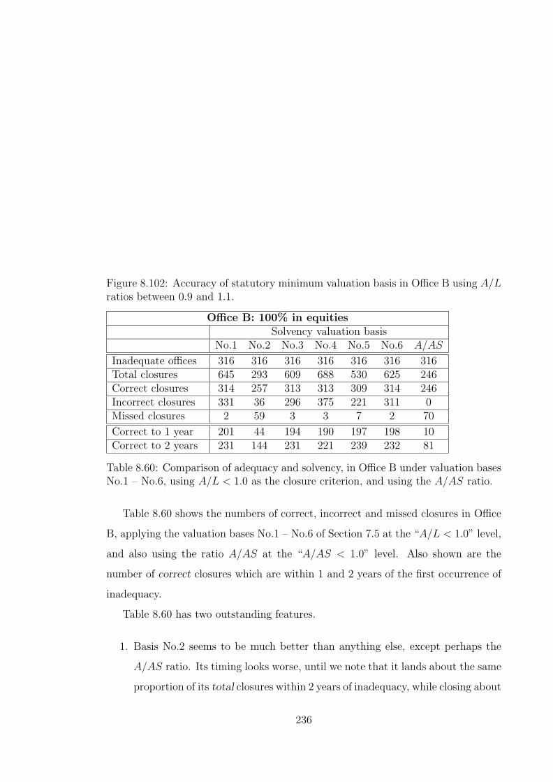
Figure 8.102: Accuracy of statutory minimum valuation basis in Office B using A/Lratios between 0.9 and 1.1.
Office B: 100% in equitiesSolvency valuation basis
No.1 No.2 No.3 No.4 No.5 No.6 A/AS
Inadequate offices 316 316 316 316 316 316 316Total closures 645 293 609 688 530 625 246Correct closures 314 257 313 313 309 314 246Incorrect closures 331 36 296 375 221 311 0Missed closures 2 59 3 3 7 2 70
Correct to 1 year 201 44 194 190 197 198 10Correct to 2 years 231 144 231 221 239 232 81
Table 8.60: Comparison of adequacy and solvency, in Office B under valuation basesNo.1 – No.6, using A/L < 1.0 as the closure criterion, and using the A/AS ratio.
Table 8.60 shows the numbers of correct, incorrect and missed closures in Office
B, applying the valuation bases No.1 – No.6 of Section 7.5 at the “A/L < 1.0” level,
and also using the ratio A/AS at the “A/AS < 1.0” level. Also shown are the
number of correct closures which are within 1 and 2 years of the first occurrence of
inadequacy.
Table 8.60 has two outstanding features.
1. Basis No.2 seems to be much better than anything else, except perhaps the
A/AS ratio. Its timing looks worse, until we note that it lands about the same
proportion of its total closures within 2 years of inadequacy, while closing about
236

Figure 8.103: Accuracy of valuation Basis No.2 (smoothed asset and liability valu-ation bases) in Office B using A/L ratios between 0.9 and 1.1.
200 fewer adequate offices.
2. Using the A/AS ratio as a solvency criterion also looks to be more effective,
except that as in Chapter 7 its timing is very poor.
Basis No.2 looks so much better, it is worth looking at how sensitive it is to
changes in the A/L ratio used as the closure criterion. This is shown in Figure
8.103.
Considering the extreme investment strategy, the shortness of the policy term
and the contrast with Figure 8.102, Basis No.2 seems to be remarkably insensitive
to the level of the A/L ratio which is used. This was remarked upon also in Section
7.5.1, but it is much more striking here.
Table 8.61 shows the “optimum” performance of each solvency test, in the sense
of closing exactly the same number of offices as are inadequate (equivalently, making
equal numbers of “Type I” and “Type II” errors).
The most obvious feature in Table 8.61, this time including Basis No.2, is how
similar the “best” efforts of each basis are. Given 1,000 offices, 316 inadequacies,
and upon being invited to choose 316 offices to close, Bases No.1 – No.6 get between
267 and 278 correct. In addition, the “optimum” A/L ratios are all similar apart
from Basis No.2.
237

Office B: 100% in equitiesSolvency valuation basis
No.1 No.2 No.3 No.4 No.5 No.6 A/AS
“Optimum” A/L ratio 0.830 1.022 0.831 0.801 0.876 0.833 1.054
Inadequate offices 316 316 316 316 316 316 316Total closures 316 316 316 316 316 316 316Correct closures 278 267 272 273 277 274 281Incorrect closures 38 49 44 43 39 42 35Missed closures 38 49 44 43 39 42 35
Table 8.61: Comparison of adequacy and solvency in Office B, at the A/L ratiosyielding “equal errors” under under valuation bases No.1 – No.6, and using theA/AS ratio.
This table, along with the tables in Section 7.5, suggest that all valuation bases
will do a similar job provided we can find the appropriate level of A/L ratio to use
as a solvency criterion. Unfortunately, that level is not the intuitively appealing
“A/L < 1.0”. Even less is it “A/L < 1.04”.
8.2.2 Office C: same strategies after closure
In Office A three strategies are amended after closure; the upper limit on equity
investment is cut to 50%, the terminal bonus target is increased to 50%, and the
allowable drop in reversionary bonus rates is doubled to 40%. In Office C these
changes are not made, so no concession is made to the changed circumstances. Such
a test represents a rigid interpretation of policyholders’ reasonable expectations.
Figure 8.104 shows the numbers of simulations resulting in statutory insolvency
and inadequacy each year, and the cumulative totals of the same. (Note again that
this is not to the same scale as Figure 7.86.)
The number of inadequacies has more than doubled; in total there are 368. Of
these, only 215 are inadequate at time t = 70, so there is a much higher incidence
of recovery from inadequacy. However, the numbers of statutory insolvencies are
exactly the same as before (because the strategies are identical before closure).
This changes the relative patterns of inadequacy and insolvency. There is now a
considerable number of inadequacies at outset (69), and where before the total of
insolvencies always outran the total of inadequacies, now it is the other way round.
238

Figure 8.104: Inadequacy and statutory insolvency in Office C (same strategies afterclosure), from t = 41 to t = 60.
So much so, that the cumulative number of insolvencies never exceeds the current
number of inadequacies.
This is an interesting observation; the actions of the managers after clo-
sure have a significant effect on adequacy, not just in the long term but
on immediate closure too. Statutory minimum solvency makes no such
distinctions.
Figure 8.105 shows the numbers of correct and incorrect closures etc. under the
statutory minimum valuation basis.
This is quite different to the corresponding figures in respect of Offices A and B.
The point emerging here is that the same valuation basis, applied to offices using
different strategies, can give quite different results. Note that (i) Offices A, B and C
are identical at the starting point, time t = 40, and (ii) Offices B and C differ only
in the degree of caution which might be employed during a run-off.
Table 8.62 shows the effect of the valuation bases No.1 – No.6 of Section 7.5 at
the “A/L < 1.0” level.
The numbers of closures in this table are the same as under Office A in Chapter
7. Again the harshness of the static valuation bases No.2 (premium basis) and
No.3 (3% net premium) is apparent. In addition, such small proportions of the
closures are within 2 years of inadequacy that none of these bases can be described
239

Figure 8.105: Accuracy of statutory minimum valuation basis in Office C using A/Lratios between 0.9 and 1.1.
Office C: Same strategies before and after closureSolvency valuation basis
No.1 No.2 No.3 No.4 No.5 No.6 A/AS
Inadequate offices 368 368 368 368 368 368 368Total closures 195 245 357 534 200 402 110Correct closures 168 196 238 303 171 269 110Incorrect closures 27 49 119 231 29 133 0Missed closures 200 172 130 65 197 99 258
Correct to 1 year 16 18 24 31 16 24 1Correct to 2 years 20 25 29 44 20 31 1
Table 8.62: Comparison of adequacy and solvency, in Office C under valuation basesNo.1 – No.6, using A/L < 1.0 as the closure criterion, and using the A/AS ratio.
240

Office C: Same strategies before and after closureSolvency valuation basis
No.1 No.2 No.3 No.4 No.5 No.6 A/AS
“Optimum” A/L ratio 1.043 1.041 1.002 0.965 1.045 0.996 1.077
Inadequate offices 368 368 368 368 368 368 368Total closures 368 368 368 368 368 368 368Correct closures 267 267 242 240 268 254 245Incorrect closures 101 101 126 127 100 113 123Missed closures 101 101 126 127 100 113 123
Table 8.63: Comparison of adequacy and solvency in Office C, at the A/L ratiosyielding “equal errors” under under valuation bases No.1 – No.6, and using theA/AS ratio.
as particularly accurate; but here again, the A/AS ratio is by far the poorest.
Table 8.63 shows the “optimum” (equal errors) performance of each solvency
test.
8.3 Offices with lower levels of inadequacy
8.3.1 Office D: 70% in equities
In Chapter 5, fixed asset allocation strategies were compared with solvency-driven
strategies, over a 30-year time horizon, with the result that 100% investment in eq-
uities with solvency-driven asset switching gave rise to the same number of statutory
insolvencies as 60% – 70% investment in equities without the asset switching.
In Office D, the proportions in equities are fixed as 70% before closure and 35%
after closure. Figure 8.106 shows the numbers and cumulative totals of inadequacies
and statutory insolvencies.
The total number of inadequacies is almost halved compared with Office A (85
instead of 157). However, the number of statutory insolvencies has increased (232
instead of 195). This confirms the outcome of Office B; that solvency is more
sensitive than adequacy to the difference between a fixed and a solvency-driven
asset allocation strategy. It also agrees with the conclusion of Ross & McWhirter
[58].
Figure 8.107 and Table 8.64 show the effects of various valuation bases.
241

Figure 8.106: Inadequacy and statutory insolvency in Office D (70% in equities),from t = 41 to t = 60.
A/L ratio used in solvency test
No.
of s
imul
atio
ns
0.90 0.95 1.00 1.05 1.10
020
040
060
0
Missed closures
Figure 8.107: Accuracy of statutory minimum valuation basis in Office D using A/Lratios between 0.9 and 1.1.
242

Office D: 70% in equitiesSolvency valuation basis
No.1 No.2 No.3 No.4 No.5 No.6 A/AS
Inadequate offices 85 85 85 85 85 85 85Total closures 232 67 241 338 185 256 46Correct closures 79 55 78 81 76 79 46Incorrect closures 153 12 163 257 109 177 0Missed closures 6 30 7 4 9 6 39
Correct to 1 year 60 11 59 54 58 60 1Correct to 2 years 65 35 64 60 68 64 8
Table 8.64: Comparison of adequacy and solvency, in Office D under valuation basesNo.1 – No.6, using A/L < 1.0 as the closure criterion, and using the A/AS ratio.
Office D: 70% in equitiesSolvency valuation basis
No.1 No.2 No.3 No.4 No.5 No.6 A/AS
“Optimum” A/L ratio 0.889 1.022 0.884 0.850 0.910 0.869 1.048
Inadequate offices 85 85 85 85 85 85 85Total closures 85 85 85 85 85 85 85Correct closures 57 61 53 53 59 57 66Incorrect closures 28 24 32 32 26 28 19Missed closures 28 24 32 32 26 28 19
Table 8.65: Comparison of adequacy and solvency in Office D, at the A/L ratiosyielding “equal errors” under under valuation bases No.1 – No.6, and using theA/AS ratio.
Again, Basis No.2 stands out, especially compared with No.1, the statutory
minimum basis. Table 8.65 shows the “optimum” performance of each solvency
test.
The pattern of previous examples is repeated; the range of A/L ratios at which
equal numbers of errors are attained is quite wide, and the numbers of errors are
very similar for under all the tests except the A/AS ratio.
8.3.2 Office E: A traditional “fixed-interest” office
Office E represents a “traditional” fixed-interest, reversionary bonus office. The
starting point at time t = 40 is the same as in Office A, but then (i) the assets are
switched to 100% in gilts, and (b) the terminal bonus target is changed from 25%
to 0%. This does not mean that the terminal bonus paid is always nil — if the asset
243

Office E: “Traditional” fixed interestSolvency valuation basis
No.1 No.2 No.3 No.4 No.5 No.6 A/AS
“Optimum” A/L ratio 0.889 1.022 0.884 0.850 0.910 0.869 1.048
Inadequate offices 0 0 0 0 0 0 0Total closures 0 0 29 78 0 0 0Correct closures 0 0 0 0 0 0 0Incorrect closures 0 0 29 78 0 0 0Missed closures 0 0 0 0 0 0 0
Table 8.66: Comparison of adequacy and solvency in Office E, at the A/L ratiosyielding “equal errors” under under valuation bases No.1 – No.6, and using theA/AS ratio.
shares at maturity exceed the guaranteed benefits then a terminal bonus is paid as
usual — but that the office does not use terminal bonus in a strategic way. Table
8.66 shows the effect of the valuation bases No.1 – No.6.
There are now no inadequacies. (The question of “how close” the office might
be to inadequacy will be dealt with in Section 8.6.) More interesting, there are
no insolvencies either under any of the dynamic valuation bases. In fact, there
are no insolvencies under the statutory minimum basis (No.1) even if the solvency
criterion is increased to “A/L < 1.10”. There are, however, insolvencies under the
static valuation bases. This confirms their relative harshness.
8.4 Other changes
8.4.1 Office F: Introducing smoothing
In Chapter 6 several methods of smoothing maturity benefits were introduced. Here
we examine the effect of one of them on adequacy and solvency. Office F is the same
as Office A except that the “combined” smoothing defined in Section 6.2.3 is used; in
this, the assets underlying the maturing policy’s asset shares are smoothed first, and
then limits are aplied to the year-on-year changes in maturity values. Figure 8.108
shows the numbers and cumulative totals of inadequacies and statutory insolvencies.
The total number of inadequacies has increased from 157 to 233, and the total
number of statutory insolvencies has also increased from 195 to 248.
244

Figure 8.108: Inadequacy and statutory insolvency in Office F (“combined smooth-ing” from Chapter 7), from t = 41 to t = 60.
Office F: “Combined” smoothingSolvency valuation basis
No.1 No.2 No.3 No.4 No.5 No.6 A/AS
Inadequate offices 233 233 233 233 233 233 233Total closures 248 292 442 597 252 469 211Correct closures 185 197 212 223 186 220 173Incorrect closures 63 95 230 374 66 249 38Missed closures 48 36 21 10 47 13 60
Correct to 1 year 115 121 125 119 116 131 8Correct to 2 years 143 146 146 139 145 153 40
Table 8.67: Comparison of adequacy and solvency, in Office F under valuation basesNo.1 – No.6, using A/L < 1.0 as the closure criterion, and using the A/AS ratio.
Figure 8.109 and Table 8.67 show the results under the various valuation bases.
The main difference between this and previous tables is the A/AS ratio; it is
much more comparable with the dynamic valuation bases (which in turn are much
less harsh than the static bases). This is a consequence of the flows to and from
the additional estate resulting from smoothing; previously, when all the cash-flows
were out of the additional estate, the A/AS ratio falling below 1.0 made a deficit
inevitable in any subsequent run-off, so no “incorrect closures” were possible with
the “A/AS < 1.0” criterion. Its timing is still markedly poorer than the prospective
solvency tests, however.
245

Figure 8.109: Accuracy of statutory minimum valuation basis in Office F using A/Lratios between 0.9 and 1.1.
Office F: “Combined” smoothingSolvency valuation basis
No.1 No.2 No.3 No.4 No.5 No.6 A/AS
“Optimum” A/L ratio 0.993 0.981 0.943 0.909 0.991 0.941 1.006
Inadequate offices 233 233 233 233 233 233 233Total closures 233 233 233 233 233 233 233Correct closures 180 181 165 166 178 180 178Incorrect closures 53 52 68 67 55 53 55Missed closures 53 52 68 67 55 53 55
Table 8.68: Comparison of adequacy and solvency in Office F, at the A/L ratiosyielding “equal errors” under under valuation bases No.1 – No.6, and using theA/AS ratio.
Table 8.68 shows the “optimum” performance of each solvency test. The A/AS
ratio now joins the other solvency tests, which again have similar numbers of “equal
errors”.
8.4.2 Office G : An amended resilience test
In 1993 the resilience test used by the G.A.D. in the U.K. was amended as described
in Section 2.6. The purpose of the change was to make the test more appropriate
in a wider range of circumstances, the fixed parameters of the original (1985) test
having caused problems when yields had been at extremely high or low levels.
246

Figure 8.110: Inadequacy and statutory insolvency in Office G (amended resiliencetest), from t = 41 to t = 60.
In Office G the parameters of the resilience test are changed from their original
values of a 25% fall in equity prices, and a ±3% change in gross fixed-interest yields,
to a rise of 1.5% in the dividend yield and a proportionate change of ±20% in the
fixed-interest yield. This is therefore a similar, though not identical, test to that
now used by the G.A.D..
Note that the asset allocation is driven by the same criterion as in Office A —
100% in equities, but switch into gilts if necessary to keep the ratio A/L2 above 1.0
— but that the denominator L2 of this ratio now allows for the amended resilience
test. Therefore when comparing this with Office A, we will be interested in whether
or not the amended resilience test (i) improves statutory solvency (i.e. switches
into gilts at more appropriate times and/or in more appropriate quantities); (ii)
improves adequacy; (iii) improves the accuracy of the statutory minimum valuation.
Figure 8.110 shows the numbers and cumulative totals of inadequacies and statutory
insolvencies.
The total number of inadequacies is hardly changed from Office A; up from 157
to 165. Of these, 127 are in common (i.e. in 127 scenarios inadequacy occurs in both
Office A and Office G). The total number of insolvencies is also nearly the same;
down from 195 to 191. Of these, 165 are in common.
Figure 8.111 and Table 8.69 show the effects of the various valuation bases.
247

Figure 8.111: Accuracy of statutory minimum valuation basis in Office G using A/Lratios between 0.9 and 1.1.
Office G: 1993 resilience testSolvency valuation basis
No.1 No.2 No.3 No.4 No.5 No.6 A/AS
Inadequate offices 165 165 165 165 165 165 165Total closures 191 227 382 554 197 431 111Correct closures 126 136 140 155 126 153 111Incorrect closures 65 91 242 399 71 278 0Missed closures 39 29 25 10 39 12 54
Correct to 1 year 94 98 94 84 93 95 7Correct to 2 years 101 106 103 96 100 104 20
Table 8.69: Comparison of adequacy and solvency, in Office G under valuation basesNo.1 – No.6, using A/L < 1.0 as the closure criterion, and using the A/AS ratio.
248

Office G: 1993 resilience testSolvency valuation basis
No.1 No.2 No.3 No.4 No.5 No.6 A/AS
“Optimum” A/L ratio 0.992 0.979 0.941 0.908 0.991 0.941 1.021
Inadequate offices 165 165 165 165 165 165 165Total closures 165 165 165 165 165 165 165Correct closures 118 122 101 102 118 111 124Incorrect closures 47 43 64 63 47 55 41Missed closures 47 43 64 63 47 55 41
Table 8.70: Comparison of adequacy and solvency in Office G, at the A/L ratiosyielding “equal errors” under under valuation bases No.1 – No.6, and using theA/AS ratio.
Table 8.69, compared with the corresponding tables in Chapter 7, shows that
the amended resilience test makes very little difference to this model.
Table 8.70 shows the “optimum” performance of each solvency test.
Again, the amended resilience test makes little difference.
8.5 Discussion
The results from Offices B – G above, simple though the models are, suggest that
the conclusions of Chapter 7 are not entirely peculiar to the circumstances of Office
A which was used there. We can say that:
1. The same valuation basis may behave quite differently in the cir-
cumstances of different offices.
2. One office can suffer more inadequacies than another, but fewer
insolvencies.
3. Different management of the same office in future can radically alter both
adequacy and solvency, not necessarily in the same direction.
4. There is no consistent pattern to the strength or weakness of a given valuation
basis in different circumstances, except perhaps the harshness of the static
bases compared with the dynamic bases.
249

5. The addition of a uniform solvency margin to a traditional reserve
not only gives inconsistent results if different valuation bases are
used, but also between one office and another.
6. In the different circumstances of these offices, there is great similarity (within
each office) between the numbers of “equal errors” attained by the prospective
valuations at the “optimum” level of the A/L ratio.
7. The A/AS ratio has not been shown to be any better a measure of adequacy
than any of the dynamic prospective bases.
8. The recent amendments to the U.K. resilience test have only a small effect on
this model.
These conclusions do not give any encouragement to the employment of solvency
margins on top of traditional valuation reserves, or at least not uniform solvency
margins. The systems of RBC margins in the U.S.A., and MCCSR margins in
Canada, are more office-specific than the E.C. margins; moreover they are used in
conjunction with more uniform reserving bases. All the evidence, however, from the
work described in Chapter 3, the moves towards cash-flow testing in North America,
and the simple models described here, points away from prescribed margins and
towards cash-flow analysis.
This does not solve the regulator’s problems; on the contrary it creates a problem.
If traditional valuations are not a reliable measure of strength — though it might
be fairer to actuaries past to say that they have been rendered unreliable by the
evolution of modern practices — what to use instead? There must, for pragmatic
reasons, be some test of strength.
Following on from the above, we suggest such a test which is based on adequacy.
As a result, it is completely office-specific, and has nothing to do with prescribed
bases or margins (unless the regulator specifies the asset model and its parameters).
The suggested measure is the estimated additional assets needed to avoid inad-
equacy. The projections of run-offs, as well as revealing which scenarios give rise
to deficits (inadequacies) also reveal how bad is the inadequacy. The amount of
any deficit after the run-off can be discounted back to the starting point, using the
250

earned rates of return in the particular scenario; the result is a measure of the addi-
tional assets which would have extinguished the deficit. (Under dynamic investment
strategies, this might only be approximate.) Given a large enough number of sce-
narios, suitable quantiles of these discounted deficits indicate the additional assets
needed to avoid inadequacy with given probability.
Essentially this measure is the same as was used by the FASWP (Chapter 3),
but applied to an ongoing life office instead of to a single tranche of business.
In the remainder of this chapter, we investigate (i) the additional assets needed
to avoid inadequacy, in the examples of Offices A – G above; and (ii) whether or not,
in these simple models, adequacy can reasonably be measured using fewer run-offs
than we have used.
8.6 The adequacy margin
In this section we define an adequacy margin which measures the magnitude of an
office’s inadequacy.
The definition follows the Faculty of Actuaries Solvency Working Party’s ap-
proach to the calculation of adequacy margins in [37]. Given the projected cash-
flows assuming that the office is closed at time t, the assets remaining after the last
policy has matured can be discounted back to the starting point of the projection.
Let the result be X. If X is positive, there was a surplus after the run-off; if X
is negative there was a deficit. Since we think naturally of holding extra assets to
meet a deficit, we define the adequacy margin for closure at time t to be
−X
Asset shares at the starting point of the projection
We will usually express adequacy margins as a percentage of the asset shares at
outset.
The adequacy margin is — sometimes exactly and sometimes approximately —
the answer to the question “what extra assets (as a proportion of the asset shares)
should be held now in order to close the office in t years’ time and run off the liabilities
with zero surplus?” A positive adequacy margin means that extra assets are needed;
a negative adequacy margin means that the assets are more than sufficient.
251

In the case of the offices with solvency-driven asset allocation strategies, the
adequacy margin does not give exactly the assets needed to eliminate the run-off
surplus. This is because the asset allocation depends on the ratio A/L2, and if assets
equal in value to the adequacy margin were actually added to the office’s assets this
would, in some cases, alter the asset allocation and hence the rates of return. If the
asset allocation strategy is independent of the office’s total assets, then the adequacy
margin does give exactly the assets needed to eliminate the run-off surplus.
In terms of adequacy, a positive adequacy margin for closure at time t indicates
inadequacy at time t, and a negative margin indicates adequacy.
The discounting of the run-off surplus or deficit is perhaps most naturally carried
out at the rates of return earned on the fund, although there are other possibilities.
For example, solvency margins identified as such might be invested in fixed-interest
assets. Or, adequacy margins which formed part of an office’s free assets might be
invested in equities. In this section, the rate of return on the fund will be used.
First we investigate the adequacy margins arising in the baseline office, Office A,
before comparing these with the corresponding margins in Offices B – G.
8.6.1 Adequacy margins in Office A
Figure 8.112 shows the 5th, 25th, 50th, 75th, and 95th quantiles, and 10 sample
paths, of the adequacy margin for closure at times t = 41 to t = 60, as a percentage
of the asset shares at outset.
Some features of this figure require explanation.
1. Since the office pays 100% of the asset share on maturity, or the guaranteed
benefits if these are greater, the adequacy margin is −20% in those simulations
in which the guarantees are never called upon. In such cases, the benefits are
met entirely out of the policies’ own resources (the policy asset shares) and the
additional estate of 20% of the asset shares at time t = 40 falls into surplus
after the run-off. This explains why the 5th percentile is constant at −20%.
2. , For the same reason, the 25th and 50th quantiles are −20% of asset shares
at outset. The 75th and 95th quantiles are higher than −20% at outset,
252

Figure 8.112: 5th, 25th, 50th, 75th, 95th quantiles, and 10 sample paths, of theadequacy margin (as % of asset shares at outset).
indicating that the proportion of simulations in which that the guarantees
exceed the asset shares of maturing policies at least once during the run-off,
following closure at time t = 41, lies between 50% and 75%.
3. The adequacy margins tend to be non-decreasing, again because at least 100%
of asset shares are paid to maturing policies. Decreases are still possible,
however, because the run-off surpluses are not necessarily discounted at the
same rates of return (Closing the office at different times might alter the ratio
A/L2 after closure and hence the asset mix.) But many of the sample paths
are level for considerable periods; these indicate simulations in which the office
was able to maintain 50% in equities during the whole run-off, following closure
during these periods.
Given a time horizon, the size of the adequacy margin needed to survive closure
at any time during that time horizon can be calculated for each simulation. Let
AM i,t be the adequacy margin for closure at time t in the ith simulation. Then a
margin
AM i = maxt
AM i,t
is needed to survive closure at any time t during the time horizon in the ith
253
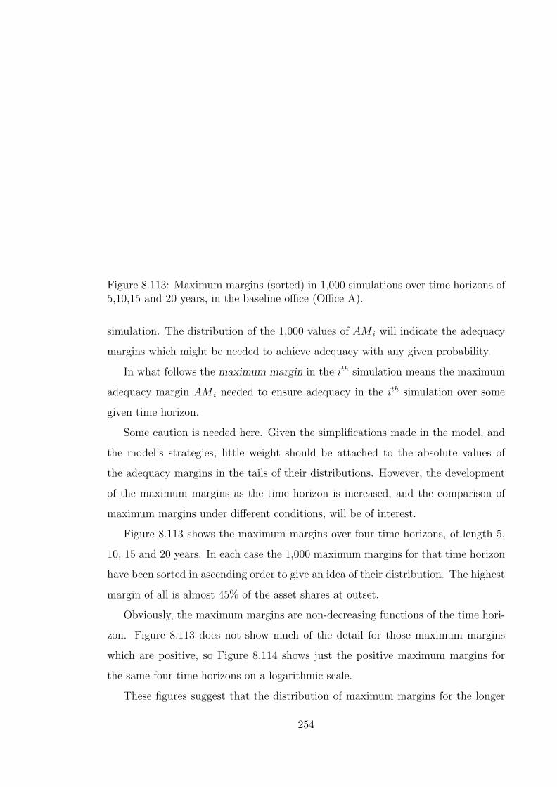
Figure 8.113: Maximum margins (sorted) in 1,000 simulations over time horizons of5,10,15 and 20 years, in the baseline office (Office A).
simulation. The distribution of the 1,000 values of AM i will indicate the adequacy
margins which might be needed to achieve adequacy with any given probability.
In what follows the maximum margin in the ith simulation means the maximum
adequacy margin AM i needed to ensure adequacy in the ith simulation over some
given time horizon.
Some caution is needed here. Given the simplifications made in the model, and
the model’s strategies, little weight should be attached to the absolute values of
the adequacy margins in the tails of their distributions. However, the development
of the maximum margins as the time horizon is increased, and the comparison of
maximum margins under different conditions, will be of interest.
Figure 8.113 shows the maximum margins over four time horizons, of length 5,
10, 15 and 20 years. In each case the 1,000 maximum margins for that time horizon
have been sorted in ascending order to give an idea of their distribution. The highest
margin of all is almost 45% of the asset shares at outset.
Obviously, the maximum margins are non-decreasing functions of the time hori-
zon. Figure 8.113 does not show much of the detail for those maximum margins
which are positive, so Figure 8.114 shows just the positive maximum margins for
the same four time horizons on a logarithmic scale.
These figures suggest that the distribution of maximum margins for the longer
254

Figure 8.114: Maximum margins (sorted) in 1,000 simulations over time horizons of5,10,15 and 20 years, in the baseline office (Office A) on a log scale.
Moments and quantiles of maximum marginsQuantiles
Time horizon Mean s.d. 90th 95th 99th41 to 45 −16.24 6.17 −7.38 −3.01 5.0641 to 50 −12.99 7.96 −1.38 1.57 13.3141 to 55 −10.44 8.73 0.43 4.28 17.6541 to 60 −8.35 8.91 1.63 5.69 19.48
Table 8.71: Moments and quantiles of maximum margins (expressed as % of assetshares at t = 40) in the baseline office (Office A) over different time horizons.
time horizons is approximately linear below zero and approximately exponential
above zero
Figure 8.114 also shows the 95% and 99% points of the maximum margins.
These, along with the 90% points and the first two moments, are shown in Table
8.71.
The 90%, 95% and 99% points suggest what additional resources would be needed
at outset, as a percentage of asset shares at outset, to ensure adequacy with these
given probabilities. However, as mentioned above the absolute values ought not to
be given too much weight.
It is worth pointing out, however, that the ratio A/L1 at outset is 1.38, which
appears to indicate that the office could reduce its assets by 33.3% of the asset
255
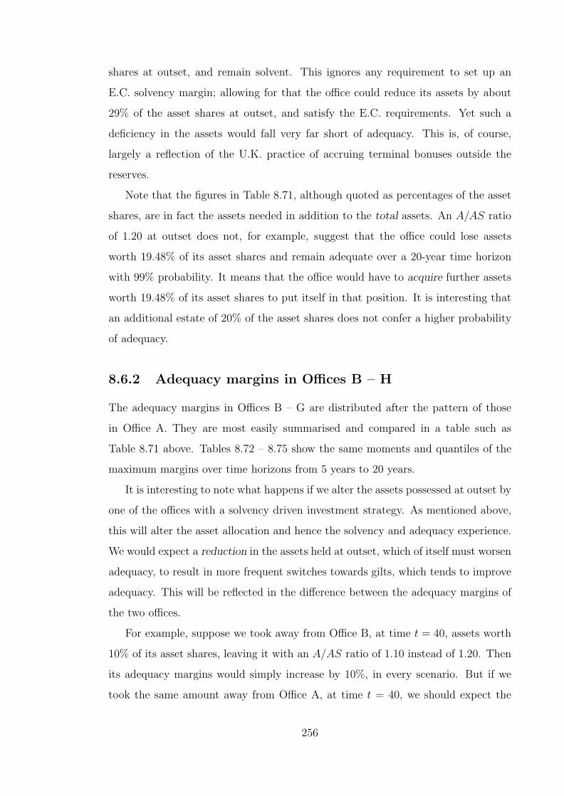
shares at outset, and remain solvent. This ignores any requirement to set up an
E.C. solvency margin; allowing for that the office could reduce its assets by about
29% of the asset shares at outset, and satisfy the E.C. requirements. Yet such a
deficiency in the assets would fall very far short of adequacy. This is, of course,
largely a reflection of the U.K. practice of accruing terminal bonuses outside the
reserves.
Note that the figures in Table 8.71, although quoted as percentages of the asset
shares, are in fact the assets needed in addition to the total assets. An A/AS ratio
of 1.20 at outset does not, for example, suggest that the office could lose assets
worth 19.48% of its asset shares and remain adequate over a 20-year time horizon
with 99% probability. It means that the office would have to acquire further assets
worth 19.48% of its asset shares to put itself in that position. It is interesting that
an additional estate of 20% of the asset shares does not confer a higher probability
of adequacy.
8.6.2 Adequacy margins in Offices B – H
The adequacy margins in Offices B – G are distributed after the pattern of those
in Office A. They are most easily summarised and compared in a table such as
Table 8.71 above. Tables 8.72 – 8.75 show the same moments and quantiles of the
maximum margins over time horizons from 5 years to 20 years.
It is interesting to note what happens if we alter the assets possessed at outset by
one of the offices with a solvency driven investment strategy. As mentioned above,
this will alter the asset allocation and hence the solvency and adequacy experience.
We would expect a reduction in the assets held at outset, which of itself must worsen
adequacy, to result in more frequent switches towards gilts, which tends to improve
adequacy. This will be reflected in the difference between the adequacy margins of
the two offices.
For example, suppose we took away from Office B, at time t = 40, assets worth
10% of its asset shares, leaving it with an A/AS ratio of 1.10 instead of 1.20. Then
its adequacy margins would simply increase by 10%, in every scenario. But if we
took the same amount away from Office A, at time t = 40, we should expect the
256

Time horizon 5 years (t = 41 – t = 45)Moments and quantiles of maximum margins
QuantilesOffice Mean s.d. 90th 95th 99th
A −16.241 6.167 −7.380 −3.010 5.056B −15.128 9.551 −5.067 3.210 23.316C −10.566 9.429 1.649 5.704 18.837D −18.720 3.456 −16.005 −12.379 −3.600E −19.744 0.192 −19.530 −19.477 −19.343F −15.655 8.367 −4.953 −0.279 12.173G −16.210 6.198 −7.236 −2.694 6.180
H −7.718 4.101 −3.072 −0.058 9.057
Table 8.72: Moments and quantiles of maximum margins (expressed as % of assetshares at t = 40) in Offices A – H over a 5-year time horizon.
Time horizon 10 years (t = 41 – t = 50)Moments and quantiles of maximum margins
QuantilesOffice Mean s.d. 90th 95th 99th
A −12.995 7.957 −1.376 1.570 13.312B −10.158 14.863 6.185 21.439 55.697C −7.588 9.961 4.170 8.494 22.709D −16.892 6.086 −10.239 −3.744 9.029E −18.769 0.600 −18.215 −17.999 −17.074F −12.002 10.001 1.769 6.642 18.921G −13.133 7.671 −1.488 1.418 8.925
H −5.881 5.073 0.416 3.178 12.525
Table 8.73: Moments and quantiles of maximum margins (expressed as % of assetshares at t = 40) in Offices A – H over a 10-year time horizon.
adequacy margins to increase by less than 10%, because of the compensating shifts
towards gilts. We therefore define Office H as follows:
Office H Office H is identical to Office A, except that we have reduced its additional
estate at time t = 40 to 10% of the asset shares instead of 20%.
These tables show some very interesting points.
1. These margins are additions to the total assets, though expressed as percent-
ages of the asset shares. Therefore the existence of a 20% additional estate
(10% for Office H) does not mean that margins up to +20% are acceptable.
Only negative margins are acceptable.
257
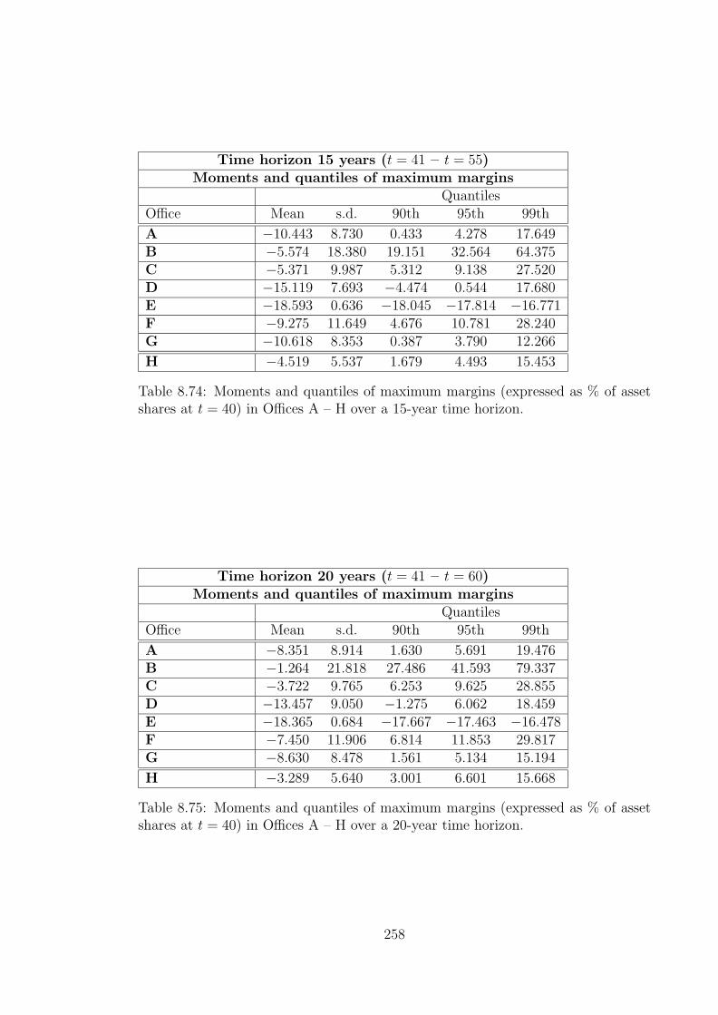
Time horizon 15 years (t = 41 – t = 55)Moments and quantiles of maximum margins
QuantilesOffice Mean s.d. 90th 95th 99th
A −10.443 8.730 0.433 4.278 17.649B −5.574 18.380 19.151 32.564 64.375C −5.371 9.987 5.312 9.138 27.520D −15.119 7.693 −4.474 0.544 17.680E −18.593 0.636 −18.045 −17.814 −16.771F −9.275 11.649 4.676 10.781 28.240G −10.618 8.353 0.387 3.790 12.266
H −4.519 5.537 1.679 4.493 15.453
Table 8.74: Moments and quantiles of maximum margins (expressed as % of assetshares at t = 40) in Offices A – H over a 15-year time horizon.
Time horizon 20 years (t = 41 – t = 60)Moments and quantiles of maximum margins
QuantilesOffice Mean s.d. 90th 95th 99th
A −8.351 8.914 1.630 5.691 19.476B −1.264 21.818 27.486 41.593 79.337C −3.722 9.765 6.253 9.625 28.855D −13.457 9.050 −1.275 6.062 18.459E −18.365 0.684 −17.667 −17.463 −16.478F −7.450 11.906 6.814 11.853 29.817G −8.630 8.478 1.561 5.134 15.194
H −3.289 5.640 3.001 6.601 15.668
Table 8.75: Moments and quantiles of maximum margins (expressed as % of assetshares at t = 40) in Offices A – H over a 20-year time horizon.
258

2. The margins in Office E — the “traditional” office — are all quite close to
−17%, and do not vary much with the time horizon. This shows that the cost
of meeting the guarantees is easily contained by the 20% additional estate,
despite paying a minimum of 100% of the asset shares on maturity.
3. All the offices except Office E require additional assets at the 95% level over
the longer time horizons. Even Office D does not escape.
4. Offices A, B, C, F and G are identical at time t = 40 — the point
at which adequacy is being measured. They differ only in the strategies
which are employed after time t = 40. Offices B and C differ only in the
strategies which will be employed during a run-off. Offices A and F differ only
in the smoothing of benefits. Yet the maximum margins are different, each
reflecting the future strategies. Traditional valuations, based entirely on an
office’s current state, are completely blind to this source of variation. Dynamic
Solvency Testing in Canada, whatever its faults in falling back on the MCCSR
test, has at least this strength: the actuary has to have regard to the likely
actions of management, given the circumstances of each scenario tested (hence
the “Dynamic”).
5. We saw, in Chapter 7, and again in this chapter, that a uniform solvency
margin could have different effects depending on the circumstances of the office,
and on the valuation method in use. The maximum margins shown here are
estimates of additional margins needed to avoid ruin with given probability —
“true” solvency margins in one sense — and the range of different answers
is another point against uniform solvency margins. Note that every
office including Office H has the same total of asset shares at outset, so these
maximum margins are comparable.
6. Office H, despite having lost assets worth 10% of its asset shares compared
with Office A, does not have maximum margins 10% higher (as a percentage
of asset shares at t = 40).
• The mean maximum margins are about 8.5% higher over a 5-year time
horizon, but only about 5% higher over a 20-year time horizon.
259

• The standard deviations of the maximum margins are lower over all time
horizons.
• The upper quantiles of the maximum margin in Office H never exceed
those in Office A by more than 5%, and over longer time horizons the
95th and 99th quantiles are even sl lower than those in Office A.
This example is worth looking at from the opposite point of view: suppose we
started with Office H, and carried out projections of adequacy margins (as we
have done). Suppose our (or the government’s) criterion was “no more than
5% chance of ruin over a 10-year time horizon” (this does not seem excessive).
Then Table 8.73 shows that additional assets equal to 3.178% of asset shares
are required. Now suppose that, with proper actuarial prudence, we said
“3.178% good — 10% better!”. We have now transformed Office H into Office
A, and note that the investment strategy is identical in both offices. But
the improvement in the additional estate simply allows management to invest
more in equities, more often, with the result that if we re-do the calculation
of adequacy margins, Table 8.73 tells us that we need another 1.57% of asset
shares on top of the extra-prudent 10% we had already added.
In this example, an asset allocation strategy driven by solvency had this un-
fortunate side-effect. But clearly any strategy which regards “free” assets,
however defined, as available for investment in riskier assets will do the same.
Such approaches to “free” assets are extremely common in the U.K..
8.7 Testing adequacy at less frequent intervals
In Office A and some others, very few offices ever recovered from adequacy. In such
cases, it might be reasonable to test for adequacy over any given time horizon by
testing adequacy at one time only — at the end of the time horizon. For example, in
Office A there were 157 cases of inadequacy during 20 years, and of these 143 were
inadequate at time t = 60. Therefore, had we tested adequacy only at time t = 60,
instead of at all times t = 41, 42, . . . , 60, we would only have missed 14 cases, or
about 10% of the total. This might be considered a reasonable price to pay, given
260

Office C Office FTime t Number Cum. tot. Number Cum. tot.
t = 45 100 155 41 47t = 50 141 232 94 117t = 55 183 310 139 183t = 60 215 368 155 233
Table 8.76: Numbers and cumulative totals inadequate at 5-yearly intervals in Of-fices C and F.
the enormous reduction in computing time.
Ross & McWhirter [58] effectively do this, using a time horizon of 40 years. They
found that only 1 simulation (out of 49) resulted in a deficit after closure at the end
of 40 years, or in our terms only one inadequacy out of 49 at time 40 years after
the start. If their office, like Office A, was such that few inadequate offices recover,
then their result is a fair indication of the ability of that office to transact business
over the next 40 years. If, however, their office is such that temporary spells of
inadequacy are more common, then the test they applied is too weak. In particular,
it is then inconsistent to compare statutory insolvency occurring in any of the 40
years with inadequacy only at the end of 40 years.
Two of the offices above display reasonable rates of recovery from adequacy; Of-
fice C (with the same strategies before and after closure) and office F (with maturity
benefit smoothing). Table 8.76 shows the numbers inadequate, and the cumulative
totals of inadequacies, at 5-yearly intervals in these offices.
It is obvious that if we were to test the adequacy of either of these offices only
at time t = 60, we would form a much more favourable view of their adequacy than
would be justified by the facts. Indeed, if we compared office F with Office A on
this basis, (155 inadequacies instead of 143) we would conclude that smoothing had
a much milder effect than the cumulative totals suggest (233 inadequacies instead
of 157).
Note that Ross & McWhirters’ model included two features — benefit smoothing
and a charge on the asset shares — which make it likely that it has some of the
properties of Office F.
However, testing adequacy in every future year is laborious, so it is still worth
knowing if sampling inadequacy in just a few future years gives reasonable results.
261
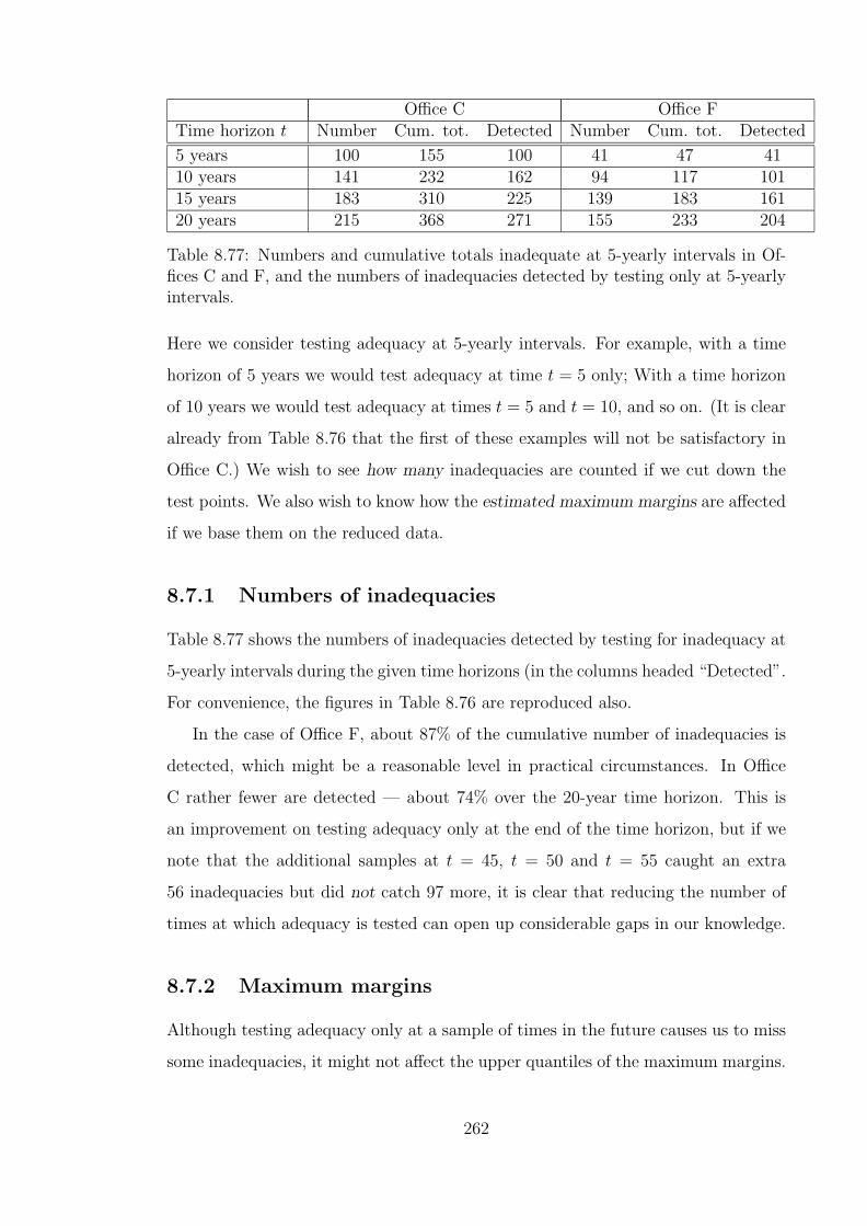
Office C Office FTime horizon t Number Cum. tot. Detected Number Cum. tot. Detected
5 years 100 155 100 41 47 4110 years 141 232 162 94 117 10115 years 183 310 225 139 183 16120 years 215 368 271 155 233 204
Table 8.77: Numbers and cumulative totals inadequate at 5-yearly intervals in Of-fices C and F, and the numbers of inadequacies detected by testing only at 5-yearlyintervals.
Here we consider testing adequacy at 5-yearly intervals. For example, with a time
horizon of 5 years we would test adequacy at time t = 5 only; With a time horizon
of 10 years we would test adequacy at times t = 5 and t = 10, and so on. (It is clear
already from Table 8.76 that the first of these examples will not be satisfactory in
Office C.) We wish to see how many inadequacies are counted if we cut down the
test points. We also wish to know how the estimated maximum margins are affected
if we base them on the reduced data.
8.7.1 Numbers of inadequacies
Table 8.77 shows the numbers of inadequacies detected by testing for inadequacy at
5-yearly intervals during the given time horizons (in the columns headed “Detected”.
For convenience, the figures in Table 8.76 are reproduced also.
In the case of Office F, about 87% of the cumulative number of inadequacies is
detected, which might be a reasonable level in practical circumstances. In Office
C rather fewer are detected — about 74% over the 20-year time horizon. This is
an improvement on testing adequacy only at the end of the time horizon, but if we
note that the additional samples at t = 45, t = 50 and t = 55 caught an extra
56 inadequacies but did not catch 97 more, it is clear that reducing the number of
times at which adequacy is tested can open up considerable gaps in our knowledge.
8.7.2 Maximum margins
Although testing adequacy only at a sample of times in the future causes us to miss
some inadequacies, it might not affect the upper quantiles of the maximum margins.
262

Time horizon 20 years (t = 41 – t = 60)Moments and quantiles of maximum margins
QuantilesTime horizon Mean s.d. 90th 95th 99th
Office C
5 years −11.526 8.625 −0.043 3.793 17.27010 years −8.789 9.293 2.437 6.207 18.86815 years −6.627 9.373 3.643 7.098 22.19220 years −4.997 9.154 4.765 8.099 23.607
Office F
5 years −18.458 9.458 −5.786 −0.841 12.17310 years −14.157 10.823 0.023 6.294 18.92115 years −11.3 12.328 4.346 9.969 25.72120 years −9.308 12.557 6.298 11.061 26.516
Table 8.78: Moments and quantiles of maximum margins (expressed as % of assetshares at t = 40) in Offices C and F, with adequacy tested at 5-yearly intervals only.
Intuitively, those simulations which produce the worst results are more likely to be
inadequate for longer, and hence have a higher chance of being detected. They are
also more likely to be represented in the upper quantiles of the distribution of the
maximum margin.
We will widen the definition of a maximum margin from that above,
AM i = maxt
AM i,t
so that the maximum is taken over the set of times t at which adequacy is tested,
which now need not be every year during the time horizon. Table 8.78 shows the
moments and quantiles of the resulting distributions of maximum margins for time
horizons of 5, 10, 15 and 20 years, with adequacy tested at 5-yearly intervals.
Comparing this with Tables 8.72 – 8.75, we see that the upper quantiles of the
maximum margins are reduced by comparatively little; in practical terms the figures
in Table 8.78 might be quite reasonable lower bounds to the more accurately — and
laboriously — computed figures.
263
8.8 Conclusions
1. The same valuation basis, applied to different offices, varies in its effectiveness
compared with the run-off cash-flows.
2. The strategies used by the office’s managers have a very great effect on ade-
quacy, including strategies after closure which do not affect the assessment of
solvency.
3. The effect of a uniform solvency margin on the accuracy of a traditional val-
uation also depends very much on the individual circumstances.
4. Adequacy margins based on the distributions of projected run-off deficits are
also very dependent on future strategies, again including strategies after clo-
sure.
5. Estimating maximum margins by projecting closure and run-off at a smaller
set of future times underestimates the numbers of future inadequacies but (in
this model) yields quite good lower bounds for maximum margins.
264

Chapter 9
Summary
In this chapter we summarise the conclusions of the preceding chapters, but first
we will state our main conclusion. The wide range of strategies available to
life office managers, even allowing for constraints such as PRE, make
prescriptive or mechanical measurement of financial strength unreliable.
Traditional tools such as solvency valuations and uniform solvency mar-
gins give inconsistent results in different circumstances. It is necessary
to allow for the features of individual offices and their managements in
assessing financial strength.
9.1 The development of solvency assessment
Until the development of computers, the measurement of solvency relied upon
present values based upon particularly simple models of future economic conditions.
The assets in which funds were invested, however, were such that the simple models
gave workable tools for measuring solvency and surplus. The outcomes in respect of
Office E in Chapter 8 suggest that fixed-interest investment combined with suitable
bonus rules would would allow a simple office to be managed tolerably well with
traditional solvency valuations.
The volatility of inflation, yields and equity prices since the 1950s has made the
traditional “constant interest rate” model look unrealistic. Moreover, with-profits
funds have invested heavily in equities and properties during that time. Therefore
265
the model underlying solvency valuations is, qualitatively, unlike the experience of
the corresponding assets.
Concerns about the effectiveness of solvency valuations have been pursued in
three main directions (see Chapter 2).
1. Mandatory or minimum valuation bases have been prescribed in territories
where there is no premium tariff and no practice of valuing on the premium
basis — principally in the U.K., the U.S.A. and Canada.
2. Additional margins have been prescribed to strengthen these mathematical re-
serves — the E.C. solvency margins, RBC requirements in the U.S.A., MCCSR
in Canada and the U.K. resilience test.
3. Tests which are less prescriptive and more specific to the features of individual
companies have been developed, notably Dynamic Solvency Testing in Canada
but also in the U.S.A. and Australia.
Some of the RBC and MCCSR margins have been based on tail probabilities in
stochastic studies, but in the main the details of these rules have been determined
in ad hoc ways or by sensitivity analyses within the traditional model. A particu-
lar criticism of the E.C. solvency margins is their application to a broad range of
valuation regimes and methods. Even Canadian DST is based on projections of the
results of traditional solvency valuations.
An alternative approach to solvency is to find stochastic replacements for the
traditional valuation models, and to examine the distribution of projected outcomes,
in particular estimated ruin probabilities. Solvency reserves are then determined as
the funds needed to limit ruin probabilities to some small value (see Chapter 3).
9.2 Life office modelling in the U.K.
Models of U.K. with-profits life offices must allow for the considerable degree of
discretion given to managers to control asset allocation, bonus and smoothing strat-
egy, and perhaps other factors too (see Chapters 3 and 4). The strategies which are
266
chosen have a considerable effect on the outcomes, including solvency. Among the
questions which arise are those considered in this thesis:
1. How much of the fund should be invested in equities?
2. What should be the balance between reversionary and terminal bonuses?
3. How should investment returns be smoothed?
4. How should financial strength be measured?
A simple model office, writing 10-year with-profit endowment business, was set
up. In order to focus on asset allocation and bonus strategies, (i) mortality, lapses
and expenses were excluded and (ii) the office was taken to be in a state of stable
and sustainable growth as a starting point. The model was the basis for a series
of simulation studies, using the Wilkie Reduced Standard model of inflation, fixed-
interest yields and equity returns.
9.3 Equity investment and statutory insolvency
In Chapter 4 the circumstances leading to statutory insolvency in the model were
investigated, particularly in the light of the suggestion made in a previous study
that low inflation has an adverse effect on solvency. The main conclusions were:
1. There was some indication that the distribution of the rate of inflation was
low in the years preceding insolvency, but the sample paths did not show the
same feature. Thus low inflation — or its consequences — could not provide
a clear mechanism of failure.
2. Statutory insolvency was strongly associated with catastrophic falls in share
prices. This association was a property of the sample paths.
3. Falls in share prices were influenced largely by the white noise components of
the dividend yield model and dividend index models. Inflation was a lesser
influence.
267

9.4 Asset allocation strategies
Previous studies using the Wilkie asset model have compared equity and gilt (fixed-
interest) investment and concluded that the former achieves much higher mean re-
turns but with a much higher variance of returns; therefore equity investment is
“riskier”. In Chapter 5 a range of asset allocation strategies were studied, particu-
larly their effects on (i) maturity values and (ii) statutory solvency.
The conclusion above was confirmed in terms of nominal maturity values, but
examination of real maturity values suggested that the relative safety of gilts may
be overstated; the variance of real maturity values under gilt investment, relative to
that under equity investment, was much less than the variance of nominal maturity
values. On the other hand, investment in equities led to much higher numbers of
statutory insolvencies.
The asset allocation strategy was modified along the lines suggested by Ross
[57] to switch from equities to gilts when necessary in order to maintain statutory
solvency; this did cut the numbers of insolvencies considerably, but only by allowing
asset switches of up to 100% of the fund in a single year. Restricting the proportion
of the fund switched in a single year to a lower level (25%) removed much of the
advantage of the solvency-driven asset switching.
A range of dynamic asset allocation strategies was studied, including declining
EBR, cyclical and contracyclical strategies. On the basis of nominal maturity val-
ues, the contracyclical strategies performed better than their cyclical counterparts,
giving higher mean maturity values with less variability, and slightly better than
the corresponding fixed investment strategy. On the basis of real maturity values,
cyclical strategies displayed the lower variability.
Changes to the reversionary bonus strategy made relatively little difference, pos-
sibly due in part to the short term of the business.
9.5 Maturity value smoothing
In Chapter 6 the effect of maturity value smoothing was investigated. Smoothing
is often cited as one of the “hallmarks” of with-profits business, particularly in
268

conjunction with equity investment. It is usually assumed that the long-term costs of
smoothing will balance out. However, in this model the cost of smoothing (measured
by the ratio BSA/AS) was not necessarily stable over time; the accumulated historic
costs of smoothing were considerable in certain cases.
1. Two methods of smoothing cited by respondents to an industry survey were
studied. Smoothing of maturity values appeared to be more effective than
smoothing of asset values, and it absorbed a larger part of the cost of the
guarantees, but at the expense of stability of the accumulated cost of smooth-
ing.
2. The relative cost of smoothing was sensitive to the rate of new business growth;
high growth contained the cost but there appeared to be considerable danger
in smoothing while new business was declining.
3. Applying a simple form of feedback to control the level of the ratio BSA/AS
was not successful, because the need to meet the guarantees prevented the
feedback from being applied in adverse circumstances. In fact, any method
which limited the volatility of the ratio BSA/AS appeared to be vulnerable
to the incidence of the guarantees.
4. The cost of smoothing depends on the stability of the asset model, particularly
if the assets are revalued. The sensitivity of equity values to dividend yields
is a particular risk.
9.6 Inadequacy versus insolvency
In Chapters 7 and 8 the accuracy and timing of traditional solvency valuations were
measured by comparing the valuation results with subsequent run-offs in each of
1,000 scenarios. The term “adequacy” was used to indicate a surplus after a run-off.
1. There was little coincidence, from year to year, between offices which were
statutorily insolvent and offices which were inadequate. Over a long time,
however, the statutory valuation succeeded in detecting a fairly high propor-
tion of inadequate offices.
269

2. The number of insolvencies was very sensitive to the level of A/L ratio which
was used as a criterion of closure. Therefore the imposition of a uniform
solvency margin, even one as small as 4% of mathematical reserves, can have
a considerable and to a large extent arbitrary effect.
3. Different valuation methods and bases resulted in large differences between
the numbers of insolvencies. In particular, fixed (static) bases seemed to be
markedly harsher than dynamic bases including the U.K. statutory minimum
basis. It follows that the effect of a uniform solvency margin, depends very
strongly on the underlying valuation regime.
4. The ratio A/AS was not a satisfactory alternative to the ratio A/L as a
measure of solvency.
As well as the effect of different valuation bases on the same office, the effect of the
same valuation bases on different offices was considered. The broad conclusion was
that both (i) the outcomes and (ii) the effectiveness of a traditional valuation varied
markedly from office to office. The strategies used by the office’s managers had a
very great effect on adequacy, including strategies after closure which had no effect
on the assessment of solvency. A uniform solvency margin in these circumstances
does not lead to any specific improvement in the solvency valuation.
The simulated distribution of the discounted surpluses and deficits after run-offs
allows adequacy margins to be estimated, namely additional assets sufficient to avoid
inadequacy with some given probability. These margins are also very dependent on
the strategies used by the managers; in particular high equity investment requires
high margins. There was no link between the level of adequacy margins and any
traditional valuation reserve.
In some cases offices were found to recover from adequacy with reasonably high
frequency, making it necessary to test run-offs from every possible time of closure
in order to measure adequacy within any given time horizon. Some limited trials
suggested that reasonable lower bounds of adequacy margins for given time horizons
might nevertheless be found by projecting run-offs following closure at a limited set
of future times.
270

9.7 Further questions
The questions which we have explored here, in an empirical way, raise a host of
further questions, many concerned with relaxing the strong simplifying assumptions
made here. We can only indicate some possible lines for further research.
1. What is the effect of a mixture of business of different terms on the cost of
smoothing and the comparison between solvency and adequacy?
2. It is unlikely that the premium rate would remain fixed in the face of the very
low rates of return which occur in some scenarios. What is the effect of a
premium-setting strategy?
3. The traditional with-profits endowment is being replaced by the unitised with-
profits contract in some market sectors. Many aspects of the management of
unitised with-profits business remain to be decided; for example there is no
agreement on valuation methods. What is the effect of this new bonus system
on adequacy?
4. How might option pricing or hedging strategies be incorporated into asset
allocation and bonus strategies? Do such approaches offer a stronger basis for
the measurement and control of surplus than a traditional valuation?
5. What effect does the pattern of new business, and surrenders, in the past and
in the future, have on the working out of the in-force?
6. How do different starting conditions — for example, an additional estate —
affect the outcomes?
7. What is the effect of changing the asset model? Alternatives to Wilkie’s AR(1)
model of inflation have been suggested, for example ARCH models: are sol-
vency and adequacy sensitive to such assumptions?
271

References
[1] Allport K.F. et al (1991). Proposals for a Standard for the Determination
of Statutory Reserves. Presented to the Institute of Actuaries of Australia
Convention, Hobart, 1991.
[2] Ammeter H. (1966). The Problem of Solvency in Life Assurance. J. Inst. Ac-
tuaries 92 p.193.
[3] Ammeter H. (1967). The Natural and Mechanical Methods of Assessing Sol-
vency Reserves in Life Assurance. J. Inst. Actuaries 93 p.79.
[4] Baker A. C., Graham N. S. (1977). Some Thoughts on Solvency of Life Assur-
ance Companies. Trans. Faculty of Actuaries 35 p.474.
[5] Bayley G. V., Perks W. (1953). A Consistent System of Investment and Bonus
Distribution for a Life Office. J. Inst. Actuaries 79 p.14.
[6] Benjamin S. et al. (1980). Report of the Maturity Guarantees Working Party.
J. Inst. Actuaries 107 p.103.
[7] Benz N. (1959). Some Notes on Bonus Distributions by Life Offices. J. Inst.
Actuaries 86 p.1.
[8] Bews R.P., Seymour P. A. C., Shaw A. N. D., Wales F. R. (1976). Proposals
for the Statutory Basis of Valuation of the Liabilities of Long-term Insurance
Business. Trans. Faculty of Actuaries 34 p.367.
[9] Brender A. (1984). Required Surplus for the Insurance Risk for Certain Lines
of Group Insurance. Trans. Soc. Actuaries XXXVI p.9.
272

[10] Brender A. (1991). The Evolution of Solvency Standards for Life Assurance
Companies in Canada. Presented to the Institute of Actuaries of Australia
Convention, Hobart, 1991.
[11] Brindley B., Dumbreck N., Thomson C., Thompson S. (1990). Policyholders’
Reasonable Expectations. Report of a Joint Faculty and Institute Working
Party. Presented to a seminar on Current Issues in Life Assurance, Birming-
ham, 10 July 1990.
[12] Buol et al. (1971). Financial Guarantees Required from Life Assurance Con-
cerns. Organisation for Economic Co-operation and Development, Paris, 1971.
[13] Campagne (1957). Minimum Standards of Solvency for Insurance Firms. Or-
ganisation for European Economic Co-operation.
[14] Campagne (1961). Minimum Standards of Solvency for Insurance Firms. Re-
port of the ad hoc Working Party on Minimum Standards of Solvency. Organ-
isation for European Economic Co-operation.
[15] Cody D. D. (1988). Probabilistic Concepts in Measurement of Asset Adequacy.
Trans. Soc. Actuaries XL p.149.
[16] Debenham D. W. et al. (1989). Asset Share Techniques and the Control of Ter-
minal Bonuses. Proceedings of the 3rd U.K. Actuarial Convention, Harrogate,
17–19 September 1989, p.144.
[17] Dunsford G. A. et al (1991). A Standard for the Determination of Policy
Reserves. Presented to the Institute of Actuaries of Australia Convention,
Hobart, 1991.
[18] Eastwood A. M. et al of the Faculty of Actuaries Bonus and Valuation Re-
search Group. With Profits Maturity Payouts, Asset Shares and Smoothing.
To appear in Trans. Faculty of Actuaries 44.
[19] Elgin W. F. (1963). Letter to the Editor. Trans. Faculty of Actuaries 28 p.227.
[20] Elliott S.F. (1988). Some Aspects of the Statutory Valuation. J. Inst. Actuaries
Students’ Soc. 31 p.127.
273

[21] Fine A. E. M. (1972). A discussion of techniques for forecasting the devel-
opment of a life assurance company. Transactions of the 19th International
Congress of Actuaries, Oslo 1972, 2 p.87.
[22] Forfar D. O. et al. of the Faculty of Actuaries Bonus and Valuation Research
Group (1989). Bonus Rates, Valuation and Solvency During the Transition
between Higher and Lower Investment Returns. Trans. Faculty of Actuaries
40 p.490.
[23] Forrest J. et al (1991). Current Topics. Presented to the Faculty of Actuaries
Students’ Society, Edinburgh, 4 March 1991.
[24] Freeman M., Vincent B. (1991). Capital Adequacy in Life Insurance — a
Survey of Overseas Developments. Presented to the Institute of Actuaries of
Australia Convention, Hobart, 1991.
[25] Frees E. W. (1990). Stochastic Life Contingencies with Solvency Considera-
tions. Trans. Soc. Actuaries XLII p.91.
[26] Geoghegen T. J. et al. (1992). Report on the Wilkie Stochastic Investment
Model. J. Inst. Actuaries 119 p.173.
[27] Gulland C. M. (1948). Letter to the Editor. Trans. Faculty of Actuaries 18
p.355.
[28] Gulland C. M. (1956). Letter to the Editor. Trans. Faculty of Actuaries 25
p.91.
[29] Hardy M. R. (1993). Stochastic Simulation in Life Assurance Solvency. J. Inst.
Actuaries 120 p.131.
[30] Haynes A. T., Kirton R. J. (1953). The Financial Structure of a Life Office.
Trans. Faculty of Actuaries 21 p.141.
[31] Hylands J. F. et al of the Joint Actuarial Working Party. Joint Actuarial
Working Party No.3 — Risk Based Capital, Interim Report. Presented to
the Life Convention of the Faculty of Actuaries and Institute of Actuaries,
Blackpool, November 1993.
274

[32] Insurance Companies Act 1982 (1982). H.M.S.O..
[33] The Insurance Companies Regulations 1981 (1981). H.M.S.O.
[34] The Insurance Companies Regulations 1994 (1994). H.M.S.O.
[35] Kennedy S. P. L. et al (1977). Bonus Distribution with High Equity Backing.
J. Inst. Actuaries 103 p.11.
[36] Kitts A. (1990) Comments on a Model of Retail Price Inflation. J. Inst. Actu-
aries 117 p.407.
[37] Limb A. P. et al. of the Faculty of Actuaries Solvency Working Party (1986).
The Solvency of Life Assurance Companies. Trans. Faculty of Actuaries 39
p.251.
[38] Lang J., Scott W. A. (1993). Profit Reporting in a Mutual Office. To appear
in Trans. Faculty of Actuaries.
[39] Ljeskovac M. et.al. of the Faculty of Actuaries Mortality Research Group
(1991). A Model Office Investigation of the Potential Impact of AIDS on Non-
linked Life Assurance Business. Trans. Faculty of Actuaries 42 p.187.
[40] Lyon C. S. S. (1988). The Financial Management of a With Profit Long Term
Fund — Some Questions of Disclosure. J. Inst. Actuaries 115 p.111.
[41] Macauley F. R. (1938) Some Theoretical Problems Suggested by the Move-
ments of Interest Rates, Bond Yileds and Stock Prices in the United States
since 1856. National Bureau of Economic Research, New York.
[42] Macdonald A. S. (1991) On Investment Strategies Using the Wilkie Model.
Transactions of the 2nd AFIR International Colloquium Brighton 1991 3
p.413.
[43] Macdonald A. S. (1993) What is the Value of a Valuation?. Transactions of
the 3rd AFIR International Colloquium Rome 1993 2 p.725.
[44] Macdonald A. S. (1994) A Note on Life Office Models. Trans. Faculty of Ac-
tuaries 44 p.63.
275
[45] Macdonald A. S. (1994) Appraising Life Office Valuations. Transactions of the
4th AFIR International Colloquium Orlando 1994 3 p.1163.
[46] Murray A. C. (1937). The Investment Policy of Life Assurance Offices. Trans.
Faculty of Actuaries 16 p.247.
[47] Needleman P. (1992). Resilience Testing Within the Current Regulatory
Framework. Seminar on “Current Issues in Life Assurance”, Staple Inn, 12
November 1992.
[48] Norberg R. (1991). Reserves in Life and Pensions Insurance. Scand. Actuarial
J. 1991 p.3.
[49] Norberg R., Møller C. M. (1993). Theile’s Differential Equation by Stochastic
Interest of Diffusion Type. University of Copenhagen Working Paper No.117.
[50] Oppe T. H. M. (1971). The Implications for British Insurance, Particularly
Long-Term Business, of Joining the European Common Market. Trans. Fac-
ulty of Actuaries 33 p.20.
[51] Paul D. R. L. et al. of the Faculty of Actuaries Bonus and Valuation Research
Group (1993). Restructuring Mutuals — Principles and Practice. Trans. Fac-
ulty of Actuaries 43 p.167.
[52] Pentikainen T. et al of the Finnish Insurance Modelling Group (1994). On the
Asset Models as a part of All-Company Insurance Analysis. Transactions of
the 4th AFIR International Colloquium Orlando 1994 3 p.1471.
[53] Pukkila T., Ranne A., Sarvamaa S. (1994) On Stochastic Modeling of Inflation.
Transactions of the 4th AFIR International Colloquium Orlando 1994 2 p.589.
[54] Purchase D. E. et al. (1990). Reflections on Resilience — Some Considerations
of Mismatching Tests, With Particular Reference to Non-Linked Long-Term
Insurance Business. Trans. Faculty of Actuaries 42 p.15.
[55] Rantala J, et al. of the Finnish Life Assurance Solvency Working Group (1992).
Report. Ministry of Social Affairs and Health, Helsinki, 1992.
276
[56] Redington F. M. (1952). Review of the Principles of Life Office Valuations. J.
Inst. Actuaries 78 p.286.
[57] Ross M. D. (1991). Modelling a With-profits Life Office. J. Inst. Actuaries 116
p.691.
[58] Ross M. D., McWhirter M. R. (1991). The Impact on Solvency and Policy Re-
sults of the Valuation Regulations Restrictions on Equity Yields. Unpublished
paper.
[59] Scott P. J. et al of the Joint Actuarial Working Party. Interim Report of
the JAWP Working Group on Alternatives to the Net Premium Valuation.
Presented to the Life Convention of the Faculty of Actuaries and Institute of
Actuaries, Blackpool, November 1993.
[60] Sega R. L. (1986). A Practical C-1. Trans. Soc. Actuaries XXXVIII p.243.
[61] Skerman R. S. (1966). A Solvency Standard for Life Assurance Business. J.
Inst. Actuaries 92 p.75.
[62] Smaller S. L. (1985). Bonus Declarations after a Fall in Interest Rates. J. Inst.
Actuaries 112 p.163.
[63] Smart I. C. (1977). Pricing and Profitability in a Life Office. J. Inst. Actuaries
104 p.171.
[64] Springbett T. M. (1964). Valuation for Surplus. Trans. Faculty of Actuaries
28 p.231.
[65] Tillinghast (1993). Asset Share Survey Results. Unpublished report.
[66] Vanderhoof I. T. et al of the Society of Actuaries C-1 Risk Task Force of
the Committee on Valuation and Related Areas. The Risk of Asset Default,
Report. Trans. Soc. Actuaries XLI p.547.
[67] Waters H. R. (1986). Some Aspects of Life Office Solvency. In Financial Models
of Insurance Solvency, edited by J. D. Cummins and R. A. Derrig, Kluwer
Academic Publishers, 1989.
277

[68] Wilkie A. D. (1986). A Stochastic Investment Model for Actuarial Use. Trans.
Faculty of Actuaries 39 p.341.
[69] Wilkie A. D. (1987). An Option Pricing Approach to Bonus Policy. J. Inst.
Actuaries 114 p.21.
278