a stochastic analysis of some two-person sports sapm... · a stochastic analysis of some two-person...

A Stochastic Analysis of Some Two-Person Sports

By Davy Paindaveine and Yvik Swan

We consider two-person sports where each rally is initiated by a server,the other player (the receiver) becoming the server when he/she wins arally. Historically, these sports used a scoring based on the side-out scoringsystem, in which points are only scored by the server. Recently, however,some federations have switched to the rally-point scoring system in which apoint is scored on every rally. As various authors before us, we study howmuch this change affects the game. Our approach is based on a rally-levelanalysis of the process through which, besides the well-known probabilitydistribution of the scores, we also obtain the distribution of the number ofrallies. This yields a comprehensive knowledge of the process at hand, andallows for an in-depth comparison of both scoring systems. In particular, ourresults help to explain why the transition from one scoring system to the otherhas more important implications than those predicted from game-winningprobabilities alone. Some of our findings are quite surprising, and unattainablethrough Monte Carlo experiments. Our results are of high practical relevanceto international federations and local tournament organizers alike, and alsoopen the way to efficient estimation of the rally-winning probabilities.

1. Introduction

We consider a class of two-person sports for which each rally is initiated by aserver—the other player is then called the receiver—and for which the rulesand scoring system satisfy one of the following two definitions.

Address for correspondence: Davy Paindaveine, Universite Libre de Bruxelles, E.C.A.R.E.S. andDepartement de Mathematique, Avenue F. D. Roosevelt, 50, CP 114/04, B-1050 Bruxelles, Belgium;e-mail: [email protected]

DOI: 10.1111/j.1467-9590.2011.00517.x 221STUDIES IN APPLIED MATHEMATICS 127:221–249C© 2011 by the Massachusetts Institute of Technology

222 D. Paindaveine and Y. Swan

Side-out scoring system: (i) The server in the first rally is determined byflipping a coin. (ii) If a rally is won by the server, the latter scores apoint and serves in the next rally. Otherwise, the receiver becomes theserver in the next rally, but no point is scored. (iii) The winner of thegame is the first player to score n points.

Rally-point scoring system: (i) The server in the first rally is determinedby flipping a coin. (ii) If a rally is won by the server, the latter serves inthe next rally. Otherwise, the receiver becomes the server in the nextrally. A point is scored after each rally. (iii) The winner of the game isthe first player to score n points.

A match would typically consist of a sequence of such games, and thewinner of the match is the first player to win M games. Actually, it is usuallyso that in game m ≥ 2, the first server is not determined by flipping a coin, butrather according to some prespecified rule: the most common one states thatthe first server in game m is the winner in game m − 1, but alternatively,the players might simply take turns as the first server in each game untilthe match is over. It turns out that, in the probabilistic model we considerbelow, the probability that a fixed player wins the match is the same underboth rules; see [1]. This clearly allows us to focus on a single game in thesequel—as in most previous works in the field (references will be given below).Extensions of our results to the match level can then trivially be obtained byappropriate conditioning arguments, taking into account the very rule adoptedfor determining the first server in each game.

The side-out scoring system has been used in various sports, sometimes upto tiny unimportant refinements, involving typically, in case of a tie at n − 1,the possibility (for the receiver) to choose whether the game should be playedto n + � (for some fixed � ≥ 2) or to n; see Section 2. When based onthe so-called English scoring system, Squash currently uses (n, M) = (9, 3).Racquetball is essentially characterized by (n, M) = (15, 2) (the possible thirdgame is actually played to 11 only). Until 2006, Badminton was using (n, M) =(15, 2) and (n, M) = (11, 2) for men’s and women’s singles, respectively—withan exception in 2002, where (n, M) = (7, 3) was experimented. Volleyball, forwhich the term persons above should of course be understood as teams, wasbased on (n, M) = (15, 3) until 2000. In both badminton and volleyball,this scoring system was then replaced with the rally-point system. Similarly,squash, at the international level, now is based on the American version of itsscoring system, which is nothing but the rally-point system, in this case with(n, M) = (11, 3). Investigating the deep implications of this transition fromthe original side-out scoring system to the rally-point scoring system was oneof the main motivations for this work; see Section 4.

Irrespective of the scoring system adopted, the most common probabilisticmodel for the sequence of rallies assumes that the rally outcomes are i.i.d., in

A Stochastic Analysis of Some Two-Person Sports 223

the sense that they (i) are mutually independent (the probability that a playerwins a rally is not affected by outcomes of the other rallies) and (ii) are,conditionally on the server, identically distributed (the probability that a playerwins a rally when serving is constant over time). This implies that the game isgoverned by the parameter (pa, pb) ∈ [0, 1] × [0, 1], where the rally-winningprobability pa (respectively, pb) is the probability that Player A (respectively,Player B) wins a rally when serving.

This model is the most widely accepted choice for mathematical analysis ofsports like badminton (see references below), tennis (see [2, 3]) or table tennis(see [4]), although the existence of such player-related “governing parameters”may be disputable—discussion of this, and the consequences of using differentmodeling assumptions can be found in [5]. We will throughout refer to theabove probabilistic model as the server model, in contrast with the no-servermodel in which any rally is won by A with probability p irrespective of theserver, that is, the submodel obtained when taking p = pa = 1 − pb.

The probabilistic properties of a single game played under the side-outscoring system have been investigated in various works. Hsi and Burich [6]attempted to derive the probability distribution of game scores—in the sequel,we simply speak of the score distribution—in terms of pa and pb, but theirderivation based on standard combinatorial arguments was wrong. The correctscore distribution (hence also the resulting game-winning probabilities) wasfirst obtained in [7] by applying results on sums of random variables havingthe modified geometric distribution. Keller [8] computed probabilities of veryextreme scores, whereas Marcus [9] derived the complete score distributionin the no-server model. Strauss and Arnold [10], by identifying the pointearning process as a Markov chain, obtained more directly the same generalresult as in [7]. They further used the score distribution to define maximumlikelihood estimators and moment estimators of the rally-winning probabilities(both in the server and no-server models), and based on these estimates aranking system (relying on Bradley–Terry paired comparison methods) forthe players of a league or tournament. Simmons [11] determined the scoredistribution under the two scoring systems, this time by using a quick anddirect combinatorial analysis of a single game. He discussed handicapping andstrategies (for deciding whether the receiver should go for a game played ton + � or not in case of a tie at n − 1), and attempted a comparison of the twoscoring systems. More recently, Percy [12] used Monte Carlo simulations tocompare game-winning probabilities and expected durations for both scoringsystems in the no-server model.

To sum up, the score distributions have been obtained through severaldifferent probabilistic methods, and were used to discuss several aspects ofthe game. In contrast, the distribution of the number of rallies needed tocomplete a single game (D, say) remains virtually unexplored for the side-outscoring system (for the rally-point scoring system, the distribution of D is


simply determined by the score distribution). To the best of our knowledge,the only theoretical result on D under the side-out scoring system provideslower and upper bounds for the expected value of D; see (20) in [11], or (2)below. Beyond the lack of exact results on D (only approximate theoreticalresults or simulation-based results are available so far), it should be notedthat only the expected value of D has been studied in the literature. Thisis all the more surprising because, in various sports (e.g., in badminton andvolleyball), uncertainty about D—which is related to its variance, not to itsexpected value—was one of the most important arguments to switch from theside-out scoring system to the rally-point scoring system. Exact results on themoments of D—or even better, its distribution—are then much desirable asthey would allow to investigate whether the transition to the rally-point systemindeed reduced uncertainty about D. More generally, precise results on thedistribution of D would allow for a much deeper comparison of both scoringsystems. They would also be of high practical relevance, e.g., to tournamentorganizers, who need planning their events and deciding in advance the numberof matches—hence the number of players—the events will be able to host.

For the side-out scoring system, however, results on the distribution of Dcannot be obtained from a point-level analysis of the game. That is the reasonwhy the present work rather relies on a rally-level combinatorial analysis. Thisallows to get of rid of the uncertainty about the number of rallies needed toscore a single point, and results into an exact computation of the distributionof D—and actually, even of the number of rallies needed to achieve any fixedscore. We derive explicitly the expectation and variance of D, and use ourresults to compare the two scoring systems not only in terms of game-winningprobabilities, but also in terms of durations. Some of our findings are quitesurprising, and unattainable through Monte Carlo experiments; see Section 5.

Our results reveal significant differences between both scoring systems, andhelp to explain why the transition from one scoring system to the other has moreimportant implications than those predicted from game-winning probabilitiesalone. As suggested above, they could be used by tournament organizers toplan accurately their events, but also by national or international federations tobetter perform the possible transition from the side-out scoring system to therally-point one; see Section 6 for a discussion. Also, our results allow forestimating, somewhat in the spirit of [2], the probability that a particular playerwins a match (not only at the beginning, but at any stage during its progress),as well as forecasting the duration of the said match. This, of course, wouldhave important applications for TV broadcast programmers, among others.Finally, our results open the way to efficient estimation of the rally-winningprobabilities, based on observed scores and durations; see Section 6 for adiscussion.

The outline of the paper is as follows. In Section 2, we describe ourrally-level analysis of a single game played under the side-out scoring system,


and show that it also leads to the score distribution already derived in[7, 10], and [11]. Section 3 explains how this rally-level analysis further provides(i) the expectation and variance of the number of rallies needed to achieve afixed score (Section 3.1) and also (ii) the corresponding exact distribution(Section 3.2). In Section 4, we then use our results to compare the side-outand rally-point scoring systems, both in terms of game-winning probabilities(Section 4.1) and durations (Section 4.2). In Section 5, we perform Monte Carlosimulations and compare the results with our theoretical findings. Section 6presents the conclusion and provides some final comments. Finally, an appendixcollects proofs of technical results.

2. Rally-level derivation of the score distribution underthe side-out scoring system

In this section, we conduct our rally-level analysis of a single game playedunder the side-out scoring system. We will make the distinction betweenA-games and B-games, with the former (respectively, the latter) being definedas games in which Player A (respectively, Player B) is the first server. Whereverpossible, we will state our results/definitions in the context of A-games only;in such cases the corresponding results/definitions for B-games can then beobtained by exchanging the roles played by A and B, that is, by exchanging(i) pa and pb and (ii) the number of points scored by each player. Whenevernot specified, the server S will be considered random, and we will denote bysa := P[S = A] and sb := P[S = B] = 1 − sa the probabilities that the gameconsidered is an A-game and a B-game, respectively. This both covers gameswhere the first server is determined by flipping a coin and games where thefirst server is fixed (by letting sa ∈ {0, 1}).

Our rally-level analysis of the game will be based on the concepts ofinterruptions and exchanges first introduced in [6]. More precisely, we adopt

DEFINITION 1. An A-interruption is a sequence of rallies in which B gainsthe right to serve from A, scores at least one point, then (unless the game isover) relinquishes the service back to A, who will score at least one point. Anexchange is a sequence of two rallies in which one player gains the right toserve, but immediately loses this right before he/she scores any point (so thatthe potential of consecutive scoring by his/her opponent is not interrupted).

We point out that A-interruptions are characterized in terms of score changesonly (and in particular may contain one or several exchanges) and that, at anytime, an exchange clearly occurs with probability q := qaqb := (1 − pa)(1 − pb).

Now, for C ∈ {A, B}, denote by Eα,β,C(r , j) the event associated with asequence of rallies that (i) gives rise to α points scored by Player A and β pointsscored by Player B, (ii) involves exactly r A-interruptions and j exchanges,


and (iii) is such that Player C scores a point in the last rally; the superscript Ctherefore indicates who is scoring the last point, and it is assumed here thatα > 0 (respectively, β > 0) if C = A (respectively, if C = B). We will write

pα,β,C2

C1(r, j) := P[Eα,β,C2 (r, j) | S = C1], C1, C2 ∈ {A, B}.

We then have the following result (see the Appendix for the proof).

LEMMA 1. Let γ 0 := min {β, 1}, γ 1 := min {α, β}, and γ 2 := min {α,

β − 1}. Then, setting (−1−1) := 1, we have pα,β,A

A (r, j) = (α+β+ j−1j )(αr )(β−1

r−1)pαa ×

pβ

b qr+ j , r ∈ {γ0, . . . , γ1}, j ∈ N, and pα,β,BA (r, j) = (α+β+ j−1

j )( αr−1)(

β−1r−1)pα

a ×pβ

b qaqr+ j−1, r ∈ {1, . . . , γ2 + 1}, j ∈ N.

By taking into account all possible values for the numbers of A-interruptionsand exchanges, Lemma 1 quite easily leads to the following result (see theAppendix for the proof), which then trivially provides the score distribution inan A-game, hence also the corresponding game-winning probabilities.

THEOREM 1. Let pα,β,C2

C1:= P[Eα,β,C2 |S = C1],where Eα,β,C2 := ∪r, j Eα,β,C2

(r, j),withC1,C2∈{A, B}.Then pα,β,AA = pα

a pβ

b

(1−q)α+β

∑γ1r=γ0

(αr )(β−1r−1)qr and pα,β,B

A =pα

a pβ

b qa

(1−q)α+β

∑γ2+1r=1 ( α

r−1)(β−1r−1)qr−1.

In the sequel, we denote game scores by couples of integers, where the firstentry (respectively, second entry) stands for the number of points scored byPlayer A (respectively, by Player B). With this notation, a C-game ends on thescore (n, k) (respectively, (k, n)), k ∈ {0, 1, . . . , n − 1}, with probabilitypn,k,A

C (respectively, pk,n,BC ), hence is won by A (respectively, by B) with the

(game-winning) probability

pAC := P[E A | S = C] =

n−1∑k=0

pn,k,AC

(respectively, pBC := 1 − pA

C ); throughout, E A := ∪n−1k=0 En,k,A (respectively,

E B := ∪n−1k=0 Ek,n,B) denotes the event that the game—irrespective of the initial

server—is won by A (respectively, by B). Of course, unconditional on theinitial server, we have

pn,k,A := P[En,k,A] = pn,k,AA sa + pn,k,A

B sb,

pk,n,B := P[Ek,n,B] = pk,n,BA sa + pk,n,B

B sb,

and

pC := P[EC ] = pCAsa + pC

B sb,

for C ∈ {A, B}.


Figures 1(a)–(b) present, for an A-game with n = 15, the score distributionsassociated with (pa, pb) = (0.7, 0.5), (0.6, 0.5), (0.5, 0.5), and (0.4, 0.5). Wereversed the k-axis in Figure 1(b), because, among all scores associated with avictory of B, the score (14,15) can be considered the closest to the score (15,14)(associated with a victory of A). It then makes sense to regard Figures 1(a)–(b)as a single plot. The resulting “global” probability curves are quite smooth and,as expected, unimodal (with the exception of the pa = pb = 0.5 curve, which isslightly bimodal). It appears that these score distributions are extremely sensitiveto (pa, pb), as are the corresponding game-winning probabilities (pA

A rangesfrom 0.94 to 0.22, when, for fixed pb = 0.5, pa goes from 0.7 to 0.4). For pa =pb = 0.5, we would expect the global probability curve to be symmetric. Theadvantage Player A is given by serving first in the game, however, makes thiscurve slightly asymmetric; this is quantified by the corresponding probabilitythat A wins the game, namely pA

A = 0.53 > 0.47 = pBA .

As mentioned in the Introduction, sports based on the side-out scoringsystem may involve tiebreaks in case of a tie at n − 1. This means that, atthis tie, the receiver has the option of playing through to n or “setting to �”(for a fixed � ≥ 2), in which case the winner is the first player to score �

further points. For instance, games in the current side-out scoring system forsquash are played to n = 9 points, and the receiver, at (8, 8), may decidewhether the game is to 9 or 10 points (� = 2). Before the transition to therally-point system in 2006, similar tiebreak rules were used in badminton,there with n = 15 and � = 3. Assuming that the game is always set to � incase of a tie at n − 1, the resulting score distribution can then be easilyderived from Theorem 1 by appropriate conditioning; for instance, the score(n + � − 1, n + k − 1), k ∈ {0, 1, . . . , � − 1} occurs in an A-game withprobability pn−1,n−1,A

A p�,k,AA + pn−1,n−1,B

A p�,k,AB . We stress that all results we

derive in the later sections can also be extended to scoring systems involvingtiebreaks, again by appropriate conditioning. Finally, various papers discusstiebreak strategies (whether to play through or to set the game to �) on thebasis of pa and pb; see, e.g., [11–14].

3. Distribution of the number of rallies under the side-out scoring system

As mentioned in the Introduction, the literature contains few results about thenumber of rallies D needed to complete a single game played under the side-outscoring system. Of course, the distribution of D can always be investigated bysimulations; see, e.g., [12], where Monte Carlo methods are used to estimatethe expectation of D for a broad range of rally-winning probabilities in theno-server model. To the best of our knowledge, the only available theoreticalresult is due to Simmons [11], and provides lower and upper bounds on theexpectation of D in an A-game conditional on a victory of A on the score(n, k). More specifically, letting


Figure 1. All subfigures refer to an A-game played under the side-out scoring system withn = 15. Left: for (pa, pb) = (0.7, 0.5), (0.6, 0.5), (0.5, 0.5), and (0.4, 0.5), (a) probabilitiespn,k,A

A that Player A wins the game on the score (n, k) (along with the probabilities pAA that

Player A wins the game), (c) expected values en,k,AA , and (e) standard deviations (vn,k,A

A )1/2

of the numbers of rallies D conditional on the corresponding events (along with theexpected values eA

A and standard deviations (vAA )1/2 of D conditional on a victory of A).

Right: the corresponding values for victories of B on the score (k, n). As for the expectedvalues and standard deviations of D unconditional on the score or the winner, we have(eA, v

1/2A ) = (33.5, 8.6), (41.6, 9.5), (48.7, 10.1), and (52.5, 11.5), for (pa, pb) = (0.7, 0.5),

(0.6, 0.5), (0.5, 0.5), and (0.4, 0.5), respectively. Estimated probabilities, expectations, andstandard deviations based on 5,000 replications are also reported (thinner lines in plots andnumbers between parentheses in legend boxes). Dashed lines in (c) correspond to the lowerand upper bounds in (2); see [11].


eα,β,C2

C1:= E[D | Eα,β,C2, S = C1], C1, C2 ∈ {A, B}, (1)

Simmons’ result states that

(n + k)1 + q

1 − q≤ en,k,A

A ≤ (n + k)1 + q

1 − q+ 2k, k = 0, 1, . . . , n − 1. (2)

Unless a shutout is considered (that is, k = 0), this is only an approximateresult, whose accuracy quickly decreases with k. Again, the reason why noexact results are available is that all analyses of the game in the literature areof a point-level nature. In sharp contrast, our rally-level analysis allows, interalia, for obtaining exact values of all moments of D, as well as its completedistribution.

3.1. Moments

We first introduce the following notation. Let Rα,β,AA (respectively, Rα,β,B

A ) bea random variable assuming values r = γ 0, γ 0 + 1 , . . . , γ 1 (respectively,r = 1, 2 , . . . , γ 2 + 1) with corresponding probabilities W α,β,A

A (q, r ) :=(αr )(β−1

r−1)qr/ [∑γ1

s=γ0(αs)(β−1

s−1)qs] (respectively, W α,β,BA (q, r ) := ( α

r−1)(β−1r−1)qr−1/

[∑γ2+1

s=1 ( αs−1)(

β−1s−1)qs−1]). Conditioning with respect to the number of

A-interruptions and exchanges then yields the following result (see theAppendix for the proof).

THEOREM 2. Let t �→ Mα,β,C2

C1(t) = E[et D |Eα,β,C2, S = C1], C1, C2 ∈ {A, B},

be the moment generating function of D conditional on the eventEα,β,C2 ∩ [S = C1], and let δC1,C2 = 1 if C1 = C2 and 0 otherwise. Then

Mα,β,CA (t) =

((1 − q)et

1 − qe2t

)α+β

E[et(2Rα,β,C

A −δB,C )],

for C ∈ {A, B}.

Quite remarkably, those moment generating functions (hence also allresulting moments) depend on (pa, pb) through q = (1 − pa)(1 − pb) only.Taking first and second derivatives with respect to t in the above expressionsand setting t = 0 then directly yields the following closed form expressionsfor the expected values eα,β,C2

C1from (1) and for the corresponding variances

vα,β,C2

C1:= Var[D | Eα,β,C2, S = C1], C1, C2 ∈ {A, B}.

COROLLARY 1. For C ∈ {A, B}, we have (i) eα,β,CA = (α + β) 1+q

1−q − δB,C +2 E[Rα,β,C

A ] and (ii) vα,β,CA = 4(α + β) q

(1−q)2 + 4 Var[Rα,β,CA ]. Moreover, (iii)

eα,β,CA is strictly monotone increasing in q.


Clearly, Corollary 1 confirms Simmons’ result that the expected number ofrallies in an A-game won by A on the score (n, k) is en,k,A

A = n 1+q1−q for k = 0.

More interestingly, it also shows that the exact value for any k > 0 is given by

en,k,AA = (n + k)

1 + q

1 − q+ 2

k∑r=1

r W n,k,AA (q, r ), k = 1, . . . , n − 1. (3)

Note that this is compatible with Simmons’ result in (2) because the second termin the right-hand side of (3) is a weighted mean of 2r , r = 1, . . . , k. Similarly,the expected number of rallies in an A-game won by B on the score (k, n),k = 0, 1, . . . , n − 1, is ek,n,B

A = (n + k) 1+q1−q − 1 + 2

∑k+1r=1 r W k,n,B

A (q, r ).The expectation and variance of D, in a C-game won by A, are then given by⎧⎪⎪⎪⎪⎪⎨

⎪⎪⎪⎪⎪⎩

eAC := E[D | E A, S = C] = 1

pAC

n−1∑k=0

pn,k,AC en,k,A

C

vAC := Var[D | E A, S = C] =

[1

pAC

n−1∑k=0

pn,k,AC

(v

n,k,AC + (

en,k,AC

)2)]

− (eA

C

)2,

(4)

while, in a C-game unconditional on the winner, they are given by⎧⎨⎩

eC := E[D | S = C] = pAC eA

C + pBC eB

C ,

vC := Var[D | S = C] =(vA

C + (eA

C

)2)

pAC +

(vB

C + (eB

C

)2)

pBC − (eC )2.

(5)

Finally, unconditional on the server, this yields⎧⎪⎪⎪⎨⎪⎪⎪⎩

eA := E[D | E A] = eAAsa + eA

Bsb, e := E[D] = eAsa + eBsb,

vA := Var[D | E A] =(vA

A + (eA

A

)2)

sa +(vA

B + (eA

B

)2)

sb − (eA)2,

v := Var[D] = (vA + e2

A

)sa + (

vB + e2B

)sb − e2.

(6)

Figures 1(c)–(f) plot, for n = 15, en,k,AA , ek,n,B

A , (vn,k,AA )1/2, and (vk,n,B

A )1/2

versus k for (pa, pb) = (0.7, 0.5), (0.6, 0.5), (0.5, 0.5), and (0.4, 0.5), and reportthe corresponding numerical values of eA

A, eBA, eA, (vA

A )1/2, (vBA )1/2, and (vA)1/2.

All expectation and standard deviation curves appear to be strictly monotoneincreasing functions of the number (n + k) of points scored, which was maybeexpected.Moresurprising is the fact that—ifonediscardsverysmallvaluesofk—these curves are also roughly linear. Clearly, Simmons’ lower and upper bounds(2), which are plotted versus k in Figure 1(c), only provide poor approximationsof the exact expected values, particularly so for large k.

The dependence on (pa, pb) may be more interesting than that on k. Notethat, for each k, en,k,A

A and ek,n,BA (hence also, eA

A, eBA , and eA) are decreasing

functions of pa, which confirms Corollary 1(iii). Similarly, all quantities relatedto standard deviations also seem to be decreasing functions of pa. Now, it is


seen that, as a function of pa, the expectation eAA is more spread out than eB

A .Indeed, the former ranges from 32.95 (pa = 0.7) to 56.30 (pa = 0.4), whereasthe latter ranges from 41.95 to 51.43. On the contrary, the standard deviationof D is more concentrated in an A-game won by A (where it ranges from 8.34(pa = 0.7) to 10.90 (pa = 0.4)) than in an A-game won by B (where itranges from 7.36 to 11.44). This phenomenon will appear even more clearly inFigure 3 below, where the same values of (pa, pb) are considered. Note thatthe values of eA

A, eBA , and eA are totally in line with the score distribution and

the expected values of D for each scores. For instance, the value eBA = 41.95

for pa = 0.7 translates the fact that when B wins such an A-game, it is verylikely (see Figure 1(b)) that he/she will do so on a score that is quite tight,resulting on a large expected value for D (whereas, a priori, the values of ek,n,B

Arange from 47.82 to 21.29 when k goes from 14 to 0). The dependence of theexpectation and standard deviation of D on rally-winning probabilities willfurther be investigated in Section 4 for the no-server model when comparingthe side-out scoring system with its rally-point counterpart.

Finally, in the case pa = pb = 0.5, the fact that A is the first server inthe game again brings some asymmetry in the expected values and standarddeviations of D; in particular, this serve advantage alone is responsible forthe fact that 48.31 = eA

A < eBA = 49.17, and, maybe more mysteriously, that

10.23 = (vAA)1/2 > (vB

A )1/2 = 9.95.

3.2. Distribution

The moment generating functions given in Theorem 2 allow, through a suitablechange of variables, for obtaining the corresponding probability generatingfunctions. These can in turn be rewritten as power series whose coefficientsyield the distribution of D conditional on the event Eα,β,C ∩ [S = A] (see theAppendix for the proof).

THEOREM 3. Let z �→ Gα,β,C2

C1(z) = E[zD |Eα,β,C2, S = C1], C1, C2 ∈ {A, B},

be the probability generating function of D conditional on the eventEα,β,C2 ∩ [S = C1]. Then, for C ∈ {A, B},

Gα,β,CA (z) = pα

a pβ

b qδB,Ca

pα,β,CA

∞∑j=0

q j Hα,β,CA ( j) zα+β+2 j+δB,C ,

where, writing m+ := max (m, 0), we let

Hα,β,AA ( j) :=

j∑l=( j−γ1)+

(α + β + l − 1

l

)(α

j − l

)(β − 1

j − l − 1

)

and


0 2 4 6 8 10 12 14

2030

4050

60(a)

k

Qua

ntile

cur

ves

of D

| E

^(A

,n,k

), S

=A

2030

4050

60

14 12 10 8 6 4 2 0

(b)

kQ

uant

ile c

urve

s of

D |

E^(

B,k

,n),

S=

A

Figure 2. Both subfigures refer to an A-game played under the side-out scoring system withn = 15 and (pa, pb) = (0.6, 0.5). Subfigure (a) (respectively, Subfigure (b)) reports, asa function of k, the α-quantile of the number of rallies needed to complete the game,conditional on a victory of A on the score (n, k) (respectively, conditional on a victory of Bon the score (k, n)), with α = 0.01, 0.05, 0.25, 0.50, 0.75, 0.95, and 0.99. Solid lines(respectively, dotted lines) correspond to standard (respectively, interpolated) quantiles; seeSection 3.2 for details. The thicker solid curves give the expected values of D conditional onthe same events, hence are the same as in Figure 1(c)–(d).

Hα,β,BA ( j) :=

j∑l=( j−γ2)+

(α + β + l − 1

l

)(α

j − l

)(β − 1

j − l

).

This result gives the probability distribution of D, conditional on Eα,β,C ∩[S = A], for C ∈ {A, B}. Note that, as expected, we have P[D = d | Eα,β,A,S = A] = 0 = P[D = d + 1 | Eα,β,B, S = A] for all d < α + β. Moreover, for allnonnegative integer j , P[D = α + β + 2 j + 1 | Eα,β,A, S = A] = 0 = P[D =α + β + 2 j | Eα,β,B, S = A]. In the sequel, we refer to this as the server-effect.

Theorem 3 of course allows for investigating the shape of the distributionof D above all scores, and not only, as in Figures 1(c)–(f), its expectation andstandard deviation. This is what is done in Figure 2, which plots, as a functionof the score, quantiles of order α = 0.01, 0.05, 0.25, 0.5, 0.75, 0.95, and 0.99for (pa, pb) = (0.6, 0.5). For each α, two types of quantiles are reported,namely (i) the standard quantile qα := inf{d : P[D ≤ d | Eα,β,C , S = A] ≥ α}and (ii) an interpolated quantile, for which the interpolation is conductedlinearly over the set (d, d + 2) containing the expected quantile (here, weavoid interpolating over (d, d + 1) because of the above server-effect, whichimplies that either d or d + 1 does not bear any probability mass). One of themost prominent features of Figure 2 is the wiggliness of the standard quantilecurves, which is directly associated with the server-effect. It should be noted


that the expectation curves (which are the same as in Figures 1(c)–(d)) standslightly above the median curves, which possibly indicates that, above eachscore, the conditional distribution of D is somewhat asymmetric to the right.This (light) asymmetry is confirmed by the other quantiles curves.

Now, the probability distribution of D in an A-game, unconditional on thescore, is of course derived trivially from its conditional version obtained aboveand the score distribution of Section 2. The general form of this distribution issomewhat obscure (and will not be explicitly given here), but it yields easilyinterpretable expressions for small values of d. For instance, one obtains

P[D = n | S = A] = pna ,

P[D = n + 1 | S = A] = qa pnb ,

P[D = n + 2 | S = A] = nqpna + paqa pn

b , . . .

Finally, the unconditional distribution of D is simply obtained through P[D =k] = P[D = k | S = A]sa + P[D = k | S = B]sb, k ≥ 0, where one computesthe distribution for a B-game by inverting pa and pb in the distribution for anA-game.

Figure 3 shows that there are a number of remarkable aspects to thesedistributions. First note the influence of the above mentioned server-effect,which causes the wiggliness visible in most curves there. Also note that thedistributions in Figure 3(c) are much less wiggling than the correspondingcurves in Figures 3(a)–(b). As it turns out, this wiggliness is present, albeitmore or less markedly, at all stages (that is, not only to the right of the mode)for every choice of (pa, pb). Most importantly, despite their irregular aspect,all curves are essentially unimodal, as expected.

Now, consider the dependence on pa of the position and spread of thesecurves. One sees that while their spread clearly increases much more rapidlywith pa in Figure 3(b) than in Figure 3(a), the opposite can be said fortheir mode. This is easily understood in view of the corresponding meansand variances, which are recalled in the legend boxes (and coincide withthose from Figure 1). As for the curves in Figure 3(c), they are obtainedby averaging the corresponding curves in Figure 3(a) and Figure 3(b) withweights pA

A and pBA = 1 − pA

A , respectively. Taking into account the values ofthese probabilities explains why the curves with pa = 0.7 and pa = 0.6 areessentially the corresponding curves in Figure 3(a), whereas that with pa =0.4 is closer to the corresponding curve in Figure 3(b).

4. Comparison with the rally-point scoring system

One of the main motivations for this work was to compare more deeply theside-out scoring system considered in Sections 2 and 3 with the rally-point


Figure 3. All subfigures refer to an A-game played under the side-out scoring system with n= 15. For (pa, pb) = (0.7, 0.5), (0.6, 0.5), (0.5, 0.5), and (0.4, 0.5), they report the probabilitiesthat the number of rallies D needed to complete the game takes value d , (a) conditional upona victory of Player A, (b) conditional upon a victory of Player B, and (c) unconditional.Estimated probabilities, expectations, and standard deviations based on 20,000 replications arealso reported (thinner lines in plots and numbers between parentheses in legend boxes).


scoring system. As mentioned in the Introduction, many sports recentlyswitched (e.g., badminton, volleyball)—or are in the process of switching(e.g., squash)—from the side-out scoring system to its rally-point counterpart,whereas others (e.g., racquetball) so far are sticking to the side-out scoringsystem. It is therefore natural to investigate the implications of the transition tothe rally-point system.

The literature, however, has focused on the impact of the scoring systemon the outcome of the game—studied by comparing the game-winningprobabilities under both scoring systems; see, e.g., [11]. This is all the moresurprising because there have been, in the sport community, much debate andquestions about how much the duration of the game is affected by the scoringsystem. Moreover, it is usually reported that the main motivation for turning tothe rally-point system is to regulate the playing time (that is, to make thelength of the match more predictable), which is of primary importance fortelevision, for instance. Whether the transition to the rally-point system hasindeed served that goal, and, if it has, to what extent, are questions that havenot been considered in the literature, and were at best addressed on empiricalgrounds only (by international sport federations).

In this section, we will provide an in-depth comparison of the two scoringsystems, both in terms of game-winning probabilities and in terms of durations,which will provide theoretical answers to the questions above. Again, this ismade possible by our rally-level analysis of the game and the results of theprevious sections on the distribution of the number of rallies under the side-outscoring system. As we will discuss in Section 6, our results are potentiallyof high interest both for international federations and for local tournamentorganizers.

4.1. Game-winning probabilities

Although the game-winning probabilities for an A-game played under therally-point system have already been obtained in the literature (see, e.g., [11]),we start by deriving them quickly, mainly for the sake of completeness, butalso because they easily follow from the combinatorial methods used in theprevious sections. First note that there cannot be exchanges in the rally-pointscoring system, as it is understood in Definition 1 that no point is scored in anexchange. We then denote by Eα,β,C

A (r ) (C ∈ {A, B}) the event associated witha sequence of rallies that, in the rally-point system, (i) gives rise to α pointsscored by Player A and β points scored by Player B, (ii) involves exactlyr A-interruptions, and (iii) is such that Player C scores a point in the lastrally; again, it is assumed here that α > 0 (respectively, β > 0) if C = A(respectively, if C = B). We write

pα,β,C2

C1(r ) := P[Eα,β,C2 (r ) | S = C1], C1, C2 ∈ {A, B}.


The following result then follows along the same lines as for Lemma 1 andTheorem 1.

THEOREM 4. (i) With the notation above, pα,β,AA (r ) = (αr )(β−1

r−1)pα−ra pβ−r

b

(qaqb)r , r ∈ {γ0, . . . , γ1}, and pα,β,BA (r ) = ( α

r−1)(β−1r−1)pα−r+1

a pβ−rb qa(qaqb)r−1,

r ∈ {1, . . . , γ2 + 1}. (ii) Writing pα,β,CA for the probability of the event Eα,β,C

A :=∪r Eα,β,C

A (r ), we have pα,β,AA = pα

a pβ

b

∑γ1r=γ0

(αr )(β−1r−1)(tatb)r and pα,β,B

A = pαa −

pβ−1b qa

∑γ2+1r=1 ( α

r−1)(β−1r−1)(tatb)r−1, where we let ta = qa/pa and tb = qb/pb.

Remark 1. These expressions further simplify in the no-server model(p := )pa = 1 − pb. There we indeed have tb = t−1

a , so that the above

formulas yield pα,β,AA = (α+β−1

β )pα(1 − p)β and pα,β,BA = (α+β−1

α )pα(1 − p)β.

Of course, the resulting score distribution and game-winning probabilitiesfor an A-game directly follow from Theorem 4. In accordance with the notationadopted for the side-out scoring system, we will write

pAC := P[E A | S = C] := P

[∪n−1k=0 En,k,A | S = C

]:=

n−1∑k=0

pn,k,AC , pB

C := 1 − pAC ,

pn,k,A := P[En,k,A] = pn,k,AA sa + pn,k,A

B sb,

pk,n,B := P[Ek,n,B] = pk,n,BA sa + pk,n,B

B sb,

and

pC := P[EC ] = pCAsa + pC

B sb.

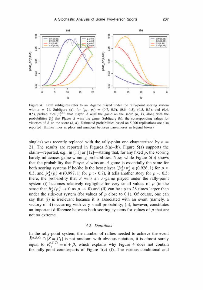
Figures 4(a)–(b) plot the same score distribution curves as in Figures 1(a)–(b),respectively, but in the case of an A-game played under the rally-point scoringsystem with n = 21. Both pairs of plots look roughly similar, althoughextreme scores seem to be less likely in the rally-point scoring; this confirmsthe findings from [11] according to which shutouts are less frequent underthe rally-point scoring system. Note also that, unlike for the side-out scoring,the (pa, pb) = (0.5, 0.5) curve in Figure 4(a) is the exact reverse image ofthe corresponding one in Figure 4(b): for the rally-point scoring, Player A ofcourse does not get any advantage from serving first if (pa, pb) = (0.5, 0.5),which is confirmed by the game-winning probabilities pA

A = pBA = 0.5.

Again, the dependence of the game-winning probabilities on (pa, pb) is ofprimary importance. We will investigate this dependence visually and compareit with the corresponding dependence for the side-out scoring system. To doso, we focus on the no-server version (p = pa = 1 − pb) of Badminton,where, as already mentioned, the side-out scoring system with n = 15 (men’s


Figure 4. Both subfigures refer to an A-game played under the rally-point scoring systemwith n = 21. Subfigure (a): for (pa, pb) = (0.7, 0.5), (0.6, 0.5), (0.5, 0.5), and (0.4,0.5), probabilities pn,k,A

A that Player A wins the game on the score (n, k), along with theprobabilities pA

A that Player A wins the game. Subfigure (b): the corresponding values forvictories of B on the score (k, n). Estimated probabilities based on 5,000 replications are alsoreported (thinner lines in plots and numbers between parentheses in legend boxes).

singles) was recently replaced with the rally-point one characterized by n =21. The results are reported in Figures 5(a)–(b). Figure 5(a) supports theclaim—reported, e.g., in [11] or [12]—stating that, for any fixed p, the scoringbarely influences game-winning probabilities. Now, while Figure 5(b) showsthat the probability that Player A wins an A-game is essentially the same forboth scoring systems if he/she is the best player ( pA

A/pAA ∈ (0.926, 1) for p ≥

0.5, and pAA/pA

A ∈ (0.997, 1) for p > 0.7), it tells another story for p < 0.5:there, the probability that A wins an A-game played under the rally-pointsystem (i) becomes relatively negligible for very small values of p (in thesense that pA

A/pAA → 0 as p → 0) and (ii) can be up to 28 times larger than

under the side-out system (for values of p close to 0.1). Of course, one cansay that (i) is irrelevant because it is associated with an event (namely, avictory of A) occurring with very small probability; (ii), however, constitutesan important difference between both scoring systems for values of p that arenot so extreme.

4.2. Durations

In the rally-point system, the number of rallies needed to achieve the eventEα,β,C2 ∩ [S = C1] is not random: with obvious notation, it is almost surelyequal to eα,β,C2

C1= α + β, which explains why Figure 4 does not contain

the rally-point counterparts of Figure 1(c)–(f). The various conditional and


Figure 5. As a function of p = pa = 1 − pb (hence, in the no-server model), probabilitiesp15,k,A

A (in blue) that Player A wins an n = 15 side-out A-game on the score (15,k), alongwith the probabilities p21,k,A

A (in red) that Player A wins an n = 21 rally-point A-game on thescore (21,k). Expectations (first row) and standard deviations (second row) of the numberof rallies needed to complete the corresponding games, unconditional on the winner (firstcolumn), conditional on a victory of Player A (second column), and conditional on a victoryof Player B (third column). Estimated probabilities, expectations, and standard deviations(based on 200 replications at each value of p = 0, 0.0005, 0.0010, 0.0015, . . . , 0.9995) arealso reported (thinner lines).


unconditional means and variances of the number of rallies in the rally-pointsystem (that is, the quantities eA

C , vAC , eC , vC , eA, vA, e, v) can then be readily

computed from the game-winning probabilities given in Theorem 4, in theexact same way as in (4)–(6) for the side-out scoring system. More generally,the corresponding distribution of the number of rallies in a game triviallyfollows from the same game-winning probabilities.

Figures 5(c)–(h) plot, as functions of p = pa = 1 − pb (hence, in theno-server model), expected values and standard deviations of the numbers ofrallies needed to complete (i) A-games played under the side-out system withn = 15 and (ii) A-games played under the rally-point system with n = 21.Clearly, those plots allow for an in-depth (original) comparison of both scoringsystems. Let us first focus on durations unconditional on the winner of thegame. Figure 5(c) shows that games played under the side-out system will lastlonger than those played under the rally-point one for players of roughly thesame level (which was expected because the side-out system will then leadto many exchanges), whereas the opposite is true when one player is muchstronger (which is explained by the fact that shutouts require more ralliesin the rally-point scoring considered than in the side-out one). Maybe lessexpected is the fact (Figure 5(f)) that the standard deviation of D is, uniformlyin p ∈ (0, 1), smaller for the rally-point scoring system than for the side-outsystem, which shows that the transition to the rally-point system indeed makesthe length of the game more predictable. The twin-peak shape of both standarddeviation curves is even more surprising. Finally, note that, while the rally-pointcurves in Figures 5(c) and (f) are symmetric about p = 0.5, the side-outcurves are not, which is due to the server-effect. This materializes into thelimits of eA given by 16 and 15 as p → 0 and p → 1, respectively (which wasexpected: if Player B wins each rally with probability one, he/she will indeedneed 16 rallies to win an A-game, because he/she has to regain the right toserve before scoring his/her first point), but also translates into (i) the fact thatthe mode of the side-out curve in Figure 5(c) is not exactly located in p = 0.5and (ii) the slightly different heights of the two local (side-out) maxima inFigure 5(f).

We then turn to durations conditional on the winner of the game, whoseexpected values and standard deviations are reported in Figures 5(d), (e), (g),and (h). These figures look most interesting and reveal important differencesbetween both scoring systems. Even the general shape of the curves there areof a different nature for both scorings; for instance, the rally-point curves inFigures 5(d)–(e) are monotonic, while the side-out ones are unimodal. Similarly,in Figure 5(g), the rally-point curve is unimodal, whereas the side-out curveexhibits a most unexpected bimodal shape. It is also interesting to look at limitsas p → 0 or p → 1 in those four subfigures; these limits, which are derived inAppendix A.3, are plotted as short horizontal lines. Consider first limits aboveevents occurring with probability one, that is, limits as p → 1 in Figures 5(d),


(g) and limits as p → 0 in Figures 5(e), (h). The resulting limits are totally inline with our intuition: the four conditional standard deviations go to zero,which implies that the limiting conditional distribution of D simply is almostsurely equal to the corresponding limiting (conditional) expectations. The latterthemselves assume very natural values: for instance, for the same reason asabove, eB

A converges to 16, which is therefore the limit of D in probability.Much more surprising is what happens for limits above events occurring

with probability zero, that is, limits as p → 0 in Figures 5(d), (g) and limits asp → 1 in Figures 5(e), (h). Focusing first on the side-out scoring system, it isseen that a (miraculous) victory of A will require, in the limit, almost surelyD = 15 points, while the limiting conditional distribution of D for victories ofB is nondegenerate. The latter distribution is shown (see Appendix A.3) tobe uniform over {n + 1, n + 2 , . . . , 2n} (hence is stochastically bounded!),which is compatible with the values n + 1 + (n − 1)/2(≈3n/2) and (n −1)2/12 for the limiting expectation and variance, respectively. It should benoted here that this huge difference between those two limiting conditionaldistributions of D is entirely due to the server-effect. In the absence of theserver-effect, the Figures 5(e) and (h) should indeed be the exact reverseimage of the Figures 5(d) and (g), respectively. Similarly, the bimodality of theside-out curve in Figure 5(g) is also due to the server-effect. We then considerthe rally-point scoring, which is not affected by the server-effect, so that it issufficient to consider at the limits as p → 0 in Figures 5(d), (g). There, one alsogets a nondegenerate limiting conditional distribution for D, with expectation2n2/(n + 1)(≈2n) and variance 2n2(n − 1)/[(n + 1)2(n + 2)](≈2).

5. Simulations

We performed several Monte Carlo simulations, one for each figure consideredso far (except Figure 2, as it already contains many theoretical curves). Todescribe the general procedure, we focus on the Monte Carlo experimentassociated with the side-out scoring system in Figure 5 (results for therally-point scoring system there or for the other figures are obtained similarly).For each of the 1,999 values of p considered in Figure 5, the correspondingvalues of pA

A(p), eA(p), vA(p), eCA(p), vC

A (p), C ∈ {A, B}, were estimated onthe basis of J = 200 independent replications of an A-game played under theside-out scoring system with pa = 1 − pb = p. Of course, for each fixed p,the game-winning probability pC

A (p) is simply estimated by the proportion ofgames won by C in the J corresponding A-games:

pCA (p) := J C

J:= 1

J

J∑j=1

I Cj ,


where I Cj , j = 1, . . . , J , is equal to one (respectively, zero) if Player C

won (respectively, lost) the j th game. The corresponding estimates foreA(p), vA(p), eC

A(p), and vCA (p) then are given by

eA(p) := 1

J

J∑j=1

d j vA(p) := 1

J

J∑j=1

(d j − eA(p))2,

eCA(p) := 1

J C

J∑j=1

d j I Cj , and vC

A (p) := 1

J C

J∑j=1

(d j − eC

A(p))2

I Cj , (7)

where dj, j = 1, . . . , J , is the total number of rallies in the j th game. Theseestimates are plotted in thin blue lines in Figure 5. Clearly, these simulationsvalidate our theoretical results in Figures 5(a), (c), and (f). To describe whathappens in the other plots, consider, e.g., Figure 5(g). There, it appears that thetheoretical results are confirmed for large values of p only. However, this issimply explained by the fact that for small values of p, the denominator of vA

A(p)(see (7)) is very small. Actually, among the 542 × 200 A-games associatedwith the 542 values of p ≤ 0.2710, not a single one here led to a victory of A,so that the corresponding estimates vA

A(p) are not even defined. Of course,values of p slightly larger than 0.2710 still give rise to a small number ofvictories of A, so that the corresponding estimates vA

A(p) are highly unreliable.The situation improves substantially as p increases, as it can be seen in Figure5(g). Figures 5(b), (d), (e), and (h) can be interpreted exactly in the same way.

This underlines the fact that expectations and variances conditional onevents with small probabilities are extremely difficult—if not impossible—toestimate. To quantify this, let us focus again on Figure 5(g), and consider thelocal maximum on the left of the plot, which is (on the grid of values of p athand) located in p0 := 0.0085. The probability pA

A(p0) of a victory of A in anA-game played under the side-out scoring system with p = p0 is about 3.5 ×10−31. Estimating vA

A(p0) with the same accuracy as that achieved for, e.g.,vA

A(0.5) in Figure 5(g) would then require a number of replications of (fixed p0)A-games that is about 200 × pA

A(0.5)/pAA(p0) ≈ 3 × 1032. Assuming that 106

replications can be performed in a second by a super computer (which is overlyoptimistic), this estimation of vA

A(p0) would still require not less than 9.5 ×1018 years! This means that it is indeed impossible to estimate in a reliableway the conditional variance curve for p close to p0 so that Monte Carloexperiments cannot reveal the existence of the local maximum in p0. Similarly,without our theoretical analysis, there is no hope to learn about the degeneracy(respectively, nondegeneracy) of the limiting distribution of D conditional on avictory of A as p → 0 (respectively, conditional on a victory of B as p → 1).

We will not comment in detail the Monte Carlo results associated with theother figures. We just report that they again confirm our theoretical findings,


whenever possible, that is, whenever they are not associated with conditionalresults above events with small probabilities.

6. Conclusion and final comments

This paper provides a complete rally-level probabilistic description for gamesplayed under the side-out scoring system. It complements the previous maincontributions from [7, 10] and [11] by adding to the well-known game-winningprobabilities an exhaustive knowledge of the random duration of the game.This brings a much better understanding of the underlying process as a whole,as is demonstrated in Sections 2 to 4.

In this final section, we will mainly focus on the practical implicationsof our findings. For this, we may restrict to (pa, pb) ∈ [0.4, 0.6] × [0.4,0.6], say, because players tend to be grouped according to strength. For suchvalues of the rally-winning probabilities, our results show that the recenttransition—in men’s singles’ Badminton—from the n = 15 side-out scoringsystem to the n = 21 rally-point one strongly affected the properties of thegame. They indeed indicate that games played under the rally-point scoringsystem are much shorter than those played according to the side-out one, andthat the uncertainty in the duration of the match is significantly reduced. Ourresults allow quantifying both effects. On the other hand, they show thatgame-winning probabilities are essentially the same for both scoring systems.It is then tempting to conclude (as in [11, 12]) that the outcomes of the gamesare barely influenced by the scoring system adopted. While this is strictlyvalid in the model, it is highly disputable under possible violations of themodel. For instance, i.i.d.-ness (see page 2) may fail to hold for long gamesinvolving players with different fitness levels, a violation of the model underwhich scoring systems, through their impact on the duration of the games (seeabove), may significantly influence the outcomes of the games.

In practice, the results of this paper can be useful to many actors of the sportcommunity. For the international sport federations playing with the idea ofreplacing the side-out scoring system with the rally-point one, our results couldbe used to tune n (i.e., the number of points to be scored to win a rally-pointgame) according to their wishes. For the sake of illustration, consider again thetransition performed by the International Badminton Federation. Presumably,its objective was (i) to make the duration of the game more predictable and (ii)to ensure that the outcome of the matches would change as little as possible. Ifthis was indeed the objective, then our results show that it has only beenpartially achieved: it is indeed easy to see that other choices of n would havebeen even better in that respect, the choice of n = 27 (see Figure 6(b) and (d)),being optimal. Moreover, this last choice would have affected the duration ofthe game much less than n = 21 (see Figure 6(c)), and thus would have


Figure 6. Subfigures (a)–(e) here report Subfigures (a)–(c), (f), and (e) from Figure 5 withthe only difference that the rally-point scoring here is based on n = 27 (the side-out scoring isstill based on n = 15).

made the outcome of the matches more robust to possible violations of themodel.

For organizers of local tournaments played under the side-out scoringsystem, our results can be used to control, for any fixed number of plannedmatches, the time required to complete their events. Such a control over thisrandom time, at any fixed tolerance level, can indeed be achieved in a quitedirect way from our results on the duration of a game played under the side-outscoring system. Organizers can then deduce, at the corresponding tolerancelevel, the number of matches—hence the number of players—their events willbe able to host. This of course concerns the sports that are still using thisscoring system, such as racquetball and squash (for the latter, only in countriescurrently using the so-called English scoring system).


Finally, because our results provide a complete description of the durationprocess in the side-out scoring system, they also open the way to more efficientestimation of the rally-winning probabilities (pa, pb) there. However, a fulldiscussion of this is beyond the scope of this paper, and is actually the topic ofcurrent research [8].

Appendix: proofs

A.1. Proofs of Lemma 1 and Theorem 1

In the Appendix, we simply write interruptions for A-interruptions.

Proof of Lemma 1. Clearly, pα,β,AA (r, j) = Kr, j pα

a pβ

b (qaqb)r+ j , where K r,j

is the number of ways of setting r interruptions and j exchanges in the sequenceof rallies achieving the event under consideration. Regarding interruptions, weargue as in [2], and say those r interruptions should be put into the α possiblespots (remember the last point should be won by A), while the β points scoredby B should be distributed among those r interruptions—with at least onepoint scored by B in each interruption (so that there may be at most r =min (α, β) interruptions). There are exactly (αr )(β−1

r−1) ways to achieve this. As

for the j exchanges, they may occur at any time and thus there are as manyways of placing j interruptions as there are distributions of j indistinguishable

balls into α + β urns, i.e., (α+β−1j ). Summing up, we have proved that

pα,β,AA (r, j) =

(α + β − 1

j

)(α

r

)(β − 1

r − 1

)pα

a pβ

b (qaqb)r+ j ,

with r = min(β, 1), . . . , min(α, β), j ∈ N.As for pα,β,B

A (r, j), this probability is clearly of the form Lr, j pαa pβ

b qa ×(qaqb)r+ j−1. In this case, there are α + 1 possible spots for the r interruptions.However, because B scores the last point, the sequence of rallies should end

with an interruption. There are therefore ( αr−1) ways to insert the interruptions.

Each interruption contains at least one point for B, so that r ≤ min (α + 1, β).

The result follows by noting that there are (β−1r−1) ways of distributing the β

points scored by B into those r interruptions, and by dealing with exchangesas for pα,β,A

A (r, j). �

Proof of Theorem 1. The result directly follows from Lemma 1 by writingpα,β,A

A = ∑r, j pα,β,A

A (r, j) and pα,β,BA = ∑

r, j pα,β,BA (r, j) (where the sums are

over all possible values of r and j in each case), and by using the equality∑∞j=0(m+ j−1

j )z j = (1 − z)−m for any z ∈ [0, 1). �


A.2. Proofs of Theorems 2 and 3 and of Corollary 1

Proof of Theorem 2. First note that if A scores the last point in an A-gamein which the score is α to β after j exchanges ( j ∈ {0, 1, . . . }) and rinterruptions (r ∈ {γ 0, . . . , γ 1}), then there have been α + β + 2(r + j) rallies.Conditioning on the number of interruptions and exchanges therefore yields

Mα,β,AA (t) = (

pα,β,AA

)−1∑j

∑r

et(α+β+2(r+ j)) pα,β,AA (r, j)

(where the sums are over all possible values of r and j in each case) and thus,from Lemma 1 and Theorem 1,

Mα,β,AA (t) =

et(α+β)∑

j

(e2tq) j

(α + β + j − 1

j

)∑r

e2tr

(α

r

)(β − 1

r − 1

)qr

(1 − q)−(α+β)∑

r

(α

r

)(β − 1

r − 1

)qr

= ((1 − q)et

)α+β

( ∑j

(e2tq) j

(α + β + j − 1

j

))

×(∑

r

e2tr W α,β,AA (q, r )

).

The first claim of Theorem 2 follows.For the second claim, it suffices to note that if B scores the last point in an

A-game in which the score is of α to β after j exchanges ( j ∈ {0, 1, . . . }) andr interruptions (r ∈ {1, . . . , γ 2 + 1}), then the number of rallies equals α +β + 2(r − 1 + j) + 1; the computations above then hold with only minorchanges. �

Proof of Corollary 1. Taking first and second derivatives of the momentgenerating functions yields the expectations and variances given in Corollary 1.Moreover it can easily be seen that derivatives of the expected values withrespect to q are positive by using the Cauchy–Schwarz inequality, and thus thelatter are strictly monotone increasing in q. �

Proof of Theorem 3. The change of variables z = et in the momentgenerating functions given in Theorem 2 immediately yields the probabilitygenerating functions. If β = 0, the latter is already in the form of an infinite

series Gα,0,AA (z) = ∑∞

j=0(1 − q)αq j (α+ j−1j )zα+2 j . If β > 0, we have

Gα,β,AA (z) = (1 − q)α+βzα+β

∞∑j=0

K j z2 j

γ1∑r=1

Wr z2r ,


where K j = q j (α+β+ j−1j ) and Wr = W α,β,A

A (q, r ). This double sum satisfies

∞∑j=0

K j

γ1∑r=1

Wr z2( j+r ) =γ1∑

j=1

z2 j

(j−1∑l=0

Kl W j−l

)+

∞∑j=γ1+1

z2 j

⎛⎝ j−1∑

l= j−γ1

Kl W j−l

⎞⎠ .

The same arguments are readily adapted to Gα,β,BA (z), and Theorem 3

follows. �

A.3. The distribution of the number of rallies, in the no-server model,for extreme rally-winning probabilities

As announced in Section 4.2, we determine here the limiting behavior of thenumber of rallies D, in the no-server model, for p → 0 and p → 1, conditionalon the winner of the A-game considered. We start with the limit under almostsure events, that is, limits as p → 1 (respectively, p → 0) for the distributionof D conditional on a victory of A (respectively, of B).

PROPOSITION 1. Let, for the side-out scoring system, t �→ MCA (t) =

E[et D | EC , S = A], C ∈ {A, B}, be the moment generating function of Dconditional on the event EC ∩ [S = A]. Denote by t �→ MC

A (t) = E[et D | EC ,

S = A], C ∈ {A, B}, the corresponding moment generating function for therally-point system. Then, (i) as p → 1, M A

A (t) → ent and M AA (t) → ent ; (ii) as

p → 0, M BA (t) → e(n+1)t and M B

A (t) → ent .

Proof . (i) By conditioning, we get M AA (t) = ∑n−1

k=0 Mn,k,AA (t)pn,k,A

A /pAA . It is

easy to check that limp→1 pn,k,AA /pA

A = δk,0 and that limp→1 Mn,k,AA (t) = e(n+k)t .

Hence limp→1 M AA (t) = ent . Likewise, M A

A (t) = ∑n−1k=0 e(n+k)t pn,k,A

A / pAA . Again,

it is easy to check that limp→1 pn,k,AA / pA

A = δk,0. Hence, we indeed haveM A

A (t) → ent . (ii) The proof is similar, and thus left to the reader. �

COROLLARY 2. (i) As p → 1, (eAA, vA

A) → (n, 0) and (eAA, vA

A) → (n, 0), so

that, conditional on a victory of A in an A-game, DP→ n, irrespective of

the scoring system; (ii) as p → 0, (eBA, vB

A ) → (n + 1, 0) and (eBA, vB

A ) →(n, 0), so that, conditional on a victory of B in an A-game, D

P→ n + 1(respectively, n) for the side-out (respectively, rally-point) scoring system.

As shown by Proposition 1 and Corollary 2, the situation is here very clear.In each of the four cases considered, only one trajectory is possible, namelythat for which all rallies in the game will be won by the winner of the game.

Next we derive the limiting conditional distribution of D under events whichoccur with zero probability, that is, limits as p → 1 (respectively, p → 0) for


the distribution of D conditional on a victory of B (respectively, of A). Ourconclusions are much more surprising.

PROPOSITION 2. Let m(t) := ∑n−1k=0 e(n+k)t (n+k−1

k )/∑n−1

k=0(n+k−1k ). Then, (i)

as p → 0, M AA (t) → ent and M A

A (t) → m(t); (ii) as p → 1, M BA (t) →

(e(n+1)t − e(2n+1)t )/(n(1 − et )) and M BA (t) → m(t). In particular, as p → 1,

the limiting distribution of D conditional on the event E B ∩ [S = A] isuniform over the set {n + 1, . . . , 2n}.

Proof . We first prove the assertions for the rally-point scoring system.In this case, M A

A (t) = ∑n−1k=0 e(n+k)t pn,k,A

A / pAA . Now, from Remark 1 it is

immediate that limp→0 pn,k,AA /pA

A = (n+k−1k )/

∑n−1k=0(n+k−1

k ), which proves the

claim for M AA (t) (hence, by symmetry, also for M B

A (t)).Next consider the assertions for the side-out scoring system. First note that,

as before, M AA (t) = ∑n−1

k=0 Mn,k,AA (t)pn,k,A

A /pAA and M B

A (t) = ∑n−1k=0 Mk,n,B

A (t)pk,n,B

A /pBA . Now fix k ∈ {0, . . . , n − 1}. Using Theorem 1, one readily shows

that

limp→0

pn,k,AA

/pA

A = δk,0 and limp→1

pk,n,BA

/pB

A = 1/n.

Combining these results and the definitions of the moment generating functions,it is then straightforward to show that

limp→0

Mn,k,AA (t) = e(n+k)t and lim

p→1Mk,n,B

A (t) = e(n+k+1)t .

The claim follows. �

COROLLARY 3. (i) As p → 0, (eAA, vA

A) → (n, 0) and (eAA, vA

A ) → ( 2n2

n+1 ,2n2(n−1)

(n+1)2(n+2) ); as p → 1, (eBA, vB

A ) → ( 3n+12 ,

(n−1)2

12 ) and (eBA, vB

A ) → ( 2n2

n+1 ,

2n2(n−1)(n+1)2(n+2) ).

It is remarkable that we can again give a complete description of the“distribution of the process” (by this, we mean that we can again list alltrajectories of rallies leading to the event considered, and give, for eachsuch trajectory, its probability). Consider first the side-out scoring system.For victories of A, the situation is very clear: Corollary 2 indeed yields that,

conditional on a victory of A in an A-game, DP→ n as p → 0, which implies

that the only possible trajectory of rallies is the one for which all rallies in thegame are won by A. Turn then to victories of B. There, we obtained in theproof of Proposition 2 that all scores (k, n) are equally likely. It is actually

easy to show that, conditional on Ek,n,B ∩ [S = A], DP→ n + k + 1 as p →

1. This implies that there are exactly n equally likely trajectories: A first scores


k points, then loses his/her serve, before B scores n (miraculous) points andwins the game (k = 0, . . . , n − 1).

Consider finally the rally-point system. In this case, it is sufficient to studythe distribution of the scores after victories of A (when p → 0) because thenumber of rallies is a function of the scores only, and because the conclusionswill, by symmetry, be identical for victories of B (when p → 1). Clearly,

for any fixed k ∈ {0, 1, . . . , n − 1}, there are exactly (n+k−1k ) trajectories

leading to the score (n, k), and those trajectories are equally likely. Each such

trajectory will then occur with probability 1/∑n−1

k=0(n+k−1k ), because, as we have

seen in the proof of Proposition 2, the score (n, k) occurs with probability

(n+k−1k )

/ ∑n−1k=0(n+k−1

k ). These considerations provide the whole distribution of

the process: there are∑n−1

k=0(n+k−1k ) equally likely possible trajectories, namely

the ones we have just considered. The exact limiting distribution of D can ofcourse trivially be computed from this.

Acknowledgments

The research of Davy Paindaveine (who is also member of ECORE, theassociation of CORE and ECARES) is supported by an A.R.C. contract ofthe Communaute Francaise de Belgique; and that of Yvik Swan is supportedby a Mandat de Charge de Recherche from the Fonds National de laRecherche Scientifique, Communaute francaise de Belgique. The authors thankan anonymous referee for insightful comments and suggestions that led to asignificant improvement of the paper.

References

1. C. L. ANDERSON, Note on the advantage of first serve, J. Combin. Theory Ser. A 23:363(1977).

2. F. J. G. M. KLAASSEN and J. R. MAGNUS, Forecasting the winner of a tennis match,European J. Oper. Res. 148:257–267 (2003).

3. P. K. NEWTON and J. B. KELLER, Probability of winning at tennis I. Theory and data,Stud. Appl. Math. 114:241–269 (2005).

4. R. S. SCHULMAN and M. A. HAMDAN, A probabilistic model for table tennis, Canad. J.Statist. 5:179–186 (1977).

5. P. K. NEWTON and K. ASLAM, Monte Carlo Tennis, SIAM Rev. 48:722–742 (2006).6. B. P. HSI and D. M. BURICH, Games of two players, J. Roy. Statist. Soc. Ser. C 20:86–92

(1971).7. M. J. PHILLIPS, Sums of random variables having the modified geometric distribution

with application to two-person games, Adv. Appl. Probab. 10:647–665 (1978).8. J. B. KELLER, Probability of a shutout in racquetball, SIAM Rev. 26:267–268 (1984).


9. D. J. MARCUS, Probability of winning a game of racquetball, SIAM Rev. 27:443–444(1985).

10. D. STRAUSS and B. C. ARNOLD, The rating of players in racquetball tournaments, J. Roy.Statist. Soc. Ser. C 36:163–173 (1987).

11. J. SIMMONS, A probabilistic model of squash: strategies and applications, J. Roy. Statist.Soc. Ser. C 38:95–110 (1989).

12. D. F. PERCY, A mathematical analysis of badminton scoring systems, J. Oper. Res. Soc.60:63–71 (2009).

13. J. RENICK, Optional strategy at decision points, Res. Quart. 47:562–568 (1976).14. J. RENICK, Tie point strategy in badminton and international squash, Res. Quart.

48:492–498 (1977).

UNIVERSITE LIBRE DE BRUXELLES, BELGIUM

(Received August 1, 2010)

a stochastic analysis of some two-person sports sapm... · a stochastic analysis of some two-person...

Documents