A Step-by-Step Guide to Survival Analysis Lida Gharibvand, University of California, Riverside

ABSTRACT Survival analysis involves the modeling of time-to-event data whereby death or failure is considered an "event". The graphical presentation of survival analysis is a significant tool to facilitate a clear understanding of the underlying events. In particular, the graphical presentation of Cox’s proportional hazards model using SAS PHREG is important for data exploration in survival analysis. In this paper, we will present a comprehensive set of tools and plots to implement survival analysis and Cox’s proportional hazard functions in a step-by-step manner. We will demonstrate the features of SAS ® PROC LIFEREG, PROC LIFETEST, PROC PHREG, PROC BPHREG, estimated hazard function, survival function, advanced features of PHREG, and selecting the best candidate models in model selection. A method will be outlined to perform all possible subset model selection within user-defined subsets using AIC information criterion. The new user-friendly features of BPHREG, an experimental upgrade to PHREG procedure, such as ‘class’, ‘hazards ratio’, and ‘strata’ statements will be covered. The cumulative residuals from PROC PHREG are used to investigate the model specification error of covariate and validate the proportion hazard function. Finally, the methods to identify outliers are commonly based on Cox regression residuals such as Martingale and deviance residuals which will be demonstrated using PROC GPLOT in SAS/GRAPH.

INTRODUCTION Survival analysis is the phrase used to describe the analysis of data in the form of times from a well-defined “time origin” until the occurrence of some particular event or “end-point”. In medical research, the time origin often corresponds to the recruitment of an individual into an experimental study, such as a clinical trial to compare two or more treatments. This in turn may coincide with the diagnosis of a particular condition, the commencement of a treatment regiment, or the occurrence of some adverse event. If the end point is the death of a patient, the resulting data are literally survival times. However, data of a similar form can be obtained when the end-point is not fatal, such as the relief of pain, or the recurrence of symptoms. In this case, the observations are often referred to as time to event data. The analysis of survival data requires special techniques because the data are almost always incomplete and familiar parametric assumptions may be unjustifiable. Investigators follow subjects until they reach a pre-specified endpoint (for example, death). However, subjects sometimes withdraw from a study, or the study is completed before the endpoint is reached. In these cases, the survival times (also known as failure times) are censored; subjects survived to a certain time beyond which their status is unknown. The uncensored survival times are sometimes referred to as event times. Methods for survival analysis must account for both censored and uncensored data. This paper is focusing on PROC LIFEREG, PROC LIFETEST, PROC PHREG and PROC BPHREG which are important tools to analyze survival data. This paper also demonstrates some sophisticated graphics made possible by the new SAS ODS Statistical Graphics capability.

SURVIVAL DATA The actual data from Mayo liver disease example of Lin, Wei, and Ying (1993) is used here to demonstrate the features. The data consists of 418 patients with Primary Biliary Cirrhosis (PBC), among which 161 had died as of the date of data listing. The data set contains the following variables: Time Follow-up time in years Censor Event indicator with value 1 for death time and value 0 for censored time Age Age in years from birth to study registration Alb Serum albumin level in gm/dl Bili Serum Bilirubin level in mg/dl Edema Edema with value 0 for presence of no Edema, Edema with value 0.5 for untreated or successfully treated, and Edema with value 1 for unsuccessfully treated Edema Protime Prothrombin time in seconds

1

SAS PROCS: There are three important SAS procedures available for analyzing survival data: LIFEREG, LIFETEST and PHREG (BPHREG). PROC LIFEREG is a parametric regression procedure for modeling the distribution of survival time with a set of concomitant variables (SAS Institute, Inc. (2007a)). PROC LIFETEST is a nonparametric procedure for estimating the survivor function, comparing the underlying survival curves of two or more samples, and testing the association of survival time with other variables (SAS Institute, Inc. (2007b)). PROC PHREG is a semi-parametric procedure that fits the Cox proportional hazards model (SAS Institute, Inc. (2007c)). PROC BPHREG is an experimental upgrade to PHREG procedure that can be used to fit Bayesian Cox proportional hazards model (SAS Institute, Inc. (2007d)).

PROC LIFEREG The LIFEREG procedure fits parametric accelerated failure time models to survival data that may be left, right, or interval censored. The parametric model is of the form

σεβ +′= Xy where y is usually the log of the failure time variable, x is a vector of covariate values, β is a vector of unknown regression parameters, σ is an unknown scale parameter, and ε is an error term. The distribution of the random disturbance can be taken from a class of distributions that includes the extreme value, normal, logistic, and, by using a log transformation, the exponential, Weibull, lognormal, loglogistic, and three-parameter gamma distributions. These models are equivalent to accelerated failure time models when the log of the response is the quantity being modeled. The accelerated failure time model assumes a parametric form for the effects of the explanatory variables and usually assumes a parametric form for the underlying survivor function that the effect of covariates on an event time distribution is multiplicative on the event time. The LIFEREG Procedure can be also used to perform a Tobit analysis, a regression model for left-censored data assuming a normally distributed error term. For more information on LIFEREG refer the SAS Institute on-line documentation (SAS Institute, Inc. (2007a)). There is no ODS Graphics feature available in PROC LIFEREG (version 9.1.3). However we can generate the survival probability plot using the PROBPLOT option. The following example demonstrates how you can use the LIFEREG procedure to fit a parametric model to failure time data. Consider fitting the survival time of the PBC patients with covariates Bili, log(Protime), log(Alb), Age and Edema. The log transform, which is often applied to blood chemistry measurements, is deliberately not employed for Bili. It is of interest to assess the functional form of the variable Bili in the failure time data model. Please refer to Code Box 1.

ODS RTF FILE='path\filename.rtf'style=statistical; ODS LISTING CLOSE; DATA pbc; GOPTIONS RESET=all COLORS=(Black, RED,BLUE,YELLOW,GREEN,MAGENTA,CYAN) dev=EMF target=EMF XMAX=7 YMAX=7 HTEXT=14pt FTEXT="<ttf> Arial";

PROC LIFEREG DATA=pbc; CLASS Edema; MODEL time*Censor(0)= Age logAlb logProtime Bili Edema; PROBPLOT Cencolor=red cframe=ligr cfit=blue ppout npintervals=simul; INSET / cfill = white ctext = blue; RUN;

Code Box 1: PROC LIFEREG Code The PROC LIFEREG statement invokes the LIFEREG procedure. The MODEL statement is required and specifies the variables used in the regression part of the model as well as the distribution used for the error, or random, component of the model (The default distribution used is Weibull and this can be changed for a better fit). Only a single MODEL statement can be used with one invocation of the LIFEREG procedure. If multiple MODEL statements are present, only the last model is used. Main effects and interaction terms can be specified in the MODEL statement, similar to the GLM procedure. Initial values can be specified in the MODEL statement or in an INEST= data set. If no initial values are specified, the starting estimates are obtained by ordinary least squares. Categorical variables can be specified in CLASS statement. Survival probability plot can be generated with PROBPLOT. Executing the code above will produce the following plot.

2

Follow-up Tim e in Years

Per

cen

t

.1 1 10 100

.1

.2

.5

1

2

5

10

20

304050

80

95

99Uncensored 161Right Censored 257Shape 1.421Conf. Level 95%Distribu tion W eibu ll

Figure 1: Survival Plot Produced by LIFEREG Procedure

The resulting graphical output is shown in Figure 1. The estimated CDF, a line representing the maximum likelihood fit, and point wise parametric confidence bands are plotted here. The values of right-censored observations are plotted along the top of the graph. Figure 1 assesses the quality of the model fit. As we can see, the model fit is not very satisfactory. We will show how to improve the model fit in this paper.

PROC LIFETEST The LIFETEST procedure can be used to compute nonparametric estimates of the survivor function either by the product-limit method (also called the Kaplan-Meier method) or by the life-table method (also called the actuarial method), comparing the underlying survival curves of two or more samples, and testing the association of survival time with other variables. PROC LIFETEST provides non-parametric k-sample tests based on weighted comparisons of the estimated hazard rate of the individual population under the null and alternative hypotheses. This proc also computes the rank tests and a likelihood ratio test for testing the homogeneity of survival functions across strata. The ODS GRAPHICS features are available in PROC LIFETEST. ODS GRAPHICS ON will add statistical graphics to the output. The simplest use of PROC LIFETEST is to request the nonparametric estimates of the survivor function for a sample of survival times. In such a case, only the PROC LIFETEST statement and the TIME statement are required. All statements except the TIME

ODS RTF FILE='path\filename.rtf'style=statistical; ODS LISTING CLOSE; ODS GRAPHICS on; DATA pbc; PROC LIFETEST DATA=pbc; TIME Time*Censor(0); SURVIVAL out=Out1 confband=all bandmin=100 bandmax=600 MAXTIME=800 conftype=asinsqrt PLOTS=(stratum, survival, hwb); STRATA Edema; TEST Age logAlb logProtime Bili; RUN; ODS GRAPHICS OFF; ODS RTF CLOSE; ODS LISTING; QUIT;

Code Box 2: PROC LIFETEST Code

3

All statements except the TIME statement are optional, and there is no required order for the statements following the PROC LIFETEST statement. Please refer to Code Box 2. The PROC LIFETEST procedure generates survival graphs from the PLOTS = (s) option. The legend and long-rank p-value annotations are automatically generated when the STRATA statement is used. To disable the graphics after execution, enter the statement ODS GRAPHICS OFF.

Figure 2: Panel Plot for Patients with Edema=0 (Experimental)

Figure 3: Panel Plot for Patients with Edema=0.5 (Experimental)

4

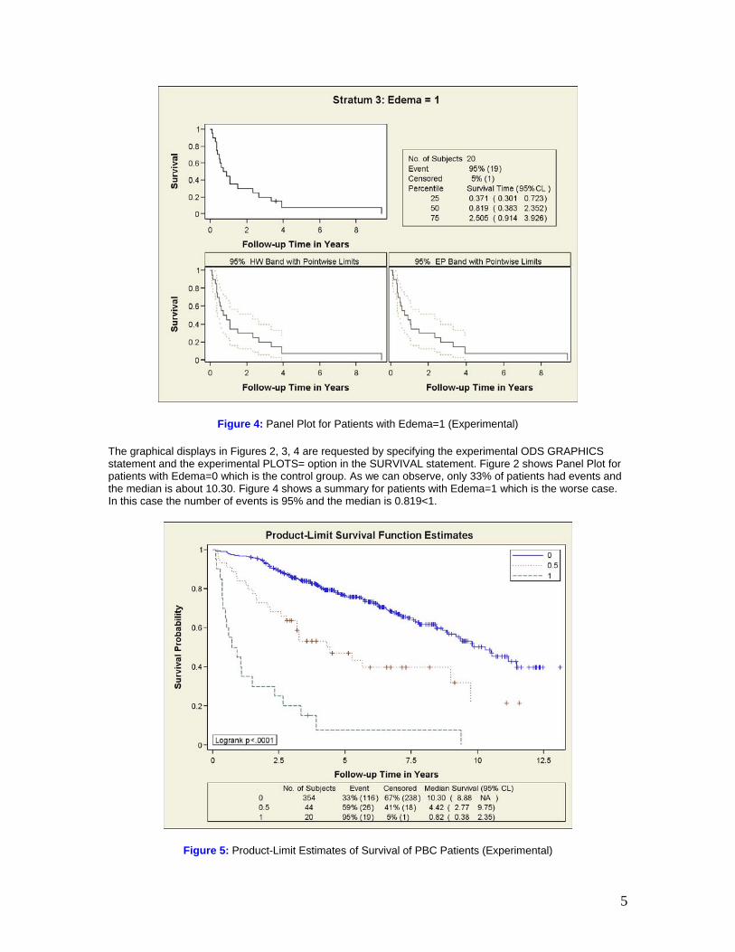
Figure 4: Panel Plot for Patients with Edema=1 (Experimental) The graphical displays in Figures 2, 3, 4 are requested by specifying the experimental ODS GRAPHICS statement and the experimental PLOTS= option in the SURVIVAL statement. Figure 2 shows Panel Plot for patients with Edema=0 which is the control group. As we can observe, only 33% of patients had events and the median is about 10.30. Figure 4 shows a summary for patients with Edema=1 which is the worse case. In this case the number of events is 95% and the median is 0.819<1.

Figure 5: Product-Limit Estimates of Survival of PBC Patients (Experimental)

5

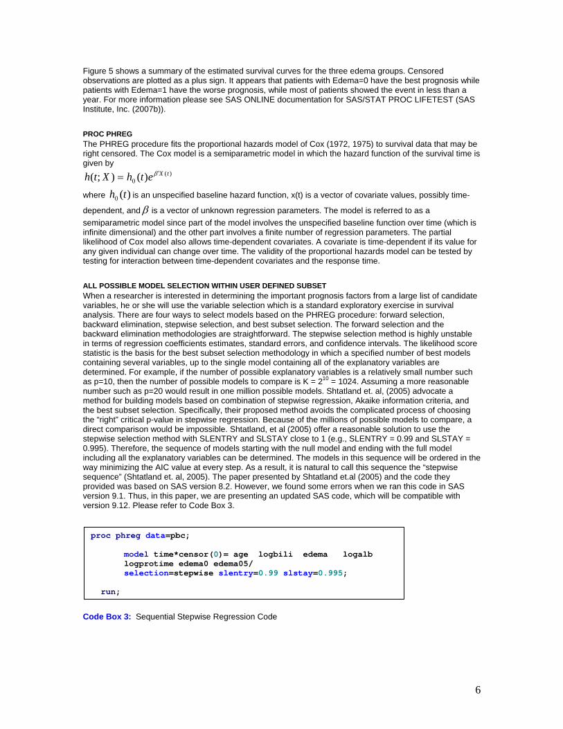
Figure 5 shows a summary of the estimated survival curves for the three edema groups. Censored observations are plotted as a plus sign. It appears that patients with Edema=0 have the best prognosis while patients with Edema=1 have the worse prognosis, while most of patients showed the event in less than a year. For more information please see SAS ONLINE documentation for SAS/STAT PROC LIFETEST (SAS Institute, Inc. (2007b)).

PROC PHREG The PHREG procedure fits the proportional hazards model of Cox (1972, 1975) to survival data that may be right censored. The Cox model is a semiparametric model in which the hazard function of the survival time is given by

)(0 )();( tXethXth β ′=

where is an unspecified baseline hazard function, x(t) is a vector of covariate values, possibly time-

dependent, and

)(0 thβ is a vector of unknown regression parameters. The model is referred to as a

semiparametric model since part of the model involves the unspecified baseline function over time (which is infinite dimensional) and the other part involves a finite number of regression parameters. The partial likelihood of Cox model also allows time-dependent covariates. A covariate is time-dependent if its value for any given individual can change over time. The validity of the proportional hazards model can be tested by testing for interaction between time-dependent covariates and the response time.

ALL POSSIBLE MODEL SELECTION WITHIN USER DEFINED SUBSET When a researcher is interested in determining the important prognosis factors from a large list of candidate variables, he or she will use the variable selection which is a standard exploratory exercise in survival analysis. There are four ways to select models based on the PHREG procedure: forward selection, backward elimination, stepwise selection, and best subset selection. The forward selection and the backward elimination methodologies are straightforward. The stepwise selection method is highly unstable in terms of regression coefficients estimates, standard errors, and confidence intervals. The likelihood score statistic is the basis for the best subset selection methodology in which a specified number of best models containing several variables, up to the single model containing all of the explanatory variables are determined. For example, if the number of possible explanatory variables is a relatively small number such as p=10, then the number of possible models to compare is K = 210 = 1024. Assuming a more reasonable number such as p=20 would result in one million possible models. Shtatland et. al, (2005) advocate a method for building models based on combination of stepwise regression, Akaike information criteria, and the best subset selection. Specifically, their proposed method avoids the complicated process of choosing the “right” critical p-value in stepwise regression. Because of the millions of possible models to compare, a direct comparison would be impossible. Shtatland, et al (2005) offer a reasonable solution to use the stepwise selection method with SLENTRY and SLSTAY close to 1 (e.g., SLENTRY = 0.99 and SLSTAY = 0.995). Therefore, the sequence of models starting with the null model and ending with the full model including all the explanatory variables can be determined. The models in this sequence will be ordered in the way minimizing the AIC value at every step. As a result, it is natural to call this sequence the “stepwise sequence” (Shtatland et. al, 2005). The paper presented by Shtatland et.al (2005) and the code they provided was based on SAS version 8.2. However, we found some errors when we ran this code in SAS version 9.1. Thus, in this paper, we are presenting an updated SAS code, which will be compatible with version 9.12. Please refer to Code Box 3.

proc phreg data=pbc;

model time*censor(0)= age logbili edema logalb logprotime edema0 edema05/ selection=stepwise slentry=0.99 slstay=0.995;

run;

Code Box 3: Sequential Stepwise Regression Code

6

Step Criterion Without Covariates With Covariates

1 AIC 2659.489 2632.123

2 AIC 2659.489 2617.642

3 AIC 2659.489 2617.143

4 AIC 2659.489 2617.952

5 AIC 2659.489 2619.195

6 AIC 2659.489 2621.184

7 AIC 2659.489 2623.172

Table 1: Sequential Stepwise Regression Output

The minimum AIC is obtained in step three with three variables model. Therefore, we can perform all possible subset selection between 2 and 4 subsets (3-1 and 3+1). The SAS code for performing all subset selection between subset 2 and 4 using all combination is provided in Code Box 4.

ods output BestSubsets=Best_subsets;ods rtf exclude all; proc phreg data=pbc; model time*censor(0)=age logbili edema logalb logprotime edema0 edema05 / selection=score START= 2 STOP= 4 ; run; OPTIONS MPRINT SYMBOLGEN MLOGIC; %MACRO SCORE; proc sql noprint; select (nobs -delobs) into: num from dictionary.tables where libname ='WORK' and memname = "BEST_SUBSETS"; run; %let num=&num; %do i=1 %to &num; data _null_ ; set Best_Subsets; if _N_ = &i; call symput('list', VariablesInModel); run; ods output FitStatistics=Fit2; ods rtf exclude all; proc PHREG data=pbc; model time*censor(0) = &list; run; ods rtf select all; data icaic(keep=aic); set fit2; if criterion='AIC'; aic=withcovariates; run; data ic(keep=model aic ); set icaic; model="&list"; Run; run; Proc append base=subaic data=ic force; run; %end; MEND; %SCORE

Code Box 4: All subset selection between subset 2 and 4 using all combinations

7

The results of all possible subset selection within user defined subset out of so many subsets (91) are presented in Table 2. We are only showing the result of ten top models in Table 2. The best model includes four variables: logbili, logalb, logprotime, and edema0.

AIC Model

2617.95 logbili logalb logprotime edema0

2631.19 logbili logalb logprotime

2631.85 Age logbili logalb logprotime

2632.21 logbili edema logalb logprotime

2633.19 logbili logalb logprotime edema05

2664.69 logbili logalb edema0

2665.58 logbili edema logalb edema0

2666.55 Age logbili logalb edema0

2666.68 logbili logalb edema0 edema05

2677.41 logbili edema logalb Table 2: Top ten models selected based on minimum AIC from the subset selection between subset 2 & 4.

PROC PHREG ODS STATISTICAL GRAPHICS FEATURES There is only one ODS GRAPHICS PLOT, cumulative residual plot for detecting model specification error, available in Version 9.1.3. As Lin et al. (1993) suggests, a Cox model for the survival time of the PCB patients with covariates Bili, log(Protime), log(Albumin), Age and Edema was fitted using the following code in Code Box 5.

ODS GRAPHICS on; DATA pbc; PROC PHREG DATA=pbc; MODEL Time*Censor(0)= Bili logAlb logProtime Edema Age; logProtime=log(Protime); logAlb=log(Alb); ASSESS VAR=(Bili) / RESAMPLE; RUN; OUTPUT OUT=outp XBETA=xb RESMART=mart RESDEV=dev RESSCH =ressch LMAX=lmax RESSCO=ressco; ODS GRAPHICS oFF; QUIT;

Code Box 5: Fitting the Survival Time Model

The ASSESS statement creates a plot of the cumulative Martingale residuals against the values of the covariate Bili, which is specified in the VAR= option. The RESAMPLE option computes the p-value of a Kolmogorov-type supremum test based on a sample of 1,000 simulated residual patterns.

8

Figure 6: Cumulative Martingale residuals vs Bili (Experimental)

The plot in Figure 6 displays the observed cumulative Martingale residual process for Bili together with 20 simulated realizations from the null distribution. This graphical display is requested by specifying the experimental ODS GRAPHICS statement and the experimental ASSESS statement.

Figure 7: Typical cumulative residual plot patterns

9

The curve of observed cumulative Martingale residuals in Figure 6 most resembles the behavior of the curve in Figure 7(a), indicating that log(Bili) might be a more appropriate term in the model than Bili. Next, the analysis of the natural history of the PBC is repeated with log(Bilir) replacing Bili, and the functional form of log(Bilir) is assessed (Figure 8). When we compare Figures 6 and 8, we can see that Figure 8 shows a better function form when log(Bilir) was used. Therefore, the model fit is improved when Bili is replaced by log(Bilir).

Figure 8: Cumulative Martingale residuals vs log(Bili)

PROC BPHREG- NEW SAS EXPERIMENTAL PROC In PHREG 9.1.3, there is no CLASS statement and the ASSESS statement fails to produce ODS Graphics in presence of STRATA variable. However, a new experimental PHREG procedure is available to run Bayesian PHREG (BPHREG). In the BPHREG statement we can include CLASS statement and ASSESS statement. Please refer to Code Box 6. Users can download BPHREG at http://www.sas.com/apps/demosdownloads/setupintro.jsp. Then click on SAS/STAT Software and then SAS/STAT Bayesian Procedures to download.

CHECKING FOR PROPORTIONAL HAZARD FUNCTIONS

proc bphreg data=pbc; class edema ; model Time*Status(0)=logBilirubin logprotime Albumin Age Edema; logBilirubin=log(Bilirubin); logProtime=log(Protime); assess ph/ crpanel resample seed=19; run;

Code Box 6: Proportional Hazard Functions Using Assess statement and ph option, we can perform the test for proportional assumption (Table 3) and

10

the ODS exploratory graphics for testing ph assumption (Figure 9).

Supremum Test for Proportional’s Hazards Assumption

Variable

Maximum Absolute

Value Replications SeedPr >

MaxAbsVal

logBilirubin 1.1170 1000 19 0.1230

logprotime 1.6681 1000 19 0.0010

Albumin 0.8043 1000 19 0.5140

Age 0.6897 1000 19 0.5370

Edema0 2.1694 1000 19 0.0210

Edema0D5 1.7343 1000 19 0.1070

Table 3: Supremum Test for Proportional Hazards Assumption

Based on Table 3, we can see that the logprotime seriously violates the ph assumption. Thus, the remedial measure for correcting the ph assumption violation is performing stratified analysis. Using the “strata” statement (strata protime(10, 11, 12 )) in PROC BPHREG we can stratify the protime variable in three groups. Thus, the strata statement is creating three stratas based on protime values, where group 1 is less than or equal to 10, group2 is between 10 and 11, and group3 is greater than 11. Thus, a stratified PH COX regression model can be performed using the Strata statement in BPHREG. Please refer to Code Box 7. The parameter estimates of the final stratified PH COX regression model are given in Table 4. Using the strata option, the AIC value is reduced from 1572.328 (un-stratified model) to 1124.272 (stratified model). The results shown here are after fixing the effects of problematic variables that failed the PH assumption.

Figure 9: Explore plot for checking proportional hazard functions

11

proc bphreg data=pbc; class edema ; strata protime(10, 11, 12 ); model Time*Status(0)=logBilirubin Albumin Age Edema ; logBilirubin=log(Bilirubin); run;

Code Box 7: Strata Statement in BPHREG

Analysis of Maximum Likelihood Estimates

Parameter DF Parameter

EstimateStandard

Error Chi-Square Pr > ChiSqHazard

Ratio Variable Label

logBilirubin 1 0.81147 0.08744 86.1174 <.0001 2.251

Albumin 1 -0.85582 0.21526 15.8070 <.0001 0.425

Age 1 0.03567 0.00778 21.0112 <.0001 1.036

Edema 0 1 -0.62515 0.30849 4.1066 0.0427 0.535 Edema 0

Edema 0.5 1 -0.42826 0.33760 1.6092 0.2046 0.652 Edema 0.5

Table 4: Parameter estimates of the final model

NEW ‘HAZARDSRATIO’ OPTION The SAS PROC BPH has a new option for performing all possible comparisons between the levels of categorical variable at a given level of continuous variable. For example, let us assume that we want to compare the hazard ratio for three edema levels (0, 0.5, 1) at age 75 years which is (hazardratio edema / diff=all at(age=75)) statement. The output of all possible hazard ratio comparisons is presented in Table 5.

Hazard Ratios for Edema

Description Point

Estimate

95% Wald Confidence

Limits

Edema 0 vs 0.5 At Age=75 0.821 0.513 1.314

Edema 0 vs 1 At Age=75 0.535 0.292 0.980

Edema 0.5 vs 1 At Age=75 0.652 0.336 1.263

Table 5: SAS output from hazard ratio statement

OTHER EXPLORATORY PLOTS: OUTLIER DETECTION All releases of PROC PHREG have options for three different residual statistics that are computed for each individual in the sample: Cox-Snell residuals (LOGSURV), Martingale residuals (RESMART), and deviance residuals (RESDEV) (Code 3). In addition, LMAX, relative influence of observations on the overall fit of the model can also be generated in the OUPUT. This diagnostic is useful in assessing the relative influence (sensitivity) of the fit of the model to each observation. The residual analysis for detecting outliers and influential data are lacking in the SAS ODS Graphics for survival analysis. However, PHREG (and BPHREG) have options for outputting for Martingale, deviance residuals, and LMAX. By using SAS GPLOT procedure, we can perform residual analysis and identify the outlier and the influential one. LMAX statistic is useful to detect the influential observations. See Code Boxes 8 and 9.

12

MARTINGALE RESIDUALS PLOT

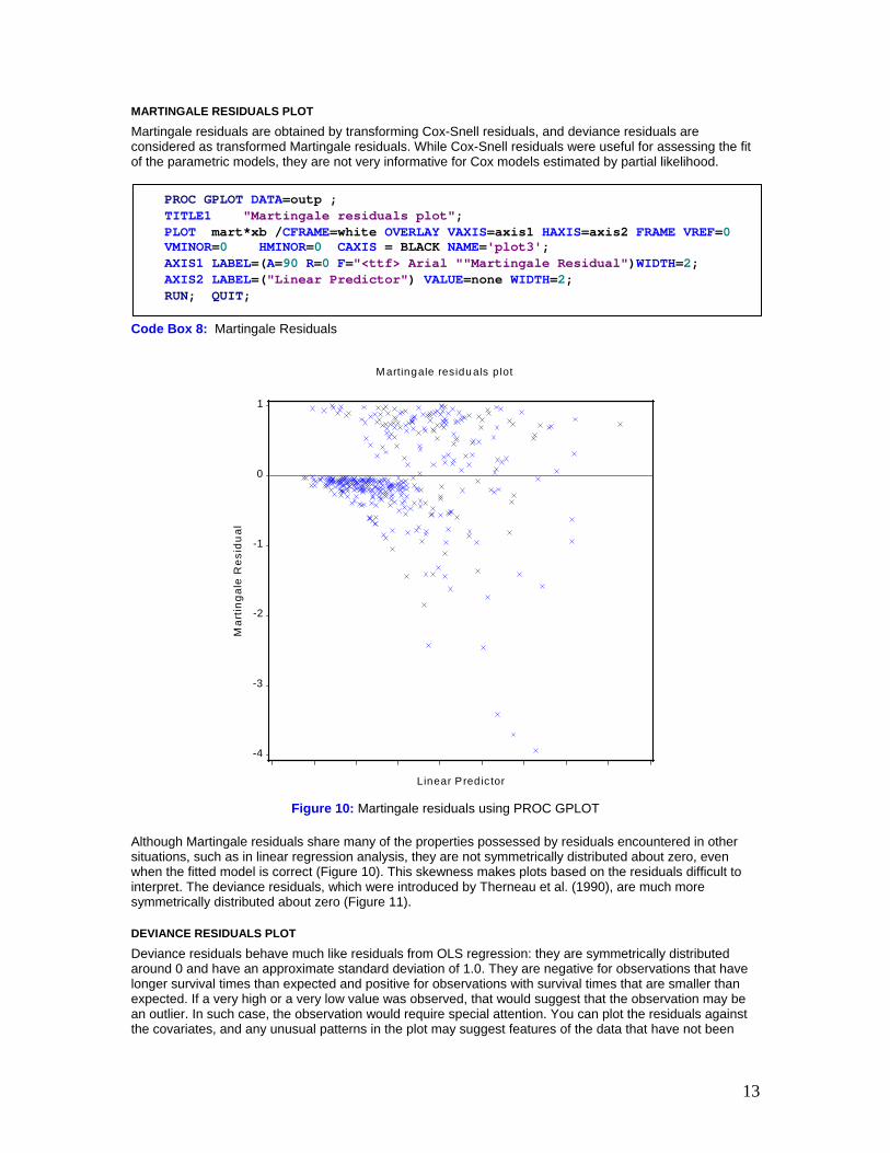
Martingale residuals are obtained by transforming Cox-Snell residuals, and deviance residuals are considered as transformed Martingale residuals. While Cox-Snell residuals were useful for assessing the fit of the parametric models, they are not very informative for Cox models estimated by partial likelihood.

PROC GPLOT DATA=outp ; TITLE1 "Martingale residuals plot"; PLOT mart*xb /CFRAME=white OVERLAY VAXIS=axis1 HAXIS=axis2 FRAME VREF=0 VMINOR=0 HMINOR=0 CAXIS = BLACK NAME='plot3'; AXIS1 LABEL=(A=90 R=0 F="<ttf> Arial ""Martingale Residual")WIDTH=2; AXIS2 LABEL=("Linear Predictor") VALUE=none WIDTH=2; RUN; QUIT;

Code Box 8: Martingale Residuals

M artingale residuals plot

Mar

tinga

le R

esid

ual

-4

-3

-2

-1

0

1

Linear Predic tor

Figure 10: Martingale residuals using PROC GPLOT

Although Martingale residuals share many of the properties possessed by residuals encountered in other situations, such as in linear regression analysis, they are not symmetrically distributed about zero, even when the fitted model is correct (Figure 10). This skewness makes plots based on the residuals difficult to interpret. The deviance residuals, which were introduced by Therneau et al. (1990), are much more symmetrically distributed about zero (Figure 11).

DEVIANCE RESIDUALS PLOT

Deviance residuals behave much like residuals from OLS regression: they are symmetrically distributed around 0 and have an approximate standard deviation of 1.0. They are negative for observations that have longer survival times than expected and positive for observations with survival times that are smaller than expected. If a very high or a very low value was observed, that would suggest that the observation may be an outlier. In such case, the observation would require special attention. You can plot the residuals against the covariates, and any unusual patterns in the plot may suggest features of the data that have not been

13

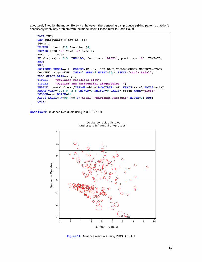
adequately fitted by the model. Be aware, however, that censoring can produce striking patterns that don't necessarily imply any problem with the model itself. Please refer to Code Box 9.

DATA INF; SET outp(where =(dev ne .)); id=_n_; LENGTH text $12 function $8; RETAIN XSYS '2' YSYS '2' size 1; X=xb ; Y=dev; IF abs(dev) > 2.5 THEN DO; function= 'LABEL'; position= '8'; TEXT=ID; END; RUN; GOPTIONS RESET=all COLORS=(Black, RED,BLUE,YELLOW,GREEN,MAGENTA,CYAN) dev=EMF target=EMF XMAX=7 YMAX=7 HTEXT=14pt FTEXT="<ttf> Arial"; PROC GPLOT DATA=outp ; TITLE1 "Deviance residuals plot"; TITLE2 "Outlier and influential diagnostics "; BUBBLE dev*xb=lmax /CFRAME=white ANNOTATE=inf VAXIS=axis1 HAXIS=axis2 FRAME VREF=-2.5 0 2.5 VMINOR=0 HMINOR=0 CAXIS= black NAME='plot3' BCOLOR=red BSIZE=12; AXIS1 LABEL=(A=90 R=0 F="Arial ""Deviance Residual")WIDTH=2; RUN; QUIT;

Code Box 9: Deviance Residuals using PROC GPLOT

87

119

253 293

319

331 393

Dev iance res iduals p lotOu tlier and influential d iagnostics

Dev

ianc

e R

esid

ual

-3

-2

-1

0

1

2

3

4

Linear Predictor

1 2 3 4 5 6 7 8 9 10

Figure 11: Deviance residuals using PROC GPLOT

14

Figure 11 shows deviance residuals with influential data and outliers. As we can see, numbers 87, 119, 292, 319, 331, 253, and 293 are outliers. The diameter of bubble is proportional to LMAX statistic. Observations with relatively large bubbles can be considered as the influential observations. The big bubbles inside the lines are not outliers, but are highly influential.

CONCLUSION In this paper, we demonstrated a comprehensive set of tools and plots to conduct survival analysis and Cox’s proportional hazard functions. We presented key features such as estimated hazard function, survival function, cumulative Martingale residual plots, and outlier detection plots using PROCS LIFEREG, LIFETEST, PHREG, BPHREG and ODS Statistical Graphics. The ODS Statistical Graphics capability enables us to make customized graphics with ease. Furthermore, we showed the solutions to the limitations in the PHREG PROC in producing ODS Graphics in the presence of both STRATA and ASSESS statements in SAS version 9.1.3. By using the experimental BPHREG procedure and the new CLASS statement, we showed how to produce the cumulative residual plots using the ODS Graphics. It is noteworthy that PROC BPHREG is now integrated in PROC PHREG in version 9.2. In conclusion, ODS Statistical Graphics is an extremely useful new feature in SAS that allows the creation of sophisticated statistical graphics. The graphs will maintain a professional appearance, and with the use of styles, will look consistent with other ODS output.

REFERENCES Gharibvand, L. and Fernandez, G. (2008), “Advanced Statistical and Graphical features of SAS® PHREG”, SAS GLOBAL Forum 2008 Conference proceedings San Antonio TX http://www2.sas.com/proceedings/forum2008/375-2008.pdf Gharibvand, L. and Fernandez, G. (2007), “Survival Analysis Plots Using SAS ® ODS Graphics”, Western Users of SAS Software (WUSS) 2007 Conference proceedings San Francisco, CA http://www.crda.unr.edu/crda/publications/ANL_Gharibvand_SurvivalAnalysis.pdf Lin, D. and Wei, L. and Ying, Z. (1993), "Checking the Cox Model with Cumulative Sums of Martingale-Based Residuals", Biometrika, 80, 557 - 572 SAS Institute, Inc. (2005), “TEMPLATE Procedure: Creating ODS Statistical Graphics Output (Experimental)” http://support.sas.com/rnd/base/topics/statgraph/proctemplate/a002774500.htm SAS Institute, Inc. (2007a), SAS/STAT ® User’s Guide, SAS OnlineDoc® 9.1.3, Cary, NC: SAS Institute, Inc. SAS Institute, Inc. (2007b), PHREG: SAS/STAT ® User’s Guide, SAS OnlineDoc® 9.1.3 http://support.sas.com/91doc/getDoc/statug.hlp/phreg_index.htm Cary, NC: SAS Institute, Inc. SAS Institute, Inc. (2007c), BPHREG: SAS/STAT ® User’s Guide, SAS OnlineDoc® 9.1.3 http://support.sas.com/rnd/app/papers/bayesian.pdf Therneau, T.M. and Grambsch, P.M. and Fleming, T.R. (1990), “Martingale-based residuals for survival models”, Biometrika 1990 77(1):147-160 Shtatland, E.S. and Kleinman, K. and Cain, E.M. (2005), “MODEL BUILDING IN PROC PHREG WITH AUTOMATIC VARIABLE SELECTION AND INFORMATION CRITERIA”, online proceedings paper, SAS Users Global Forum 2005 http://www2.sas.com/proceedings/sugi30/206-30.pdf

15

CONTACT INFORMATION Your comments are greatly appreciated and encouraged. Contact the author at: Lida Gharibvand University of California, Riverside Work Phone: (949) 230-5439 Email: lida.gharibvand@email.ucr.edu SAS and all other SAS Institute Inc. product or service names are registered trademarks or trademarks of SAS Institute Inc. in the USA and other countries. ® indicates USA registration. Other brand and product names are trademarks of their respective companies.

16