A standardized boundary element method volume conductor model

Manfred Fuchsa,*, Jorn Kastnera, Michael Wagnera, Susan Hawesb, John S. Ebersoleb

aNeuroscan Laboratories, Lutterothstrasse 28e, D-20255 Hamburg, GermanybUniversity of Chicago, Chicago, IL 60637, USA

Accepted 23 January 2002

Abstract

Objectives: We used a 3-compartment boundary element method (BEM) model from an averaged magnetic resonance image (MRI) data

set (Montreal Neurological Institute) in order to provide simple access to realistically shaped volume conductor models for source recon-

struction, as compared to individually derived models. The electrode positions were transformed into the model’s coordinate system, and the

best fit dipole results were transformed back to the original coordinate system. The localization accuracy of the new approach was tested in a

comparison with simulated data and with individual BEM models of epileptic spike data from several patients.

Methods: The standard BEM model consisted of a total of 4770 nodes, which describe the smoothed cortical envelope, the outside of the

skull, and the outside of the skin. The electrode positions were transformed to the model coordinate system by using 3–5 fiducials (nasion, left

and right preauricular points, vertex, and inion). The transformation consisted of an averaged scaling factor and a rigid transformation

(translation and rotation). The potential values at the transformed electrode positions were calculated by linear interpolation from the stored

transfer matrix of the outer BEM compartment triangle net. After source reconstruction the best fit dipole results were transformed back into

the original coordinate system by applying the inverse of the first transformation matrix.

Results: Test-dipoles at random locations and with random orientations inside of a highly refined reference BEM model were used to

simulate noise-free data. Source reconstruction results using a spherical and the standardized BEM volume conductor model were compared

to the known dipole positions. Spherical head models resulted in mislocation errors at the base of the brain. The standardized BEM model

was applied to averaged and unaveraged epileptic spike data from 7 patients. Source reconstruction results were compared to those achieved

by 3 spherical shell models and individual BEM models derived from the individual MRI data sets. Similar errors to that evident with

simulations were noted with spherical head models. Standardized and individualized BEM models were comparable.

Conclusions: This new approach to head modeling performed significantly better than a simple spherical shell approximation, especially

in basal brain areas, including the temporal lobe. By using a standardized head for the BEM setup, it offered an easier and faster access to

realistically shaped volume conductor models as compared to deriving specific models from individual 3-dimensional MRI data. q 2002

Elsevier Science Ireland Ltd. All rights reserved.

Keywords: Boundary element method; EEG; Triangle refinement; Source reconstruction; Localization accuracy

1. Introduction

The boundary element method (BEM) improves the loca-

lization accuracy of bioelectric source reconstruction results,

as compared to simple spherical shell models, by approximat-

ing the volume conductor properties of realistically shaped

compartments of isotropic and homogeneous conductivities.

The anisotropy and fine structure of the real tissue surround-

ing the electric sources to be reconstructed are purposefully

neglected. These factors can in principle be treated by finite

element methods (FEM), but they suffer from large computa-

tional effort and in vivo conductivity and anisotropy para-

meters that are mostly unknown. The BEM is a compromise

between over-simplified, spherically symmetric models, that

reflect only mean conductivities but not the shape of the

compartments, and overly complex models for which

detailed real tissue data are not available (Geddes and

Baker, 1963; Law, 1993; van Burik and Peters, 2000).

Many authors have already discussed and improved the

BEM (Geselowitz, 1967; Hamalainen and Sarvas, 1989;

Meijs et al., 1989; Oostendorp and van Oosterom, 1989;

Cuffin, 1990; Fletcher et al., 1995; Yvert et al., 1995; Fergu-

son and Stroink, 1997; Fuchs et al., 1998, 2001; Musha and

Okamoto, 1999; Frijns et al., 2000). The BEM requires a

description of the compartment surfaces by closed triangle

meshes with a limited number of nodes. It is limited by the

computational power and the memory requirement for stor-

ing the huge BEM system matrix. The matrix size is propor-

Clinical Neurophysiology 113 (2002) 702–712

1388-2457/02/$ - see front matter q 2002 Elsevier Science Ireland Ltd. All rights reserved.

PII: S1388-2457(02)00030-5

www.elsevier.com/locate/clinph

CLINPH 2001649

* Corresponding author. Tel.: 149-40-4018-9944; fax: 149-40-4018-

9949.

E-mail address: mfuchs@neuroscan.com (M. Fuchs).

tional to the square of the total number of nodes, and the

computational effort to decompose the BEM matrix is

proportional to the third power of the number of nodes,

whereas the accuracy of the BEM is roughly proportional

to the number of nodes representing the realistic model. The

computation time needed for a forward calculation of the

electric potential distribution at the given electrode posi-

tions is also proportional to the number of nodes and to

the number of electrodes.

In this investigation, we developed a standardized BEM

model (sBEM) from averaged magnetic resonance imaging

(MRI) data (Montreal Neurological Institute), having

computed and stored the transfer matrix for all nodes of

the outermost (skin) compartment. The measured electrode

positions were transformed and scaled to the sBEM model

coordinate system, which is aligned by the PreAuricular

points and the Nasion (PAN system). The electric potential

values at the transformed electrode positions were calcu-

lated by linear interpolation from the nodes of the sBEM

model skin compartment. Finally the source reconstruction

results were transformed back to the original electrode coor-

dinate system by applying the inverse transformations.

By doing so we eliminated the need to segment an indi-

vidual subject’s anatomical data into the 3 main BEM model

compartments, which requires sophisticated algorithms or

manual interaction. If overlay of the source reconstruction

results with the individual anatomy is not required, the

subject’s anatomical image data are not at all needed.

Furthermore the time consuming BEM matrix setup and

decomposition steps can be omitted. Thus an easier and

much faster access to realistically shaped volume conductor

models can be achieved.

2. Methods

2.1. The boundary element method

The boundary element method (BEM) allows to calculate

the electric potential V of a current source in an inhomoge-

neous conductor by solving the following integral equation,

if the conducting object is divided by closed surfaces Si

(i ¼ 1;…; nsÞ into ns compartments, each having a different

enclosed isotropic conductivity s inj . The electric potential at

position r [ Sk is then given by (Geselowitz, 1967; Sarvas,

1987):

�s kVðrÞ ¼ s0V0ðrÞ 11

4p

Xns

i¼1

Ds i %Si

Vðr 0Þ nðr 0Þ·r 02 r

r 0 2 rj j3

dSi‘ ð1Þ

with V0 representing the potential of the source in an unlim-

ited homogeneous medium with conductivity s 0, the mean

conductivity �s k ¼ ðs ink 1 s out

k Þ=2, and the conductivity

differences Ds i ¼ s ini 2 s out

i . To calculate the electric

fields it is necessary to approximate numerically the two

integrals over the closed surfaces Si of the conductor bound-

aries consisting of differential surface elements (dS0

i) and

with surface normal orientations n at positions r 0. The

surfaces are described by a large number of small triangles

and the integrals are replaced by summations over these

triangle areas. Different assumptions about the variation of

the potential over the triangle area can be applied (van

Oosterom and Strackee, 1983; de Munck, 1992; Ferguson

et al., 1994; Schlitt et al., 1995; Fuchs et al., 1998): aver-

aged, regionally constant, linear, and quadratic dependen-

cies. The potential values or the coefficients of the basis

functions used to approximate the potentials on the surface

elements form a vector of unknowns, which can be solved

through the following matrix formulation:

�sV ¼ s0V0 1 BV ) V ¼ �s 2 B� �21

s0V0 ð2Þ

If one explicitly solves Eq. (2) just for the fixed number of

measurement positions, a transfer matrix T is obtained, that

relates the sensor signals to the homogeneous potentials

(e.g. Fletcher et al., 1995). The potential vector V , that

contains the field distribution at all skin nodes, generated

by a (dipolar) source inside the innermost compartment

(brain) can thus be easily computed by a simple matrix-

vector multiplication:

V ¼ TV0 with T ¼ �s 2 B� �21

s0 ð3Þ

The column vector V0 contains the electric potential

values V0i of all skin-nodes i at position ri for the source

in an infinite homogeneous conductor with conductivity s0

(dipole at position r j, current j:

V0i ¼1

4ps0

jri 2 rj

ri 2 rj

��� ���3 ð4Þ

2.2. A standardized boundary element method model

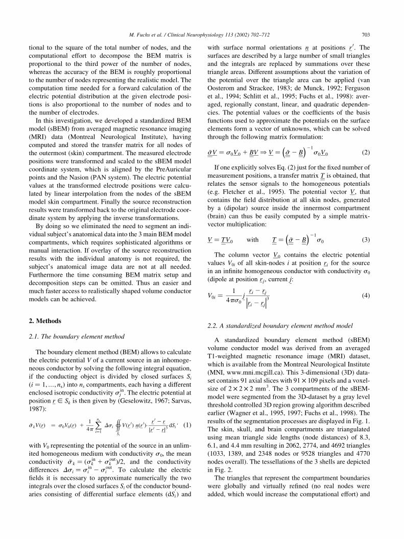
A standardized boundary element method (sBEM)

volume conductor model was derived from an averaged

T1-weighted magnetic resonance image (MRI) dataset,

which is available from the Montreal Neurological Institute

(MNI, www.mni.mcgill.ca). This 3-dimensional (3D) data-

set contains 91 axial slices with 91 £ 109 pixels and a voxel-

size of 2 £ 2 £ 2 mm3. The 3 compartments of the sBEM-

model were segmented from the 3D-dataset by a gray level

threshold controlled 3D region growing algorithm described

earlier (Wagner et al., 1995, 1997; Fuchs et al., 1998). The

results of the segmentation processes are displayed in Fig. 1.

The skin, skull, and brain compartments are triangulated

using mean triangle side lengths (node distances) of 8.3,

6.1, and 4.4 mm resulting in 2062, 2774, and 4692 triangles

(1033, 1389, and 2348 nodes or 9528 triangles and 4770

nodes overall). The tessellations of the 3 shells are depicted

in Fig. 2.

The triangles that represent the compartment boundaries

were globally and virtually refined (no real nodes were

added, which would increase the computational effort) and

M. Fuchs et al. / Clinical Neurophysiology 113 (2002) 702–712 703

a regionally constant potential approximation over the sub-

triangles was chosen. This approach results in better accu-

racy than the standard linear potential approximation (de

Munck, 1992) with comparable computational effort

(Fuchs et al., 1998, 2001). The size of the BEM matrix

stays the same (total number of nodes is unchanged), only

during set up of the system matrix the solid angle computa-

tion is slightly more demanding. In order to further improve

the model accuracy, the isolated problem approach (IPA)

(Hamalainen and Sarvas, 1989) was used.

From the decomposed BEM matrix B the transfer matrix

T for all 1033 nodes of the outermost compartment (skin) is

computed and stored (Eq. (3)).

All these initial computations were performed using the

Curry V4.5 software package (Neuroscan).

2.3. Coordinate system matching

In order to match the coordinate system of the electrodes

and landmarks with the coordinate system of the sBEM

model, both systems were transformed into PAN systems

(PreAuricular points and Nasion). In the PAN system the x-

axis points from the left to the right preauricular point, and

the coordinate system origin is in the middle between both

preauricular points. The y-axis points towards the nasion

(posterior - anterior direction) and lies in the plane of all 3

points. Thus, with asymmetric head shapes the nasion’s x-

coordinate is not always at x ¼ 0. Finally, the z-axis points

from the bottom to the top towards the vertex at right angles

between both x- and y-axes forming a right handed basis.

Details of the coordinate system matching algorithm are

described in Appendix A.

In order to improve the match between the sBEM model

dimensions and the electrodes a global scaling factor was

applied to the electrode positions. It was calculated from

the average of the ratios of the nasion-origin distances and

the left-right preauricular point distances. The inverse of this

factor has to be applied to the reconstruction results before

M. Fuchs et al. / Clinical Neurophysiology 113 (2002) 702–712704

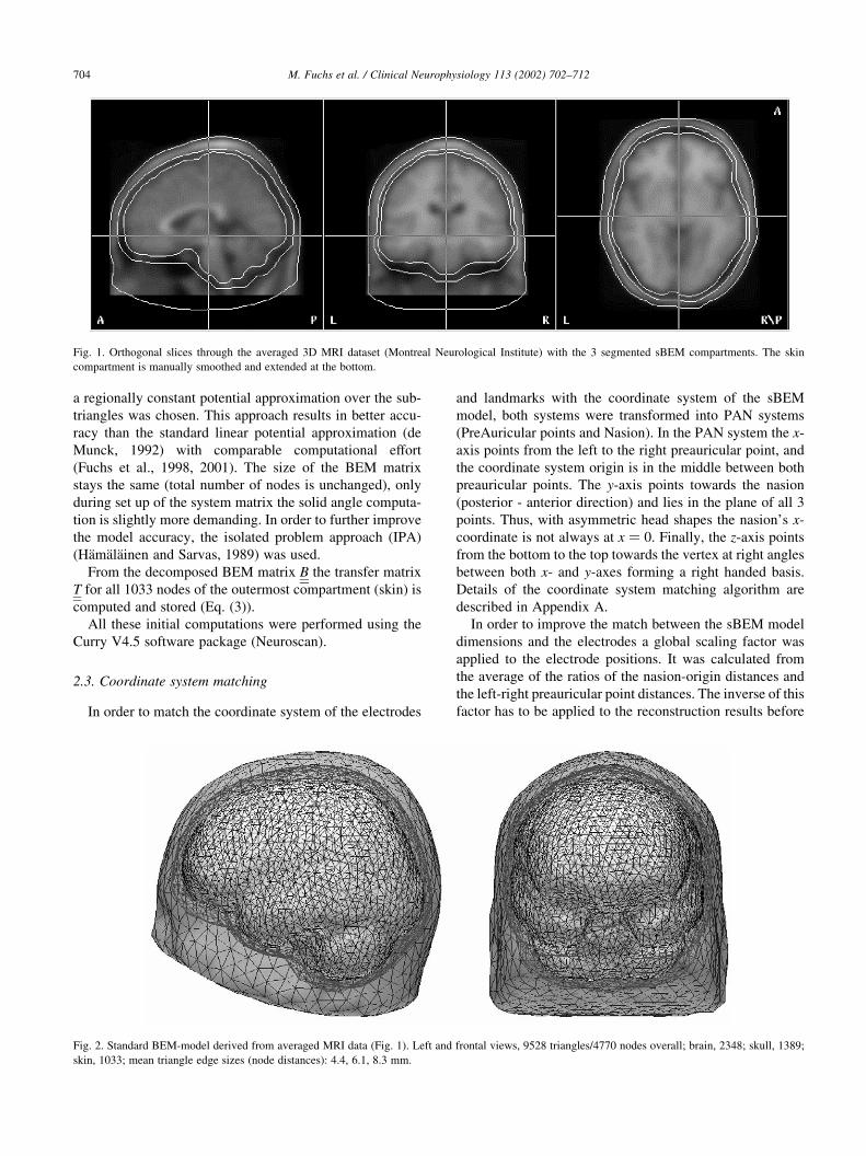
Fig. 2. Standard BEM-model derived from averaged MRI data (Fig. 1). Left and frontal views, 9528 triangles/4770 nodes overall; brain, 2348; skull, 1389;

skin, 1033; mean triangle edge sizes (node distances): 4.4, 6.1, 8.3 mm.

Fig. 1. Orthogonal slices through the averaged 3D MRI dataset (Montreal Neurological Institute) with the 3 segmented sBEM compartments. The skin

compartment is manually smoothed and extended at the bottom.

the transformation to the original coordinate system can be

performed.

2.4. Linear interpolation of the electrode potentials

The transfer matrix Tof the sBEM model (Eq. (3)) was

used to calculate the electric potential values of a dipolar

source inside the innermost (brain) BEM model compart-

ment at all nodes of the outermost (skin) BEM model

compartment. In order to compute the potential values at

the measured and transformed electrode positions their loca-

tions are projected to the nearest triangle of the skin mesh

and a linear interpolation between the 3 potential values of

the corresponding triangle nodes is performed (Fig. 3).

Details of the linear potential interpolation algorithm are

described in Appendix B.

All sBEM model computations are carried out using the

Source V2.0 software module (Neuroscan).

2.5. Simulations

In order to assess the improvements in source localization

accuracy of the sBEM approach as compared to a spherical

shell model, simulations using a highly refined BEM model

derived from an unaveraged 3D-MR dataset were

performed. This reference BEM model consists of 5275

nodes in total (brain/skull/skin compartment: 2720/1350/

1205; mean node distances: 4.0/6.0/7.4 mm; conductivities:

0.33/0.0042/0.33 S/m). Seventy-one electrodes at extended

10–20 system positions were used to compute the electric

field distributions of 4156 randomly oriented test dipoles

placed at randomly chosen locations inside the brain

compartment.

In order to see the systematic effects of different volume

conductor models on dipole localization without random

localization errors produced by measurement noise, dipoles

were fitted using the noise-free simulated data of the refer-

ence model. First, a spherical model was set up by fitting a

sphere to the electrode positions. This sphere represented

the skin compartment, whereas the spherical shells repre-

senting the skull and brain compartments were derived by

applying relative radii of 93 and 85%. The nonlinear dipole

fit procedure (simplex algorithm, Nelder and Mead, 1965)

started at the known test dipole positions. Finally the loca-

lization error E was determined for each dipole (index

j ¼ 1…N) from the 3-dimensional distance of the known

test-position Pj and the fitted dipole position Rj and the

mean error M is calculated:

Ej ¼

ffiffiffiffiffiffiffiffiffiffiffiffiffiffiffiffiffiffiffiffiffiXi¼x;y;z

Rji 2 Pji

� �2s

ð5Þ

M ¼1

N

Xj¼1::N

Ej ð6Þ

The same evaluations were then performed using the

sBEM model (4770 nodes overall) with the electrodes trans-

formed and matched to the sBEM coordinate system as

described above.

The effect of measurement noise to the localization accu-

racy and stability especially in areas close to the compart-

ment boundaries (Fuchs et al., 2001) is beyond the scope of

this work and thus not studied here in more detail.

2.6. Epileptic spike data

For a more realistic comparison of individual BEM, stan-

dardized BEM, and spherical volume conductor models, 11

averaged epileptic spikes from 7 patients and 12 unaveraged

spikes from one such patient were evaluated. Spike poten-

tials that were used for averages were acquired during stan-

dard long-term EEG monitoring using 26–32 scalp

electrodes (International 10–20 plus bilateral supplementary

subtemporal placements (F9, T9, M1, F10, T10, M2) plus

selected 10–10 intermediary positions). Averages in a given

patient were derived from 3 to 8 individual spikes with the

best signal to noise ratio that had the same voltage topogra-

phy over the time course of the spike. Unaveraged spikes

were obtained from one patient during a standard EEG with

21 electrodes.

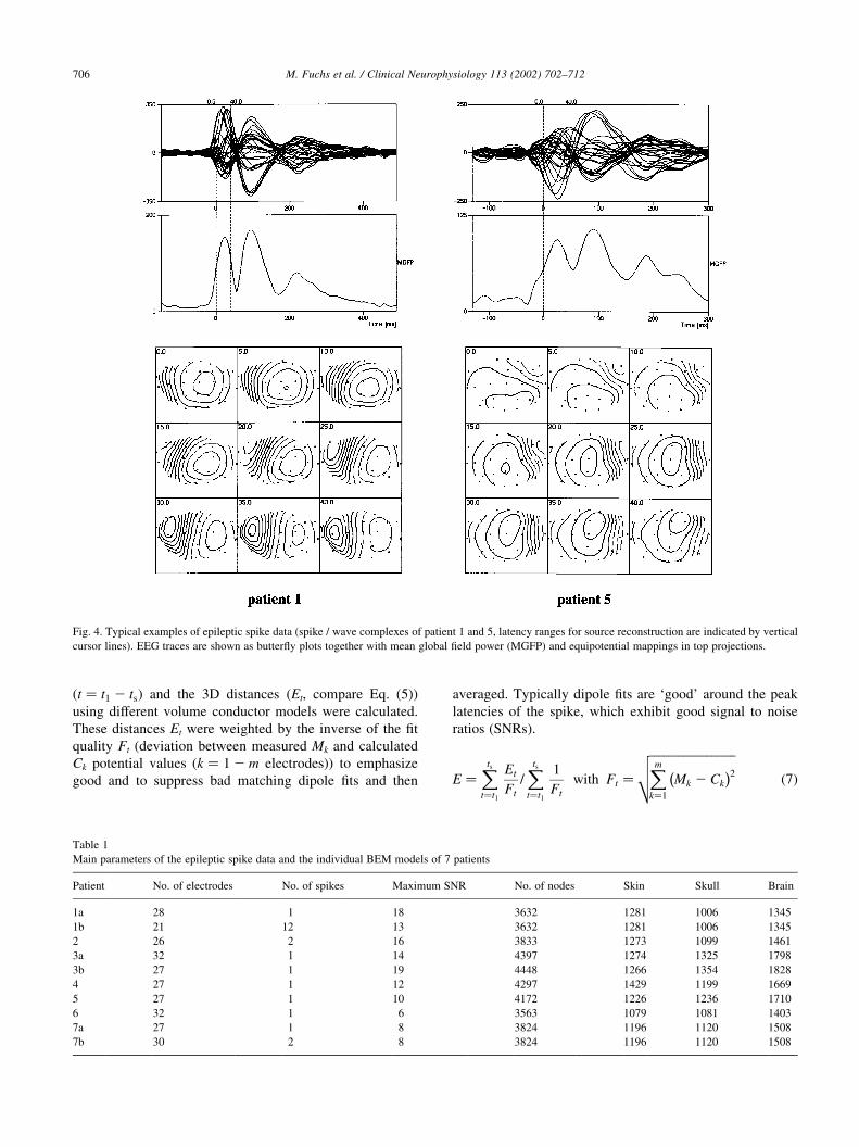
Two typical spike complexes are shown in Fig. 4 as time

courses and as two-dimensional voltage maps. Individual,

realistically shaped BEM compartments (Fig. 5) were

constructed from T1-weighted MR data of the patients by

an automated procedure (Wagner et al., 1995, 1997; Fuchs

et al., 1998). The main parameters of all measurements and

the individual BEM models used can be found in Table 1.

In order to make comparisons, source reconstructions

using standard BEM and spherical shell (outer radius fitted

to the electrodes) models were performed, and the 3D loca-

lization differences between the source models were evalu-

ated. In order to determine mean localization differences

(E), single moving dipoles were fitted at all spike latencies

M. Fuchs et al. / Clinical Neurophysiology 113 (2002) 702–712 705

Fig. 3. Linear interpolation of the electric potential at the projected elec-

trode position Rp. The electrode is projected to the closest triangle, the

weights for the potentials at the triangle nodes are calculated from the ratios

of the sub-triangle areas Aij to the total triangle area.

(t ¼ t1 2 ts) and the 3D distances (Et, compare Eq. (5))

using different volume conductor models were calculated.

These distances Et were weighted by the inverse of the fit

quality Ft (deviation between measured Mk and calculated

Ck potential values (k ¼ 1 2 m electrodes)) to emphasize

good and to suppress bad matching dipole fits and then

averaged. Typically dipole fits are ‘good’ around the peak

latencies of the spike, which exhibit good signal to noise

ratios (SNRs).

E ¼Xtst¼t1

Et

Ft

=Xts

t¼t1

1

Ft

with Ft ¼

ffiffiffiffiffiffiffiffiffiffiffiffiffiffiffiffiffiffiXmk¼1

Mk 2 Ck

� �2vuut ð7Þ

M. Fuchs et al. / Clinical Neurophysiology 113 (2002) 702–712706

Fig. 4. Typical examples of epileptic spike data (spike / wave complexes of patient 1 and 5, latency ranges for source reconstruction are indicated by vertical

cursor lines). EEG traces are shown as butterfly plots together with mean global field power (MGFP) and equipotential mappings in top projections.

Table 1

Main parameters of the epileptic spike data and the individual BEM models of 7 patients

Patient No. of electrodes No. of spikes Maximum SNR No. of nodes Skin Skull Brain

1a 28 1 18 3632 1281 1006 1345

1b 21 12 13 3632 1281 1006 1345

2 26 2 16 3833 1273 1099 1461

3a 32 1 14 4397 1274 1325 1798

3b 27 1 19 4448 1266 1354 1828

4 27 1 12 4297 1429 1199 1669

5 27 1 10 4172 1226 1236 1710

6 32 1 6 3563 1079 1081 1403

7a 27 1 8 3824 1196 1120 1508

7b 30 2 8 3824 1196 1120 1508

3. Results

3.1. Simulations

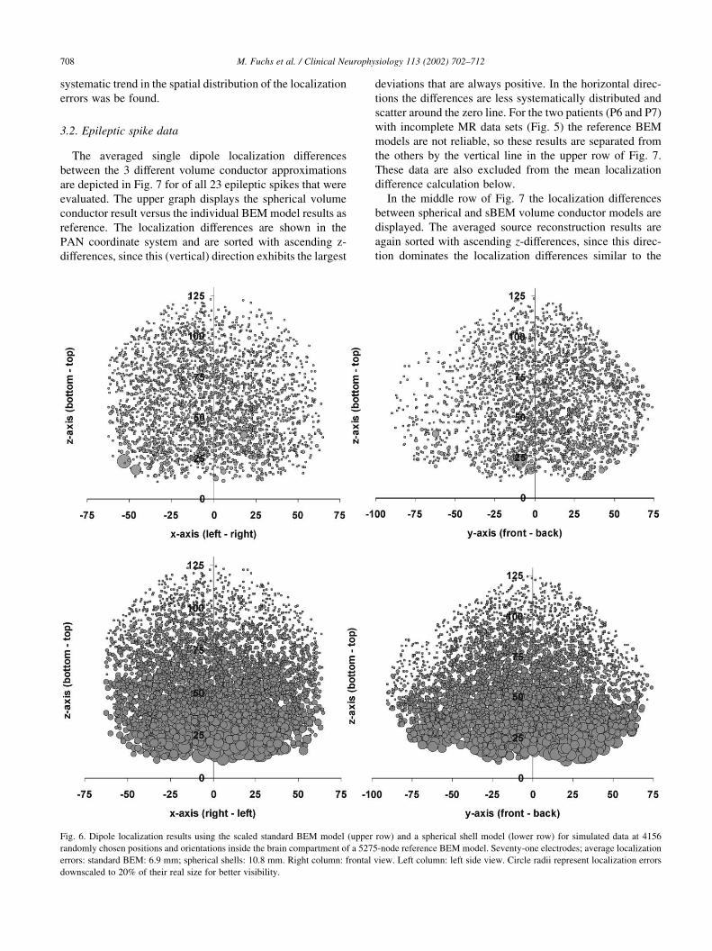
The spatial distributions of the localization errors for both

sBEM and spherical volume conductor models using simu-

lated data are displayed in Fig. 6. The localization errors are

represented by the radii of circles centered at the true posi-

tions of the test-dipoles with the reference BEM model. For

better visibility the radii are downscaled by a factor of 5 to

20% of their real size. The mean location errors averaged

over all 4156 randomly distributed test-dipole positions are

6.9 mm for the sBEM model and 10.8 mm for the 3 spherical

shells model. More important than the improvement in the

absolute localization accuracy is the more homogeneous

spatial distribution of the localization errors with the

sBEM model. The spherical model performs best in the

more spherical upper parts of the brain, but fails in the

lower frontal, central, and temporal lobe areas, which

cannot be well represented by the spherical shells. These

findings confirm the earlier studies that showed the same

behavior (Fuchs et al., 1998, 2001). For the sBEM model no

M. Fuchs et al. / Clinical Neurophysiology 113 (2002) 702–712 707

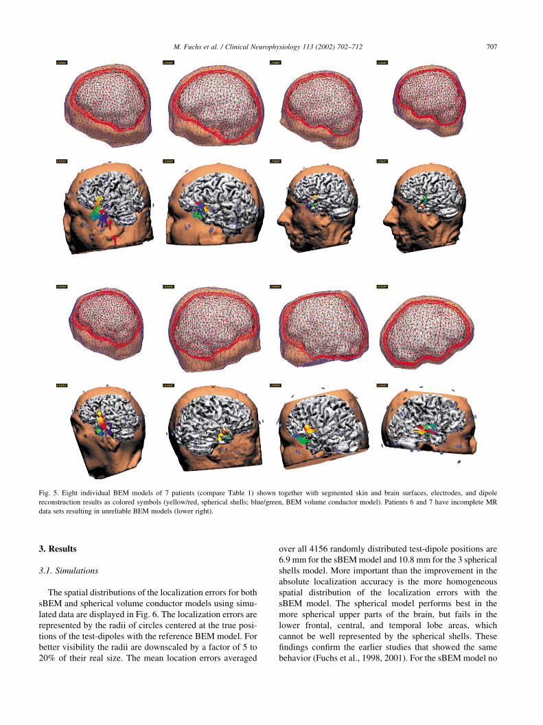
Fig. 5. Eight individual BEM models of 7 patients (compare Table 1) shown together with segmented skin and brain surfaces, electrodes, and dipole

reconstruction results as colored symbols (yellow/red, spherical shells; blue/green, BEM volume conductor model). Patients 6 and 7 have incomplete MR

data sets resulting in unreliable BEM models (lower right).

systematic trend in the spatial distribution of the localization

errors was be found.

3.2. Epileptic spike data

The averaged single dipole localization differences

between the 3 different volume conductor approximations

are depicted in Fig. 7 for of all 23 epileptic spikes that were

evaluated. The upper graph displays the spherical volume

conductor result versus the individual BEM model results as

reference. The localization differences are shown in the

PAN coordinate system and are sorted with ascending z-

differences, since this (vertical) direction exhibits the largest

deviations that are always positive. In the horizontal direc-

tions the differences are less systematically distributed and

scatter around the zero line. For the two patients (P6 and P7)

with incomplete MR data sets (Fig. 5) the reference BEM

models are not reliable, so these results are separated from

the others by the vertical line in the upper row of Fig. 7.

These data are also excluded from the mean localization

difference calculation below.

In the middle row of Fig. 7 the localization differences

between spherical and sBEM volume conductor models are

displayed. The averaged source reconstruction results are

again sorted with ascending z-differences, since this direc-

tion dominates the localization differences similar to the

M. Fuchs et al. / Clinical Neurophysiology 113 (2002) 702–712708

Fig. 6. Dipole localization results using the scaled standard BEM model (upper row) and a spherical shell model (lower row) for simulated data at 4156

randomly chosen positions and orientations inside the brain compartment of a 5275-node reference BEM model. Seventy-one electrodes; average localization

errors: standard BEM: 6.9 mm; spherical shells: 10.8 mm. Right column: frontal view. Left column: left side view. Circle radii represent localization errors

downscaled to 20% of their real size for better visibility.

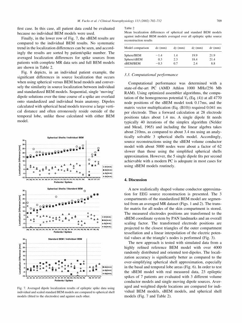
first case. In this case, all patient data could be evaluated

because no individual BEM models were used.

Finally, in the lower row of Fig. 7, the sBEM results are

compared to the individual BEM results. No systematic

trend in the localization differences can be seen, and accord-

ingly the results are sorted by patient/spike number. The

averaged localization differences for spike sources from

patients with complete MR data sets and full BEM models

are shown in Table 2.

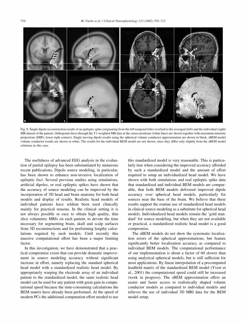
Fig. 8 depicts, in an individual patient example, the

significant differences in source localization that occurs

when using spherical versus BEM head models and conver-

sely the similarity in source localization between individual

and standardized BEM models. Sequential, single ‘moving’

dipole solutions over the time course of a spike are overlaid

onto standardized and individual brain anatomy. Dipoles

calculated with spherical head models traverse a large verti-

cal distance and often erroneously reside outside of the

temporal lobe, unlike those calculated with either BEM

model.

3.3. Computational performance

Computational performance was determined with a

state-of-the-art PC (AMD Athlon 1000 MHz/256 Mb

RAM). Using optimized assembler algorithms, the compu-

tation of the homogeneous potential V0 (Eq. (4)) at all 4770

node positions of the sBEM model took 0.17ms, and the

matrix vector multiplication (Eq. (B10)) required 0.041 ms

per electrode. Thus a forward calculation at 28 electrode

positions takes about 1.4 ms. A single dipole fit needs

typically 40 iterations of the simplex algorithm (Nelder

and Mead, 1965) and including the linear algebra takes

about 210ms, as compared to about 3.4 ms using an analy-

tically solvable 3 spherical shells model. Accordingly,

source reconstructions using the sBEM volume conductor

model with about 5000 nodes were about a factor of 62

slower than those using the simplified spherical shells

approximation. However, the 5 single dipole fits per second

achievable with a modern PC is adequate in most cases for

using sBEM models routinely.

4. Discussion

A new realistically shaped volume conductor approxima-

tion for EEG source reconstruction is presented. The 3

compartments of the standardized BEM model are segmen-

ted from an averaged MR dataset (Figs. 1 and 2). The trans-

fer matrix for all nodes of the skin compartment is stored.

The measured electrodes positions are transformed to the

sBEM coordinate system by PAN landmarks and an overall

scaling factor. The transformed electrode positions are

projected to the closest triangles of the outer compartment

tessellation and a linear interpolation of the electric poten-

tial values at the triangle’s nodes is performed (Fig. 3).

The new approach is tested with simulated data from a

highly refined reference BEM model with over 4000

randomly distributed and oriented test-dipoles. The locali-

zation accuracy is significantly better as compared to the

over-simplifying spherical shell approximation, especially

in the basal and temporal lobe areas (Fig. 6). In order to test

the sBEM model with real measured data, 23 epileptic

spikes of 7 patients are evaluated with 3 different volume

conductor models and single moving dipole sources. Aver-

aged and weighted dipole locations are compared for indi-

vidual BEM models, sBEM models, and spherical shell

models (Fig. 7 and Table 2).

M. Fuchs et al. / Clinical Neurophysiology 113 (2002) 702–712 709

Fig. 7. Averaged dipole localization results of epileptic spike data using

individual and scaled standard BEM models are compared to spherical shell

models (fitted to the electrodes) and against each other.

Table 2

Mean localization differences of spherical and standard BEM models

against individual BEM models averaged over all epileptic spike source

reconstruction results

Model comparison dx (mm) dy (mm) dz (mm) dr (mm)

Sphere/BEM 21.4 1.4 19.9 21.9

Sphere/sBEM 0.3 2.3 18.4 21.4

sBEM/BEM 20.3 0.7 2.4 8.8

The usefulness of advanced EEG analysis in the evalua-

tion of partial epilepsy has been substantiated by numerous

recent publications. Dipole source modeling, in particular,

has been shown to enhance non-invasive localization of

epileptic foci. Several previous studies using simulations,

artificial dipoles, or real epileptic spikes have shown that

the accuracy of source modeling can be improved by the

incorporation of 3D head and brain anatomy for both head

models and display of results. Realistic head models of

individual patients have seldom been used clinically

mainly for practical reasons. In the clinical setting it is

not always possible or easy to obtain high quality, thin

slice volumetric MRIs on each patient, to devote the time

necessary for segmenting brain, skull and scalp surfaces

from 3D reconstructions and for performing lengthy calcu-

lations required by such models. Until recently this

massive computational effort has been a major limiting

factor.

In this investigation, we have demonstrated that a prac-

tical compromise exists that can provide dramatic improve-

ment in source modeling accuracy without significant

increase in effort, namely replacing the standard spherical

head model with a standardized realistic head model. By

appropriately warping the electrode array of an individual

patient to the standardized model, the same realistic head

model can be used for any patient with great gain in compu-

tational speed because the time-consuming calculations the

BEM matrix have already been performed. At the speed of

modern PCs the additional computation effort needed to use

this standardized model is very reasonable. This is particu-

larly true when considering the improved accuracy afforded

by such a standardized model and the amount of effort

required to setup an individualized head model. We have

shown with both simulations and real epileptic spike data

that standardized and individual BEM models are compar-

able, that both BEM models delivered improved dipole

accuracy over spherical head models, particularly for

sources near the base of the brain. We believe that these

results support the routine use of standardized head models

in clinical source modeling as a substitute for spherical head

models. Individualized head models remain the ‘gold stan-

dard’ for source modeling, but when they are not available

or practical, a standardized realistic head model is a good

compromise.

The sBEM models do not show the systematic localiza-

tion errors of the spherical approximations, but feature

significantly better localization accuracy as compared to

individual BEM models. The computational performance

of our implementation is about a factor of 60 slower than

using analytical spherical models, but is still sufficient for

most applications. By linear interpolation of a precomputed

leadfield matrix of the standardized BEM model (Yvert et

al., 2001) the computational speed could still be increased

(work in progress). The sBEM approximation offers an

easier and faster access to realistically shaped volume

conductor models as compared to individual models and

relieves the use of individual 3D MRI data for the BEM

model setup.

M. Fuchs et al. / Clinical Neurophysiology 113 (2002) 702–712710

Fig. 8. Single dipole reconstruction results of an epileptic spike (originating from the left temporal lobe) overlaid to the averaged (left) and the individual (right)

MR dataset of the patient. Orthogonal slices through the T1-weighted MR data at the cursor positions (white lines) are shown together with maximum intensity

projections (MIPs, lower right corners). Single moving dipole results using the spherical volume conductor approximation are shown in black, sBEM model

volume conductor results are shown in white. The results for the individual BEM model are not shown, since they differ only slightly from the sBEM model

solutions in this case.

Appendix A. Coordinate system matching

The shift vector S and the rotation matrix M, that are

needed to transform points (e.g. the electrode positions)

from their original coordinate system to their PAN repre-

sentation, can easily be achieved from their original land-

mark coordinates Lo, Ro and No (left and right preauricular

point and nasion). The shift vector S to the PAN origin, that

has to be applied first, is simply the center between both

preauricular points:

S ¼ ðRo 1 LoÞ0:5 ðA1Þ

The x-axis direction in the original coordinate system is:

Xo ¼ ðRo 2 LoÞ= ðRo 2 LoÞj j

with

ðRo 2 LoÞj j ¼ ðRo 2 LoÞðRo 2 LoÞ� �1=2

ðA2Þ

The y-axis is perpendicular to the x-axis and points towards

the nasion, so it can be calculated from the normal compo-

nent of the connection from the PAN origin to the nasion:

Yo ¼ U= Uj j

with

U ¼ ðNo 2 SÞ2 ðNo 2 SÞXo

� �Xo ðA3Þ

The z-axis is finally calculated from the cross-product of the

x- and y-axes:

Zo ¼ Xo £ Yo ðA4Þ

Combining the 3 basis vectors (as column vectors) to a

matrix A results in a rotation matrix that transforms points

from the PAN to the shifted original coordinate system. The

rotation matrix M that converts points from the shifted origi-

nal to the PAN system is simply the inverse of this matrix A:

A ¼ ½XoYoZo� M ¼ A21 ¼ AT ðA5Þ

So finally the combined transformation to transform a point

Po from the original to the PAN coordinate system reads:

Pp ¼ MðPo 2 SÞ ðA6Þ

The inverse transformation is:

Po ¼ M21Pp 1 S ¼ APp 1 S ðA7Þ

Appendix B. Linear interpolation of the electrodepotentials

Let Ri (i ¼ 1…3) be the node positions of the skin triangle

net, then the center position Rc of this triangle is given by

(Fig. 3):

Rc ¼ ðR1 1 R2 1 R3Þ=3 ðB1Þ

For an electrode at position Re the triangle (index n) with the

smallest distance��Re 2 Rcn

�� is searched. The edge vectors of

the closest triangle are calculated:

E12 ¼ R2 2 R1 E23 ¼ R3 2 R2 E31 ¼ R1 2 R3 ðB2Þ

Finally the electrode position is projected to the triangles

area by using the triangle normal N:

N ¼ E12 £ E31 ðB3Þ

The projected position Rp is:

Rp ¼ Re 1 N ðRe 2 RcN� �

=NN ðB4Þ

The weights wi (i ¼ 1::3) for the potential values Vi at the

triangle nodes are computed by linear interpolation from the

projected electrode position. The projected electrode posi-

tion splits the triangle into 3 sub-triangles, their areas Aij are

proportional to the cross products of the connecting lines

from the projected electrode position to the triangle nodes

Cpi and the triangle edges Eij. The total area of the triangle A

is proportional to the sum of the areas of the 3 sub-triangles

Aij:

Cpi ¼ Ri 2 Rp ðB5Þ

Aija Cpi £ Eij

��� ��� AaSAij ðB6Þ

The weighting factors wi are given by the ratios of the

corresponding sub-triangle areas to the total area of the

triangle:

w1 ¼ A23=A w2 ¼ A31=A w3 ¼ A12=A ðB7Þ

So finally the interpolated potential Ve at the (projected)

electrode position is given by the weighted sum of the

node potentials Vi:

Ve ¼ SwiVi ðB8Þ

Since the electric potential Vi at a node i is computed from a

multiplication of the corresponding row Ti of the transfer

matrix T (Eq. (3)) with the homogeneous potential column

vector V0, a new compressed transfer matrix for the

projected electrode positions can be set up:

Te ¼ SwiTi ðB9Þ

With the much smaller transfer matrix Te consisting of rows

Tek for all electrodes k, the forward calculation of the poten-

tials at all electrode positions (column vector Ve) simplifies

to:

Ve ¼ TeV0 with V0 from Eq: ð4Þ: ðB10Þ

References

van Burik MJ, Peters MJ. Estimation of the electric conductivity from scalp

measurements: feasibility and application to source localization. Clin

Neurophysiol 2000;111:1514–1521.

Cuffin BN. Effects of head shape on EEGs and MEGs. IEEE Trans Biomed

Eng 1990;37:44–52.

Ferguson AS, Zhang X, Stroink G. A complete linear discretization for

M. Fuchs et al. / Clinical Neurophysiology 113 (2002) 702–712 711

calculating the magnetic field using the boundary element method.

IEEE Trans Biomed Eng 1994;41:455–460.

Ferguson AS, Stroink G. Factors affecting the accuracy of the boundary

element method in the forward problem I: calculating surface poten-

tials. IEEE Trans Biomed Eng 1997;44:1139–1155.

Fletcher DJ, Amir A, Jewett DL, Fein G. Improved method for computation

of potentials in a realistic head shape model. IEEE Trans Biomed Eng

1995;42:1094–1104.

Frijns JH, de Snoo SL, Schoonhoven R. Improving the accuracy of the

boundary element method by the use of second-order interpolation

functions. IEEE Trans Biomed Eng 2000;47:1336–1346.

Fuchs M, Drenckhahn R, Wischmann HA, Wagner M. An improved bound-

ary element method for realistic volume-conductor modeling. IEEE

Trans Biomed Eng 1998;45:980–997.

Fuchs M, Wagner M, Kastner J. Boundary element method volume conduc-

tor models for EEG source reconstruction. Clin. Neurophysiology

2001;112:1400–1407.

Geddes LA, Baker LE. The specific resistance of biological material, a

compendium of data for the biomedical engineer and physiologist.

Med Biol Eng 1963;5:271–293.

Geselowitz DB. On bioelectric potentials in an inhomogeneous volume

conductor. Biophys J 1967;7:1–17.

Hamalainen MS, Sarvas J. Realistic conductivity geometry model of the

human head for interpretation of neuromagnetic data. IEEE Trans

Biomed Eng 1989;36:165–171.

Law SK. Thickness and resistivity variations over the upper surface of the

human skull. Brain Topogr 1993;6:99–109.

Meijs JWH, Weier OW, Peters MJ, van Oosterom A. On the numerical

accuracy of the boundary element method. IEEE Trans Biomed Eng

1989;36:1038–1049.

de Munck JC. A linear discretization of the volume conductor boundary

integral equation using analytically integrated elements. IEEE Trans

Biomed Eng 1992;39:986–990.

Musha T, Okamoto Y. Forward and inverse problems of EEG dipole loca-

lization. Crit Rev Biomed Eng 1999;27:189–239.

Nelder JA, Mead R. A simplex method for function minimization. Comput

J 1965;7:308–313.

Oostendorp TF, van Oosterom A. Source parameter estimation in inhomo-

geneous volume conductors of arbitrary shape. IEEE Trans Biomed Eng

1989;36:382–391.

van Oosterom A, Strackee J. The solid angle of a plane triangle. IEEE Trans

Biomed Eng 1983;30:125–126.

Sarvas J. Basic mathematical and electromagnetic concepts of the biomag-

netic inverse problem. Phys Med Biol 1987;32:11–22.

Schlitt HA, Heller L, Aaron R, Best E, Ranken DM. Evaluation of boundary

element methods for the EEG forward problem: effect of linear inter-

polation. IEEE Trans Biomed Eng 1995;42:52–58.

Wagner M, Fuchs M, Wischmann HA, Ottenberg K, Dossel O. Cortex

segmentation from 3D MR images for MEG reconstructions. In: Baum-

gartner C, Deecke L, Stroink G, Williamson SJ, editors. Biomagnetism:

fundamental research and clinical applications, Amsterdam: Elsevier

Science/IOS Press, 1995. pp. 352–356.

Wagner M, Fuchs M, Drenckhahn R, Wischmann HA, Kohler T, Theissen

A. Automatic generation of BEM and FEM meshes. Neuroimage

1997;5:389.

Yvert B, Bertrand O, Echallier JF, Pernier J. Improved dipole localization

using local mesh refinement of realistic head geometries. Electroenceph

clin Neurophysiol 1995;95:381–392.

Yvert B, Crouzeix-Cheylus A, Jacques Pernier J. Fast realistic modeling in

bioelectro-magnetism using lead-field interpolation. Hum Brain Mapp

2001;14:48–63.

M. Fuchs et al. / Clinical Neurophysiology 113 (2002) 702–712712