a spreadsheet process model for analysis of costs and life ...jwlevis/dst_collection.pdf · costs...
TRANSCRIPT

A SPREADSHEET PROCESS MODEL
FOR ANALYSIS OF
COSTS AND LIFE-CYCLE INVENTORY PARAMETERS
ASSOCIATED WITH COLLECTION OF
MUNICIPAL SOLID WASTE
Prepared by: Edward M. Curtis, III
and
Robert D. Dumas
North Carolina State University
Prepared for: Dr. Morton A. Barlaz
Department of Civil Engineering
August 7, 2000
i
TABLE OF CONTENTS
1. INTRODUCTION............................................................................................................................1
2. METHODOLOGY...........................................................................................................................6
2.1 COLLECTION SECTORS ........................................................................................................................92.2 COLLECTION “NEXT NODE”..............................................................................................................10
3. COLLECTION COST EQUATIONS ..........................................................................................11
3.1 COST ESCALATION ............................................................................................................................133.2 RESIDENTIAL WASTE COLLECTION ...................................................................................................14
3.2.1 Mixed Waste (C1) ..................................................................................................................153.2.1.1 Generation Rate ........................................................................................................................ 153.2.1.2 Waste Density ........................................................................................................................... 153.2.1.3 Cost Equations .......................................................................................................................... 16
3.2.2 Recyclables (C2, C3, and C4)................................................................................................233.2.2.1 Generation Rate ........................................................................................................................ 233.2.2.2 Waste Density ........................................................................................................................... 253.2.2.3 Cost Equations .......................................................................................................................... 26
3.2.3 Yard Waste (C0 and C9)........................................................................................................313.2.3.1 Generation Rate ........................................................................................................................ 313.2.3.2 Waste Density ........................................................................................................................... 323.2.3.3 Cost Equations .......................................................................................................................... 33
3.2.4 Residuals (C7) .......................................................................................................................363.2.4.1 Generation Rate ........................................................................................................................ 363.2.4.2 Waste Density ........................................................................................................................... 363.2.4.3 Cost Equations .......................................................................................................................... 38
3.2.5 Co-Collection.........................................................................................................................393.2.5.1 Co-Collection Using a Single Compartment Vehicle (C5) .................................................. 393.2.5.2 Co-Collection Using a Two Compartment Vehicle (C6) ...................................................... 39
3.2.5.2.1 Generation Rates ....................................................................................................................... 393.2.5.2.2 Waste Densities ......................................................................................................................... 403.2.5.2.3 Waste Volume ........................................................................................................................... 423.2.5.2.4 Cost Equations........................................................................................................................... 42
3.2.6 Wet/Dry Collection ................................................................................................................433.2.6.1 Wet/Dry/Recyclables (C11) ..................................................................................................... 43
3.2.6.1.1 Dry Waste Generation Rate ....................................................................................................... 443.2.6.1.2 Wet Waste Generation Rate....................................................................................................... 453.2.6.1.3 Recyclables Generation Rate ..................................................................................................... 453.2.6.1.4 Waste Densities ......................................................................................................................... 463.2.6.1.5 Waste Volume ........................................................................................................................... 473.2.6.1.6 Cost Equations........................................................................................................................... 47
3.2.6.2 Wet/Dry (C12) ........................................................................................................................... 483.2.6.2.1 Dry Waste Generation Rate ....................................................................................................... 483.2.6.2.2 Wet Waste Generation Rate....................................................................................................... 493.2.6.2.3 Wet Waste Density .................................................................................................................... 503.2.6.2.4 Dry Waste Density..................................................................................................................... 513.2.6.2.5 Waste Volume ........................................................................................................................... 523.2.6.2.6 Cost Equations........................................................................................................................... 52
3.3 RESIDENTIAL WASTE DROP-OFF.......................................................................................................533.3.1 Recyclables (C8)....................................................................................................................54
3.3.1.1 Generation Rate ........................................................................................................................ 543.3.1.2 Density........................................................................................................................................ 55

ii
3.3.1.3 Cost Equations .......................................................................................................................... 563.3.2 Yard Waste (C10) ..................................................................................................................60
3.3.2.1 Generation Rate ........................................................................................................................ 603.3.2.2 Density........................................................................................................................................ 61
3.4 MULTI-FAMILY DWELLING WASTE COLLECTION ..............................................................................623.4.1 Mixed Waste (C13) ................................................................................................................63
3.4.1.1 Generation Rate ........................................................................................................................ 633.4.1.2 Waste Density ........................................................................................................................... 633.4.1.3 Cost Equations .......................................................................................................................... 64
3.4.2 Recyclables (C14 and C15) ...................................................................................................683.4.2.1 Generation Rate ........................................................................................................................ 683.4.2.2 Waste Density ........................................................................................................................... 703.4.2.3 Cost Equations .......................................................................................................................... 71
3.4.3 Residuals (C16) .....................................................................................................................753.4.3.1 Generation Rate ........................................................................................................................ 753.4.3.2 Waste Density ........................................................................................................................... 753.4.3.3 Cost Equations .......................................................................................................................... 76
3.4.4 Wet/Dry Collection ................................................................................................................783.4.4.1 Wet/Dry/Recyclables (C17) ..................................................................................................... 78
3.4.4.1.1 Dry Waste Generation Rate ....................................................................................................... 793.4.4.1.2 Wet Waste Generation Rate....................................................................................................... 803.4.4.1.3 Recyclables Generation Rate ..................................................................................................... 803.4.4.1.4 Waste Densities ......................................................................................................................... 813.4.4.1.5 Waste Volumes.......................................................................................................................... 823.4.4.1.6 Cost Equations........................................................................................................................... 83
3.4.4.2 Wet/Dry (C18) ........................................................................................................................... 833.4.4.2.1 Dry Waste Generation Rate ....................................................................................................... 833.4.4.2.2 Wet Waste Generation Rate....................................................................................................... 843.4.4.2.3 Wet Waste Density .................................................................................................................... 853.4.4.2.4 Dry Waste Density..................................................................................................................... 863.4.4.2.5 Waste Volume ........................................................................................................................... 873.4.4.2.6 Cost Equations........................................................................................................................... 87
3.5 COMMERCIAL WASTE COLLECTION ..................................................................................................883.5.1 Recyclables (C19)..................................................................................................................90
3.5.1.1 Generation Rate ........................................................................................................................ 903.5.1.2 Waste Density ........................................................................................................................... 913.5.1.3 Cost Equations .......................................................................................................................... 92
3.5.2 Mixed Waste (C20) ................................................................................................................963.5.2.1 Waste Generation Rate ........................................................................................................... 963.5.2.2 Waste Density ........................................................................................................................... 963.5.2.3 Cost Equations .......................................................................................................................... 97
4. COLLECTION VEHICLE CALCULATION PARAMETERS ................................................98
4.1 DAILY ACTIVITY DURATIONS............................................................................................................994.1.1 Residential Curbside, Multi-Family, and Commercial Waste Collection............................1004.1.2 Recyclables Drop-Off ..........................................................................................................103
4.2 DAILY SERVICE HOURS...................................................................................................................1044.2.1 Residential Curbside, Multi-Family, and Commercial Waste Collection............................1054.2.2 Recyclables Drop-Off ..........................................................................................................106
4.3 DAILY MILES TRAVELED ................................................................................................................1074.3.1 Residential Curbside, Multi-Family, and Commercial Waste Collection............................1084.3.2 Recyclables Drop-Off ..........................................................................................................110
4.4 DAILY FUEL USAGE ........................................................................................................................1114.4.1 Residential Curbside, Multi-Family, and Commercial Waste Collection............................1124.4.2 Recyclables Drop-Off ..........................................................................................................114
iii
4.5 DAILY WASTE COLLECTION RATE ..................................................................................................115
5. ENERGY CONSUMPTION EQUATIONS...............................................................................116
5.1 COLLECTION VEHICLES...................................................................................................................1185.2 DROP-OFF VEHICLES ......................................................................................................................119
5.2.1 Recyclables (C8)..................................................................................................................1205.2.2 Yard Waste (C10) ................................................................................................................122
5.3 GARAGE..........................................................................................................................................124
6. WATER CONSUMPTION EQUATIONS.................................................................................126
6.1 COLLECTION VEHICLES...................................................................................................................1276.2 GARAGE..........................................................................................................................................128
7. AIRBORNE RELEASE EQUATIONS......................................................................................129
7.1 COLLECTION VEHICLES...................................................................................................................1317.2 DROP-OFF VEHICLES ......................................................................................................................1327.3 GARAGE..........................................................................................................................................1347.4 GREENHOUSE GAS EQUIVALENCE ..................................................................................................135
8. WATERBORNE RELEASE EQUATIONS ..............................................................................136
8.1 COLLECTION VEHICLES...................................................................................................................1388.2 DROP-OFF VEHICLES ......................................................................................................................1398.3 GARAGE..........................................................................................................................................140
9. SOLID WASTE GENERATION EQUATIONS .......................................................................141
9.1 COLLECTION VEHICLES...................................................................................................................1439.2 DROP-OFF VEHICLES ......................................................................................................................1449.3 GARAGE..........................................................................................................................................145
10. REFERENCES.............................................................................................................................146
APPENDICES............................................................................................................................................147
APPENDIX A – DEFAULT INPUT VALUES (FOR VARIABLES WITHOUT SECTOR OR NEXT NODE
VARIABILITY)..................................................................................................................................148APPENDIX B – DEFAULT INPUT VALUES (FOR VARIABLES WITH SECTOR VARIABILITY)........................182APPENDIX C – DEFAULT INPUT VALUES (FOR VARIABLES WITH SECTOR AND NEXT NODE
VARIABILITY)..................................................................................................................................188APPENDIX D – SAMPLE OUTPUT ..............................................................................................................193APPENDIX E – COEFFICIENTS FOR OPTIMIZATION ....................................................................................242APPENDIX F – VARIABLE NAMES .............................................................................................................255APPENDIX G – COST ESCALATION DATA..................................................................................................267
INTRODUCTION
1
1. INTRODUCTION
A city or county has several options available when it comes to each step in the collectionand disposal of solid waste. These range from simply collecting all municipal solid waste(MSW) with one fleet of collection vehicles which carry it to a landfill, to a morecomplex system where yard waste and recyclables are collected separately from otherrefuse with yard waste carried to a composting facility, recyclables to a materials recoveryfacility (MRF), and the residual refuse to a treatment facility such as a combustor.Different types of containers and trucks may be used to collect MSW from residentialneighborhoods than those used to collect MSW from apartment complexes or commercialbusinesses. Likewise, different portions of these residential, multi-family andcommercial sectors might be collected using different methods with the destination forunloading being different for each. For example, some sectors might be routed to alandfill while others might be routed to a material recovery facility. Additionally, theremay be one or more locations in the city or county that residents can drive to and drop-offtheir own yard waste or recyclables.
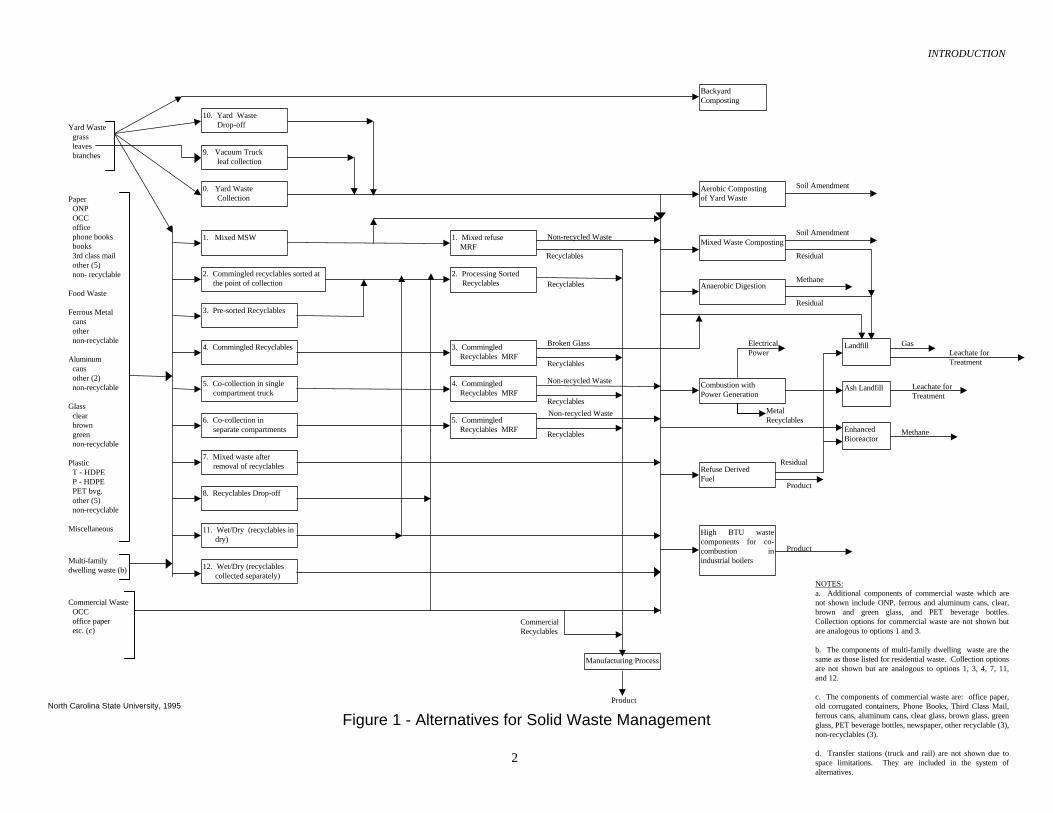
For the municipal official, agency or outside consultant responsible for makingrecommendations on the “best” way to manage the city or county’s solid waste, oneapproach is to first determine the types and amounts of waste generated by households,apartment dwellers, and commercial businesses. The next step would be to collect asmuch information as possible about all the options at each step in the waste managementprocess, including, collection of the waste, treatment, disposal, and, if applicable,transformation of waste into new products. Figure 1 is a network diagram showingalternative solid waste management options and how they can be “connected” to producean overall solid waste management program.
INTRODUCTION
2
North Carolina State University, 1995
Figure 1 - Alternatives for Solid Waste Management
NOTES:a. Additional components of commercial waste which arenot shown include ONP, ferrous and aluminum cans, clear,brown and green glass, and PET beverage bottles.Collection options for commercial waste are not shown butare analogous to options 1 and 3.
b. The components of multi-family dwelling waste are thesame as those listed for residential waste. Collection optionsare not shown but are analogous to options 1, 3, 4, 7, 11,and 12.
c. The components of commercial waste are: office paper,old corrugated containers, Phone Books, Third Class Mail,ferrous cans, aluminum cans, clear glass, brown glass, greenglass, PET beverage bottles, newspaper, other recyclable (3),non-recyclables (3).
d. Transfer stations (truck and rail) are not shown due tospace limitations. They are included in the system ofalternatives.
MetalRecyclables
Paper ONP OCC office phone books books 3rd class mail other (5) non- recyclable
Food Waste
Ferrous Metal cans other non-recyclable
Aluminum cans other (2) non-recyclable
Glass clear brown green non-recyclable
Plastic T - HDPE P - HDPE PET bvg. other (5) non-recyclable
Miscellaneous
Ash Landfill
LandfillLeachate forTreatment
Leachate forTreatment
Gas
BackyardComposting
Aerobic Compostingof Yard Waste
Refuse DerivedFuel
Combustion withPower Generation
ElectricalPower
Product
Yard Waste grass leaves branches
1. Mixed refuse MRF
9. Vacuum Truck leaf collection
10. Yard Waste Drop-off
Multi-familydwelling waste (b)
Recyclables
Recyclables
Non-recycled Waste
3. Commingled Recyclables MRF
2. Processing Sorted Recyclables
4. Commingled Recyclables MRF
5. Commingled Recyclables MRF
Commercial Waste OCC office paper etc. (c)
0. Yard Waste Collection
12. Wet/Dry (recyclables collected separately)
1. Mixed MSW
2. Commingled recyclables sorted at the point of collection
3. Pre-sorted Recyclables
4. Commingled Recyclables
5. Co-collection in single compartment truck
6. Co-collection in separate compartments
7. Mixed waste after removal of recyclables
8. Recyclables Drop-off
11. Wet/Dry (recyclables in dry)
Anaerobic Digestion
Manufacturing Process
Mixed Waste Composting
Product
High BTU wastecomponents for co-combustion inindustrial boilers
Product
Soil Amendment
Soil Amendment
Residual
Residual
Methane
Broken Glass
Recyclables
Non-recycled Waste
Non-recycled Waste
Recyclables
Recyclables
Residual
CommercialRecyclables
EnhancedBioreactor
Methane

INTRODUCTION
3
It would help to have a tool that would model as many of these options as possible,assemble various combinations of options into waste management strategies or scenarios,calculate the cost and life-cycle inventory (LCI) for each scenario that therecommendation will be based on, and then rank them from best to worst. Cost is themost obvious parameter on which to base such a recommendation, but there might besituations where another parameter is of overriding importance. For instance if reductionin CO2 emissions were a priority, then the lowest cost waste management scenario maynot be the optimal implementation.
The Decision Support Tool (DST) is a personal computer based decision making tool foranalyzing solid waste management alternatives using the LCI approach. This documentdescribes one component of the DST: the collection portion of an overall Excelspreadsheet that calculates costs and LCI parameters for MSW collection options. It isreferred to throughout this document as the “Collection Process Model”. It wasdeveloped for use with other “process model” portions of the spreadsheet that calculateLCI parameters for other waste management process options such as landfilling,composting, and combustion. Another component of the DST is a user interface thatallows a user to conveniently enter input data that enable the DST to closely modelcurrent or future characteristics of his or her city’s solid waste management program,including options that the city may be considering as alternatives. The other majorcomponent of the DST is a linear optimization module that analyzes the process modelLCI parameters (coefficients) and selects the optimum set of options for the LCIparameter that the user has designated for optimization. If the parameter is cost, then theDST selects options that produce the lowest overall solid waste management cost.Likewise, if the parameter is methane emissions, the DST selects options that togetheremit the least amount of methane.
The Collection process model is also designed as a tool that can be used independentlyfrom the DST. In this so called “stand alone” mode of operation, the Collection processmodel serves as a means for comparing the costs, energy usage rates, pollutant emissions,and other factors for 21 different MSW collection options. This gives the user theopportunity to see how changing the value of one input variable such as the length of acollection vehicle’s workday affects the number of vehicles needed to collect all of thecity’s waste and how, in turn, this affects the total annual cost of MSW collection.However, in this mode of operation, it must be understood that the resulting costs andLCI burdens are only representative of the case where all waste is collected by only asingle collection option or valid combination of options and that recycling occurs at themaximum dictated by factors such as participation rate . For example, the C1 (mixedwaste collection) costs and LCI burdens are only valid for collection of all waste andwould not be directly applicable to the case where a C3 recycling program wereimplemented for some fraction of a given residential sector. As such, use of this model inas a stand alone tool should be attempted only by a knowledgeable user.
INTRODUCTION
4
When operating in this stand alone mode, the Collection process model must access someof the information contained in several other process models: the Common processmodel, where solid waste composition data and demographic information such as thenumber of residential homes, multi-family dwellings (i.e., apartments), and commercialsites are stored; the Electrical Energy process model, which stores data on the water andair pollutant emissions associated with the consumption of electricity; the CollectionDistances process model, which stores distances to the various unloading locations towhich each of the collection options can be routed and the Collection by Sector processmodel which stores sector specific data for each of the 2 residential, 2 multi-family and10 commercial sectors defined in the model. The Collection process model contains linksto these sheets of the overall spreadsheet. Thus, if a new value for the number ofresidential households in a sector is input, all of the calculations in the Collection processmodel that use this particular variable are automatically updated.
The next chapter in this document, Methodology, describes what LCI parameters theCollection process model calculates and the approach and assumptions that thesecalculations are based on. Chapter 3, Collection Cost Equations, lists the equations andexplains the methodology used in the spreadsheet to calculate a city or county’s annualcost of collecting residential, multi-family, and commercial MSW as well as howinflation is accounted for. In addition, the Collection process model calculates three typesof unit costs: annual cost per collection vehicle, annual cost per collection location, andcost per ton of MSW. Chapter 3 covers each of the 21 collection options. Chapter 4describes calculation procedures for parameters such as daily collection vehicle mileageand fuel usage that are referenced in subsequent chapters. The equations used to calculateconsumption rates of energy and water associated with MSW collection are listed andexplained in Chapters 5 and 6, respectively. Chapters 7, 8, and 9 cover the calculation ofairborne pollutant release rates, waterborne pollutant release rates, and solid wastegeneration rates.
The Collection process model and the other process model that it accesses in stand alonemode each include a set of default input variable values. These values are drawn from avariety of sources and are intended to represent national averages. The DST or theCollection process model user has the option to override these default values with othervalues that represent more closely the solid waste management program that he or she istrying to model. The default input variable values for all Collection process modelcollection options are listed in Appendix A. Appendices B and C include default inputvalues for parameters that vary by sector and for those that vary by sector and “nextnode”, respectively. Appendix D lists the output values for all parameters that arecalculated by the Collection process model using the default input variable values.
Consumption and release rates for LCI parameters in the Collection process model areexpressed in terms of units of the consumption or release parameter (Btu’s of energy,pounds of pollutant, etc.) per ton of MSW. These rates and the unit costs of MSWcollection vary depending on the weight and density of the waste generated by city or

INTRODUCTION
5
county residents and commercial waste generators, which in turn depend on whichcomponents of the MSW stream are being collected by each collection method. Forinstance, the cost per ton to collect recyclables will be different depending on whether ornot old newsprint is included in the recyclables collection program. When used in standalone mode, the user can specify which MSW components are collected by each methodand their component weights and densities, or use the default input data values includedin the Collection and Common process models. However, one of the functions of theOptimization Module is to select the most economical, most energy efficient, or leastpolluting combination of components at each stage of the MSW management process,including collection. The Collection process model therefore includes sets of coefficientsfor costs and selected LCI consumption and release parameters for each MSW componentand collection option that are independent of the aggregate MSW weight and density.Appendix E lists the equations for these coefficients for collection costs and each of theLCI parameters.
Appendix F lists all variable names used in the Collection process model. Appendix Gincludes cost escalation data used to account for inflation.

METHODOLOGY
6
2. METHODOLOGY
The methodology used in the Collection process model to calculate the number ofcollection vehicles needed to service all the collection locations in a city or county andthe cost to collect the waste generated at those locations is modeled after the equationsdeveloped by Kaneko (1995). Kaneko’s method starts by determining the number ofcollection locations that a collection vehicle can stop at along a collection route before itis filled to capacity. This number, multiplied by the amount of time that a vehicle spendsstopped at each location and traveling between locations, yields the length of time that acollection vehicle takes to travel from the beginning to the end of its collection route.The length of time that a collection vehicle takes to make a complete collection tripincludes the route travel time plus time spent traveling back and forth from the locationwhere it unloads the material that it collects (landfill, Material Recovery Facility,composting facility, etc.) and the time spent unloading at that location. Many inputs thatflow into these calculations will vary depending on the characteristics of the sector beingcollected (MSW composition, etc.) and the average distance from that sector to each ofthe several possible unloading facilities. The implications of different collection sectorsand unloading locations are addressed in Sections 2.1 and 0, respectively.
At this point in the calculation procedure it is possible to iteratively determine the integernumber of fully loaded trips that a collection vehicle can make during one workday, aftertime is deducted for travel to and from the vehicle garage at the end of each day and thebeginning of the next day and for the lunch break and other break time. However, it isnot feasible to express the iterative calculations in the form of a cost or LCI parametercoefficient cell formula, which is the format that is required for interface with the DSTOptimization Module. For this reason, Kaneko developed an equation which calculates anon-integer number of daily collection vehicle trips. This equation closely approximatesthe integer value for daily collection trips. Given the other approximations which mustbe made to calculate collections costs and other LCI parameters such as rates of MSWgeneration and vehicle travel and loading/unloading times, the use of a non-integer valuefor daily collection vehicle trips does not significantly affect the accuracy of theCollection Preprocess output data.
The next step is to divide the total number of collection locations in the area served by acollection option by the number of collection locations that a vehicle stops at during onecollection trip to determine the total number of trips needed to collect all the MSWgenerated in that area during on collection cycle. (A collection cycle may represent oneor more visits to each collection site per week, with a default value of one visit per week).When used in stand alone mode, the Collection process model offers the user the optionof dividing the city or county being modeled into areas that are served by differentcollection options. This is done by means of the option_frac input variable. If the userenters and option_frac value of 1.00 for a particular collection option, say for C1
METHODOLOGY
7
(residential curbside mixed waste collection), then 100% of the households in the city orcounty would be served by option C1 collection vehicles. If, however, the user wished tomodel a situation where half of the neighborhoods in a city are served by mixed wastecollection and the other half set out their recyclables in a bin for collection by acommingled recyclables collection vehicle (option C4), then he or she would specifyoption_frac values of 0.50 for option C1 and C4. The Collection Processor uses thesevalues to calculate the required number of C1, C4, and C7 (collection of residual wastefrom locations served by option C4) collection trips. It should be noted that theoption_frac values are relevant only in stand-alone mode. When the optimization modelis used, the fraction of households collected be each collection option will be dictated bethe model solution based on the user’s optimization criteria (minimum cost, CO2, etc.).
Once the numbers of daily collection vehicle trips and total collection trips are known, thenumber of trucks is determined by dividing total trips by daily trips and by the number ofdays per week that collection vehicles operate. (This also produces a non-integer valuewhich is considered adequate for use with the Decision Support System.) Then annualMSW collection cost is found by multiplying the number of trucks by economic factorsincluding a vehicle’s annualized capital cost based on the purchase price amortized overservice life, vehicle operating costs, labor costs, overhead costs, and costs for backupvehicles and collection crew personnel as well as factors to account for inflation from thebase year for which the default cost data were collected.
Unit costs for MSW collection (annual cost per collection vehicle, annual cost percollection location, and cost per ton MSW collected) are independent of the number ofcollection vehicles. The annual collection cost per vehicle is determined for eachcollection option using the economic factors listed above. The annual cost per collectionlocation is found by dividing the annual vehicle cost by the number of locations visited byeach vehicle during one collection cycle. The cost per ton of MSW collected is found bydividing the annual cost per collection location by the number of tons of MSW generatedper year by the residents or commercial businesses whose waste is collected at thatcollection.
The Collection process model spreadsheet includes a calculation section that breaks downthe collection vehicle workday into the number of minutes that a vehicle is used for eachtask. Default or user override values for the speed that a vehicle travels while performingdifferent tasks and its fuel consumption rate are used to determine how many miles ittravels and how many gallons of fuel it consumes per day. (Similar calculations areperformed for the two collection options that model residents’ use of their own vehiclesto drop off recyclables or yard waste at designated drop-off sites.) These in turn aremultiplied by pollutant emission factors and energy content factors to arrive at values forthe amounts of energy, and maintenance items consumed and the amount of airpollutants, water pollutants, and solid wastes generated per ton of waste collected. TheLCI parameter calculations also include the consumption of electrical energy at the garagewhere the collection vehicles are stored and maintained when not in service. The water

METHODOLOGY
8
pollutant, air pollutant, and solid waste generation rates also include the pollutants andsolid wastes associated with the generation of electrical energy consumed at the garage.
METHODOLOGY
9
2.1 Collection Sectors
In order to allow for the likelihood that certain parameters such as MSW compositionmight vary between geographic subsections of the entity being modeled (city, county,etc.) and for similar variations between commercial business types, multiple sectors canbe modeled simultaneously. The model provides for 2 residential sectors, 2 multi-familysectors and 10 commercial sectors. While the user can only examine one sector of eachtype (residential, multi-family and commercial) using the stand-alone method, theoptimization model increments through all sectors and their related sector variableparameters to gather cost and LCI coefficients for each sector for optimization. This isyet another example of the previously stated caution that stand-alone use of the collectionprocess model should be used only with great caution and by a user that is familiar withthe applicability of the resulting values.
Variables which vary by collection sector include the following list of variables, all ofwhich are defined in Appendix F:
HS, Fr, TL, Tbtw, Trf, Tgr, Tfg, Nw, Vt, Lt, Pt, c, Vbet, Vgr, Dbet, Dgr, res_pop, ph, gr,h_res, g_res, mf_pop, mf_gen, h_mf, g_mf, h_com, g_com, RES_WT_FRAC,MF_WT_FRAC, COM_WT_FRAC, option_frac

METHODOLOGY
10
2.2 Collection “Next Node”
The distance to the unloading location (landfill, MRF, etc.) will affect the cost since adifferent number of vehicles will be required depending on this distance. Likewise, theLCI burden will vary depending on the amount of time that collection vehicles aretraveling to these various locations. Since the destination to which MSW and recyclablesare taken after collection will affect cost and LCI coefficients, the optimization modelmust have a set of coefficients for each unloading location or “next node”. As such, theuser must define the average distance (for each sector) from the collection sector to eachpossible facility to which the collected material can be routed. These inputs for thesedistances for all sectors are shown in Appendix C.
While the user can only examine one unloading location (or “next node”) using the stand-alone method, the optimization model increments through all “next nodes” and theirrelated distances for each sector to gather cost and LCI coefficients for optimization.This is yet another example of the previously stated caution that stand-alone use of thecollection process model should be used only with great caution and by a user that isfamiliar with the applicability of the resulting values.
Variables which vary by collection sector and “next node” include the following list ofvariables, all of which are defined in Appendix F:Trf, Tfg, Vrf, Vfg, Drf, Dfg
COLLECTION COST EQUATIONS
11
3. COLLECTION COST EQUATIONS
The Collection process model calculates the following four unit costs for 20 of the 21waste collection options:
(a) collection cost per year(b) collection cost per collection vehicle per year(c) collection cost per collection location per year(d) collection cost per ton of refuse collected
[Option C10, Yard Waste Drop-Off, does not incur any costs for purchase oroperation of municipal collection vehicles. Therefore, no unit costs are calculated forthis collection option.]
Unit cost (a), collection cost per year, is determined by calculating the number ofmunicipal collection vehicles and containers that are used to collect the waste generatedby community residents, then multiplying the totals by the annualized vehicle andcontainer costs. As explained below, the user can specify whether the entire communityis served by a particular collection option, or only a fraction of the community.Collection cost per year is a function of the number of residents served by that collectionoption.
Unit costs (b), (c), and (d) are independent of the number of residents served by aparticular collection option. Unit cost (b), collection cost per collection vehicle per year,is the sum of the annualized capital and operating costs for one collection vehicle plus theannualized capital cost of any containers provided to the residents at collection locationsserviced by that vehicle.
Unit cost (c), collection cost per collection location per year, is the sum of the annualizedcosts for one collection vehicle divided by number of collection locations serviced by thatvehicle plus the annualized cost of any containers provided to the residents at thoselocations. “Collection location” refers to single family households for residential wastecollection options. For multi-family waste collection options, “collection location” refersto groups of multi-family dwellings whose residents deposit their waste at a singlecollection container.
Unit cost (d), collection cost per ton of refuse collected, is found by dividing unit cost (c)by the weight (in tons) of waste generated during one year by the residents whose waste iscollected at one collection location.
Only unit cost (d), collection cost per ton of refuse collected, is used by the OptimizationModel when it is seeking a lowest cost waste management strategy. The other three unit

COLLECTION COST EQUATIONS
12
costs are provided for the convenience of the user when using the Collection processmodel in a stand-alone mode to compare costs of different collection options.

COLLECTION COST EQUATIONS
13
3.1 Cost Escalation
All default costs for the collection model are based on 1993 data. In order to have thesedefault values reflect inflation to the year in which the model is being run, all defaultcosts are multiplied by a factor based on the Producer Price Index values for capitalequipment (USBLS, 1996). This escalation factor is:
1993_
___
CIyearcurCI
FactorCI = ,
where:
=FactorCI _ Cost index factor used to inflate 1993 costs. =yearcurCI __ Cost index factor for the year indicated by the computer
0perating system or the override year entered by the modeluser (see Appendix E)
=1993_CI Cost index factor for 1993 (see Appendix E).
All costs referenced in this document are treated in this way.
COLLECTION COST EQUATIONS
14
3.2 Residential Waste Collection
Residents living in single family dwellings (“households”) can be served by one or moreof the 10 residential waste collection options included in the Collection process model.They are assumed to dispose of their refuse in their own containers. Some collectionoptions allow for additional containers that are provided to each household at communityexpense, in which residents can dispose of recyclables separately from the rest of theirrefuse.
The general pattern for residential waste collection proceeds as follows: Collectionvehicles leave from a vehicle garage at the beginning of each workday to begin collectingresidential refuse along predetermined routes. The length of a collection route isdetermined by the number of households that a vehicle can service before it is filled tocapacity. Fully loaded vehicles drive to a treatment or disposal facility, unload, and driveback to the starting point of another collection route. At the end of the workday thevehicles travel from the treatment or disposal facility back to the vehicle garage.
The default value for frequency of waste collection is once per week. (The user canspecify more or less frequent collection frequencies based on fractions or multiples ofweeks.) For that reason, many of the cost calculations in the Collection process modelinclude a parameter for the amount of waste generated per week at each collectionlocation. The Collection process model calculates this parameter from values specifiedby the user for the number of residents living in single family households (res_pop), thetotal number of single family households in the community (H_res), and the residentialper capita waste generation rate (GR). The Collection process model calculates theaverage weekly waste generation rate per household (G_res) using the formula:
resHpopresGR
resG weekdays
_
7__
××= ,
where:
G res_ = waste generated per residential household (pounds per household per week)
GR = waste generated per resident per day (pounds per person per day)
res pop_ = number of people living in residential households (persons) H res_ = number of residential households (households)

COLLECTION COST EQUATIONS
15
3.2.1 Mixed Waste (C1)
The Mixed Waste cost equations used in Collection Option C1 calculate the cost tocollect residential mixed solid waste in single compartment collection vehicles. Thewaste is not separated into different components such as recyclables and non-recyclablesat the point of collection. No special containers are provided to residents, so collectioncosts are only associated with purchase and operation of collection vehicles.
3.2.1.1 Generation Rate
One of the parameters used to calculate Mixed Waste collection costs is the weeklyhousehold mixed solid waste generation rate (G_msw). Since there is no waste separationat the point of collection, the value of G_msw for Collection Option C1 is the same as theweekly residential waste generation rate G_res calculated by the Collection processmodel:
G msw G res_ _=
3.2.1.2 Waste Density
Default values for the compacted density of individual components of the waste streamare listed in the Collection process model (D_cv). The Collection process model usesthese values and the default values of the individual component weight fractions forresidential waste sector 1 listed in the Common process model (RES_WT_FRAC_1) tocalculate an overall density for residential mixed waste:
D msw RES WT FRACD cv
i
ii
_ _ _ __
=∑
11 ,
where:
D msw_ = overall density of mixed waste (pounds per cubic yard) RES WT FRAC i_ _ _1 = weight fraction for waste component i of the Sector 1
residential waste composition D cvi_ = compacted density of waste component i
This value represents the overall density of the waste after compaction in the collectionvehicle.
D_msw can also be specified by the user. This is done by entering the desired value incell d_msw in the Option C1 column of the Input Parameters section of the Collection

COLLECTION COST EQUATIONS
16
process model. Entering a value in this cell overrides the calculation procedure describedabove, and the Collection process model uses the user-specified density value in allsubsequent calculations. If the d_msw cell is empty, the Collection process modelcalculates the overall density and uses the calculated value in subsequent calculations.
3.2.1.3 Cost Equations
The steps used to calculate residential curbside collection costs are as follows: 1. Number of households that a collection vehicle can stop at to collect mixed waste
refuse before it is filled to capacity. This represents the number of households that avehicle can service along a collection route during one collection trip.
( )HtUt Vt Fr
G msw D msw=
× ×_ _
,
where: Ht = number of households serviced per collection trip
(households per trip) Ut = collection vehicle utilization factor (useable cubic yards of
vehicle capacity per total cubic yards of vehicle capacity) Vt = collection vehicle capacity (cubic yards per trip)
D msw_ = overall density of mixed waste (pounds per cubic yard) Fr = collection frequency (collection cycles per week)
G msw_ = mixed waste generation rate (pounds per week per household)
2. Travel time from the vehicle garage to the starting point of the first collection route(Tgr). (Collection vehicles are assumed to remain parked at a garage/maintenancefacility overnight between the end of one workday and the beginning of the nextworkday.)
Tgr can be specified by the user (default value: 20 minutes). If there is no valueentered in the Tgr cell or if the value in the Tgr input cell is zero, the Collectionprocess model calculates a value for Tgr using user-specified or default values for thedistance from the garage to the collection route starting point (Dgr) and the averagespeed that the vehicle travels over this distance (Vgr). Default values for Dgr and Vgrare 11.67 miles and 35 miles per hour, respectively. The Collection process modelthen calculates Tgr as:
TgrDgrVgr
minhr= × 60 ,
COLLECTION COST EQUATIONS
17
where:Tgr = travel time from garage to start of first collection route
(minutes per day per vehicle)Dgr = distance from garage to start of first collection
route (miles per day per vehicle)Vgr = average travel speed between garage and start of first
collection route (miles per hour)
3. Length of time to travel between collection stops (Tbet).
Tbet can be specified by the user (default value: 0.17 minutes). If there is no valueentered for Tbet or if the value in the Tbet input cell is zero, the Collection processmodel calculates a value for Tbet using user-specified or default values for theaverage distance between collection stops (Dbet) and the average speed that thevehicle travels over this distance (Vbet). Default values for Dbet and Vbet are 0.0142miles (75 feet) and 5 miles per hour, respectively. The Collection process model thencalculates Tbet as:
TbetDbetVbet
minhr= × 60 ,
where:Tbet = travel time between collection stops (minutes/stop)Dbet =distance between collection stop (miles)Vbet = average travel speed collection stops (miles per hour)
4. Travel time between the start/end of a collection route and the disposal facility (Trf).(The Collection process model calculations assume that a collection vehicle takes thesame amount of time to travel from the end of a collection route to the disposalfacility as it does to travel from the disposal facility to the start of its next collectionroute.)
Trf can be specified by the user (default value: 20 minutes). If there is no valueentered for Trf or if the value in the Trf input cell is zero, the Collection processmodel calculates a value for Trf using user-specified or default values for the distancefrom the end of the collection route to the facility (Drf) and the average speed that thevehicle travels over this distance (Vrf). Default values for Drf and Vrf are 10 milesand 30 miles per hour, respectively. The Collection process model then calculates Trfas:
TrfDrfVrf
minhr= × 60 ,
COLLECTION COST EQUATIONS
18
where:Trf = travel time between start/end of collection route and the
disposal facility (minutes per trip)Drf = distance between start/end of a collection route and the
disposal facility (miles)Vrf = average travel speed between start/end of collection route
and the disposal facility (miles per hour)
5. Travel time from the disposal facility to the vehicle garage at the end of the workday(Tfg).
Tfg can be specified by the user (default value: 20 minutes). If there is no valueentered for Tfg or if the value in the Tfg input cell is zero, the Collection processmodel calculates a value for Tfg using the user-specified or default values for thedistance from the disposal facility to the (Dfg) and the average speed that the vehicletravels over this distance (Vfg). Default values for Dfg and Vfg are 11.67 miles and35 miles per hour, respectively. The Collection process model then calculates Tfg as:
TfgDfgVfg
minhr= × 60 ,
where:Tfg = travel time from disposal facility to garage at the end of the
workday (minutes per day per vehicle)Dfg = distance from disposal facility to the garage (miles per day
per vehicle)Vfg = average travel speed between disposal facility and garage
(miles per hour)
6. Length of time that it takes a collection vehicle to make one collection trip (Tc),including time spent traveling from a disposal facility to the beginning of thecollection route, loading waste at collection stops, traveling to the disposal facility atthe end of the trip, and unloading the vehicle at the disposal facility.
( )[ ] ( )[ ] ( )Tc Tbet HtHS TL Ht
HS Trf S= × − + × + × +1 2 ,
where: Tc = collection trip time (minutes per trip)Tbet = travel time between collection stops (minutes per stop) Ht = number of households serviced per collection trip
(households per trip)

COLLECTION COST EQUATIONS
19
HS = number of households from which refuse is collected at onecollection stop (households per stop)
TL = loading time at a collection stop (minutes per stop) Trf = travel time between beginning/end of collection route and
disposal facility (minutes per trip) S = time to unload collection vehicle at the disposal facility
(minutes per trip)
7. Number of collection trips that a vehicle can make during one workday after time isdeducted for a lunch period, other breaks, and travel to and from the vehicle garage.
( ) ( ) ( )[ ]RD
WV F F Tgr Tfg Trf S
Tc=
× − + + + − × +60 1 2 0 5. ,
where: RD = collection trips per day per vehicle (trips per day per
vehicle) WV = work hours per workday (hours per day per vehicle) F1 = lunch period (minutes per day per vehicle) F2 = break period (minutes per day per vehicle) Tgr = travel time between garage and beginning of collection
route (minutes per day per vehicle)Tfg = travel time between disposal facility and garage (minutes
per day per vehicle)
8. Number of collection vehicle trips needed to service all of the households served bycollection option C1.
RTH res option frac
Ht=
×_ _ ,
where: RT = number of collection trips needed (trips) H res_ = number of households in the community (households)
option frac_ = fraction of households served by collection option C1 Ht = number of households serviced per collection trip
(households per trip)
9. Number of collection vehicles needed to visit all of the households served bycollection option C1 during one collection cycle:
NtRT
RD
Fr
CD= × ,

COLLECTION COST EQUATIONS
20
where: Nt = number of collection vehicles CD = number of workdays per week (days per week)
10. Annual capital (C_cap_v) and operating (C_op) costs associated with a singlecollection vehicle:
Capital Cost
( )C cap v e Pt CRF_ _ = + × ×1 ,
where: C cap v_ _ = collection vehicle capital cost amortized over the economic
life of the vehicle ($ per vehicle per year) e = administrative rate ($ of administrative expense per $ of
capital or operating cost) Pt = unit price of a collection vehicle ($ per vehicle)CRF = capital recovery factor for a collection vehicle (year-1)
The capital recovery factor is defined as:
( )( )
CRFi i
i
L
L=× ++ −
1
1 1 ,
where: i = yearly discount rate (year-1) L = economic life of a collection vehicle (years)
Operating Cost
( ) ( ) ( ) ( ) ( )[ ]C e a bw Wa Nw Wd WP CD c d Nwopdays
year
daysweek
_ = + × + × + × × + × × ×
+ + × +
1 1 1
365
71
where: C op_ = collection vehicle operating cost per year ($ per vehicle per
year) a = fringe benefit rate ($ of fringe benefits per $ of wages)
bw = backup rate for collection workers (backup worker per collection worker)
Wa = hourly wage rate for collection worker ($ per hour per worker)

COLLECTION COST EQUATIONS
21
Nw = number of collection workers per vehicle (workers) Wd = hourly wage rate for a collection vehicle driver ($ per hour
per driver) WP = work hours per day for wage (hours per worker per day) c = annual vehicle operation and maintenance cost ($ per year
per vehicle) d = other expenses ($ per worker per year)
11. Annual collection cost per vehicle:
( )[ ]C vehicle bv C cap v C op_ _ _ _= + × +1 ,
where: vehicle ction cost per collection vehicle ($ per
vehicle per year)bv = backup rate for collection vehicles (backup vehicle per
collection vehicle)
12. Total annual collection cost for the community:
C ann Nt C vehicle_ _= × ,
where: C ann_ = total annual collection cost ($ per year)
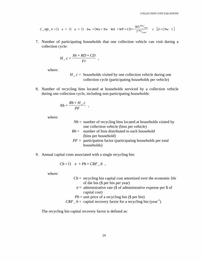
13. Number of households that one collection vehicle can visit during a collection cycle:
H cHt RD CD
Fr_ =
× × ,
where: H c_ = households visited by one collection vehicle during one
collection cycle (households per vehicle)
14. Collection cost per household per year:
C houseC vehicleH c HS
__
_=
× ,
where:
COLLECTION COST EQUATIONS
22
C house_ = annual collection cost per household ($ per household per year)
15. Collection cost per ton of refuse:
C tonC house
G msw
lbton
daysweek
daysyear
__
_=
× ××
2000 7
365 ,
where: C ton_ = collection cost per ton of refuse ($ per ton)
COLLECTION COST EQUATIONS
23
3.2.2 Recyclables (C2, C3, and C4)
Options C2, C3, and C4 model collection of recyclables which have been separated fromthe non-recyclable portion of residential refuse (“residuals”) and set out by residents forcollection. Each household can be supplied with one or more containers (“bins”) to holdtheir recyclable refuse. The user can specify both the number of containers supplied perhousehold and the unit price of any containers that are supplied at community expense.The annualized capital cost of the bins is treated as an additional capital collection cost.The default values for the number of recyclables containers included in the InputParameter section of the Collection process model are discussed below. [Note: TheCollection process model assumes that containers are supplied to all households in thesection of the community served by a recyclables collection option regardless of whetherthey elect to participate in the recycling program or not.]
The cost equations for options C2, C3, and C4 are identical; differences in collectioncosts among the three options are due to differences in the values of input data such as thenumber of recycling bins supplied to each household, the time to load (and, in some casesseparate) recyclables at collection stops, the number of workers in the vehicle crew, andthe collection vehicle capital and operating costs. The recyclables collection options aredescribed as follows:
• Option C2 models collection of commingled recyclables set out in a single bin. Therecyclables in the bin are sorted by the collection vehicle crew at the time ofcollection and loaded into separate compartments of a multi-compartment collectionvehicle.
• Option C3 covers collection of pre-sorted recyclables set out in multiple bins. Thecollection crew empties each bin into the appropriate compartment of a multi-compartment collection vehicle. The default value for the number of bins is five perhousehold.
• Option C4 models collection of commingled recyclables set out in a single bin. Thecollection crew empties the bin into a single compartment collection vehicle. It isassumed that residents separate their old newspapers from their other recyclables andthat these are loaded into a separate compartment of the collection vehicle.
3.2.2.1 Generation Rate
The weekly household generation rate for recyclables (G_recyc) is found by multiplyingthe total weekly household waste generation rate (G_res) by the fraction of recyclablesremoved, or “captured”, from the waste stream (frac_cap_recyc). When the Collectionprocess model is used with the Optimization Model, the Optimization Model determineswhich components of the waste stream are collected by a particular collection option.
COLLECTION COST EQUATIONS
24
When the Collection process model is used in stand-alone mode, the user specifies whichcomponents are collected. This procedure is described below.
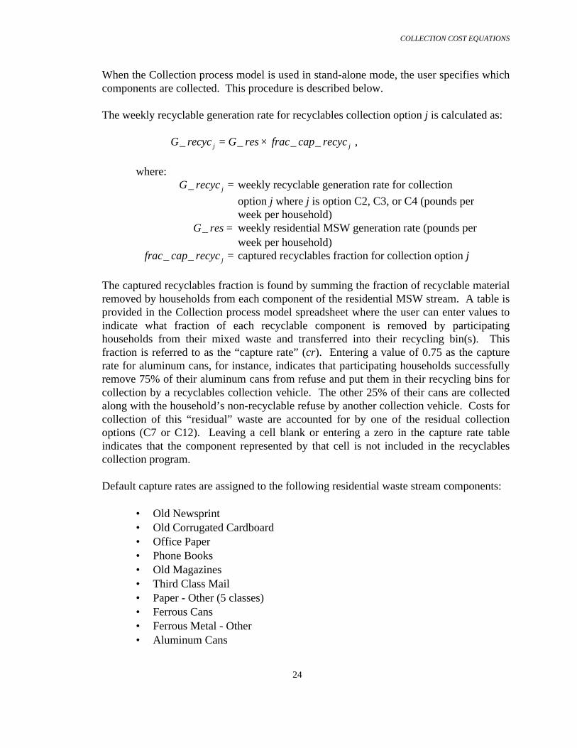
The weekly recyclable generation rate for recyclables collection option j is calculated as:
G recyc G res frac cap recycj j_ _ _ _= × ,
where: G recyc j_ = weekly recyclable generation rate for collection
option j where j is option C2, C3, or C4 (pounds per week per household)
G res_ = weekly residential MSW generation rate (pounds per week per household)
frac cap recyc j_ _ = captured recyclables fraction for collection option j
The captured recyclables fraction is found by summing the fraction of recyclable materialremoved by households from each component of the residential MSW stream. A table isprovided in the Collection process model spreadsheet where the user can enter values toindicate what fraction of each recyclable component is removed by participatinghouseholds from their mixed waste and transferred into their recycling bin(s). Thisfraction is referred to as the “capture rate” (cr). Entering a value of 0.75 as the capturerate for aluminum cans, for instance, indicates that participating households successfullyremove 75% of their aluminum cans from refuse and put them in their recycling bins forcollection by a recyclables collection vehicle. The other 25% of their cans are collectedalong with the household’s non-recyclable refuse by another collection vehicle. Costs forcollection of this “residual” waste are accounted for by one of the residual collectionoptions (C7 or C12). Leaving a cell blank or entering a zero in the capture rate tableindicates that the component represented by that cell is not included in the recyclablescollection program.
Default capture rates are assigned to the following residential waste stream components:
• Old Newsprint• Old Corrugated Cardboard• Office Paper• Phone Books• Old Magazines• Third Class Mail• Paper - Other (5 classes)• Ferrous Cans• Ferrous Metal - Other• Aluminum Cans

COLLECTION COST EQUATIONS
25
• Aluminum - Other (2 classes)• Clear Glass• Brown Glass• Green Glass• Translucent HDPE• Pigmented HDPE• PET• Plastic - Other (5 classes)
The Common process model contains tables of waste component weight fractions for twodifferent residential waste compositions representing different sectors of the community(RES_WT_FRAC_1 and RES_WT_FRAC_2). To determine frac_cap_recyc theCollection process model worksheet multiplies the user-specified/default capture rate foreach waste component by the corresponding weight fraction specified for that componentin the RES_WT_FRAC_1 table.
frac cap recyc cr RES WT FRACj iji
i_ _ _ _ _= ×∑ 1 ,
where:
frac cap recyc j_ _ = captured recyclables fraction for collection option j
where j is C2, C3, or C4 crij = capture rate for waste component i for collection option j
RES WT FRAC i_ _ _1 = weight fraction for waste component i of the Sector 1 residential waste composition
3.2.2.2 Waste Density
Default values for the as-collected density of recyclable components of the residentialwaste stream are listed in the Common process model (D_rcv). Default values for wastecomponent compaction factors (CF) are listed in the Input Parameters section of theCollection process model. Compaction factors represent the increased density of anywaste components that are compacted during collection. The default compaction factorvalues for all waste components are 1.0. The Collection process model uses these valuesand the default values of the individual component weight fractions for residential wasteSector 1 listed in the Common process model (RES_WT_FRAC_1) to calculate an overalldensity for residential recyclables in a recyclables collection vehicle.
D recycfrac cap recyc
cr RES WT FRAC
D rcv CF
j
j
ij i
i iji
__ _
_ _ _
_
= ×
×∑ 1
,
COLLECTION COST EQUATIONS
26
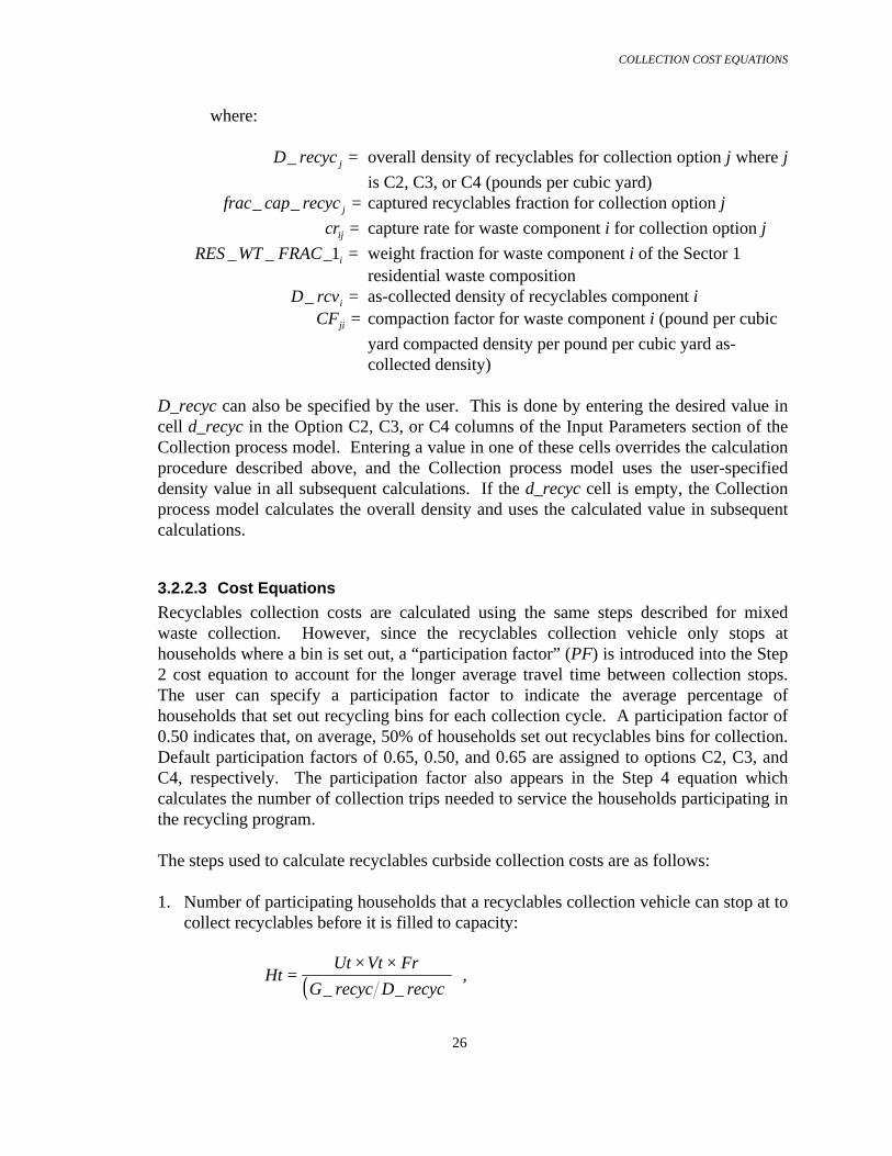
where:
D recyc j_ = overall density of recyclables for collection option j where j
is C2, C3, or C4 (pounds per cubic yard) frac cap recyc j_ _ = captured recyclables fraction for collection option j
crij = capture rate for waste component i for collection option j
RES WT FRAC i_ _ _1 = weight fraction for waste component i of the Sector 1 residential waste composition
D rcvi_ = as-collected density of recyclables component iCFji = compaction factor for waste component i (pound per cubic
yard compacted density per pound per cubic yard as-collected density)
D_recyc can also be specified by the user. This is done by entering the desired value incell d_recyc in the Option C2, C3, or C4 columns of the Input Parameters section of theCollection process model. Entering a value in one of these cells overrides the calculationprocedure described above, and the Collection process model uses the user-specifieddensity value in all subsequent calculations. If the d_recyc cell is empty, the Collectionprocess model calculates the overall density and uses the calculated value in subsequentcalculations.
3.2.2.3 Cost Equations
Recyclables collection costs are calculated using the same steps described for mixedwaste collection. However, since the recyclables collection vehicle only stops athouseholds where a bin is set out, a “participation factor” (PF) is introduced into the Step2 cost equation to account for the longer average travel time between collection stops.The user can specify a participation factor to indicate the average percentage ofhouseholds that set out recycling bins for each collection cycle. A participation factor of0.50 indicates that, on average, 50% of households set out recyclables bins for collection.Default participation factors of 0.65, 0.50, and 0.65 are assigned to options C2, C3, andC4, respectively. The participation factor also appears in the Step 4 equation whichcalculates the number of collection trips needed to service the households participating inthe recycling program.
The steps used to calculate recyclables curbside collection costs are as follows:
1. Number of participating households that a recyclables collection vehicle can stop at tocollect recyclables before it is filled to capacity:
( )HtUt Vt Fr
G recyc D recyc=
× ×_ _
,

COLLECTION COST EQUATIONS
27
where: Ht = number of participating households serviced per collection
trip (participating households per trip) Ut = collection vehicle utilization factor
Vt = usable collection vehicle capacity (cubic yards per trip) Fr = collection frequency (collection cycles per week)
D recyc_ = overall density of recyclables (pounds per cubic yard) G recyc_ = recyclables generation rate (pounds per week per
participating household)
2. Length of time that it takes a collection vehicle to make one collection trip:
( )[ ] ( )[ ] ( )Tc TbetPF
HtHS TL Ht
HS Trf S= × − + × + × +1 2 ,
where: Tc = collection trip time (minutes per trip)Tbet = travel time between collection stops (minutes per stop) PF = participation factor (participating households per total
households) Ht = number of participating households serviced per collection
trip (participating households per trip) HS = number of households from which refuse is collected at one
collection stop (households per stop) TL = loading time at a collection stop (minutes per stop) Trf = travel time between beginning/end of collection route and
disposal facility (minutes per trip) S = time to unload collection vehicle at the disposal facility
(minutes per trip)
3. Number of collection trips that a vehicle can make during one workday:
( ) ( ) ( )[ ]RD
WV F F Tgr Tfg Trf S
Tc=
× + + + + + × +60 1 2 0 5. ,
where:RD = collection trips per day per vehicle (trips per day per
vehicle)
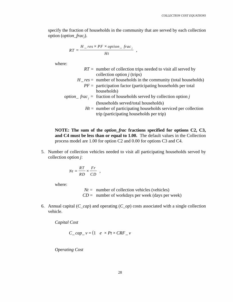
4. Number of collection vehicle trips (RT) needed to visit all of the participatinghouseholds in the community served by recyclables collection option j. Since theCollection process model includes three recyclables collection options, the user can
COLLECTION COST EQUATIONS
28
specify the fraction of households in the community that are served by each collectionoption (option_fracj).
RTH res PF option frac
Ht
j=× ×_ _
,
where: RT = number of collection trips needed to visit all served by
collection option j (trips) H res_ = number of households in the community (total households)
PF = participation factor (participating households per total households)
option frac j_ = fraction of households served by collection option j
(households served/total households) Ht = number of participating households serviced per collection
trip (participating households per trip)
NOTE: The sum of the option_frac fractions specified for options C2, C3,and C4 must be less than or equal to 1.00. The default values in the Collectionprocess model are 1.00 for option C2 and 0.00 for options C3 and C4.
5. Number of collection vehicles needed to visit all participating households served bycollection option j:
NtRT
RD
Fr
CD= × ,
where: Nt = number of collection vehicles (vehicles)CD = number of workdays per week (days per week)
6. Annual capital (C_cap) and operating (C_op) costs associated with a single collectionvehicle.
Capital Cost
( )C cap v e Pt CRF v_ _ _= + × ×1
Operating Cost
COLLECTION COST EQUATIONS
29
( ) ( ) ( ) ( ) ( )[ ]C e a bw Wa Nw Wd WP CD c d Nwop vdays
year
daysweek
_ _ = + × + × + × × + × × ×
+ + × +
1 1 1
365
71
7. Number of participating households that one collection vehicle can visit during acollection cycle:
H cHt RD CD
Fr_ =
× × ,
where: H c_ = households visited by one collection vehicle during one
collection cycle (participating households per vehicle)
8. Number of recycling bins located at households serviced by a collection vehicleduring one collection cycle, including non-participating households:
NbRb H c
PF=
× _ ,
where: Nb = number of recycling bins located at households visited by
one collection vehicle (bins per vehicle) Rb = number of bins distributed to each household
(bins per household) PF = participation factor (participating households per total
households)
9. Annual capital costs associated with a single recycling bin:
( )Cb e Pb CRF b= + × ×1 _ ,
where: Cb = recycling bin capital cost amortized over the economic life
of the bin ($ per bin per year) e = administrative rate ($ of administrative expense per $ of
capital cost) Pb = unit price of a recycling bin ($ per bin)
CRF b_ = capital recovery factor for a recycling bin (year-1)
The recycling bin capital recovery factor is defined as:

COLLECTION COST EQUATIONS
30
( )( )
CRF bi i
i
Lb
Lb_ =× ++ −
1
1 1 ,
where: i = yearly discount rate (year-1) Lb = economic life of a recycling bin (years)
10. Annualized capital cost of bins located at households serviced by one collectionvehicle, including those at non-participating households:
C cap b Cb Nb_ _ = × ,
where: C cap b_ _ = annualized capital cost of recycling bins at households
visited by one collection vehicle ($ per vehicle per year)
11. Collection cost per vehicle per year:
( )C vehicle bv C cap v C cap b C op_ _ _ _ _ _= + × + +1
12. Total annual collection cost for the community:
C ann Nt C vehicle_ _= ×
13. Collection cost per household per year:
C houseC vehicle PF
H c_
_
_=
×
14. Collection cost per ton of recyclables:
C tonC house
G recyc PF
lbton
daysweek
daysyear
__
_=
× ×× ×2000 7
365

COLLECTION COST EQUATIONS
31
3.2.3 Yard Waste (C0 and C9)
The Collection process model includes two options for collection of residential yardwaste. Option C0 models curbside collection of miscellaneous yard waste (leaves, grassclippings, branches) in a single compartment vehicle. Option C9 models curbsidecollection of leaves only using a leaf vacuum truck. Vehicles transport the collected yardwaste to a composting, combustion, anaerobic digestion, or enhanced bioreactor facilityor to a landfill, as determined by the Optimization Model.
The user can specify which components of residential MSW are collected, the capturerates that apply to these components, and the participation factor that applies to each yardwaste collection option. These are used to calculate the fraction of the total yard wastegenerated by residential households that is set out for collection.
3.2.3.1 Generation Rate
The generation rate for yard waste (G_yw) is a function of two variables: the total weeklyhousehold waste generation rte (G_res) and the amount of yard waste removed from thewaste stream (frac_yw). The user can specify these variables by entering values in theappropriate cells in the Collection process model worksheet to override the process modeldefault values.
The captured yard waste fraction (frac_yw) is found by summing the fraction of materialremoved by households from the yard waste components of the residential MSW stream.A table is provided in the Collection process model worksheet where the user can enter avalue to indicate what fraction on average of each yard waste component is removed byparticipating households from their mixed waste and set out for separate collection. Thisfraction is referred to as the “capture rate” (cr). Leaving a cell blank or entering a zero inthe capture rate table indicates that the component represented by that cell is not includedin the yard waste collection program.
For option C0, default capture rates are assigned to the following components:
• Leaves• Grass clippings• Branches
For option C9 a default capture rate is assigned to the Leaves component only.
The Common process model contains listings of waste component weight fractions fortwo residential waste compositions. To determine frac_yw the Collection process modelspreadsheet multiplies the user-specified/default capture rate for each yard waste

COLLECTION COST EQUATIONS
32
component by the corresponding Sector 1 weight fraction specified for that component inthe Common process model (RES_WT_FRAC_1).
frac cap yw cr RES WT FRACk iki
i_ _ _ _ _= ×∑ 1 ,
where: frac cap ywk_ _ = captured yard waste fraction for collection option k
where k is option C0 or C9 crik = capture rate for waste component i for collection
option k RES WT FRAC ni_ _ _ = weight fraction for waste component i of
Sector 1 residential waste composition
The weekly recyclable generation rate for yard waste collection option k is calculated as:
G yw G res frac cap ywk k_ _ _ _= × ,
where: G ywk_ = weekly yard waste generation rate for collection
option k where k is option C0 or C9 (pounds per week per participating household)
G res_ = weekly residential MSW generation rate (pounds per week per participating household)
frac cap ywk_ _ = captured yard waste fraction for collection option k
3.2.3.2 Waste Density
Default values for the as-collected density of yard waste components of the residentialwaste stream are listed in the Common process model (D_rcv). The Collection processmodel uses these values and the default values of the individual component weightfractions for residential waste Sector 1 listed in the Common process model(RES_WT_FRAC_1) to calculate an overall density for residential yard waste in acollection vehicle:
D ywfrac cap yw
cr RES WT FRACD rcv
kk
ik i
ii
__ _
_ _ _
_
= ×∑ 1 ,
where: D ywk_ = overall density of yard waste for collection option k where k
is C0 or C9 (pounds per cubic yard) frac cap ywk_ _ = captured yard waste fraction for collection option k
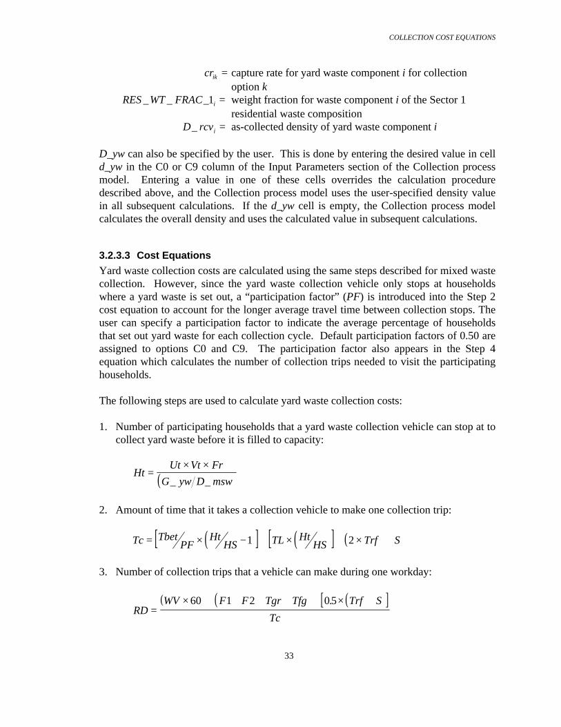
COLLECTION COST EQUATIONS
33
crik = capture rate for yard waste component i for collection option k
RES WT FRAC i_ _ _1 = weight fraction for waste component i of the Sector 1 residential waste composition
D rcvi_ = as-collected density of yard waste component i
D_yw can also be specified by the user. This is done by entering the desired value in celld_yw in the C0 or C9 column of the Input Parameters section of the Collection processmodel. Entering a value in one of these cells overrides the calculation proceduredescribed above, and the Collection process model uses the user-specified density valuein all subsequent calculations. If the d_yw cell is empty, the Collection process modelcalculates the overall density and uses the calculated value in subsequent calculations.
3.2.3.3 Cost Equations
Yard waste collection costs are calculated using the same steps described for mixed wastecollection. However, since the yard waste collection vehicle only stops at householdswhere a yard waste is set out, a “participation factor” (PF) is introduced into the Step 2cost equation to account for the longer average travel time between collection stops. Theuser can specify a participation factor to indicate the average percentage of householdsthat set out yard waste for each collection cycle. Default participation factors of 0.50 areassigned to options C0 and C9. The participation factor also appears in the Step 4equation which calculates the number of collection trips needed to visit the participatinghouseholds.
The following steps are used to calculate yard waste collection costs:
1. Number of participating households that a yard waste collection vehicle can stop at tocollect yard waste before it is filled to capacity:
( )HtUt Vt Fr
G yw D msw=
× ×_ _
2. Amount of time that it takes a collection vehicle to make one collection trip:
( )[ ] ( )[ ] ( )Tc TbetPF
HtHS TL Ht
HS Trf S= × − + × + × +1 2
3. Number of collection trips that a vehicle can make during one workday:
( ) ( ) ( )[ ]
RDWV F F Tgr Tfg Trf S
Tc=
× + + + + + × +60 1 2 0 5.
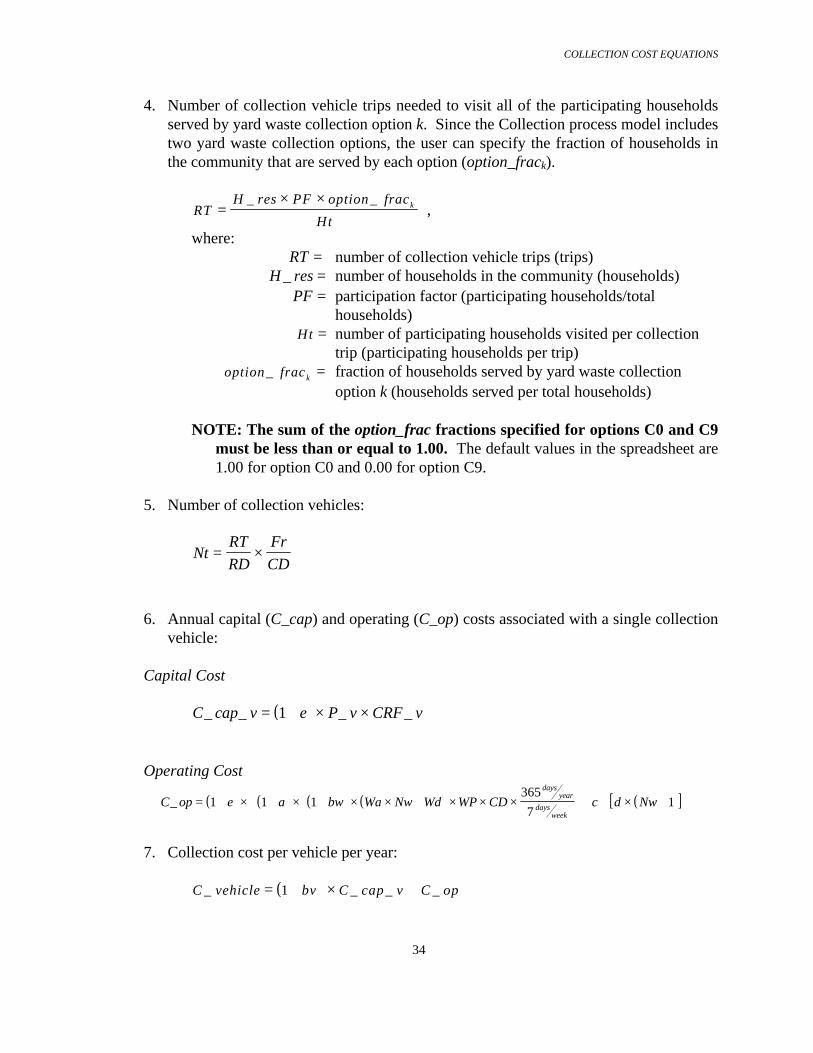
COLLECTION COST EQUATIONS
34
4. Number of collection vehicle trips needed to visit all of the participating householdsserved by yard waste collection option k. Since the Collection process model includestwo yard waste collection options, the user can specify the fraction of households inthe community that are served by each option (option_frack).
RTH res PF option frac
Htk=
× ×_ _ ,
where: RT = number of collection vehicle trips (trips) H res_ = number of households in the community (households)
PF = participation factor (participating households/total households)
Ht = number of participating households visited per collection trip (participating households per trip)
option frac k_ = fraction of households served by yard waste collection option k (households served per total households)
NOTE: The sum of the option_frac fractions specified for options C0 and C9must be less than or equal to 1.00. The default values in the spreadsheet are1.00 for option C0 and 0.00 for option C9.
5. Number of collection vehicles:
NtRTRD
FrCD
= ×
6. Annual capital (C_cap) and operating (C_op) costs associated with a single collection
vehicle: Capital Cost
( )C cap v e P v CRF v_ _ _ _= + × ×1
Operating Cost
( ) ( ) ( ) ( ) ( )[ ]C op e a bw Wa Nw Wd WP CD c d Nwdays
year
daysweek
_ = + × + × + × × + × × ×
+ + × +
1 1 1
365
71
7. Collection cost per vehicle per year:
( )C vehicle bv C cap v C op_ _ _ _= + × +1

COLLECTION COST EQUATIONS
35
8. Annual collection cost for the community:
C ann Nt C vehicle_ _= × 9. Number of participating households that one collection vehicle can visit during a
collection cycle:
H cHt RD CD
Fr_ =
× ×
10. Collection cost per household per year:
C houseC vehicle
H cPF_
_
_= ×
11. Collection cost per ton of yard waste:
C tonC house
G yw PF
lbton
daysweek
daysyear
__
_=
× ×× ×
2000 7
365
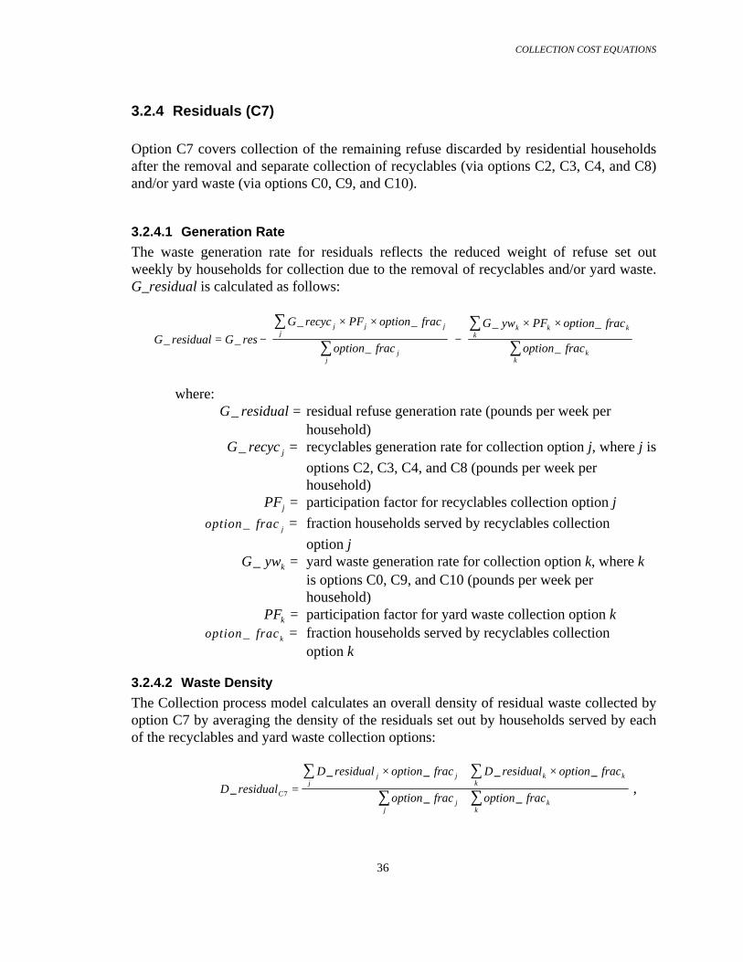
COLLECTION COST EQUATIONS
36
3.2.4 Residuals (C7)
Option C7 covers collection of the remaining refuse discarded by residential householdsafter the removal and separate collection of recyclables (via options C2, C3, C4, and C8)and/or yard waste (via options C0, C9, and C10).
3.2.4.1 Generation Rate
The waste generation rate for residuals reflects the reduced weight of refuse set outweekly by households for collection due to the removal of recyclables and/or yard waste.G_residual is calculated as follows:
G residual G res
G recyc PF option frac
option frac
G yw PF option frac
option frac
j j jj
jj
k k kk
kk
_ _
_ _
_
_ _
_= −
× ×
−
× ×
∑
∑∑
∑
where:G residual_ = residual refuse generation rate (pounds per week per
household) G recyc j_ = recyclables generation rate for collection option j, where j is
options C2, C3, C4, and C8 (pounds per week per household)
PFj = participation factor for recyclables collection option j
option frac j_ = fraction households served by recyclables collection
option j G ywk_ = yard waste generation rate for collection option k, where k
is options C0, C9, and C10 (pounds per week per household)
PFk = participation factor for yard waste collection option k option frac k_ = fraction households served by recyclables collection
option k
3.2.4.2 Waste Density
The Collection process model calculates an overall density of residual waste collected byoption C7 by averaging the density of the residuals set out by households served by eachof the recyclables and yard waste collection options:
D residual
D residual option frac D residual option frac
option frac option fracC
j j k kkj
j kkj
_
_ _ _ _
_ _7 =× + ×
+
∑∑
∑∑ ,
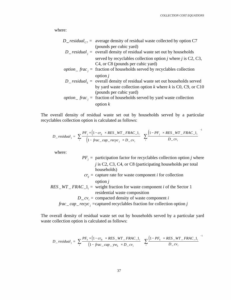
COLLECTION COST EQUATIONS
37
where:
D residualC_ 7 = average density of residual waste collected by option C7 (pounds per cubic yard)
D residual j_ = overall density of residual waste set out by households
served by recyclables collection option j where j is C2, C3, C4, or C8 (pounds per cubic yard)
option frac j_ = fraction of households served by recyclables collection
option j D residualk_ = overall density of residual waste set out households served
by yard waste collection option k where k is C0, C9, or C10(pounds per cubic yard)
option frac j_ = fraction of households served by yard waste collection
option k
The overall density of residual waste set out by households served by a particularrecyclables collection option is calculated as follows:
( )
( )( )
D residualPF cr RES WT FRAC
frac cap recyc D cv
PF RES WT FRAC
D cvj
j ij i
j i
j i
iii
__ _ _
_ _ _
_ _ _
_=
× − ×
− ×+
− ×
∑∑−
1 1
1
1 11
where:PFj = participation factor for recyclables collection option j where
j is C2, C3, C4, or C8 (participating households per total households)
crij = capture rate for waste component i for collection
option j RES WT FRAC i_ _ _1 = weight fraction for waste component i of the Sector 1
residential waste composition D cvi_ = compacted density of waste component i
frac cap recyc j_ _ =captured recyclables fraction for collection option j
The overall density of residual waste set out by households served by a particular yardwaste collection option is calculated as follows:
( )
( )( )
D residualPF cr RES WT FRAC
frac cap yw D cv
PF RES WT FRAC
D cvjk ik i
k i
k i
iii
__ _ _
_ _ _
_ _ _
_=
× − ×
− ×+
− ×
∑∑−
1 1
1
1 11
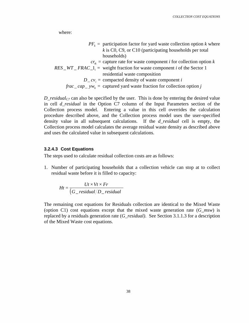
COLLECTION COST EQUATIONS
38
where:
PFk = participation factor for yard waste collection option k wherek is C0, C9, or C10 (participating households per total households)
crik = capture rate for waste component i for collection option k RES WT FRAC i_ _ _1 = weight fraction for waste component i of the Sector 1
residential waste composition D cvi_ = compacted density of waste component i
frac cap ywk_ _ = captured yard waste fraction for collection option j
D_residualC7 can also be specified by the user. This is done by entering the desired valuein cell d_residual in the Option C7 column of the Input Parameters section of theCollection process model. Entering a value in this cell overrides the calculationprocedure described above, and the Collection process model uses the user-specifieddensity value in all subsequent calculations. If the d_residual cell is empty, theCollection process model calculates the average residual waste density as described aboveand uses the calculated value in subsequent calculations.
3.2.4.3 Cost Equations
The steps used to calculate residual collection costs are as follows:
1. Number of participating households that a collection vehicle can stop at to collectresidual waste before it is filled to capacity:
( )HtUt Vt Fr
G residual D residual=
× ×_ _
The remaining cost equations for Residuals collection are identical to the Mixed Waste(option C1) cost equations except that the mixed waste generation rate (G_msw) isreplaced by a residuals generation rate (G_residual). See Section 3.1.1.3 for a descriptionof the Mixed Waste cost equations.

COLLECTION COST EQUATIONS
39
3.2.5 Co-Collection
Co-collection options use a single vehicle to collect mixed waste and recyclables set outby households in different colored bags. The Collection process model includes two co-collection options. The procedures for calculating collection costs for each option arediscussed separately below.
3.2.5.1 Co-Collection Using a Single Compartment Vehicle (C5)
Option C5 covers collection of mixed waste and recyclables bags in a single compartmentvehicle for transport to a transfer station or commingled recyclables MRF. The bags aresorted after they are unloaded at the MRF. Since all of the refuse is collected in a singlecompartment vehicle just as it would be for Mixed Waste Collection (option C1), the costequations for option C5 are identical to the cost equations listed in Section 3.2.1.3 forMixed Waste Collection.
The Input Parameter section of the Collection process model includes a list of defaultcapture rates for each component of the residential waste stream. Although capture ratesare not used to calculate collection cost or life-cycle inventory parameter values, they areincluded in the Collection process model so that they can be accessed by process modelsthat model solid waste treatment and disposal processes.
3.2.5.2 Co-Collection Using a Two Compartment Vehicle (C6)
Option C6 covers collection of bags containing mixed waste and recyclables in separatecompartments of the same vehicle. The vehicle unloads the compartment containingrecyclables bags at a transfer station or commingled recyclables MRF and transports themixed waste bags to a combustion facility, composting facility, landfill, or otherprocessing facility. NOTE: The Collection process model C6 option only includescosts for transporting waste to the initial drop-off point (i.e., transfer station orcommingled recyclables MRF). The cost of subsequent transportation of theremaining bags to another location is included in the cost associated with processingthe refuse at the initial drop-off point.
The Collection process model for option C6 assumes that the two compartments of thecollection vehicle are sized such that they both fill at the same rate. In other words, whenone compartment is filled to capacity and the vehicle stops collecting and travels to itsunloading point, there is no empty space remaining in the other compartment.
3.2.5.2.1 Generation Rates
The value of G_recyc for option C6 is determined using the same procedure as is used tocalculate G_recyc for the recyclables collection options. I.e., the user can specify capture
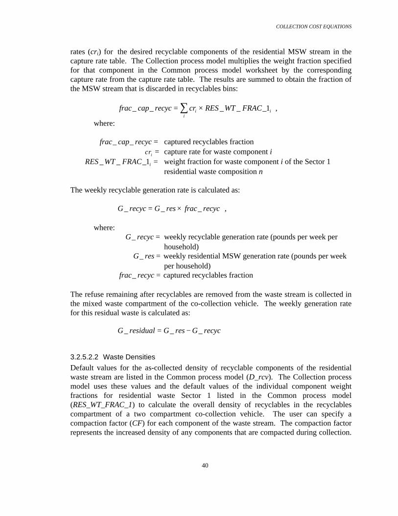
COLLECTION COST EQUATIONS
40
rates (cri) for the desired recyclable components of the residential MSW stream in thecapture rate table. The Collection process model multiplies the weight fraction specifiedfor that component in the Common process model worksheet by the correspondingcapture rate from the capture rate table. The results are summed to obtain the fraction ofthe MSW stream that is discarded in recyclables bins:
frac cap recyc cr RES WT FRACii
i_ _ _ _ _= ×∑ 1 ,
where:
frac cap recyc_ _ = captured recyclables fraction cri = capture rate for waste component i
RES WT FRAC i_ _ _1 = weight fraction for waste component i of the Sector 1residential waste composition n
The weekly recyclable generation rate is calculated as:
G recyc G res frac recyc_ _ _= × ,
where: G recyc_ = weekly recyclable generation rate (pounds per week per
household) G res_ = weekly residential MSW generation rate (pounds per week
per household)frac recyc_ = captured recyclables fraction
The refuse remaining after recyclables are removed from the waste stream is collected inthe mixed waste compartment of the co-collection vehicle. The weekly generation ratefor this residual waste is calculated as:
G residual G res G recyc_ _ _= −
3.2.5.2.2 Waste Densities
Default values for the as-collected density of recyclable components of the residentialwaste stream are listed in the Common process model (D_rcv). The Collection processmodel uses these values and the default values of the individual component weightfractions for residential waste Sector 1 listed in the Common process model(RES_WT_FRAC_1) to calculate the overall density of recyclables in the recyclablescompartment of a two compartment co-collection vehicle. The user can specify acompaction factor (CF) for each component of the waste stream. The compaction factorrepresents the increased density of any components that are compacted during collection.
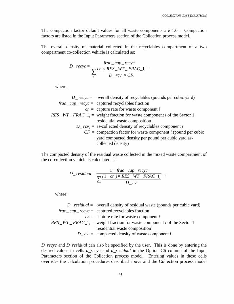
COLLECTION COST EQUATIONS
41
The compaction factor default values for all waste components are 1.0 . Compactionfactors are listed in the Input Parameters section of the Collection process model.
The overall density of material collected in the recyclables compartment of a twocompartment co-collection vehicle is calculated as:
D recycfrac cap recyc
cr RES WT FRACD rcv CF
i i
i ii
__ _
_ _ __
= ××
∑ 1 ,
where:
D recyc_ = overall density of recyclables (pounds per cubic yard) frac cap recyc_ _ = captured recyclables fraction
cri = capture rate for waste component i RES WT FRAC i_ _ _1 = weight fraction for waste component i of the Sector 1
residential waste composition D rcvi_ = as-collected density of recyclables component i
CFi = compaction factor for waste component i (pound per cubicyard compacted density per pound per cubic yard as-collected density)
The compacted density of the residual waste collected in the mixed waste compartment ofthe co-collection vehicle is calculated as:
D residualfrac cap recyc
cr RES WT FRACD cv
i i
ii
__ _
( ) _ _ __
=−
− ×∑1
1 1 ,
where:
D residual_ = overall density of residual waste (pounds per cubic yard) frac cap recyc_ _ = captured recyclables fraction
cri = capture rate for waste component i RES WT FRAC i_ _ _1 = weight fraction for waste component i of the Sector 1
residential waste composition D cvi_ = compacted density of waste component i
D_recyc and D_residual can also be specified by the user. This is done by entering thedesired values in cells d_recyc and d_residual in the Option C6 column of the InputParameters section of the Collection process model. Entering values in these cellsoverrides the calculation procedures described above and the Collection process model
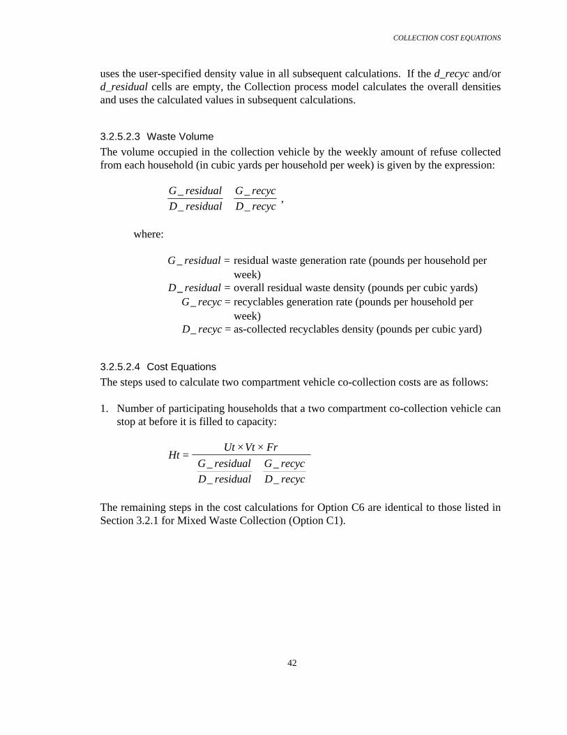
COLLECTION COST EQUATIONS
42
uses the user-specified density value in all subsequent calculations. If the d_recyc and/ord_residual cells are empty, the Collection process model calculates the overall densitiesand uses the calculated values in subsequent calculations.
3.2.5.2.3 Waste Volume
The volume occupied in the collection vehicle by the weekly amount of refuse collectedfrom each household (in cubic yards per household per week) is given by the expression:
G residualD residual
G recycD recyc
__
__
+ ,
where:
G residual_ = residual waste generation rate (pounds per household per week)
D residual_ = overall residual waste density (pounds per cubic yards) G recyc_ = recyclables generation rate (pounds per household per
week) D recyc_ = as-collected recyclables density (pounds per cubic yard)
3.2.5.2.4 Cost Equations
The steps used to calculate two compartment vehicle co-collection costs are as follows:
1. Number of participating households that a two compartment co-collection vehicle canstop at before it is filled to capacity:
HtUt Vt Fr
G residualD residual
G recycD recyc
=× ×
+
__
__
The remaining steps in the cost calculations for Option C6 are identical to those listed inSection 3.2.1 for Mixed Waste Collection (Option C1).

COLLECTION COST EQUATIONS
43
3.2.6 Wet/Dry Collection
Wet/dry collection refers to curbside collection of waste which has been separated byresidents into wet, dry, and recyclable components. The wet and recyclable portions areset out in two separate containers provided by the municipality. Residents provide theirown containers for the dry portion. Collection Option C11 models simultaneouscollection of all three waste types by a three-compartment vehicle. Option C12 modelscollection of the wet and dry portions by a two-compartment vehicle; recyclables arecollected by another vehicle (Option C2, C3, or C4) or taken by residents to a drop-offsite (Option C8). The methods used to calculate waste generation rates, densities, andcollection costs for each option are described below.
3.2.6.1 Wet/Dry/Recyclables (C11)
The user may specify what fraction of each component of MSW will be collected as wetrefuse, dry refuse, and recyclables by making entries in the Wet/Dry/RecyclablesSeparation Factors table located in the Common process model. Component fractions arespecified by entering separation factor values (sf_WDR_weti, sf_WDR_dryi, orsf_WDR_recyci) between 0.00 and 1.00 in the appropriate cells to indicate the fraction ofeach component set out for collection in a wet, dry, or recyclables container. Note: Thewet, dry, and recyclables separation factors for each component of MSW must sumto 1.00. Thus, C11 cannot be used in conjunction with other residential collectionoptions. The components listed below as “Wet” have default sf_WDR_weti values of1.00; components listed as “Dry” have default sf_WDR_dryi values of 1.00. Thecomponents in the list of recyclables have a default sf_WDR_recyci value of 0.75 and adefault sf_WDR_dryi value of 0.25.

COLLECTION COST EQUATIONS
44
WET DRY RECYCLABLES
Leaves Non-recyclable paper Old NewsprintGrass clippings Non-recyclable ferrous metal Old CorrugatedBranches Non-recyclable aluminum CardboardFood waste Non-recyclable glass Office Paper
Non-recyclable plastic Paper - OtherMiscellaneous refuse Ferrous Cans
Ferrous Metal - OtherAluminum CansAluminum - OtherClear GlassBrown GlassGreen GlassTranslucent HDPEPigmented HDPEPETPlastic - Other
3.2.6.1.1 Dry Waste Generation Rate
The dry waste generation rate is the product of dry waste fraction (frac_dry) and theweekly residential waste generation rate:
G dry frac dry G res_ _ _= × ,
where: G dry_ = weekly dry waste generation rate (pounds per week per
household) G res_ = weekly residential waste generation rate (pounds per week
per household)
The dry refuse fraction (frac_dry) is the sum of the weight fractions specified for eachcomponent in the Sector 1 residential waste composition list in the Common processmodel multiplied by the corresponding dry refuse separation factor:
frac dry RES WT FRAC sf WDR dryi ii
_ _ _ _ _ _= ×∑ 1 ,
where:
frac dry_ = dry refuse fraction RES WT FRAC i_ _ _1 = weight fraction for waste component i of
the Sector 1 residential waste composition

COLLECTION COST EQUATIONS
45
sf WDR dryi_ _ = dry refuse separation factor for waste component i
3.2.6.1.2 Wet Waste Generation Rate
The wet waste generation rate is the product of the wet waste fraction (frac_wet) and thetotal weekly refuse generation rate (G_res):
G wet frac wet G res_ _ _= ×
where: G wet_ = weekly wet waste generation rate (pounds per week
per household)
The wet refuse fraction (frac_wet) is the sum of the weight fractions specified for eachcomponents in the Sector 1 residential waste composition list in the Common processmodel multiplied by the corresponding wet refuse separation factor:
frac wet RES WT FRAC sf WDR weti ii
_ _ _ _ _ _= ×∑ 1 ,
where:
frac wet_ = wet refuse fraction RES WT FRAC i_ _ _1 = weight fraction for waste component i of
the Sector 1 residential waste composition sf WDR weti_ _ = wet refuse separation factor for waste component i
3.2.6.1.3 Recyclables Generation Rate
The recyclables generation rate is the product of the captured recyclables fraction(frac_cap_recyc) and the total weekly refuse generation rate (G_res):
G recyc frac cap recyc G res_ _ _ _= × ,
where: G recyc_ = weekly recyclables waste generation rate (pounds
per week per household)
The captured recyclables fraction (frac_cap_recyc) is the sum of the weight fractionsspecified for each component in the Sector 1 residential waste composition list in theCommon process model (RES_WT_FRAC_1) multiplied by the recyclables separationfactor specified for that component in the Common process model:
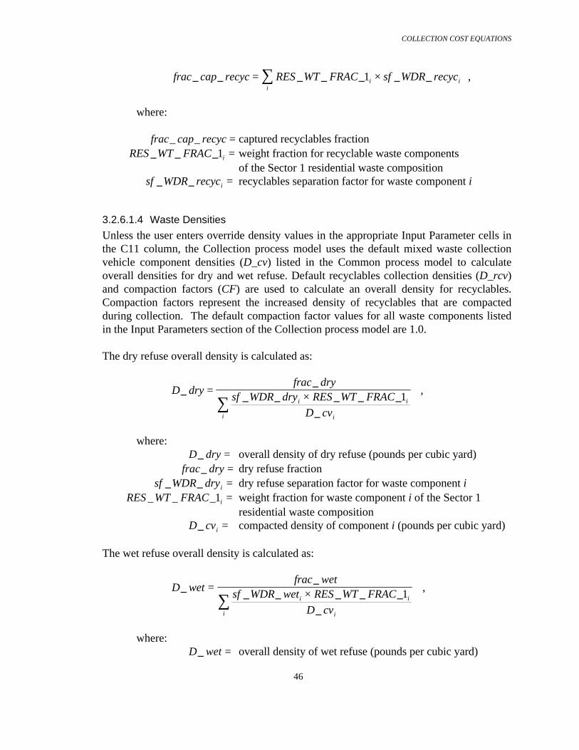
COLLECTION COST EQUATIONS
46
frac cap recyc RES WT FRAC sf WDR recyci ii
_ _ _ _ _ _ _= ×∑ 1 ,
where:
frac cap recyc_ _ = captured recyclables fraction RES WT FRAC i_ _ _1 = weight fraction for recyclable waste components
of the Sector 1 residential waste composition sf WDR recyci_ _ = recyclables separation factor for waste component i
3.2.6.1.4 Waste Densities
Unless the user enters override density values in the appropriate Input Parameter cells inthe C11 column, the Collection process model uses the default mixed waste collectionvehicle component densities (D_cv) listed in the Common process model to calculateoverall densities for dry and wet refuse. Default recyclables collection densities (D_rcv)and compaction factors (CF) are used to calculate an overall density for recyclables.Compaction factors represent the increased density of recyclables that are compactedduring collection. The default compaction factor values for all waste components listedin the Input Parameters section of the Collection process model are 1.0.
The dry refuse overall density is calculated as:
D dryfrac dry
sf WDR dry RES WT FRACD cv
i i
ii
__
_ _ _ _ __
= ×∑ 1 ,
where: D dry_ = overall density of dry refuse (pounds per cubic yard) frac dry_ = dry refuse fraction
sf WDR dryi_ _ = dry refuse separation factor for waste component i RES WT FRAC i_ _ _1 = weight fraction for waste component i of the Sector 1
residential waste composition D cvi_ = compacted density of component i (pounds per cubic yard)
The wet refuse overall density is calculated as:
D wetfrac wet
sf WDR wet RES WT FRACD cv
i i
ii
__
_ _ _ _ __
= ×∑ 1 ,
where: D wet_ = overall density of wet refuse (pounds per cubic yard)
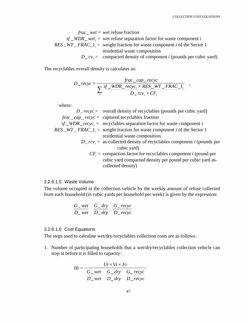
COLLECTION COST EQUATIONS
47
frac wet_ = wet refuse fraction sf WDR weti_ _ = wet refuse separation factor for waste component i
RES WT FRAC i_ _ _1 = weight fraction for waste component i of the Sector 1 residential waste composition
D cvi_ = compacted density of component i (pounds per cubic yard)
The recyclables overall density is calculates as:
D recycfrac cap recyc
sf WDR recyc RES WT FRACD rcv CF
i i
i ii
__ _
_ _ _ _ _
_
= ××
∑ 1 ,
where: D recyc_ = overall density of recyclables (pounds per cubic yard)
frac cap recyc_ _ = captured recyclables fraction sf WDR recyci_ _ = recyclables separation factor for waste component i
RES WT FRAC i_ _ _1 = weight fraction for waste component i of the Sector 1 residential waste composition
D rcvi_ = as-collected density of recyclables component i (pounds percubic yard)
CFi = compaction factor for recyclables component i (pound per cubic yard compacted density per pound per cubic yard as-collected density)
3.2.6.1.5 Waste Volume
The volume occupied in the collection vehicle by the weekly amount of refuse collectedfrom each household (in cubic yards per household per week) is given by the expression:
G wetD wet
G dryD dry
G recycD recyc
_
_
_
_
_
_+ +
3.2.6.1.6 Cost Equations
The steps used to calculate wet/dry/recyclables collection costs are as follows:
1. Number of participating households that a wet/dry/recyclables collection vehicle canstop at before it is filled to capacity:
HtUt Vt Fr
G wetD wet
G dryD dry
G recycD recyc
=× ×
+ +
__
__
__
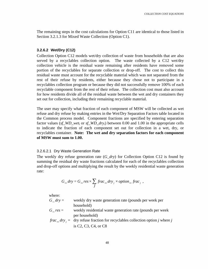
COLLECTION COST EQUATIONS
48
The remaining steps in the cost calculations for Option C11 are identical to those listed inSection 3.2.1.3 for Mixed Waste Collection (Option C1).
3.2.6.2 Wet/Dry (C12)
Collection Option C12 models wet/dry collection of waste from households that are alsoserved by a recyclables collection option. The waste collected by a C12 wet/drycollection vehicle is the residual waste remaining after residents have removed someportion of the recyclables for separate collection or drop-off. The cost to collect thisresidual waste must account for the recyclable material which was not separated from therest of their refuse by residents, either because they chose not to participate in arecyclables collection program or because they did not successfully remove 100% of eachrecyclable component from the rest of their refuse. The collection cost must also accountfor how residents divide all of the residual waste between the wet and dry containers theyset out for collection, including their remaining recyclable material.
The user may specify what fraction of each component of MSW will be collected as wetrefuse and dry refuse by making entries in the Wet/Dry Separation Factors table located inthe Common process model. Component fractions are specified by entering separationfactor values (sf_WD_weti or sf_WD_dryi) between 0.00 and 1.00 in the appropriate cellsto indicate the fraction of each component set out for collection in a wet, dry, orrecyclables container. Note: The wet and dry separation factors for each componentof MSW must sum to 1.00.
3.2.6.2.1 Dry Waste Generation Rate
The weekly dry refuse generation rate (G_dry) for Collection Option C12 is found bysumming the residual dry waste fractions calculated for each of the recyclables collectionand drop-off options and multiplying the result by the weekly residential waste generationrate:
G dry G res frac dry option fracj
j j_ _ _ _= × ×∑ ,
where:G dry_ = weekly dry waste generation rate (pounds per week per
household)G res_ = weekly residential waste generation rate (pounds per week
per household)frac dry j_ = dry refuse fraction for recyclables collection option j where j
is C2, C3, C4, or C8

COLLECTION COST EQUATIONS
49
option frac j_ = fraction of households served by recyclables collection
option j
The dry residuals fraction for a particular recyclables collection option (frac_dryj) is thesum of the dry portion of the remaining recyclables components from participating andnon-participating households plus the dry portion of the non-recyclables components.This can be calculated as:
( ) ( )[ ]frac dry RES WT FRAC sf WDR dry PF cr PFj i i j ij ji
_ _ _ _ _ _= × × × − + −∑ 1 1 1 ,
where:
frac dry j_ = dry refuse fraction for recyclables collection option j
RES WT FRAC i_ _ _1 = weight fraction for waste component i of the Sector 1 residential waste composition
sf WDR dryi_ _ = dry refuse separation factor for waste component iPFj = participation factor for recyclables collection option j
crij = capture rate for component i, recyclables collection option j
3.2.6.2.2 Wet Waste Generation Rate
The weekly wet refuse generation rate (G_wet) for Collection Option C12 is found bysumming the residual wet waste fractions calculated for each of the recyclables collectionand drop-off options and multiplying the result by the weekly residential waste generationrate:
G wet G res frac wet option fracj
j j_ _ _ _= × ×∑ ,
where: G wet_ = weekly wet waste generation rate (pounds per week per
household) G res_ = weekly residential waste generation rate (pounds per week
per household) frac wet j_ = wet refuse fraction for recyclables collection option j where
j is C2, C3, C4, or C8 option frac j_ = fraction of households served by recyclables collection
option j
The wet residuals fraction for a particular recyclables collection option (frac_wetj) is thesum of the wet portion of the remaining recyclables components from participating and

COLLECTION COST EQUATIONS
50
non-participating households plus the wet portion of the non-recyclables components.This can be calculated as:
( ) ( )[ ]frac wet RES WT FRAC sf WDR wet PF cr PFj i i j ij ji
_ _ _ _ _ _= × × × − + −∑ 1 1 1 ,
where:
frac wet j_ = wet refuse fraction for recyclables collection option j
RES WT FRAC i_ _ _1 = weight fraction for waste component i of the Sector 1 residential waste composition
sf WDR weti_ _ = wet refuse separation factor for waste component iPFj = participation factor for recyclables collection option j
crij = capture rate for component i, recyclables collection option j
3.2.6.2.3 Wet Waste Density
Unless the user enters an override wet waste density in the d_wet cell in the C12 column,the Collection process model calculates the overall wet waste density by averaging theoverall wet densities of residual waste collected from households served by differentrecyclables collection options:
D wet D wet option fracC j jj
_ _ _12 = ×∑ ,
where: D wetC_ 12 = overall density of wet refuse collected by a C12 wet/dry
collection vehicle (pounds per cubic yard) D wet j_ = overall density of wet refuse from households served by
recyclables collection option j, where j is C2, C3, C4, or C8 option frac j_ = fraction of households served by collection option j
The overall wet density of waste collected from households that are served by a particularrecyclables collection option (D_wetj) must account for both the wet portions of the non-recyclable components of the waste stream and the wet portions of the recyclablecomponents which were not collected from participating and non-participatinghouseholds. D_wetj is calculated as:
( ) ( )[ ]D wet
frac wet
sf WDR wet RES WT FRAC PF cr PF
D cv
j
j
i i j ij j
ii
__
_ _ _ _ _
_
=× × × − + −
∑1 1 1

COLLECTION COST EQUATIONS
51
where: D wet j_ = overall density of wet waste from households served by
recyclables collection option j (pounds per cubic yard) frac wet j_ = wet refuse fraction for recyclables collection option j
sf WDR weti_ _ = wet refuse separation factor for waste component i RES WT FRAC i_ _ _1 = weight fraction for waste component i of the Sector 1
residential waste compositionPFj = participation factor for recyclables collection option j
crij = capture rate for component i, recyclables collection option j
D cvi_ = compacted density of component i (pounds per cubic yard)
3.2.6.2.4 Dry Waste Density
Unless the user enters an override dry waste density in the d_dry cell in the C12 column,the Collection process model calculates the overall dry waste density by averaging theoverall dry densities of residual waste collected from households served by differentrecyclables collection options:
D dry D dry option fracC j jj
_ _ _12 = ×∑
where: D dryC_ 12 = overall density of dry refuse collected by a C12 wet/dry
collection vehicle (pounds per cubic yard) D dry j_ = overall density of dry refuse from households served by
recyclables collection option j, where j is C2, C3, C4, or C8 option frac j_ = fraction of households served by collection option j
The overall dry density of waste collected from households that are served by a particularrecyclables collection option (D_dryj) must account for both the dry portions of the non-recyclable components of the waste stream and the dry portions of the recyclablecomponents which were not collected from participating and non-participatinghouseholds. D_dryj is calculated as:
( ) ( )[ ]D dryfrac dry
sf WDR dry RES WT FRAC PF cr PF
D cv
j
j
i i j ij j
ii
__
_ _ _ _ _
_
=× × × − + −
∑1 1 1
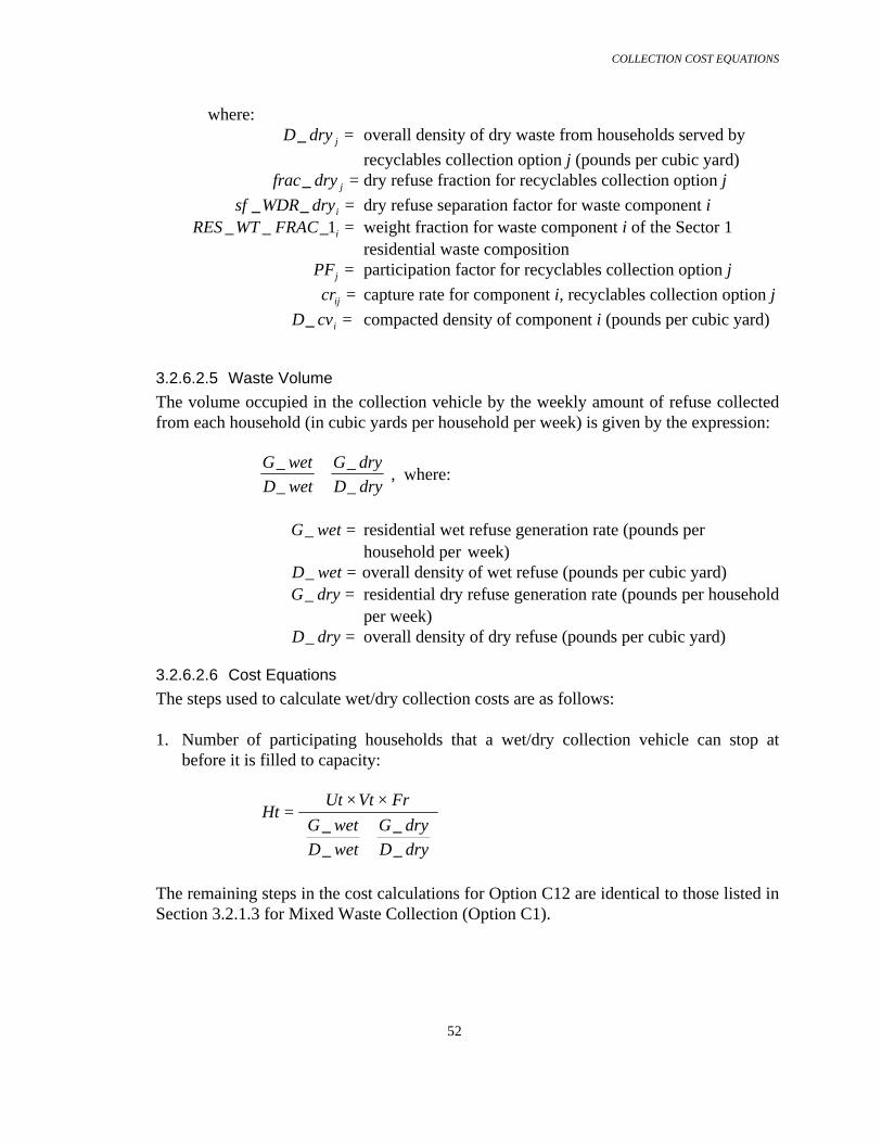
COLLECTION COST EQUATIONS
52
where: D dry j_ = overall density of dry waste from households served by
recyclables collection option j (pounds per cubic yard) frac dry j_ = dry refuse fraction for recyclables collection option j
sf WDR dryi_ _ = dry refuse separation factor for waste component i RES WT FRAC i_ _ _1 = weight fraction for waste component i of the Sector 1
residential waste compositionPFj = participation factor for recyclables collection option j
crij = capture rate for component i, recyclables collection option j
D cvi_ = compacted density of component i (pounds per cubic yard)
3.2.6.2.5 Waste Volume
The volume occupied in the collection vehicle by the weekly amount of refuse collectedfrom each household (in cubic yards per household per week) is given by the expression:
G wetD wet
G dryD dry
_
_
_
_+ , where:
G wet_ = residential wet refuse generation rate (pounds per household per week)
D wet_ = overall density of wet refuse (pounds per cubic yard) G dry_ = residential dry refuse generation rate (pounds per household
per week) D dry_ = overall density of dry refuse (pounds per cubic yard)
3.2.6.2.6 Cost Equations
The steps used to calculate wet/dry collection costs are as follows:
1. Number of participating households that a wet/dry collection vehicle can stop atbefore it is filled to capacity:
HtUt Vt Fr
G wetD wet
G dryD dry
=× ×
+
__
__
The remaining steps in the cost calculations for Option C12 are identical to those listed inSection 3.2.1.3 for Mixed Waste Collection (Option C1).

COLLECTION COST EQUATIONS
53
3.3 Residential Waste Drop-Off
The Collection process model includes two collection options that model drop-off ofselected components of residential MSW at a drop-off site by residents using their ownvehicles. For Option C8 (Recyclables Drop-Off) the drop-off site consists of roll-on/roll-off containers at a central location in the community. Municipal collection vehiclesperiodically transport full containers to a disposal facility. For Option C10 (Yard WasteDrop-Off) participating households transport their yard waste directly to a disposalfacility for composting or some other waste disposal process.

COLLECTION COST EQUATIONS
54
3.3.1 Recyclables (C8)
Option C8 models transport of recyclables by residents using their own vehicles to acentrally located drop-off site. Residents deposit recyclables in roll-on/roll-off containersat the drop-off site. Municipal collection vehicles are dispatched from a garage at thebeginning of a workday to off-load empty containers at the drop-off site and on-load fullcontainers. Full containers are taken to a recycling facility (a MRF, for example) andemptied. Collection vehicles then return to the drop-off site and repeat the process untilthe end of the workday when they return to the vehicle garage. Only the capital andoperating costs associated with the municipal collection vehicles are included in theOption C8 cost calculations; costs associated with the drop-off vehicles used by residentsare excluded. However, life-cycles parameters for both collection vehicles and drop-offvehicles are accounted for as described in Sections 5-8.
3.3.1.1 Generation Rate
The weekly generation rate for recyclables (G_recyc) is a function of the weekly MSWgeneration rate (G_res) and the amount of recyclables removed from the waste stream.The user can specify values for these variables by entering values in the appropriate cellsin the Collection process model worksheet to override the process model default values.
The captured recyclables fraction (frac_cap_recyc) is found by summing the fraction ofrecyclable material removed by households from each component of the residential MSWstream. A table is provided in the Collection process model worksheet where the user canenter values to identify what fraction on average of each recyclable component isremoved by participating households from their mixed waste for transport and disposal atthe drop-off site. This fraction is referred to as the “capture rate” (cr). Entering a valueof 0.75 as the capture rate for aluminum cans, for instance, indicates that on averagehouseholds successfully remove 75% of their aluminum cans from their refuse. The other25% is collected along with other non-captured recyclables and the household’s non-recyclable refuse by another collection vehicle. Costs for collection of this “residual”waste are accounted for by one of the residuals collection options (C7 or C12). Leaving acell blank or entering a zero in the capture rate table indicates that the componentrepresented by that cell is not included in the recyclables drop-off program.
Default capture rates are assigned to the following residential waste stream components:
• Old Newsprint• Old Corrugated Cardboard• Office Paper• Paper Other (5 classes)• Ferrous Cans
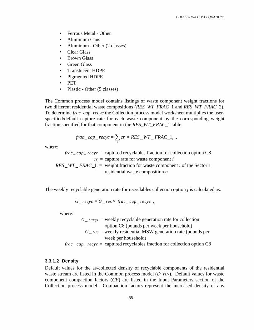
COLLECTION COST EQUATIONS
55
• Ferrous Metal - Other• Aluminum Cans• Aluminum - Other (2 classes)• Clear Glass• Brown Glass• Green Glass• Translucent HDPE• Pigmented HDPE• PET• Plastic - Other (5 classes)
The Common process model contains listings of waste component weight fractions fortwo different residential waste compositions (RES_WT_FRAC_1 and RES_WT_FRAC_2).To determine frac_cap_recyc the Collection process model worksheet multiplies the user-specified/default capture rate for each waste component by the corresponding weightfraction specified for that component in the RES_WT_FRAC_1 table:
frac cap recyc cr RES WT FRACii
i_ _ _ _ _= ×∑ 1 ,
where: frac cap recyc_ _ = captured recyclables fraction for collection option C8
cri = capture rate for waste component i RES WT FRAC i_ _ _1 = weight fraction for waste component i of the Sector 1
residential waste composition n
The weekly recyclable generation rate for recyclables collection option j is calculated as:
G recyc G res frac cap recyc_ _ _ _= × ,
where: G recyc_ = weekly recyclable generation rate for collection
option C8 (pounds per week per household) G res_ = weekly residential MSW generation rate (pounds per
week per household) frac cap recyc_ _ = captured recyclables fraction for collection option C8
3.3.1.2 Density
Default values for the as-collected density of recyclable components of the residentialwaste stream are listed in the Common process model (D_rcv). Default values for wastecomponent compaction factors (CF) are listed in the Input Parameters section of theCollection process model. Compaction factors represent the increased density of any

COLLECTION COST EQUATIONS
56
waste components that are compacted during collection from the drop-off site. Thedefault compaction factor values for all waste components are 1.0 . The Collectionprocess model uses these values and the default values of the individual componentweight fractions for residential waste Sector 1 listed in the Common process model(RES_WT_FRAC_1) to calculate an overall density for residential recyclables in arecyclables collection vehicle.
D recycfrac cap recyc
cr RES WT FRACD rcv CF
i i
i ii
__ _
_ _ _
_
= ××
∑ 1 ,
where:
D recyc_ = overall density of recyclables (pounds per cubic yard) frac cap recyc_ _ = captured recyclables fraction
cri = capture rate for waste component i RES WT FRAC i_ _ _1 = weight fraction for waste component i of the Sector 1
residential waste composition D rcvi_ = as-collected density of recyclables component i
CFi = compaction factor for waste component i (pound per cubic yard compacted density per pound per cubic yard as-collected density)
D_recyc can also be specified by the user. This is done by entering the desired value incell d_recyc in the Option C8 column of the Input Parameters section of the Collectionprocess model. Entering a value in this cell overrides the calculation procedure describedabove. The Collection process model uses the user-specified density value in allsubsequent calculations. If the d_recyc cell is empty, the Collection process modelcalculates the overall density and uses the calculated value in subsequent calculations.
3.3.1.3 Cost Equations
Option C8 costs are calculated using the following steps:
1. Volume of recyclables that accumulate at the drop-off site per week:
vol recycH res PF G recyc
D recyc_
_ _
_=
× × ,
where: vol recyc_ = weekly volume of recyclables deposited at drop-off site
(cubic yards per week) H res_ = number of households in the community (households)
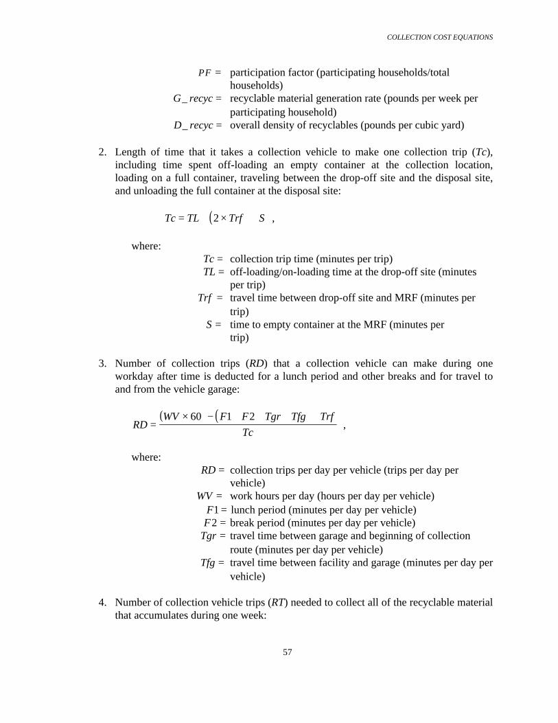
COLLECTION COST EQUATIONS
57
PF = participation factor (participating households/total households)
G recyc_ = recyclable material generation rate (pounds per week per participating household)
D recyc_ = overall density of recyclables (pounds per cubic yard) 2. Length of time that it takes a collection vehicle to make one collection trip (Tc),
including time spent off-loading an empty container at the collection location,loading on a full container, traveling between the drop-off site and the disposal site,and unloading the full container at the disposal site:
( )Tc TL Trf S= + × +2 , where:
Tc = collection trip time (minutes per trip) TL = off-loading/on-loading time at the drop-off site (minutes per trip) Trf = travel time between drop-off site and MRF (minutes per
trip) S = time to empty container at the MRF (minutes per
trip) 3. Number of collection trips (RD) that a collection vehicle can make during one
workday after time is deducted for a lunch period and other breaks and for travel toand from the vehicle garage:
( ) ( )
RDWV F F Tgr Tfg Trf
Tc=
× − + + + +60 1 2 ,
where:
RD = collection trips per day per vehicle (trips per day per vehicle)
WV = work hours per day (hours per day per vehicle) F1 = lunch period (minutes per day per vehicle) F2 = break period (minutes per day per vehicle) Tgr = travel time between garage and beginning of collection
route (minutes per day per vehicle) Tfg = travel time between facility and garage (minutes per day per
vehicle) 4. Number of collection vehicle trips (RT) needed to collect all of the recyclable material
that accumulates during one week:

COLLECTION COST EQUATIONS
58
RTvol recycVc Uc
=×
_ ,
where:
RT = number of collection vehicle trips per week (trips per week) Vc = roll-on/roll-off container capacity (cubic yards per trip) Uc = roll-on/roll-off container utilization factor (%)
5. Number of collection vehicles needed collect all of the accumulated recyclable
material:
NtRT
RD CD=
× ,
where:
Nt = number of collection vehicles (vehicles) CD = number of workdays per week (days per week)
6. Annual capital (C_cap) and operating (C_op) costs associated with a single collectionvehicle:
Capital Cost
( )C cap v e Pt CRF_ _ = + × ×1
Operating Cost
( ) ( ) ( ) ( ) ( )[ ]C e a bw Wa Nw Wd WP CD c d Nwopdays
year
daysweek
_ = + × + × + × × + × × ×
+ + × +
1 1 1
365
71
7. Collection cost per vehicle per year:
( )C vehicle bv C cap v C cap b C op_ _ _ _ _ _= + × + +1 8. Total annual collection cost (C_ann) for the community:
C ann Nt C vehicle_ _= ×
9. Collection cost per household per year:
( )C houseC vehicle PF
RD CD Ut Vt D recyc G recyc_
_
_ _=
×× × × ×

COLLECTION COST EQUATIONS
59
10. Collection cost per ton of recyclables:
C tonC house
G recyc PF
lbton
daysweek
daysyear
__
_=
× ×× ×2000 7
365
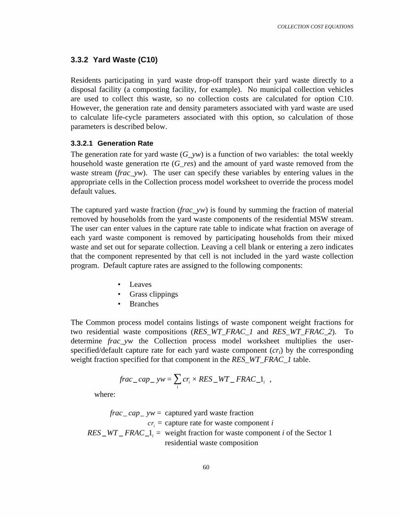
COLLECTION COST EQUATIONS
60
3.3.2 Yard Waste (C10)
Residents participating in yard waste drop-off transport their yard waste directly to adisposal facility (a composting facility, for example). No municipal collection vehiclesare used to collect this waste, so no collection costs are calculated for option C10.However, the generation rate and density parameters associated with yard waste are usedto calculate life-cycle parameters associated with this option, so calculation of thoseparameters is described below.
3.3.2.1 Generation Rate
The generation rate for yard waste (G_yw) is a function of two variables: the total weeklyhousehold waste generation rte (G_res) and the amount of yard waste removed from thewaste stream (frac_yw). The user can specify these variables by entering values in theappropriate cells in the Collection process model worksheet to override the process modeldefault values.
The captured yard waste fraction (frac_yw) is found by summing the fraction of materialremoved by households from the yard waste components of the residential MSW stream.The user can enter values in the capture rate table to indicate what fraction on average ofeach yard waste component is removed by participating households from their mixedwaste and set out for separate collection. Leaving a cell blank or entering a zero indicatesthat the component represented by that cell is not included in the yard waste collectionprogram. Default capture rates are assigned to the following components:
• Leaves• Grass clippings• Branches
The Common process model contains listings of waste component weight fractions fortwo residential waste compositions (RES_WT_FRAC_1 and RES_WT_FRAC_2). Todetermine frac_yw the Collection process model worksheet multiplies the user-specified/default capture rate for each yard waste component (cri) by the correspondingweight fraction specified for that component in the RES_WT_FRAC_1 table.
frac cap yw cr RES WT FRACii
i_ _ _ _ _= ×∑ 1 ,
where:
frac cap yw_ _ = captured yard waste fraction cri = capture rate for waste component i
RES WT FRAC i_ _ _1 = weight fraction for waste component i of the Sector 1residential waste composition

COLLECTION COST EQUATIONS
61
The weekly recyclable generation rate for yard waste is calculated as:
G yw G res frac cap yw_ _ _ _= × ,
where: G yw_ = weekly yard waste generation rate (pounds per
week per participating household) G res_ = weekly residential MSW generation rate (pounds
per week per participating household) frac cap yw_ _ = captured yard waste fraction
3.3.2.2 Density
Default values for the as-collected density of yard waste components of the residentialwaste stream are listed in the Common process model (D_rcv). The Collection processmodel uses these values and the default values of the individual component weightfractions for residential waste Sector 1 listed in the Common process model(RES_WT_FRAC_1) to calculate an overall density for residential yard waste in acollection vehicle:
D ywfrac cap yw
cr RES WT FRACD rcv
i i
ii
__ __ _ _
_
= ×∑ 1 ,
where:
D yw_ = overall density of yard waste (pounds per cubic yard) frac cap yw_ _ = captured yard waste fraction
cri = capture rate for yard waste component i RES WT FRAC i_ _ _1 = weight fraction for waste component i of the Sector 1
residential waste composition D rcvi_ = as-collected density of yard waste component i
D_yw can also be specified by the user. This is done by entering the desired value in celld_yw in the C10 column of the Input Parameters section of the Collection process model.Entering a value in this cell overrides the calculation procedure described above, and theCollection process model uses the user-specified density value in all subsequentcalculations. If the d_yw cell is empty, the Collection process model calculates theoverall density and uses the calculated value in subsequent calculations.
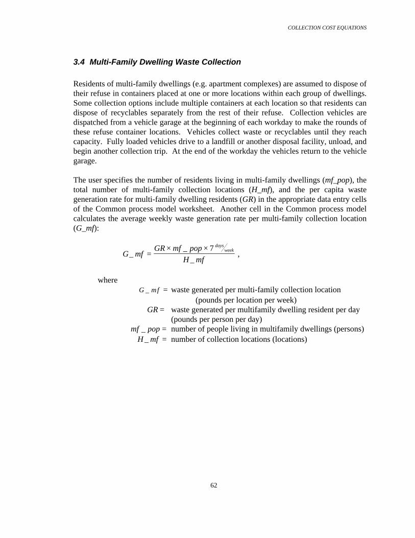
COLLECTION COST EQUATIONS
62
3.4 Multi-Family Dwelling Waste Collection
Residents of multi-family dwellings (e.g. apartment complexes) are assumed to dispose oftheir refuse in containers placed at one or more locations within each group of dwellings.Some collection options include multiple containers at each location so that residents candispose of recyclables separately from the rest of their refuse. Collection vehicles aredispatched from a vehicle garage at the beginning of each workday to make the rounds ofthese refuse container locations. Vehicles collect waste or recyclables until they reachcapacity. Fully loaded vehicles drive to a landfill or another disposal facility, unload, andbegin another collection trip. At the end of the workday the vehicles return to the vehiclegarage.
The user specifies the number of residents living in multi-family dwellings (mf_pop), thetotal number of multi-family collection locations (H_mf), and the per capita wastegeneration rate for multi-family dwelling residents (GR) in the appropriate data entry cellsof the Common process model worksheet. Another cell in the Common process modelcalculates the average weekly waste generation rate per multi-family collection location(G_mf):
G mfGR mf pop
H mf
daysweek
__
_=
× × 7 ,
where G mf_ = waste generated per multi-family collection location
(pounds per location per week) GR = waste generated per multifamily dwelling resident per day
(pounds per person per day) mf pop_ = number of people living in multifamily dwellings (persons) H mf_ = number of collection locations (locations)

COLLECTION COST EQUATIONS
63
3.4.1 Mixed Waste (C13)
Collection option C13 models collection of multi-family waste using single compartmentcollection vehicles. There is no separation of the waste at the point of collection, eitherby residents or the collection vehicle crews. The collection vehicles transport the wasteto a treatment or disposal facility such as a landfill, MRF, of transfer station.
3.4.1.1 Generation Rate
Since there is no waste separation at the point of collection for this collection option, theweekly mixed waste generation rate (G_msw) at multi-family collection locations is thesame as the weekly multi-family waste generation rate calculated by the Common processmodel:
G msw G mf_ _=
3.4.1.2 Waste Density
Default values for the compacted density of individual components of the waste streamare listed in the Collection process model (D_cv). The Collection process model usesthese values and the default values of the individual component weight fractions formulti-family waste sector 1 listed in the Common process model (RES_WT_FRAC_1) tocalculate an overall density for multi-family mixed waste:
D mswMF WT FRAC
D cvi
ii
__ _ _
_
=∑
11
,
where:
D msw_ = overall density of mixed waste (pounds per cubic yard) MF WT FRAC i_ _ _1 = weight fraction for waste component i of the Sector 1
multi-family waste composition D cvi_ = compacted density of waste component I (pounds per
cubic yard)
This value represents the overall density of the waste after compaction in the collectionvehicle.
D_msw can also be specified by the user. This is done by entering the desired value incell d_msw in the Option C13 column of the Input Parameters section of the Collectionprocess model. Entering a value in this cell overrides the calculation procedure described
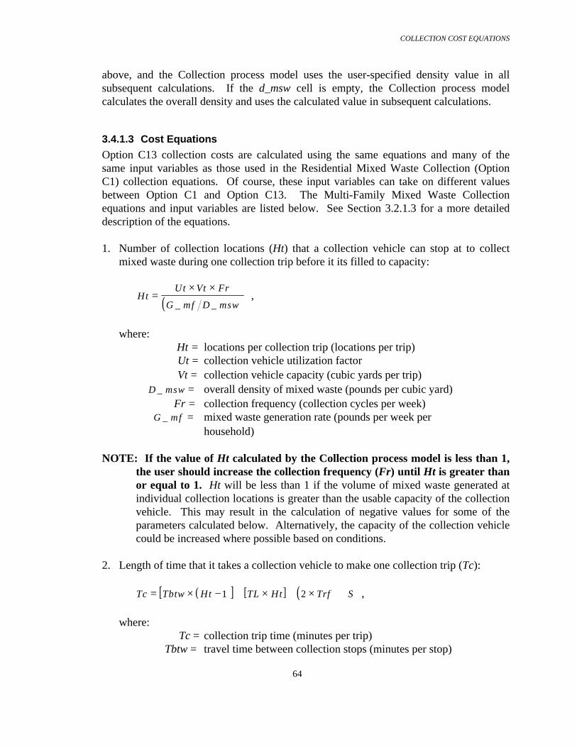
COLLECTION COST EQUATIONS
64
above, and the Collection process model uses the user-specified density value in allsubsequent calculations. If the d_msw cell is empty, the Collection process modelcalculates the overall density and uses the calculated value in subsequent calculations.
3.4.1.3 Cost Equations
Option C13 collection costs are calculated using the same equations and many of thesame input variables as those used in the Residential Mixed Waste Collection (OptionC1) collection equations. Of course, these input variables can take on different valuesbetween Option C1 and Option C13. The Multi-Family Mixed Waste Collectionequations and input variables are listed below. See Section 3.2.1.3 for a more detaileddescription of the equations.
1. Number of collection locations (Ht) that a collection vehicle can stop at to collectmixed waste during one collection trip before it its filled to capacity:
( )HtUt Vt Fr
G mf D msw=
× ×_ _
,
where: Ht = locations per collection trip (locations per trip) Ut = collection vehicle utilization factor Vt = collection vehicle capacity (cubic yards per trip) D msw_ = overall density of mixed waste (pounds per cubic yard) Fr = collection frequency (collection cycles per week) G mf_ = mixed waste generation rate (pounds per week per
household)
NOTE: If the value of Ht calculated by the Collection process model is less than 1,the user should increase the collection frequency (Fr) until Ht is greater thanor equal to 1. Ht will be less than 1 if the volume of mixed waste generated atindividual collection locations is greater than the usable capacity of the collectionvehicle. This may result in the calculation of negative values for some of theparameters calculated below. Alternatively, the capacity of the collection vehiclecould be increased where possible based on conditions.
2. Length of time that it takes a collection vehicle to make one collection trip (Tc):
( )[ ] [ ] ( )Tc Tbtw Ht TL Ht Trf S= × − + × + × +1 2 , where: Tc = collection trip time (minutes per trip) Tbtw = travel time between collection stops (minutes per stop)

COLLECTION COST EQUATIONS
65
TL = loading time at a collection stop (minutes per stop) Trf = travel time between beginning/end of collection route and
disposal facility (minutes) S = time to unload collection vehicle at the disposal facility
(minutes) 3. Number of collection trips that a vehicle can make during one workday after time is
deducted for a lunch period and other breaks and for travel to and from the vehiclegarage:
( ) ( ) ( )[ ]
RDWV F F Tgr Tfg Trf S
Tc=
× + + + + + × +60 1 2 0 5. ,
where: RD = collection trips per day per vehicle (trips per day per
vehicle) WV = work hours per day (hours per day per vehicle) F1 = lunch period (minutes per day per vehicle) F2 = break period (minutes per day per vehicle) Tgr = travel time between garage and beginning of collection
route (minutes) Tfg = travel time between facility and garage (minutes) 4. Number of collection vehicle trips (RT) needed to visit all of the multi-family
collection locations in the community served by collection option C13:
RTH mf option frac
Ht=
×_ _ ,
where: RT = number of collection trips (trips) option frac_ = fraction of collection locations served by collection option C13 5. Number of collection vehicles (Nt) needed to visit all of the multi-family collection
locations in the community served by collection option C13 during one collectioncycle:
NtRT
RD
Fr
CD= × ,
where: Nt = number of collection vehicles (vehicles) CD = number of workdays per week (days per week)

COLLECTION COST EQUATIONS
66
6. Annual capital (C_cap) and operating (C_op) costs associated with a single collection
vehicle: Capital Cost ( )C cap e Pt CRF_ = + × ×1 , where: C cap_ = collection vehicle capital cost amortized over the economic
life of the vehicle ($ per vehicle per year) e = administrative rate ($ of administrative expense per $ of
capital cost or operating expense) Pt = unit price of a collection vehicle ($ per vehicle) CRF = capital recovery factor for a vehicle (year-1)
The capital recovery factor is defined as:
( )( )
CRFi i
i
L
L=× ++ −
1
1 1 ,
where: i = yearly discount rate (year-1) L = economic life of a collection vehicle (years)
Operating Cost
( ) ( ) ( ) ( ) ( )[ ]C op e a bw Wa Nw Wd WP CD c d Nwdays
year
daysweek
_ = + × + × + × × + × × ×
+ + × +
1 1 1
365
71
where:
C op_ = collection vehicle operating cost per year ($ per year) e = administrative rate (($ of administrative expense per $ of
capital cost or operating expense) a = fringe benefit rate ($ of fringe benefit per $ of wages) bw = backup rate for collection workers (%) Wa = hourly wage rate for collection worker ($ per hour per
worker) Nw = number of collection workers per vehicle (workers)Wd = hourly wage rate for a collection vehicle driver ($ per hour
per driver)
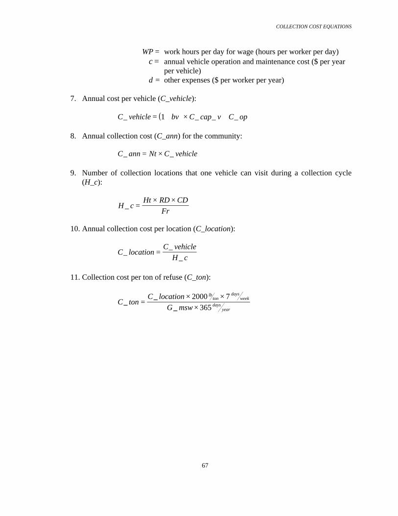
COLLECTION COST EQUATIONS
67
WP = work hours per day for wage (hours per worker per day) c = annual vehicle operation and maintenance cost ($ per year
per vehicle) d = other expenses ($ per worker per year)
7. Annual cost per vehicle (C_vehicle): ( )C vehicle bv C cap v C op_ _ _ _= + × +1 8. Annual collection cost (C_ann) for the community:
C ann Nt C vehicle_ _= ×
9. Number of collection locations that one vehicle can visit during a collection cycle(H_c):
H cHt RD CD
Fr_ =
× ×
10. Annual collection cost per location (C_location):
C locationC vehicle
H c_
_
_=
11. Collection cost per ton of refuse (C_ton):
C tonC location
G msw
lbton
daysweek
daysyear
__
_=
× ××
2000 7
365

COLLECTION COST EQUATIONS
68
3.4.2 Recyclables (C14 and C15)
Collection options C14 and C15 model collection of recyclables from multi-familydwellings that have been separated from the non-recyclable portion of multi-family refuse(“residuals”). Each collection location is supplied with one or more containers to holdrecyclable refuse. Option C14 covers pre-sorted recyclables deposited by residents intomultiple containers; option C15 is for commingled recyclables deposited in a singlecontainer. The annualized cost of the containers is treated as an additional capital cost.
The cost equations for options C14 and C15 are very similar in form to the cost equationsfor options C2, C3, and C4 for collection of residential recyclables. See Section 3.2.2.3for descriptions of the calculation methodology.
3.4.2.1 Generation Rate
The generation rate for recyclables (G_recyc) is found my multiplying the weeklycollection location waste generation rate (G_mf) by the fraction of recyclables removed or“captured” from the waste stream by residents (frac_cap_recyc). When the Collectionprocess model is used with the Optimization Model, the Optimization Model determineswhich components of the waste stream are collected by a particular collection option.When the Collection process model is used in stand-alone mode, the user specifies whichcomponents are collected. The method used to do this is described below.
The weekly recyclable generation rate for recyclables collection option j is calculated as:
G recyc G mf frac cap recycj j_ _ _ _= × ,
where: G recyc j_ = weekly recyclables generation rate for collection option j
where j is option C14 or C15 (pounds per week per location)
G mf_ = weekly multi-family MSW generation rate (pounds per location per week)
frac cap recyc j_ _ = captured recyclables fraction for collection option j
The captured recyclables fraction is found by summing the fraction of recyclable materialremoved by multi-family dwelling residents from each component of the multi-familyMSW stream. A table is provided in the Collection process model worksheet where theuser can enter values to indicate what fraction of each recyclable component is removedby participating residents from their mixed waste and deposited into recyclablescontainers. This fraction is referred to as the “capture rate” (cr). Entering a value of 0.75as the capture rate for aluminum cans, for instance, indicates that on average residents

COLLECTION COST EQUATIONS
69
successfully remove 75% of their aluminum cans from refuse and deposit them in arecyclables container. The other 25% is collected along with other non-capturedrecyclables and the residents’ non-recyclable refuse by another collection vehicle. Costsfor collection of this “residual” waste are accounted for in the Multi-Family ResidualWaste collection option (C16). Leaving a cell blank or entering a zero in the capture ratetable indicates that the component represented by that cell is not included in therecyclables collection program.
Default capture rates are assigned to the following multi-family waste streamcomponents:
• Old Newsprint• Old Corrugated Cardboard• Office Paper• Phone Books• Old Magazines• Third Class Mail• Paper - Other (5 classes)• Ferrous Cans• Ferrous Metal - Other• Aluminum Cans• Aluminum - Other (2 classes)• Clear Glass• Brown Glass• Green Glass• Translucent HDPE• Pigmented HDPE• PET• Plastic - Other (5 classes)
The Common process model contains listings of waste component weight fractions fortwo different multi-family waste compositions (MF_WT_FRAC_1 andMF_WT_FRAC_2). To determine the amount of recyclables removed from the wastestream (frac_cap_recyc), the Collection process model cell formulas multiply the user-specified/default capture rate for each waste component i (cri) by the correspondingweight fraction specified for that component in the MF_WT_FRAC_1 table.
frac recyc cr MF WT FRACj ii
_ _ _ _= ×∑ 1

COLLECTION COST EQUATIONS
70
where:
frac cap recyc j_ _ = captured recyclables fraction for collection option j
where j is C14 or C15 cri = capture rate for waste component i
MF WT FRAC_ _ _1 = weight fraction for waste component i of the Sector 1multi-family waste composition
3.4.2.2 Waste Density
Default values for the as-collected density of recyclable components of the multi-familywaste stream are listed in the Common process model (D_rcv). Default values for wastecomponent compaction factors (CF) are listed in the Input Parameters section of theCollection process model. Compaction factors represent the increased density of anywaste components that are compacted during collection. The default compaction factorvalues for all waste components are 1.0. The Collection process model uses these valuesand the default values of the individual component weight fractions for multi-familywaste Sector 1 listed in the Common process model (MF_WT_FRAC_1) to calculate anoverall density for multi-family recyclables in a recyclables collection vehicle:
D recycfrac cap recyc
cr MF WT FRAC
D rcv CF
j
j
ij i
i ii
__ _
_ _ _
_
= ×
×∑ 1
,
where:
D recyc j_ = overall density of recyclables for collection option j where j
is C4 or C15 (pounds per cubic yard) frac cap recyc j_ _ = captured recyclables fraction for collection option j
crij = capture rate for waste component i for collection option j
MF WT FRAC i_ _ _1 = weight fraction for waste component i of the Sector 1 multi-family waste composition
D rcvi_ = as-collected density of recyclables component i CFi = compaction factor for waste component i (pound per cubic
yard compacted density per pound per cubic yard as-collected density)
D_recyc can also be specified by the user. This is done by entering the desired value incell d_recyc in the Option C14 or C15 columns of the Input Parameters section of theCollection process model. Entering a value in one of these cells overrides the calculationprocedure described above, and the Collection process model uses the user-specifieddensity value in all subsequent calculations. If the d_recyc cell is empty, the Collectionprocess model calculates the overall density and uses the calculated value in subsequentcalculations.
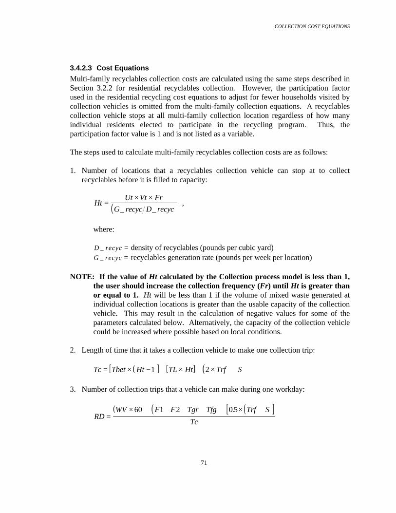
COLLECTION COST EQUATIONS
71
3.4.2.3 Cost Equations
Multi-family recyclables collection costs are calculated using the same steps described inSection 3.2.2 for residential recyclables collection. However, the participation factorused in the residential recycling cost equations to adjust for fewer households visited bycollection vehicles is omitted from the multi-family collection equations. A recyclablescollection vehicle stops at all multi-family collection location regardless of how manyindividual residents elected to participate in the recycling program. Thus, theparticipation factor value is 1 and is not listed as a variable.
The steps used to calculate multi-family recyclables collection costs are as follows:
1. Number of locations that a recyclables collection vehicle can stop at to collectrecyclables before it is filled to capacity:
( )HtUt Vt Fr
G recyc D recyc=
× ×_ _
,
where:
D recyc_ = density of recyclables (pounds per cubic yard) G recyc_ = recyclables generation rate (pounds per week per location)
NOTE: If the value of Ht calculated by the Collection process model is less than 1,the user should increase the collection frequency (Fr) until Ht is greater thanor equal to 1. Ht will be less than 1 if the volume of mixed waste generated atindividual collection locations is greater than the usable capacity of the collectionvehicle. This may result in the calculation of negative values for some of theparameters calculated below. Alternatively, the capacity of the collection vehiclecould be increased where possible based on local conditions.
2. Length of time that it takes a collection vehicle to make one collection trip:
( )[ ] [ ] ( )Tc Tbet Ht TL Ht Trf S= × − + × + × +1 2 3. Number of collection trips that a vehicle can make during one workday:
( ) ( ) ( )[ ]
RDWV F F Tgr Tfg Trf S
Tc=
× + + + + + × +60 1 2 0 5.
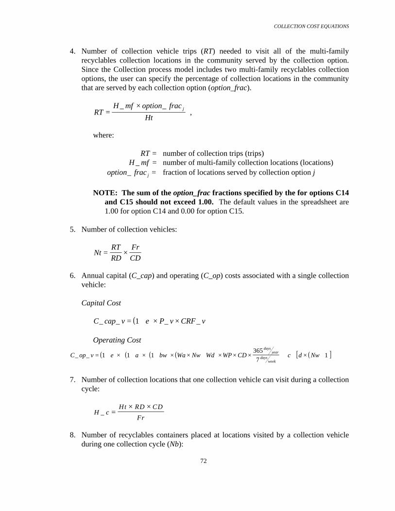
COLLECTION COST EQUATIONS
72
4. Number of collection vehicle trips (RT) needed to visit all of the multi-familyrecyclables collection locations in the community served by the collection option.Since the Collection process model includes two multi-family recyclables collectionoptions, the user can specify the percentage of collection locations in the communitythat are served by each collection option (option_frac).
RTH mf option frac
Htj=
×_ _ ,
where:
RT = number of collection trips (trips) H mf_ = number of multi-family collection locations (locations)
option frac j_ = fraction of locations served by collection option j
NOTE: The sum of the option_frac fractions specified by the for options C14and C15 should not exceed 1.00. The default values in the spreadsheet are1.00 for option C14 and 0.00 for option C15.
5. Number of collection vehicles:
NtRTRD
FrCD
= ×
6. Annual capital (C_cap) and operating (C_op) costs associated with a single collection
vehicle: Capital Cost
( )C cap v e P v CRF v_ _ _ _= + × ×1 Operating Cost
( ) ( ) ( ) ( ) ( )[ ]C op v e a bw Wa Nw Wd WP CD c d Nwdays
yeardays
week_ _ = + × + × + × × + × × ×
+ + × +
1 1 1
365
71
7. Number of collection locations that one collection vehicle can visit during a collection
cycle:
H cHt RD CD
Fr_ =
× ×
8. Number of recyclables containers placed at locations visited by a collection vehicle
during one collection cycle (Nb):
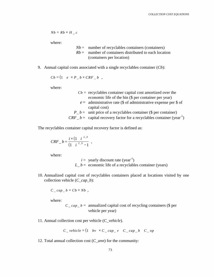
COLLECTION COST EQUATIONS
73
Nb Rb H c= × _
where:
Nb = number of recyclables containers (containers) Rb = number of containers distributed to each location
(containers per location) 9. Annual capital costs associated with a single recyclables container (Cb):
( )Cb e P b CRF b= + × ×1 _ _ , where:
Cb = recyclables container capital cost amortized over the economic life of the bin ($ per container per year)
e = administrative rate ($ of administrative expense per $ of capital cost)
P b_ = unit price of a recyclables container ($ per container) CRF b_ = capital recovery factor for a recyclables container (year-1)
The recyclables container capital recovery factor is defined as:
( )
( )CRF b
i i
i
L b
L b__
_=× ++ −
1
1 1 ,
where:
i = yearly discount rate (year-1) L b_ = economic life of a recyclables container (years)
10. Annualized capital cost of recyclables containers placed at locations visited by one
collection vehicle (C_cap_b):
C cap b Cb Nb_ _ = × , where: C cap b_ _ = annualized capital cost of recycling containers ($ per
vehicle per year) 11. Annual collection cost per vehicle (C_vehicle). ( )C vehicle bv C cap v C cap b C op_ _ _ _ _ _= + × + +1
12. Total annual collection cost (C_ann) for the community:

COLLECTION COST EQUATIONS
74
C ann Nt C vehicle_ _= ×
13. Annual collection cost per collection location (C_location):
C locationC vehicle
H c_
_
_=
14. Collection cost per ton of recyclables (C_ton):
C tonC location
G recyc
lbton
daysweek
daysyear
__
_=
× ××
2000 7
365

COLLECTION COST EQUATIONS
75
3.4.3 Residuals (C16)
Option C16 covers collection of the refuse discarded by residents of multi-familydwellings after the removal and separate collection of recyclables. The cost associatedwith recyclables collection is accounted for by options C14 and/or C15. There is noprovision in the Collection process model for separate collection of yard waste generatedby residents of multi-family dwellings.
3.4.3.1 Generation Rate
The waste generated for multi-family residual waste reflects the reduced weight of refuseset out for collection due to the removal of recyclables. G_residual is calculated asfollows:
G residual G mf
G recyc PF option frac
option frac
j j jj
jj
_ _
_ _
_= −
× ×∑∑ ,
where:
G residual_ = residual refuse generation rate (pounds per week per collection location)
G recyc j_ = recyclables generation rate for collection option j, where j is
options C14 and C15 (pounds per week per collection location)
PFj = participation factor for recyclables collection option j
option frac j_ = fraction of collection locations served by collection option j
3.4.3.2 Waste Density
The Collection process model calculates an overall density of residual refuse collected byoption C16 by averaging the density of the residuals at locations served by each of themulti-family recyclables collection options:
D residual
D residual option frac
option fracC
j jj
jj
_
_ _
_16 =×∑
∑ ,
where:
D residualC_ 16 = average density of residuals collected by option C16pounds per cubic yard)

COLLECTION COST EQUATIONS
76
D residual j_ = overall density of residuals set out by households served by
recyclables collection option j where j is C14 or C15 (pounds per cubic yard)
option frac j_ = fraction of households served by recyclables collection
option j
The overall density of residuals set out by households served by a particular recyclablescollection option is calculated as follows:
( )( )
( )D residual
PF cr MF WT FRAC
frac cap recyc D cv
PF MF WT FRAC
D cvj
j ij i
j i
j i
iii
__ _ _
_ _ _
_ _ _
_=
× − ×
− ×+
− ×
∑∑−
1 1
1
1 11
where:PFj = participation factor for recyclables collection option j where
j is C14 or C15 (participating households per total households)
crij = capture rate for recyclables component i for collection
option j MF WT FRAC i_ _ _1 = weight fraction for waste component i of the Sector 1
multi-family waste composition D cvi_ = compacted density of recyclables component
frac cap recyc j_ _ =captured recyclables fraction for collection option j
D_residualC16 can also be specified by the user. This is done by entering the desiredvalue in cell d_residual in the Option C16 column of the Input Parameters section of theCollection process model. Entering a value in this cell overrides the calculationprocedure described above, and the Collection process model uses the user-specifieddensity value in all subsequent calculations. If the d_residual cell is empty, theCollection process model calculates the average residual waste density as described aboveand uses the calculated value in subsequent calculations.
3.4.3.3 Cost Equations
The steps used to calculate residual collection costs are as follows:
1. Number of locations that a collection vehicle can stop at to collect residual wastebefore it is filled to capacity:
( )HtUt Vt Fr
G residual D residual=
× ×_ _
COLLECTION COST EQUATIONS
77
The remaining cost equations for Residuals collection are identical to the Mixed Waste(option C13) cost equations except that the mixed waste generation rate (G_msw) isreplaced by a residuals generation rate (G_residual). See Section 3.4.1.3 for a descriptionof the Mixed Waste cost equations.

COLLECTION COST EQUATIONS
78
3.4.4 Wet/Dry Collection
Collection options C17 and C18 model collection of multi-family dwelling waste whichhas been separated into wet, dry, and recyclable components by residents. Option C17models simultaneous collection of all three waste types by a three-compartment vehicle.Option C18 models collection of the wet and dry portions only using a two-compartmentvehicle; recyclables are collected by another vehicle. (The cost of recyclables collectionis accounted for using collection option C14 or C15.) The Collection process modelcalculates multi-family wet/dry collection costs using the methodology described inSection 3.2.6 for residential wet/dry collection. The reader should refer to that section fora more complete description of the calculation methodology.
3.4.4.1 Wet/Dry/Recyclables (C17)
The user may specify what fraction of each component of MSW will be collected as wetrefuse, dry refuse, and recyclables by making entries in the Wet/Dry/RecyclablesSeparation Factors table located in the Common process model. Component fractions arespecified by entering separation factor values (sf_WDR_weti, sf_WDR_dryi, orsf_WDR_recyci) between 0.00 and 1.00 in the appropriate cells to indicate the fraction ofeach component disposed of in a wet, dry, or recyclables container. Note: The wet, dry,and recyclables separation factors for each component of MSW must sum to 1.00.Thus, C17 cannot be used in conjunction with other multi-family collection options. Thecomponents listed below as “Wet” have default sf_WDR_weti values of 1.0; componentslisted as “Dry” have default sf_WDR_dryi values of 1.0. The components in the list ofrecyclables have a default sf_WDR_recyci value of 0.75 and a default sf_WDR_dryi valueof 0.25.

COLLECTION COST EQUATIONS
79
WET DRY RECYCLABLES
Leaves Non-recyclable paper Old NewsprintGrass clippings Non-recyclable ferrous metal Old CorrugatedBranches Non-recyclable aluminum CardboardFood waste Non-recyclable glass Office Paper
Non-recyclable plastic Paper - OtherMiscellaneous refuse Ferrous Cans
Ferrous Metal - OtherAluminum CansAluminum - OtherClear GlassBrown GlassGreen GlassTranslucent HDPEPigmented HDPEPETPlastic - Other
3.4.4.1.1 Dry Waste Generation Rate
The dry waste generation rate is the product of dry waste fraction (frac_dry) and theweekly multi-family waste generation rate:
G dry frac dry G mf_ _ _= × ,
where: G dry_ = weekly dry waste generation rate (pounds per week per
collection location)G mf_ = weekly multi-family waste generation rate (pounds per
week per collection location)
The dry refuse fraction (frac_dry) is the sum of the weight fractions specified for eachcomponent in the Sector 1 multi-family waste composition list in the Common processmodel multiplied by the corresponding dry refuse separation factor:
frac dry MF WT FRAC sf WDR dryi ii
_ _ _ _ _ _= ×∑ 1
where:
frac dry_ = dry refuse fractionMF WT FRAC i_ _ _1 = weight fraction for waste component i of the Sector 1
multi-family waste composition

COLLECTION COST EQUATIONS
80
sf WDR dryi_ _ = dry refuse separation factor for waste component i
3.4.4.1.2 Wet Waste Generation Rate
The wet waste generation rate is the product of the wet waste fraction (frac_wet) and thetotal weekly multi-family waste generation rate (G_mf):
G wet frac wet G mf_ _ _= × ,
where: G wet_ = weekly wet waste generation rate (pounds per week
per collection location)
The wet refuse fraction (frac_wet) is the sum of the weight fractions specified for eachcomponents in the Sector 1 multi-family waste composition list in the Common processmodel multiplied by the corresponding wet refuse separation factor:
frac wet MF WT FRAC sf WDR weti ii
_ _ _ _ _ _= ×∑ 1 ,
where:
frac wet_ = wet refuse fraction MF WT FRAC i_ _ _1 = weight fraction for waste component i of
the Sector 1 multi-family waste composition sf WDR weti_ _ = wet refuse separation factor for waste component i
3.4.4.1.3 Recyclables Generation Rate
The recyclables generation rate is the product of the captured recyclables fraction(frac_cap_recyc) and the total weekly multi-family waste generation rate (G_mf):
G recyc frac cap recyc G mf_ _ _ _= × ,
where: G recyc_ = weekly recyclables waste generation rate (pounds
per week per collection location)
The captured recyclables fraction (frac_cap_recyc) is the sum of the weight fractionsspecified for each component in the Sector 1 multi-family waste composition list in theCommon process model (MF_WT_FRAC_1) multiplied by the recyclables separationfactor specified for that component in the Common process model:

COLLECTION COST EQUATIONS
81
frac cap recyc MF WT FRAC sf WDR recyci ii
_ _ _ _ _ _ _= ×∑ 1 ,
where:
frac cap recyc_ _ = captured recyclables fraction MF WT FRAC i_ _ _1 = weight fraction for recyclable waste components
of the Sector 1 multi-family waste composition sf WDR recyci_ _ = recyclables separation factor for waste component i
3.4.4.1.4 Waste Densities
Unless the user enters override density values in the appropriate Input Parameter cells inthe C17 column, the Collection process model uses the default mixed waste collectionvehicle component densities (D_cv) listed in the Common process model to calculateoverall densities for dry and wet refuse. Default recyclables collection densities (D_rcv)and compaction factors (CF) are used to calculate an overall density for recyclables.Compaction factors represent the increased density of any recyclables components thatare compacted during collection. The default values for all waste components listed inthe Input Parameters section of the Collection process model are 1.0.
The dry refuse overall density is calculated as:
D dryfrac dry
sf WDR dry MF WT FRACD cv
i i
ii
__
_ _ _ _ _
_
= ×∑ 1 ,
where: D dry_ = overall density of dry refuse (pounds per cubic yard) frac dry_ = dry refuse fraction
sf WDR dryi_ _ = dry refuse separation factor for waste component i MF WT FRAC i_ _ _1 = weight fraction for waste component i of the Sector 1
multi-family waste composition D cvi_ = compacted density of component i (pounds per cubic yard)
The wet refuse overall density is calculated as:
D wetfrac wet
sf WDR wet MF WT FRACD cv
i i
ii
__
_ _ _ _ __
= ×∑ 1 ,
where: D wet_ = overall density of wet refuse (pounds per cubic yard)
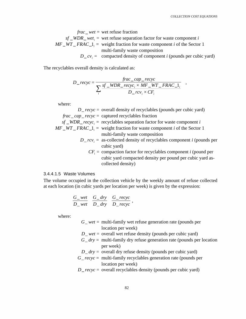
COLLECTION COST EQUATIONS
82
frac wet_ = wet refuse fraction sf WDR weti_ _ = wet refuse separation factor for waste component i
MF WT FRAC i_ _ _1 = weight fraction for waste component i of the Sector 1 multi-family waste composition
D cvi_ = compacted density of component i (pounds per cubic yard)
The recyclables overall density is calculated as:
D recycfrac cap recyc
sf WDR recyc MF WT FRACD rcv CF
i i
i ii
__ _
_ _ _ _ _
_
= ××
∑ 1 ,
where: D recyc_ = overall density of recyclables (pounds per cubic yard)
frac cap recyc_ _ = captured recyclables fraction sf WDR recyci_ _ = recyclables separation factor for waste component i
MF WT FRAC i_ _ _1 = weight fraction for waste component i of the Sector 1 multi-family waste composition
D rcvi_ = as-collected density of recyclables component i (pounds percubic yard)
CFi = compaction factor for recyclables component i (pound per cubic yard compacted density per pound per cubic yard as-collected density)
3.4.4.1.5 Waste Volumes
The volume occupied in the collection vehicle by the weekly amount of refuse collectedat each location (in cubic yards per location per week) is given by the expression:
G wetD wet
G dryD dry
G recycD recyc
_
_
_
_
_
_+ + ,
where: G wet_ = multi-family wet refuse generation rate (pounds per
location per week) D wet_ = overall wet refuse density (pounds per cubic yard) G dry_ = multi-family dry refuse generation rate (pounds per location
per week) D dry_ = overall dry refuse density (pounds per cubic yard) G recyc_ = multi-family recyclables generation rate (pounds per
location per week) D recyc_ = overall recyclables density (pounds per cubic yard)

COLLECTION COST EQUATIONS
83
3.4.4.1.6 Cost Equations
The steps used to calculate wet/dry/recyclables collection costs are as follows:
1. Number of collection locations that a wet/dry/recyclables collection vehicle can stopat before it is filled to capacity:
HtUt Vt Fr
G wetD wet
G dryD dry
G recycD recyc
=× ×
+ +
__
__
__
The remaining steps in the cost calculations for Option C17 are identical to those listed inSection 3.4.1.3 for Mixed Waste Collection (Option C13).
3.4.4.2 Wet/Dry (C18)
Collection Option C18 models wet/dry collection of waste from multi-family dwellingsthat are also served by a recyclables collection option. The waste collected by a C18wet/dry collection vehicle is the residual waste remaining after residents have removedsome portion of the recyclables for separate collection. The cost to collect this residualwaste must account for the recyclable material which residents did not separate from therest of their refuse, either because they chose not to participate in a recyclables collectionprogram or because they did not successfully remove 100% of each recyclable componentfrom the rest of their refuse. The collection cost must also account for how residentsdivide all of the residual waste between the wet and dry waste.
The user may specify what fraction of each component of MSW will be collected as wetrefuse and dry refuse by making entries in the Wet/Dry Separation Factors table located inthe Common process model. Component fractions are specified by entering separationfactor values (sf_WD_weti or sf_WD_dryi) between 0.00 and 1.00 in the appropriate cellsto indicate the fraction of each component disposed of in a wet, dry, or recyclablescontainer. Note: The wet and dry separation factors for each component of MSWmust sum to 1.00.
3.4.4.2.1 Dry Waste Generation Rate
The weekly dry refuse generation rate (G_dry) for Collection Option C18 is found bysumming the residual dry waste fractions calculated for each of the recyclables collectionoptions and multiplying the result by the weekly multi-family waste generation rate:
G dry G mf frac dry option fracj
j j_ _ _ _= × ×∑ ,
where:
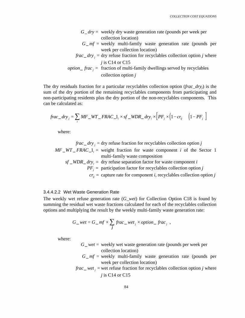
COLLECTION COST EQUATIONS
84
G dry_ = weekly dry waste generation rate (pounds per week percollection location)
G mf_ = weekly multi-family waste generation rate (pounds perweek per collection location)
frac dry j_ = dry refuse fraction for recyclables collection option j where
j is C14 or C15 option frac j_ = fraction of multi-family dwellings served by recyclables
collection option j
The dry residuals fraction for a particular recyclables collection option (frac_dryj) is thesum of the dry portion of the remaining recyclables components from participating andnon-participating residents plus the dry portion of the non-recyclables components. Thiscan be calculated as:
( ) ( )[ ]frac dry MF WT FRAC sf WDR dry PF cr PFj i i j ij ji
_ _ _ _ _ _= × × × − + −∑ 1 1 1
where:
frac dry j_ = dry refuse fraction for recyclables collection option j
MF WT FRAC i_ _ _1 = weight fraction for waste component i of the Sector 1multi-family waste composition
sf WDR dryi_ _ = dry refuse separation factor for waste component iPFj = participation factor for recyclables collection option j
crij = capture rate for component i, recyclables collection option j
3.4.4.2.2 Wet Waste Generation Rate
The weekly wet refuse generation rate (G_wet) for Collection Option C18 is found bysumming the residual wet waste fractions calculated for each of the recyclables collectionoptions and multiplying the result by the weekly multi-family waste generation rate:
G wet G mf frac wet option fracj
j j_ _ _ _= × ×∑ ,
where: G wet_ = weekly wet waste generation rate (pounds per week per
collection location)G mf_ = weekly multi-family waste generation rate (pounds per
week per collection location) frac wet j_ = wet refuse fraction for recyclables collection option j where
j is C14 or C15

COLLECTION COST EQUATIONS
85
option frac j_ = fraction of multi-family dwellings served by recyclables
collection option j
The wet residuals fraction for a particular recyclables collection option (frac_wetj) is thesum of the wet portion of the remaining recyclables components from participating andnon-participating residents plus the wet portion of the non-recyclables components. Thiscan be calculated as:
( ) ( )[ ]frac wet MF WT FRAC sf WDR wet PF cr PFj i i j ij ji
_ _ _ _ _ _= × × × − + −∑ 1 1 1 ,
where:
frac wet j_ = wet refuse fraction for recyclables collection option j
MF WT FRAC i_ _ _1 = weight fraction for waste component i of the Sector 1multi-family waste composition
sf WDR weti_ _ = wet refuse separation factor for waste component iPFj = participation factor for recyclables collection option j
crij = capture rate for component i, recyclables collection option j
3.4.4.2.3 Wet Waste Density
Unless the user enters override wet waste density in the d_wet Input Parameter cell in theC18 column, the Collection process model calculates the overall wet waste density byaveraging the overall wet densities of residual waste collected from multi-familydwellings served by different recyclables collection options:
D wet D wet option fracC j jj
_ _ _18 = ×∑where:
D wetC_ 18 = overall density of wet refuse collected by a C18 wet/dry collection vehicle (pounds per cubic yard)
D wet j_ = overall density of wet refuse from multi-family dwellings
served by recyclables collection option j, where j is C14 or C15
option frac j_ = fraction of multi-family dwellings served by recyclables
collection option j
The overall wet density of waste collected from locations that are served by a particularrecyclables collection option (D_wetj) must account for both the wet portions of the non-recyclable components of the waste stream and the wet portions of the recyclable
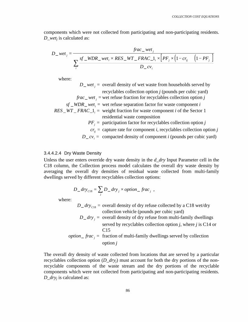
COLLECTION COST EQUATIONS
86
components which were not collected from participating and non-participating residents.D_wetj is calculated as:
( ) ( )[ ]D wet
frac wet
sf WDR wet RES WT FRAC PF cr PF
D cv
j
j
i i j ij j
ii
__
_ _ _ _ _
_
=× × × − + −
∑1 1 1
where: D wet j_ = overall density of wet waste from households served by
recyclables collection option j (pounds per cubic yard) frac wet j_ = wet refuse fraction for recyclables collection option j
sf WDR weti_ _ = wet refuse separation factor for waste component i RES WT FRAC i_ _ _1 = weight fraction for waste component i of the Sector 1
residential waste compositionPFj = participation factor for recyclables collection option j
crij = capture rate for component i, recyclables collection option j
D cvi_ = compacted density of component i (pounds per cubic yard)
3.4.4.2.4 Dry Waste Density
Unless the user enters override dry waste density in the d_dry Input Parameter cell in theC18 column, the Collection process model calculates the overall dry waste density byaveraging the overall dry densities of residual waste collected from multi-familydwellings served by different recyclables collection options:
D dry D dry option fracC j jj
_ _ _18 = ×∑ ,
where: D dryC_ 18 = overall density of dry refuse collected by a C18 wet/dry
collection vehicle (pounds per cubic yard) D dry j_ = overall density of dry refuse from multi-family dwellings
served by recyclables collection option j, where j is C14 or C15
option frac j_ = fraction of multi-family dwellings served by collection
option j
The overall dry density of waste collected from locations that are served by a particularrecyclables collection option (D_dryj) must account for both the dry portions of the non-recyclable components of the waste stream and the dry portions of the recyclablecomponents which were not collected from participating and non-participating residents.D_dryj is calculated as:
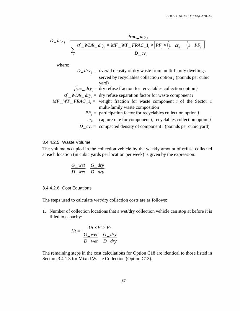
COLLECTION COST EQUATIONS
87
( ) ( )[ ]D dryfrac dry
sf WDR dry MF WT FRAC PF cr PF
D cv
j
j
i i j ij j
ii
__
_ _ _ _ _
_
=× × × − + −
∑1 1 1
where: D dry j_ = overall density of dry waste from multi-family dwellings
served by recyclables collection option j (pounds per cubic yard)
frac dry j_ = dry refuse fraction for recyclables collection option j
sf WDR dryi_ _ = dry refuse separation factor for waste component i MF WT FRAC i_ _ _1 = weight fraction for waste component i of the Sector 1
multi-family waste compositionPFj = participation factor for recyclables collection option j
crij = capture rate for component i, recyclables collection option j
D cvi_ = compacted density of component i (pounds per cubic yard)
3.4.4.2.5 Waste Volume
The volume occupied in the collection vehicle by the weekly amount of refuse collectedat each location (in cubic yards per location per week) is given by the expression:
G wetD wet
G dryD dry
_
_
_
_+
3.4.4.2.6 Cost Equations
The steps used to calculate wet/dry collection costs are as follows:
1. Number of collection locations that a wet/dry collection vehicle can stop at before it isfilled to capacity:
HtUt Vt Fr
G wetD wet
G dryD dry
=× ×
+
_
_
_
_
The remaining steps in the cost calculations for Option C18 are identical to those listed inSection 3.4.1.3 for Mixed Waste Collection (Option C13).

COLLECTION COST EQUATIONS
88
3.5 Commercial Waste Collection
Factories, stores, office buildings, etc. may use their own vehicles to transport wastegenerated on their sites to a disposal site. Or, they may contract with a privately ownedcollection service to provide vehicles for this purpose. However, the Collection processmodel calculates costs to collect commercial waste as though these costs are borne by thepublic sector, as they are assumed to be for residential and multi-family dwelling wastecollection.
The Collection process model models the collection of commercial waste the same waythat it models multi-family waste collection. Commercial businesses are assumed todispose of their waste in containers located at their places of business. Collectionvehicles are dispatched from a vehicle garage at the beginning of each workday to makethe rounds of these refuse container locations. Vehicles collect waste or recyclables untilthey reach capacity. Fully loaded vehicles drive to a treatment or disposal facility,unload, and begin another collection trip. At the end of the workday the vehicles returnto the vehicle garage.
The user can specify the total number of commercial waste collection locations (H_com)and the per capita generation rate for commercial waste (GR) in the appropriate data entrycells of the Common process model. Another cell in the Common process modelcalculates the average weekly waste generation rate per commercial waste collectionlocation (G_com):
( )G com
GR res pop mf pop
H com
daysweek
__ _
_=
× + × 7 ,
where: G com_ = weekly commercial waste generation rate (pounds per
location per week) GR = daily commercial waste generation rate (pounds per person
per day) res pop_ = number of people living in residential households (persons) mf pop_ = number of people living in multi-family dwellings
(persons) H com_ = number of commercial collection locations (locations)
There are two collection options provided in the Collection process model to describecommercial waste collection. Option C20 models collection of mixed refuse whileOption C19 models collection of commercial recyclables. If the user specifies that theparticipation factor for Option C19 is zero (i.e., no recycling), then Option C20 modelscollection of the entire waste stream. If the user specifies a non-zero recycling

COLLECTION COST EQUATIONS
89
participation factor for Option C19, then Option C20 models collection of the residualwaste.

COLLECTION COST EQUATIONS
90
3.5.1 Recyclables (C19)
Collection option C19 models collection of recyclables that have been separated from thenon-recyclable portion of commercial waste. The cost equations for options C19 are verysimilar in form to the cost equations for options C2, C3, and C4 for collection ofresidential recyclables. See Section 3.2.2.3 for a more detailed description of thecalculation methodology.
3.5.1.1 Generation Rate
The generation rate for recyclables (G_recyc) is found my multiplying the weeklycollection location waste generation rate (G_com) by the fraction of recyclables removedor “captured” from the waste stream by residents (frac_cap_recyc). When the Collectionprocess model is used with the Optimization Model, the Optimization Model determineswhich components of the waste stream are collected by a particular collection option.When the Collection process model is used in stand-alone mode, the user specifies whichcomponents are collected. The method used to do this is described below.
The weekly recyclable generation rate for recyclables collection option j is calculated as:
G recyc G com frac cap recyc_ _ _ _= × ,
where: G recyc_ = weekly commercial recyclables generation rate (pounds per
week per location) G com_ = weekly commercial MSW generation rate (pounds per
location per week) frac cap recyc_ _ = captured recyclables fraction
The captured recyclables fraction is found by summing the fraction of recyclable materialremoved by commercial businesses from each component of the commercial MSWstream. A table is provided in the Collection process model worksheet where the user canenter values to indicate what fraction of each recyclable component is removed byparticipating businesses from their mixed waste and deposited into recyclables containers.This fraction is referred to as the “capture rate” (cr). Entering a value of 0.75 as thecapture rate for aluminum cans, for instance, indicates that on average businessessuccessfully remove 75% of their aluminum cans from refuse and deposit them in arecyclables container. The other 25% is collected along with other non-capturedrecyclables and the business’ non-recyclable refuse by another collection vehicle. Costsfor collection of this “residual” waste are accounted for in the Commercial Mixed Wastecollection option (C20). Leaving a cell blank or entering a zero in the capture rate table

COLLECTION COST EQUATIONS
91
indicates that the component represented by that cell is not included in the recyclablescollection program.
Default capture rates are assigned to the following commercial waste stream components:
• Old Newsprint• Old Corrugated Cardboard• Office Paper• Phone Books• Third Class Mail• Paper - Other (3 classes)• Ferrous Cans• Ferrous Metal - Other• Aluminum Cans• Clear Glass• Brown Glass• Green Glass• PET• Other combustible/compostable/recyclable material• Other combustible/non-compostable/recyclable material
The Common process model contains listings of waste component weight fractions forten different commercial waste compositions. To determine the amount of recyclablesremoved from the waste stream (frac_cap_recyc), the Collection process model cellformulas multiply the user-specified/default capture rate for each waste component i (cri)by the corresponding weight fraction specified for that component in the Sector 1commercial waste composition table (COM_WT_FRAC_1).
frac recyc cr COM WT FRACii
_ _ _ _= ×∑ 1 ,
where:
frac cap recyc_ _ = captured recyclables fraction for collection option j where j is C14 or C15
cri = capture rate for waste component i COM WT FRAC_ _ _1 = weight fraction for waste component i of the Sector 1
commercial waste composition
3.5.1.2 Waste Density
Default values for the as-collected density of recyclable components of the commercialwaste stream are listed in the Common process model (D_rcv). Default values for wastecomponent compaction factors (CF) are listed in the Input Parameters section of the

COLLECTION COST EQUATIONS
92
Collection Processor. Compaction factors represent the increased density of wastecomponents that are compacted during collection. The default compaction factor valuefor all commercial waste components is 1.0. The Collection process model uses thesevalues and the default values of the individual component weight fractions forcommercial waste Sector 1 listed in the Common process model (COM_WT_FRAC_1) tocalculate an overall density for commercial recyclables in a recyclables collection vehicle:
D recycfrac cap recyc
cr COM WT FRACD rcv CF
i i
i ii
__ _
_ _ _
_
= ××
∑ 1 ,
where:
D recyc_ = overall density of (pounds per cubic yard) frac cap recyc_ _ = captured recyclables fraction
cri = capture rate for waste component i MF WT FRAC i_ _ _1 = weight fraction for waste component i of the Sector 1
commercial waste composition D rcvi_ = as-collected density of recyclables component i (pounds per
cubic yard) CFi = compaction factor for waste component i (pound per cubic
yard compacted density per pound per cubic yard as-collected density)
D_recyc can also be specified by the user. This is done by entering the desired value incell d_recyc in the Option C19 column of the Input Parameters section of the Collectionprocess model. Entering a value in this cell overrides the calculation procedure describedabove, and the Collection process model uses the user-specified density value in allsubsequent calculations. If the d_recyc cell is empty, the Collection process modelcalculates the overall density and uses the calculated value in subsequent calculations.
3.5.1.3 Cost Equations
Commercial recyclables collection costs are calculated using the same steps described inSection 3.2.2.3 for residential recyclables collection. However, the participation factorused in the residential recycling cost equations to adjust for fewer households visited bycollection vehicles is omitted from the commercial collection cost equations. Arecyclables collection vehicle stops at all commercial collection location regardless ofhow many individual businesses elected to participate in the recycling program. Thus,the participation factor value is 1 and is not listed as a variable.
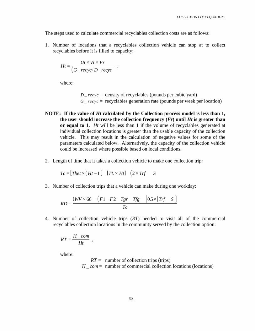
COLLECTION COST EQUATIONS
93
The steps used to calculate commercial recyclables collection costs are as follows:
1. Number of locations that a recyclables collection vehicle can stop at to collectrecyclables before it is filled to capacity:
( )HtUt Vt Fr
G recyc D recyc=
× ×_ _
,
where:
D recyc_ = density of recyclables (pounds per cubic yard) G recyc_ = recyclables generation rate (pounds per week per location)
NOTE: If the value of Ht calculated by the Collection process model is less than 1,the user should increase the collection frequency (Fr) until Ht is greater thanor equal to 1. Ht will be less than 1 if the volume of recyclables generated atindividual collection locations is greater than the usable capacity of the collectionvehicle. This may result in the calculation of negative values for some of theparameters calculated below. Alternatively, the capacity of the collection vehiclecould be increased where possible based on local conditions.
2. Length of time that it takes a collection vehicle to make one collection trip:
( )[ ] [ ] ( )Tc Tbet Ht TL Ht Trf S= × − + × + × +1 2 3. Number of collection trips that a vehicle can make during one workday:
( ) ( ) ( )[ ]
RDWV F F Tgr Tfg Trf S
Tc=
× + + + + + × +60 1 2 0 5.
4. Number of collection vehicle trips (RT) needed to visit all of the commercial
recyclables collection locations in the community served by the collection option:
RTH com
Ht=
_ ,
where:
RT = number of collection trips (trips) H com_ = number of commercial collection locations (locations)

COLLECTION COST EQUATIONS
94
5. Number of collection vehicles:
NtRTRD
FrCD
= ×
6. Annual capital (C_cap) and operating (C_op) costs associated with a single collection
vehicle: Capital Cost
( )C cap v e P v CRF v_ _ _ _= + × ×1 Operating Cost
( ) ( ) ( ) ( ) ( )[ ]C op v e a bw Wa Nw Wd WP CD c d Nwdays
yeardays
week_ _ = + × + × + × × + × × ×
+ + × +
1 1 1
365
71
7. Number of collection locations that one collection vehicle can visit during a collection
cycle:
H cHt RD CD
Fr_ =
× ×
8. Number of recyclables containers placed at locations visited by a collection vehicle
during one collection cycle (Nb):
Nb Rb H c= × _ , where:
Nb = number of recyclables containers (containers) Rb = number of containers distributed to each location
(containers per location) 9. Annual capital costs associated with a single recyclables container (Cb):
( )Cb e P b CRF b= + × ×1 _ _
where:
Cb = recyclables container capital cost amortized over the economic life of the bin ($ per container per year)
e = administrative rate ($ of administrative expense per $ of capital cost)
P b_ = unit price of a recyclables container ($ per container) CRF b_ = capital recovery factor for a recyclables container (year-1)
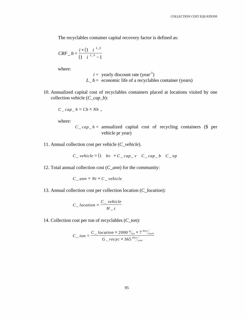
COLLECTION COST EQUATIONS
95
The recyclables container capital recovery factor is defined as:
( )
( )CRF b
i i
i
L b
L b__
_=× ++ −
1
1 1 where:
i = yearly discount rate (year-1) L b_ = economic life of a recyclables container (years)
10. Annualized capital cost of recyclables containers placed at locations visited by one
collection vehicle (C_cap_b):
C cap b Cb Nb_ _ = × , where:
C cap b_ _ = annualized capital cost of recycling containers ($ pervehicle pr year)
11. Annual collection cost per vehicle (C_vehicle). ( )C vehicle bv C cap v C cap b C op_ _ _ _ _ _= + × + +1
12. Total annual collection cost (C_ann) for the community:
C ann Nt C vehicle_ _= × 13. Annual collection cost per collection location (C_location):
C locationC vehicle
H c_
_
_=
14. Collection cost per ton of recyclables (C_ton):
C tonC location
G recyc
lbton
daysweek
daysyear
__
_=
× ××
2000 7
365
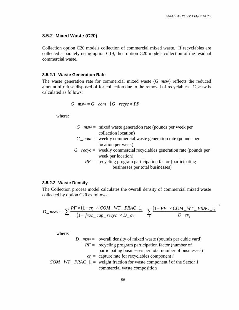
COLLECTION COST EQUATIONS
96
3.5.2 Mixed Waste (C20)
Collection option C20 models collection of commercial mixed waste. If recyclables arecollected separately using option C19, then option C20 models collection of the residualcommercial waste.
3.5.2.1 Waste Generation Rate
The waste generation rate for commercial mixed waste (G_msw) reflects the reducedamount of refuse disposed of for collection due to the removal of recyclables. G_msw iscalculated as follows:
( )G msw G com G recyc PF_ _ _= − ×
where:
G msw_ = mixed waste generation rate (pounds per week per collection location)
G com_ = weekly commercial waste generation rate (pounds per location per week)
G recyc_ = weekly commercial recyclables generation rate (pounds per week per location)
PF = recycling program participation factor (participating businesses per total businesses)
3.5.2.2 Waste Density
The Collection process model calculates the overall density of commercial mixed wastecollected by option C20 as follows:
( )( )
( )D msw
PF cr COM WT FRAC
frac cap recyc D cv
PF COM WT FRACD cv
i i
i
i
iii
__ _ _
_ _ _
_ _ _
_=
× − ×
− ×+
− ×
∑∑
−1 1
1
1 11
where: D msw_ = overall density of mixed waste (pounds per cubic yard)
PF = recycling program participation factor (number of participating businesses per total number of businesses)
cri = capture rate for recyclables component i COM WT FRAC i_ _ _1 = weight fraction for waste component i of the Sector 1
commercial waste composition

COLLECTION COST EQUATIONS
97
D cvi_ = compacted density of waste component i (pounds per cubic yard)
frac cap recyc_ _ = captured recyclables fraction for collection option C19
D_msw can also be specified by the user. This is done by entering the desired value incell d_msw in the Option C20 column of the Input Parameters section of the Collectionprocess model. Entering a value in this cell overrides the calculation procedure describedabove, and the Collection process model uses the user-specified density value in allsubsequent calculations. If the d_msw cell is empty, the Collection process modelcalculates the overall density and uses the calculated value in subsequent calculations.
3.5.2.3 Cost Equations
The steps used to calculate commercial mixed waste collection costs are as follows:
1. Number of locations that a collection vehicle can stop at to collect residual wastebefore it is filled to capacity:
( )HtUt Vt Fr
G msw D msw=
× ×_ _
NOTE: If the value of Ht calculated by the Collection process model is less than 1,the user should increase the collection frequency (Fr) until Ht is greater thanor equal to 1. Ht will be less than 1 if the volume of mixed waste generated atindividual collection locations is greater than the usable capacity of the collectionvehicle. This may result in the calculation of negative values for some of theparameters calculated below. Alternatively, the capacity of the collection vehiclecould be increased where possible based on local conditions.
The remaining cost equations for commercial mixed waste collection are identical to theMixed Waste (option C13) cost equations. See Section 3.4.1.3 for a description of theMixed Waste cost equations.
COLLECTION VEHICLE CALCULATION PARAMETERS
98
4. COLLECTION VEHICLE CALCULATION PARAMETERS
The calculations performed in the Collection process model to determine LCI parameterconsumption and release rates are based in part on a common set of collection vehicleparameters. Once calculated from user input or default values, they are used repeatedly insubsequent calculations. To avoid repetition in this document, the equations used tocalculate these parameters are described in Chapter 4. References to the appropriatesection of this chapter are provided when these parameters are used in the calculationsdescribed in later chapters.

COLLECTION VEHICLE CALCULATION PARAMETERS
99
4.1 Daily Activity Durations
The following equations are used to calculate the length of time that an individualcollection vehicle spends performing various activities during one workday. Some ofthese times are specified directly by the user or are provided as default values. The othersare derived from values of collection cost parameters previously described in Chapter 3.These times are used to calculate fuel consumption associated with stop and go driving onthe collection route and fuel consumption associated with other driving activities.
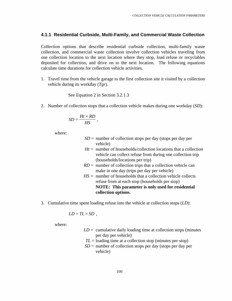
COLLECTION VEHICLE CALCULATION PARAMETERS
100
4.1.1 Residential Curbside, Multi-Family, and Commercial Waste Collection
Collection options that describe residential curbside collection, multi-family wastecollection, and commercial waste collection involve collection vehicles traveling fromone collection location to the next location where they stop, load refuse or recyclablesdeposited for collection, and drive on to the next location. The following equationscalculate time durations for collection vehicle activities.
1. Travel time from the vehicle garage to the first collection site it visited by a collectionvehicle during its workday (Tgr).
See Equation 2 in Section 3.2.1.3
2. Number of collection stops that a collection vehicle makes during one workday (SD):
SDHt RD
HS=
× ,
where: SD = number of collection stops per day (stops per day per
vehicle) Ht = number of households/collection locations that a collection
vehicle can collect refuse from during one collection trip (households/locations per trip)
RD = number of collection trips that a collection vehicle can make in one day (trips per day per vehicle)
HS = number of households that a collection vehicle collects refuse from at each stop (households per stop)
NOTE: This parameter is only used for residential collection options.
3. Cumulative time spent loading refuse into the vehicle at collection stops (LD):
LD TL SD= × ,
where: LD = cumulative daily loading time at collection stops (minutes
per day per vehicle) TL = loading time at a collection stop (minutes per stop)
SD = number of collection stops per day (stops per day per vehicle)

COLLECTION VEHICLE CALCULATION PARAMETERS
101
4. Travel time between collection stops (Tbtw):
See Equation 3 in Section 3.2.1.3
5. Cumulative daily travel time between collection stops (Tb):
( )[ ]Tb SD RD Tbtwstopday= − × ×1 ,
where: Tb = cumulative daily travel time between collection stops
(minutes per day per vehicle) SD = number of collection stops per day (stops per day per
vehicle) RD = number of collection trips that a collection vehicle can
make in one day (trips per day per vehicle) Tbtw = average travel time between adjacent collection stops (minutes)
6. Travel time between start/end of a collection route and the disposal facility (Trf):
See Equation 4 in Section 3.2.1.3
7. Cumulative daily time spent traveling between starting or ending points of collectionroutes and the disposal facility (F_R):
( )[ ]F R RD Trf_ .= × + ×2 0 5 ,
where: F R_ = cumulative daily travel time between collection route and
disposal facility (minutes per day per vehicle) RD = number of collection trips that a collection vehicle can
make in one day (trips per day per vehicle)Trf = travel time between start/end of collection route and the
disposal facility (minutes per trip)
8. Cumulative daily time spent unloading refuse at the disposal facility (UD):
( )UD RD S= + ×0 5. ,
where:UD = cumulative daily unloading time at disposal site (minutes
per day per vehicle)

COLLECTION VEHICLE CALCULATION PARAMETERS
102
RD = number of collection trips that a collection vehicle can make in one day (trips per day per vehicle)
S = unloading time at disposal site (minutes per trip)
9. Travel time from the disposal facility to the vehicle garage at the end of the workday(Tfg):
See Equation 5 in Section 3.2.1.3

COLLECTION VEHICLE CALCULATION PARAMETERS
103
4.1.2 Recyclables Drop-Off
Residential waste collection option C8 covers collection of recyclable material thatresidents have deposited in roll-on/roll-off containers at a centrally located drop-off site.Collection vehicles are dispatched from a garage to collect the accumulated material andtransport it to a treatment or disposal facility. Instead of making a sequence of stops tocollect refuse, the collection vehicles make round trips between the waste sites and therecyclables treatment or disposal facility. The following equations calculate collectionvehicle travel times between the vehicle garage, the collection site, and thetreatment/disposal facility, and the time spent loading and unloading recyclables.
1. Travel time from the vehicle garage to the collection site (Tgr):
See Equation 2 in Section 3.2.1.3.
2. Cumulative daily time spent loading recyclables into the vehicle at the collection site(LD):
LD TL RD= ×
where: LD = cumulative daily loading time at the collection site (minutes
per day per vehicle) TL = loading time at the collection site (minutes per stop) RD = collection trips per day (trips per day per vehicle)
3. Travel time between collection site and the treatment/disposal facility (Trf):
See Equation 3 in Section 3.2.1.3.
4. Cumulative daily time spent traveling between the collection site and the treatment ordisposal facility (F_S):
( )[ ]F S RD Trf_ = × − ×2 1
5. Cumulative daily time spent unloading recyclables at the treatment/disposal facility(UD):
UD RD S= ×
6. Travel time from the treatment/disposal facility to the vehicle garage at the end of theworkday (Tfg). See Equation 5 in Section 3.2.1.3

COLLECTION VEHICLE CALCULATION PARAMETERS
104
4.2 Daily Service Hours
Service hours are the length of time that a vehicle is used for collection activities,excluding lunch and other breaks. The parameter “service hours per day” is used tocalculate the frequency of maintenance activities that result in LCI parameterconsumption and/or release rates such as vehicle washdowns and motor fluidreplacement.
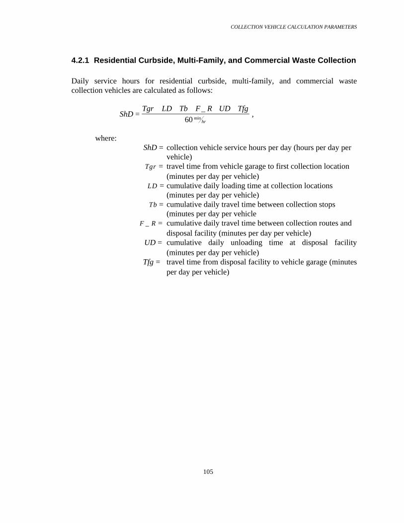
COLLECTION VEHICLE CALCULATION PARAMETERS
105
4.2.1 Residential Curbside, Multi-Family, and Commercial Waste Collection
Daily service hours for residential curbside, multi-family, and commercial wastecollection vehicles are calculated as follows:
ShDTgr LD Tb F R UD Tfg
minhr
=+ + + + +_
60 ,
where:ShD = collection vehicle service hours per day (hours per day per
vehicle) Tgr = travel time from vehicle garage to first collection location
(minutes per day per vehicle) LD = cumulative daily loading time at collection locations
(minutes per day per vehicle) Tb = cumulative daily travel time between collection stops
(minutes per day per vehicle F R_ = cumulative daily travel time between collection routes and
disposal facility (minutes per day per vehicle)UD = cumulative daily unloading time at disposal facility
(minutes per day per vehicle)Tfg = travel time from disposal facility to vehicle garage (minutes
per day per vehicle)

COLLECTION VEHICLE CALCULATION PARAMETERS
106
4.2.2 Recyclables Drop-Off
Daily service hours for a collection vehicle that services a recyclables drop-off collectionsite are calculated as follows:
ShDTgr LD F R UD Tfg
minhr
=+ + + +_
60 ,
where:
ShD = collection vehicle service hours per day (hours per day per vehicle)
Tgr = travel time from vehicle garage to the collection site (minutes per day per vehicle)
LD = cumulative daily loading time at the collection site (minutes per day per vehicle)
F R_ = cumulative daily travel time between the collection site andte treatment/disposal facility (minutes per day per vehicle)
UD = cumulative daily unloading time at the treatment/disposal facility (minutes per day per vehicle)
Tfg = travel time from treatment/disposal facility to vehiclegarage (minutes per day per vehicle)

COLLECTION VEHICLE CALCULATION PARAMETERS
107
4.3 Daily Miles Traveled
The number of miles traveled per day by a collection vehicle is used to calculate mileage-based LCI parameters including air emissions and consumption of vehicle maintenanceitems such as engine oil.

COLLECTION VEHICLE CALCULATION PARAMETERS
108
4.3.1 Residential Curbside, Multi-Family, and Commercial Waste Collection
The following equations are used to calculate the total distance that a residential curbside,multi-family, or commercial waste collection vehicle travels during one workday.
1. Distance vehicle travels from vehicle garage to the starting point of the first collectionroute (Dgr):
DgrVgr Tgr
minhr
=×
60 ,
where: Dgr = distance from garage to start of first collection
route (miles per day per vehicle) Vgr = average travel speed between garage and start of first
collection route (miles per hour) Tgr = travel time from garage to start of first collection route
(minutes per day per vehicle) 2. Cumulative daily distance traveled between collection stops (Db):
DbVbet Tb
minhr
=×
60 ,
where: Db = cumulative daily distance traveled between collection stops
(miles per day per vehicle) Vbet = average travel speed between collection stops (miles per hour) Tb = cumulative daily travel time between collection stops
(minutes per day) 3. Cumulative daily distance traveled between start/end points of collection routes and
the treatment or disposal facility (DF_R):
DF RVfr F R
hr_
_min
=×
60 ,
where: DF R_ = cumulative daily distance between start/end of collection
routes and the treatment/disposal facility (miles per day per vehicle)
Vrf = average travel speed between start/end of collection route and the disposal facility (miles per hour)

COLLECTION VEHICLE CALCULATION PARAMETERS
109
F R_ = cumulative travel time between start/end of collection routes and the disposal facility (minutes per day per vehicle)
4. Distance from the treatment or disposal facility to the vehicle garage (Dfg):
DfgVfg Tfg
hr=
×60 min
,
where:Dfg = distance from treatment/disposal facility to the garage
(miles per day per vehicle)Vfg = average travel speed between disposal facility and garage
(miles per hour)Tfg = travel time from disposal facility to garage at the end of the
workday (minutes per day per vehicle)
5. Total distance traveled by a collection vehicle during one workday (MiD):
MiD Dgr Db DF R Dfg= + + +_ ,
where:MiD = total miles traveled per day (miles per day per vehicle)

COLLECTION VEHICLE CALCULATION PARAMETERS
110
4.3.2 Recyclables Drop-Off
The following equations are used to calculate the distance that a recyclables drop-offcollection vehicle travels during one workday.
1. Distance vehicle travels from vehicle garage to the collection site at the beginning ofits workday (Dgr):
DgrVgr Tgr
minhr
=×
60 2. Cumulative daily distance traveled between the collection site and the recyclables
treatment/disposal facility (DF_S):
DF SVrf F S
minhr
__
=×
60,
where: DF S_ = cumulative daily distance traveled between the collection
site and the treatment/disposal facility (miles per day per vehicle)
Vrf = average travel speed between the collection site and the treatment/disposal facility (miles per hour)
F S_ = cumulative travel time between the collection site and the treatment/disposal facility (minutes per day per vehicle)
3. Distance from the treatment/disposal facility to the vehicle garage (Dfg):
DfgVfg Tfg
hr=
×60 min
4. Total distance traveled by a collection vehicle during one workday (MiD):
MiD Dgr DF R Dfg= + +_
COLLECTION VEHICLE CALCULATION PARAMETERS
111
4.4 Daily Fuel Usage
The parameter “gallons of fuel per day per vehicle” (Fuel_D) is used to calculate energyconsumption rates, airborne pollutant release rates, and waterborne pollutant release rates.

COLLECTION VEHICLE CALCULATION PARAMETERS
112
4.4.1 Residential Curbside, Multi-Family, and Commercial Waste Collection
The following equations are used to calculate the amount of fuel used by a residentialcurbside, multi-family, or commercial waste collection vehicle during one day’sactivities. Total daily fuel usage is the sum of the fuel burned while the vehicle istraveling (garage to first collection route; between collection stops; between collectionroute and disposal facility; disposal facility to garage) and the fuel burned while thevehicle is stopped with its engine idling (loading at collection stops; unloading at disposalsite).
1. Daily fuel usage while traveling (fuel_trav):
( ) ( ) ( ) ( )
fuel travTgr Vgr F R Vrf Tfg Vfg
MPG trav cvTb Vbet
MPG btwn cvminhr
minhr
__
_ _ _ _=
× + × + ××
+×
×60 60 ,
where: fuel trav_ = daily collection vehicle fuel usage while traveling (gallons
per day per vehicle) MPG trav cv_ _ = collection vehicle fuel consumption rate while traveling
(miles per gallon) MPG btwn cv_ _ = collection vehicle fuel consumption rate while traveling
between collection stops (miles per gallon) 2. Daily fuel usage while idling (fuel_idle):
( )
fuel idleLD UD GPH idle cv
minhr
__ _
=+ ×
60,
where: fuel idle_ = daily collection vehicle fuel usage while traveling (gallons
per day per vehicle) GPH idle cv_ _ = collection rate fuel consumption rate while idling (gallons
per hour) 3. Total daily fuel usage (FuelD):
FuelD fuel trav fuel idle= +_ _ ,

COLLECTION VEHICLE CALCULATION PARAMETERS
113
where:
FuelD = daily collection vehicle fuel usage (gallons per day per vehicle)

COLLECTION VEHICLE CALCULATION PARAMETERS
114
4.4.2 Recyclables Drop-Off
The following equations are used to calculate the amount of fuel used by a recyclablesdrop-off collection vehicle during one day’s activities. Total daily fuel usage is the sumof the fuel burned while the vehicle is traveling (garage to collection site; betweencollection site and treatment/disposal facility; treatment/disposal facility to garage) andthe fuel burned while the vehicle is stopped with its engine idling (loading at collectionsite; unloading at treatment/disposal facility).
1. Daily fuel usage while traveling (fuel_trav).
( ) ( ) ( )
fuel travTgr Vgr F S Vrf Tfg Vfg
MPG trav cv minhr
__
_ _=
× + × + ×× 60
2. Daily fuel usage while idling (fuel_idle).
( )
fuel idleLD UD GPH idle cv
minhr
__ _
=+ ×
60 3. Total daily fuel usage (FuelD).
FuelD fuel trav fuel idle= +_ _
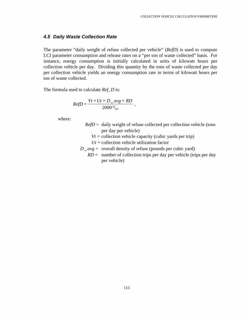
COLLECTION VEHICLE CALCULATION PARAMETERS
115
4.5 Daily Waste Collection Rate
The parameter “daily weight of refuse collected per vehicle” (RefD) is used to computeLCI parameter consumption and release rates on a “per ton of waste collected” basis. Forinstance, energy consumption is initially calculated in units of kilowatt hours percollection vehicle per day. Dividing this quantity by the tons of waste collected per dayper collection vehicle yields an energy consumption rate in terms of kilowatt hours perton of waste collected.
The formula used to calculate Ref_D is:
RefD =× × ×Vt Ut D avg RD
lbton
_
2000 ,
where: RefD = daily weight of refuse collected per collection vehicle (tons
per day per vehicle) Vt = collection vehicle capacity (cubic yards per trip) Ut = collection vehicle utilization factor
D avg_ = overall density of refuse (pounds per cubic yard)RD = number of collection trips per day per vehicle (trips per day
per vehicle)

ENERGY CONSUMPTION EQUATIONS
116
5. ENERGY CONSUMPTION EQUATIONS
The Collection process model uses default or user-supplied data on fuel consumed bycollection vehicles, drop-off vehicles (options C8 and C10 only), and electricityconsumed at the vehicle garage to calculate the total amount of energy consumed per tonof material collected. Energy consumption is expressed in terms of British Thermal Unitsper ton of waste collected (Btu per ton).
The Collection process model accounts for two types of energy associated with both fueland electricity. The fuel energy calculations include (1) the energy released when fuel iscombusted in a collection vehicle or a resident’s drop-off vehicle and (2) the energyexpended to manufacture the fuel from petroleum feed stock. This second form of energyis called “pre-combustion energy”. Likewise for electricity usage, the calculationsinclude (1) the Btu value of the electricity consumed at the vehicle garage and (2) thepre-combustion energy associated with the production of the fuels used to generate theelectricity consumed at the vehicle garage. Default data relating fuel combustion andpre-combustion energy to air, water, and solid waste emissions are found in the Commonprocess model. Default data on the Btu value of electricity, including its pre-combustionenergy, are located in the Electrical Energy process model.
For all collection options except C8 and C10, the total energy consumption rate per ton ofrefuse collected is expressed by:
E ton E cv ton E gar ton_ _ _ _ _= + ,
where: E ton_ = total energy consumption rate (Btu per ton) E cv ton_ _ = collection vehicle energy consumption rate (Btu per ton)E gar ton_ _ = garage energy consumption rate (Btu per ton)
For collection option C8 (recyclables drop-off by residents using their own vehicles;transfer of recyclables from the drop-off site to a treatment/disposal site using collectionvehicles), the total energy consumption rate is given by:
E ton E cv ton E gar ton E dov ton_ _ _ _ _ _ _= + + ,
where: E dov ton_ _ = drop-off vehicle energy consumption rate (Btu per ton)

ENERGY CONSUMPTION EQUATIONS
117
For collection option C10 (yard waste drop-off at a treatment/disposal site by residentsusing their own vehicles), the total energy consumption rate is given by:
tondovEtonE ___ =

ENERGY CONSUMPTION EQUATIONS
118
5.1 Collection Vehicles
Energy consumption by collection vehicles is the sum of the energy consumed by thecombustion of diesel fuel plus the pre-combustion energy associated with production ofdiesel fuel from petroleum feedstock.
1. Fuel usage per ton of refuse (FuelTon).
FuelTonFuelDRefD
= ,
where: FuelTon = fuel usage per ton of refuse (gallons per ton)
FuelD = daily collection vehicle fuel usage (gallons per day per vehicle)
RefD = daily weight of refuse collected per vehicle (tons per dayper vhicle)
2. Fuel combustion energy per ton of refuse (E_fuel_ton). E fuel ton FuelTon dsl enrg_ _ _= × , where: E fuel ton_ _ = fuel combustion energy consumption rate (Btu per ton) dsl enrg_ = energy content of diesel fuel (Btu per gallon) 3. Pre-combustion energy per ton of refuse (E_pc_ton). E pc ton FuelTon dsl pc enrg_ _ _ _= × , where: E pc ton_ _ = fuel pre-combustion energy consumption rate (Btu per ton) dsl pc enrg_ _ = pre-combustion energy content of diesel fuel (Btu per
gallon) 4. Total collection vehicle energy consumption per ton of refuse (E_cv_ton).
E cv ton E fuel ton E pc ton_ _ _ _ _ _= +

ENERGY CONSUMPTION EQUATIONS
119
5.2 Drop-Off Vehicles
The fuel energy consumed by drop-off vehicles is a function of the round trip distancethey travel between a residence and the drop-off site, their fuel consumption rate whiletraveling (expressed in miles per gallon), the fraction of trips they make that are dedicatedsolely to recyclables or yard waste drop-off (versus trips made for other purposes thatinclude refuse drop-off as a secondary objective), the weight of refuse carried per trip,and the Btu value of the fuel they consume (including both combustion and pre-combustion energy).
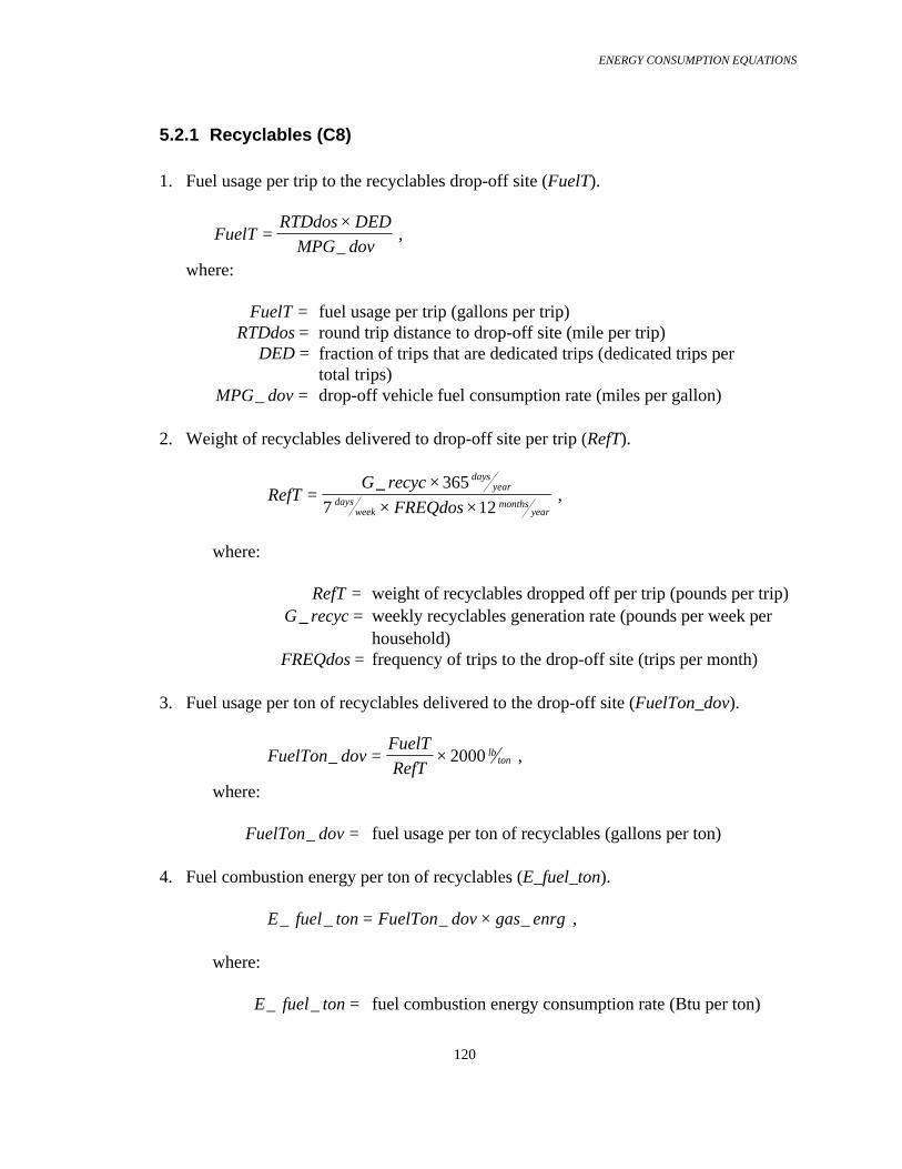
ENERGY CONSUMPTION EQUATIONS
120
5.2.1 Recyclables (C8)
1. Fuel usage per trip to the recyclables drop-off site (FuelT).
FuelTRTDdos DED
MPG dov=
×_
,
where: FuelT = fuel usage per trip (gallons per trip) RTDdos = round trip distance to drop-off site (mile per trip) DED = fraction of trips that are dedicated trips (dedicated trips per
total trips) MPG dov_ = drop-off vehicle fuel consumption rate (miles per gallon) 2. Weight of recyclables delivered to drop-off site per trip (RefT).
RefTG recyc
FREQdos
daysyear
daysweek
monthsyear
=×
× ×_ 365
7 12 ,
where: RefT = weight of recyclables dropped off per trip (pounds per trip) G recyc_ = weekly recyclables generation rate (pounds per week per
household) FREQdos = frequency of trips to the drop-off site (trips per month) 3. Fuel usage per ton of recyclables delivered to the drop-off site (FuelTon_dov).
FuelTon dovFuelTRefT
lbton_ = × 2000 ,
where: FuelTon dov_ = fuel usage per ton of recyclables (gallons per ton) 4. Fuel combustion energy per ton of recyclables (E_fuel_ton). E fuel ton FuelTon dov gas enrg_ _ _ _= × , where: E fuel ton_ _ = fuel combustion energy consumption rate (Btu per ton)

ENERGY CONSUMPTION EQUATIONS
121
gas enrg_ = energy content of gasoline (Btu per gallon) 5. Pre-combustion energy per ton of recyclables (E_pc_ton). E pc ton FuelTon dov gas pc enrg_ _ _ _ _= × , where: E pc ton_ _ = fuel pre-combustion energy consumption rate (Btu per ton) gas pc enrg_ _ = pre-combustion energy content of gasoline (Btu per
gallon) 6. Total drop-off vehicle energy consumption per ton of recyclables (E_dov_ton).
E dov ton E fuel ton E pc ton_ _ _ _ _ _= + ,
where:
E dov ton_ _ = drop-off vehicle energy consumption rate (Btu per ton)
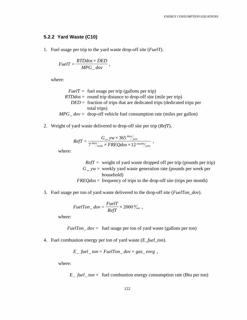
ENERGY CONSUMPTION EQUATIONS
122
5.2.2 Yard Waste (C10)
1. Fuel usage per trip to the yard waste drop-off site (FuelT).
FuelTRTDdos DED
MPG dov=
×_
,
where: FuelT = fuel usage per trip (gallons per trip) RTDdos = round trip distance to drop-off site (mile per trip) DED = fraction of trips that are dedicated trips (dedicated trips per
total trips) MPG dov_ = drop-off vehicle fuel consumption rate (miles per gallon) 2. Weight of yard waste delivered to drop-off site per trip (RefT).
RefTG yw
FREQdos
daysyear
daysweek
monthsyear
=×
× ×_ 365
7 12 ,
where: RefT = weight of yard waste dropped off per trip (pounds per trip) G yw_ = weekly yard waste generation rate (pounds per week per
household) FREQdos = frequency of trips to the drop-off site (trips per month) 3. Fuel usage per ton of yard waste delivered to the drop-off site (FuelTon_dov).
FuelTon dovFuelTRefT
lbton_ = × 2000 ,
where: FuelTon dov_ = fuel usage per ton of yard waste (gallons per ton) 4. Fuel combustion energy per ton of yard waste (E_fuel_ton). E fuel ton FuelTon dov gas enrg_ _ _ _= × , where: E fuel ton_ _ = fuel combustion energy consumption rate (Btu per ton)
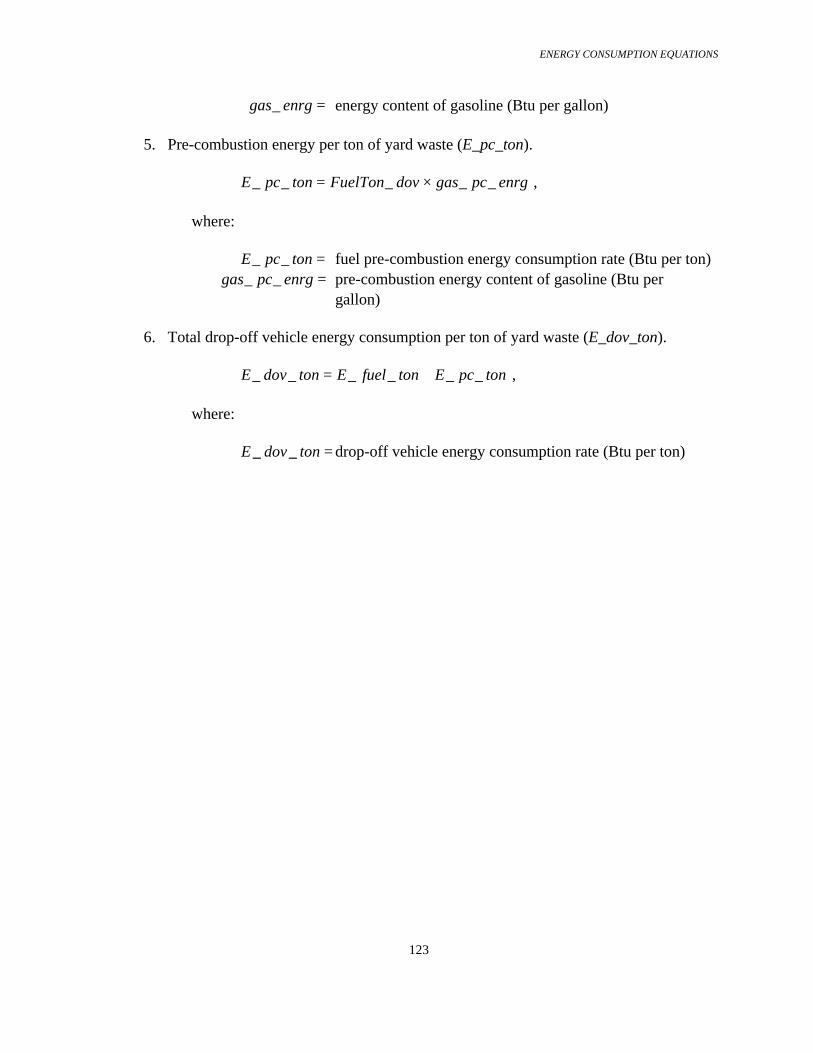
ENERGY CONSUMPTION EQUATIONS
123
gas enrg_ = energy content of gasoline (Btu per gallon) 5. Pre-combustion energy per ton of yard waste (E_pc_ton). E pc ton FuelTon dov gas pc enrg_ _ _ _ _= × , where: E pc ton_ _ = fuel pre-combustion energy consumption rate (Btu per ton) gas pc enrg_ _ = pre-combustion energy content of gasoline (Btu per
gallon) 6. Total drop-off vehicle energy consumption per ton of yard waste (E_dov_ton).
E dov ton E fuel ton E pc ton_ _ _ _ _ _= + ,
where:
E dov ton_ _ = drop-off vehicle energy consumption rate (Btu per ton)

ENERGY CONSUMPTION EQUATIONS
124
5.3 Garage
The collection vehicle garage includes both a covered maintenance area and an office.The energy consumed at the collection vehicle garage per ton of refuse is a function of thegarage area per collection vehicle, the electricity consumed per unit of garage area, theweight of refuse collected per vehicle, and the Btu value of the electricity (including thepre-combustion energy associated with generation of the electricity). The Btu value ofelectricity used in the Collection process model is the regional Btu value per aggregatekilowatt hour of electricity. This value is obtained from the Electric Energy processmodel.
1. Electricity consumed per collection vehicle (ElecD).
( ) ( )ElecD maint area maint elec off area off elec= × + ×_ _ _ _ , where: ElecD = electricity consumed per collection vehicle (kWh per
vehicle) maint area_ = garage maintenance area per collection vehicle (ft2 per
vehicle) maint elec_ = garage maintenance area electricity consumption rate (kWh
per ft2) off area_ = garage office area per collection vehicle (ft2 per vehicle) off elec_ = garage office area electricity consumption rate (kWh per
ft2) 2. Electricity consumed per ton of refuse (ElecTon).
ElecTonElecDRefD
= ,
where: ElecTon = electricity consumed per ton of refuse (kWh per ton) 3. Energy consumed at garage per ton of refuse (E_gar_ton).
E gar ton ElecTon region btu per elec kwh_ _ _ _ _ _= × ,

ENERGY CONSUMPTION EQUATIONS
125
where:
region btu per elec kwh_ _ _ _ = regional Btu value per aggregate kilowatt hour of electricity (Btu per kWh)
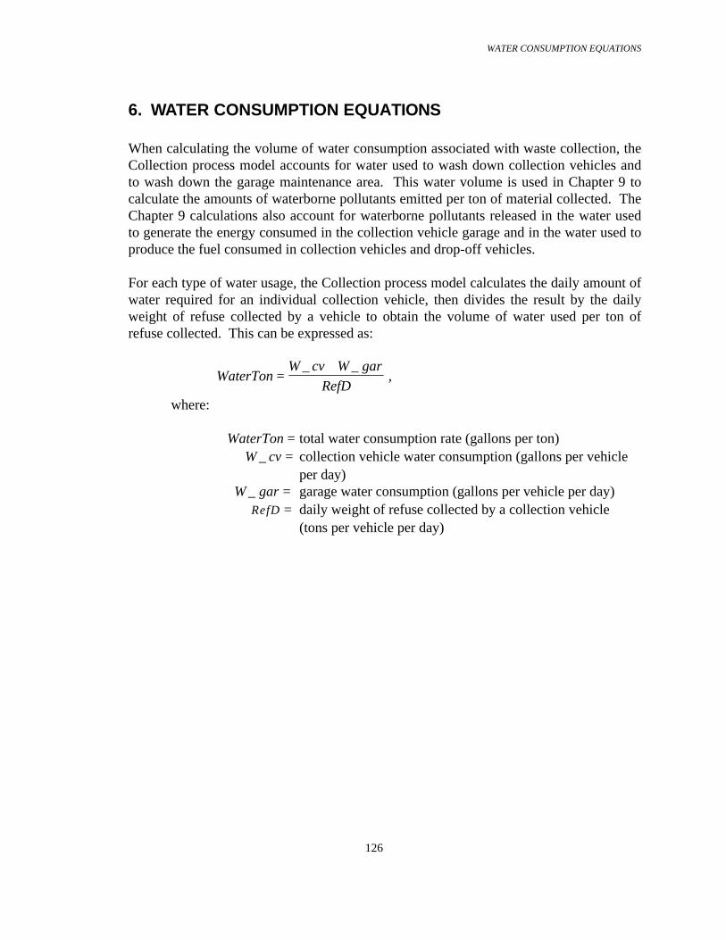
WATER CONSUMPTION EQUATIONS
126
6. WATER CONSUMPTION EQUATIONS
When calculating the volume of water consumption associated with waste collection, theCollection process model accounts for water used to wash down collection vehicles andto wash down the garage maintenance area. This water volume is used in Chapter 9 tocalculate the amounts of waterborne pollutants emitted per ton of material collected. TheChapter 9 calculations also account for waterborne pollutants released in the water usedto generate the energy consumed in the collection vehicle garage and in the water used toproduce the fuel consumed in collection vehicles and drop-off vehicles.
For each type of water usage, the Collection process model calculates the daily amount ofwater required for an individual collection vehicle, then divides the result by the dailyweight of refuse collected by a vehicle to obtain the volume of water used per ton ofrefuse collected. This can be expressed as:
WaterTonW cv W gar
RefD=
+_ _ ,
where:
WaterTon = total water consumption rate (gallons per ton) W cv_ = collection vehicle water consumption (gallons per vehicle
per day) W gar_ = garage water consumption (gallons per vehicle per day)
RefD = daily weight of refuse collected by a collection vehicle (tons per vehicle per day)
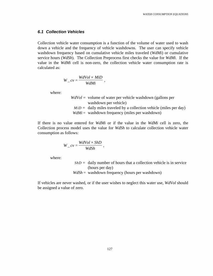
WATER CONSUMPTION EQUATIONS
127
6.1 Collection Vehicles
Collection vehicle water consumption is a function of the volume of water used to washdown a vehicle and the frequency of vehicle washdowns. The user can specify vehiclewashdown frequency based on cumulative vehicle miles traveled (WdMi) or cumulativeservice hours (WdSh). The Collection Preprocess first checks the value for WdMi. If thevalue in the WdMi cell is non-zero, the collection vehicle water consumption rate iscalculated as:
W cvWdVol MiD
WdMi_ =
× ,
where: WdVol = volume of water per vehicle washdown (gallons per
washdown per vehicle) MiD = daily miles traveled by a collection vehicle (miles per day) WdMi = washdown frequency (miles per washdown)
If there is no value entered for WdMi or if the value in the WdMi cell is zero, theCollection process model uses the value for WdSh to calculate collection vehicle waterconsumption as follows:
W cvWdVol ShD
WdSh_ =
× ,
where: ShD = daily number of hours that a collection vehicle is in service
(hours per day) WdSh = washdown frequency (hours per washdown)
If vehicles are never washed, or if the user wishes to neglect this water use, WdVol shouldbe assigned a value of zero.

WATER CONSUMPTION EQUATIONS
128
6.2 Garage
Daily water consumption associated with the garage is found by calculating the volume ofwater used to wash down the maintenance area of the garage. It is calculated on a pervehicle basis to keep its units consistent with those for vehicle washdowns.
W gar maint wd vol maint area WdD_ _ _ _= × × ,
where:
maint wd vol_ _ = volume of washdown water per unit area (gallons per ft2 perwashdown)
maint area_ = garage maintenance area per collection vehicle (ft2 per vehicle)
WdD = garage washdown frequency (washdowns per day)

AIRBORNE RELEASE EQUATIONS
129
7. AIRBORNE RELEASE EQUATIONS
The Collection process model calculates the amounts (by weight) of airborne pollutantsemitted per ton of material collected using the miles traveled and fuel consumed bycollection vehicles and electricity consumed at the vehicle garage. These calculations aremade for all collection options except for option C10 (yard waste drop-off) which doesnot use collection vehicles. The equations for options C8 (recyclables drop-off) and C10include the emissions associated with fuel consumed in the vehicles residents use to dropoff their refuse at collection sites. Airborne release rates are expressed in terms of poundsof pollutant per ton of waste collected.
Release rates are calculated for the following airborne pollutants:
• Carbon monoxide• Nitrogen oxides• Total Particulates (particulate matter greater than 10 microns)• PM10 (particulate matter smaller than 10 microns)• Carbon dioxide emissions from fossil fuel sources• Carbon dioxide emissions from biomass fuel sources• Sulfur oxides• Hydrocarbons, excluding methane• Methane• Lead• Ammonia• Hydrochloric acid
The Collection process model also calculates values for the Greenhouse Gas Equivalenceof the emissions associated with each collection option. This calculation is described inSection 7.4.
The Collection process model accounts for two forms of airborne pollutant emissionsassociated with the fuel combusted in vehicles. The fuel emission calculations include(1) the pollutants released when fuel is combusted in a collection vehicle or a resident’sdrop-off vehicle and (2) the pollutants emitted when the fuel was refined from petroleumfeed stock. This second form of release is called “pre-combustion emissions”. Similarly,the emissions calculations for electricity consumed at the vehicle garage include (1) thepollutants released when the electricity was generated and (2) the pre-combustionemissions associated with the production of the fuels used to generate the electricity.Default values for fuel combustion emission factors (EFp, where p is a particularpollutant) are listed in the Input Parameter section of the Collection process model.Default values for pre-combustion emission factors for diesel fuel (d_emp) and gasoline(g_emp) are found in the Common process model. Default values for electricity

AIRBORNE RELEASE EQUATIONS
130
generation emission factors (r_totp) are located in the Electrical Energy process model.These factors include pre-combustion emissions.
For all collection options except C8 and C10, the total airborne release rate per ton ofrefuse collected for pollutant p is expressed by:
A ton A cv ton A gar tonp p p_ _ _ _ _= + ,
where: A tonp_ = total airborne release rate of pollutant p (pounds per ton)
A cv tonp_ _ = collection vehicle emission rate of pollutant p (pounds per
ton) A gar tonp_ _ = garage emission rate of pollutant p (pounds per ton)
For collection option C8 (recyclables drop-off with collection vehicles used to transferrecyclables from the drop-off site to a disposal site), the total airborne release rate is givenby:
A ton A cv ton A gar ton A dov tonp p p p_ _ _ _ _ _ _= + + ,
where:
A dov tonp_ _ = drop-off vehicle emission rate of pollutant p (pounds per
ton)
For collection option C10 (yard waste drop-off at a disposal site), the total airbornerelease rate is given by:
A ton A dov tonp p_ _ _=
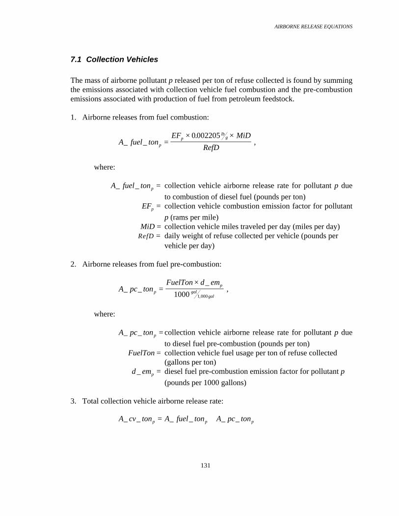
AIRBORNE RELEASE EQUATIONS
131
7.1 Collection Vehicles
The mass of airborne pollutant p released per ton of refuse collected is found by summingthe emissions associated with collection vehicle fuel combustion and the pre-combustionemissions associated with production of fuel from petroleum feedstock.
1. Airborne releases from fuel combustion:
A fuel tonEF MiD
RefDp
plb
g_ _
.=
× ×0 002205 ,
where:
A fuel tonp_ _ = collection vehicle airborne release rate for pollutant p due
to combustion of diesel fuel (pounds per ton)EFp = collection vehicle combustion emission factor for pollutant
p (rams per mile) MiD = collection vehicle miles traveled per day (miles per day) RefD = daily weight of refuse collected per vehicle (pounds per
vehicle per day)
2. Airborne releases from fuel pre-combustion:
A pc tonFuelTon d em
p
p
galgal
_ __
,
=×
1000 1 000
,
where:
A pc tonp_ _ = collection vehicle airborne release rate for pollutant p due
to diesel fuel pre-combustion (pounds per ton) FuelTon = collection vehicle fuel usage per ton of refuse collected
(gallons per ton) d emp_ = diesel fuel pre-combustion emission factor for pollutant p
(pounds per 1000 gallons) 3. Total collection vehicle airborne release rate:
A cv ton A fuel ton A pc tonp p p_ _ _ _ _ _= +

AIRBORNE RELEASE EQUATIONS
132
7.2 Drop-Off Vehicles
The mass of airborne pollutant p released per ton of recyclables or yard waste dropped offat a collection or disposal site is found by summing the emissions associated with drop-off vehicle fuel combustion and the pre-combustion emissions associated with productionof fuel from petroleum feedstock.
1. The fuel combustion air pollutant emission rate for drop-off vehicles is a function ofthe round trip distance they travel between a residence and the drop-off site, thefraction of trips they make that are dedicated solely to recyclables or yard waste drop-off (versus trips made for other purposes that include refuse drop-off as a secondaryobjective), the weight of material carried per trip, and the emission factor for aparticular pollutant:
A fuel tonRTDdos DED EF
RefTp
plb
glb
ton_ _
.=
× × × ×0 002205 2000 ,
where:
RTDdos = round trip distance to drop-off site (mile per trip) DED = fraction of trips that are dedicated trips (dedicated trips per
total trips) RefT = weight of material dropped off per trip (pounds per trip)
2. The pre-combustion air pollutant emission rate for drop-off vehicles is a function of
the volume of fuel (assumed to be gasoline) consumed per ton of refuse and the pre-combustion emission factor for a particular pollutant:
A pc tonFuelTon dov g em
p
p
galgal
_ __ _
,
=×
1000 1 000
,
where: A pc tonp_ _ = drop-off vehicle airborne release rate for pollutant p due to
gasoline pre-combustion (pounds per ton) FuelTon dov_ = drop-off vehicle fuel usage per ton of recyclables (gallons
per ton) g emp_ = gasoline pre-combustion emission factor for pollutant p
(pounds per 1000 gallons)

AIRBORNE RELEASE EQUATIONS
133
3. Total drop-off vehicle airborne release rate:
A cv ton A fuel ton A pc tonp p p_ _ _ _ _ _= +

AIRBORNE RELEASE EQUATIONS
134
7.3 Garage
The airborne emission rates associated with the electricity consumed at the collectionvehicle garage are a function of the garage area per collection vehicle, the electricityconsumed per unit of garage area, the weight of refuse collected per vehicle, and thepollutant emission rate per kilowatt hour of electricity (including the pre-combustionenergy associated with generation of the electricity). The pollutant emission rates used inthe Collection process model are the regional total emissions per aggregate kilowatt hourof electricity. These values are obtained from the Electric Energy process model in unitsof pounds per kilowatt hour.
1. Electricity consumed per collection vehicle (ElecD):
( ) ( )ElecD maint area maint elec off area off elec= × + ×_ _ _ _ 2. Electricity consumed per ton of refuse (ElecTon):
ElecTonElecDRefD
=
3. Airborne emission rate of pollutant p per ton of refuse (A_gar_tonp):
A gar ton ElecTon r totp p_ _ _= ×
where:
r tot p_ = regional total emission rate of pollutant p per aggregate
kilowatt hour of electricity (pound per kWh)

AIRBORNE RELEASE EQUATIONS
135
7.4 Greenhouse Gas Equivalence
The Collection process model calculates Greenhouse Gas Equivalence per ton of refuse(GGE) collected for four atmospheric releases: carbon dioxide (CO2), methane (CH4),nitrogen oxides (NOx), and other hydrocarbons (HC). It is calculated as:
GGE A ton GWPp p p= ×_ ,
where: GGE p = Greenhouse Gas Equivalence per ton for pollutant p
where p is CO2, CH4, NOx, or HC (equivalents per ton) A ton p_ = total airborne release rate of pollutant p (pounds per ton)
GWPp = Relative 20-year Global Warming Potential for pollutant p
(equivalents per pound)
The Greenhouse Gas Equivalence per ton of refuse from all four components is summedand reported as Total Greenhouse Gas Equivalence per ton of refuse:
GGE GGEtotal pp
= ∑

WATERBORNE RELEASE EQUATIONS
136
8. WATERBORNE RELEASE EQUATIONS
The Collection process model uses the previously described consumption parametersWaterTon (gallons of water consumed per ton of refuse collected), FuelTon (gallons offuel consumed per ton of refuse), and ElecTon (kilowatts of electricity consumed per tonof refuse) to calculate the amounts of waterborne pollutants emitted per ton of materialcollected. Waterborne release rates are expressed in terms of pounds of pollutant per tonof material collected.
Release rates are calculated for the following waterborne pollutants:
• Dissolved Solids• Suspended Solids• Biochemical Oxygen Demand• Chemical Oxygen Demand• Oil• Sulfuric Acid• Iron• Ammonia• Copper• Cadmium• Arsenic• Mercury• Phosphate• Selenium• Chromium• Lead• Zinc
The Collection process model accounts for two types of waterborne pollutant emissionsassociated with generation of the electricity consumed at the vehicle garage. Thewaterborne release calculations include (1) the pollutants released when the electricityconsumed at the garage was generated and (2) the pre-combustion emissions associatedwith the production of the fuels used to generate electricity. Waterborne releasesassociated with fuel combustion are assumed to be nil, so the fuel emission calculationsonly include pre-combustion waterborne pollutants. Default values for electricitygeneration waterborne pollutant emission factors (r_totp , where p is particular pollutant)are located in the Electrical Energy process model. Default values for pre-combustionwaterborne pollutant emission factors for diesel fuel (d_emp) and gasoline (g_emp) arefound in the Common process model.

WATERBORNE RELEASE EQUATIONS
137
For all collection options except C8 and C10, the total waterborne release rate per ton ofrefuse collected for pollutant p is expressed by:
W ton W cv ton W gar tonp p p_ _ _ _ _= + ,
where: W tonp_ = total waterborne emission rate of pollutant p (pounds per
ton) W cv tonp_ _ = collection vehicle emission rate of pollutant p (pounds per
ton) W gar tonp_ _ = garage emission rate of pollutant p (pounds per ton)
For collection option C8 (recyclables drop-off with collection vehicles used to transferrecyclables from the drop-off site to a disposal site), the total waterborne release rate isgiven by:
W ton W cv ton W gar ton W dov tonp p p p_ _ _ _ _ _ _= + + ,
where:
W dov tonp_ _ = drop-off vehicle emission rate of pollutant p (pounds per
ton)
For collection option C10 (yard waste drop-off at a disposal site), the total waterbornerelease rate is given by:
W ton W dov tonp p_ _ _=

WATERBORNE RELEASE EQUATIONS
138
8.1 Collection Vehicles
The mass of waterborne pollutant p released per ton of refuse collected is found bysumming the emissions associated with water usage and the pre-combustion emissionsassociated with production of fuel from petroleum feedstock.
1. Waterborne releases from water usage (vehicle and garage washdown water):
W water ton WaterTon EFp p_ _ = × ,
where:
W water tonp_ _ = collection vehicle waterborne release rate for pollutant p
due to water consumption (pounds per ton) WaterTon = collection vehicle water consumption rate (gallons per ton)
EFp = washdown water emission factor for pollutant p
(pounds per gallon)
2. Waterborne releases from fuel pre-combustion:
W pc tonFuelTon d em
p
p
galgal
_ __
,
=×
1000 1 000
,
where: W pc tonp_ _ = collection vehicle waterborne release rate for
pollutant p due to diesel fuel pre-combustion (pounds per ton)
FuelTon = collection vehicle fuel usage per ton of refuse collected (gallons per ton)
d emp_ = diesel fuel pre-combustion emission factor for pollutant p
(pounds per 1000 gallons) 3. Total collection vehicle waterborne release rate:
W cv ton W water ton W pc tonp p p_ _ _ _ _ _= +
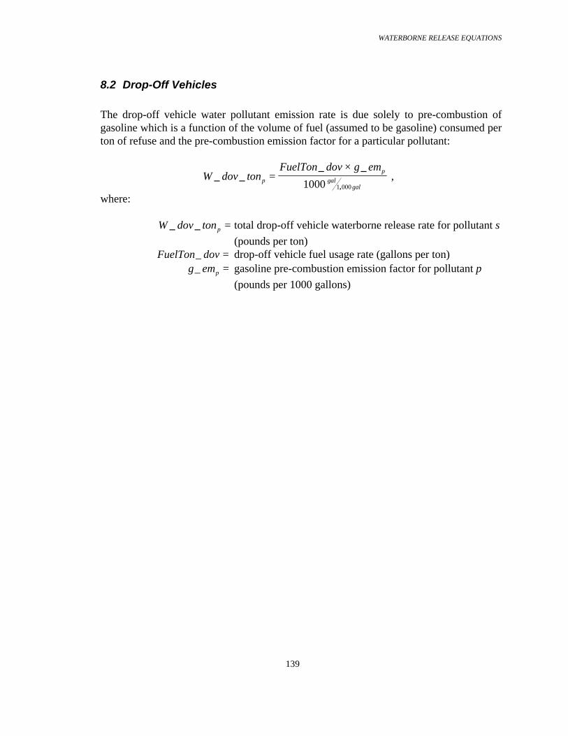
WATERBORNE RELEASE EQUATIONS
139
8.2 Drop-Off Vehicles
The drop-off vehicle water pollutant emission rate is due solely to pre-combustion ofgasoline which is a function of the volume of fuel (assumed to be gasoline) consumed perton of refuse and the pre-combustion emission factor for a particular pollutant:
W dov tonFuelTon dov g em
p
p
galgal
_ __ _
,
=×
1000 1 000
,
where: W dov tonp_ _ = total drop-off vehicle waterborne release rate for pollutant s
(pounds per ton) FuelTon dov_ = drop-off vehicle fuel usage rate (gallons per ton) g emp_ = gasoline pre-combustion emission factor for pollutant p
(pounds per 1000 gallons)

WATERBORNE RELEASE EQUATIONS
140
8.3 Garage
The waterborne emission rates associated with the electricity consumed at the collectionvehicle garage are a function of the electricity consumed per ton of refuse collected andthe pollutant emission rate per kilowatt hour of electricity (including the pre-combustionemissions associated with production of the fuel used to generate the electricity). Thepollutant emission rates used in the Collection process model are the regional totalemissions per aggregate kilowatt hour of electricity. These values are obtained from theElectric Energy process model in units of pounds of pollutant per kilowatt hour.
W gar ton ElecTon r totp p_ _ _= ×
where:
ElecTon = electricity consumed per ton of refuse (kWh per ton) r tot p_ = regional total emission rate of pollutant p per aggregate
kilowatt hour of electricity (pounds per kWh)

SOLID WASTE GENERATION EQUATIONS
141
9. SOLID WASTE GENERATION EQUATIONS
The Collection process model uses previously described consumption parameters tocalculate the amount of solid waste generated by collection vehicles, drop-off vehicles,and the collection vehicle garage. The generation rates of the solid waste by-products offuel and energy consumption are expressed in terms of pounds of solid waste per ton ofrefuse collected. Generation rates for miscellaneous waste items such as tires and enginefluids are expressed in terms appropriate for the particular item.
Solid wastes associated with fuel combustion are negligible, so the fuel emissioncalculations only include pre-combustion solid wastes (i.e., wastes created when the fuelwas refined from petroleum feedstock). The Collection process model accounts for twotypes of solid waste associated with generation of the electricity consumed at the vehiclegarage: (1) the solid waste produced by the combustion of fuel to generate electricity and(2) the pre-combustion solid waste associated with the production of the fuels used togenerate electricity. Default values for five categories of electricity solid wastegeneration factors are located in the Electrical Energy process model (r_tots, where s is asolid waste category). Default values for fuel pre-combustion solid waste generationfactors for diesel fuel (d_ems) and gasoline (g_ems) are found in the Common processmodel.
For all collection options except C8 and C10, the total generation rate per ton of refusecollected for solid waste s is expressed by:
SW ton SW cv ton SW gar tons s s_ _ _ _ _= + ,
where:
SW tons_ = total generation rate for solid waste s (pounds per ton)
SW cv tons_ _ = collection vehicle generation rate for solid waste s (pounds per ton)
SW gar tons_ _ = garage generation rate for solid waste s (pounds per ton)
For collection option C8 (recyclables drop-off with collection vehicles used to transferrecyclables from the drop-off site to a disposal site), the total solid waste generation rateis given by:
SW ton SW cv ton SW gar ton SW dov tons s s s_ _ _ _ _ _ _= + + ,

SOLID WASTE GENERATION EQUATIONS
142
where:
SW dov tons_ _ = drop-off vehicle generation rate for solid waste s (poundper ton)
For collection option C10 (yard waste drop-off at a disposal site), the total solid wastegeneration rate is given by:
SW ton SW dov tons s_ _ _=

SOLID WASTE GENERATION EQUATIONS
143
9.1 Collection Vehicles
The mass of solid waste s released per ton of refuse collected is found by calculating thepre-combustion emissions associated with production of fuel from petroleum feedstock.
SW pc tonFuelTon d em
ps
galgal
_ __
,
=×
1000 1 000
,
where: SW pc tons_ _ = collection vehicle generation rate for solid waste s due to
diesel fuel pre-combustion (pounds per ton) FuelTon = collection vehicle fuel usage per ton of refuse collected
(gallons per ton) d ems_ = diesel fuel pre-combustion emission factor for solid waste s
(pounds per 1000 gallons)

SOLID WASTE GENERATION EQUATIONS
144
9.2 Drop-Off Vehicles
The drop-off solid waste rate is a function of the volume of fuel (assumed to be gasoline)consumed per ton of recyclables or yard waste dropped off at a collection site and the pre-combustion emission factor for a particular category of solid waste:
SW dov tonFuelTon dov g em
ss
galgal
_ __ _
,
=×
1000 1 000
,
where: SW dov tons_ _ = total drop-off vehicle generation rate for solid waste s
(pounds per ton) FuelTon dov_ = drop-off vehicle fuel usage rate (gallon per ton) g ems_ = gasoline pre-combustion emission factor for solid waste s
(pounds per 1000 gallons)

SOLID WASTE GENERATION EQUATIONS
145
9.3 Garage
The solid waste generation rates associated with the electricity consumed at the collectionvehicle garage are a function of the electricity consumed per ton of refuse collected andthe waste generation rates per kilowatt hour of electricity (including the pre-combustionwaste associated with production of fuel used to generate the electricity). The solid wastegeneration rates used in the Collection process model are the regional total emissions peraggregate kilowatt hour of electricity. These values are obtained from the Electric Energyprocess model in units of pounds per kilowatt hour.
SW gar ton ElecTon r tots s_ _ _= ×
where:
SW gar tons_ _ = garage generation rate for solid waste s (pounds per ton) ElecTon = electricity consumed per ton of refuse (kWh per ton)
r tots_ = regional total emission rate of solid waste s per aggregate kilowatt hour of electricity (pounds per kWh)
REFERENCES
146
10. REFERENCES
Barlaz, M. A. and R. Ranjithan (1995). “System Description for a Life-Cycle Inventoryof Municipal Solid Waste Management Alternatives.” North Carolina State University,Department of Civil Engineering.
Kaneko, A. (1995). “Solid Waste Systems Analysis and Landfill Utilization Policy.”North Carolina State University, Department of Civil Engineering: Ph.D. Dissertation.
Tchobanoglous, G., H. Theisen, and S. Vigil (1993). Integrated Solid WasteManagement. McGraw-Hill, Inc., New York.
USEPA, 1993. “Life Cycle Design Guidance Manual - Environmental Requirements andThe Product System.” EPA/600/R-92/226.
U.S. Bureau of Labor Statistics (USBLS, 1996), Producer Price Indexes, monthly andannual.

147
Appendices
Appendix A
148
APPENDIX A
DEFAULT INPUT VALUES(FOR VARIABLES WITHOUT SECTOR OR NEXT NODE
VARIABILITY)
Appendix A
149
The following pages show a printout of default values for Collection Preprocessorinput values.
Solid vertical lines are used in the printout to separate collection options into sets ofoptions that are similar to each other. Lightly shaded cells represent input variableswhich might be expected to have a unique value for the option in which the shaded cellappears. Darkly shaded cells represent input variables that are used in the area of thespreadsheet shown, but which are entered in some other location. An example of thistype of input would be the distance to unloading. These distances are entered for eachpossible unloading destination in the “Collection Distances” sheet of the process model.Cells that are not shaded represent input variables that are expected to have the samevalue for some or all collection options. Non-shaded cells are linked to the value of ashaded cell in the same row. If the user overrides the value of a shaded cell by enteringan new value, then the values of all the non-shaded cells in the same row that are linkedto the shaded cell will take on the override value. For instance, the default value for HS(the number of households whose waste is collected at one collection vehicle stop) forCollection Option C1 (Residential Mixed Waste Collection) is one household per stop.The HS cell in column C1 is a shaded cell. All of the other HS cells for residentialcollection options are non-shaded and hence they all have default values of one householdper stop. If the HS value in the C1 column is changed to 2 households per stop, then theHS values for Collection Options C0, C2, C3, C4, C5, C6, C7, C9, C11, and C12 willautomatically change to 2 households per stop.
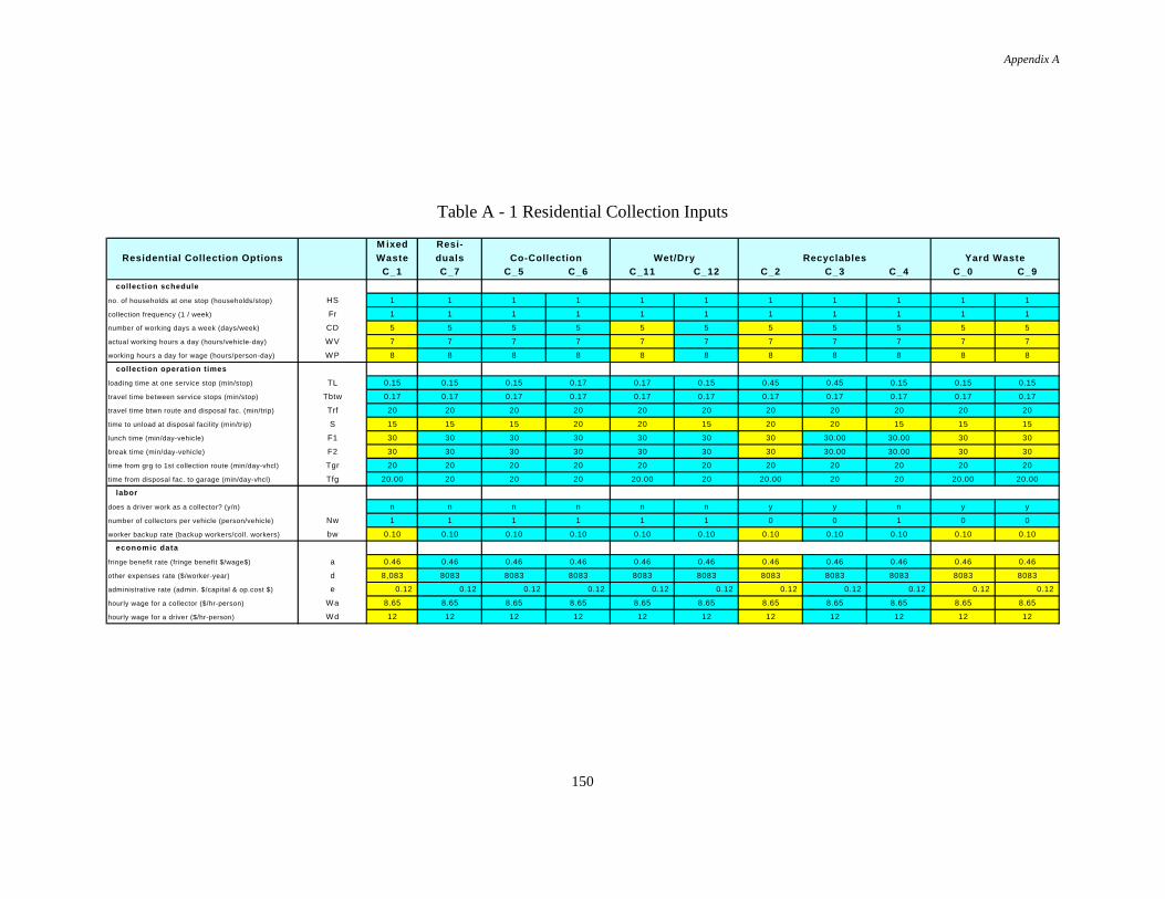
Appendix A
150
Table A - 1 Residential Collection Inputs
M ixed Resi-
Residential Collection Options Waste duals Co-Collection Wet/Dry RecyclablesC_1 C_7 C_5 C_6 C_11 C_12 C_2 C_3 C_4 C_0 C_9
collection schedule
no. of households at one stop (households/stop) HS 1 1 1 1 1 1 1 1 1 1 1
collection frequency (1 / week) Fr 1 1 1 1 1 1 1 1 1 1 1
number of working days a week (days/week) CD 5 5 5 5 5 5 5 5 5 5 5
actual working hours a day (hours/vehicle-day) WV 7 7 7 7 7 7 7 7 7 7 7
working hours a day for wage (hours/person-day) WP 8 8 8 8 8 8 8 8 8 8 8
collection operation times
loading time at one service stop (min/stop) TL 0.15 0.15 0.15 0.17 0.17 0.15 0.45 0.45 0.15 0.15 0.15
travel time between service stops (min/stop) Tbtw 0.17 0.17 0.17 0.17 0.17 0.17 0.17 0.17 0.17 0.17 0.17
travel time btwn route and disposal fac. (min/trip) Trf 20 20 20 20 20 20 20 20 20 20 20
time to unload at disposal facility (min/trip) S 15 15 15 20 20 15 20 20 15 15 15
lunch time (min/day-vehicle) F1 30 30 30 30 30 30 30 30.00 30.00 30 30
break time (min/day-vehicle) F2 30 30 30 30 30 30 30 30.00 30.00 30 30
time from grg to 1st collection route (min/day-vhcl) Tgr 20 20 20 20 20 20 20 20 20 20 20
time from disposal fac. to garage (min/day-vhcl) Tfg 20.00 20 20 20 20.00 20 20.00 20 20 20.00 20.00
labor
does a driver work as a collector? (y/n) n n n n n n y y n y y
number of collectors per vehicle (person/vehicle) Nw 1 1 1 1 1 1 0 0 1 0 0
worker backup rate (backup workers/coll. workers) bw 0.10 0.10 0.10 0.10 0.10 0.10 0.10 0.10 0.10 0.10 0.10
economic data
fringe benefit rate (fringe benefit $/wage$) a 0.46 0.46 0.46 0.46 0.46 0.46 0.46 0.46 0.46 0.46 0.46
other expenses rate ($/worker-year) d 8,083 8083 8083 8083 8083 8083 8083 8083 8083 8083 8083
administrative rate (admin. $/capital & op.cost $) e 0.12 0.12 0.12 0.12 0.12 0.12 0.12 0.12 0.12 0.12 0.12
hourly wage for a collector ($/hr-person) Wa 8.65 8.65 8.65 8.65 8.65 8.65 8.65 8.65 8.65 8.65 8.65
hourly wage for a driver ($/hr-person) Wd 12 12 12 12 12 12 12 12 12 12 12
Yard Waste

Appendix A
151
Table A - 2 Residential Collection Inputs (Continued)
M ixed Resi-Residential Collection Options Waste duals Co-Collection Wet/Dry Recyclables
C_1 C_7 C_5 C_6 C_11 C_12 C_2 C_3 C_4 C_0 C_9
collection vehicle
backup rate for vehicles (backup vhcl/coll. vhcl) bv 0.10 0.10 0.10 0.10 0.10 0.10 0.10 0.10 0.10 0.10 0.10
utilization factor (occupied yd3 / usable yd3) Ut 0.80 0.80 0.80 0.80 0.80 0.80 0.80 0.80 0.80 0.80 0.80
usable vehicle capacity (yd3) Vt 20 20 20 20 20 20 23 23 23 20 20
economic life of a vehicle (year) Lt 7 7 7 7 7 7 8 8 8 7 7
unit price of a vehicle ($/vehicle) Pt 133525.11 133525.1142 133525.1142 144652.207 144652.207 133525.1142 55635.46423 55635.46423 133525.1142 133525.1142 166906.3927
vehicle operation and maint. cost ($/vehicle) c 29375.53 29375.52511 29375.52511 33381.27854 33381.27854 29375.52511 30822.04718 30822.04718 29375.52511 29375.52511 29375.52511
msw compartment compaction density (lb / yd3) d_msw 0 N/A 0 0 N/A N/A N/A N/A N/A N/A N/A
recyclables compartment density (lb / yd3) d_recyc N/A N/A N/A 0 0 N/A 0 0 0 N/A N/A
residual waste compaction density (lb / yd3) d_residual N/A 0 N/A N/A N/A N/A N/A N/A N/A N/A N/A
wet waste compaction density (lb/yd3) d_wet N/A N/A N/A N/A 0 0 N/A N/A N/A N/A N/A
dry waste compaction density (lb/yd3) d_dry N/A N/A N/A N/A 0 0 N/A N/A N/A N/A N/A
yard waste compaction density (lb / yd3) d_yw N/A N/A N/A N/A N/A N/A N/A N/A N/A 0 0
travel speeds
between collection stops (miles/hour) Vbet 5 5 5 5 5 5 5 5 5 5 5
from collection route to facility (miles/hour) Vrf 30.00 30 30 30 30 30 30 30 30 30 30
from garage to route in the morning (mile/hour) Vgr 35 35 35 35 35 35 35 35 35 35 35
from facility to garage (miles/hour) Vfg 35 35 35 35 35 35 35 35 35 35 35
distances
distance between collection stops (miles) Dbet 0.0142 0.0142 0.0142 0.0142 0.0142 0.0142 0.0142 0.0142 0.0142 0.0142 0.0142
distance btwn collection route and facility (miles) Drf 11.00 11.00 11.00 11.00 15.00 15.00 11.00 11.00 11.00 10.00 10.00
distance btwn garage and collection route (miles) Dgr 11.667 11.667 11.667 11.667 11.667 11.667 11.667 11.667 11.667 11.667 11.667
distance between facility and garage (miles) Dfg 13.00 13.00 13.00 13.00 14.00 14.00 13.00 13.00 13.00 11.67 11.67
fuel usage rates
while traveling (m iles/gallon) MPG_trav_cv 5 5 5 5 5 5 5 5 5 5 5
between collection stops (miles/gallon) MPG_btwn_cv 2 2 2 2 2 2 2 2 2 2 2
while idling (gallons/hour) GPH_idle_cv 1 1 1 1 1 1 1 1 1 1 1
Yard Waste
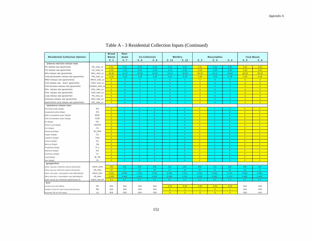
Appendix A
152
Table A - 3 Residential Collection Inputs (Continued)
M ixed Resi-
Residential Collection Options Waste duals Co-Collection Wet/Dry Recyclables
C_1 C_7 C_5 C_6 C_11 C_12 C_2 C_3 C_4 C_0 C_9
airborne emission release rates
HC release rate (gram/mile) HC_mile_cv 0.61 0.61 0.61 0.61 0.61 0.61 0.61 0.61 0.61 0.61 0.61
CO release rate (gram/mile) CO_mile_cv 5.03 5.03 5.03 5.03 5.03 5.03 5.03 5.03 5.03 5.03 5.03
NOx release rate (gram/mile) NOx_mile_cv 34.02 34.02 34.02 34.02 34.02 34.02 34.02 34.02 34.02 34.02 34.02
Total particulates release rate (gram/mile) PM_mile_cv 0.25 0.25 0.25 0.25 0.25 0.25 0.25 0.25 0.25 0.25 0.25
PM10 release rate (grams/mile) PM10_mile_cv 0 0 0 0 0 0 0 0 0 0 0
CO2 release rate - fossil (gram/mile) CO2f_mile_cv 0 0 0 0 0 0 0 0 0 0 0
CO2-biomass release rate (gram/mile) CO2bm_mile_cv 0 0 0 0 0 0 0 0 0 0 0
SOx release rate (gram/mile) SOx_mile_cv 0 0 0 0 0 0 0 0 0 0 0
CH4 release rate (gram/mile) CH4_mile_cv 0 0 0 0 0 0 0 0 0 0 0
Lead release rate (gram/mile) Pb_mile_cv 0 0 0 0 0 0 0 0 0 0 0
Ammonia release rate (gram/mile) NH3_mile_cv 0 0 0 0 0 0 0 0 0 0 0
Hydrochloric acid release rate (gram/mile) HCl_mile_cv 0 0 0 0 0 0 0 0 0 0 0
waterborne release rates
Dissolved solids (lb/gal) DS 0 0 0 0 0 0 0 0 0 0 0
Suspended solids (lb/gal) SS 0 0 0 0 0 0 0 0 0 0 0
BOD of washdown water (lb/gal) BOD 0 0 0 0 0 0 0 0 0 0 0
COD of washdown water (lb/gal) COD 0 0 0 0 0 0 0 0 0 0 0
Oil (lb/gal) OIL 0 0 0 0 0 0 0 0 0 0 0
Sulfuric acid (lb/gal) H2SO4 0 0 0 0 0 0 0 0 0 0 0
Iron (lb/gal) Fe 0 0 0 0 0 0 0 0 0 0 0
Ammonia (lb/gal) W _NH3 0 0 0 0 0 0 0 0 0 0 0
Copper (lb/gal) Cu 0 0 0 0 0 0 0 0 0 0 0
Cadmium (lb/gal) Cad 0 0 0 0 0 0 0 0 0 0 0
Arsenic (lb/gal) As 0 0 0 0 0 0 0 0 0 0 0
Mercury (lb/gal) Hg 0 0 0 0 0 0 0 0 0 0 0
Phosphate (lb/gal) P_x 0 0 0 0 0 0 0 0 0 0 0
Selenium (lb/gal) Se 0 0 0 0 0 0 0 0 0 0 0
Chromium (lb/gal) Cr 0 0 0 0 0 0 0 0 0 0 0
Lead (lb/gal) W _Pb 0 0 0 0 0 0 0 0 0 0 0
Zinc (lb/gal) Zn 0 0 0 0 0 0 0 0 0 0 0
garage/office
maint. area per collection vehicle (sf/vehicle) maint_area 400 400 400 400 400 400 400 400 400 400 400
office area per collection vehicle (sf/vehicle) off_area 20 20 20 20 20 20 20 20 20 20 20
maint. area elec. consumption rate (kW h/day/sf) maint_elec 0.001 0.001 0.001 0.001 0.001 0.001 0.001 0.001 0.001 0.001 0.001
office area elec. consumption rate (kW h/day/sf) off_elec 0.002 0.002 0.002 0.002 0.002 0.002 0.002 0.002 0.002 0.002 0.002
water volume per washdown (gallons/day-sf) maint_wd_vol 0.2 0.2 0.2 0.2 0.2 0.2 0.2 0.2 0.2 0.2 0.2
bins
unit price of a bin ($/bin) Pb N/A N/A N/A N/A 6.00 6.00 6.00 6.00 6.00 N/A N/A
number of bins for each house (bins/house) Rb N/A N/A N/A N/A 2 1 1 5 1 N/A N/A
economic life of a bin (year) Lb N/A N/A N/A N/A 8 8 8 8 8 N/A N/A
Yard Waste

Appendix A
153
Table A - 4 Residential Drop Off Inputs
Recyc- Yard
Residential Drop-off Options labels Waste
C_8 C_10
number of houses at one service stop (houses/stop) 0 N/A N/A
collection frequency (1/week) 0 N/A N/A
number of working days a week (days/week) CD 5 N/A
actual working hours a day (hours/vehicle-day) WV 7 N/A
working hours a day for wage (hours/person-day) WP 8 N/A
loading time at one service stop (min/stop) TL 20 N/A
travel time between service stops (min/stop) 0 N/A N/A
travel time btwn route and disposal fac. (min/trip) Thf 20 N/A
time to unload at disposal facility (min/trip) S 15 N/A
lunch time (min/day-vehicle) F1 30 N/A
break time (min/day-vehicle) F2 30 N/A
time from grg to 1st collection route (min/day-vhcl) Tgr 20 N/A
time from disposal fac. to garage (min/day-vhcl) Tfg 20.00 N/A
does a driver work as a collector? (y/n) 0 y N/A
number of collectors per vehicle (person/vehicle) Nw 0 N/A
worker backup rate (backup workers/coll. workers) bw 0.10 N/A
economic data 0 0 0
fringe benefit rate (fringe benefit $/wage$) a 0.46 N/A
other expenses rate ($/worker-year) d 8083 N/A
administrative rate (admin. $/capital & op.cost $) e 0.12 N/A
hourly wage for a collector ($/hr-person) Wa 0.00 N/A
hourly wage for a driver ($/hr-person) Wd 12 N/A
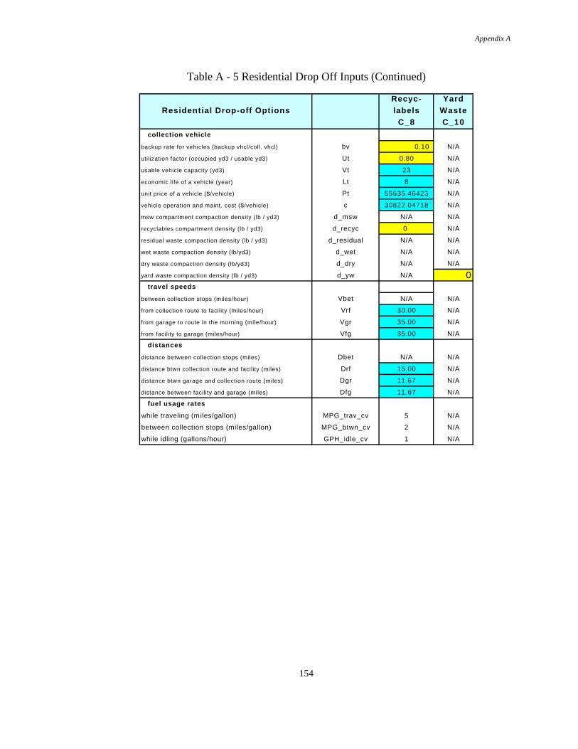
Appendix A
154
Table A - 5 Residential Drop Off Inputs (Continued)
Recyc- Yard
Residential Drop-off Options labels Waste
C_8 C_10
collection vehicle
backup rate for vehicles (backup vhcl/coll. vhcl) bv 0.10 N/A
utilization factor (occupied yd3 / usable yd3) Ut 0.80 N/A
usable vehicle capacity (yd3) Vt 23 N/A
economic life of a vehicle (year) Lt 8 N/A
unit price of a vehicle ($/vehicle) Pt 55635.46423 N/A
vehicle operation and maint. cost ($/vehicle) c 30822.04718 N/A
msw compartment compaction density (lb / yd3) d_msw N/A N/A
recyclables compartment density (lb / yd3) d_recyc 0 N/A
residual waste compaction density (lb / yd3) d_residual N/A N/A
wet waste compaction density (lb/yd3) d_wet N/A N/A
dry waste compaction density (lb/yd3) d_dry N/A N/A
yard waste compaction density (lb / yd3) d_yw N/A 0 travel speeds
between collection stops (miles/hour) Vbet N/A N/A
from collection route to facility (miles/hour) Vrf 30.00 N/A
from garage to route in the morning (mile/hour) Vgr 35.00 N/A
from facility to garage (miles/hour) Vfg 35.00 N/A
distances
distance between collection stops (miles) Dbet N/A N/A
distance btwn collection route and facility (miles) Drf 15.00 N/A
distance btwn garage and collection route (miles) Dgr 11.67 N/A
distance between facility and garage (miles) Dfg 11.67 N/A
fuel usage rates
while traveling (miles/gallon) MPG_trav_cv 5 N/A
between collection stops (miles/gallon) MPG_btwn_cv 2 N/A
while idling (gallons/hour) GPH_idle_cv 1 N/A

Appendix A
155
Table A - 6 Residential Drop Off Inputs (Continued)
Recyc- Yard
Residential Drop-off Options labels Waste
C_8 C_10
airborne emission release rates
HC release rate (gram/mile) HC_mile_cv 0.61 N/A
CO release rate (gram/mile) CO_mile_cv 5.03 N/A
NOx release rate (gram/mile) NOx_mile_cv 34.02 N/A
Total particulates release rate (gram/mile) PM_mile_cv 0.25 N/A
PM10 release rate (grams/mile) PM10_mile_cv 0 N/A
CO2 release rate - fossil (gram/mile) CO2f_mile_cv 0 N/A
CO2-biomass release rate (gram/mile) CO2bm_mile_cv 0 N/A
SOx release rate (gram/mile) SOx_mile_cv 0 N/A
CH4 release rate (gram/mile) CH4_mile_cv 0 N/A
Lead release rate (gram/mile) Pb_mile_cv 0 N/A
Ammonia release rate (gram/mile) NH3_mile_cv 0 N/A
Hydrochloric acid release rate (gram/mile) HCl_mile_cv 0 N/A
waterborne release rates
Dissolved solids (lb/gal) DS 0 N/A
Suspended solids (lb/gal) SS 0 N/A
BOD of washdown water (lb/gal) BOD 0 N/A
COD of washdown water (lb/gal) COD 0 N/A
Oil (lb/gal) OIL 0 N/A
Sulfuric acid (lb/gal) H2SO4 0 N/A
Iron (lb/gal) Fe 0 N/A
Ammonia (lb/gal) W_NH3 0 N/A
Copper (lb/gal) Cu 0 N/A
Cadmium (lb/gal) Cad 0 N/A
Arsenic (lb/gal) As 0 N/A
Mercury (lb/gal) Hg 0 N/A
Phosphate (lb/gal) P_x 0 N/A
Selenium (lb/gal) Se 0 N/A
Chromium (lb/gal) Cr 0 N/A
Lead (lb/gal) W_Pb 0 N/A
Zinc (lb/gal) Zn 0 N/A
garage/office
maint. area per collection vehicle (sf/vehicle) maint_area 400 N/A
office area per collection vehicle (sf/vehicle) off_area 20 N/A
maint. area elec. consumption rate (kW h/day/sf) maint_elec 0.001 N/A
office area elec. consumption rate (kW h/day/sf) off_elec 0.002 N/A
water volume per washdown (gallons/day-sf) maint_wd_vol 0.2 N/A
bins
Pb N/A N/A
number of bins for each house (bins/house) Rb N/A N/A
economic life of a bin (year) Lb N/A N/A
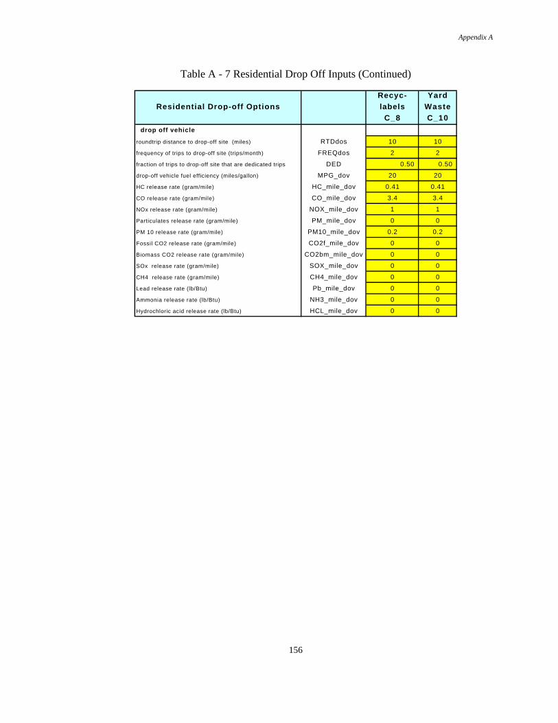
Appendix A
156
Table A - 7 Residential Drop Off Inputs (Continued)
Recyc- Yard
Residential Drop-off Options labels Waste
C_8 C_10
drop off vehicle
roundtrip distance to drop-off site (miles) RTDdos 10 10
frequency of trips to drop-off site (trips/month) FREQdos 2 2
fraction of trips to drop-off site that are dedicated trips DED 0.50 0.50
drop-off vehicle fuel efficiency (miles/gallon) MPG_dov 20 20
HC release rate (gram/mile) HC_mile_dov 0.41 0.41
CO release rate (gram/mile) CO_mile_dov 3.4 3.4
NOx release rate (gram/mile) NOX_mile_dov 1 1
Particulates release rate (gram/mile) PM_mile_dov 0 0
PM 10 release rate (gram/mile) PM10_mile_dov 0.2 0.2
Fossil CO2 release rate (gram/mile) CO2f_mile_dov 0 0
Biomass CO2 release rate (gram/mile) CO2bm_mile_dov 0 0
SOx release rate (gram/mile) SOX_mile_dov 0 0
CH4 release rate (gram/mile) CH4_mile_dov 0 0
Lead release rate (lb/Btu) Pb_mile_dov 0 0
Ammonia release rate (lb/Btu) NH3_mile_dov 0 0
Hydrochloric acid release rate (lb/Btu) HCL_mile_dov 0 0

Appendix A
157
Table A - 8 Multi-Family Collection Inputs
M ixed Resi- Recyclables
Multi-Fam ily Collection Options Waste duals Wet/Dry
C_13 C_16 C_17 C_18 C_14 C_15
collection schedule
collection frequency (1 / week) Fr 1 1 1 1 1 1
number of working days a week (days/week) CD 5 5 5 5 5 5
actual working hours a day (hours/vehicle-day) WV 7 7 7 7 7 7
working hours a day for wage (hours/person-day) WP 8 8 8 8 8 8
loading time at one service stop (min/stop) TL 5 5 5 5 10 10
travel time between service stops (min/stop) Tbet 1.5 1.5 1.5 1.5 1.5 1.5
travel time btwn route and disposal fac. (min/trip) Thf 20 20 20.00 20 20 20
time to unload at disposal facility (min/trip) S 15 15 20 15 20 15
lunch time (min/day-vehicle) F1 30 30 30 30 30 30
break time (min/day-vehicle) F2 30 30 30 30 30 30
time from grg to 1st collection route (min/day-vhcl) Tgr 20 20 20 20 20 20
time from disposal fac. to garage (min/day-vhcl) Tfg 20.00 20 20.00 20 20 20
does a driver work as a collector? (y/n) 0 n n n n y n
number of collectors per vehicle (person/vehicle) Nw 1 1 1 1 0 1
worker backup rate (backup workers/coll. workers) bw 0.10 0.10 0.10 0.10 0.10 0.10
economic data
fringe benefit rate (fringe benefit $/wage$) a 0.46 0.46 0.46 0.46 0.46 0.46
other expenses rate ($/worker-year) d 8083 8083 8083 8083 8083 8083
administrative rate (admin. $/capital & op.cost $) e 0.12 0.12 0.12 0.12 0.12 0.12
hourly wage for a collector ($/hr-person) Wa 8.65 8.65 8.65 8.65 8.65 8.65
hourly wage for a driver ($/hr-person) Wd 12 12 12 12 12 12
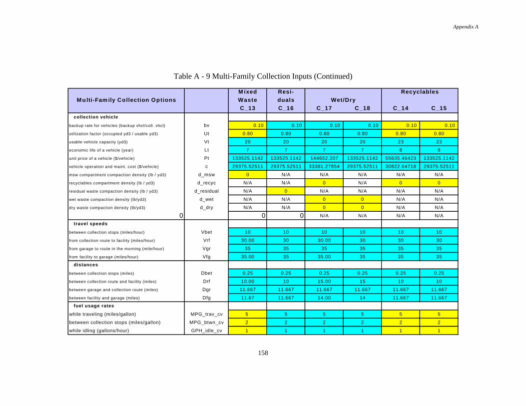
Appendix A
158
Table A - 9 Multi-Family Collection Inputs (Continued)
M ixed Resi- Recyclables
Multi-Fam ily Collection Options Waste duals Wet/Dry
C_13 C_16 C_17 C_18 C_14 C_15
collection vehicle
backup rate for vehicles (backup vhcl/coll. vhcl) bv 0.10 0.10 0.10 0.10 0.10 0.10
utilization factor (occupied yd3 / usable yd3) Ut 0.80 0.80 0.80 0.80 0.80 0.80
usable vehicle capacity (yd3) Vt 20 20 20 20 23 23
economic life of a vehicle (year) Lt 7 7 7 7 8 8
unit price of a vehicle ($/vehicle) Pt 133525.1142 133525.1142 144652.207 133525.1142 55635.46423 133525.1142
vehicle operation and maint. cost ($/vehicle) c 29375.52511 29375.52511 33381.27854 29375.52511 30822.04718 29375.52511
msw compartment compaction density (lb / yd3) d_msw 0 N/A N/A N/A N/A N/A
recyclables compartment density (lb / yd3) d_recyc N/A N/A 0 N/A 0 0
residual waste compaction density (lb / yd3) d_residual N/A 0 N/A N/A N/A N/A
wet waste compaction density (lb/yd3) d_wet N/A N/A 0 0 N/A N/A
dry waste compaction density (lb/yd3) d_dry N/A N/A 0 0 N/A N/A
0 0 0 N/A N/A N/A N/A
travel speeds
between collection stops (miles/hour) Vbet 10 10 10 10 10 10
from collection route to facility (miles/hour) Vrf 30.00 30 30.00 30 30 30
from garage to route in the morning (mile/hour) Vgr 35 35 35 35 35 35
from facility to garage (miles/hour) Vfg 35.00 35 35.00 35 35 35
distances
between collection stops (miles) Dbet 0.25 0.25 0.25 0.25 0.25 0.25
between collection route and facility (miles) Drf 10.00 10 15.00 15 10 10
between garage and collection route (miles) Dgr 11.667 11.667 11.667 11.667 11.667 11.667
between facility and garage (miles) Dfg 11.67 11.667 14.00 14 11.667 11.667
fuel usage rates
while traveling (miles/gallon) MPG_trav_cv 5 5 5 5 5 5
between collection stops (miles/gallon) MPG_btwn_cv 2 2 2 2 2 2
while idling (gallons/hour) GPH_idle_cv 1 1 1 1 1 1
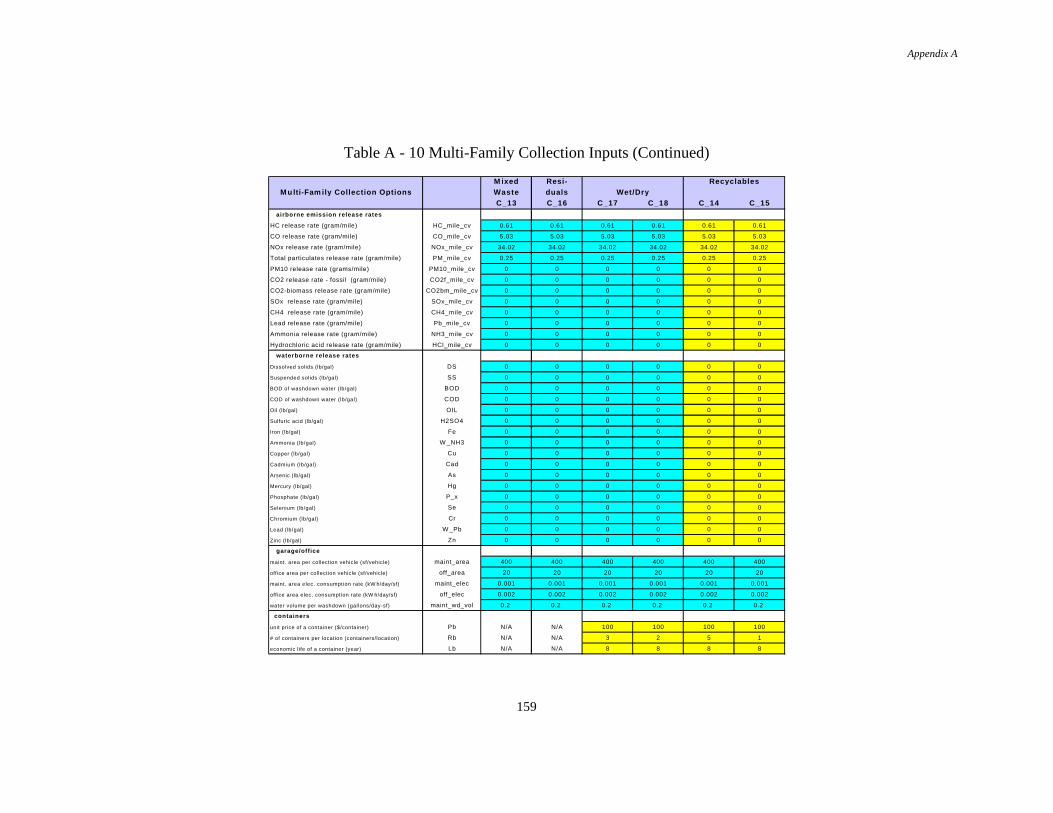
Appendix A
159
Table A - 10 Multi-Family Collection Inputs (Continued)
M ixed Resi- Recyclables
M u lti-Fam ily Collection Options Waste duals Wet/Dry
C_13 C_16 C_17 C_18 C_14 C_15
airborne emission release rates
HC release rate (gram/mile) HC_mile_cv 0.61 0.61 0.61 0.61 0.61 0.61
CO release rate (gram/mile) CO_mile_cv 5.03 5.03 5.03 5.03 5.03 5.03
NOx release rate (gram/mile) NOx_mile_cv 34.02 34.02 34.02 34.02 34.02 34.02
Total particulates release rate (gram/mile) PM_mile_cv 0.25 0.25 0.25 0.25 0.25 0.25
PM10 release rate (grams/mile) PM10_mile_cv 0 0 0 0 0 0
CO2 release rate - fossil (gram/mile) CO2f_mile_cv 0 0 0 0 0 0
CO2-biomass release rate (gram/mile) CO2bm_mile_cv 0 0 0 0 0 0
SOx release rate (gram/mile) SOx_mile_cv 0 0 0 0 0 0
CH4 release rate (gram/mile) CH4_mile_cv 0 0 0 0 0 0
Lead release rate (gram/mile) Pb_mile_cv 0 0 0 0 0 0
Ammonia release rate (gram/mile) NH3_mile_cv 0 0 0 0 0 0
Hydrochloric acid release rate (gram/mile) HCl_mile_cv 0 0 0 0 0 0
waterborne release rates
Dissolved solids (lb/gal) DS 0 0 0 0 0 0
Suspended solids (lb/gal) SS 0 0 0 0 0 0
BOD of washdown water (lb/gal) BOD 0 0 0 0 0 0
COD of washdown water (lb/gal) COD 0 0 0 0 0 0
Oil (lb/gal) OIL 0 0 0 0 0 0
Sulfuric acid (lb/gal) H2SO4 0 0 0 0 0 0
Iron (lb/gal) Fe 0 0 0 0 0 0
Ammonia (lb/gal) W _NH3 0 0 0 0 0 0
Copper (lb/gal) Cu 0 0 0 0 0 0
Cadmium (lb/gal) Cad 0 0 0 0 0 0
Arsenic (lb/gal) As 0 0 0 0 0 0
Mercury (lb/gal) Hg 0 0 0 0 0 0
Phosphate (lb/gal) P_x 0 0 0 0 0 0
Selenium (lb/gal) Se 0 0 0 0 0 0
Chromium (lb/gal) Cr 0 0 0 0 0 0
Lead (lb/gal) W _Pb 0 0 0 0 0 0
Zinc (lb/gal) Zn 0 0 0 0 0 0
garage/office
maint. area per collection vehicle (sf/vehicle) maint_area 400 400 400 400 400 400
office area per collection vehicle (sf/vehicle) off_area 20 20 20 20 20 20
maint. area elec. consumption rate (kW h/day/sf) maint_elec 0.001 0.001 0.001 0.001 0.001 0.001
office area elec. consumption rate (kW h/day/sf) off_elec 0.002 0.002 0.002 0.002 0.002 0.002
water volume per washdown (gallons/day-sf) maint_wd_vol 0.2 0.2 0.2 0.2 0.2 0.2
containers
unit price of a container ($/container) Pb N/A N/A 100 100 100 100
# of containers per location (containers/location) Rb N/A N/A 3 2 5 1
economic life of a container (year) Lb N/A N/A 8 8 8 8
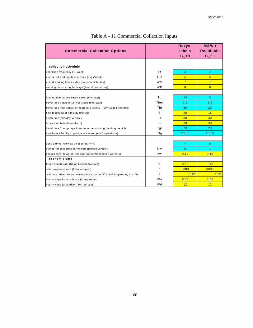
Appendix A
160
Table A - 11 Commercial Collection Inputs
Recyc- M S W /
Commercial Collection Options labels Residuals
C_19 C_20
collection schedule
collection frequency (1 / week) Fr 3 2
number of working days a week (days/week) CD 5 5
actual working hours a day (hours/vehicle-day) WV 7 7
working hours a day for wage (hours/person-day) WP 8 8
loading time at one service stop (min/stop) TL 10 5
travel time between service stops (min/stop) Tbet 1.5 1.5
travel time from collection route to a facility - fully loaded (min/trip) Thf 20 20
time to unload at a facility (min/trip) S 20 15
lunch time (min/day-vehicle) F1 30 30
break time (min/day-vehicle) F2 30 30
travel time from garage to route in the morning (min/day-vehicle) Tgr 20 20
time from a facility to garage at the end (min/day-vehicle) Tfg 20.00 20.00
does a driver work as a collector? (y/n) y n
number of collectors per vehicle (person/vehicle) Nw 0 1
backup rate for worker (backup workers/collection workers) bw 0.10 0.10
economic data
fringe benefit rate (fringe benefit $/wage$) a 0.46 0.46
other expenses rate ($/worker-year) d 8083 8083
administrative rate (administrative expense $/capital & operating cost $) e 0.12 0.12
hourly wage for a collector ($/hr-person) Wa 8.65 8.65
hourly wage for a driver ($/hr-person) Wd 12 12
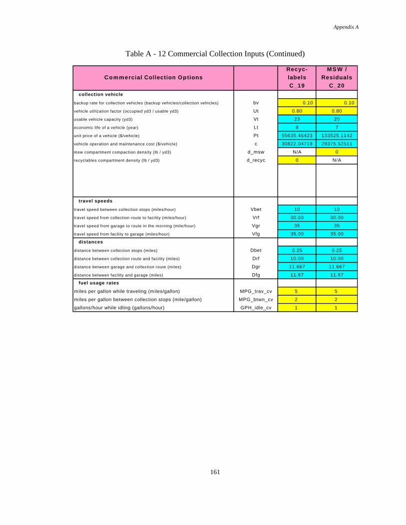
Appendix A
161
Table A - 12 Commercial Collection Inputs (Continued)
Recyc- M S W /
Commercial Collection Options labels Residuals
C_19 C_20
collection vehicle
backup rate for collection vehicles (backup vehicles/collection vehicles) bv 0.10 0.10
vehicle utilization factor (occupied yd3 / usable yd3) Ut 0.80 0.80
usable vehicle capacity (yd3) Vt 23 20
economic life of a vehicle (year) Lt 8 7
unit price of a vehicle ($/vehicle) Pt 55635.46423 133525.1142
vehicle operation and maintenance cost ($/vehicle) c 30822.04718 29375.52511
msw compartment compaction density (lb / yd3) d_msw N/A 0
recyclables compartment density (lb / yd3) d_recyc 0 N/A
travel speeds
travel speed between collection stops (miles/hour) Vbet 10 10
travel speed from collection route to facility (miles/hour) Vrf 30.00 30.00
travel speed from garage to route in the morning (mile/hour) Vgr 35 35
travel speed from facility to garage (miles/hour) Vfg 35.00 35.00
distances
distance between collection stops (miles) Dbet 0.25 0.25
distance between collection route and facility (miles) Drf 10.00 10.00
distance between garage and collection route (miles) Dgr 11.667 11.667
distance between facility and garage (miles) Dfg 11.67 11.67
fuel usage rates
miles per gallon while traveling (miles/gallon) MPG_trav_cv 5 5
miles per gallon between collection stops (mile/gallon) MPG_btwn_cv 2 2
gallons/hour while idling (gallons/hour) GPH_idle_cv 1 1

Appendix A
162
Table A - 13 Commercial Collection Inputs (Continued)
Recyc- M S W /
Commercial Collection Options labels Residuals
C_19 C_20
airborne emission release rates
HC release rate (gram/mile) HC_mile_cv 0.61 0.61
CO release rate (gram/mile) CO_mile_cv 5.03 5.03
NOx release rate (gram/mile) NOx_mile_cv 34.02 34.02
Total particulates release rate (gram/mile) PM_mile_cv 0.25 0.25
PM10 release rate (grams/mile) PM10_mile_cv 0 0
CO2 release rate - fossil (gram/mile) CO2f_mile_cv 0 0
CO2-biomass release rate (gram/mile) CO2bm_mile_cv 0 0
SOx release rate (gram/mile) SOx_mile_cv 0 0
CH4 release rate (gram/mile) CH4_mile_cv 0 0
Lead release rate (gram/mile) Pb_mile_cv 0 0
Ammonia release rate (gram/mile) NH3_mile_cv 0 0
Hydrochloric acid release rate (gram/mile) HCl_mile_cv 0 0
waterborne release rates
Dissolved solids (lb/gal) DS 0 0
Suspended solids (lb/gal) SS 0 0
BOD of washdown water (lb/gal) BOD 0 0
COD of washdown water (lb/gal) COD 0 0
Oil (lb/gal) OIL 0 0
Sulfuric acid (lb/gal) H2SO4 0 0
Iron (lb/gal) Fe 0 0
Ammonia (lb/gal) W_NH3 0 0
Copper (lb/gal) Cu 0 0
Cadmium (lb/gal) Cad 0 0
Arsenic (lb/gal) As 0 0
Mercury (lb/gal) Hg 0 0
Phosphate (lb/gal) P_x 0 0
Selenium (lb/gal) Se 0 0
Chromium (lb/gal) Cr 0 0
Lead (lb/gal) W_Pb 0 0
Zinc (lb/gal) Zn 0 0
garage/office
maintenance area per collection vehicle (sf/vehicle) maint_area 400 400
office area per collection vehicle (sf/vehicle) off_area 20 20
maintenance area daily electricity consumption rate (kW h/day/sf) maint_elec 0.001 0.001
office area daily electricity consumption rate (kW h/day/sf) off_elec 0.002 0.002
water volume per washdown (gallons/day-sf) maint_wd_vol 0.2 0.2
containers
unit price of a container ($/container) Pb N/A N/A
number of containers at each location (containers/location) Rb 5 N/A
economic life of a container (year) Lb N/A N/A

Appendix A
163
Table A - 14 Residential Capture Rates
Mixed W aste Residuals Co-Collection
DESCRIPTION VARIABLE NAME C 1 C 7 C 5 C 6
Sector 1 Sector 2
Selected Sector Sector 1 Sector 2
Selected Sector Sector 1 Sector 2
Selected Sector Sector 1 Sector 2
Selected Sector
R_CR_TABLE C_1_CR_1 C_1_CR_2 C_1_CR C_7_CR_1 C_7_CR_2 C_7_CR C_5_CR_1 C_5_CR_2 C_5_CR C_6_CR_1 C_6_CR_2 C_6_CR
Yard Trimmings, Leaves R_YTL 1.00 1.00 1.00 1.00 1.00 1.00
Yard Trimmings, Grass R_YTG 1.00 1.00 1.00 1.00 1.00 1.00
Yard Trimmings, Branches R_YTB 1.00 1.00 1.00 1.00 1.00 1.00
Old News Print R_ONP 1.00 1.00 1.00 1.00 1.00 1.00 0.68 0.67 0.68 0.68 0.67 0.68
Old Corr. Cardboard R_OCC 1.00 1.00 1.00 1.00 1.00 1.00 0.56 0.55 0.56 0.56 0.55 0.56
Office Paper R_OFF 1.00 1.00 1.00 1.00 1.00 1.00 0.49 0.48 0.49 0.49 0.48 0.49
Phone Books R_PBK 1.00 1.00 1.00 1.00 1.00 1.00 0.60 0.59 0.60 0.60 0.59 0.60
Books R_BOOK 1.00 1.00 1.00 1.00 1.00 1.00 0.60 0.59 0.60 0.60 0.59 0.60
Old Magazines R_OMG 1.00 1.00 1.00 1.00 1.00 1.00 0.60 0.59 0.60 0.60 0.59 0.60
3rd Class Mail R_MAIL 1.00 1.00 1.00 1.00 1.00 1.00 0.60 0.59 0.60 0.60 0.59 0.60
Paper Other #1 R_PAOT1 1.00 1.00 1.00 1.00 1.00 1.00 0.60 0.59 0.60 0.60 0.59 0.60
Paper Other #2 R_PAOT2 1.00 1.00 1.00 1.00 1.00 1.00 0.60 0.59 0.60 0.60 0.59 0.60
Paper Other #3 R_PAOT3 1.00 1.00 1.00 1.00 1.00 1.00 0.60 0.59 0.60 0.60 0.59 0.60
Paper Other #4 R_PAOT4 1.00 1.00 1.00 1.00 1.00 1.00 0.60 0.59 0.60 0.60 0.59 0.60
Paper Other #5 R_PAOT5 1.00 1.00 1.00 1.00 1.00 1.00 0.60 0.59 0.60 0.60 0.59 0.60
CCCR Other R_CCR_O 1.00 1.00 1.00 1.00 1.00 1.00 0.60 0.59 0.60 0.60 0.59 0.60
Mixed Paper R_PMIX 1.00 1.00 1.00 1.00 1.00 1.00 0.60 0.59 0.60 0.60 0.59 0.60
HDPE - Translucent R_HDT 1.00 1.00 1.00 1.00 1.00 1.00 0.56 0.55 0.56 0.56 0.55 0.56
HDPE - Pigmented R_HDP 1.00 1.00 1.00 1.00 1.00 1.00 0.56 0.55 0.56 0.56 0.55 0.56
PET R_PPET 1.00 1.00 1.00 1.00 1.00 1.00 0.56 0.55 0.56 0.56 0.55 0.56
Plastic - Other #1 R_PLOT1 1.00 1.00 1.00 1.00 1.00 1.00 0.56 0.55 0.56 0.56 0.55 0.56
Plastic - Other #2 R_PLOT2 1.00 1.00 1.00 1.00 1.00 1.00 0.56 0.55 0.56 0.56 0.55 0.56
Plastic - Other #3 R_PLOT3 1.00 1.00 1.00 1.00 1.00 1.00 0.56 0.55 0.56 0.56 0.55 0.56
Plastic - Other #4 R_PLOT4 1.00 1.00 1.00 1.00 1.00 1.00 0.56 0.55 0.56 0.56 0.55 0.56
Plastic - Other #5 R_PLOT5 1.00 1.00 1.00 1.00 1.00 1.00 0.56 0.55 0.56 0.56 0.55 0.56
Mixed Plastic R_PLMIX 1.00 1.00 1.00 1.00 1.00 1.00 0.56 0.55 0.56 0.56 0.55 0.56
CCNR Other R_CNR_O 1.00 1.00 1.00 1.00 1.00 1.00
Ferrous Cans R_FCAN 1.00 1.00 1.00 1.00 1.00 1.00 0.58 0.57 0.58 0.58 0.57 0.58
Ferrous Metal - Other R_FMOT 1.00 1.00 1.00 1.00 1.00 1.00 0.58 0.57 0.58 0.58 0.57 0.58
Aluminum Cans R_ACAN 1.00 1.00 1.00 1.00 1.00 1.00 0.64 0.63 0.64 0.64 0.63 0.64
Aluminum - Other #1 R_ALOT1 1.00 1.00 1.00 1.00 1.00 1.00 0.64 0.63 0.64 0.64 0.63 0.64
Aluminum - Other #2 R_ALOT2 1.00 1.00 1.00 1.00 1.00 1.00 0.64 0.63 0.64 0.64 0.63 0.64
Glass - Clear R_GCLR 1.00 1.00 1.00 1.00 1.00 1.00 0.64 0.63 0.64 0.64 0.63 0.64
Glass - Brown R_GBRN 1.00 1.00 1.00 1.00 1.00 1.00 0.64 0.63 0.64 0.64 0.63 0.64
Glass - Green R_GGRN 1.00 1.00 1.00 1.00 1.00 1.00 0.64 0.63 0.64 0.64 0.63 0.64
Mixed Glass R_GMIX 1.00 1.00 1.00 1.00 1.00 1.00 0.64 0.63 0.64 0.64 0.63 0.64
CNNR Other R_NNR_O 1.00 1.00 1.00 1.00 1.00 1.00
Paper - Non-recyclable R_PANR 1.00 1.00 1.00 1.00 1.00 1.00
Food W aste R_FW 1.00 1.00 1.00 1.00 1.00 1.00
CCCN Other R_CCN_O 1.00 1.00 1.00 1.00 1.00 1.00
Plastic - Non-Recyclable R_PLNR 1.00 1.00 1.00 1.00 1.00 1.00
Misc. R_MIS_CNN 1.00 1.00 1.00 1.00 1.00 1.00
CCNN Other R_CNN_O 1.00 1.00 1.00 1.00 1.00 1.00
Ferrous - Non-recyclable R_FNR 1.00 1.00 1.00 1.00 1.00 1.00
Al - Non-recyclable R_ANR 1.00 1.00 1.00 1.00 1.00 1.00
Glass - Non-recyclable R_GNR 1.00 1.00 1.00 1.00 1.00 1.00
Misc. R_MIS_NNN 1.00 1.00 1.00 1.00 1.00 1.00
CNNN Other R_NNN_O 1.00 1.00 1.00 1.00 1.00 1.00
Participation Factor R_PF 1.0 1.0 1.0 1.0 1.0 1.0 1.0 1.0 1.0 1.0 1.0 1.0
RESIDENTIAL COLLECTION OPTIONS

Appendix A
164
Table A - 15 Residential Capture Rates (Continued)
Wet/Dry Recyclables
DESCRIPTION VARIABLE NAME C 11 C 12 C 2 C 3
Sector 1 Sector 2
Selected
Sector Sector 1 Sector 2
Selected
Sector Sector 1 Sector 2
Selected
Sector Sector 1 Sector 2
Selected
Sector Sector 1 Sector 2
Selected
Sector
R_CR_TABLE C_11_CR_1 C_11_CR_2 C_11_CR C_12_CR_1 C_12_CR_2 C_12_CR C_2_CR_1 C_2_CR_2 C_2_CR C_3_CR_1 C_3_CR_2 C_3_CR C_4_CR_1 C_4_CR_2 C_4_CR
Yard Trimmings, Leaves R_YTL 1.00 1.00 1.00 1.00 1.00 1.00
Yard Trimmings, Grass R_YTG 1.00 1.00 1.00 1.00 1.00 1.00
Yard Trimmings, Branches R_YTB 1.00 1.00 1.00 1.00 1.00 1.00
Old News Print R_ONP 1.00 1.00 1.00 1.00 1.00 1.00 0.68 0.67 0.68 0.63 0.62 0.63 0.68 0.67 0.68
Old Corr. Cardboard R_OCC 1.00 1.00 1.00 1.00 1.00 1.00 0.56 0.55 0.56 0.53 0.52 0.53 0.56 0.55 0.56
Office Paper R_OFF 1.00 1.00 1.00 1.00 1.00 1.00 0.49 0.48 0.49 0.46 0.46 0.46 0.49 0.48 0.49
Phone Books R_PBK 1.00 1.00 1.00 1.00 1.00 1.00 0.60 0.59 0.60 0.56 0.45 0.56 0.60 0.59 0.60
Books R_BOOK 1.00 1.00 1.00 1.00 1.00 1.00 0.60 0.59 0.60 0.56 0.55 0.56 0.60 0.59 0.60
Old Magazines R_OMG 1.00 1.00 1.00 1.00 1.00 1.00 0.60 0.59 0.60 0.56 0.55 0.56 0.60 0.59 0.60
3rd Class Mail R_MAIL 1.00 1.00 1.00 1.00 1.00 1.00 0.60 0.59 0.60 0.56 0.55 0.56 0.60 0.59 0.60
Paper Other #1 R_PAOT1 1.00 1.00 1.00 1.00 1.00 1.00 0.60 0.59 0.60 0.56 0.55 0.56 0.60 0.59 0.60
Paper Other #2 R_PAOT2 1.00 1.00 1.00 1.00 1.00 1.00 0.60 0.59 0.60 0.56 0.55 0.56 0.60 0.59 0.60
Paper Other #3 R_PAOT3 1.00 1.00 1.00 1.00 1.00 1.00 0.60 0.59 0.60 0.56 0.55 0.56 0.60 0.59 0.60
Paper Other #4 R_PAOT4 1.00 1.00 1.00 1.00 1.00 1.00 0.60 0.59 0.60 0.56 0.55 0.56 0.60 0.59 0.60
Paper Other #5 R_PAOT5 1.00 1.00 1.00 1.00 1.00 1.00 0.60 0.59 0.60 0.56 0.55 0.56 0.60 0.59 0.60
CCCR Other R_CCR_O 1.00 1.00 1.00 1.00 1.00 1.00 0.60 0.59 0.60 0.56 0.55 0.56 0.60 0.59 0.60
Mixed Paper R_PMIX 1.00 1.00 1.00 1.00 1.00 1.00 0.60 0.59 0.60 0.56 0.55 0.56 0.60 0.59 0.60
HDPE - Translucent R_HDT 1.00 1.00 1.00 1.00 1.00 1.00 0.56 0.55 0.56 0.53 0.52 0.53 0.56 0.55 0.56
HDPE - Pigmented R_HDP 1.00 1.00 1.00 1.00 1.00 1.00 0.56 0.55 0.56 0.53 0.52 0.53 0.56 0.55 0.56
PET R_PPET 1.00 1.00 1.00 1.00 1.00 1.00 0.56 0.55 0.56 0.53 0.52 0.53 0.56 0.55 0.56
Plastic - Other #1 R_PLOT1 1.00 1.00 1.00 1.00 1.00 1.00 0.56 0.55 0.56 0.53 0.52 0.53 0.56 0.55 0.56
Plastic - Other #2 R_PLOT2 1.00 1.00 1.00 1.00 1.00 1.00 0.56 0.55 0.56 0.53 0.52 0.53 0.56 0.55 0.56
Plastic - Other #3 R_PLOT3 1.00 1.00 1.00 1.00 1.00 1.00 0.56 0.55 0.56 0.53 0.52 0.53 0.56 0.55 0.56
Plastic - Other #4 R_PLOT4 1.00 1.00 1.00 1.00 1.00 1.00 0.56 0.55 0.56 0.53 0.52 0.53 0.56 0.55 0.56
Plastic - Other #5 R_PLOT5 1.00 1.00 1.00 1.00 1.00 1.00 0.56 0.55 0.56 0.53 0.52 0.53 0.56 0.55 0.56
Mixed Plastic R_PLMIX 1.00 1.00 1.00 1.00 1.00 1.00 0.56 0.55 0.56 0.53 0.52 0.53 0.56 0.55 0.56
CCNR Other R_CNR_O 1.00 1.00 1.00 1.00 1.00 1.00
Ferrous Cans R_FCAN 1.00 1.00 1.00 1.00 1.00 1.00 0.58 0.57 0.58 0.53 0.52 0.53 0.58 0.57 0.58
Ferrous Metal - Other R_FMOT 1.00 1.00 1.00 1.00 1.00 1.00 0.58 0.57 0.58 0.53 0.52 0.53 0.58 0.57 0.58
Aluminum Cans R_ACAN 1.00 1.00 1.00 1.00 1.00 1.00 0.64 0.63 0.64 0.60 0.59 0.60 0.64 0.63 0.64
Aluminum - Other #1 R_ALOT1 1.00 1.00 1.00 1.00 1.00 1.00 0.64 0.63 0.64 0.60 0.59 0.60 0.64 0.63 0.64
Aluminum - Other #2 R_ALOT2 1.00 1.00 1.00 1.00 1.00 1.00 0.64 0.63 0.64 0.60 0.59 0.60 0.64 0.63 0.64
Glass - Clear R_GCLR 1.00 1.00 1.00 1.00 1.00 1.00 0.64 0.63 0.64 0.60 0.59 0.60 0.64 0.63 0.64
Glass - Brown R_GBRN 1.00 1.00 1.00 1.00 1.00 1.00 0.64 0.63 0.64 0.60 0.59 0.60 0.64 0.63 0.64
Glass - Green R_GGRN 1.00 1.00 1.00 1.00 1.00 1.00 0.64 0.63 0.64 0.60 0.59 0.60 0.64 0.63 0.64
Mixed Glass R_GMIX 1.00 1.00 1.00 1.00 1.00 1.00 0.64 0.63 0.64 0.60 0.59 0.60 0.64 0.63 0.64
CNNR Other R_NNR_O 1.00 1.00 1.00 1.00 1.00 1.00
Paper - Non-recyclable R_PANR 1.00 1.00 1.00 1.00 1.00 1.00
Food Waste R_FW 1.00 1.00 1.00 1.00 1.00 1.00
CCCN Other R_CCN_O 1.00 1.00 1.00 1.00 1.00 1.00
Plastic - Non-Recyclable R_PLNR 1.00 1.00 1.00 1.00 1.00 1.00
Misc. R_MIS_CNN 1.00 1.00 1.00 1.00 1.00 1.00
CCNN Other R_CNN_O 1.00 1.00 1.00 1.00 1.00 1.00
Ferrous - Non-recyclable R_FNR 1.00 1.00 1.00 1.00 1.00 1.00
Al - Non-recyclable R_ANR 1.00 1.00 1.00 1.00 1.00 1.00
Glass - Non-recyclable R_GNR 1.00 1.00 1.00 1.00 1.00 1.00
Misc. R_MIS_NNN 1.00 1.00 1.00 1.00 1.00 1.00
CNNN Other R_NNN_O 1.00 1.00 1.00 1.00 1.00 1.00
Participation Factor R_PF 1.0 1.0 1.0 1.0 1.0 1.0 0.65 0.65 0.65 0.50 0.50 0.50 0.65 0.65 0.65
C 4
RESIDENTIAL COLLECTION OPTIONS

Appendix A
165
Table A - 16 Residential Capture Rates (Continued)
Yard Waste Recyclables Yard Waste
DESCRIPTION VARIABLE NAME C 0 C 9 C 8 C 10
Sector 1 Sector 2
Selected Sector Sector 1 Sector 2
Selected Sector Sector 1 Sector 2
Selected Sector Sector 1 Sector 2
Selected Sector
R_CR_TABLE C_0_CR_1 C_0_CR_2 C_0_CR C_9_CR_1 C_9_CR_2 C_9_CR C_8_CR_1 C_8_CR_2 C_8_CR C_10_CR_1 C_10_CR_2 C_10_CR
Yard Trimmings, Leaves R_YTL 0.90 0.89 0.90 0.90 0.89 0.90 0.90 0.89 0.90
Yard Trimmings, Grass R_YTG 0.90 0.89 0.90 0.90 0.89 0.90
Yard Trimmings, Branches R_YTB 0.90 0.89 0.90 0.90 0.89 0.90
Old News Print R_ONP 0.60 0.59 0.60
Old Corr. Cardboard R_OCC 0.60 0.59 0.60
Office Paper R_OFF 0.60 0.59 0.60
Phone Books R_PBK 0.60 0.59 0.60
Books R_BOOK 0.60 0.59 0.60
Old Magazines R_OMG 0.60 0.59 0.60
3rd Class Mail R_MAIL 0.60 0.59 0.60
Paper Other #1 R_PAOT1 0.60 0.59 0.60
Paper Other #2 R_PAOT2 0.60 0.59 0.60
Paper Other #3 R_PAOT3 0.60 0.59 0.60
Paper Other #4 R_PAOT4 0.60 0.59 0.60
Paper Other #5 R_PAOT5 0.60 0.59 0.60
CCCR Other R_CCR_O 0.60 0.59 0.60
Mixed Paper R_PMIX 0.60 0.59 0.60
HDPE - Translucent R_HDT 0.60 0.59 0.60
HDPE - Pigmented R_HDP 0.60 0.59 0.60
PET R_PPET 0.60 0.59 0.60
Plastic - Other #1 R_PLOT1 0.60 0.59 0.60
Plastic - Other #2 R_PLOT2 0.60 0.59 0.60
Plastic - Other #3 R_PLOT3 0.60 0.59 0.60
Plastic - Other #4 R_PLOT4 0.60 0.59 0.60
Plastic - Other #5 R_PLOT5 0.60 0.59 0.60
Mixed Plastic R_PLMIX 0.60 0.59 0.60
CCNR Other R_CNR_O
Ferrous Cans R_FCAN 0.60 0.59 0.60
Ferrous Metal - Other R_FMOT 0.60 0.59 0.60
Aluminum Cans R_ACAN 0.60 0.59 0.60
Aluminum - Other #1 R_ALOT1 0.60 0.59 0.60
Aluminum - Other #2 R_ALOT2 0.60 0.59 0.60
Glass - Clear R_GCLR 0.60 0.59 0.60
Glass - Brown R_GBRN 0.60 0.59 0.60
Glass - Green R_GGRN 0.60 0.59 0.60
Mixed Glass R_GMIX 0.60 0.59 0.60
CNNR Other R_NNR_O
Paper - Non-recyclable R_PANR
Food W aste R_FW
CCCN Other R_CCN_O
Plastic - Non-Recyclable R_PLNR
Misc. R_MIS_CNN
CCNN Other R_CNN_O
Ferrous - Non-recyclable R_FNR
Al - Non-recyclable R_ANR
Glass - Non-recyclable R_GNR
Misc. R_MIS_NNN
CNNN Other R_NNN_O
Participation Factor R_PF 0.50 0.50 0.50 0.50 0.50 0.50 0.40 0.40 0.40 0.40 0.40 0.40
RESIDENTIAL COLLECTION OPTIONS
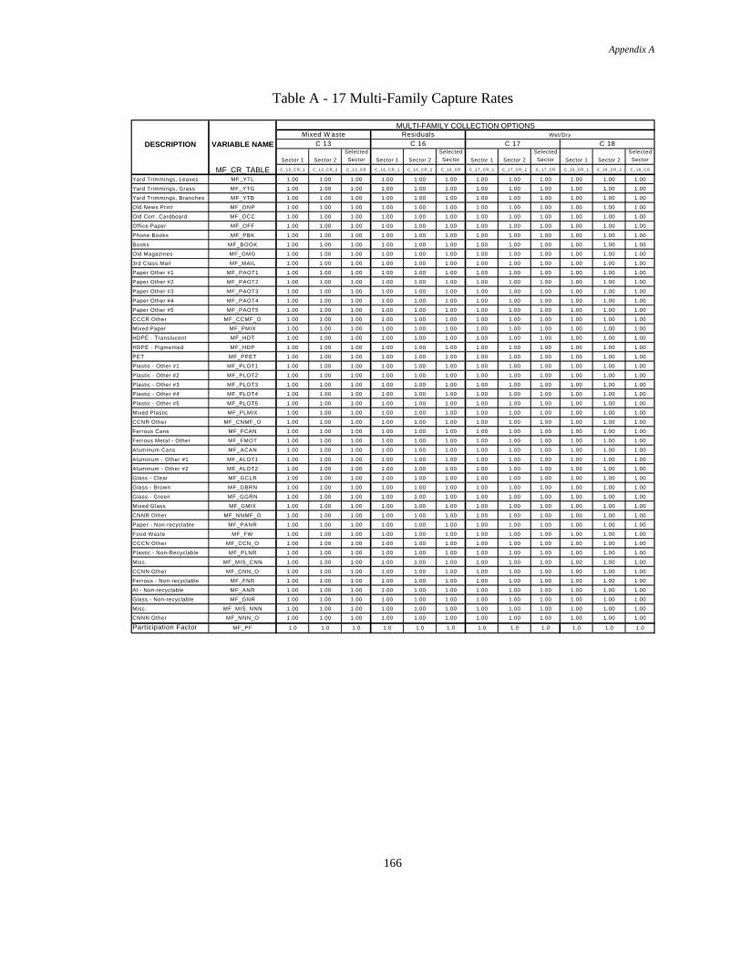
Appendix A
166
Table A - 17 Multi-Family Capture Rates
Mixed W aste Residuals Wet/Dry
DESCRIPTION VARIABLE NAME C 13 C 16 C 17 C 18
Sector 1 Sector 2
Selected Sector Sector 1 Sector 2
Selected Sector Sector 1 Sector 2
Selected Sector Sector 1 Sector 2
Selected Sector
MF_CR_TABLE C_13_CR_1 C_13_CR_2 C_13_CR C_16_CR_1 C_16_CR_2 C_16_CR C_17_CR_1 C_17_CR_2 C_17_CR C_18_CR_1 C_18_CR_2 C_18_CR
Yard Trimmings, Leaves MF_YTL 1.00 1.00 1.00 1.00 1.00 1.00 1.00 1.00 1.00 1.00 1.00 1.00
Yard Trimmings, Grass MF_YTG 1.00 1.00 1.00 1.00 1.00 1.00 1.00 1.00 1.00 1.00 1.00 1.00
Yard Trimmings, Branches MF_YTB 1.00 1.00 1.00 1.00 1.00 1.00 1.00 1.00 1.00 1.00 1.00 1.00
Old News Print MF_ONP 1.00 1.00 1.00 1.00 1.00 1.00 1.00 1.00 1.00 1.00 1.00 1.00
Old Corr. Cardboard MF_OCC 1.00 1.00 1.00 1.00 1.00 1.00 1.00 1.00 1.00 1.00 1.00 1.00
Office Paper MF_OFF 1.00 1.00 1.00 1.00 1.00 1.00 1.00 1.00 1.00 1.00 1.00 1.00
Phone Books MF_PBK 1.00 1.00 1.00 1.00 1.00 1.00 1.00 1.00 1.00 1.00 1.00 1.00
Books MF_BOOK 1.00 1.00 1.00 1.00 1.00 1.00 1.00 1.00 1.00 1.00 1.00 1.00
Old Magazines MF_OMG 1.00 1.00 1.00 1.00 1.00 1.00 1.00 1.00 1.00 1.00 1.00 1.00
3rd Class Mail MF_MAIL 1.00 1.00 1.00 1.00 1.00 1.00 1.00 1.00 1.00 1.00 1.00 1.00
Paper Other #1 MF_PAOT1 1.00 1.00 1.00 1.00 1.00 1.00 1.00 1.00 1.00 1.00 1.00 1.00
Paper Other #2 MF_PAOT2 1.00 1.00 1.00 1.00 1.00 1.00 1.00 1.00 1.00 1.00 1.00 1.00
Paper Other #3 MF_PAOT3 1.00 1.00 1.00 1.00 1.00 1.00 1.00 1.00 1.00 1.00 1.00 1.00
Paper Other #4 MF_PAOT4 1.00 1.00 1.00 1.00 1.00 1.00 1.00 1.00 1.00 1.00 1.00 1.00
Paper Other #5 MF_PAOT5 1.00 1.00 1.00 1.00 1.00 1.00 1.00 1.00 1.00 1.00 1.00 1.00
CCCR Other MF_CCMF_O 1.00 1.00 1.00 1.00 1.00 1.00 1.00 1.00 1.00 1.00 1.00 1.00
Mixed Paper MF_PMIX 1.00 1.00 1.00 1.00 1.00 1.00 1.00 1.00 1.00 1.00 1.00 1.00
HDPE - Translucent MF_HDT 1.00 1.00 1.00 1.00 1.00 1.00 1.00 1.00 1.00 1.00 1.00 1.00
HDPE - Pigmented MF_HDP 1.00 1.00 1.00 1.00 1.00 1.00 1.00 1.00 1.00 1.00 1.00 1.00
PET MF_PPET 1.00 1.00 1.00 1.00 1.00 1.00 1.00 1.00 1.00 1.00 1.00 1.00
Plastic - Other #1 MF_PLOT1 1.00 1.00 1.00 1.00 1.00 1.00 1.00 1.00 1.00 1.00 1.00 1.00
Plastic - Other #2 MF_PLOT2 1.00 1.00 1.00 1.00 1.00 1.00 1.00 1.00 1.00 1.00 1.00 1.00
Plastic - Other #3 MF_PLOT3 1.00 1.00 1.00 1.00 1.00 1.00 1.00 1.00 1.00 1.00 1.00 1.00
Plastic - Other #4 MF_PLOT4 1.00 1.00 1.00 1.00 1.00 1.00 1.00 1.00 1.00 1.00 1.00 1.00
Plastic - Other #5 MF_PLOT5 1.00 1.00 1.00 1.00 1.00 1.00 1.00 1.00 1.00 1.00 1.00 1.00
Mixed Plastic MF_PLMIX 1.00 1.00 1.00 1.00 1.00 1.00 1.00 1.00 1.00 1.00 1.00 1.00
CCNR Other MF_CNMF_O 1.00 1.00 1.00 1.00 1.00 1.00 1.00 1.00 1.00 1.00 1.00 1.00
Ferrous Cans MF_FCAN 1.00 1.00 1.00 1.00 1.00 1.00 1.00 1.00 1.00 1.00 1.00 1.00
Ferrous Metal - Other MF_FMOT 1.00 1.00 1.00 1.00 1.00 1.00 1.00 1.00 1.00 1.00 1.00 1.00
Aluminum Cans MF_ACAN 1.00 1.00 1.00 1.00 1.00 1.00 1.00 1.00 1.00 1.00 1.00 1.00
Aluminum - Other #1 MF_ALOT1 1.00 1.00 1.00 1.00 1.00 1.00 1.00 1.00 1.00 1.00 1.00 1.00
Aluminum - Other #2 MF_ALOT2 1.00 1.00 1.00 1.00 1.00 1.00 1.00 1.00 1.00 1.00 1.00 1.00
Glass - Clear MF_GCLR 1.00 1.00 1.00 1.00 1.00 1.00 1.00 1.00 1.00 1.00 1.00 1.00
Glass - Brown MF_GBRN 1.00 1.00 1.00 1.00 1.00 1.00 1.00 1.00 1.00 1.00 1.00 1.00
Glass - Green MF_GGRN 1.00 1.00 1.00 1.00 1.00 1.00 1.00 1.00 1.00 1.00 1.00 1.00
Mixed Glass MF_GMIX 1.00 1.00 1.00 1.00 1.00 1.00 1.00 1.00 1.00 1.00 1.00 1.00
CNNR Other MF_NNMF_O 1.00 1.00 1.00 1.00 1.00 1.00 1.00 1.00 1.00 1.00 1.00 1.00
Paper - Non-recyclable MF_PANR 1.00 1.00 1.00 1.00 1.00 1.00 1.00 1.00 1.00 1.00 1.00 1.00
Food Waste MF_FW 1.00 1.00 1.00 1.00 1.00 1.00 1.00 1.00 1.00 1.00 1.00 1.00
CCCN Other MF_CCN_O 1.00 1.00 1.00 1.00 1.00 1.00 1.00 1.00 1.00 1.00 1.00 1.00
Plastic - Non-Recyclable MF_PLNR 1.00 1.00 1.00 1.00 1.00 1.00 1.00 1.00 1.00 1.00 1.00 1.00
Misc. MF_MIS_CNN 1.00 1.00 1.00 1.00 1.00 1.00 1.00 1.00 1.00 1.00 1.00 1.00
CCNN Other MF_CNN_O 1.00 1.00 1.00 1.00 1.00 1.00 1.00 1.00 1.00 1.00 1.00 1.00
Ferrous - Non-recyclable MF_FNR 1.00 1.00 1.00 1.00 1.00 1.00 1.00 1.00 1.00 1.00 1.00 1.00
Al - Non-recyclable MF_ANR 1.00 1.00 1.00 1.00 1.00 1.00 1.00 1.00 1.00 1.00 1.00 1.00
Glass - Non-recyclable MF_GNR 1.00 1.00 1.00 1.00 1.00 1.00 1.00 1.00 1.00 1.00 1.00 1.00
Misc. MF_MIS_NNN 1.00 1.00 1.00 1.00 1.00 1.00 1.00 1.00 1.00 1.00 1.00 1.00
CNNN Other MF_NNN_O 1.00 1.00 1.00 1.00 1.00 1.00 1.00 1.00 1.00 1.00 1.00 1.00
Participation Factor MF_PF 1.0 1.0 1.0 1.0 1.0 1.0 1.0 1.0 1.0 1.0 1.0 1.0
MULTI-FAMILY COLLECTION OPTIONS
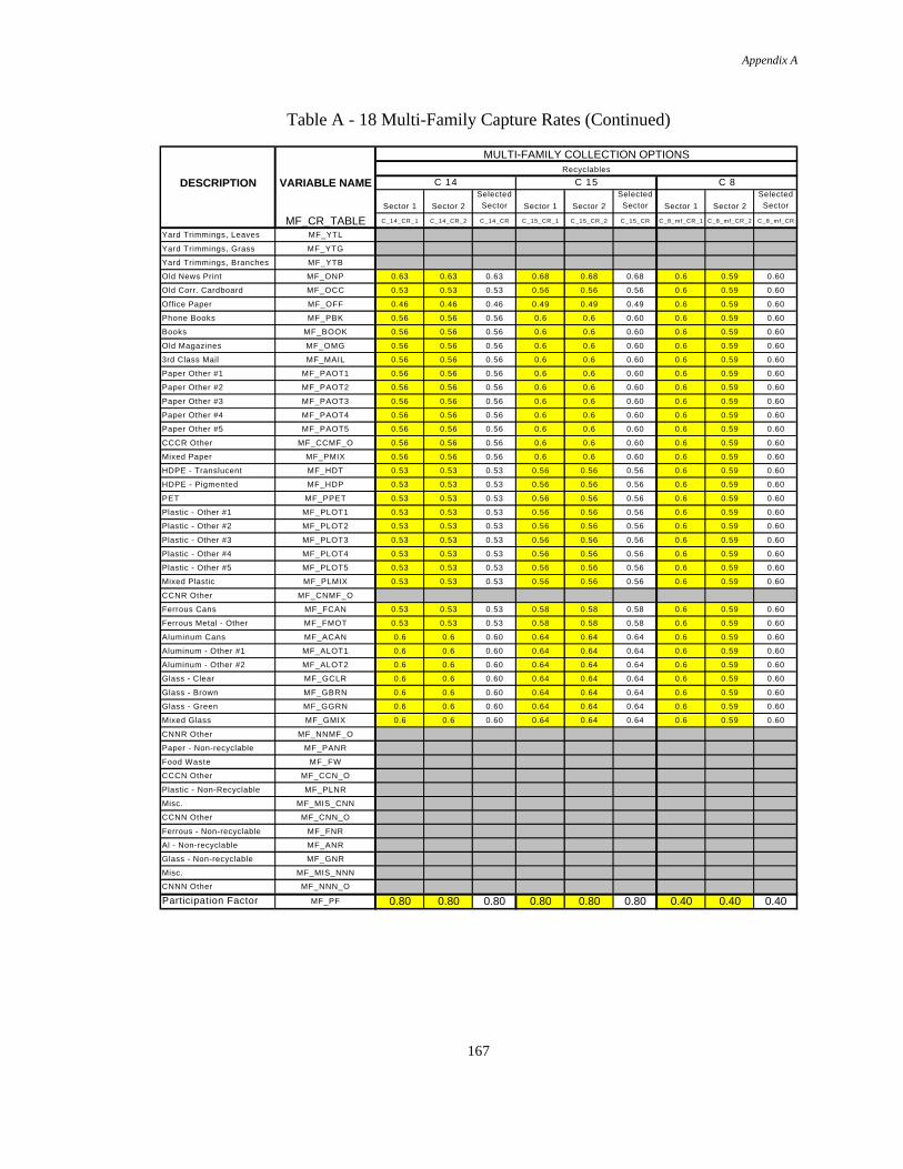
Appendix A
167
Table A - 18 Multi-Family Capture Rates (Continued)
DESCRIPTION VARIABLE NAME C 14 C 15 C 8
Sector 1 Sector 2
Selected Sector Sector 1 Sector 2
Selected Sector Sector 1 Sector 2
Selected Sector
MF_CR_TABLE C_14_CR_1 C_14_CR_2 C_14_CR C_15_CR_1 C_15_CR_2 C_15_CR C_8_mf_CR_1 C_8_mf_CR_2 C_8_mf_CR
Yard Trimmings, Leaves MF_YTL
Yard Trimmings, Grass MF_YTG
Yard Trimmings, Branches MF_YTB
Old News Print MF_ONP 0.63 0.63 0.63 0.68 0.68 0.68 0.6 0.59 0.60
Old Corr. Cardboard MF_OCC 0.53 0.53 0.53 0.56 0.56 0.56 0.6 0.59 0.60
Office Paper MF_OFF 0.46 0.46 0.46 0.49 0.49 0.49 0.6 0.59 0.60
Phone Books MF_PBK 0.56 0.56 0.56 0.6 0.6 0.60 0.6 0.59 0.60
Books MF_BOOK 0.56 0.56 0.56 0.6 0.6 0.60 0.6 0.59 0.60
Old Magazines MF_OMG 0.56 0.56 0.56 0.6 0.6 0.60 0.6 0.59 0.60
3rd Class Mail MF_MAIL 0.56 0.56 0.56 0.6 0.6 0.60 0.6 0.59 0.60
Paper Other #1 MF_PAOT1 0.56 0.56 0.56 0.6 0.6 0.60 0.6 0.59 0.60
Paper Other #2 MF_PAOT2 0.56 0.56 0.56 0.6 0.6 0.60 0.6 0.59 0.60
Paper Other #3 MF_PAOT3 0.56 0.56 0.56 0.6 0.6 0.60 0.6 0.59 0.60
Paper Other #4 MF_PAOT4 0.56 0.56 0.56 0.6 0.6 0.60 0.6 0.59 0.60
Paper Other #5 MF_PAOT5 0.56 0.56 0.56 0.6 0.6 0.60 0.6 0.59 0.60
CCCR Other MF_CCMF_O 0.56 0.56 0.56 0.6 0.6 0.60 0.6 0.59 0.60
Mixed Paper MF_PMIX 0.56 0.56 0.56 0.6 0.6 0.60 0.6 0.59 0.60
HDPE - Translucent MF_HDT 0.53 0.53 0.53 0.56 0.56 0.56 0.6 0.59 0.60
HDPE - Pigmented MF_HDP 0.53 0.53 0.53 0.56 0.56 0.56 0.6 0.59 0.60
PET MF_PPET 0.53 0.53 0.53 0.56 0.56 0.56 0.6 0.59 0.60
Plastic - Other #1 MF_PLOT1 0.53 0.53 0.53 0.56 0.56 0.56 0.6 0.59 0.60
Plastic - Other #2 MF_PLOT2 0.53 0.53 0.53 0.56 0.56 0.56 0.6 0.59 0.60
Plastic - Other #3 MF_PLOT3 0.53 0.53 0.53 0.56 0.56 0.56 0.6 0.59 0.60
Plastic - Other #4 MF_PLOT4 0.53 0.53 0.53 0.56 0.56 0.56 0.6 0.59 0.60
Plastic - Other #5 MF_PLOT5 0.53 0.53 0.53 0.56 0.56 0.56 0.6 0.59 0.60
Mixed Plastic MF_PLMIX 0.53 0.53 0.53 0.56 0.56 0.56 0.6 0.59 0.60
CCNR Other MF_CNMF_O
Ferrous Cans MF_FCAN 0.53 0.53 0.53 0.58 0.58 0.58 0.6 0.59 0.60
Ferrous Metal - Other MF_FMOT 0.53 0.53 0.53 0.58 0.58 0.58 0.6 0.59 0.60
Aluminum Cans MF_ACAN 0.6 0.6 0.60 0.64 0.64 0.64 0.6 0.59 0.60
Aluminum - Other #1 MF_ALOT1 0.6 0.6 0.60 0.64 0.64 0.64 0.6 0.59 0.60
Aluminum - Other #2 MF_ALOT2 0.6 0.6 0.60 0.64 0.64 0.64 0.6 0.59 0.60
Glass - Clear MF_GCLR 0.6 0.6 0.60 0.64 0.64 0.64 0.6 0.59 0.60
Glass - Brown MF_GBRN 0.6 0.6 0.60 0.64 0.64 0.64 0.6 0.59 0.60
Glass - Green MF_GGRN 0.6 0.6 0.60 0.64 0.64 0.64 0.6 0.59 0.60
Mixed Glass MF_GMIX 0.6 0.6 0.60 0.64 0.64 0.64 0.6 0.59 0.60
CNNR Other MF_NNMF_O
Paper - Non-recyclable MF_PANR
Food Waste MF_FW
CCCN Other MF_CCN_O
Plastic - Non-Recyclable MF_PLNR
Misc. MF_MIS_CNN
CCNN Other MF_CNN_O
Ferrous - Non-recyclable MF_FNR
Al - Non-recyclable MF_ANR
Glass - Non-recyclable MF_GNR
Misc. MF_MIS_NNN
CNNN Other MF_NNN_O
Participation Factor MF_PF 0.80 0.80 0.80 0.80 0.80 0.80 0.40 0.40 0.40
Recyclables
MULTI-FAMILY COLLECTION OPTIONS

Appendix A
168
Table A - 19 Commercial Capture Rates
COMMERCIAL COLLECTION OPTIONS
RecyclablesMSW/ Residuals
DESCRIPTION VARIABLE NAME C 19 C 20
Sector 1 Sector 2 Sector 3 Sector 4 Sector 5 Sector 6 Sector 7 Sector 8 Sector 9 Sector 10
Selected
Sector
Selected
Sector
C_CR_TABLE C_19_CR_1 C_19_CR_2 C_19_CR_3 C_19_CR_4 C_19_CR_5 C_19_CR_6 C_19_CR_7 C_19_CR_8 C_19_CR_9 C_19_CR_10 C_19_CR C_20_CR
Yard Trimmings, Leaves C_YTL
Yard Trimmings, Grass C_YTG
Yard Trimmings, Branches C_YTB
Old News Print C_ONP 0.63 0.63 0.63 0.63 0.63 0.63 0.63 0.63 0.63 0.63 0.63Old Corr. Cardboard C_OCC 0.53 0.53 0.53 0.53 0.53 0.53 0.53 0.53 0.53 0.53 0.53Office Paper C_OFF 0.46 0.46 0.46 0.46 0.46 0.46 0.46 0.46 0.46 0.46 0.46Phone Books C_PBK 0.60 0.60 0.60 0.60 0.60 0.60 0.60 0.60 0.60 0.60 0.60Books C_BOOK
Old Magazines C_OMG
3rd Class Mail C_MAIL 0.60 0.60 0.60 0.60 0.60 0.60 0.60 0.60 0.60 0.60 0.60Paper Other #1 C_PAOT1 0.60 0.60 0.60 0.60 0.60 0.60 0.60 0.60 0.60 0.60 0.60Paper Other #2 C_PAOT2 0.60 0.60 0.60 0.60 0.60 0.60 0.60 0.60 0.60 0.60 0.60Paper Other #3 C_PAOT3 0.60 0.60 0.60 0.60 0.60 0.60 0.60 0.60 0.60 0.60 0.60Paper Other #4 C_PAOT4
Paper Other #5 C_PAOT5
CCCR Other C_CCR_O 0.60 0.60 0.60 0.60 0.60 0.60 0.60 0.60 0.60 0.60 0.60Mixed Paper C_PMIX 0.60 0.60 0.60 0.60 0.60 0.60 0.60 0.60 0.60 0.60 0.60HDPE - Translucent C_HDT
HDPE - Pigmented C_HDP
PET C_PPET 0.53 0.53 0.53 0.53 0.53 0.53 0.53 0.53 0.53 0.53 0.53Plastic - Other #1 C_PLOT1
Plastic - Other #2 C_PLOT2
Plastic - Other #3 C_PLOT3
Plastic - Other #4 C_PLOT4
Plastic - Other #5 C_PLOT5
Mixed Plastic C_PLMIX 0.53 0.53 0.53 0.53 0.53 0.53 0.53 0.53 0.53 0.53 0.53CCNR Other C_CNR_O 0.53 0.53 0.53 0.53 0.53 0.53 0.53 0.53 0.53 0.53 0.53Ferrous Cans C_FCAN 0.53 0.53 0.53 0.53 0.53 0.53 0.53 0.53 0.53 0.53 0.53Ferrous Metal - Other C_FMOT 0.50 0.50 0.50 0.50 0.50 0.50 0.50 0.50 0.50 0.50 0.50Aluminum Cans C_ACAN 0.60 0.60 0.60 0.60 0.60 0.60 0.60 0.60 0.60 0.60 0.60Aluminum - Other #1 C_ALOT1
Aluminum - Other #2 C_ALOT2
Glass - Clear C_GCLR 0.60 0.60 0.60 0.60 0.60 0.60 0.60 0.60 0.60 0.60 0.60Glass - Brown C_GBRN 0.60 0.60 0.60 0.60 0.60 0.60 0.60 0.60 0.60 0.60 0.60Glass - Green C_GGRN 0.60 0.60 0.60 0.60 0.60 0.60 0.60 0.60 0.60 0.60 0.60Mixed Glass C_GMIX 0.60 0.60 0.60 0.60 0.60 0.60 0.60 0.60 0.60 0.60 0.60CNNR Other C_NNR_O 0.60 0.60 0.60 0.60 0.60 0.60 0.60 0.60 0.60 0.60 0.60Paper - Non-recyclable C_PANR
Food Waste C_FW
CCCN Other C_CCN_O
Plastic - Non-Recyclable C_PLNR
Misc. C_MIS_CNN
CCNN Other C_CNN_O
Ferrous - Non-recyclable C_FNR
Al - Non-recyclable C_ANR
Glass - Non-recyclable C_GNR
Misc. C_MIS_NNN
CNNN Other C_NNN_O
Participation Factor C_PF 0.50 0.50 0.50 0.50 0.50 0.50 0.50 0.50 0.50 0.50 0.50 1.0

Appendix A
169
Table A - 20 Residential Wet/Dry Separation Factors
W et/Dry/Recyclables W et/Dry
DESCRIPTION Separation Factors Separation Factors
Collection Options C11 & C17 Collection Options C12 & C18
sf_WDR_wet sf_WDR_dry sf_WDR_recyc sf_WD_wet sf_WD_dry
Yard Trimmings, Leaves 1.00 0.00 0.00 1.00 0.00Yard Trimmings, Grass 1.00 0.00 0.00 1.00 0.00Yard Trimmings, Branches 1.00 0.00 0.00 1.00 0.00Old News Print 0.00 0.25 0.75 0.20 0.80Old Corr. Cardboard 0.00 0.25 0.75 0.20 0.80Office Paper 0.00 0.25 0.75 0.20 0.80Phone Books 0.00 0.25 0.75 0.20 0.80Books 0.00 0.25 0.75 0.20 0.80Old Magazines 0.00 0.25 0.75 0.20 0.803rd Class Mail 0.00 0.25 0.75 0.20 0.80Paper Other #1 0.00 0.25 0.75 0.20 0.80Paper Other #2 0.00 0.25 0.75 0.20 0.80Paper Other #3 0.00 0.25 0.75 0.20 0.80Paper Other #4 0.00 0.25 0.75 0.20 0.80Paper Other #5 0.00 0.25 0.75 0.20 0.80CCCR Other
Mixed Paper 0.00 0.25 0.75 0.20 0.80HDPE - Translucent 0.00 0.25 0.75 0.10 0.90HDPE - Pigmented 0.00 0.25 0.75 0.10 0.90PET 0.00 0.25 0.75 0.10 0.90Plastic - Other #1 0.00 0.25 0.75 0.10 0.90Plastic - Other #2 0.00 0.25 0.75 0.10 0.90Plastic - Other #3 0.00 0.25 0.75 0.10 0.90Plastic - Other #4 0.00 0.25 0.75 0.10 0.90Plastic - Other #5 0.00 0.25 0.75 0.10 0.90Mixed Plastic 0.00 0.25 0.75 0.10 0.90CCNR Other
Ferrous Cans 0.00 0.25 0.75 0.10 0.90Ferrous Metal - Other 0.00 0.25 0.75 0.10 0.90Alum inum Cans 0.00 0.25 0.75 0.10 0.90Alum inum - Other #1 0.00 0.25 0.75 0.10 0.90Alum inum - Other #2 0.00 0.25 0.75 0.10 0.90Glass - Clear 0.00 0.25 0.75 0.10 0.90Glass - Brown 0.00 0.25 0.75 0.10 0.90Glass - Green 0.00 0.25 0.75 0.10 0.90Mixed Glass 0.00 0.25 0.75 0.10 0.90CNNR Other
Paper - Non-recyclable 0.00 1.00 0.00 0.25 0.75Food W aste 1.00 0.00 0.00 1.00 0.00CCCN Other
Plastic - Non-Recyclable 0.00 1.00 0.00 0.10 0.90Misc. 0.00 1.00 0.00 0.10 0.90CCNN Other
Ferrous - Non-recyclable 0.00 1.00 0.00 0.10 0.90Al - Non-recyclable 0.00 1.00 0.00 0.10 0.90Glass - Non-recyclable 0.00 1.00 0.00 0.10 0.90Misc. 0.00 1.00 0.00 0.10 0.90CNNN Other

Appendix A
170
Table A - 21 Residential Collection Compaction Factors
Mixed Resi-Residential Collection Options Waste duals Co-Collection Wet/Dry Recyclables
C_1 C_7 C_5 C_6 C_11 C_12 C_2 C_3 C_4 C_0 C_9
Leaves YTL 1.0 1.0 1.0 1.0 1.0
Grass YTG 1.0 1.0 1.0 1.0 1.0
Branches YTB 1.0 1.0 1.0 1.0 1.0
Old News Print ONP 1.0 1.0 1.0 1.0 1.0
Old Corr. Cardboard OCC 1.0 1.0 1.0 1.0 1.0
Office Paper OFF 1.0 1.0 1.0 1.0 1.0
Phone Books PBK 1.0 1.0 1.0 1.0 1.0
Books BOOK 1.0 1.0 1.0 1.0 1.0
Old Magazines OMG 1.0 1.0 1.0 1.0 1.0
3rd Class Mail MAIL 1.0 1.0 1.0 1.0 1.0
Paper Other #1 PAOT1 1.0 1.0 1.0 1.0 1.0
Paper Other #2 PAOT2 1.0 1.0 1.0 1.0 1.0
Paper Other #3 PAOT3 1.0 1.0 1.0 1.0 1.0
Paper Other #4 PAOT4 1.0 1.0 1.0 1.0 1.0
Paper Other #5 PAOT5 1.0 1.0 1.0 1.0 1.0
CCCR Other CCR_O 1.0 1.0 1.0 1.0 1.0
Mixed Paper PMIX 1.0 1.0 1.0 1.0 1.0
HDPE - Translucent HDT 1.0 1.0 1.0 1.0 1.0
HDPE - Pigmented HDP 1.0 1.0 1.0 1.0 1.0
PET PPET 1.0 1.0 1.0 1.0 1.0
Plastic - Other #1 PLOT1 1.0 1.0 1.0 1.0 1.0
Plastic - Other #2 PLOT2 1.0 1.0 1.0 1.0 1.0
Plastic - Other #3 PLOT3 1.0 1.0 1.0 1.0 1.0
Plastic - Other #4 PLOT4 1.0 1.0 1.0 1.0 1.0
Plastic - Other #5 PLOT5 1.0 1.0 1.0 1.0 1.0
Mixed Plastic PLMIX 1.0 1.0 1.0 1.0 1.0
CCNR Other CNR_O 1.0 1.0 1.0 1.0 1.0
Ferrous Cans FCAN 1.0 1.0 1.0 1.0 1.0
Ferrous Metal - Other FMOT 1.0 1.0 1.0 1.0 1.0
Aluminum Cans ACAN 1.0 1.0 1.0 1.0 1.0
Aluminum - Other #1 ALOT1 1.0 1.0 1.0 1.0 1.0
Aluminum - Other #2 ALOT2 1.0 1.0 1.0 1.0 1.0
Glass - Clear GCLR 1.0 1.0 1.0 1.0 1.0
Glass - Brown GBRN 1.0 1.0 1.0 1.0 1.0
Glass - Green GGRN 1.0 1.0 1.0 1.0 1.0
Mixed Glass GMIX 1.0 1.0 1.0 1.0 1.0
CNNR Other NNR_O 1.0 1.0 1.0 1.0 1.0
Paper - Non-recyclable PANR 1.0 1.0 1.0 1.0 1.0
Food Waste F W 1.0 1.0 1.0 1.0 1.0
CCCN Other CCN_O 1.0 1.0 1.0 1.0 1.0
Plastic - Non-Recyclable PLNR 1.0 1.0 1.0 1.0 1.0
Misc. MIS_CNN 1.0 1.0 1.0 1.0 1.0
CCNN Other CNN_O 1.0 1.0 1.0 1.0 1.0
Ferrous - Non-recyclable FNR 1.0 1.0 1.0 1.0 1.0
Al - Non-recyclable ANR 1.0 1.0 1.0 1.0 1.0
Glass - Non-recyclable GNR 1.0 1.0 1.0 1.0 1.0
Misc. MIS_NNN 1.0 1.0 1.0 1.0 1.0
CNNN Other NNN_O 1.0 1.0 1.0 1.0 1.0
Yard Waste
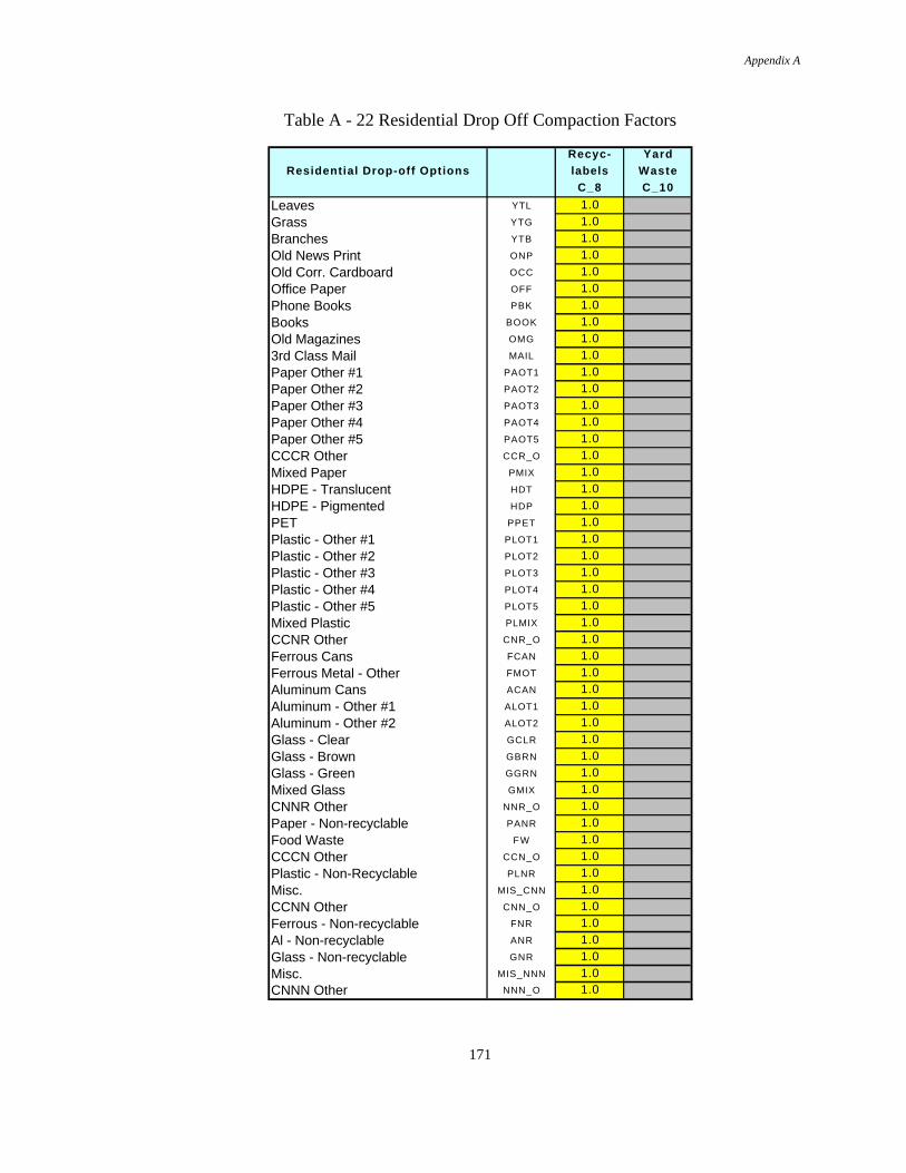
Appendix A
171
Table A - 22 Residential Drop Off Compaction Factors
Recyc- Yard
Residential Drop-off Options labels Waste
C_8 C_10
Leaves YTL 1.0
Grass YTG 1.0
Branches YTB 1.0
Old News Print ONP 1.0
Old Corr. Cardboard OCC 1.0
Office Paper OFF 1.0
Phone Books PBK 1.0
Books BOOK 1.0
Old Magazines OMG 1.0
3rd Class Mail MAIL 1.0
Paper Other #1 PAOT1 1.0
Paper Other #2 PAOT2 1.0
Paper Other #3 PAOT3 1.0
Paper Other #4 PAOT4 1.0
Paper Other #5 PAOT5 1.0
CCCR Other CCR_O 1.0
Mixed Paper PMIX 1.0
HDPE - Translucent HDT 1.0
HDPE - Pigmented HDP 1.0
PET PPET 1.0
Plastic - Other #1 PLOT1 1.0
Plastic - Other #2 PLOT2 1.0
Plastic - Other #3 PLOT3 1.0
Plastic - Other #4 PLOT4 1.0
Plastic - Other #5 PLOT5 1.0
Mixed Plastic PLMIX 1.0
CCNR Other CNR_O 1.0
Ferrous Cans FCAN 1.0
Ferrous Metal - Other FMOT 1.0
Aluminum Cans ACAN 1.0
Aluminum - Other #1 ALOT1 1.0
Aluminum - Other #2 ALOT2 1.0
Glass - Clear GCLR 1.0
Glass - Brown GBRN 1.0
Glass - Green GGRN 1.0
Mixed Glass GMIX 1.0
CNNR Other NNR_O 1.0
Paper - Non-recyclable PANR 1.0
Food Waste FW 1.0
CCCN Other CCN_O 1.0
Plastic - Non-Recyclable PLNR 1.0
Misc. MIS_CNN 1.0
CCNN Other CNN_O 1.0
Ferrous - Non-recyclable FNR 1.0
Al - Non-recyclable ANR 1.0
Glass - Non-recyclable GNR 1.0
Misc. MIS_NNN 1.0
CNNN Other NNN_O 1.0
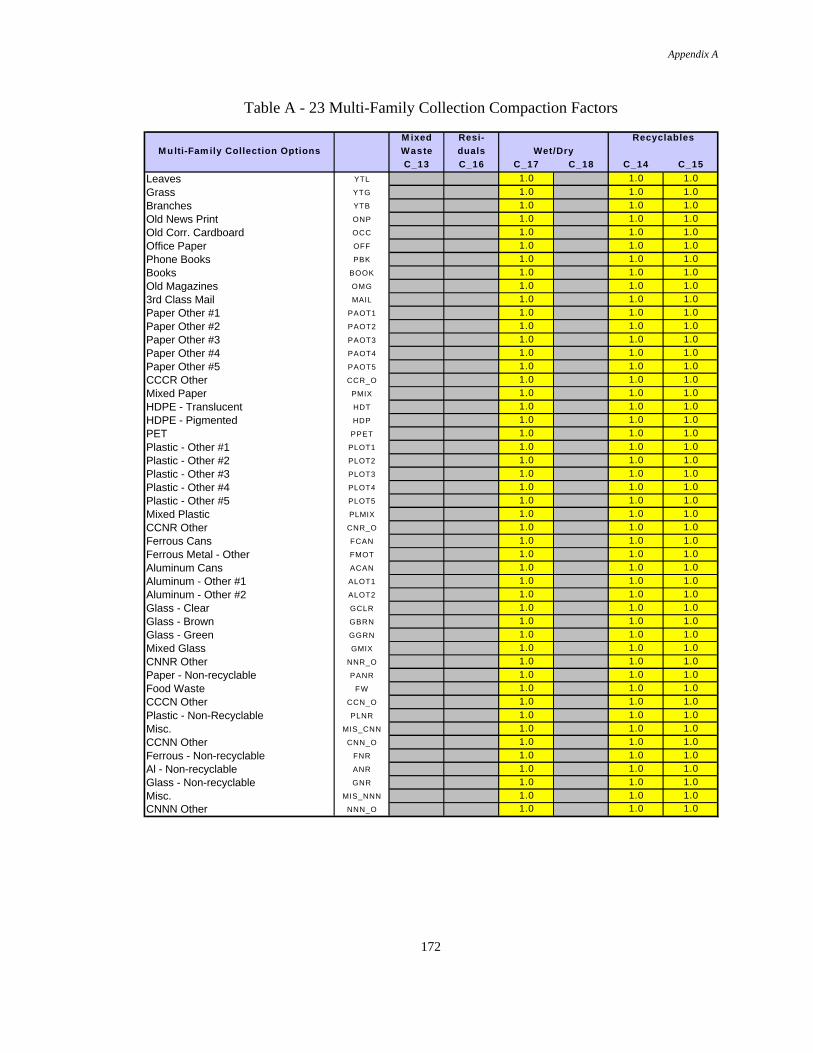
Appendix A
172
Table A - 23 Multi-Family Collection Compaction Factors
M ixed Resi- Recyclables
M u lti-Fam ily Collection Options Waste duals Wet/Dry
C_13 C_16 C_17 C_18 C_14 C_15
Leaves YTL 1.0 1.0 1.0
Grass YTG 1.0 1.0 1.0
Branches YTB 1.0 1.0 1.0
Old News Print ONP 1.0 1.0 1.0
Old Corr. Cardboard OCC 1.0 1.0 1.0
Office Paper OFF 1.0 1.0 1.0
Phone Books PBK 1.0 1.0 1.0
Books BOOK 1.0 1.0 1.0
Old Magazines OMG 1.0 1.0 1.0
3rd Class Mail MAIL 1.0 1.0 1.0
Paper Other #1 PAOT1 1.0 1.0 1.0
Paper Other #2 PAOT2 1.0 1.0 1.0
Paper Other #3 PAOT3 1.0 1.0 1.0
Paper Other #4 PAOT4 1.0 1.0 1.0
Paper Other #5 PAOT5 1.0 1.0 1.0
CCCR Other CCR_O 1.0 1.0 1.0
Mixed Paper PMIX 1.0 1.0 1.0
HDPE - Translucent HDT 1.0 1.0 1.0
HDPE - Pigmented HDP 1.0 1.0 1.0
PET PPET 1.0 1.0 1.0
Plastic - Other #1 PLOT1 1.0 1.0 1.0
Plastic - Other #2 PLOT2 1.0 1.0 1.0
Plastic - Other #3 PLOT3 1.0 1.0 1.0
Plastic - Other #4 PLOT4 1.0 1.0 1.0
Plastic - Other #5 PLOT5 1.0 1.0 1.0
Mixed Plastic PLMIX 1.0 1.0 1.0
CCNR Other CNR_O 1.0 1.0 1.0
Ferrous Cans FCAN 1.0 1.0 1.0
Ferrous Metal - Other FMOT 1.0 1.0 1.0
Aluminum Cans ACAN 1.0 1.0 1.0
Aluminum - Other #1 ALOT1 1.0 1.0 1.0
Aluminum - Other #2 ALOT2 1.0 1.0 1.0
Glass - Clear GCLR 1.0 1.0 1.0
Glass - Brown GBRN 1.0 1.0 1.0
Glass - Green GGRN 1.0 1.0 1.0
Mixed Glass GMIX 1.0 1.0 1.0
CNNR Other NNR_O 1.0 1.0 1.0
Paper - Non-recyclable PANR 1.0 1.0 1.0
Food Waste FW 1.0 1.0 1.0
CCCN Other CCN_O 1.0 1.0 1.0
Plastic - Non-Recyclable PLNR 1.0 1.0 1.0
Misc. MIS_CNN 1.0 1.0 1.0
CCNN Other CNN_O 1.0 1.0 1.0
Ferrous - Non-recyclable FNR 1.0 1.0 1.0
Al - Non-recyclable ANR 1.0 1.0 1.0
Glass - Non-recyclable GNR 1.0 1.0 1.0
Misc. MIS_NNN 1.0 1.0 1.0CNNN Other NNN_O 1.0 1.0 1.0

Appendix A
173
Table A - 24 Commercial Collection Compaction Factors
Recyc- M S W /
Commercial Collection Options labels Residuals
C_19 C_20
Leaves YTL 1.0
Grass YTG 1.0
Branches YTB 1.0
Old News Print ONP 1.0
Old Corr. Cardboard OCC 1.0
Office Paper OFF 1.0
Phone Books PBK 1.0
Books BOOK 1.0
Old Magazines OMG 1.0
3rd Class Mail MAIL 1.0
Paper Other #1 PAOT1 1.0
Paper Other #2 PAOT2 1.0
Paper Other #3 PAOT3 1.0
Paper Other #4 PAOT4 1.0
Paper Other #5 PAOT5 1.0
CCCR Other CCR_O 1.0
Mixed Paper PMIX 1.0
HDPE - Translucent HDT 1.0
HDPE - Pigmented HDP 1.0
PET PPET 1.0
Plastic - Other #1 PLOT1 1.0
Plastic - Other #2 PLOT2 1.0
Plastic - Other #3 PLOT3 1.0
Plastic - Other #4 PLOT4 1.0
Plastic - Other #5 PLOT5 1.0
Mixed Plastic PLMIX 1.0
CCNR Other CNR_O 1.0
Ferrous Cans FCAN 1.0
Ferrous Metal - Other FMOT 1.0
Aluminum Cans ACAN 1.0
Aluminum - Other #1 ALOT1 1.0
Aluminum - Other #2 ALOT2 1.0
Glass - Clear GCLR 1.0
Glass - Brown GBRN 1.0
Glass - Green GGRN 1.0
Mixed Glass GMIX 1.0
CNNR Other NNR_O 1.0
Paper - Non-recyclable PANR 1.0
Food Waste FW 1.0
CCCN Other CCN_O 1.0
Plastic - Non-Recyclable PLNR 1.0
Misc. MIS_CNN 1.0
CCNN Other CNN_O 1.0
Ferrous - Non-recyclable FNR 1.0
Al - Non-recyclable ANR 1.0
Glass - Non-recyclable GNR 1.0
Misc. MIS_NNN 1.0
CNNN Other NNN_O 1.0

Appendix A
174
Table A - 25 Process Model Interest Rates
DESCRIPTION VARIABLE NAME VALUE UNITSMRF interest Rate MRF_I 5% %Transfer Station interest rate TR_I 10% %Landfill Interest Rate LF_I 5% %Collection Interest Rate COL_I 5% %Combustor Interest Rate CF_I 5% %MSW Compost Interest Rate MSW_C_I 5% %RDF Interest Rate RDF_I 5% %Anerobic Digestion Interest Rate DIG_I 5% %Yard Waste Compost Interest Rate YW_I 5% %

Appendix A
175
Table A - 26 Generation Rate Data
DESCRIPTION VARIABLE NAME VALUE UNITSCommunity Name comm_name W ake County N/AResidential Population 1 res_pop_1 200,000 peopleResidents per house 1 res_per_dwel_1 2.63 people/houseGeneration rate 1 res_gen_1 2.88 lb/person-day
Residential Population 2 res_pop_2 2,000 peopleResidents per house 2 res_per_dwel_2 2.63 people/houseGeneration rate 2 res_gen_2 2.88 lb/person-dayCurrently Selected Residential Population res_pop 200,000 peopleCurrently Selected Residents per House ph 2.63 people/houseCurrently Selected Residential Generation Rate gr 2.88 lb/person-dayCurrently Selected Houses in Sector h_res 76,046 housesCurrently Selected Residential Waste Generation Rate g_res 53.02 lb/house-week
Multi-Fam ily Population 1 m f_pop_1 20,000 peopleGeneration rate 1 m f_gen_1 2.88 lb/person-dayNumber of Multi-family collection locations 1 mf_loc_1 100 locationsMulti-Fam ily Population 2 m f_pop_2 1,000 peopleGeneration rate 2 m f_gen_2 2.88 lb/person-dayNumber of Multi-family collection locations 2 mf_loc_2 10 locations
Currently Selected MF Population mf_pop 20,000 peopleCurrently Selected MF Generation Rate mf_gen 2.88 lb/person-dayCurrently Selected Number of Multi-family collection locations h_mf 100 locationsMulti-family Waste Generation Rate (lb/location-week) g_mf 4,032.00 lb/location-weekNumber of Commercial Collection locations 1 com_loc_1 100 locationsNumber of Commercial Collection locations 2 com_loc_2 100 locationsNumber of Commercial Collection locations 3 com_loc_3 100 locationsNumber of Commercial Collection locations 4 com_loC_9 100 locationsNumber of Commercial Collection locations 5 com_loc_5 100 locationsNumber of Commercial Collection locations 6 com_loc_6 100 locationsNumber of Commercial Collection locations 7 com_loc_7 100 locationsNumber of Commercial Collection locations 8 com_loc_8 100 locationsNumber of Commercial Collection locations 9 com_loc_9 100 locationsNumber of Commercial Collection locations 10 com_loc_10 100 locationsCommercial Waste Generation Rate 1 com_gen_1 2,300 lb/location-weekCommercial Waste Generation Rate 2 com_gen_2 2,300 lb/location-weekCommercial Waste Generation Rate 3 com_gen_3 2,300 lb/location-weekCommercial Waste Generation Rate 4 com_gen_4 2,300 lb/location-weekCommercial Waste Generation Rate 5 com_gen_5 2,300 lb/location-weekCommercial Waste Generation Rate 6 com_gen_6 2,300 lb/location-weekCommercial Waste Generation Rate 7 com_gen_7 2,300 lb/location-weekCommercial Waste Generation Rate 8 com_gen_8 2,300 lb/location-weekCommercial Waste Generation Rate 9 com_gen_9 2,300 lb/location-weekCommercial Waste Generation Rate 10 com_gen_10 2,300 lb/location-weekCurrently Selected Commercial Collection locations h_com 100 locationsCurrently Selected Commercial Waste Generation Rate g_com 2,300 lb/location-week

Appendix A
176
Table A - 27 Residential Composition
Density in Density in Default Sector #1 Sector #1 Sector #1 Sector #2 Sector #2 Sector #2 Currently
DESCRIPTION VARIABLE NAME Refuse Recycling Residential User Non-Override Model User Non-Override Model Selected
Collection Collection Composition Override Fraction Value Override Fraction Value Residential
Vehicle Vehicle (wt. fraction) (wt. fraction) (wt. fraction) (wt. fraction) (wt. fraction) (wt. fraction) (wt. fraction) Values
(lb/yd3) (lb/yd3)
MSW_COMP_TABLE D_cv D_rcv RES_WT_FRAC_1 RES_WT_FRAC_2 RES_WT_FRAC
Yard Trimmings, Leaves YTL 550 350 0.056 0.142 0.000 0.142 0.000 0.056 0.056 0.142
Yard Trimmings, Grass YTG 550 350 0.093 0.043 0.000 0.043 0.000 0.093 0.093 0.043
Yard Trimmings, Branches YTB 550 350 0.037 0.041 0.000 0.041 0.000 0.037 0.037 0.041
Old News Print ONP 550 500 0.067 0.075 0.000 0.075 0.000 0.067 0.067 0.075
Old Corr. Cardboard OCC 550 150 0.021 0.018 0.000 0.018 0.000 0.021 0.021 0.018
Office Paper OFF 550 500 0.013 0.012 0.000 0.012 0.000 0.013 0.013 0.012
Phone Books PBK 550 500 0.002 0.003 0.000 0.000 0.000 0.002 0.000 0.000
Books BOOK 550 500 0.009 0.005 0.000 0.005 0.000 0.009 0.009 0.005
Old Magazines OMG 550 500 0.017 0.011 0.000 0.011 0.000 0.017 0.017 0.011
3rd Class Mail MAIL 550 500 0.022 0.018 0.000 0.000 0.000 0.022 0.000 0.000
Paper Other #1 PAOT1 550 500 0.000 0.024 0.000 0.024 0.000 0.000 0.000 0.024
Paper Other #2 PAOT2 550 500 0.000 0.020 0.000 0.020 0.000 0.000 0.000 0.020
Paper Other #3 PAOT3 550 500 0.000 0.014 0.000 0.014 0.000 0.000 0.000 0.014
Paper Other #4 PAOT4 550 500 0.000 0.001 0.000 0.001 0.000 0.000 0.000 0.001
Paper Other #5 PAOT5 550 500 0.000 0.001 0.000 0.001 0.000 0.000 0.000 0.001
CCCR Other CCR_O 550 500
Mixed Paper PMIX 550 500 0.000 0.021 0.024 0.021
HDPE - Translucent HDT 550 24 0.004 0.014 0.000 0.014 0.000 0.004 0.004 0.014
HDPE - Pigmented HDP 550 24 0.005 0.006 0.000 0.006 0.000 0.005 0.005 0.006
PET PPET 550 40 0.004 0.005 0.000 0.005 0.000 0.004 0.004 0.005
Plastic - Other #1 PLOT1 550 50 0.000 0.043 0.000 0.000 0.000 0.000 0.000 0.000
Plastic - Other #2 PLOT2 550 50 0.000 0.032 0.000 0.000 0.000 0.000 0.000 0.000
Plastic - Other #3 PLOT3 550 50 0.000 0.021 0.000 0.000 0.000 0.000 0.000 0.000
Plastic - Other #4 PLOT4 550 50 0.000 0.003 0.000 0.003 0.000 0.000 0.000 0.003
Plastic - Other #5 PLOT5 550 50 0.000 0.001 0.000 0.001 0.000 0.000 0.000 0.001
Mixed Plastic PLMIX 550 50 0.000 0.096 0.000 0.096
CCNR Other CNR_O 550 50
Ferrous Cans FCAN 550 150 0.015 0.016 0.000 0.016 0.000 0.015 0.015 0.016
Ferrous Metal - Other FMOT 550 750 0.000 0.070 0.000 0.070 0.000 0.000 0.000 0.070
Aluminum Cans ACAN 550 75 0.009 0.009 0.000 0.009 0.000 0.009 0.009 0.009
Aluminum - Other #1 ALOT1 550 400 0.000 0.002 0.000 0.002 0.000 0.000 0.000 0.002
Aluminum - Other #2 ALOT2 550 400 0.000 0.006 0.000 0.006 0.000 0.000 0.000 0.006
Glass - Clear GCLR 550 400 0.039 0.029 0.000 0.029 0.000 0.039 0.039 0.029
Glass - Brown GBRN 550 400 0.016 0.030 0.000 0.030 0.000 0.016 0.016 0.030
Glass - Green GGRN 550 400 0.010 0.010 0.000 0.010 0.000 0.010 0.010 0.010
Mixed Glass GMIX 550 400 0.000 0.000 0.000 0.000
CNNR Other NNR_O 550 150
Paper - Non-recyclable PANR 550 500 0.171 0.055 0.000 0.055 0.000 0.171 0.171 0.055
Food Waste FW 550 800 0.049 0.095 0.000 0.095 0.000 0.049 0.049 0.095
CCCN Other CCN_O 550 700
Plastic - Non-Recyclable PLNR 550 50 0.099 0.008 0.000 0.008 0.000 0.099 0.099 0.008
Misc. MIS_CNN 550 110 0.075 0.106 0.000 0.106 0.000 0.075 0.075 0.106
CCNN Other CNN_O 550 110
Ferrous - Non-recyclable FNR 550 750 0.032 0.003 0.000 0.003 0.000 0.032 0.032 0.003
Al - Non-recyclable ANR 550 400 0.005 0.001 0.000 0.001 0.000 0.005 0.005 0.001
Glass - Non-recyclable GNR 550 400 0.007 0.010 0.000 0.010 0.000 0.007 0.007 0.010
Misc. MIS_NNN 550 300 0.123 0.000 0.000 0.000 0.000 0.123 0.123 0.000
CNNN Other NNN_O 550 400
Densities (All Sectors) Residential Composition

Appendix A
177
Table A - 28 Multi-Family Composition
Default Sector #1 Sector #1 Sector #1 Sector #2 Sector #2 Sector #2 Currently
DESCRIPTION VARIABLE NAME Mult. Family User Non-Override Model User Non-Override Model Selected
Composition Override Fraction Value Override Fraction Value Multi-family
(wt. fraction) (wt. fraction) (wt. fraction) (wt. fraction) (wt. fraction) (wt. fraction) (wt. fraction) Values
MSW_COMP_TABLE MF_WT_FRAC_1 MF_WT_FRAC_2 M F _ W T _ F R A C
Yard Trimmings, Leaves YTL 0.056 0.142 0.000 0.142 0.000 0.056 0.056 0.142
Yard Trimmings, Grass YTG 0.093 0.043 0.000 0.043 0.000 0.093 0.093 0.043
Yard Trimmings, Branches YTB 0.037 0.041 0.000 0.041 0.000 0.037 0.037 0.041
Old News Print ONP 0.067 0.075 0.000 0.075 0.000 0.067 0.067 0.075
Old Corr. Cardboard OCC 0.021 0.018 0.000 0.018 0.000 0.021 0.021 0.018
Office Paper OFF 0.013 0.012 0.000 0.012 0.000 0.013 0.013 0.012
Phone Books PBK 0.002 0.003 0.000 0.000 0.000 0.002 0.000 0.000
Books BOOK 0.009 0.005 0.000 0.005 0.000 0.009 0.009 0.005
Old Magazines OMG 0.017 0.011 0.000 0.011 0.000 0.017 0.017 0.011
3rd Class Mail MAIL 0.022 0.018 0.000 0.000 0.000 0.022 0.000 0.000
Paper Other #1 PAOT1 0.000 0.024 0.000 0.024 0.000 0.000 0.000 0.024
Paper Other #2 PAOT2 0.000 0.020 0.000 0.020 0.000 0.000 0.000 0.020
Paper Other #3 PAOT3 0.000 0.014 0.000 0.014 0.000 0.000 0.000 0.014
Paper Other #4 PAOT4 0.000 0.001 0.000 0.001 0.000 0.000 0.000 0.001
Paper Other #5 PAOT5 0.000 0.001 0.000 0.001 0.000 0.000 0.000 0.001
CCCR Other CCR_O
Mixed Paper PMIX 0.000 0.021 0.024 0.021
HDPE - Translucent HDT 0.004 0.014 0.000 0.014 0.000 0.004 0.004 0.014
HDPE - Pigmented HDP 0.005 0.006 0.000 0.006 0.000 0.005 0.005 0.006
PET PPET 0.004 0.005 0.000 0.005 0.000 0.004 0.004 0.005
Plastic - Other #1 PLOT1 0.000 0.043 0.000 0.000 0.000 0.000 0.000 0.000
Plastic - Other #2 PLOT2 0.000 0.032 0.000 0.000 0.000 0.000 0.000 0.000
Plastic - Other #3 PLOT3 0.000 0.021 0.000 0.000 0.000 0.000 0.000 0.000
Plastic - Other #4 PLOT4 0.000 0.003 0.000 0.003 0.000 0.000 0.000 0.003
Plastic - Other #5 PLOT5 0.000 0.001 0.000 0.001 0.000 0.000 0.000 0.001
Mixed Plastic PLMIX 0.000 0.096 0.000 0.096
CCNR Other CNR_O
Ferrous Cans FCAN 0.015 0.016 0.000 0.016 0.000 0.015 0.015 0.016
Ferrous Metal - Other FMOT 0.000 0.070 0.000 0.070 0.000 0.000 0.000 0.070
Aluminum Cans ACAN 0.009 0.009 0.000 0.009 0.000 0.009 0.009 0.009
Aluminum - Other #1 ALOT1 0.000 0.002 0.000 0.002 0.000 0.000 0.000 0.002
Aluminum - Other #2 ALOT2 0.000 0.006 0.000 0.006 0.000 0.000 0.000 0.006
Glass - Clear GCLR 0.039 0.029 0.000 0.029 0.000 0.039 0.039 0.029
Glass - Brown GBRN 0.016 0.030 0.000 0.030 0.000 0.016 0.016 0.030
Glass - Green GGRN 0.010 0.010 0.000 0.010 0.000 0.010 0.010 0.010
Mixed Glass GMIX 0.000 0.000 0.000 0.000
CNNR Other NNR_O
Paper - Non-recyclable PANR 0.171 0.055 0.000 0.055 0.000 0.171 0.171 0.055
Food Waste FW 0.049 0.095 0.000 0.095 0.000 0.049 0.049 0.095
CCCN Other CCN_O
Plastic - Non-Recyclable PLNR 0.099 0.008 0.000 0.008 0.000 0.099 0.099 0.008
Misc. MIS_CNN 0.075 0.106 0.000 0.106 0.000 0.075 0.075 0.106
CCNN Other CNN_O
Ferrous - Non-recyclable FNR 0.032 0.003 0.000 0.003 0.000 0.032 0.032 0.003
Al - Non-recyclable ANR 0.005 0.001 0.000 0.001 0.000 0.005 0.005 0.001
Glass - Non-recyclable GNR 0.007 0.010 0.000 0.010 0.000 0.007 0.007 0.010
Misc. MIS_NNN 0.123 0.000 0.000 0.000 0.000 0.123 0.123 0.000
CNNN Other NNN_O

Appendix A
178
Table A - 29 Commercial Composition
Default Sector #1 Sector #1 Sector #1 Sector #10 Sector #10 Sector #10 Currently
DESCRIPTION VARIABLE NAME Commercial User Non-Override Model . . . . . User Non-Override Model Selected
Composition Override Fraction Value Override Fraction Value Commercial
(wt. fraction) (wt. fraction) (wt. fraction) (wt. fraction) (wt. fraction) (wt. fraction) (wt. fraction) Values
MSW_COMP_TABLE COM_WT_FRAC_1 COM_WT_FRAC_10 COM_WT_FRAC
Yard Trimmings, Leaves YTL . . . . .Yard Trimmings, Grass YTG
Yard Trimmings, Branches YTB
Old News Print ONP 0.022 0.000 0.022 0.022 0.000 0.022 0.022 0.0220
Old Corr. Cardboard OCC 0.360 0.000 0.360 0.360 . . . . . 0.000 0.360 0.360 0.3600
Office Paper OFF 0.072 0.000 0.072 0.072 0.000 0.072 0.072 0.0720
Phone Books PBK 0.003 0.000 0.003 0.000 0.000 0.003 0.000 0.0000
Books BOOK
Old Magazines OMG
3rd Class Mail MAIL 0.023 0.000 0.023 0.000 . . . . . 0.000 0.023 0.000 0.0000
Paper Other #1 PAOT1 0.000 0.000 0.000 0.000 0.000 0.000 0.000 0.0000
Paper Other #2 PAOT2 0.000 0.000 0.000 0.000 0.000 0.000 0.000 0.0000
Paper Other #3 PAOT3 0.000 0.000 0.000 0.000 0.000 0.000 0.000 0.0000
Paper Other #4 PAOT4
Paper Other #5 PAOT5 . . . . .CCCR Other CCR_O 0.019 0.000 0.019 0.019 0.000 0.019 0.019 0.0190
Mixed Paper PMIX 0.026 0.026 0.0260
HDPE - Translucent HDT
HDPE - Pigmented HDP
PET PPET 0.002 0.000 0.002 0.002 . . . . . 0.000 0.002 0.002 0.0020
Plastic - Other #1 PLOT1
Plastic - Other #2 PLOT2
Plastic - Other #3 PLOT3
Plastic - Other #4 PLOT4
Plastic - Other #5 PLOT5 . . . . .Mixed Plastic PLMIX 0.000 0.000 0.0000
CCNR Other CNR_O 0.041 0.000 0.041 0.041 0.000 0.041 0.041 0.0410
Ferrous Cans FCAN 0.007 0.000 0.007 0.007 0.000 0.007 0.007 0.0070
Ferrous Metal - Other FMOT
Aluminum Cans ACAN 0.004 0.000 0.004 0.004 . . . . . 0.000 0.004 0.004 0.0040
Aluminum - Other #1 ALOT1
Aluminum - Other #2 ALOT2
Glass - Clear GCLR 0.019 0.000 0.019 0.019 0.000 0.019 0.019 0.0190
Glass - Brown GBRN 0.008 0.000 0.008 0.008 0.000 0.008 0.008 0.0080
Glass - Green GGRN 0.005 0.000 0.005 0.005 0.000 0.005 0.005 0.0050
Mixed Glass GMIX 0.000 . . . . . 0.000 0.0000
CNNR Other NNR_O 0.024 0.000 0.024 0.024 0.000 0.024 0.024 0.0240
Paper - Non-recyclable PANR
Food Waste FW
CCCN Other CCN_O 0.171 0.000 0.171 0.171 0.000 0.171 0.171 0.1710
Plastic - Non-Recyclable PLNR . . . . .Misc. MIS_CNN
CCNN Other CNN_O 0.113 0.000 0.113 0.113 0.000 0.113 0.113 0.1130
Ferrous - Non-recyclable FNR
Al - Non-recyclable ANR . . . . .Glass - Non-recyclable GNR
Misc. MIS_NNN
CNNN Other NNN_O 0.107 0.000 0.107 0.107 0.000 0.107 0.107 0.1070

Appendix A
179
Table A - 30 Transportation Fuel Pre-Combustion Emissions
DESCRIPTION VARIABLE NAME
DIESEL pre comb. (lbs
emission per 1000 gal.
combusted)
GASOLINE pre comb. (lbs emission per
1000 gal. combusted)
Trans_fuel_pre_comb_table d_pc_em g_pc_em
Atmospheric EmissionsParticulates (PM10) T_F_PC_A_PART_10 0 0Particulates (Total) T_F_PC_A_PART 1.82 1.54Nitrogen Oxides T_F_PC_A_NO 7.19 6.06Hydrocarbons (non CH4) T_F_PC_A_HC 67.49014 57.29012Sulfur Oxides T_F_PC_A_SO 8.8 7.44Carbon Monoxide T_F_PC_A_CO 5.01 4.2CO2 (biomass) T_F_PC_A_CO2_BM 0 0CO2 (non biomass) T_F_PC_A_CO2 3594 3034Ammonia T_F_PC_A_NH3 0.039 0.033Lead T_F_PC_A_PB 1.10E-05 0.0000091Methane T_F_PC_A_CH4 0.05 0.043Hydrochloric acid T_F_PC_A_HCL 0.0012 0.00098
Solid WasteSolid Waste #1 T_F_PC_SW_1 82.4 69.7Solid Waste #2 T_F_PC_SW_2 0 0Solid Waste #3 T_F_PC_SW_3 0 0Solid Waste #4 T_F_PC_SW_4 0 0Solid Waste #5 T_F_PC_SW_5 0 0
Waterborne EmissionsDissolved Solids T_F_PC_W_DS 102 86.9Suspended Solids T_F_PC_W_SS 0.095 0.081BOD T_F_PC_W_BOD 0.1 0.089COD T_F_PC_W_COD 0.49058 0.4205Oil T_F_PC_W_OIL 1.23 1.05Sulfuric Acid T_F_PC_W_H2SO4 0.31 0.26Iron T_F_PC_W_FE 0.081 0.068Ammonia T_F_PC_W_NH3 0.014 0.012Copper T_F_PC_W_Cu 0 0Cadmium T_F_PC_W_Cd 0 0Arsenic T_F_PC_W_As 0 0Mercury T_F_PC_W_Hg 0 0Phosphate T_F_PC_W_P_x 0 0Selenium T_F_PC_W_Se 0 0Chromium T_F_PC_W_CR 3.40E-05 0Lead T_F_PC_W_PB 1.50E-05 1.30E-05Zinc T_F_PC_W_ZN 2.20E-04 1.90E-04

Appendix A
180
Table A - 31 Transportation Fuel Pre-Combustion Energy
DESCRIPTION VARIABLE NAME
pre comb. energy
(btu/gal.)
Gasoline - mobil source gas_pc_enrg 2.19E+04Diesel - mobil source dsl_pc_enrg 2.59E+04
Table A - 32 Transportation Fuel Combustion Energy
DESCRIPTION VARIABLE NAME comb. energy (btu/gal.)
Gasoline - mobil source gas_enrg 1.51E+05Diesel - mobil source dsl_enrg 1.37E+05
Table A - 33 Greenhouse Gas Equivalents
GREENHOUSE GAS variable name
20 Year Global
Warming
Potential
Carbon dioxide (fossil fuel) CO2_f_GWP 1Carbon dioxide (biomass) CO2_bm_GWP 0Methane CH4_GWP 63Nitrous Oxide NO_GWP 270Other hydrocarbons HC_GWP 0

Appendix A
181
Table A - 34 Electric Energy Emissions
TOTALEmissions
(lb/kwh elect.)variable name Regional Grid
100.00%emissions
table r_tot
Atmospheric EmissionsParticulates (PM10) a_pm_10 0.00E+00
Particulates (Total) a_pm 2.60E-03
Nitrogen Oxides a_no 6.46E-03
Hydrocarbons (non CH4) a_hc 1.02E-03
Sulfur Oxides a_so 1.37E-02
Carbon Monoxide a_co 2.14E-03
CO2 (biomass) a_co2_bm 0.00E+00
CO2 (non biomass) a_co2 1.49E+00
Ammonia a_nh4 1.76E-07
Lead a_pb 4.91E-11
Methane a_ch4 9.85E-06
Hydrochloric acid a_hcl 5.31E-09
Solid WasteSolid Waste #1 sw_1 1.91E-01
Solid Waste #2 sw_2 0.00E+00
Solid Waste #3 sw_3 0.00E+00
Solid Waste #4 sw_4 0.00E+00
Solid Waste #5 sw_5 0.00E+00
Waterborne EmissionsDissolved Solids w_ds 4.57E-04
Suspended Solids w_ss 4.12E-07
BOD w_bod 4.51E-07
COD w_cod 2.23E-06
Oil w_oil 6.11E-06
Sulfuric Acid w_h2so4 1.12E-03
Iron w_fe 2.79E-04
Ammonia w_nh4 6.15E-08
Copper w_cu 0.00E+00
Cadmium w_cd 0.00E+00
Arsenic w_as 0.00E+00
Mercury w_hg 0.00E+00
Phosphate w_po4 0.00E+00
Selenium w_se 0.00E+00
Chromium w_cr 7.10E-11
Lead w_pb 6.57E-11
Zinc w_zn 9.82E-10
FUEL RELATED EMISSIONS BY USAGE

Appendix B
182
APPENDIX B
DEFAULT INPUT VALUES(FOR VARIABLES WITH SECTOR VARIABILITY)

Appendix B
183
Solid vertical lines are used in the printout to separate collection options into sets ofoptions that are similar to each other. Lightly shaded cells represent input variableswhich might be expected to have a unique value for the option in which the shaded cellappears. Darkly shaded cells represent input variables that are used in the area of thespreadsheet shown, but which are entered in some other location in the process model.
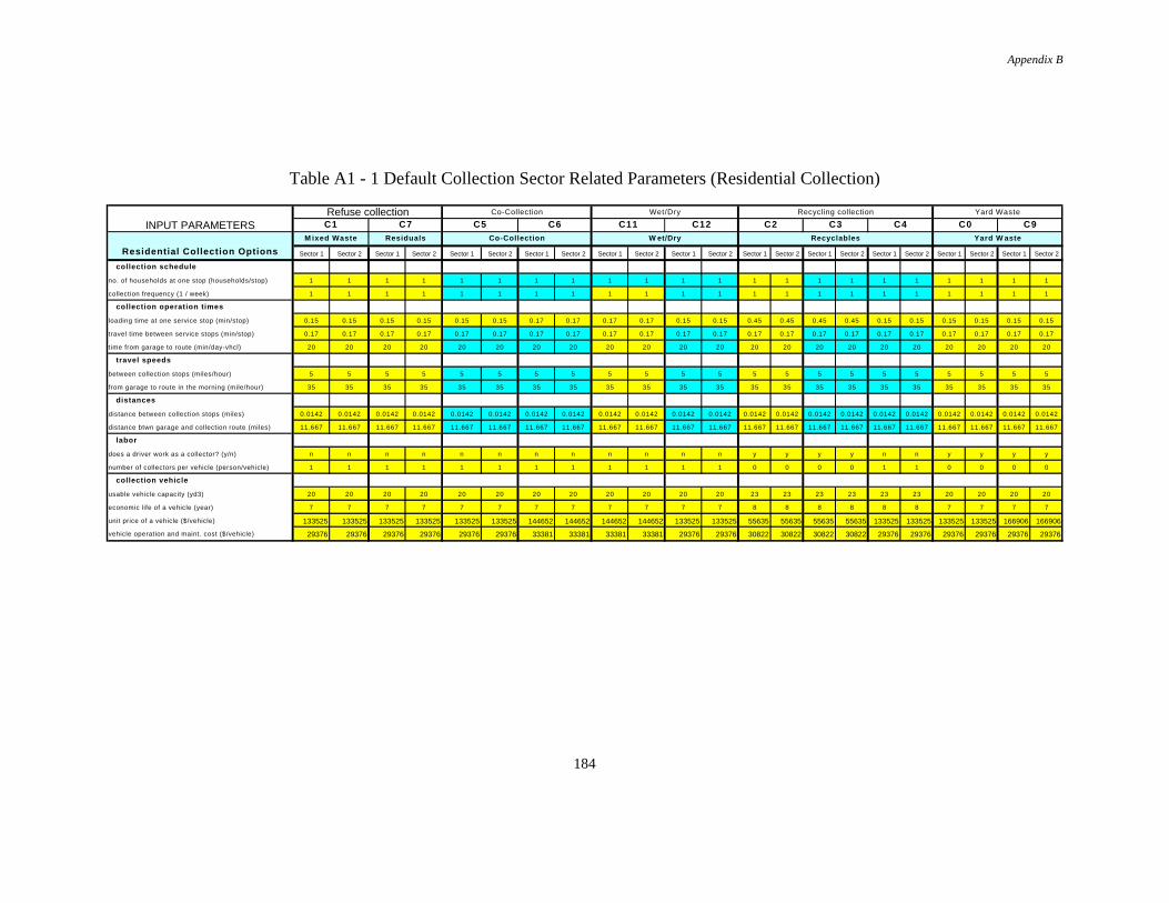
Appendix B
184
Table A1 - 1 Default Collection Sector Related Parameters (Residential Collection)
Refuse collection Co-Collection Wet/Dry Recycling collection Yard Waste
INPUT PARAMETERS C1 C7 C5 C6 C11 C12 C2 C3 C4 C0 C9M ixed Waste Residuals Co-Collection W et/Dry Recyclables Yard W aste
Residential Collection Options Sector 1 Sector 2 Sector 1 Sector 2 Sector 1 Sector 2 Sector 1 Sector 2 Sector 1 Sector 2 Sector 1 Sector 2 Sector 1 Sector 2 Sector 1 Sector 2 Sector 1 Sector 2 Sector 1 Sector 2 Sector 1 Sector 2
collection schedule
no. of households at one stop (households/stop) 1 1 1 1 1 1 1 1 1 1 1 1 1 1 1 1 1 1 1 1 1 1
collection frequency (1 / week) 1 1 1 1 1 1 1 1 1 1 1 1 1 1 1 1 1 1 1 1 1 1
collection operation times
loading time at one service stop (min/stop) 0.15 0.15 0.15 0.15 0.15 0.15 0.17 0.17 0.17 0.17 0.15 0.15 0.45 0.45 0.45 0.45 0.15 0.15 0.15 0.15 0.15 0.15
travel time between service stops (min/stop) 0.17 0.17 0.17 0.17 0.17 0.17 0.17 0.17 0.17 0.17 0.17 0.17 0.17 0.17 0.17 0.17 0.17 0.17 0.17 0.17 0.17 0.17
time from garage to route (min/day-vhcl) 20 20 20 20 20 20 20 20 20 20 20 20 20 20 20 20 20 20 20 20 20 20
travel speeds
between collection stops (miles/hour) 5 5 5 5 5 5 5 5 5 5 5 5 5 5 5 5 5 5 5 5 5 5
from garage to route in the morning (mile/hour) 35 35 35 35 35 35 35 35 35 35 35 35 35 35 35 35 35 35 35 35 35 35
distances
distance between collection stops (miles) 0.0142 0.0142 0.0142 0.0142 0.0142 0.0142 0.0142 0.0142 0.0142 0.0142 0.0142 0.0142 0.0142 0.0142 0.0142 0.0142 0.0142 0.0142 0.0142 0.0142 0.0142 0.0142
distance btwn garage and collection route (miles) 11.667 11.667 11.667 11.667 11.667 11.667 11.667 11.667 11.667 11.667 11.667 11.667 11.667 11.667 11.667 11.667 11.667 11.667 11.667 11.667 11.667 11.667
labor
does a driver work as a collector? (y/n) n n n n n n n n n n n n y y y y n n y y y y
number of collectors per vehicle (person/vehicle) 1 1 1 1 1 1 1 1 1 1 1 1 0 0 0 0 1 1 0 0 0 0
collection vehicle
usable vehicle capacity (yd3) 20 20 20 20 20 20 20 20 20 20 20 20 23 23 23 23 23 23 20 20 20 20
economic life of a vehicle (year) 7 7 7 7 7 7 7 7 7 7 7 7 8 8 8 8 8 8 7 7 7 7
unit price of a vehicle ($/vehicle) 133525 133525 133525 133525 133525 133525 144652 144652 144652 144652 133525 133525 55635 55635 55635 55635 133525 133525 133525 133525 166906 166906
vehicle operation and maint. cost ($/vehicle) 29376 29376 29376 29376 29376 29376 33381 33381 33381 33381 29376 29376 30822 30822 30822 30822 29376 29376 29376 29376 29376 29376
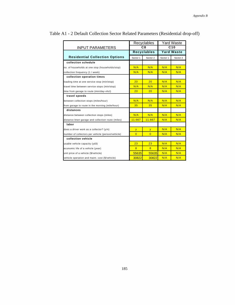
Appendix B
185
Table A1 - 2 Default Collection Sector Related Parameters (Residential drop-off)
Recyclables Yard WasteINPUT PARAMETERS C8 C10
Recyclables Yard Waste
Residential Collection Options Sector 1 Sector 2 Sector 1 Sector 2
collection schedule
no. of households at one stop (households/stop) N/A N/A N/A N/A
collection frequency (1 / week) N/A N/A N/A N/A
collection operation times
loading time at one service stop (min/stop) 20 20 N/A N/A
travel time between service stops (min/stop) N/A N/A N/A N/A
time from garage to route (min/day-vhcl) 20 20 N/A N/A
travel speeds
between collection stops (miles/hour) N/A N/A N/A N/A
from garage to route in the morning (mile/hour) 35 35 N/A N/A
distances
distance between collection stops (miles) N/A N/A N/A N/A
distance btwn garage and collection route (miles) 11.667 11.667 N/A N/A
labor
does a driver work as a collector? (y/n) y y N/A N/A
number of collectors per vehicle (person/vehicle) 0 0 N/A N/A
collection vehicle
usable vehicle capacity (yd3) 23 23 N/A N/A
economic life of a vehicle (year) 8 8 N/A N/A
unit price of a vehicle ($/vehicle) 55635 55635 N/A N/A
vehicle operation and maint. cost ($/vehicle) 30822 30822 N/A N/A
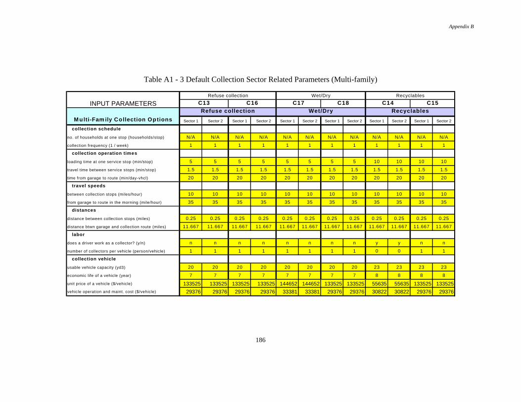
Appendix B
186
Table A1 - 3 Default Collection Sector Related Parameters (Multi-family)
Refuse collection Wet/Dry Recyclables
INPUT PARAMETERS C13 C16 C17 C18 C14 C15Refuse collection Wet/Dry Recyclables
Multi-Fam ily Collection Options Sector 1 Sector 2 Sector 1 Sector 2 Sector 1 Sector 2 Sector 1 Sector 2 Sector 1 Sector 2 Sector 1 Sector 2
collection schedule
no. of households at one stop (households/stop) N/A N/A N/A N/A N/A N/A N/A N/A N/A N/A N/A N/A
collection frequency (1 / week) 1 1 1 1 1 1 1 1 1 1 1 1
collection operation times
loading time at one service stop (min/stop) 5 5 5 5 5 5 5 5 10 10 10 10
travel time between service stops (min/stop) 1.5 1.5 1.5 1.5 1.5 1.5 1.5 1.5 1.5 1.5 1.5 1.5
time from garage to route (min/day-vhcl) 20 20 20 20 20 20 20 20 20 20 20 20
travel speeds
between collection stops (miles/hour) 10 10 10 10 10 10 10 10 10 10 10 10
from garage to route in the morning (mile/hour) 35 35 35 35 35 35 35 35 35 35 35 35
distances
distance between collection stops (miles) 0.25 0.25 0.25 0.25 0.25 0.25 0.25 0.25 0.25 0.25 0.25 0.25
distance btwn garage and collection route (miles) 11.667 11.667 11.667 11.667 11.667 11.667 11.667 11.667 11.667 11.667 11.667 11.667
labor
does a driver work as a collector? (y/n) n n n n n n n n y y n n
number of collectors per vehicle (person/vehicle) 1 1 1 1 1 1 1 1 0 0 1 1
collection vehicle
usable vehicle capacity (yd3) 20 20 20 20 20 20 20 20 23 23 23 23
economic life of a vehicle (year) 7 7 7 7 7 7 7 7 8 8 8 8
unit price of a vehicle ($/vehicle) 133525 133525 133525 133525 144652 144652 133525 133525 55635 55635 133525 133525vehicle operation and maint. cost ($/vehicle) 29376 29376 29376 29376 33381 33381 29376 29376 30822 30822 29376 29376
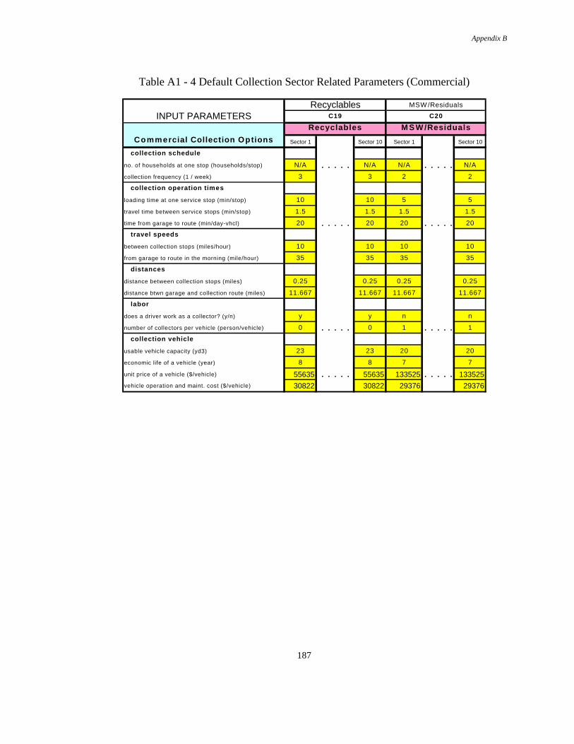
Appendix B
187
Table A1 - 4 Default Collection Sector Related Parameters (Commercial)
Recyclables MSW /Residuals
INPUT PARAMETERS C19 C20
Recyclables M S W /Residuals
Commercial Collection Options Sector 1 Sector 10 Sector 1 Sector 10
collection schedule
no. of households at one stop (households/stop) N/A . . . . . N/A N/A . . . . . N/A
collection frequency (1 / week) 3 3 2 2
collection operation times
loading time at one service stop (min/stop) 10 10 5 5
travel time between service stops (min/stop) 1.5 1.5 1.5 1.5
time from garage to route (min/day-vhcl) 20 . . . . . 20 20 . . . . . 20
travel speeds
between collection stops (miles/hour) 10 10 10 10
from garage to route in the morning (mile/hour) 35 35 35 35
distances
distance between collection stops (miles) 0.25 0.25 0.25 0.25
distance btwn garage and collection route (miles) 11.667 11.667 11.667 11.667
labor
does a driver work as a collector? (y/n) y y n n
number of collectors per vehicle (person/vehicle) 0 . . . . . 0 1 . . . . . 1
collection vehicle
usable vehicle capacity (yd3) 23 23 20 20
economic life of a vehicle (year) 8 8 7 7
unit price of a vehicle ($/vehicle) 55635 . . . . . 55635 133525 . . . . . 133525vehicle operation and maint. cost ($/vehicle) 30822 30822 29376 29376
Appendix C
188
APPENDIX C
DEFAULT INPUT VALUES(FOR VARIABLES WITH SECTOR AND NEXT NODE
VARIABILITY)
Appendix C
189
Solid vertical lines are used in the printout to separate collection options into sets ofoptions that are similar to each other. Lightly shaded cells represent input variableswhich might be expected to have a unique value for the option in which the shaded cellappears. Darkly shaded cells represent input variables that are used in the area of thespreadsheet shown, but which are entered in some other location in the process model.
It should be noted that several of the collection options for which distances tounloading could be expected to be the same have been grouped to prevent the necessityfor the user entering these distances more than once. Collection Options in Group 1include C1, C7, C5, C6, C11 and C12 while group 2 collection options include C2, C3,and C4. These collection options are similar enough that the garage would be located inthe same place regardless of which collection options are implemented and materialcollected via these options could be expected to flow to the same locations.

Appendix C
190
Table C2 - 1 Default Collection Distances to Next MSW Node
Relative to Node TRAVEL PARAMETER UNITSSector 10
Group 1 Group 2 C17/ C0 C9 C8 Group 1 Group 2 C17/ C0 C9 C8 C17/ All C17/ All C19 C20 C19 C20
C18 C18 C18 Others C18 Others
btwn collection route and facility Miles 11.00 11.00 15.00 10.00 10.00 15.00 12.00 12.00 15.00 12.00 12.00 12.00 15.00 10.00 15.00 12.00 10.00 10.00 10.00 10.00
between facil i ty and garage Miles 13.00 13.00 14.00 11.67 11.67 11.67 14.00 14.00 14.00 14.00 14.00 14.00 14.00 11.67 14.00 14.00 11.67 11.67 11.67 11.67
btwn collection route and facility Miles/Hour 30.00 30.00 30.00 30.00 30.00 30.00 31.00 31.00 30.00 31.00 31.00 31.00 30.00 30.00 30.00 31.00 30.00 30.00 30.00 30.00
between facil i ty and garage Miles/Hour 35.00 35.00 35.00 35.00 35.00 35.00 36.00 36.00 35.00 36.00 36.00 36.00 35.00 35.00 35.00 36.00 35.00 35.00 35.00 35.00
t ime btwn facil ity and garage Min/Day-Vech. 20.00 20.00 20.00 20.00 20.00 20.00 20.00 20.00 20.00 20.00 20.00 20.00 20.00 20.00 20.00 20.00 20.00 20.00 20.00 20.00
t ime btwn route and facil ity Min/Trip 20.00 20.00 20.00 20.00 20.00 20.00 20.00 20.00 20.00 20.00 20.00 20.00 20.00 20.00 20.00 20.00 20.00 20.00 20.00 20.00
btwn collection route and facility Miles 11.00 11.00 15.00 10.00 10.00 15.00 12.00 12.00 15.00 12.00 12.00 12.00 15.00 10.00 15.00 12.00 0.00 0.00 0.00 0.00
between facil i ty and garage Miles 13.00 13.00 14.00 11.67 11.67 11.67 14.00 14.00 14.00 14.00 14.00 14.00 14.00 11.67 14.00 14.00 0.00 0.00 0.00 0.00
btwn collection route and facility Miles/Hour 30.00 30.00 30.00 30.00 30.00 30.00 31.00 31.00 30.00 31.00 31.00 31.00 30.00 30.00 30.00 31.00 0.00 0.00 0.00 0.00
between facil i ty and garage Miles/Hour 35.00 35.00 35.00 35.00 35.00 35.00 36.00 36.00 35.00 36.00 36.00 36.00 35.00 35.00 35.00 36.00 0.00 0.00 0.00 0.00
t ime btwn facil ity and garage Min/Day-Vech. 20.00 20.00 20.00 20.00 20.00 20.00 20.00 20.00 20.00 20.00 20.00 20.00 20.00 20.00 20.00 20.00 0.00 0.00 0.00 0.00
t ime btwn route and facil ity Min/Trip 20.00 20.00 20.00 20.00 20.00 20.00 20.00 20.00 20.00 20.00 20.00 20.00 20.00 20.00 20.00 20.00 0.00 0.00 0.00 0.00
btwn collection route and facility Miles 11.00 11.00 15.00 10.00 10.00 15.00 12.00 12.00 15.00 12.00 12.00 12.00 15.00 10.00 15.00 12.00 10.00 10.00 10.00 10.00
between facil i ty and garage Miles 13.00 13.00 14.00 11.67 11.67 11.67 14.00 14.00 14.00 14.00 14.00 14.00 14.00 11.67 14.00 14.00 11.67 11.67 11.67 11.67
btwn collection route and facility Miles/Hour 30.00 30.00 30.00 30.00 30.00 30.00 31.00 31.00 30.00 31.00 31.00 31.00 30.00 30.00 30.00 31.00 30.00 30.00 30.00 30.00
between facil i ty and garage Miles/Hour 35.00 35.00 35.00 35.00 35.00 35.00 36.00 36.00 35.00 36.00 36.00 36.00 35.00 35.00 35.00 36.00 35.00 35.00 35.00 35.00
t ime btwn facil ity and garage Min/Day-Vech. 20.00 20.00 20.00 20.00 20.00 20.00 20.00 20.00 20.00 20.00 20.00 20.00 20.00 20.00 20.00 20.00 20.00 20.00 20.00 20.00
t ime btwn route and facil ity Min/Trip 20.00 20.00 20.00 20.00 20.00 20.00 20.00 20.00 20.00 20.00 20.00 20.00 20.00 20.00 20.00 20.00 20.00 20.00 20.00 20.00
. . . . .
. . . . .
. . . . .
. . . . .
. . . . .
. . . . .
Residential M u lti-Fam ily
Sector 1 Sector 2 Sector 1 Sector 2
Mixed Refuse MRF (S1)
Pre-Sorted Transfer Station (TR5)
Co-collected Transfer Station (TR4)
Co-collected Transfer Station (TR3)
Commingled Recyclables Transfer (TR2)
Mixed Refuse Transfer (TR1)
Rail Transfer (RT1)
Commercial
. . . . .
Sector 1

Appendix C
191
Table C2 - 2 Default Collection Distances to Next MSW Node (Continued)
btwn collection route and facility Miles 11.00 11.00 15.00 10.00 10.00 15.00 12.00 12.00 15.00 12.00 12.00 12.00 15.00 10.00 15.00 12.00 10.00 10.00 10.00 10.00
between facility and garage Miles 13.00 13.00 14.00 11.67 11.67 11.67 14.00 14.00 14.00 14.00 14.00 14.00 14.00 11.67 14.00 14.00 11.67 11.67 11.67 11.67
btwn collection route and facility Miles/Hour 30.00 30.00 30.00 30.00 30.00 30.00 31.00 31.00 30.00 31.00 31.00 31.00 30.00 30.00 30.00 31.00 30.00 30.00 30.00 30.00
between facility and garage Miles/Hour 35.00 35.00 35.00 35.00 35.00 35.00 36.00 36.00 35.00 36.00 36.00 36.00 35.00 35.00 35.00 36.00 35.00 35.00 35.00 35.00
time btwn facility and garage Min/Day-Vech. 20.00 20.00 20.00 20.00 20.00 20.00 20.00 20.00 20.00 20.00 20.00 20.00 20.00 20.00 20.00 20.00 20.00 20.00 20.00 20.00
time btwn route and facility Min/Trip 20.00 20.00 20.00 20.00 20.00 20.00 20.00 20.00 20.00 20.00 20.00 20.00 20.00 20.00 20.00 20.00 20.00 20.00 20.00 20.00
btwn collection route and facility Miles 11.00 11.00 15.00 10.00 10.00 15.00 12.00 12.00 15.00 12.00 12.00 12.00 15.00 10.00 15.00 12.00 0.00 0.00 0.00 0.00
between facility and garage Miles 13.00 13.00 14.00 11.67 11.67 11.67 14.00 14.00 14.00 14.00 14.00 14.00 14.00 11.67 14.00 14.00 0.00 0.00 0.00 0.00
btwn collection route and facility Miles/Hour 30.00 30.00 30.00 30.00 30.00 30.00 31.00 31.00 30.00 31.00 31.00 31.00 30.00 30.00 30.00 31.00 0.00 0.00 0.00 0.00
between facility and garage Miles/Hour 35.00 35.00 35.00 35.00 35.00 35.00 36.00 36.00 35.00 36.00 36.00 36.00 35.00 35.00 35.00 36.00 0.00 0.00 0.00 0.00
time btwn facility and garage Min/Day-Vech. 20.00 20.00 20.00 20.00 20.00 20.00 20.00 20.00 20.00 20.00 20.00 20.00 20.00 20.00 20.00 20.00 0.00 0.00 0.00 0.00
time btwn route and facility Min/Trip 20.00 20.00 20.00 20.00 20.00 20.00 20.00 20.00 20.00 20.00 20.00 20.00 20.00 20.00 20.00 20.00 0.00 0.00 0.00 0.00
btwn collection route and facility Miles 11.00 11.00 15.00 10.00 10.00 15.00 12.00 12.00 15.00 12.00 12.00 12.00 15.00 0.00 0.00 0.00 0.00 0.00 0.00 0.00
between facility and garage Miles 13.00 13.00 14.00 11.67 11.67 11.67 14.00 14.00 14.00 14.00 14.00 14.00 14.00 0.00 0.00 0.00 0.00 0.00 0.00 0.00
btwn collection route and facility Miles/Hour 30.00 30.00 30.00 30.00 30.00 30.00 31.00 31.00 30.00 31.00 31.00 31.00 30.00 0.00 0.00 0.00 0.00 0.00 0.00 0.00
between facility and garage Miles/Hour 35.00 35.00 35.00 35.00 35.00 35.00 36.00 36.00 35.00 36.00 36.00 36.00 35.00 0.00 0.00 0.00 0.00 0.00 0.00 0.00
time btwn facility and garage Min/Day-Vech. 20.00 20.00 20.00 20.00 20.00 20.00 20.00 20.00 20.00 20.00 20.00 20.00 20.00 0.00 0.00 0.00 0.00 0.00 0.00 0.00
time btwn route and facility Min/Trip 20.00 20.00 20.00 20.00 20.00 20.00 20.00 20.00 20.00 20.00 20.00 20.00 20.00 0.00 0.00 0.00 0.00 0.00 0.00 0.00
btwn collection route and facility Miles 11.00 11.00 15.00 10.00 10.00 15.00 12.00 12.00 15.00 12.00 12.00 12.00 15.00 10.00 15.00 12.00 10.00 10.00 10.00 10.00
between facility and garage Miles 13.00 13.00 14.00 11.67 11.67 11.67 14.00 14.00 14.00 14.00 14.00 14.00 14.00 11.67 14.00 14.00 11.67 11.67 11.67 11.67
btwn collection route and facility Miles/Hour 30.00 30.00 30.00 30.00 30.00 30.00 31.00 31.00 30.00 31.00 31.00 31.00 30.00 30.00 30.00 31.00 30.00 30.00 30.00 30.00
between facility and garage Miles/Hour 35.00 35.00 35.00 35.00 35.00 35.00 36.00 36.00 35.00 36.00 36.00 36.00 35.00 35.00 35.00 36.00 35.00 35.00 35.00 35.00
time btwn facility and garage Min/Day-Vech. 20.00 20.00 20.00 20.00 20.00 20.00 20.00 20.00 20.00 20.00 20.00 20.00 20.00 20.00 20.00 20.00 20.00 20.00 20.00 20.00
time btwn route and facility Min/Trip 20.00 20.00 20.00 20.00 20.00 20.00 20.00 20.00 20.00 20.00 20.00 20.00 20.00 20.00 20.00 20.00 20.00 20.00 20.00 20.00
. . . . .
. . . . .
. . . . .
. . . . .
. . . . .
. . . . .
. . . . .
Yard W aste Composting (T1)
Combustion (T3)
Commingled Recyclables (S3)
Pre-sorted MRF (S2)
RDF (T5)
Commingled Recyclables (bags, 1 compartment) (S4)
Commingled Recyclables
(bags, 2 compartment) (S5)

Appendix C
192
Table C2 - 3 Default Collection Distances to Next MSW Node (Continued)
btwn collection route and facility Miles 11.00 11.00 15.00 10.00 10.00 15.00 12.00 12.00 15.00 12.00 12.00 12.00 15.00 10.00 15.00 12.00 10.00 10.00 10.00 10.00
between facility and garage Miles 13.00 13.00 14.00 11.67 11.67 11.67 14.00 14.00 14.00 14.00 14.00 14.00 14.00 11.67 14.00 14.00 11.67 11.67 11.67 11.67
btwn collection route and facility Miles/Hour 30.00 30.00 30.00 30.00 30.00 30.00 31.00 31.00 30.00 31.00 31.00 31.00 30.00 30.00 30.00 31.00 30.00 30.00 30.00 30.00
between facility and garage Miles/Hour 35.00 35.00 35.00 35.00 35.00 35.00 36.00 36.00 35.00 36.00 36.00 36.00 35.00 35.00 35.00 36.00 35.00 35.00 35.00 35.00
time btwn facility and garage Min/Day-Vech. 20.00 20.00 20.00 20.00 20.00 20.00 20.00 20.00 20.00 20.00 20.00 20.00 20.00 20.00 20.00 20.00 20.00 20.00 20.00 20.00
time btwn route and facility Min/Trip 20.00 20.00 20.00 20.00 20.00 20.00 20.00 20.00 20.00 20.00 20.00 20.00 20.00 20.00 20.00 20.00 20.00 20.00 20.00 20.00
btwn collection route and facility Miles 11.00 11.00 15.00 10.00 10.00 15.00 12.00 12.00 15.00 12.00 12.00 12.00 15.00 0.00 0.00 0.00 0.00 0.00 0.00 0.00
between facility and garage Miles 13.00 13.00 14.00 11.67 11.67 11.67 14.00 14.00 14.00 14.00 14.00 14.00 14.00 0.00 0.00 0.00 0.00 0.00 0.00 0.00
btwn collection route and facility Miles/Hour 30.00 30.00 30.00 30.00 30.00 30.00 31.00 31.00 30.00 31.00 31.00 31.00 30.00 0.00 0.00 0.00 0.00 0.00 0.00 0.00
between facility and garage Miles/Hour 35.00 35.00 35.00 35.00 35.00 35.00 36.00 36.00 35.00 36.00 36.00 36.00 35.00 0.00 0.00 0.00 0.00 0.00 0.00 0.00
time btwn facility and garage Min/Day-Vech. 20.00 20.00 20.00 20.00 20.00 20.00 20.00 20.00 20.00 20.00 20.00 20.00 20.00 0.00 0.00 0.00 0.00 0.00 0.00 0.00
time btwn route and facility Min/Trip 20.00 20.00 20.00 20.00 20.00 20.00 20.00 20.00 20.00 20.00 20.00 20.00 20.00 0.00 0.00 0.00 0.00 0.00 0.00 0.00
. . . . .
. . . . .
. . . . .
. . . . .
. . . . .
Enhanced Bioreactor (D3)
W aste as Fuel (Leaves)
Mixed Waste Composting
(T7)
Anaerobic Digestion (T8)
Landfill (D1)
Appendix D
193
APPENDIX D
SAMPLE OUTPUT
Appendix D
194
The following pages show a printout of Collection Preprocessor output generatedfrom the default input values shown in Appendix A.
Note that the values for “number of collection vehicles” and “Total annual cost” forrecyclables collection options C3, C4, C8, and C15 and yard waste collection option C9are zero. This occurred because the default inputs include zero values for the fraction ofthe community served (option_frac) by these collection options. Only one residentialrecyclables collection option (C2) and one yard waste collection option (C0) wereassigned non-zero option_frac values. Option_frac for both C2 and C0 is 100%. Thissatisfies the requirement that the sum of the fractions of the community served bydifferent recyclable or yard waste options not exceed 100%.
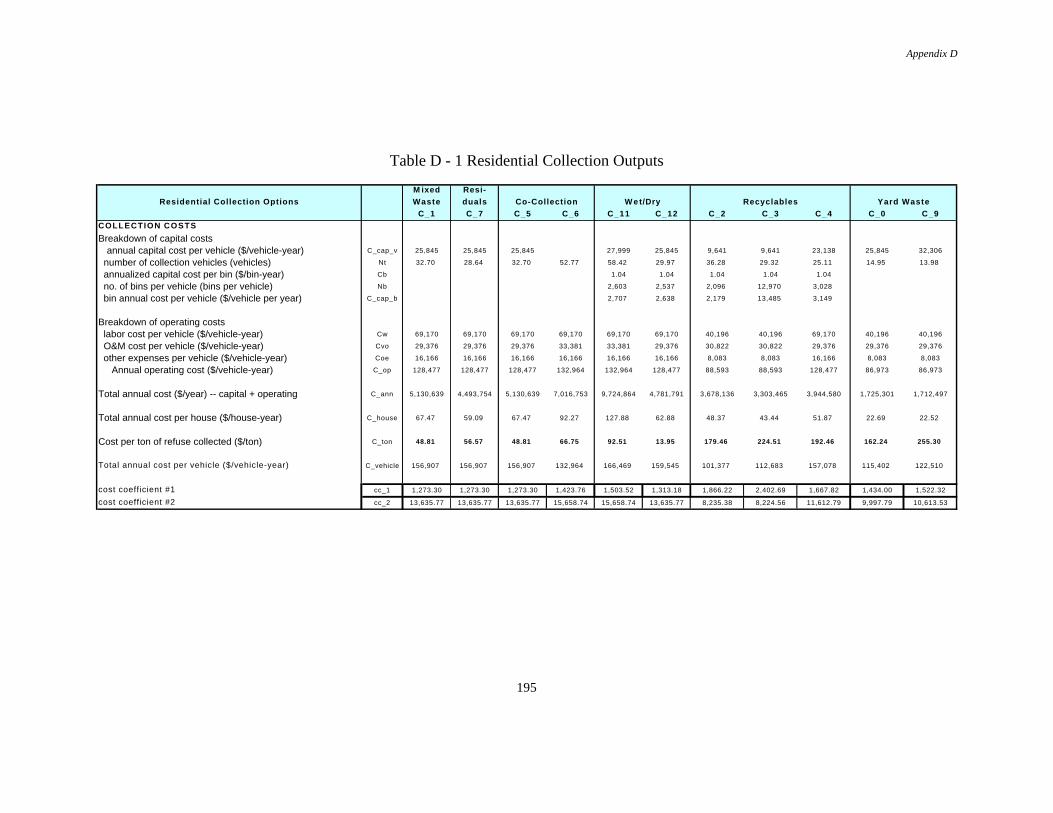
Appendix D
195
Table D - 1 Residential Collection Outputs
M ixed Resi-
Residential Collection Options Waste duals Co-Collection W e t/Dry Recyclables Yard Waste
C_1 C_7 C_5 C_6 C_11 C_12 C_2 C_3 C_4 C_0 C_9
COLLECTION COSTS
Breakdown of capital costs annual capital cost per vehicle ($/vehicle-year) C_cap_v 25,845 25,845 25,845 27,999 25,845 9,641 9,641 23,138 25,845 32,306
number of collection vehicles (vehicles) Nt 32.70 28.64 32.70 52.77 58.42 29.97 36.28 29.32 25.11 14.95 13.98
annualized capital cost per bin ($/bin-year) Cb 1.04 1.04 1.04 1.04 1.04
no. of bins per vehicle (bins per vehicle) Nb 2,603 2,537 2,096 12,970 3,028
bin annual cost per vehicle ($/vehicle per year) C_cap_b 2,707 2,638 2,179 13,485 3,149
Breakdown of operating costs labor cost per vehicle ($/vehicle-year) Cw 69,170 69,170 69,170 69,170 69,170 69,170 40,196 40,196 69,170 40,196 40,196
O&M cost per vehicle ($/vehicle-year) Cvo 29,376 29,376 29,376 33,381 33,381 29,376 30,822 30,822 29,376 29,376 29,376
other expenses per vehicle ($/vehicle-year) Coe 16,166 16,166 16,166 16,166 16,166 16,166 8,083 8,083 16,166 8,083 8,083
Annual operating cost ($/vehicle-year) C_op 128,477 128,477 128,477 132,964 132,964 128,477 88,593 88,593 128,477 86,973 86,973
Total annual cost ($/year) -- capital + operating C_ann 5,130,639 4,493,754 5,130,639 7,016,753 9,724,864 4,781,791 3,678,136 3,303,465 3,944,580 1,725,301 1,712,497
Total annual cost per house ($/house-year) C_house 67.47 59.09 67.47 92.27 127.88 62.88 48.37 43.44 51.87 22.69 22.52
Cost per ton of refuse collected ($/ton) C_ton 48.81 56.57 48.81 66.75 92.51 13.95 179.46 224.51 192.46 162.24 255.30
Total annual cost per vehicle ($/vehicle-year) C_vehicle 156,907 156,907 156,907 132,964 166,469 159,545 101,377 112,683 157,078 115,402 122,510
cost coefficient #1 cc_1 1,273.30 1,273.30 1,273.30 1,423.76 1,503.52 1,313.18 1,866.22 2,402.69 1,667.82 1,434.00 1,522.32
cost coefficient #2 cc_2 13,635.77 13,635.77 13,635.77 15,658.74 15,658.74 13,635.77 8,235.38 8,224.56 11,612.79 9,997.79 10,613.53
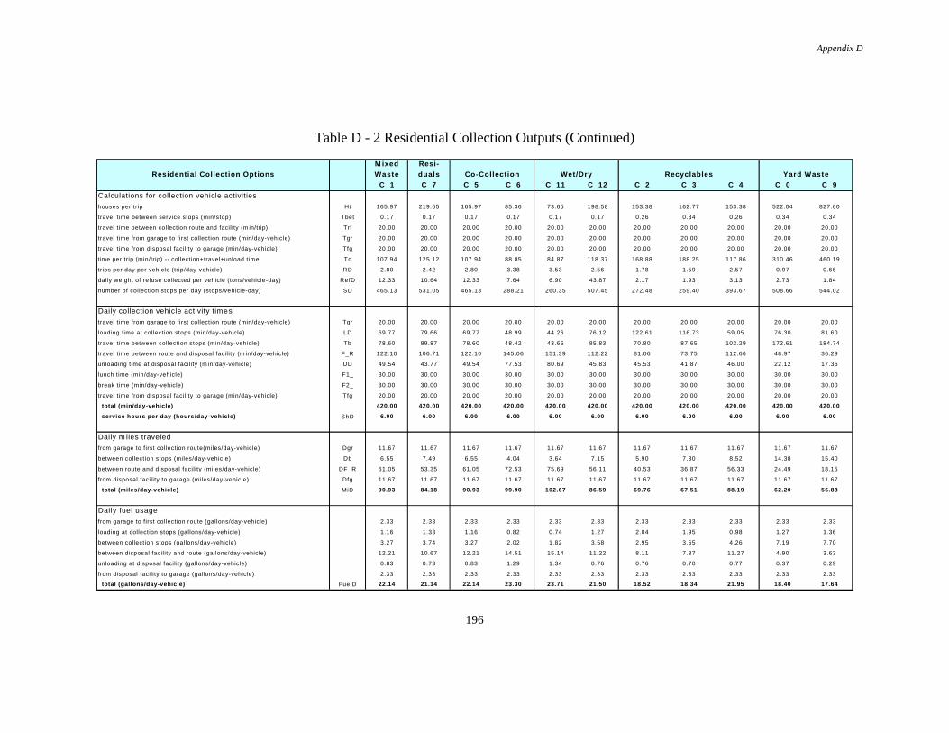
Appendix D
196
Table D - 2 Residential Collection Outputs (Continued)
M ixed Resi-
Residential Collection Options Waste duals Co-Collection Wet/Dry Recyclables Yard Waste
C_1 C_7 C_5 C_6 C_11 C_12 C_2 C_3 C_4 C_0 C_9
Calculations for collection vehicle activities
houses per trip Ht 165.97 219.65 165.97 85.36 73.65 198.58 153.38 162.77 153.38 522.04 827.60
travel time between service stops (min/stop) Tbet 0.17 0.17 0.17 0.17 0.17 0.17 0.26 0.34 0.26 0.34 0.34
travel time between collection route and facility (m in/trip) Trf 20.00 20.00 20.00 20.00 20.00 20.00 20.00 20.00 20.00 20.00 20.00
travel time from garage to first collection route (min/day-vehicle) Tgr 20.00 20.00 20.00 20.00 20.00 20.00 20.00 20.00 20.00 20.00 20.00
travel time from disposal facility to garage (min/day-vehicle) Tfg 20.00 20.00 20.00 20.00 20.00 20.00 20.00 20.00 20.00 20.00 20.00
time per trip (min/trip) -- collection+travel+unload time Tc 107.94 125.12 107.94 88.85 84.87 118.37 168.88 188.25 117.86 310.46 460.19
trips per day per vehicle (trip/day-vehicle) RD 2.80 2.42 2.80 3.38 3.53 2.56 1.78 1.59 2.57 0.97 0.66
daily weight of refuse collected per vehicle (tons/vehicle-day) RefD 12.33 10.64 12.33 7.64 6.90 43.87 2.17 1.93 3.13 2.73 1.84
number of collection stops per day (stops/vehicle-day) SD 465.13 531.05 465.13 288.21 260.35 507.45 272.48 259.40 393.67 508.66 544.02
Daily collection vehicle activity times
travel time from garage to first collection route (min/day-vehicle) Tgr 20.00 20.00 20.00 20.00 20.00 20.00 20.00 20.00 20.00 20.00 20.00
loading time at collection stops (min/day-vehicle) LD 69.77 79.66 69.77 48.99 44.26 76.12 122.61 116.73 59.05 76.30 81.60
travel time between collection stops (min/day-vehicle) Tb 78.60 89.87 78.60 48.42 43.66 85.83 70.80 87.65 102.29 172.61 184.74
travel time between route and disposal facility (m in/day-vehicle) F_R 122.10 106.71 122.10 145.06 151.39 112.22 81.06 73.75 112.66 48.97 36.29
unloading time at disposal facility (m in/day-vehicle) UD 49.54 43.77 49.54 77.53 80.69 45.83 45.53 41.87 46.00 22.12 17.36
lunch time (min/day-vehicle) F1_ 30.00 30.00 30.00 30.00 30.00 30.00 30.00 30.00 30.00 30.00 30.00
break time (min/day-vehicle) F2_ 30.00 30.00 30.00 30.00 30.00 30.00 30.00 30.00 30.00 30.00 30.00
travel time from disposal facility to garage (min/day-vehicle) Tfg 20.00 20.00 20.00 20.00 20.00 20.00 20.00 20.00 20.00 20.00 20.00
total (min/day-vehicle) 420.00 420.00 420.00 420.00 420.00 420.00 420.00 420.00 420.00 420.00 420.00
service hours per day (hours/day-vehicle) ShD 6.00 6.00 6.00 6.00 6.00 6.00 6.00 6.00 6.00 6.00 6.00
Daily m iles traveledfrom garage to first collection route(miles/day-vehicle) Dgr 11.67 11.67 11.67 11.67 11.67 11.67 11.67 11.67 11.67 11.67 11.67
between collection stops (miles/day-vehicle) Db 6.55 7.49 6.55 4.04 3.64 7.15 5.90 7.30 8.52 14.38 15.40
between route and disposal facility (miles/day-vehicle) DF_R 61.05 53.35 61.05 72.53 75.69 56.11 40.53 36.87 56.33 24.49 18.15
from disposal facility to garage (miles/day-vehicle) Dfg 11.67 11.67 11.67 11.67 11.67 11.67 11.67 11.67 11.67 11.67 11.67
total (miles/day-vehicle) MiD 90.93 84.18 90.93 99.90 102.67 86.59 69.76 67.51 88.19 62.20 56.88
Daily fuel usage
from garage to first collection route (gallons/day-vehicle) 2.33 2.33 2.33 2.33 2.33 2.33 2.33 2.33 2.33 2.33 2.33
loading at collection stops (gallons/day-vehicle) 1.16 1.33 1.16 0.82 0.74 1.27 2.04 1.95 0.98 1.27 1.36
between collection stops (gallons/day-vehicle) 3.27 3.74 3.27 2.02 1.82 3.58 2.95 3.65 4.26 7.19 7.70
between disposal facility and route (gallons/day-vehicle) 12.21 10.67 12.21 14.51 15.14 11.22 8.11 7.37 11.27 4.90 3.63
unloading at disposal facility (gallons/day-vehicle) 0.83 0.73 0.83 1.29 1.34 0.76 0.76 0.70 0.77 0.37 0.29
from disposal facility to garage (gallons/day-vehicle) 2.33 2.33 2.33 2.33 2.33 2.33 2.33 2.33 2.33 2.33 2.33
total (gallons/day-vehicle) FuelD 22.14 21.14 22.14 23.30 23.71 21.50 18.52 18.34 21.95 18.40 17.64
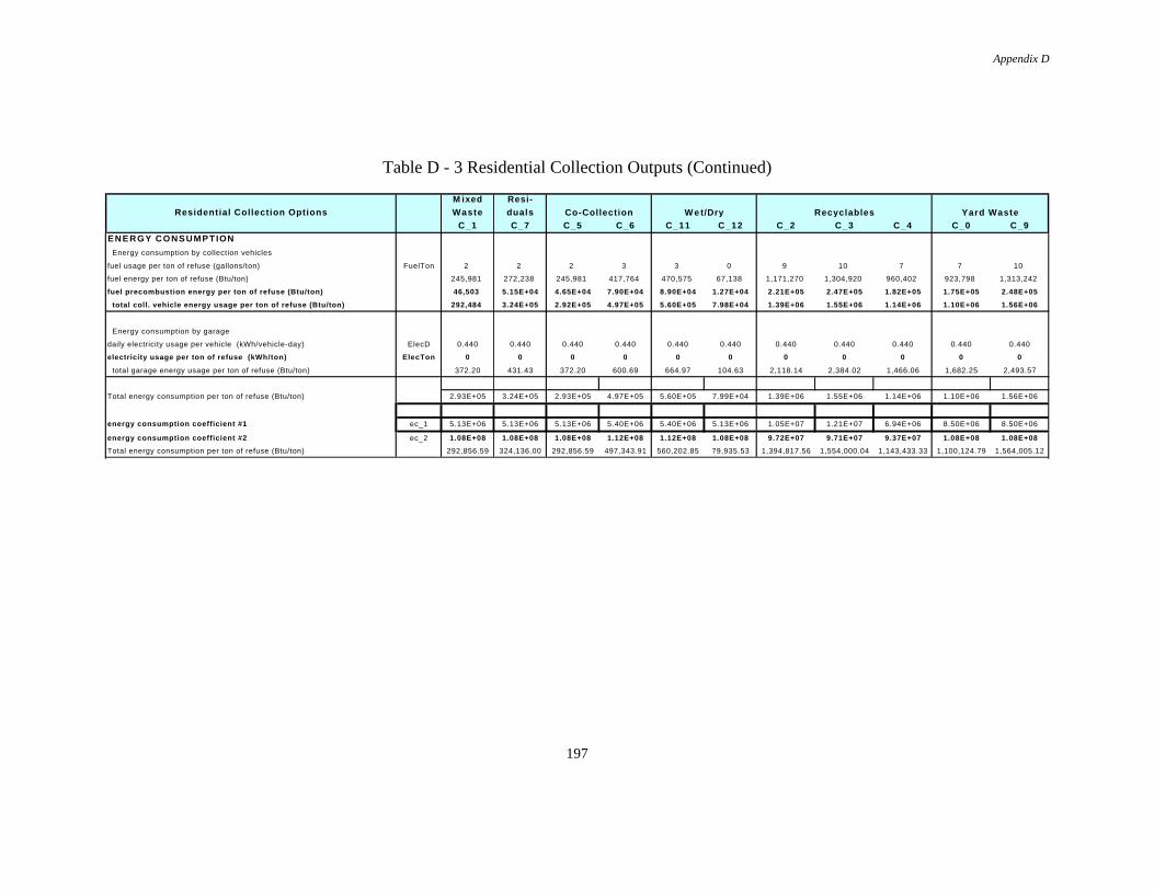
Appendix D
197
Table D - 3 Residential Collection Outputs (Continued)
M ixed Resi-
Residential Collection Options Waste duals
C_1 C_7 C_5 C_6 C_11 C_12 C_2 C_3 C_4 C_0 C_9
ENERGY CONSUMPTION
Energy consumption by collection vehicles
fuel usage per ton of refuse (gallons/ton) FuelTon 2 2 2 3 3 0 9 10 7 7 10
fuel energy per ton of refuse (Btu/ton) 245,981 272,238 245,981 417,764 470,575 67,138 1,171,270 1,304,920 960,402 923,798 1,313,242
fuel precombustion energy per ton of refuse (Btu/ton) 46,503 5.15E+04 4.65E+04 7.90E+04 8.90E+04 1.27E+04 2.21E+05 2.47E+05 1.82E+05 1.75E+05 2.48E+05
total coll. vehicle energy usage per ton of refuse (Btu/ton) 292,484 3.24E+05 2.92E+05 4.97E+05 5.60E+05 7.98E+04 1.39E+06 1.55E+06 1.14E+06 1.10E+06 1.56E+06
Energy consumption by garage
daily electricity usage per vehicle (kWh/vehicle-day) ElecD 0.440 0.440 0.440 0.440 0.440 0.440 0.440 0.440 0.440 0.440 0.440
electricity usage per ton of refuse (kWh/ton) ElecTon 0 0 0 0 0 0 0 0 0 0 0
total garage energy usage per ton of refuse (Btu/ton) 372.20 431.43 372.20 600.69 664.97 104.63 2,118.14 2,384.02 1,466.06 1,682.25 2,493.57
Total energy consumption per ton of refuse (Btu/ton) 2.93E+05 3.24E+05 2.93E+05 4.97E+05 5.60E+05 7.99E+04 1.39E+06 1.55E+06 1.14E+06 1.10E+06 1.56E+06
energy consumption coefficient #1 ec_1 5.13E+06 5.13E+06 5.13E+06 5.40E+06 5.40E+06 5.13E+06 1.05E+07 1.21E+07 6.94E+06 8.50E+06 8.50E+06
energy consumption coefficient #2 ec_2 1.08E+08 1.08E+08 1.08E+08 1.12E+08 1.12E+08 1.08E+08 9.72E+07 9.71E+07 9.37E+07 1.08E+08 1.08E+08
Total energy consumption per ton of refuse (Btu/ton) 292,856.59 324,136.00 292,856.59 497,343.91 560,202.85 79,935.53 1,394,817.56 1,554,000.04 1,143,433.33 1,100,124.79 1,564,005.12
Co-Collection W e t/Dry Recyclables Yard Waste
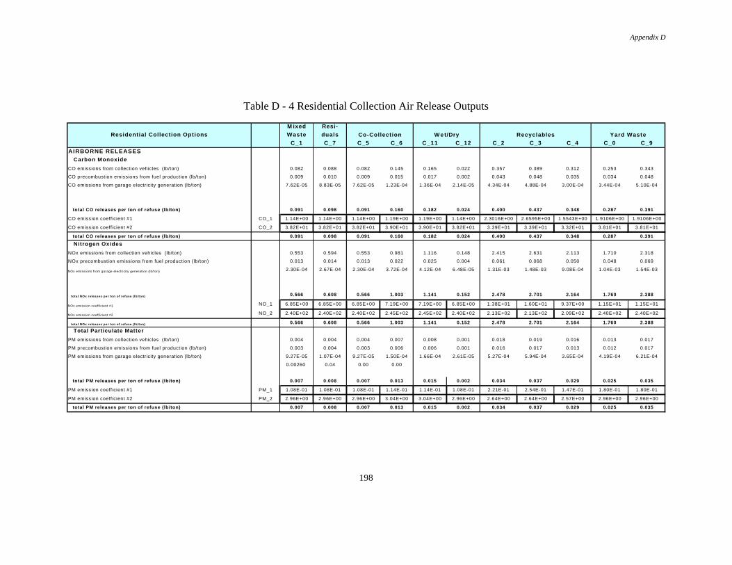
Appendix D
198
Table D - 4 Residential Collection Air Release Outputs
M ixed Resi-
Residential Collection Options Waste duals
C_1 C_7 C_5 C_6 C_11 C_12 C_2 C_3 C_4 C_0 C_9
AIRBORNE RELEASES
Carbon Monoxide
CO emissions from collection vehicles (lb/ton) 0.082 0.088 0.082 0.145 0.165 0.022 0.357 0.389 0.312 0.253 0.343
CO precombustion emissions from fuel production (lb/ton) 0.009 0.010 0.009 0.015 0.017 0.002 0.043 0.048 0.035 0.034 0.048
CO emissions from garage electricity generation (lb/ton) 7.62E-05 8.83E-05 7.62E-05 1.23E-04 1.36E-04 2.14E-05 4.34E-04 4.88E-04 3.00E-04 3.44E-04 5.10E-04
total CO releases per ton of refuse (lb/ton) 0.091 0.098 0.091 0.160 0.182 0.024 0.400 0.437 0.348 0.287 0.391
CO emission coefficient #1 CO_1 1.14E+00 1.14E+00 1.14E+00 1.19E+00 1.19E+00 1.14E+00 2.3016E+00 2.6595E+00 1.5543E+00 1.9106E+00 1.9106E+00
CO emission coefficient #2 CO_2 3.82E+01 3.82E+01 3.82E+01 3.90E+01 3.90E+01 3.82E+01 3.39E+01 3.39E+01 3.32E+01 3.81E+01 3.81E+01
total CO releases per ton of refuse (lb/ton) 0.091 0.098 0.091 0.160 0.182 0.024 0.400 0.437 0.348 0.287 0.391
Nitrogen Oxides
NOx emissions from collection vehicles (lb/ton) 0.553 0.594 0.553 0.981 1.116 0.148 2.415 2.631 2.113 1.710 2.318
NOx precombustion emissions from fuel production (lb/ton) 0.013 0.014 0.013 0.022 0.025 0.004 0.061 0.068 0.050 0.048 0.069
NOx emissions from garage electricity generation (lb/ton) 2.30E-04 2.67E-04 2.30E-04 3.72E-04 4.12E-04 6.48E-05 1.31E-03 1.48E-03 9.08E-04 1.04E-03 1.54E-03
total NOx releases per ton of refuse (lb/ton) 0.566 0.608 0.566 1.003 1.141 0.152 2.478 2.701 2.164 1.760 2.388
NOx emission coefficient #1 NO_1 6.85E+00 6.85E+00 6.85E+00 7.19E+00 7.19E+00 6.85E+00 1.38E+01 1.60E+01 9.37E+00 1.15E+01 1.15E+01
NOx emission coefficient #2 NO_2 2.40E+02 2.40E+02 2.40E+02 2.45E+02 2.45E+02 2.40E+02 2.13E+02 2.13E+02 2.09E+02 2.40E+02 2.40E+02
total NOx releases per ton of refuse (lb/ton) 0.566 0.608 0.566 1.003 1.141 0.152 2.478 2.701 2.164 1.760 2.388
Total Particulate Matter
PM emissions from collection vehicles (lb/ton) 0.004 0.004 0.004 0.007 0.008 0.001 0.018 0.019 0.016 0.013 0.017
PM precombustion emissions from fuel production (lb/ton) 0.003 0.004 0.003 0.006 0.006 0.001 0.016 0.017 0.013 0.012 0.017
PM emissions from garage electricity generation (lb/ton) 9.27E-05 1.07E-04 9.27E-05 1.50E-04 1.66E-04 2.61E-05 5.27E-04 5.94E-04 3.65E-04 4.19E-04 6.21E-04
0.00260 0.04 0.00 0.00
total PM releases per ton of refuse (lb/ton) 0.007 0.008 0.007 0.013 0.015 0.002 0.034 0.037 0.029 0.025 0.035
PM emission coefficient #1 PM_1 1.08E-01 1.08E-01 1.08E-01 1.14E-01 1.14E-01 1.08E-01 2.21E-01 2.54E-01 1.47E-01 1.80E-01 1.80E-01
PM emission coefficient #2 PM_2 2.96E+00 2.96E+00 2.96E+00 3.04E+00 3.04E+00 2.96E+00 2.64E+00 2.64E+00 2.57E+00 2.96E+00 2.96E+00
total PM releases per ton of refuse (lb/ton) 0.007 0.008 0.007 0.013 0.015 0.002 0.034 0.037 0.029 0.025 0.035
Co-Collection W e t/Dry Recyclables Yard Waste
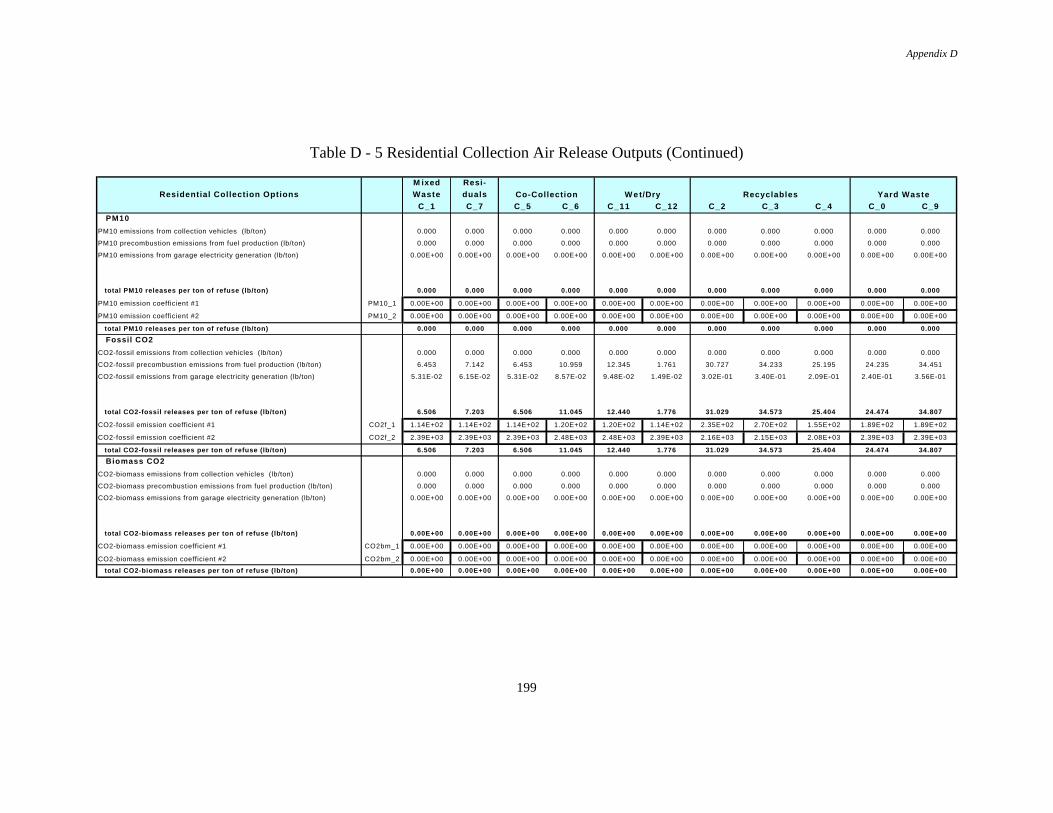
Appendix D
199
Table D - 5 Residential Collection Air Release Outputs (Continued)
M ixed Resi-
Residential Collection Options Waste duals
C_1 C_7 C_5 C_6 C_11 C_12 C_2 C_3 C_4 C_0 C_9
PM10
PM10 emissions from collection vehicles (lb/ton) 0.000 0.000 0.000 0.000 0.000 0.000 0.000 0.000 0.000 0.000 0.000
PM10 precombustion emissions from fuel production (lb/ton) 0.000 0.000 0.000 0.000 0.000 0.000 0.000 0.000 0.000 0.000 0.000
PM10 emissions from garage electricity generation (lb/ton) 0.00E+00 0.00E+00 0.00E+00 0.00E+00 0.00E+00 0.00E+00 0.00E+00 0.00E+00 0.00E+00 0.00E+00 0.00E+00
total PM10 releases per ton of refuse (lb/ton) 0.000 0.000 0.000 0.000 0.000 0.000 0.000 0.000 0.000 0.000 0.000
PM10 emission coefficient #1 PM10_1 0.00E+00 0.00E+00 0.00E+00 0.00E+00 0.00E+00 0.00E+00 0.00E+00 0.00E+00 0.00E+00 0.00E+00 0.00E+00
PM10 emission coefficient #2 PM10_2 0.00E+00 0.00E+00 0.00E+00 0.00E+00 0.00E+00 0.00E+00 0.00E+00 0.00E+00 0.00E+00 0.00E+00 0.00E+00
total PM10 releases per ton of refuse (lb/ton) 0.000 0.000 0.000 0.000 0.000 0.000 0.000 0.000 0.000 0.000 0.000
Fossil CO2
CO2-fossil emissions from collection vehicles (lb/ton) 0.000 0.000 0.000 0.000 0.000 0.000 0.000 0.000 0.000 0.000 0.000
CO2-fossil precombustion emissions from fuel production (lb/ton) 6.453 7.142 6.453 10.959 12.345 1.761 30.727 34.233 25.195 24.235 34.451
CO2-fossil emissions from garage electricity generation (lb/ton) 5.31E-02 6.15E-02 5.31E-02 8.57E-02 9.48E-02 1.49E-02 3.02E-01 3.40E-01 2.09E-01 2.40E-01 3.56E-01
total CO2-fossil releases per ton of refuse (lb/ton) 6.506 7.203 6.506 11.045 12.440 1.776 31.029 34.573 25.404 24.474 34.807
CO2-fossil emission coefficient #1 CO2f_1 1.14E+02 1.14E+02 1.14E+02 1.20E+02 1.20E+02 1.14E+02 2.35E+02 2.70E+02 1.55E+02 1.89E+02 1.89E+02
CO2-fossil emission coefficient #2 CO2f_2 2.39E+03 2.39E+03 2.39E+03 2.48E+03 2.48E+03 2.39E+03 2.16E+03 2.15E+03 2.08E+03 2.39E+03 2.39E+03
total CO2-fossil releases per ton of refuse (lb/ton) 6.506 7.203 6.506 11.045 12.440 1.776 31.029 34.573 25.404 24.474 34.807
Biomass CO2
CO2-biomass emissions from collection vehicles (lb/ton) 0.000 0.000 0.000 0.000 0.000 0.000 0.000 0.000 0.000 0.000 0.000
CO2-biomass precombustion emissions from fuel production (lb/ton) 0.000 0.000 0.000 0.000 0.000 0.000 0.000 0.000 0.000 0.000 0.000
CO2-biomass emissions from garage electricity generation (lb/ton) 0.00E+00 0.00E+00 0.00E+00 0.00E+00 0.00E+00 0.00E+00 0.00E+00 0.00E+00 0.00E+00 0.00E+00 0.00E+00
total CO2-biomass releases per ton of refuse (lb/ton) 0.00E+00 0.00E+00 0.00E+00 0.00E+00 0.00E+00 0.00E+00 0.00E+00 0.00E+00 0.00E+00 0.00E+00 0.00E+00
CO2-biomass emission coefficient #1 CO2bm_1 0.00E+00 0.00E+00 0.00E+00 0.00E+00 0.00E+00 0.00E+00 0.00E+00 0.00E+00 0.00E+00 0.00E+00 0.00E+00
CO2-biomass emission coefficient #2 CO2bm_2 0.00E+00 0.00E+00 0.00E+00 0.00E+00 0.00E+00 0.00E+00 0.00E+00 0.00E+00 0.00E+00 0.00E+00 0.00E+00
total CO2-biomass releases per ton of refuse (lb/ton) 0.00E+00 0.00E+00 0.00E+00 0.00E+00 0.00E+00 0.00E+00 0.00E+00 0.00E+00 0.00E+00 0.00E+00 0.00E+00
Co-Collection W e t/Dry Recyclables Yard Waste
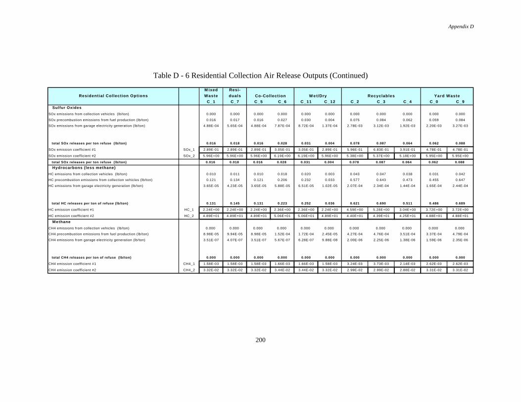
Appendix D
200
Table D - 6 Residential Collection Air Release Outputs (Continued)
M ixed Resi-
Residential Collection Options Waste duals
C_1 C_7 C_5 C_6 C_11 C_12 C_2 C_3 C_4 C_0 C_9
Sulfur Oxides
SOx emissions from collection vehicles (lb/ton) 0.000 0.000 0.000 0.000 0.000 0.000 0.000 0.000 0.000 0.000 0.000
SOx precombustion emissions from fuel production (lb/ton) 0.016 0.017 0.016 0.027 0.030 0.004 0.075 0.084 0.062 0.059 0.084
SOx emissions from garage electricity generation (lb/ton) 4.88E-04 5.65E-04 4.88E-04 7.87E-04 8.72E-04 1.37E-04 2.78E-03 3.12E-03 1.92E-03 2.20E-03 3.27E-03
total SOx releases per ton refuse (lb/ton) 0.016 0.018 0.016 0.028 0.031 0.004 0.078 0.087 0.064 0.062 0.088
SOx emission coefficient #1 SOx_1 2.89E-01 2.89E-01 2.89E-01 3.05E-01 3.05E-01 2.89E-01 5.96E-01 6.83E-01 3.91E-01 4.78E-01 4.78E-01
SOx emission coefficient #2 SOx_2 5.96E+00 5.96E+00 5.96E+00 6.19E+00 6.19E+00 5.96E+00 5.38E+00 5.37E+00 5.18E+00 5.95E+00 5.95E+00
total SOx releases per ton refuse (lb/ton) 0.016 0.018 0.016 0.028 0.031 0.004 0.078 0.087 0.064 0.062 0.088
Hydrocarbons (less methane)
HC emissions from collection vehicles (lb/ton) 0.010 0.011 0.010 0.018 0.020 0.003 0.043 0.047 0.038 0.031 0.042
HC precombustion emissions from collection vehicles (lb/ton) 0.121 0.134 0.121 0.206 0.232 0.033 0.577 0.643 0.473 0.455 0.647
HC emissions from garage electricity generation (lb/ton) 3.65E-05 4.23E-05 3.65E-05 5.88E-05 6.51E-05 1.02E-05 2.07E-04 2.34E-04 1.44E-04 1.65E-04 2.44E-04
total HC releases per ton of refuse (lb/ton) 0.131 0.145 0.131 0.223 0.252 0.036 0.621 0.690 0.511 0.486 0.689
HC emission coefficient #1 HC_1 2.24E+00 2.24E+00 2.24E+00 2.36E+00 2.36E+00 2.24E+00 4.59E+00 5.28E+00 3.04E+00 3.72E+00 3.72E+00
HC emission coefficient #2 HC_2 4.89E+01 4.89E+01 4.89E+01 5.06E+01 5.06E+01 4.89E+01 4.40E+01 4.39E+01 4.25E+01 4.88E+01 4.88E+01
Methane
CH4 emissions from collection vehicles (lb/ton) 0.000 0.000 0.000 0.000 0.000 0.000 0.000 0.000 0.000 0.000 0.000
CH4 precombustion emissions from fuel production (lb/ton) 8.98E-05 9.94E-05 8.98E-05 1.52E-04 1.72E-04 2.45E-05 4.27E-04 4.76E-04 3.51E-04 3.37E-04 4.79E-04
CH4 emissions from garage electricity generation (lb/ton) 3.51E-07 4.07E-07 3.51E-07 5.67E-07 6.28E-07 9.88E-08 2.00E-06 2.25E-06 1.38E-06 1.59E-06 2.35E-06
total CH4 releases per ton of refuse (lb/ton) 0.000 0.000 0.000 0.000 0.000 0.000 0.000 0.000 0.000 0.000 0.000
CH4 emission coefficient #1 CH4_1 1.58E-03 1.58E-03 1.58E-03 1.66E-03 1.66E-03 1.58E-03 3.24E-03 3.73E-03 2.14E-03 2.62E-03 2.62E-03
CH4 emission coefficient #2 CH4_2 3.32E-02 3.32E-02 3.32E-02 3.44E-02 3.44E-02 3.32E-02 2.99E-02 2.99E-02 2.88E-02 3.31E-02 3.31E-02
Co-Collection W e t/Dry Recyclables Yard Waste
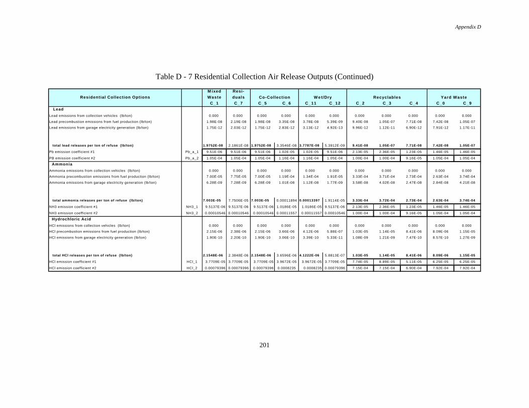
Appendix D
201
Table D - 7 Residential Collection Air Release Outputs (Continued)
M ixed Resi-
Residential Collection Options Waste duals
C_1 C_7 C_5 C_6 C_11 C_12 C_2 C_3 C_4 C_0 C_9
Lead
Lead emissions from collection vehicles (lb/ton) 0.000 0.000 0.000 0.000 0.000 0.000 0.000 0.000 0.000 0.000 0.000
Lead precombustion emissions from fuel production (lb/ton) 1.98E-08 2.19E-08 1.98E-08 3.35E-08 3.78E-08 5.39E-09 9.40E-08 1.05E-07 7.71E-08 7.42E-08 1.05E-07
Lead emissions from garage electricity generation (lb/ton) 1.75E-12 2.03E-12 1.75E-12 2.83E-12 3.13E-12 4.92E-13 9.96E-12 1.12E-11 6.90E-12 7.91E-12 1.17E-11
total lead releases per ton of refuse (lb/ton) 1.9752E-08 2.1861E-08 1.9752E-08 3.3546E-08 3.7787E-08 5.3912E-09 9.41E-08 1.05E-07 7.71E-08 7.42E-08 1.05E-07
Pb emission coefficient #1 Pb_a_1 9.51E-06 9.51E-06 9.51E-06 1.02E-05 1.02E-05 9.51E-06 2.13E-05 2.36E-05 1.23E-05 1.46E-05 1.46E-05
PB emission coefficient #2 Pb_a_2 1.05E-04 1.05E-04 1.05E-04 1.16E-04 1.16E-04 1.05E-04 1.00E-04 1.00E-04 9.16E-05 1.05E-04 1.05E-04
Ammonia
Ammonia emissions from collection vehicles (lb/ton) 0.000 0.000 0.000 0.000 0.000 0.000 0.000 0.000 0.000 0.000 0.000
Ammonia precombustion emissions from fuel production (lb/ton) 7.00E-05 7.75E-05 7.00E-05 1.19E-04 1.34E-04 1.91E-05 3.33E-04 3.71E-04 2.73E-04 2.63E-04 3.74E-04
Ammonia emissions from garage electricity generation (lb/ton) 6.28E-09 7.28E-09 6.28E-09 1.01E-08 1.12E-08 1.77E-09 3.58E-08 4.02E-08 2.47E-08 2.84E-08 4.21E-08
total ammonia releases per ton of refuse (lb/ton) 7.003E-05 7.7506E-05 7.003E-05 0.00011894 0.00013397 1.9114E-05 3.33E-04 3.72E-04 2.73E-04 2.63E-04 3.74E-04
NH3 emission coefficient #1 NH3_1 9.5137E-06 9.5137E-06 9.5137E-06 1.0186E-05 1.0186E-05 9.5137E-06 2.13E-05 2.36E-05 1.23E-05 1.46E-05 1.46E-05
NH3 emission coefficient #2 NH3_2 0.00010546 0.00010546 0.00010546 0.00011557 0.00011557 0.00010546 1.00E-04 1.00E-04 9.16E-05 1.05E-04 1.05E-04
Hydrochloric Acid
HCl emissions from collection vehicles (lb/ton) 0.000 0.000 0.000 0.000 0.000 0.000 0.000 0.000 0.000 0.000 0.000
HCl precombustion emissions from fuel production (lb/ton) 2.15E-06 2.38E-06 2.15E-06 3.66E-06 4.12E-06 5.88E-07 1.03E-05 1.14E-05 8.41E-06 8.09E-06 1.15E-05
HCl emissions from garage electricity generation (lb/ton) 1.90E-10 2.20E-10 1.90E-10 3.06E-10 3.39E-10 5.33E-11 1.08E-09 1.21E-09 7.47E-10 8.57E-10 1.27E-09
total HCl releases per ton of refuse (lb/ton) 2.1548E-06 2.3848E-06 2.1548E-06 3.6596E-06 4.1222E-06 5.8813E-07 1.03E-05 1.14E-05 8.41E-06 8.09E-06 1.15E-05
HCl emission coefficient #1 HCl_1 3.7709E-05 3.7709E-05 3.7709E-05 3.9672E-05 3.9672E-05 3.7709E-05 7.74E-05 8.89E-05 5.11E-05 6.25E-05 6.25E-05
HCl emission coefficient #2 HCl_2 0.00079396 0.00079396 0.00079396 0.0008235 0.0008235 0.00079396 7.15E-04 7.15E-04 6.90E-04 7.92E-04 7.92E-04
Co-Collection W e t/Dry Recyclables Yard Waste

Appendix D
202
Table D - 8 Residential Collection Air Release Outputs (Continued)
M ixed Resi-
Residential Collection Options Waste duals
C_1 C_7 C_5 C_6 C_11 C_12 C_2 C_3 C_4 C_0 C_9
Greenhouse Gas Equivalence
Carbon dioxide (fossil fuel) 6.51 7.20 6.51 11.05 12.44 1.78 31.03 34.57 25.40 24.47 34.81
Carbon dioxide (biomass) 0.00E+00 0.00 0.00 0.00 0.00 0.00 0.00 0.00 0.00 0.00 0.00
Methane 0.01 0.01 0.01 0.01 0.01 0.00 0.03 0.03 0.02 0.02 0.03
Nitrogen oxides 152.91 164.20 152.91 270.83 308.05 40.95 669.04 729.15 584.41 475.17 644.89
Other hydrocarbons 0.00 0.00 0.00 0.00 0.00 0.00 0.00 0.00 0.00 0.00 0.00
total greenhouse gas equivalence per ton of refuse 159.41898 171.404828 159.41898 281.887854 320.503397 42.7286583 700.10 763.75 609.84 499.67 679.73
GHE emission coefficient #1 GHE_1 1964.99802 1964.99802 1964.99802 2060.90254 2060.90254 1964.99802 3.97E+03 4.59E+03 2.68E+03 3.30E+03 3.30E+03
GHE emission coefficient #2 GHE_2 67296.9497 67296.9497 67296.9497 68740.3959 68740.3959 67296.9497 5.97E+04 5.97E+04 5.85E+04 6.72E+04 6.72E+04
Co-Collection W e t/Dry Recyclables Yard Waste

Appendix D
203
Table D - 9 Residential Collection Water Release Outputs (Continued)
M ixed Resi-
Residential Collection Options Waste duals
C_1 C_7 C_5 C_6 C_11 C_12 C_2 C_3 C_4 C_0 C_9
WATERBORNE RELEASES
D issolved Solids
Dissolved solids emissions from washdown water (lb/ton) 0.00E+00 0.00E+00 0.00E+00 0.00E+00 0.00E+00 0.00E+00 0.00E+00 0.00E+00 0.00E+00 0.00E+00 0.00E+00
DS precombustion emissions from fuel production (lb/ton) 1.83E-01 2.03E-01 1.83E-01 3.11E-01 3.50E-01 5.00E-02 8.72E-01 9.72E-01 7.15E-01 6.88E-01 9.78E-01
DS emissions from garage electricity generation (lb/ton) 1.63E-05 1.89E-05 1.63E-05 2.63E-05 2.91E-05 4.58E-06 9.28E-05 1.04E-04 6.42E-05 7.37E-05 1.09E-04
total dissolved solids releases per ton of refuse (lb/ton) 0.1831557 0.20270685 0.1831557 0.31106258 0.35038435 0.04999078 8.72E-01 9.72E-01 7.15E-01 6.88E-01 9.78E-01
DS emission coefficient #1 DS_1 3.20527668 3.20527668 3.20527668 3.37212246 3.37212246 3.20527668 6.57646669 7.55472572 4.341004862 5.314486163 5.314486163
DS emission coefficient #2 DS_2 67.4863809 67.4863809 67.4863809 69.9975546 69.9975546 67.4863809 60.80541147 60.75224522 58.62208513 67.35455532 67.35455532
DS emission coefficient #3 DS_3 0.00E+00 0.00E+00 0.00E+00 0.00E+00 0.00E+00 0.00E+00 0.00E+00 0.00E+00 0.00E+00 0.00E+00 0.00E+00
Suspended Solids
Suspended solids emissions from washdown water (lb/ton) 0.00E+00 0.00E+00 0.00E+00 0.00E+00 0.00E+00 0.00E+00 0.00E+00 0.00E+00 0.00E+00 0.00E+00 0.00E+00
SS precombustion emissions from fuel production (lb/ton) 1.71E-04 1.89E-04 1.71E-04 2.90E-04 3.26E-04 4.66E-05 8.12E-04 9.05E-04 6.66E-04 6.41E-04 9.11E-04
SS emissions from garage electricity generation (lb/ton) 1.47E-08 1.70E-08 1.47E-08 2.37E-08 2.62E-08 4.13E-09 8.36E-08 9.41E-08 5.78E-08 6.64E-08 9.84E-08
total suspended solids releases per ton of refuse (lb/ton) 0.00017059 0.0001888 0.00017059 0.00028971 0.00032634 4.656E-05 8.12E-04 9.05E-04 6.66E-04 6.41E-04 9.11E-04
SS emission coefficient #1 SS_1 0.00298529 0.00298529 0.00298529 0.00314069 0.00314069 0.00298529 0.006125111 0.007036231 0.004043076 0.004949746 0.004949746
SS emission coefficient #2 SS_2 0.06285482 0.06285482 0.06285482 0.06519365 0.06519365 0.06285482 0.056632356 0.056582839 0.054598878 0.062732043 0.062732043
SS emission coefficient #3 SS_3 0.00E+00 0.00E+00 0.00E+00 0.00E+00 0.00E+00 0.00E+00 0.00E+00 0.00E+00 0.00E+00 0.00E+00 0.00E+00
Biochemical Oxygen Demand
BOD emissions from washdown water (lb/ton) 0.00E+00 0.00E+00 0.00E+00 0.00E+00 0.00E+00 0.00E+00 0.00E+00 0.00E+00 0.00E+00 0.00E+00 0.00E+00
BOD precombustion emissions from fuel production (lb/ton) 1.80E-04 1.99E-04 1.80E-04 3.05E-04 3.43E-04 4.90E-05 8.55E-04 9.52E-04 7.01E-04 6.74E-04 9.59E-04
BOD emissions from garage electricity generation (lb/ton) 1.61E-08 1.87E-08 1.61E-08 2.60E-08 2.87E-08 4.52E-09 9.16E-08 1.03E-07 6.34E-08 7.27E-08 1.08E-07
total BOD releases per ton of refuse (lb/ton) 0.00017956 0.00019873 0.00017956 0.00030496 0.00034351 4.9011E-05 8.55E-04 9.53E-04 7.01E-04 6.74E-04 9.59E-04
BOD emission coefficient #1 BOD_1 0.00314243 0.00314243 0.00314243 0.00330601 0.00330601 0.00314243 0.006447522 0.007406601 0.004255891 0.005210285 0.005210285
BOD emission coefficient #2 BOD_2 0.06616315 0.06616315 0.06616315 0.06862509 0.06862509 0.06616315 0.059613176 0.059561052 0.057472658 0.066033907 0.066033907
BOD emission coefficient #3 BOD_3 0.00E+00 0.00E+00 0.00E+00 0.00E+00 0.00E+00 0.00E+00 0.00E+00 0.00E+00 0.00E+00 0.00E+00 0.00E+00
Co-Collection W e t/Dry Recyclables Yard Waste
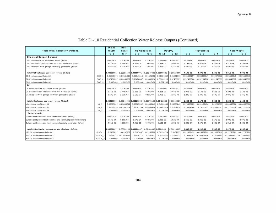
Appendix D
204
Table D - 10 Residential Collection Water Release Outputs (Continued)
M ixed Resi-
Residential Collection Options Waste duals
C_1 C_7 C_5 C_6 C_11 C_12 C_2 C_3 C_4 C_0 C_9
Chemical Oxygen Demand
COD emissions from washdown water (lb/ton) 0.00E+00 0.00E+00 0.00E+00 0.00E+00 0.00E+00 0.00E+00 0.00E+00 0.00E+00 0.00E+00 0.00E+00 0.00E+00
COD precombustion emissions from fuel production (lb/ton) 8.81E-04 9.75E-04 8.81E-04 1.50E-03 1.69E-03 2.40E-04 4.19E-03 4.67E-03 3.44E-03 3.31E-03 4.70E-03
COD emissions from garage electricity generation (lb/ton) 7.96E-08 9.23E-08 7.96E-08 1.29E-07 1.42E-07 2.24E-08 4.53E-07 5.10E-07 3.14E-07 3.60E-07 5.34E-07
total COD releases per ton of refuse (lb/ton) 0.00088091 0.00097494 0.00088091 0.00149609 0.00168521 0.00024044 4.19E-03 4.67E-03 3.44E-03 3.31E-03 4.70E-03
COD emission coefficient #1 COD_1 0.01541616 0.01541616 0.01541616 0.01621862 0.01621862 0.01541616 0.031630297 0.036335347 0.020878572 0.025560643 0.025560643
COD emission coefficient #2 COD_2 0.32458337 0.32458337 0.32458337 0.33666116 0.33666116 0.32458337 0.292450508 0.292194798 0.281949535 0.323949335 0.323949335
COD emission coefficient #3 COD_3 0.00E+00 0.00E+00 0.00E+00 0.00E+00 0.00E+00 0.00E+00 0.00E+00 0.00E+00 0.00E+00 0.00E+00 0.00E+00
Oil
Oil emissions from washdown water (lb/ton) 0.00E+00 0.00E+00 0.00E+00 0.00E+00 0.00E+00 0.00E+00 0.00E+00 0.00E+00 0.00E+00 0.00E+00 0.00E+00
Oil precombustion emissions from fuel production (lb/ton) 2.21E-03 2.44E-03 2.21E-03 3.75E-03 4.22E-03 6.03E-04 1.05E-02 1.17E-02 8.62E-03 8.29E-03 1.18E-02
Oil emissions from garage electricity generation (lb/ton) 2.18E-07 2.53E-07 2.18E-07 3.52E-07 3.90E-07 6.13E-08 1.24E-06 1.40E-06 8.59E-07 9.86E-07 1.46E-06
total oil releases per ton of refuse (lb/ton) 0.00220866 0.00244443 0.00220866 0.00375108 0.00422526 0.00060284 1.05E-02 1.17E-02 8.62E-03 8.29E-03 1.18E-02
oil emission coefficient #1 oil_1 0.03865242 0.03865242 0.03865242 0.04066443 0.04066443 0.03865242 0.079305703 0.091102494 0.05234813 0.064087306 0.064087306
oil emission coefficient #2 oil_2 0.81381234 0.81381234 0.81381234 0.84409474 0.84409474 0.81381234 0.73324744 0.73260631 0.706918571 0.812222658 0.812222658
oil emission coefficient #3 oil_3 0.00E+00 0.00E+00 0.00E+00 0.00E+00 0.00E+00 0.00E+00 0.00E+00 0.00E+00 0.00E+00 0.00E+00 0.00E+00
Sulfuric Acid
Sulfuric acid emissions from washdown water (lb/ton) 0.00E+00 0.00E+00 0.00E+00 0.00E+00 0.00E+00 0.00E+00 0.00E+00 0.00E+00 0.00E+00 0.00E+00 0.00E+00
Sulfuric acid precombustion emissions from fuel production (lb/ton) 5.57E-04 6.16E-04 5.57E-04 9.45E-04 1.06E-03 1.52E-04 2.65E-03 2.95E-03 2.17E-03 2.09E-03 2.97E-03
Sulfuric acid emissions from garage electricity generation (lb/ton) 4.01E-05 4.65E-05 4.01E-05 6.47E-05 7.16E-05 1.13E-05 2.28E-04 2.57E-04 1.58E-04 1.81E-04 2.68E-04
total sulfuric acid releases per ton of refuse (lb/ton) 0.00059667 0.00066246 0.00059667 0.00100998 0.0011364 0.00016318 2.88E-03 3.21E-03 2.33E-03 2.27E-03 3.24E-03
H2SO4 emission coefficient #1 H2SO4_1 0.0107857 0.0107857 0.0107857 0.01136729 0.01136729 0.0107857 0.022328432 0.025559729 0.014536119 0.017750762 0.017750762
H2SO4 emission coefficient #2 H2SO4_2 0.21628772 0.21628772 0.21628772 0.2250411 0.2250411 0.21628772 0.19548303 0.195307416 0.18787245 0.215852402 0.215852402
H2SO4 emission coefficient #3 H2SO4_3 0.00E+00 0.00E+00 0.00E+00 0.00E+00 0.00E+00 0.00E+00 0.00E+00 0.00E+00 0.00E+00 0.00E+00 0.00E+00
Co-Collection W e t/Dry Recyclables Yard Waste

Appendix D
205
Table D - 11 Residential Collection Water Release Outputs (Continued)
M ixed Resi-
Residential Collection Options Waste duals
C_1 C_7 C_5 C_6 C_11 C_12 C_2 C_3 C_4 C_0 C_9
Iron
Iron emissions from washdown water (lb/ton) 0.00E+00 0.00E+00 0.00E+00 0.00E+00 0.00E+00 0.00E+00 0.00E+00 0.00E+00 0.00E+00 0.00E+00 0.00E+00
Iron precombustion emissions from fuel production (lb/ton) 1.45E-04 1.61E-04 1.45E-04 2.47E-04 2.78E-04 3.97E-05 6.93E-04 7.72E-04 5.68E-04 5.46E-04 7.76E-04
Iron emissions from garage electricity generation (lb/ton) 9.97E-06 1.16E-05 9.97E-06 1.61E-05 1.78E-05 2.80E-06 5.67E-05 6.39E-05 3.93E-05 4.51E-05 6.68E-05
total iron releases per ton of refuse (lb/ton) 0.0001554 0.00017251 0.0001554 0.00026309 0.00029603 4.2497E-05 7.49E-04 8.35E-04 6.07E-04 5.91E-04 8.43E-04
fe emission coefficient #1 fe_1 0.00280511 0.00280511 0.00280511 0.00295614 0.00295614 0.00280511 0.005804851 0.006645921 0.003781311 0.004618056 0.004618056
fe emission coefficient #2 fe_2 0.05637369 0.05637369 0.05637369 0.05864681 0.05864681 0.05637369 0.050943893 0.050898183 0.048967546 0.056260382 0.056260382
fe emission coefficient #3 fe_3 0.00E+00 0.00E+00 0.00E+00 0.00E+00 0.00E+00 0.00E+00 0.00E+00 0.00E+00 0.00E+00 0.00E+00 0.00E+00
Ammonia
Ammonia emissions from washdown water (lb/ton) 0.00E+00 0.00E+00 0.00E+00 0.00E+00 0.00E+00 0.00E+00 0.00E+00 0.00E+00 0.00E+00 0.00E+00 0.00E+00
Ammonia precombustion emissions from fuel production (lb/ton) 2.51E-05 2.78E-05 2.51E-05 4.27E-05 4.81E-05 6.86E-06 1.20E-04 1.33E-04 9.81E-05 9.44E-05 1.34E-04
Ammonia emissions from garage electricity generation (lb/ton) 2.19E-09 2.54E-09 2.19E-09 3.54E-09 3.92E-09 6.17E-10 1.25E-08 1.41E-08 8.64E-09 9.92E-09 1.47E-08
total ammonia releases per ton of refuse (lb/ton) 2.5139E-05 2.7822E-05 2.5139E-05 4.2695E-05 4.8092E-05 6.8615E-06 1.20E-04 1.33E-04 9.82E-05 9.44E-05 1.34E-04
NH4 emission coefficient #1 NH4_1 0.00043994 0.00043994 0.00043994 0.00046284 0.00046284 0.00043994 0.00090265 0.00103692 0.000595823 0.000729437 0.000729437
NH4 emission coefficient #2 NH4_2 0.00926282 0.00926282 0.00926282 0.00960749 0.00960749 0.00926282 0.008345829 0.008338532 0.008046158 0.00924473 0.00924473
NH4 emission coefficient #3 NH4_3 0.00E+00 0.00E+00 0.00E+00 0.00E+00 0.00E+00 0.00E+00 0.00E+00 0.00E+00 0.00E+00 0.00E+00 0.00E+00
Copper
Copper emissions from washdown water (lb/ton) 0.00E+00 0.00E+00 0.00E+00 0.00E+00 0.00E+00 0.00E+00 0.00E+00 0.00E+00 0.00E+00 0.00E+00 0.00E+00
Copper precombustion emissions from fuel production (lb/ton) 0.00E+00 0.00E+00 0.00E+00 0.00E+00 0.00E+00 0.00E+00 0.00E+00 0.00E+00 0.00E+00 0.00E+00 0.00E+00
Copper emissions from garage electricity generation (lb/ton) 0.00E+00 0.00E+00 0.00E+00 0.00E+00 0.00E+00 0.00E+00 0.00E+00 0.00E+00 0.00E+00 0.00E+00 0.00E+00
total copper releases per ton of refuse (lb/ton) 0 0 0 0 0 0 0.00E+00 0.00E+00 0.00E+00 0.00E+00 0.00E+00
cu emission coefficient #1 cu_1 0 0 0 0 0 0 0 0 0 0 0
cu emission coefficient #2 cu_2 0 0 0 0 0 0 0 0 0 0 0
cu emission coefficient #3 cu_3 0.00E+00 0.00E+00 0.00E+00 0.00E+00 0.00E+00 0.00E+00 0.00E+00 0.00E+00 0.00E+00 0.00E+00 0.00E+00
Co-Collection W e t/Dry Recyclables Yard Waste

Appendix D
206
Table D - 12 Residential Collection Water Release Outputs (Continued)
M ixed Resi-
Residential Collection Options Waste duals
C_1 C_7 C_5 C_6 C_11 C_12 C_2 C_3 C_4 C_0 C_9
Cadmium
Cadmium emissions from washdown water (lb/ton) 0.00E+00 0.00E+00 0.00E+00 0.00E+00 0.00E+00 0.00E+00 0.00E+00 0.00E+00 0.00E+00 0.00E+00 0.00E+00
Cadmium precombustion emissions from fuel production (lb/ton) 0.00E+00 0.00E+00 0.00E+00 0.00E+00 0.00E+00 0.00E+00 0.00E+00 0.00E+00 0.00E+00 0.00E+00 0.00E+00
Cadmium emissions from garage electricity generation (lb/ton) 0.00E+00 0.00E+00 0.00E+00 0.00E+00 0.00E+00 0.00E+00 0.00E+00 0.00E+00 0.00E+00 0.00E+00 0.00E+00
total cadmium releases per ton of refuse (lb/ton) 0 0 0 0 0 0 0.00E+00 0.00E+00 0.00E+00 0.00E+00 0.00E+00
cd emission coefficient #1 cd_1 0 0 0 0 0 0 0 0 0 0 0
cd emission coefficient #2 cd_2 0 0 0 0 0 0 0 0 0 0 0
cd emission coefficient #3 cd_3 0.00E+00 0.00E+00 0.00E+00 0.00E+00 0.00E+00 0.00E+00 0.00E+00 0.00E+00 0.00E+00 0.00E+00 0.00E+00
Arsenic
Arsenic emissions from washdown water (lb/ton) 0.00E+00 0.00E+00 0.00E+00 0.00E+00 0.00E+00 0.00E+00 0.00E+00 0.00E+00 0.00E+00 0.00E+00 0.00E+00
Arsenic precombustion emissions from fuel production (lb/ton) 0.00E+00 0.00E+00 0.00E+00 0.00E+00 0.00E+00 0.00E+00 0.00E+00 0.00E+00 0.00E+00 0.00E+00 0.00E+00
Arsenic emissions from garage electricity generation (lb/ton) 0.00E+00 0.00E+00 0.00E+00 0.00E+00 0.00E+00 0.00E+00 0.00E+00 0.00E+00 0.00E+00 0.00E+00 0.00E+00
total arsenic releases per ton of refuse (lb/ton) 0 0 0 0 0 0 0.00E+00 0.00E+00 0.00E+00 0.00E+00 0.00E+00
as emission coefficient #1 as_1 0 0 0 0 0 0 0 0 0 0 0
as emission coefficient #2 as_2 0 0 0 0 0 0 0 0 0 0 0
as emission coefficient #3 as_3 0.00E+00 0.00E+00 0.00E+00 0.00E+00 0.00E+00 0.00E+00 0.00E+00 0.00E+00 0.00E+00 0.00E+00 0.00E+00
Mercury
Mercury emissions from washdown water (lb/ton) 0.00E+00 0.00E+00 0.00E+00 0.00E+00 0.00E+00 0.00E+00 0.00E+00 0.00E+00 0.00E+00 0.00E+00 0.00E+00
Mercury precombustion emissions from fuel production (lb/ton) 0.00E+00 0.00E+00 0.00E+00 0.00E+00 0.00E+00 0.00E+00 0.00E+00 0.00E+00 0.00E+00 0.00E+00 0.00E+00
Mercury emissions from garage electricity generation (lb/ton) 0.00E+00 0.00E+00 0.00E+00 0.00E+00 0.00E+00 0.00E+00 0.00E+00 0.00E+00 0.00E+00 0.00E+00 0.00E+00
total mercury releases per ton of refuse (lb/ton) 0 0 0 0 0 0 0.00E+00 0.00E+00 0.00E+00 0.00E+00 0.00E+00
hg emission coefficient #1 hg_1 0 0 0 0 0 0 0 0 0 0 0
hg emission coefficient #2 hg_2 0 0 0 0 0 0 0 0 0 0 0
hg emission coefficient #3 hg_3 0.00E+00 0.00E+00 0.00E+00 0.00E+00 0.00E+00 0.00E+00 0.00E+00 0.00E+00 0.00E+00 0.00E+00 0.00E+00
Co-Collection W e t/Dry Recyclables Yard Waste
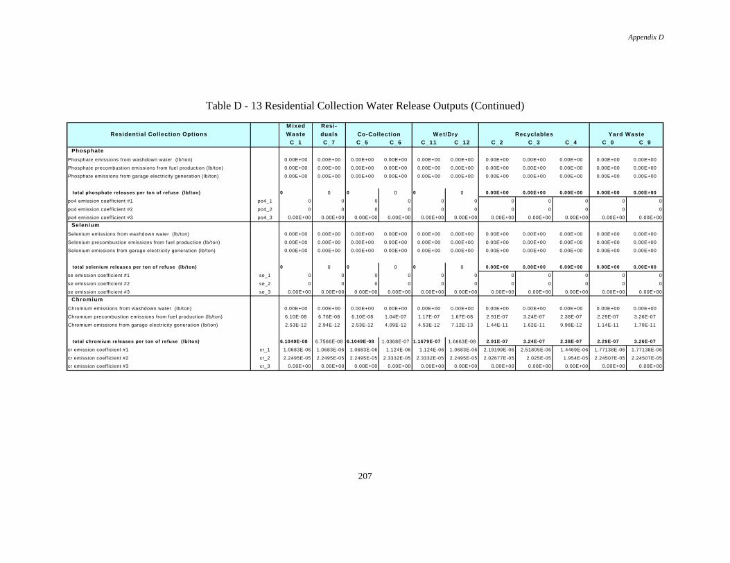
Appendix D
207
Table D - 13 Residential Collection Water Release Outputs (Continued)
M ixed Resi-
Residential Collection Options Waste duals
C_1 C_7 C_5 C_6 C_11 C_12 C_2 C_3 C_4 C_0 C_9
Phosphate
Phosphate emissions from washdown water (lb/ton) 0.00E+00 0.00E+00 0.00E+00 0.00E+00 0.00E+00 0.00E+00 0.00E+00 0.00E+00 0.00E+00 0.00E+00 0.00E+00
Phosphate precombustion emissions from fuel production (lb/ton) 0.00E+00 0.00E+00 0.00E+00 0.00E+00 0.00E+00 0.00E+00 0.00E+00 0.00E+00 0.00E+00 0.00E+00 0.00E+00
Phosphate emissions from garage electricity generation (lb/ton) 0.00E+00 0.00E+00 0.00E+00 0.00E+00 0.00E+00 0.00E+00 0.00E+00 0.00E+00 0.00E+00 0.00E+00 0.00E+00
total phosphate releases per ton of refuse (lb/ton) 0 0 0 0 0 0 0.00E+00 0.00E+00 0.00E+00 0.00E+00 0.00E+00
po4 emission coefficient #1 po4_1 0 0 0 0 0 0 0 0 0 0 0
po4 emission coefficient #2 po4_2 0 0 0 0 0 0 0 0 0 0 0
po4 emission coefficient #3 po4_3 0.00E+00 0.00E+00 0.00E+00 0.00E+00 0.00E+00 0.00E+00 0.00E+00 0.00E+00 0.00E+00 0.00E+00 0.00E+00
Selenium
Selenium emissions from washdown water (lb/ton) 0.00E+00 0.00E+00 0.00E+00 0.00E+00 0.00E+00 0.00E+00 0.00E+00 0.00E+00 0.00E+00 0.00E+00 0.00E+00
Selenium precombustion emissions from fuel production (lb/ton) 0.00E+00 0.00E+00 0.00E+00 0.00E+00 0.00E+00 0.00E+00 0.00E+00 0.00E+00 0.00E+00 0.00E+00 0.00E+00
Selenium emissions from garage electricity generation (lb/ton) 0.00E+00 0.00E+00 0.00E+00 0.00E+00 0.00E+00 0.00E+00 0.00E+00 0.00E+00 0.00E+00 0.00E+00 0.00E+00
total selenium releases per ton of refuse (lb/ton) 0 0 0 0 0 0 0.00E+00 0.00E+00 0.00E+00 0.00E+00 0.00E+00
se emission coefficient #1 se_1 0 0 0 0 0 0 0 0 0 0 0
se emission coefficient #2 se_2 0 0 0 0 0 0 0 0 0 0 0
se emission coefficient #3 se_3 0.00E+00 0.00E+00 0.00E+00 0.00E+00 0.00E+00 0.00E+00 0.00E+00 0.00E+00 0.00E+00 0.00E+00 0.00E+00
Chromium
Chromium emissions from washdown water (lb/ton) 0.00E+00 0.00E+00 0.00E+00 0.00E+00 0.00E+00 0.00E+00 0.00E+00 0.00E+00 0.00E+00 0.00E+00 0.00E+00
Chromium precombustion emissions from fuel production (lb/ton) 6.10E-08 6.76E-08 6.10E-08 1.04E-07 1.17E-07 1.67E-08 2.91E-07 3.24E-07 2.38E-07 2.29E-07 3.26E-07
Chromium emissions from garage electricity generation (lb/ton) 2.53E-12 2.94E-12 2.53E-12 4.09E-12 4.53E-12 7.12E-13 1.44E-11 1.62E-11 9.98E-12 1.14E-11 1.70E-11
total chromium releases per ton of refuse (lb/ton) 6.1049E-08 6.7566E-08 6.1049E-08 1.0368E-07 1.1679E-07 1.6663E-08 2.91E-07 3.24E-07 2.38E-07 2.29E-07 3.26E-07
cr emission coefficient #1 cr_1 1.0683E-06 1.0683E-06 1.0683E-06 1.124E-06 1.124E-06 1.0683E-06 2.19199E-06 2.51805E-06 1.4469E-06 1.77138E-06 1.77138E-06
cr emission coefficient #2 cr_2 2.2495E-05 2.2495E-05 2.2495E-05 2.3332E-05 2.3332E-05 2.2495E-05 2.02677E-05 2.025E-05 1.954E-05 2.24507E-05 2.24507E-05
cr emission coefficient #3 cr_3 0.00E+00 0.00E+00 0.00E+00 0.00E+00 0.00E+00 0.00E+00 0.00E+00 0.00E+00 0.00E+00 0.00E+00 0.00E+00
Co-Collection W e t/Dry Recyclables Yard Waste
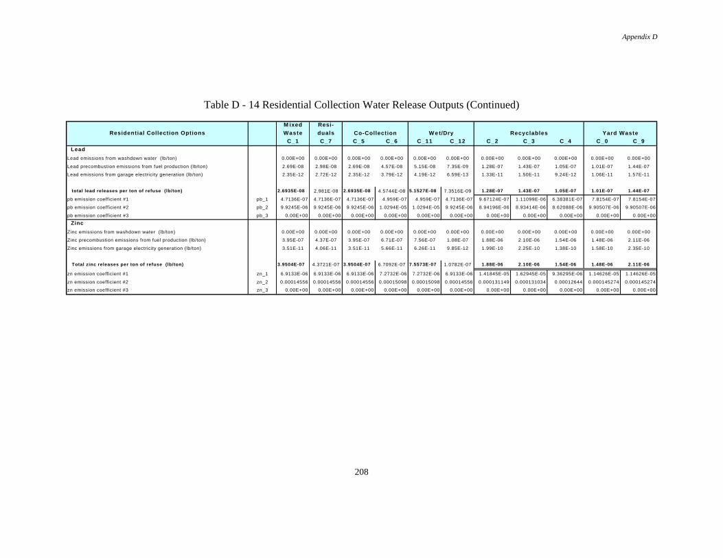
Appendix D
208
Table D - 14 Residential Collection Water Release Outputs (Continued)
M ixed Resi-
Residential Collection Options Waste duals
C_1 C_7 C_5 C_6 C_11 C_12 C_2 C_3 C_4 C_0 C_9
Lead
Lead emissions from washdown water (lb/ton) 0.00E+00 0.00E+00 0.00E+00 0.00E+00 0.00E+00 0.00E+00 0.00E+00 0.00E+00 0.00E+00 0.00E+00 0.00E+00
Lead precombustion emissions from fuel production (lb/ton) 2.69E-08 2.98E-08 2.69E-08 4.57E-08 5.15E-08 7.35E-09 1.28E-07 1.43E-07 1.05E-07 1.01E-07 1.44E-07
Lead emissions from garage electricity generation (lb/ton) 2.35E-12 2.72E-12 2.35E-12 3.79E-12 4.19E-12 6.59E-13 1.33E-11 1.50E-11 9.24E-12 1.06E-11 1.57E-11
total lead releases per ton of refuse (lb/ton) 2.6935E-08 2.981E-08 2.6935E-08 4.5744E-08 5.1527E-08 7.3516E-09 1.28E-07 1.43E-07 1.05E-07 1.01E-07 1.44E-07
pb emission coefficient #1 pb_1 4.7136E-07 4.7136E-07 4.7136E-07 4.959E-07 4.959E-07 4.7136E-07 9.67124E-07 1.11099E-06 6.38381E-07 7.8154E-07 7.8154E-07
pb emission coefficient #2 pb_2 9.9245E-06 9.9245E-06 9.9245E-06 1.0294E-05 1.0294E-05 9.9245E-06 8.94196E-06 8.93414E-06 8.62088E-06 9.90507E-06 9.90507E-06
pb emission coefficient #3 pb_3 0.00E+00 0.00E+00 0.00E+00 0.00E+00 0.00E+00 0.00E+00 0.00E+00 0.00E+00 0.00E+00 0.00E+00 0.00E+00
Zinc
Zinc emissions from washdown water (lb/ton) 0.00E+00 0.00E+00 0.00E+00 0.00E+00 0.00E+00 0.00E+00 0.00E+00 0.00E+00 0.00E+00 0.00E+00 0.00E+00
Zinc precombustion emissions from fuel production (lb/ton) 3.95E-07 4.37E-07 3.95E-07 6.71E-07 7.56E-07 1.08E-07 1.88E-06 2.10E-06 1.54E-06 1.48E-06 2.11E-06
Zinc emissions from garage electricity generation (lb/ton) 3.51E-11 4.06E-11 3.51E-11 5.66E-11 6.26E-11 9.85E-12 1.99E-10 2.25E-10 1.38E-10 1.58E-10 2.35E-10
Total zinc releases per ton of refuse (lb/ton) 3.9504E-07 4.3721E-07 3.9504E-07 6.7092E-07 7.5573E-07 1.0782E-07 1.88E-06 2.10E-06 1.54E-06 1.48E-06 2.11E-06
zn emission coefficient #1 zn_1 6.9133E-06 6.9133E-06 6.9133E-06 7.2732E-06 7.2732E-06 6.9133E-06 1.41845E-05 1.62945E-05 9.36295E-06 1.14626E-05 1.14626E-05
zn emission coefficient #2 zn_2 0.00014556 0.00014556 0.00014556 0.00015098 0.00015098 0.00014556 0.000131149 0.000131034 0.00012644 0.000145274 0.000145274
zn emission coefficient #3 zn_3 0.00E+00 0.00E+00 0.00E+00 0.00E+00 0.00E+00 0.00E+00 0.00E+00 0.00E+00 0.00E+00 0.00E+00 0.00E+00
Co-Collection W e t/Dry Recyclables Yard Waste

Appendix D
209
Table D - 15 Residential Collection Solid Waste Outputs (Continued)
M ixed Resi-
Residential Collection Options Waste duals
C_1 C_7 C_5 C_6 C_11 C_12 C_2 C_3 C_4 C_0 C_9
SOLID WASTE
Solid Waste #1
SW#1 precombustion emissions from fuel production (lb/ton) 1.48E-01 1.64E-01 1.48E-01 2.51E-01 2.83E-01 4.04E-02 7.04E-01 7.85E-01 5.78E-01 5.56E-01 7.90E-01
SW#1 emissions from garage electricity generation (lb/ton) 6.80E-03 7.88E-03 6.80E-03 1.10E-02 1.22E-02 1.91E-03 3.87E-02 4.36E-02 2.68E-02 3.07E-02 4.56E-02
total SW#1 generation per ton of refuse (lb/ton) 0.15475021 0.17162482 0.15475021 0.26224666 0.29518484 0.04229312 7.43E-01 8.28E-01 6.04E-01 5.86E-01 8.35E-01
SW1 emission coefficient #1 SW1_1 2.76647752 2.76647752 2.76647752 2.91390076 2.91390076 2.76647752 5.71E+00 6.54E+00 3.73E+00 4.56E+00 4.56E+00
SW1 emission coefficient #2 SW1_2 56.4151502 56.4151502 56.4151502 58.6339977 58.6339977 56.4151502 5.09E+01 5.09E+01 4.90E+01 5.63E+01 5.63E+01
Solid Waste #2
SW #2 precombustion emissions from fuel production (lb/ton) 0.00E+00 0.00E+00 0.00E+00 0.00E+00 0.00E+00 0.00E+00 0.00E+00 0.00E+00 0.00E+00 0.00E+00 0.00E+00
SW #2 emissions from garage electricity generation (lb/ton) 0.00E+00 0.00E+00 0.00E+00 0.00E+00 0.00E+00 0.00E+00 0.00E+00 0.00E+00 0.00E+00 0.00E+00 0.00E+00
total SW #2 generation per ton of refuse (lb/ton) 0 0 0 0 0 0 0.00E+00 0.00E+00 0.00E+00 0.00E+00 0.00E+00
SW2 emission coefficient #2 SW2_2 0 0 0 0 0 0 0.00E+00 0.00E+00 0.00E+00 0.00E+00 0.00E+00
Solid Waste #3
SW #3 precombustion emissions from fuel production (lb/ton) 0.00E+00 0.00E+00 0.00E+00 0.00E+00 0.00E+00 0.00E+00 0.00E+00 0.00E+00 0.00E+00 0.00E+00 0.00E+00
SW #3 emissions from garage electricity generation (lb/ton) 0.00E+00 0.00E+00 0.00E+00 0.00E+00 0.00E+00 0.00E+00 0.00E+00 0.00E+00 0.00E+00 0.00E+00 0.00E+00
total SW #3 generation per ton of refuse (lb/ton) 0 0 0 0 0 0 0.00E+00 0.00E+00 0.00E+00 0.00E+00 0.00E+00
SW3 emission coefficient #1 SW3_1 0 0 0 0 0 0 0.00E+00 0.00E+00 0.00E+00 0.00E+00 0.00E+00
SW3 emission coefficient #2 SW3_2 0 0 0 0 0 0 0.00E+00 0.00E+00 0.00E+00 0.00E+00 0.00E+00
Solid Waste #4
SW #4 precombustion emissions from fuel production (lb/ton) 0.00E+00 0.00E+00 0.00E+00 0.00E+00 0.00E+00 0.00E+00 0.00E+00 0.00E+00 0.00E+00 0.00E+00 0.00E+00
SW #4 emissions from garage electricity generation (lb/ton) 0.00E+00 0.00E+00 0.00E+00 0.00E+00 0.00E+00 0.00E+00 0.00E+00 0.00E+00 0.00E+00 0.00E+00 0.00E+00
total SW #4 generation per ton of refuse (lb/ton) 0 0 0 0 0 0 0.00E+00 0.00E+00 0.00E+00 0.00E+00 0.00E+00
SW4 emission coefficient #1 SW4_1 0 0 0 0 0 0 0.00E+00 0.00E+00 0.00E+00 0.00E+00 0.00E+00
SW4 emission coefficient #2 SW4_2 0 0 0 0 0 0 0.00E+00 0.00E+00 0.00E+00 0.00E+00 0.00E+00
Solid Waste #5
SW #5 precombustion emissions from fuel production (lb/ton) 0.00E+00 0.00E+00 0.00E+00 0.00E+00 0.00E+00 0.00E+00 0.00E+00 0.00E+00 0.00E+00 0.00E+00 0.00E+00
SW #5 emissions from garage electricity generation (lb/ton) 0.00E+00 0.00E+00 0.00E+00 0.00E+00 0.00E+00 0.00E+00 0.00E+00 0.00E+00 0.00E+00 0.00E+00 0.00E+00
total SW #5 generation per ton of refuse (lb/ton) 0 0 0 0 0 0 0.00E+00 0.00E+00 0.00E+00 0.00E+00 0.00E+00
SW5 emission coefficient #1 SW5_1 0 0 0 0 0 0 0.00E+00 0.00E+00 0.00E+00 0.00E+00 0.00E+00
SW5 emission coefficient #2 SW5_2 0 0 0 0 0 0 0.00E+00 0.00E+00 0.00E+00 0.00E+00 0.00E+00
Co-Collection W e t/Dry Recyclables Yard Waste
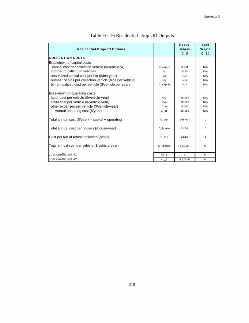
Appendix D
210
Table D - 16 Residential Drop Off Outputs
Recyc- Yard
Residential Drop-off Options labels Waste
C_8 C_10
COLLECTION COSTS
Breakdown of capital costs capital cost per collection vehicle ($/vehicle-yr) C_cap_v 9,641 N/A
number of collection vehicles Nt 9.15 N/A
annualized capital cost per bin ($/bin-year) Cb N/A N/A
number of bins per collection vehicle (bins per vehicle) Nb N/A N/A
bin annualized cost per vehicle ($/vehicle per year) C_cap_b N/A N/A
Breakdown of operating costs labor cost per vehicle ($/vehicle-year) Cw 40,196 N/A
O&M cost per vehicle ($/vehicle-year) Cvo 30,822 N/A
other expenses per vehicle ($/vehicle-year) Coe 8,083 N/A
Annual operating cost ($/year) C_op 88,593 N/A
Total annual cost ($/year) -- capital + operating C_ann 908,077 0
Total annual cost per house ($/house-year) C_house 11.94 0
Cost per ton of refuse collected ($/ton) C_ton 72.16 0
Total annual cost per vehicle ($/vehicle-year) C_vehicle 99,198 0
cost coefficient #1 cc_1 0 0
cost coefficient #2 cc_2 9,122.91 0

Appendix D
211
Table D - 17 Residential Drop Off Outputs (Continued)
Recyc- Yard
Residential Drop-off Options labels Waste
C_8 C_10
Calculations for collection vehicle activitiesvolume of recyclables deposited at drop-off site per week (cy/week) vol_recyc 3817.90 N/A
collection vehicle trips per week (trips/week) Rt 207.49 N/A
travel time from drop-off site to facility (min/trip) Trf 20.00 N/A
travel time from garage to drop-off site (min/day-vehicle) Tgr 20.00 N/A
travel time from facility to garage (min/day-vehicle) Tfg 20.00 N/A
time per trip (m in/trip) -- load+travel+unload time Tc 75.00 N/A
trips per day per vehicle (trip/day-vehicle) RD 4.53 N/A
daily weight of refuse collected per vehicle (tons/day-vehicle) RefD 5.27 N/A
Collection vehicle activity times
travel time from garage to drop-off site in the morning(min/day-vehicle) Tgr 20.00 N/A
loading time at drop-off site (min/day-vehicle) LD 90.67 N/A
travel time between disposal facility and drop-off site (m in/day-vehicle) F_R 161.33 N/A
unloading time at disposal facility (m in/day-vehicle) UD 68.00 N/A
lunch time (min/day-vehicle) F1_ 30.00 N/A
break time (min/day-vehicle) F2_ 30.00 N/A
travel time from disposal facility to garage at end of day (min/day-vehicle) Tfg 20.00 N/A
actual working time (min/day-vehicle) 420.00 N/A
service hours per day (hours/day-vehicle) ShD 6.00 N/A
Daily m iles traveled per collection vehiclefrom garage to drop-off site in the morning (miles/day) Dgr 11.67 N/A
between drop-off site and disposal facility (m iles/day) DF_S 80.67 N/A
from disposal facility to garage at end of day (miles/day) Dfg 11.67 N/A
total (miles/day-vehicle) MiD 104.00 N/A
Daily fuel usage per collection vehicle
from garage to drop-off site in the morning (gallons/day) 2.33 N/A
loading at drop-off site (gallons/day) 1.51 N/A
between disposal facility and route (gallons/day-vehicle) 16.13 N/A
unloading at disposal facility (gallons/day) 1.13 N/A
from disposal facility to garage at end of day (gallons/day) 2.33 N/A
total (gallons/day-vehicle) FuelD 23.44 N/A
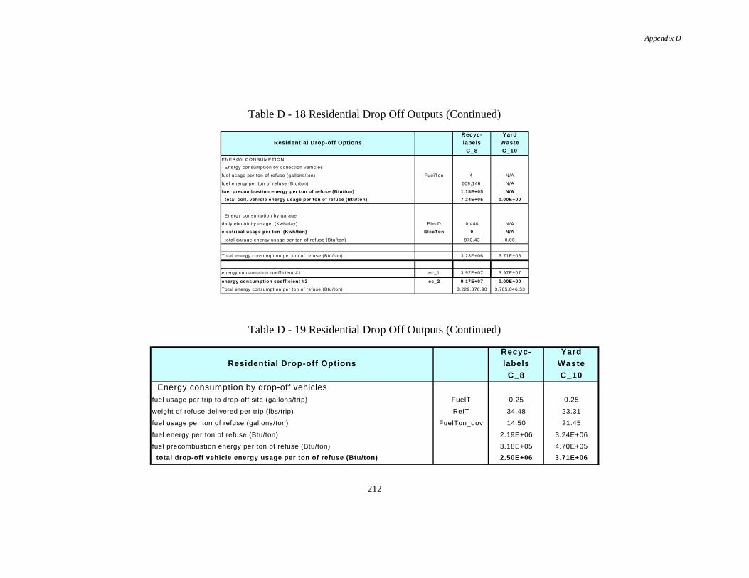
Appendix D
212
Table D - 18 Residential Drop Off Outputs (Continued)
Recyc- Yard
Residential Drop-off Options labels Waste
C_8 C_10
ENERGY CONSUMPTION
Energy consumption by collection vehicles
fuel usage per ton of refuse (gallons/ton) FuelTon 4 N/A
fuel energy per ton of refuse (Btu/ton) 609,146 N/A
fuel precombustion energy per ton of refuse (Btu/ton) 1.15E+05 N/A
total coll. vehicle energy usage per ton of refuse (Btu/ton) 7.24E+05 0.00E+00
Energy consumption by garage
daily electricity usage (Kwh/day) ElecD 0.440 N/A
electrical usage per ton (Kwh/ton) ElecTon 0 N/A
total garage energy usage per ton of refuse (Btu/ton) 870.43 0.00
Total energy consumption per ton of refuse (Btu/ton) 3.23E+06 3.71E+06
energy consumption coefficient #1 ec_1 3.97E+07 3.97E+07
energy consumption coefficient #2 ec_2 9.17E+07 0.00E+00
Total energy consumption per ton of refuse (Btu/ton) 3,229,870.90 3,705,046.53
Table D - 19 Residential Drop Off Outputs (Continued)
Recyc- Yard
Residential Drop-off Options labels Waste
C_8 C_10
Energy consumption by drop-off vehiclesfuel usage per trip to drop-off site (gallons/trip) FuelT 0.25 0.25
weight of refuse delivered per trip (lbs/trip) RefT 34.48 23.31
fuel usage per ton of refuse (gallons/ton) FuelTon_dov 14.50 21.45
fuel energy per ton of refuse (Btu/ton) 2.19E+06 3.24E+06
fuel precombustion energy per ton of refuse (Btu/ton) 3.18E+05 4.70E+05
total drop-off vehicle energy usage per ton of refuse (Btu/ton) 2.50E+06 3.71E+06

Appendix D
213
Table D - 20 Residential Drop Off Air Release Outputs
Recyc- YardResidential Drop-off Options labels Waste
C_8 C_10
AIRBORNE RELEASES
Carbon Monoxide
CO emissions from collection vehicles (lb/ton) 0.219 N/A
CO precombustion emissions from fuel production (lb/ton) 0.022 N/A
CO emissions from garage electricity generation (lb/ton) 1.78E-04 N/A
CO emissions from drop-off vehicles (lb/ton) 2.17460 3.21676
CO precombustion emissions from drop-off vehicles (lb/ton) 6.09E-02 9.01E-02
total CO releases per ton of refuse (lb/ton) 2.477 3.307
CO emission coefficient #1 CO_1 3.5473E+01 3.5473E+01
CO emission coefficient #2 CO_2 3.05E+01 0.00E+00
total CO releases per ton of refuse (lb/ton) 2.477 3.307
Nitrogen Oxides
NOx emissions from collection vehicles (lb/ton) 1.480 N/A
NOx precombustion emissions from fuel production (lb/ton) 0.032 N/A
NOx emissions from garage electricity generation (lb/ton) 5.39E-04 N/A
NOx emissions from drop-off vehicles (lb/ton) 0.63959 0.94611
NOx precombustion emissions from drop-off vehicles (lb/ton) 8.79E-02 1.30E-01
total NOx releases per ton of refuse (lb/ton) 2.240 1.076
NOx emission coefficient #1 NO_1 1.15E+01 1.15E+01
NOx emission coefficient #2 NO_2 1.91E+02 0.00E+00
total NOx releases per ton of refuse (lb/ton) 2.240 1.076
Particulate Matter
PM emissions from collection vehicles (lb/ton) 0.011 N/A
PM precombustion emissions from fuel production (lb/ton) 0.008 N/A
PM emissions from garage electricity generation (lb/ton) 2.17E-04 N/A
PM emissions from drop-off vehicles (lb/ton) 0.00 0.00
PM precombustion emissions from drop-off vehicles (lb/ton) 0.02 0.03
total PM releases per ton of refuse (lb/ton) 0.042 0.033
PM emission coefficient #1 PM_1 3.54E-01 3.54E-01
PM emission coefficient #2 PM_2 2.43E+00 0.00E+00
Table D - 21 Residential Drop Off Air Release Outputs (Continued)
Recyc- Yard
Residential Drop-off Options labels WasteC_8 C_10
PM10
PM10 emissions from collection vehicles (lb/ton) 0.000 N/A
PM10 precombustion emissions from fuel production (lb/ton) 0.000 N/A
PM10 emissions from garage electricity generation (lb/ton) 0.00E+00 N/A
PM10 emissions from drop-off vehicles (lb/ton) 0.12792 0.18922
PM10 precombustion emissions from drop-off vehicles (lb/ton) 0.00E+00 0.00E+00
total PM10 releases per ton of refuse (lb/ton) 0.128 0.189
PM10 emission coefficient #1 PM10_1 2.03E+00 2.03E+00
PM10 emission coefficient #2 PM10_2 0.00E+00 0.00E+00
total PM10 releases per ton of refuse (lb/ton) 0.128 0.189
Fossil CO2
CO2-fossil emissions from collection vehicles (lb/ton) 0.000 N/A
CO2-fossil precombustion emissions from fuel production (lb/ton) 15.980 N/A
CO2-fossil emissions from garage electricity generation (lb/ton) 1.24E-01 N/A
CO2-fossil emissions from drop-off vehicles (lb/ton) 0.00000 0.00000
CO2-fosssil precombustion emissions from drop-off vehicles (lb/ton) 4.40E+01 6.51E+01
total CO2-fossil releases per ton of refuse (lb/ton) 60.107 65.090
CO2-fossil emission coefficient #1 CO2f_1 6.98E+02 6.98E+02
CO2-fossil emission coefficient #2 CO2f_2 2.04E+03 0.00E+00
total CO2-fossil releases per ton of refuse (lb/ton) 60.107 65.090
Biomass CO2
CO2-biomass emissions from collection vehicles (lb/ton) 0.000 N/A
CO2-biomass precombustion emissions from fuel production (lb/ton) 0.000 N/A
CO2-biomass emissions from garage electricity generation (lb/ton) 0.00E+00 N/A
CO2-biomass emissions from drop-off vehicles (lb/ton) 0.00000 0.00000
CO2-biomass precombustion emissions from drop-off vehicles (lb/ton) 0.00E+00 0.00E+00
total CO2-biomass releases per ton of refuse (lb/ton) 0.00E+00 0.00E+00
CO2-biomass emission coefficient #1 CO2bm_1 0.00E+00 0.00E+00
CO2-biomass emission coefficient #2 CO2bm_2 0.00E+00 0.00E+00
total CO2-biomass releases per ton of refuse (lb/ton) 0.00E+00 0.00E+00

Appendix D
214
Table D - 22 Residential Drop Off Air Release Outputs (Continued)
Recyc- Yard
Residential Drop-off Options labels Waste
C_8 C_10
Sulfur Oxides
SOx emissions from collection vehicles (lb/ton) 0.000 N/A
SOx precombustion emissions from fuel production (lb/ton) 0.039 N/A
SOx emissions from garage electricity generation (lb/ton) 1.14E-03 N/A
SOx emissions from drop-off vehicles (lb/ton) 0.00000 0.00000
SOx precombustion emissions from drop-off vehicle fuel production (lb/ton) 1.08E-01 1.60E-01
total SOx releases per ton refuse (lb/ton) 0.148 0.160
SOx emission coefficient #1 SOx_1 1.71E+00 1.71E+00
SOx emission coefficient #2 SOx_2 5.09E+00 0.00E+00
total SOx releases per ton refuse (lb/ton) 0.148 0.160
Hydrocarbons (less methane)
HC emissions from collection vehicles (lb/ton) 0.027 N/A
HC precombustion emissions from collection vehicles (lb/ton) 0.300 N/A
HC emissions from garage electricity generation (lb/ton) 8.53E-05 N/A
HC emissions from drop-off vehicles (lb/ton) 2.62E-01 3.88E-01
HC precombustion emissions from drop-off vehicles (lb/ton) 8.31E-01 1.23E+00
total HC releases per ton of refuse (lb/ton) 1.420 1.617
HC emission coefficient #1 HC_1 1.73E+01 1.73E+01
HC emission coefficient #2 HC_2 4.13E+01 0.00E+00
Methane
CH4 emissions from collection vehicles (lb/ton) 0.000 N/A
CH4 precombustion emissions from fuel production (lb/ton) 2.22E-04 N/A
CH4 emissions from garage electricity generation (lb/ton) 8.22E-07 N/A
CH4 emissions from drop-off vehicles (lb/ton) 0.00E+00 0.00E+00
CH4 precombustion emissions from drop-off vehicle fuel production (lb/ton) 6.24E-04 9.23E-04
total CH4 releases per ton of refuse (lb/ton) 0.001 0.001
CH4 emission coefficient #1 CH4_1 9.90E-03 9.90E-03
CH4 emission coefficient #2 CH4_2 2.82E-02 0.00E+00
Table D - 23 Residential Drop Off Air Release Outputs (Continued)
Recyc- Yard
Residential Drop-off Options labels Waste
C_8 C_10
Lead
Lead emissions from collection vehicles (lb/ton) 0.000 N/A
Lead precombustion emissions from fuel production (lb/ton) 4.89E-08 N/A
Lead emissions from garage electricity generation (lb/ton) 4.09E-12 N/A
Lead emissions from drop-off vehicles (lb/ton) 0.00E+00 0.00E+00
Lead precombustion emissions from drop-off vehicle fuel production (lb/ton) 1.32E-07 1.95E-07
total Lead releases per ton of refuse ( lb/ton) 1.81E-07 1.95E-07
Pb emission coefficient #1 Pb_a_1 2.09E-06 2.09E-06
PB emission coefficient #2 Pb_a_2 1.10E-04 0.00E+00
Ammonia
Ammonia emissions from collection vehicles (lb/ton) 0.000 N/A
Ammonia precombustion emissions from fuel production (lb/ton) 1.73E-04 N/A
Ammonia emissions from garage electricity generation (lb/ton) 1.47E-08 N/A
Ammonia emissions from drop-off vehicles (lb/ton) 0.00E+00 0.00E+00
Ammonia precombustion emissions from drop-off vehicle fuel production (lb/ton) 4.79E-04 7.08E-04
total ammonia releases from refuse ( lb/ton) 6.52E-04 7.08E-04
NH3 emission coefficient #1 NH3_1 2.09E-06 2.09E-06
NH3 emission coefficient #2 NH3_2 1.10E-04 0.00E+00
Hydrochloric Acid
HCl emissions from collection vehicles (lb/ton) 0.000 N/A
HCl precombustion emissions from fuel production (lb/ton) 5.34E-06 N/A
HCl emissions from garage electricity generation (lb/ton) 4.43E-10 N/A
HCl emissions from drop-off vehicles (lb/ton) 0.00E+00 0.00E+00
total HCl releases from refuse ( lb/ton) 5.34E-06 0.00E+00
HCl emission coefficient #1 HCl_1 2.26E-04 2.26E-04
HCl emission coefficient #2 HCl_2 6.75E-04 0.00E+00

Appendix D
215
Table D - 24 Residential Drop Off Air Release Outputs (Continued)
Recyc- Yard
Residential Drop-off Options labels Waste
C_8 C_10
Greenhouse Gas Equivalence
Carbon dioxide (fossil fuel) 60.11 65.09
Carbon dioxide (biomass) 0.00 0.00
Methane 0.05 0.06
Nitrous oxide 604.68 290.55
Other hydrocarbons 0.00 0.00
total greenhouse gas equivalence per ton of refuse 664.84 355.70
GHE emission coefficient #1 GHE_1 3.82E+03 3.82E+03
GHE emission coefficient #2 GHE_2 5.37E+04 0.00E+00
Table D - 25 Residential Drop Off Water Release Outputs (Continued)
Recyc- Yard
Residential Drop-off Options labels Waste
C_8 C_10
WATERBORNE RELEASES
Dissolved Solids
Dissolved solids emissions from washdown water (lb/ton) 0.00E+00 N/A
DS precombustion emissions from fuel production (lb/ton) 4.54E-01 N/A
DS emissions from garage electricity generation (lb/ton) 3.81E-05 N/A
DS precombustion emissions from drop-off vehicle fuel (lb/ton) 1.26E+00 1.86E+00
total dissolved solids releases per ton of refuse (lb/ton) 1.71E+00 1.86E+00
DS emission coefficient #1 DS_1 19.99890411 19.99890411
DS emission coefficient #2 DS_2 57.34177796 0
DS emission coefficient #3 DS_3 0.00E+00 0.00E+00
Suspended Solids
Suspended solids emissions from washdown water (lb/ton) 0.00E+00 N/A
SS precombustion emissions from fuel production (lb/ton) 4.22E-04 N/A
SS emissions from garage electricity generation (lb/ton) 3.43E-08 N/A
SS precombustion emissions from drop-off vehicle fuel (lb/ton) 1.17E-03 1.74E-03
total suspended solids releases per ton of refuse (lb/ton) 1.60E-03 1.74E-03
SS emission coefficient #1 SS_1 0.018641096 0.018641096
SS emission coefficient #2 SS_2 0.053406409 0
SS emission coefficient #3 SS_3 0.00E+00 0.00E+00
Biochemical Oxygen Demand
BOD emissions from washdown water (lb/ton) 0.00E+00 N/A
BOD precombustion emissions from fuel production (lb/ton) 4.45E-04 N/A
BOD emissions from garage electricity generation (lb/ton) 3.76E-08 N/A
BOD precombustion emissions from drop-off vehicle fuel (lb/ton) 1.29E-03 1.91E-03
total BOD releases per ton of refuse (lb/ton) 1.74E-03 1.91E-03
BOD emission coefficient #1 BOD_1 0.020482192 0.020482192
BOD emission coefficient #2 BOD_2 0.05621746 0
BOD emission coefficient #3 BOD_3 0.00E+00 0.00E+00

Appendix D
216
Table D - 26 Residential Drop Off Water Release Outputs (Continued)
Recyc- Yard
Residential Drop-off Options labels Waste
C_8 C_10
Chemical Oxygen Demand
COD emissions from washdown water (lb/ton) 0.00E+00 N/A
COD precombustion emissions from fuel production (lb/ton) 2.18E-03 N/A
COD emissions from garage electricity generation (lb/ton) 1.86E-07 N/A
COD precombustion emissions from drop-off vehicle fuel (lb/ton) 6.10E-03 9.02E-03
total COD releases per ton of refuse (lb/ton) 8.28E-03 9.02E-03
COD emission coefficient #1 COD_1 0.096772603 0.096772603
COD emission coefficient #2 COD_2 0.275791824 0
COD emission coefficient #3 COD_3 0.00E+00 0.00E+00
Oil
Oil emissions from washdown water (lb/ton) 0.00E+00 N/A
Oil precombustion emissions from fuel production (lb/ton) 5.47E-03 N/A
Oil emissions from garage electricity generation (lb/ton) 5.10E-07 N/A
Oil precombustion emissions from drop-off vehicle fuel (lb/ton) 1.52E-02 2.25E-02
total oil releases per ton of refuse (lb/ton) 2.07E-02 2.25E-02
oil emission coefficient #1 oil_1 0.241643836 0.241643836
oil emission coefficient #2 oil_2 0.69148071 0
oil emission coefficient #3 oil_3 0.00E+00 0.00E+00
Sulfuric Acid
Sulfuric acid emissions from washdown water (lb/ton) 0.00E+00 N/A
Sulfuric acid precombustion emissions from fuel production (lb/ton) 1.38E-03 N/A
Sulfuric acid emissions from garage electricity generation (lb/ton) 9.37E-05 N/A
Sulfuric acid precombustion emissions from drop-off vehicle fuel (lb/ton) 3.77E-03 5.58E-03
total sulfuric acid releases per ton of refuse (lb/ton) 5.24E-03 5.58E-03
H2SO4 emission coefficient #1 H2SO4_1 0.059835616 0.059835616
H2SO4 emission coefficient #2 H2SO4_2 0.186107528 0
H2SO4 emission coefficient #3 H2SO4_3 0.00E+00 0.00E+00
Table D - 27 Residential Drop Off Water Release Outputs (Continued)
Recyc- Yard
Residential Drop-off Options labels Waste
C_8 C_10
Iron
Iron emissions from washdown water (lb/ton) 0.00E+00 N/A
Iron precombustion emissions from fuel production (lb/ton) 3.60E-04 N/A
Iron emissions from garage electricity generation (lb/ton) 2.33E-05 N/A
Iron precombustion emissions from drop-off vehicle fuel (lb/ton) 9.86E-04 1.46E-03
total iron releases per ton of refuse (lb/ton) 1.37E-03 1.46E-03
fe emission coefficient #1 fe_1 0.015649315 0.015649315
fe emission coefficient #2 fe_2 0.048479732 0
fe emission coefficient #3 fe_3 0.00E+00 0.00E+00
Ammonia
Ammonia emissions from washdown water (lb/ton) 0.00E+00 N/A
Ammonia precombustion emissions from fuel production (lb/ton) 6.22E-05 N/A
Ammonia emissions from garage electricity generation (lb/ton) 5.13E-09 N/A
Ammonia precombustion emissions from drop-off vehicle fuel (lb/ton) 1.74E-04 2.57E-04
total ammonia releases per ton of refuse (lb/ton) 2.36E-04 2.57E-04
NH4 emission coefficient #1 NH4_1 0.002761644 0.002761644
NH4 emission coefficient #2 NH4_2 0.007870427 0
NH4 emission coefficient #3 NH4_3 0.00E+00 0.00E+00
Copper
Copper emissions from washdown water (lb/ton) 0.00E+00 N/A
Copper precombustion emissions from fuel production (lb/ton) 0.00E+00 N/A
Copper emissions from garage electricity generation (lb/ton) 0.00E+00 N/A
Copper precombustion emissions from drop-off vehicle fuel (lb/ton) 0.00E+00 0.00E+00
total copper releases per ton of refuse (lb/ton) 0.00E+00 0.00E+00
cu emission coefficient #1 cu_1 0 0
cu emission coefficient #2 cu_2 0 0
cu emission coefficient #3 cu_3 0.00E+00 0.00E+00

Appendix D
217
Table D - 28 Residential Drop Off Water Release Outputs (Continued)
Recyc- Yard
Residential Drop-off Options labels Waste
C_8 C_10
Cadmium
Cadmium emissions from washdown water (lb/ton) 0.00E+00 N/A
Cadmium precombustion emissions from fuel production (lb/ton) 0.00E+00 N/A
Cadmium emissions from garage electricity generation (lb/ton) 0.00E+00 N/A
Cadmium precombustion emissions from drop-off vehicle fuel (lb/ton) 0.00E+00 0.00E+00
total cadmium releases per ton of refuse (lb/ton) 0.00E+00 0.00E+00
cd emission coefficient #1 cd_1 0 0
cd emission coefficient #2 cd_2 0 0
cd emission coefficient #3 cd_3 0.00E+00 0.00E+00
Arsenic
Arsenic emissions from washdown water (lb/ton) 0.00E+00 N/A
Arsenic precombustion emissions from fuel production (lb/ton) 0.00E+00 N/A
Arsenic emissions from garage electricity generation (lb/ton) 0.00E+00 N/A
Arsenic precombustion emissions from drop-off vehicle fuel (lb/ton) 0.00E+00 0.00E+00
total arsenic releases per ton of refuse (lb/ton) 0.00E+00 0.00E+00
as emission coefficient #1 as_1 0 0
as emission coefficient #2 as_2 0 0
as emission coefficient #3 as_3 0.00E+00 0.00E+00
Mercury
Mercury emissions from washdown water (lb/ton) 0.00E+00 N/A
Mercury precombustion emissions from fuel production (lb/ton) 0.00E+00 N/A
Mercury emissions from garage electricity generation (lb/ton) 0.00E+00 N/A
Mercury precombustion emissions from drop-off vehicle fuel (lb/ton) 0.00E+00 0.00E+00
total mercury releases per ton of refuse (lb/ton) 0.00E+00 0.00E+00
hg emission coefficient #1 hg_1 0 0
hg emission coefficient #2 hg_2 0 0
hg emission coefficient #3 hg_3 0.00E+00 0.00E+00
Table D - 29 Residential Drop Off Water Release Outputs (Continued)
Recyc- Yard
Residential Drop-off Options labels Waste
C_8 C_10
Phosphate
Phosphate emissions from washdown water (lb/ton) 0.00E+00 N/A
Phosphate precombustion emissions from fuel production (lb/ton) 0.00E+00 N/A
Phosphate emissions from garage electricity generation (lb/ton) 0.00E+00 N/A
Phosphate precombustion emissions from drop-off vehicle fuel (lb/ton) 0.00E+00 0.00E+00
total phosphate releases per ton of refuse (lb/ton) 0.00E+00 0.00E+00
po4 emission coefficient #1 po4_1 0 0
po4 emission coefficient #2 po4_2 0 0
po4 emission coefficient #3 po4_3 0.00E+00 0.00E+00
Selenium
Selenium emissions from washdown water (lb/ton) 0.00E+00 N/A
Selenium precombustion emissions from fuel production (lb/ton) 0.00E+00 N/A
Selenium emissions from garage electricity generation (lb/ton) 0.00E+00 N/A
Selenium precombustion emissions from drop-off vehicle fuel (lb/ton) 0.00E+00 0.00E+00
total selenium releases per ton of refuse (lb/ton) 0.00E+00 0.00E+00
se emission coefficient #1 se_1 0 0
se emission coefficient #2 se_2 0 0
se emission coefficient #3 se_3 0.00E+00 0.00E+00
Chromium
Chromium emissions from washdown water (lb/ton) 0.00E+00 N/A
Chromium precombustion emissions from fuel production (lb/ton) 1.51E-07 N/A
Chromium emissions from garage electricity generation (lb/ton) 5.92E-12 N/A
Chromium precombustion emissions from drop-off vehicle fuel (lb/ton) 0.00E+00 0.00E+00
total chromium releases per ton of refuse (lb/ton) 1.51E-07 0.00E+00
cr emission coefficient #1 cr_1 0 0
cr emission coefficient #2 cr_2 1.91131E-05 0
cr emission coefficient #3 cr_3 0.00E+00 0.00E+00

Appendix D
218
Table D - 30 Residential Drop Off Water Release Outputs (Continued)
Recyc- Yard
Residential Drop-off Options labels Waste
C_8 C_10
Lead
Lead emissions from washdown water (lb/ton) 0.00E+00 N/A
Lead precombustion emissions from fuel production (lb/ton) 6.67E-08 N/A
Lead emissions from garage electricity generation (lb/ton) 5.49E-12 N/A
Lead precombustion emissions from drop-off vehicle fuel (lb/ton) 1.89E-07 2.79E-07
total lead releases per ton of refuse (lb/ton) 2.55E-07 2.79E-07
pb emission coefficient #1 pb_1 2.99178E-06 2.99178E-06
pb emission coefficient #2 pb_2 8.4326E-06 0
pb emission coefficient #3 pb_3 0.00E+00 0.00E+00
Zinc
Zinc emissions from washdown water (lb/ton) 0.00E+00 N/A
Zinc precombustion emissions from fuel production (lb/ton) 9.78E-07 N/A
Zinc emissions from garage electricity generation (lb/ton) 8.20E-11 N/A
Zinc precombustion emissions from drop-off vehicle fuel (lb/ton) 2.76E-06 4.08E-06
Total zinc releases per ton of refuse (lb/ton) 3.73E-06 4.08E-06
zn emission coefficient #1 zn_1 4.3726E-05 4.3726E-05
zn emission coefficient #2 zn_2 0.000123678 0
zn emission coefficient #3 zn_3 0.00E+00 0.00E+00
Table D - 31 Residential Drop Off Solid Waste Outputs (Continued)
Recyc- Yard
Residential Drop-off Options labels Waste
C_8 C_10
SOLID WASTE
Solid Waste #1
SW#1 precombustion emissions from fuel production (lb/ton) 3.66E-01 N/A
SW#1 emissions from garage electricity generation (lb/ton) 1.59E-02 N/A
SW#1 precombustion emissions from drop-off vehicle fuel production (lb/ton) 1.01E+00 1.50E+00
total SW#1 generation per ton of refuse (lb/ton) 1.39E+00 1.50E+00
SW1 emission coefficient #1 SW1_1 1.60E+01 1.60E+01
SW1 emission coefficient #2 SW1_2 4.83E+01 0.00E+00
Solid Waste #2
SW #2 precombustion emissions from fuel production (lb/ton) 0.00E+00 N/A
SW #2 emissions from garage electricity generation (lb/ton) 0.00E+00 N/A
SW #2 precombustion emissions from drop-off vehicle fuel production (lb/ton) 0.00E+00 0.00E+00
total SW #2 generation per ton of refuse (lb/ton) 0.00E+00 0.00E+00
SW2 emission coefficient #2 SW2_2 0.00E+00 0.00E+00
Solid Waste #3
SW #3 precombustion emissions from fuel production (lb/ton) 0.00E+00 N/A
SW #3 emissions from garage electricity generation (lb/ton) 0.00E+00 N/A
SW #3 precombustion emissions from drop-off vehicle fuel production (lb/ton) 0.00E+00 0.00E+00
total SW #3 generation per ton of refuse (lb/ton) 0.00E+00 0.00E+00
SW3 emission coefficient #1 SW3_1 0.00E+00 0.00E+00
SW3 emission coefficient #2 SW3_2 0.00E+00 0.00E+00
Solid Waste #4
SW #4 precombustion emissions from fuel production (lb/ton) 0.00E+00 N/A
SW #4 emissions from garage electricity generation (lb/ton) 0.00E+00 N/A
SW #4 precombustion emissions from drop-off vehicle fuel production (lb/ton) 0.00E+00 0.00E+00
total SW #4 generation per ton of refuse (lb/ton) 0.00E+00 0.00E+00
SW4 emission coefficient #1 SW4_1 0.00E+00 0.00E+00
SW4 emission coefficient #2 SW4_2 0.00E+00 0.00E+00
Solid Waste #5
SW #5 precombustion emissions from fuel production (lb/ton) 0.00E+00 N/A
SW #5 emissions from garage electricity generation (lb/ton) 0.00E+00 N/A
SW #5 precombustion emissions from drop-off vehicle fuel production (lb/ton) 0.00E+00 0.00E+00
total SW #5 generation per ton of refuse (lb/ton) 0.00E+00 0.00E+00
SW5 emission coefficient #1 SW5_1 0.00E+00 0.00E+00
SW5 emission coefficient #2 SW5_2 0.00E+00 0.00E+00

Appendix D
219
Table D - 32 Multi-Family Collection Outputs
M ixed Resi- Recyclables
Multi-Fam ily Collection Options Waste duals Wet/Dry
C_13 C_16 C_17 C_18 C_14 C_15
COLLECTION COSTS
Breakdown of capital costs annualized capital cost per vehicle ($/vehicle-year) C_cap_v 25,845 25,845 27,999 25,845 9,641 23,138
number of collection vehicles (vehicles) Nt 2.05 1.67 4.44 1.67 2.07 2.01
annualized capital cost per bin ($/bin-year) Cb 17.33 17.33 17.33 17.33
number of bins per collection vehicle (bins per vehicle) Nb 68 119 193 40
bin annualized cost per vehicle ($/vehicle per year) C_cap_b 1,171 2,070 3,347 689
Breakdown of operating costs labor cost per vehicle ($/vehicle-year) Cw 69,170 69,170 69,170 69,170 40,196 69,170
O&M cost per vehicle ($/vehicle-year) Cvo 29,376 29,376 33,381 29,376 30,822 29,376
other expenses per vehicle ($/vehicle-year) Coe 16,166 16,166 16,166 16,166 8,083 16,166
Annual operating cost ($/year) C_op 128,477 128,477 132,964 128,477 88,593 128,477
Total annual cost ($/year) -- capital + operating C_ann 321,726 262,738 731,998 266,204 212,370 310,971
Total annual cost per collection location ($/location-year) C_location 3,217.26 2,627.38 7,319.98 2,662.04 2,123.70 3,109.71
Cost per ton of refuse collected ($/ton) C_ton 30.61 32.54 69.63 16.49 90.21 123.28
Total annual cost per vehicle ($/vehicle-year) C_vehicle 156,907 156,907 164,934 158,976 102,545 154,619
cost coefficient #1 cc_1 25,863.94 25,863.94 29,212.94 27,193.28 32,493.93 45,555.71
cost coefficient #2 cc_2 13,305.01 13,305.01 15,310.65 13,305.01 8,064.65 11,350.05

Appendix D
220
Table D - 33 Multi-Family Collection Outputs (Continued)
M ixed Resi- Recyclables
Multi-Fam ily Collection Options Waste duals W e t/Dry
C_13 C_16 C_17 C_18 C_14 C_15
Calculations for collection vehicle activities
locations per trip Ht 2.18 2.84 0.97 2.84 2.14 2.02
travel time between collection locations (min/stop) Tbet 1.50 1.50 1.50 1.50 1.50 1.50
travel time from collection route to disposal facility (min/trip) Trf 20.00 20.00 20.00 20.00 20.00 20.00
travel time from garage to first collection route (min/day-vehicle) Tgr 20.00 20.00 20.00 20.00 20.00 20.00
travel time from disposal facility to garage (m in/day-vehicle) Tfg 20.00 20.00 20.00 20.00 20.00 20.00
time per trip (m in/trip) -- collection+travel+unload time Tc 67.69 71.97 64.83 71.97 83.11 76.70
trips per day per vehicle (trips/day-vehicle) RD 4.47 4.20 4.63 4.20 3.61 3.94
daily weight of refuse collected per vehicle (tons/day) RefD 19.66 18.49 9.08 36.99 4.36 4.81
number of collection stops per day (stops/vehicle-day) SD 9.75 11.94 4.51 11.94 7.73 7.96
Collection vehicle activity times
travel time from garage to first collection route (min/day-vehicle) Tgr 20.00 20.00 20.00 20.00 20.00 20.00
loading time at collection stops (min/day-vehicle) LD 48.77 59.72 22.53 59.72 77.26 79.55
travel time between collection stops (min/day-vehicle) Tb 7.93 11.61 -0.18 11.61 6.17 6.02
travel time between disposal facility and route (m in/day-vehicle) F_R 188.77 178.12 195.10 178.12 154.38 167.77
unloading time at disposal facility (m in/day-vehicle) UD 74.54 70.55 102.55 70.55 82.19 66.66
lunch time (min/day-vehicle) F1_ 30.00 30.00 30.00 30.00 30.00 30.00
break time (min/day-vehicle) F2_ 30.00 30.00 30.00 30.00 30.00 30.00
travel time from disposal facility to garage (m in/day-vehicle) Tfg 20.00 20.00 20.00 20.00 20.00 20.00
actual working time (min/day-vehicle) 420.00 420.00 420.00 420.00 420.00 420.00
service hours per day (hours/day-vehicle) ShD 6.00 6.00 6.00 6.00 6.00 6.00
Daily m iles traveled per collection vehiclefrom garage to first collection route (m iles/day) Dgr 11.67 11.67 11.67 11.67 11.67 11.67
between collection stops (miles/day) Db 1.32 1.94 -0.03 1.94 1.03 1.00
between disposal facility and route (m iles/day) DF_R 94.38 89.06 97.55 89.06 77.19 83.88
from disposal facility to garage (m iles/day) Dfg 11.67 11.67 11.67 11.67 11.67 11.67
total (miles/day) Mi 119.04 114.33 120.85 114.33 101.55 108.22
Daily fuel usage per collection vehicle
from garage to first collection route (gallons/day) 2.33 2.33 2.33 2.33 2.33 2.33
loading at collection stops (gallons/day) 0.81 1.00 0.38 1.00 1.29 1.33
between collection stops (gallons/day) 0.66 0.97 -0.02 0.97 0.51 0.50
between disposal facility and route (gallons/day) 18.88 17.81 19.51 17.81 15.44 16.78
unloading at disposal facility (gallons/day) 1.24 1.18 1.71 1.18 1.37 1.11
from disposal facility to garage (gallons/day) 2.33 2.33 2.33 2.33 2.33 2.33
total (gallons/day) FuelD 26.26 25.62 26.25 25.62 23.28 24.38

Appendix D
221
Table D - 34 Multi-Family Collection Outputs (Continued)
M ixed Resi- Recyclables 0
M u lti-Fam ily Collection Options Waste duals W e t/Dry 0
C_13 C_16 C_17 C_18 C_14 C_15
ENERGY CONSUMPTION
Energy consumption by collection vehicles
fuel usage per ton of refuse (gallons/ton) FuelTon 1 1 3 1 5 5
fuel energy per ton of refuse (Btu/ton) 182,946 189,776 395,792 94,888 731,352 694,325
fuel precombustion energy per ton of refuse (Btu/ton) 3.46E+04 3.59E+04 7.48E+04 1.79E+04 1.38E+05 1.31E+05
total coll. vehicle energy usage per ton of refuse (Btu/ton) 2.18E+05 2.26E+05 4.71E+05 1.13E+05 8.70E+05 8.26E+05
Energy consumption by garage
daily electricity usage (kWh/day) ElecD 0.440 0.440 0.440 0.440 0.440 0.440
electricity usage per ton of refuse (kWh/ton) 0 0 0 0 0 0
total garage energy usage per ton of refuse (Btu/ton) 233.40 248.17 505.19 124.09 1,052.59 954.00
Total energy consumption per ton of refuse (Btu/ton) 2.18E+05 2.26E+05 4.71E+05 1.13E+05 8.71E+05 8.27E+05
energy consumption coefficient #1 ec_1 1.09E+08 1.09E+08 1.09E+08 1.09E+08 1.68E+08 1.67E+08
energy consumption coefficient #2 ec_2 1.05E+08 1.05E+08 1.09E+08 1.05E+08 9.48E+07 9.13E+07
Total energy consumption per ton of refuse (Btu/ton) 217,764.95 225,901.18 471,122.18 112,950.59 870,667.99 826,541.48

Appendix D
222
Table D - 35 Multi-Family Collection Air Release Outputs
M ixed Resi- Recyclables 0
M u lti-Fam ily Collection Options Waste duals W e t/Dry 0
C_13 C_16 C_17 C_18 C_14 C_15
AIRBORNE RELEASES
Carbon Monoxide
CO emissions from collection vehicles (lb/ton) 0.067 0.069 0.148 0.034 0.258 0.249
CO precombustion emissions from fuel production (lb/ton) 0.007 0.007 0.014 0.003 0.027 0.025
CO emissions from garage electricity generation (lb/ton) 4.78E-05 5.08E-05 1.03E-04 2.54E-05 2.15E-04 1.95E-04
total CO releases per ton of refuse (lb/ton) 0.074 0.076 0.162 0.038 0.285 0.275
CO emission coefficient #1 CO_1 2.2425E+01 2.2425E+01 2.2558E+01 2.2425E+01 3.4873E+01 3.4639E+01
CO emission coefficient #2 CO_2 3.76E+01 3.76E+01 3.84E+01 3.76E+01 3.34E+01 3.27E+01
total CO releases per ton of refuse (lb/ton) 0.074 0.076 0.162 0.038 0.285 0.275
Nitrogen Oxides
NOx emissions from collection vehicles (lb/ton) 0.454 0.464 0.998 0.232 1.747 1.687
NOx precombustion emissions from fuel production (lb/ton) 0.010 0.010 0.021 0.005 0.038 0.036
NOx emissions from garage electricity generation (lb/ton) 1.45E-04 1.54E-04 3.13E-04 7.68E-05 6.52E-04 5.91E-04
total NOx releases per ton of refuse (lb/ton) 0.464 0.474 1.019 0.237 1.786 1.724
NOx emission coefficient #1 NO_1 1.34E+02 1.34E+02 1.35E+02 1.34E+02 2.08E+02 2.07E+02
NOx emission coefficient #2 NO_2 2.37E+02 2.37E+02 2.42E+02 2.37E+02 2.10E+02 2.06E+02
total NOx releases per ton of refuse (lb/ton) 0.464 0.474 1.019 0.237 1.786 1.724
Particulate Matter
PM emissions from collection vehicles (lb/ton) 0.003 0.003 0.007 0.002 0.013 0.012
PM precombustion emissions from fuel production (lb/ton) 0.002 0.003 0.005 0.001 0.010 0.009
PM emissions from garage electricity generation (lb/ton) 5.81E-05 6.18E-05 1.26E-04 3.09E-05 2.62E-04 2.38E-04
total PM releases per ton of refuse (lb/ton) 0.006 0.006 0.013 0.003 0.023 0.022
PM emission coefficient #1 PM_1 2.21E+00 2.21E+00 2.22E+00 2.21E+00 3.44E+00 3.41E+00
PM emission coefficient #2 PM_2 2.90E+00 2.90E+00 2.99E+00 2.90E+00 2.60E+00 2.52E+00

Appendix D
223
Table D - 36 Multi-Family Collection Air Release Outputs (Continued)
M ixed Resi- Recyclables 0
M u lti-Fam ily Collection Options Waste duals W e t/Dry 0
C_13 C_16 C_17 C_18 C_14 C_15
PM10
PM10 emissions from collection vehicles (lb/ton) 0.000 0.000 0.000 0.000 0.000 0.000
PM10 precombustion emissions from fuel production (lb/ton) 0.000 0.000 0.000 0.000 0.000 0.000
PM10 emissions from garage electricity generation (lb/ton) 0.00E+00 0.00E+00 0.00E+00 0.00E+00 0.00E+00 0.00E+00
total PM10 releases per ton of refuse (lb/ton) 0.000 0.000 0.000 0.000 0.000 0.000
PM10 emission coefficient #1 PM10_1 0.00E+00 0.00E+00 0.00E+00 0.00E+00 0.00E+00 0.00E+00
PM10 emission coefficient #2 PM10_2 0.00E+00 0.00E+00 0.00E+00 0.00E+00 0.00E+00 0.00E+00
total PM10 releases per ton of refuse (lb/ton) 0.000 0.000 0.000 0.000 0.000 0.000
Fossil CO2
CO2-fossil emissions from collection vehicles (lb/ton) 0.000 0.000 0.000 0.000 0.000 0.000
CO2-fossil precombustion emissions from fuel production (lb/ton) 4.799 4.978 10.383 2.489 19.186 18.215
CO2-fossil emissions from garage electricity generation (lb/ton) 3.33E-02 3.54E-02 7.21E-02 1.77E-02 1.50E-01 1.36E-01
total CO2-fossil releases per ton of refuse (lb/ton) 4.833 5.014 10.455 2.507 19.336 18.351
CO2-fossil emission coefficient #1 CO2f_1 2.42E+03 2.42E+03 2.43E+03 2.42E+03 3.75E+03 3.73E+03
CO2-fossil emission coefficient #2 CO2f_2 2.33E+03 2.33E+03 2.42E+03 2.33E+03 2.10E+03 2.02E+03
total CO2-fossil releases per ton of refuse (lb/ton) 4.833 5.014 10.455 2.507 19.336 18.351
Biomass CO2
CO2-biomass emissions from collection vehicles (lb/ton) 0.000 0.000 0.000 0.000 0.000 0.000
CO2-biomass precombustion emissions from fuel production (lb/ton) 0.000 0.000 0.000 0.000 0.000 0.000
CO2-biomass emissions from garage electricity generation (lb/ton) 0.00E+00 0.00E+00 0.00E+00 0.00E+00 0.00E+00 0.00E+00
total CO2-biomass releases per ton of refuse (lb/ton) 0.00E+00 0.00E+00 0.00E+00 0.00E+00 0.00E+00 0.00E+00
CO2-biomass emission coefficient #1 CO2bm_1 0.00E+00 0.00E+00 0.00E+00 0.00E+00 0.00E+00 0.00E+00
CO2-biomass emission coefficient #2 CO2bm_2 0.00E+00 0.00E+00 0.00E+00 0.00E+00 0.00E+00 0.00E+00
total CO2-biomass releases per ton of refuse (lb/ton) 0.00E+00 0.00E+00 0.00E+00 0.00E+00 0.00E+00 0.00E+00

Appendix D
224
Table D - 37 Multi-Family Collection Air Release Outputs (Continued)
M ixed Resi- Recyclables 0
M u lti-Fam ily Collection Options Waste duals W e t/Dry 0
C_13 C_16 C_17 C_18 C_14 C_15
Sulfur Oxides
SOx emissions from collection vehicles (lb/ton) 0.000 0.000 0.000 0.000 0.000 0.000
SOx precombustion emissions from fuel production (lb/ton) 0.012 0.012 0.025 0.006 0.047 0.045
SOx emissions from garage electricity generation (lb/ton) 3.06E-04 3.25E-04 6.62E-04 1.63E-04 1.38E-03 1.25E-03
total SOx releases per ton refuse (lb/ton) 0.012 0.013 0.026 0.006 0.048 0.046
SOx emission coefficient #1 SOx_1 6.12E+00 6.12E+00 6.15E+00 6.12E+00 9.53E+00 9.47E+00
SOx emission coefficient #2 SOx_2 5.80E+00 5.80E+00 6.03E+00 5.80E+00 5.24E+00 5.04E+00
total SOx releases per ton refuse (lb/ton) 0.012 0.013 0.026 0.006 0.048 0.046
Hydrocarbons (less methane)
HC emissions from collection vehicles (lb/ton) 0.008 0.008 0.018 0.004 0.031 0.030
HC precombustion emissions from collection vehicles (lb/ton) 0.090 0.093 0.195 0.047 0.360 0.342
HC emissions from garage electricity generation (lb/ton) 2.29E-05 2.43E-05 4.95E-05 1.22E-05 1.03E-04 9.34E-05
total HC releases per ton of refuse (lb/ton) 0.098 0.102 0.213 0.051 0.392 0.372
HC emission coefficient #1 HC_1 4.72E+01 4.72E+01 4.75E+01 4.72E+01 7.32E+01 7.27E+01
HC emission coefficient #2 HC_2 4.76E+01 4.76E+01 4.94E+01 4.76E+01 4.29E+01 4.14E+01
Methane
CH4 emissions from collection vehicles (lb/ton) 0.000 0.000 0.000 0.000 0.000 0.000
CH4 precombustion emissions from fuel production (lb/ton) 6.68E-05 6.93E-05 1.44E-04 3.46E-05 2.67E-04 2.53E-04
CH4 emissions from garage electricity generation (lb/ton) 2.20E-07 2.34E-07 4.77E-07 1.17E-07 9.94E-07 9.01E-07
total CH4 releases per ton of refuse (lb/ton) 0.000 0.000 0.000 0.000 0.000 0.000
CH4 emission coefficient #1 CH4_1 3.35E-02 3.35E-02 3.37E-02 3.35E-02 5.19E-02 5.15E-02
CH4 emission coefficient #2 CH4_2 3.23E-02 3.23E-02 3.35E-02 3.23E-02 2.91E-02 2.81E-02

Appendix D
225
Table D - 38 Multi-Family Collection Air Release Outputs (Continued)
M ixed Resi- Recyclables 0
M u lti-Fam ily Collection Options Waste duals W e t/Dry 0
C_13 C_16 C_17 C_18 C_14 C_15
Lead
Lead emissions from collection vehicles (lb/ton) 0.000 0.000 0.000 0.000 0.000 0.000
Lead precombustion emissions from fuel production (lb/ton) 1.47E-08 1.52E-08 3.18E-08 7.62E-09 5.87E-08 5.57E-08
Lead emissions from garage electricity generation (lb/ton) 1.10E-12 1.17E-12 2.38E-12 5.84E-13 4.95E-12 4.49E-12
total lead releases per ton of refuse (lb/ton) 1.47E-08 1.52E-08 3.18E-08 7.62E-09 5.87E-08 5.58E-08
Pb emission coefficient #1 Pb_a_1 1.94E-04 1.94E-04 1.95E-04 1.94E-04 3.44E-04 3.41E-04
PB emission coefficient #2 Pb_a_2 1.03E-04 1.03E-04 1.13E-04 1.03E-04 9.82E-05 8.95E-05
Ammonia
Ammonia emissions from collection vehicles (lb/ton) 0.000 0.000 0.000 0.000 0.000 0.000
Ammonia precombustion emissions from fuel production (lb/ton) 5.21E-05 5.40E-05 1.13E-04 2.70E-05 2.08E-04 1.98E-04
Ammonia emissions from garage electricity generation (lb/ton) 3.94E-09 4.19E-09 8.53E-09 2.09E-09 1.78E-08 1.61E-08
total ammonia releases per ton of refuse (lb/ton) 5.21E-05 5.40E-05 1.13E-04 2.70E-05 2.08E-04 1.98E-04
NH3 emission coefficient #1 NH3_1 1.94E-04 1.94E-04 1.95E-04 1.94E-04 3.44E-04 3.41E-04
NH3 emission coefficient #2 NH3_2 1.03E-04 1.03E-04 1.13E-04 1.03E-04 9.82E-05 8.95E-05
Hydrochloric Acid
HCl emissions from collection vehicles (lb/ton) 0.000 0.000 0.000 0.000 0.000 0.000
HCl precombustion emissions from fuel production (lb/ton) 1.60E-06 1.66E-06 3.47E-06 8.31E-07 6.41E-06 6.08E-06
HCl emissions from garage electricity generation (lb/ton) 1.19E-10 1.26E-10 2.57E-10 6.32E-11 5.36E-10 4.86E-10
total HCl releases per ton of refuse (lb/ton) 1.60E-06 1.66E-06 3.47E-06 8.31E-07 6.41E-06 6.08E-06
HCl emission coefficient #1 HCl_1 7.99E-04 7.99E-04 8.03E-04 7.99E-04 1.24E-03 1.23E-03
HCl emission coefficient #2 HCl_2 7.72E-04 7.72E-04 8.02E-04 7.72E-04 6.97E-04 6.72E-04

Appendix D
226
Table D - 39 Multi-Family Collection Air Release Outputs (Continued)
M ixed Resi- Recyclables 0
M u lti-Fam ily Collection Options Waste duals W e t/Dry 0
C_13 C_16 C_17 C_18 C_14 C_15
Greenhouse Gas Equivalence
Carbon dioxide (fossil fuel) 4.83 5.01 10.46 2.51 19.34 18.35
Carbon dioxide (biomass) 0.00 0.00 0.00 0.00 0.00 0.00
Methane 0.00 0.00 0.01 0.00 0.02 0.02
Nitrous oxide 125.24 127.94 275.12 63.97 482.26 465.61
Other hydrocarbons 0.00 0.00 0.00 0.00 0.00 0.00
total greenhouse gas equivalence per ton of refuse 130.07 132.96 285.59 66.48 501.61 483.97
GHE emission coefficient #1 GHE_1 3.85E+04 3.85E+04 3.88E+04 3.85E+04 5.99E+04 5.95E+04
GHE emission coefficient #2 GHE_2 6.63E+04 6.63E+04 6.77E+04 6.63E+04 5.89E+04 5.76E+04
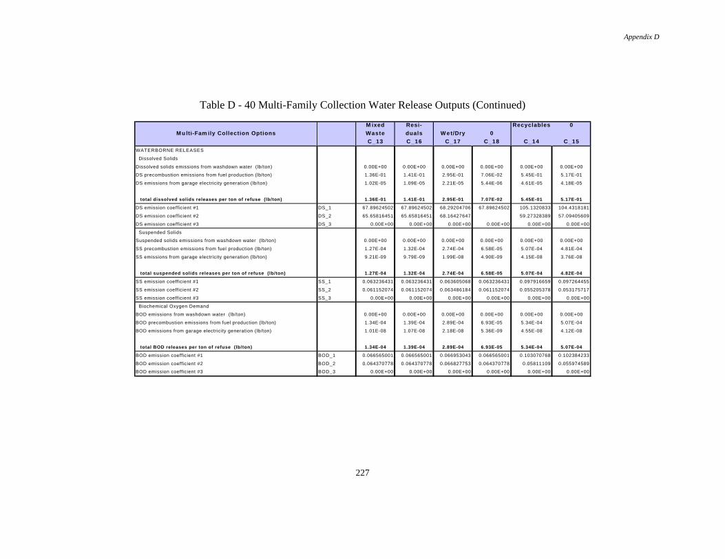
Appendix D
227
Table D - 40 Multi-Family Collection Water Release Outputs (Continued)
M ixed Resi- Recyclables 0
M u lti-Fam ily Collection Options Waste duals W e t/Dry 0
C_13 C_16 C_17 C_18 C_14 C_15
WATERBORNE RELEASES
Dissolved Solids
Dissolved solids emissions from washdown water (lb/ton) 0.00E+00 0.00E+00 0.00E+00 0.00E+00 0.00E+00 0.00E+00
DS precombustion emissions from fuel production (lb/ton) 1.36E-01 1.41E-01 2.95E-01 7.06E-02 5.45E-01 5.17E-01
DS emissions from garage electricity generation (lb/ton) 1.02E-05 1.09E-05 2.21E-05 5.44E-06 4.61E-05 4.18E-05
total dissolved solids releases per ton of refuse (lb/ton) 1.36E-01 1.41E-01 2.95E-01 7.07E-02 5.45E-01 5.17E-01
DS emission coefficient #1 DS_1 67.89624502 67.89624502 68.29204706 67.89624502 105.1320833 104.4318181
DS emission coefficient #2 DS_2 65.65816451 65.65816451 68.16427647 59.27328389 57.09405609
DS emission coefficient #3 DS_3 0.00E+00 0.00E+00 0.00E+00 0.00E+00 0.00E+00 0.00E+00
Suspended Solids
Suspended solids emissions from washdown water (lb/ton) 0.00E+00 0.00E+00 0.00E+00 0.00E+00 0.00E+00 0.00E+00
SS precombustion emissions from fuel production (lb/ton) 1.27E-04 1.32E-04 2.74E-04 6.58E-05 5.07E-04 4.81E-04
SS emissions from garage electricity generation (lb/ton) 9.21E-09 9.79E-09 1.99E-08 4.90E-09 4.15E-08 3.76E-08
total suspended solids releases per ton of refuse (lb/ton) 1.27E-04 1.32E-04 2.74E-04 6.58E-05 5.07E-04 4.82E-04
SS emission coefficient #1 SS_1 0.063236431 0.063236431 0.063605068 0.063236431 0.097916659 0.097264455
SS emission coefficient #2 SS_2 0.061152074 0.061152074 0.063486184 0.061152074 0.055205378 0.053175717
SS emission coefficient #3 SS_3 0.00E+00 0.00E+00 0.00E+00 0.00E+00 0.00E+00 0.00E+00
Biochemical Oxygen Demand
BOD emissions from washdown water (lb/ton) 0.00E+00 0.00E+00 0.00E+00 0.00E+00 0.00E+00 0.00E+00
BOD precombustion emissions from fuel production (lb/ton) 1.34E-04 1.39E-04 2.89E-04 6.93E-05 5.34E-04 5.07E-04
BOD emissions from garage electricity generation (lb/ton) 1.01E-08 1.07E-08 2.18E-08 5.36E-09 4.55E-08 4.12E-08
total BOD releases per ton of refuse (lb/ton) 1.34E-04 1.39E-04 2.89E-04 6.93E-05 5.34E-04 5.07E-04
BOD emission coefficient #1 BOD_1 0.066565001 0.066565001 0.066953043 0.066565001 0.103070768 0.102384233
BOD emission coefficient #2 BOD_2 0.064370778 0.064370778 0.066827753 0.064370778 0.05811109 0.055974589
BOD emission coefficient #3 BOD_3 0.00E+00 0.00E+00 0.00E+00 0.00E+00 0.00E+00 0.00E+00

Appendix D
228
Table D - 41 Multi-Family Collection Water Release Outputs (Continued)
M ixed Resi- Recyclables 0
M u lti-Fam ily Collection Options Waste duals W e t/Dry 0
C_13 C_16 C_17 C_18 C_14 C_15
Chemical Oxygen Demand
COD emissions from washdown water (lb/ton) 0.00E+00 0.00E+00 0.00E+00 0.00E+00 0.00E+00 0.00E+00
COD precombustion emissions from fuel production (lb/ton) 6.55E-04 6.80E-04 1.42E-03 3.40E-04 2.62E-03 2.49E-03
COD emissions from garage electricity generation (lb/ton) 4.99E-08 5.31E-08 1.08E-07 2.66E-08 2.25E-07 2.04E-07
total COD releases per ton of refuse (lb/ton) 6.55E-04 6.80E-04 1.42E-03 3.40E-04 2.62E-03 2.49E-03
COD emission coefficient #1 COD_1 0.326554955 0.326554955 0.328458613 0.326554955 0.505645239 0.502277229
COD emission coefficient #2 COD_2 0.315790354 0.315790354 0.327843803 0.315790354 0.285081568 0.274600308
COD emission coefficient #3 COD_3 0.00E+00 0.00E+00 0.00E+00 0.00E+00 0.00E+00 0.00E+00
Oil
Oil emissions from washdown water (lb/ton) 0.00E+00 0.00E+00 0.00E+00 0.00E+00 0.00E+00 0.00E+00
Oil precombustion emissions from fuel production (lb/ton) 1.64E-03 1.70E-03 3.55E-03 8.52E-04 6.57E-03 6.23E-03
Oil emissions from garage electricity generation (lb/ton) 1.37E-07 1.45E-07 2.96E-07 7.27E-08 6.17E-07 5.59E-07
total oil releases per ton of refuse (lb/ton) 1.64E-03 1.70E-03 3.55E-03 8.52E-04 6.57E-03 6.23E-03
oil emission coefficient #1 oil_1 0.81876018 0.81876018 0.823533182 0.81876018 1.267789476 1.259344935
oil emission coefficient #2 oil_2 0.791766054 0.791766054 0.821987415 0.791766054 0.714771665 0.688492221
oil emission coefficient #3 oil_3 0.00E+00 0.00E+00 0.00E+00 0.00E+00 0.00E+00 0.00E+00
Sulfuric Acid
Sulfuric acid emissions from washdown water (lb/ton) 0.00E+00 0.00E+00 0.00E+00 0.00E+00 0.00E+00 0.00E+00
Sulfuric acid precombustion emissions from fuel production (lb/ton) 4.14E-04 4.29E-04 8.96E-04 2.15E-04 1.65E-03 1.57E-03
Sulfuric acid emissions from garage electricity generation (lb/ton) 2.51E-05 2.67E-05 5.44E-05 1.34E-05 1.13E-04 1.03E-04
total sulfuric acid releases per ton of refuse (lb/ton) 4.39E-04 4.56E-04 9.50E-04 2.28E-04 1.77E-03 1.67E-03
H2SO4 emission coefficient #1 H2SO4_1 0.227561132 0.227561132 0.228940808 0.227561132 0.357356815 0.35491585
H2SO4 emission coefficient #2 H2SO4_2 0.210460134 0.210460134 0.219195871 0.210460134 0.190605106 0.183008812
H2SO4 emission coefficient #3 H2SO4_3 0.00E+00 0.00E+00 0.00E+00 0.00E+00 0.00E+00 0.00E+00

Appendix D
229
Table D - 42 Multi-Family Collection Water Release Outputs (Continued)
M ixed Resi- Recyclables 0
M u lti-Fam ily Collection Options Waste duals W e t/Dry 0
C_13 C_16 C_17 C_18 C_14 C_15
Iron
Iron emissions from washdown water (lb/ton) 0.00E+00 0.00E+00 0.00E+00 0.00E+00 0.00E+00 0.00E+00
Iron precombustion emissions from fuel production (lb/ton) 1.08E-04 1.12E-04 2.34E-04 5.61E-05 4.32E-04 4.11E-04
Iron emissions from garage electricity generation (lb/ton) 6.25E-06 6.65E-06 1.35E-05 3.32E-06 2.82E-05 2.56E-05
total iron releases per ton of refuse (lb/ton) 1.14E-04 1.19E-04 2.48E-04 5.94E-05 4.61E-04 4.36E-04
fe emission coefficient #1 fe_1 0.0591936 0.0591936 0.05955188 0.0591936 0.092899481 0.092265601
fe emission coefficient #2 fe_2 0.0548544 0.0548544 0.057122933 0.0548544 0.049672115 0.047699478
fe emission coefficient #3 fe_3 0.00E+00 0.00E+00 0.00E+00 0.00E+00 0.00E+00 0.00E+00
Ammonia
Ammonia emissions from washdown water (lb/ton) 0.00E+00 0.00E+00 0.00E+00 0.00E+00 0.00E+00 0.00E+00
Ammonia precombustion emissions from fuel production (lb/ton) 1.87E-05 1.94E-05 4.04E-05 9.70E-06 7.47E-05 7.10E-05
Ammonia emissions from garage electricity generation (lb/ton) 1.38E-09 1.46E-09 2.98E-09 7.31E-10 6.20E-09 5.62E-09
total ammonia releases per ton of refuse (lb/ton) 1.87E-05 1.94E-05 4.04E-05 9.70E-06 7.47E-05 7.10E-05
NH4 emission coefficient #1 NH4_1 0.009319069 0.009319069 0.009373394 0.009319069 0.014429852 0.014333737
NH4 emission coefficient #2 NH4_2 0.009011893 0.009011893 0.009355868 0.009011893 0.008135537 0.007836429
NH4 emission coefficient #3 NH4_3 0.00E+00 0.00E+00 0.00E+00 0.00E+00 0.00E+00 0.00E+00
Copper
Copper emissions from washdown water (lb/ton) 0.00E+00 0.00E+00 0.00E+00 0.00E+00 0.00E+00 0.00E+00
Copper precombustion emissions from fuel production (lb/ton) 0.00E+00 0.00E+00 0.00E+00 0.00E+00 0.00E+00 0.00E+00
Copper emissions from garage electricity generation (lb/ton) 0.00E+00 0.00E+00 0.00E+00 0.00E+00 0.00E+00 0.00E+00
total copper releases per ton of refuse (lb/ton) 0.00E+00 0.00E+00 0.00E+00 0.00E+00 0.00E+00 0.00E+00
cu emission coefficient #1 cu_1 0 0 0 0 0 0
cu emission coefficient #2 cu_2 0 0 0 0 0 0
cu emission coefficient #3 cu_3 0.00E+00 0.00E+00 0.00E+00 0.00E+00 0.00E+00 0.00E+00

Appendix D
230
Table D - 43 Multi-Family Collection Water Release Outputs (Continued)
M ixed Resi- Recyclables 0
M u lti-Fam ily Collection Options Waste duals W e t/Dry 0
C_13 C_16 C_17 C_18 C_14 C_15
Cadmium
Cadmium emissions from washdown water (lb/ton) 0.00E+00 0.00E+00 0.00E+00 0.00E+00 0.00E+00 0.00E+00
Cadmium precombustion emissions from fuel production (lb/ton) 0.00E+00 0.00E+00 0.00E+00 0.00E+00 0.00E+00 0.00E+00
Cadmium emissions from garage electricity generation (lb/ton) 0.00E+00 0.00E+00 0.00E+00 0.00E+00 0.00E+00 0.00E+00
total cadmium releases per ton of refuse (lb/ton) 0.00E+00 0.00E+00 0.00E+00 0.00E+00 0.00E+00 0.00E+00
cd emission coefficient #1 cd_1 0 0 0 0 0 0
cd emission coefficient #2 cd_2 0 0 0 0 0 0
cd emission coefficient #3 cd_3 0.00E+00 0.00E+00 0.00E+00 0.00E+00 0.00E+00 0.00E+00
Arsenic
Arsenic emissions from washdown water (lb/ton) 0.00E+00 0.00E+00 0.00E+00 0.00E+00 0.00E+00 0.00E+00
Arsenic precombustion emissions from fuel production (lb/ton) 0.00E+00 0.00E+00 0.00E+00 0.00E+00 0.00E+00 0.00E+00
Arsenic emissions from garage electricity generation (lb/ton) 0.00E+00 0.00E+00 0.00E+00 0.00E+00 0.00E+00 0.00E+00
total arsenic releases per ton of refuse (lb/ton) 0.00E+00 0.00E+00 0.00E+00 0.00E+00 0.00E+00 0.00E+00
as emission coefficient #1 as_1 0 0 0 0 0 0
as emission coefficient #2 as_2 0 0 0 0 0 0
as emission coefficient #3 as_3 0.00E+00 0.00E+00 0.00E+00 0.00E+00 0.00E+00 0.00E+00
Mercury
Mercury emissions from washdown water (lb/ton) 0.00E+00 0.00E+00 0.00E+00 0.00E+00 0.00E+00 0.00E+00
Mercury precombustion emissions from fuel production (lb/ton) 0.00E+00 0.00E+00 0.00E+00 0.00E+00 0.00E+00 0.00E+00
Mercury emissions from garage electricity generation (lb/ton) 0.00E+00 0.00E+00 0.00E+00 0.00E+00 0.00E+00 0.00E+00
total mercury releases per ton of refuse (lb/ton) 0.00E+00 0.00E+00 0.00E+00 0.00E+00 0.00E+00 0.00E+00
hg emission coefficient #1 hg_1 0 0 0 0 0 0
hg emission coefficient #2 hg_2 0 0 0 0 0 0
hg emission coefficient #3 hg_3 0.00E+00 0.00E+00 0.00E+00 0.00E+00 0.00E+00 0.00E+00

Appendix D
231
Table D - 44 Multi-Family Collection Water Release Outputs (Continued)
M ixed Resi- Recyclables 0
M u lti-Fam ily Collection Options Waste duals W e t/Dry 0
C_13 C_16 C_17 C_18 C_14 C_15
Phosphate
Phosphate emissions from washdown water (lb/ton) 0.00E+00 0.00E+00 0.00E+00 0.00E+00 0.00E+00 0.00E+00
Phosphate precombustion emissions from fuel production (lb/ton) 0.00E+00 0.00E+00 0.00E+00 0.00E+00 0.00E+00 0.00E+00
Phosphate emissions from garage electricity generation (lb/ton) 0.00E+00 0.00E+00 0.00E+00 0.00E+00 0.00E+00 0.00E+00
total phosphate releases per ton of refuse (lb/ton) 0.00E+00 0.00E+00 0.00E+00 0.00E+00 0.00E+00 0.00E+00
po4 emission coefficient #1 po4_1 0 0 0 0 0 0
po4 emission coefficient #2 po4_2 0 0 0 0 0 0
po4 emission coefficient #3 po4_3 0.00E+00 0.00E+00 0.00E+00 0.00E+00 0.00E+00 0.00E+00
Selenium
Selenium emissions from washdown water (lb/ton) 0.00E+00 0.00E+00 0.00E+00 0.00E+00 0.00E+00 0.00E+00
Selenium precombustion emissions from fuel production (lb/ton) 0.00E+00 0.00E+00 0.00E+00 0.00E+00 0.00E+00 0.00E+00
Selenium emissions from garage electricity generation (lb/ton) 0.00E+00 0.00E+00 0.00E+00 0.00E+00 0.00E+00 0.00E+00
total selenium releases per ton of refuse (lb/ton) 0.00E+00 0.00E+00 0.00E+00 0.00E+00 0.00E+00 0.00E+00
se emission coefficient #1 se_1 0 0 0 0 0 0
se emission coefficient #2 se_2 0 0 0 0 0 0
se emission coefficient #3 se_3 0.00E+00 0.00E+00 0.00E+00 0.00E+00 0.00E+00 0.00E+00
Chromium
Chromium emissions from washdown water (lb/ton) 0.00E+00 0.00E+00 0.00E+00 0.00E+00 0.00E+00 0.00E+00
Chromium precombustion emissions from fuel production (lb/ton) 4.54E-08 4.71E-08 9.82E-08 2.35E-08 1.82E-07 1.72E-07
Chromium emissions from garage electricity generation (lb/ton) 1.59E-12 1.69E-12 3.44E-12 8.44E-13 7.16E-12 6.49E-12
total chromium releases per ton of refuse (lb/ton) 4.54E-08 4.71E-08 9.82E-08 2.35E-08 1.82E-07 1.72E-07
cr emission coefficient #1 cr_1 2.26305E-05 2.26305E-05 2.27625E-05 2.26305E-05 3.50413E-05 3.48079E-05
cr emission coefficient #2 cr_2 2.18853E-05 2.18853E-05 2.27206E-05 2.18853E-05 1.9757E-05 1.90307E-05
cr emission coefficient #3 cr_3 0.00E+00 0.00E+00 0.00E+00 0.00E+00 0.00E+00 0.00E+00
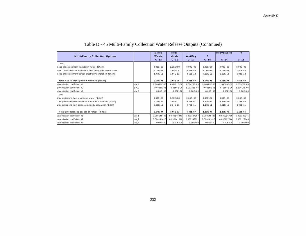
Appendix D
232
Table D - 45 Multi-Family Collection Water Release Outputs (Continued)
M ixed Resi- Recyclables 0
M u lti-Fam ily Collection Options Waste duals W e t/Dry 0
C_13 C_16 C_17 C_18 C_14 C_15
Lead
Lead emissions from washdown water (lb/ton) 0.00E+00 0.00E+00 0.00E+00 0.00E+00 0.00E+00 0.00E+00
Lead precombustion emissions from fuel production (lb/ton) 2.00E-08 2.08E-08 4.33E-08 1.04E-08 8.01E-08 7.60E-08
Lead emissions from garage electricity generation (lb/ton) 1.47E-12 1.56E-12 3.18E-12 7.82E-13 6.63E-12 6.01E-12
total lead releases per ton of refuse (lb/ton) 2.00E-08 2.08E-08 4.33E-08 1.04E-08 8.01E-08 7.60E-08
pb emission coefficient #1 pb_1 9.98471E-06 9.98471E-06 1.00429E-05 9.98471E-06 1.54606E-05 1.53576E-05
pb emission coefficient #2 pb_2 9.6556E-06 9.6556E-06 1.00241E-05 9.6556E-06 8.71665E-06 8.39617E-06
pb emission coefficient #3 pb_3 0.00E+00 0.00E+00 0.00E+00 0.00E+00 0.00E+00 0.00E+00
Zinc
Zinc emissions from washdown water (lb/ton) 0.00E+00 0.00E+00 0.00E+00 0.00E+00 0.00E+00 0.00E+00
Zinc precombustion emissions from fuel production (lb/ton) 2.94E-07 3.05E-07 6.36E-07 1.52E-07 1.17E-06 1.11E-06
Zinc emissions from garage electricity generation (lb/ton) 2.20E-11 2.34E-11 4.76E-11 1.17E-11 9.91E-11 8.99E-11
Total zinc releases per ton of refuse (lb/ton) 2.94E-07 3.05E-07 6.36E-07 1.52E-07 1.17E-06 1.12E-06
zn emission coefficient #1 zn_1 0.000146443 0.000146443 0.000147297 0.000146443 0.000226755 0.000225245
zn emission coefficient #2 zn_2 0.000141616 0.000141616 0.000147021 0.000141616 0.000127844 0.000123144
zn emission coefficient #3 zn_3 0.00E+00 0.00E+00 0.00E+00 0.00E+00 0.00E+00 0.00E+00

Appendix D
233
Table D - 46 Multi-Family Collection Solid Waste Outputs (Continued)
M ixed Resi- Recyclables 0
M u lti-Fam ily Collection Options Waste duals W e t/Dry 0
C_13 C_16 C_17 C_18 C_14 C_15
SOLID WASTE
Solid Waste #1
SW#1 precombustion emissions from fuel production (lb/ton) 1.10E-01 1.14E-01 2.38E-01 5.71E-02 4.40E-01 4.18E-01
SW#1 emissions from garage electricity generation (lb/ton) 4.27E-03 4.54E-03 9.23E-03 2.27E-03 1.92E-02 1.74E-02
total SW#1 generation per ton of refuse (lb/ton) 1.14E-01 1.19E-01 2.47E-01 5.93E-02 4.59E-01 4.35E-01
SW1 emission coefficient #1 SW1_1 5.84E+01 5.84E+01 5.88E+01 5.84E+01 9.13E+01 9.07E+01
SW1 emission coefficient #2 SW1_2 5.49E+01 5.49E+01 5.71E+01 5.49E+01 4.97E+01 4.77E+01
Solid Waste #2
SW #2 precombustion emissions from fuel production (lb/ton) 0.00E+00 0.00E+00 0.00E+00 0.00E+00 0.00E+00 0.00E+00
SW #2 emissions from garage electricity generation (lb/ton) 0.00E+00 0.00E+00 0.00E+00 0.00E+00 0.00E+00 0.00E+00
total SW #2 generation per ton of refuse (lb/ton) 0.00E+00 0.00E+00 0.00E+00 0.00E+00 0.00E+00 0.00E+00
SW2 emission coefficient #2 SW2_2 0.00E+00 0.00E+00 0.00E+00 0.00E+00 0.00E+00 0.00E+00
Solid Waste #3
SW #3 precombustion emissions from fuel production (lb/ton) 0.00E+00 0.00E+00 0.00E+00 0.00E+00 0.00E+00 0.00E+00
SW #3 emissions from garage electricity generation (lb/ton) 0.00E+00 0.00E+00 0.00E+00 0.00E+00 0.00E+00 0.00E+00
total SW #3 generation per ton of refuse (lb/ton) 0.00E+00 0.00E+00 0.00E+00 0.00E+00 0.00E+00 0.00E+00
SW3 emission coefficient #1 SW3_1 0.00E+00 0.00E+00 0.00E+00 0.00E+00 0.00E+00 0.00E+00
SW3 emission coefficient #2 SW3_2 0.00E+00 0.00E+00 0.00E+00 0.00E+00 0.00E+00 0.00E+00
Solid Waste #4
SW #4 precombustion emissions from fuel production (lb/ton) 0.00E+00 0.00E+00 0.00E+00 0.00E+00 0.00E+00 0.00E+00
SW #4 emissions from garage electricity generation (lb/ton) 0.00E+00 0.00E+00 0.00E+00 0.00E+00 0.00E+00 0.00E+00
total SW #4 generation per ton of refuse (lb/ton) 0.00E+00 0.00E+00 0.00E+00 0.00E+00 0.00E+00 0.00E+00
SW4 emission coefficient #1 SW4_1 0.00E+00 0.00E+00 0.00E+00 0.00E+00 0.00E+00 0.00E+00
SW4 emission coefficient #2 SW4_2 0.00E+00 0.00E+00 0.00E+00 0.00E+00 0.00E+00 0.00E+00
Solid Waste #5
SW #5 precombustion emissions from fuel production (lb/ton) 0.00E+00 0.00E+00 0.00E+00 0.00E+00 0.00E+00 0.00E+00
SW #5 emissions from garage electricity generation (lb/ton) 0.00E+00 0.00E+00 0.00E+00 0.00E+00 0.00E+00 0.00E+00
total SW #5 generation per ton of refuse (lb/ton) 0.00E+00 0.00E+00 0.00E+00 0.00E+00 0.00E+00 0.00E+00
SW5 emission coefficient #1 SW5_1 0.00E+00 0.00E+00 0.00E+00 0.00E+00 0.00E+00 0.00E+00
SW5 emission coefficient #2 SW5_2 0.00E+00 0.00E+00 0.00E+00 0.00E+00 0.00E+00 0.00E+00

Appendix D
234
Table D - 47 Commercial Collection Outputs
Recyc- M S W /
Commercial Collection Options labels Residuals
C_19 C_20
COLLECTION COSTS
Breakdown of capital costs capital cost per vehicle ($/vehicle-year) Ct 9,641 25,845
number of collection vehicles (vehicles) Nt 1.63 1.65
12.28
Breakdown of operating costs labor cost per vehicle ($/vehicle-year) Cw 40,196 69,170
O&M cost per vehicle ($/vehicle-year) Cvo 30,822 29,376
other expenses per vehicle ($/vehicle-year) Coe 8,083 16,166
Annual operating cost ($/year) C_op 88,593 128,477
Total annual cost ($/year) -- capital + operating C_ann 161,339 258,360
Total annual cost per location ($/location-year) C_location 1,613.39 2,583.60
Cost per ton of refuse collected ($/ton) C_ton 181.01 50.61
Total annual cost per vehicle ($/vehicle-year) C_vehicle 99,198 156,907
cost coefficient #1 cc_1 87,511.77 51,727.89
cost coefficient #2 cc_2 8,064.65 13,305.01
Table D - 48 Commercial Collection Outputs (Continued)
Recyc- MSW /
Commercial Collection Options labels ResidualsC_19 C_20
Calculations for collection vehicle activities
locations per trip Ht 12.28 8.99
travel time between collection locations (min/stop) Tbet 1.50 1.50
travel time from collection route to disposal facility (min/trip) Trf 20.00 20.00
travel time from garage to first collection route (min/day-vehicle) Tgr 20.00 20.00
travel time from disposal facility to garage (min/day-vehicle) Tfg 20.00 20.00
time per trip (min/trip) -- collection+travel+unload time Tc 199.71 111.92
trips per day per vehicle (trips/day-vehicle) RD 1.50 2.70
daily weight of refuse collected per vehicle (tons/day) RefD 2.10 11.89
number of collection stops per day (stops/vehicle-day) SD 18.45 24.29
Collection vehicle activity timestravel time from garage to first collection route (min/day-vehicle) Tgr 20.00 20.00
loading time at collection stops (min/day-vehicle) LD 184.45 121.46
travel time between collection stops (min/day-vehicle) Tb 25.41 32.39
travel time between disposal facility and route (min/day-vehicle) F_R 70.09 118.11
unloading time at disposal facility (min/day-vehicle) UD 40.04 48.04
lunch time (min/day-vehicle) F1_ 30.00 30.00
break time (min/day-vehicle) F2_ 30.00 30.00
travel time from disposal facility to garage (min/day-vehicle) Tfg 20.00 20.00
actual working time (min/day-vehicle) 420.00 420.00
service hours per day (hours/day-vehicle) ShD 6.00 6.00
Daily m iles traveled per collection vehicle
from garage to first collection route (miles/day) Dgr 11.67 11.67
between collection stops (miles/day) Db 4.24 5.40
between disposal facility and route (miles/day) DF_R 35.04 59.05
from disposal facility to garage (miles/day) Dfg 11.67 11.67
total (miles/day) Mi 62.61 87.79
Daily fuel usage per collection vehiclefrom garage to first collection route (gallons/day) 2.33 2.33
loading at collection stops (gallons/day) 3.07 2.02
between collection stops (gallons/day) 2.12 2.70
between disposal facility and route (gallons/day) 7.01 11.81
unloading at disposal facility (gallons/day) 0.67 0.80
from disposal facility to garage (gallons/day) 2.33 2.33
total (gallons/day) FuelD 17.54 22.00
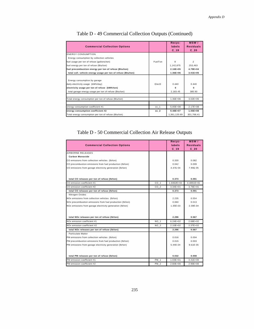
Appendix D
235
Table D - 49 Commercial Collection Outputs (Continued)
Recyc- M S W /
Commercial Collection Options labels Residuals
C_19 C_20
ENERGY CONSUMPTION
Energy consumption by collection vehicles
fuel usage per ton of refuse (gallons/ton) FuelTon 8 2
fuel energy per ton of refuse (Btu/ton) 1,142,875 253,463
fuel precombustion energy per ton of refuse (Btu/ton) 2.16E+05 4.79E+04
total coll. vehicle energy usage per ton of refuse (Btu/ton) 1.36E+06 3.01E+05
Energy consumption by garage
daily electricity usage (kWh/day) ElecD 0.440 0.440
electricity usage per ton of refuse (kWh/ton) 0 0
total garage energy usage per ton of refuse (Btu/ton) 2,183.45 385.93
Total energy consumption per ton of refuse (Btu/ton) 1.36E+06 3.02E+05
energy consumption coefficient #1 ec_1 5.05E+08 2.17E+08
energy consumption coefficient #2 ec_2 9.48E+07 1.05E+08
Total energy consumption per ton of refuse (Btu/ton) 1,361,120.69 301,766.41
Table D - 50 Commercial Collection Air Release Outputs
Recyc- M S W /
Commercial Collection Options labels Residuals
C_19 C_20
AIRBORNE RELEASES
Carbon Monoxide
CO emissions from collection vehicles (lb/ton) 0.330 0.082
CO precombustion emissions from fuel production (lb/ton) 0.042 0.009
CO emissions from garage electricity generation (lb/ton) 4.47E-04 7.90E-05
total CO releases per ton of refuse (lb/ton) 0.373 0.091
CO emission coefficient #1 CO_1 1.0462E+02 4.4851E+01
CO emission coefficient #2 CO_2 3.34E+01 3.76E+01
total CO releases per ton of refuse (lb/ton) 0.373 0.091
Nitrogen Oxides
NOx emissions from collection vehicles (lb/ton) 2.235 0.554
NOx precombustion emissions from fuel production (lb/ton) 0.060 0.013
NOx emissions from garage electricity generation (lb/ton) 1.35E-03 2.39E-04
total NOx releases per ton of refuse (lb/ton) 2.296 0.567
NOx emission coefficient #1 NO_1 6.24E+02 2.68E+02
NOx emission coefficient #2 NO_2 2.10E+02 2.37E+02
total NOx releases per ton of refuse (lb/ton) 2.296 0.567
Particulate Matter
PM emissions from collection vehicles (lb/ton) 0.016 0.004
PM precombustion emissions from fuel production (lb/ton) 0.015 0.003
PM emissions from garage electricity generation (lb/ton) 5.44E-04 9.61E-05
total PM releases per ton of refuse (lb/ton) 0.032 0.008
PM emission coefficient #1 PM_1 1.03E+01 4.41E+00
PM emission coefficient #2 PM_2 2.60E+00 2.90E+00

Appendix D
236
Table D - 51 Commercial Collection Air Release Outputs (Continued)
Recyc- M S W /
Commercial Col lect ion Options labels Residuals
C_19 C_20
PM10
PM10 emissions from collection vehicles (lb/ton) 0.000 0.000
PM10 precombustion emissions from fuel production (lb/ton) 0.000 0.000
PM10 emissions from garage electricity generation (lb/ton) 0.00E+00 0.00E+00
total PM10 releases per ton of refuse (lb/ton) 0.000 0.000
PM10 emission coefficient #1 PM10_1 0.00E+00 0.00E+00
PM10 emission coefficient #2 PM10_2 0.00E+00 0.00E+00
total PM10 releases per ton of refuse (lb/ton) 0.000 0.000
Fossil CO2
CO2-fossil emissions from collection vehicles (lb/ton) 0.000 0.000
CO2-fossil precombustion emissions from fuel production (lb/ton) 29.982 6.649
CO2-fossil emissions from garage electricity generation (lb/ton) 3.11E-01 5.50E-02
total CO2-fossil releases per ton of refuse (lb/ton) 30.293 6.704
CO2-fossil emission coefficient #1 CO2f_1 1.13E+04 4.84E+03
CO2-fossil emission coefficient #2 CO2f_2 2.10E+03 2.33E+03
total CO2-fossil releases per ton of refuse (lb/ton) 30.293 6.704
Biomass CO2
CO2-biomass emissions from collection vehicles (lb/ton) 0.000 0.000
CO2-biomass precombustion emissions from fuel production (lb/ton) 0.000 0.000
CO2-biomass emissions from garage electricity generation (lb/ton) 0.00E+00 0.00E+00
total CO2-biomass releases per ton of refuse (lb/ton) 0.00E+00 0.00E+00
CO2-biomass emission coefficient #1 CO2bm_1 0.00E+00 0.00E+00
CO2-biomass emission coefficient #2 CO2bm_2 0.00E+00 0.00E+00
total CO2-biomass releases per ton of refuse (lb/ton) 0.00E+00 0.00E+00
Table D - 52 Commercial Collection Air Release Outputs (Continued)
Recyc- M S W /
Commercial Collection Options labels Residuals
C_19 C_20
Sulfur Oxides
SOx emissions from collection vehicles (lb/ton) 0.000 0.000
SOx precombustion emissions from fuel production (lb/ton) 0.073 0.016
SOx emissions from garage electricity generation (lb/ton) 2.86E-03 5.06E-04
total SOx releases per ton refuse ( lb/ton) 0.076 0.017
SOx emission coefficient #1 SOx_1 2.86E+01 1.22E+01
SOx emission coefficient #2 SOx_2 5.24E+00 5.80E+00
total SOx releases per ton refuse ( lb/ton) 0.076 0.017
Hydrocarbons (less methane)
HC emissions from collection vehicles (lb/ton) 0.040 0.010
HC precombustion emissions from collection vehicles (lb/ton) 0.563 0.125
HC emissions from garage electricity generation (lb/ton) 2.14E-04 3.78E-05
total HC releases per ton of refuse ( lb/ton) 0.603 0.135
HC emission coefficient #1 HC_1 2.20E+02 9.45E+01
HC emission coefficient #2 HC_2 4.29E+01 4.76E+01
Methane
CH4 emissions from collection vehicles (lb/ton) 0.000 0.000
CH4 precombustion emissions from fuel production (lb/ton) 4.17E-04 9.25E-05
CH4 emissions from garage electricity generation (lb/ton) 2.06E-06 3.64E-07
total CH4 releases per ton of refuse ( lb/ton) 0.000 0.000
CH4 emission coefficient #1 CH4_1 1.56E-01 6.69E-02
CH4 emission coefficient #2 CH4_2 2.91E-02 3.23E-02

Appendix D
237
Table D - 53 Commercial Collection Air Release Outputs (Continued)
Recyc- M S W /
Commercial Collection Options labels Residuals
C_19 C_20
Lead
Lead emissions from collection vehicles (lb/ton) 0.000 0.000
Lead precombustion emissions from fuel production (lb/ton) 9.18E-08 2.04E-08
Lead emissions from garage electricity generation (lb/ton) 1.03E-11 1.82E-12
total lead releases per ton of refuse (lb/ton) 9.18E-08 2.04E-08
Pb emission coefficient #1 Pb_a_1 1.03E-03 3.87E-04
PB emission coefficient #2 Pb_a_2 9.82E-05 1.03E-04
Ammonia
Ammonia emissions from collection vehicles (lb/ton) 0.000 0.000
Ammonia precombustion emissions from fuel production (lb/ton) 3.25E-04 7.22E-05
Ammonia emissions from garage electricity generation (lb/ton) 3.69E-08 6.51E-09
total ammonia releases per ton of refuse ( lb/ton) 3.25E-04 7.22E-05
NH3 emission coefficient #1 NH3_1 1.03E-03 3.87E-04
NH3 emission coefficient #2 NH3_2 9.82E-05 1.03E-04
Hydrochloric Acid
HCl emissions from collection vehicles (lb/ton) 0.000 0.000
HCl precombustion emissions from fuel production (lb/ton) 1.00E-05 2.22E-06
HCl emissions from garage electricity generation (lb/ton) 1.11E-09 1.97E-10
total HCl releases per ton of refuse (lb/ton) 1.00E-05 2.22E-06
HCl emission coefficient #1 HCl_1 3.71E-03 1.60E-03
HCl emission coefficient #2 HCl_2 6.97E-04 7.72E-04
Table D - 54 Commercial Collection Air Release Outputs (Continued)
Recyc- M S W /
Commercial Collection Options labels Residuals
C_19 C_20
Greenhouse Gas Equivalence
Carbon dioxide (fossil fuel) 30.29 6.70
Carbon dioxide (biomass) 0.00 0.00
Methane 0.03 0.01
Nitrous oxide 619.88 153.17
Other hydrocarbons 0.00 0.00
total greenhouse gas equivalence per ton of refuse 650.20 159.88
GHE emission coefficient #1 GHE_1 1.80E+05 7.71E+04
GHE emission coefficient #2 GHE_2 5.89E+04 6.63E+04
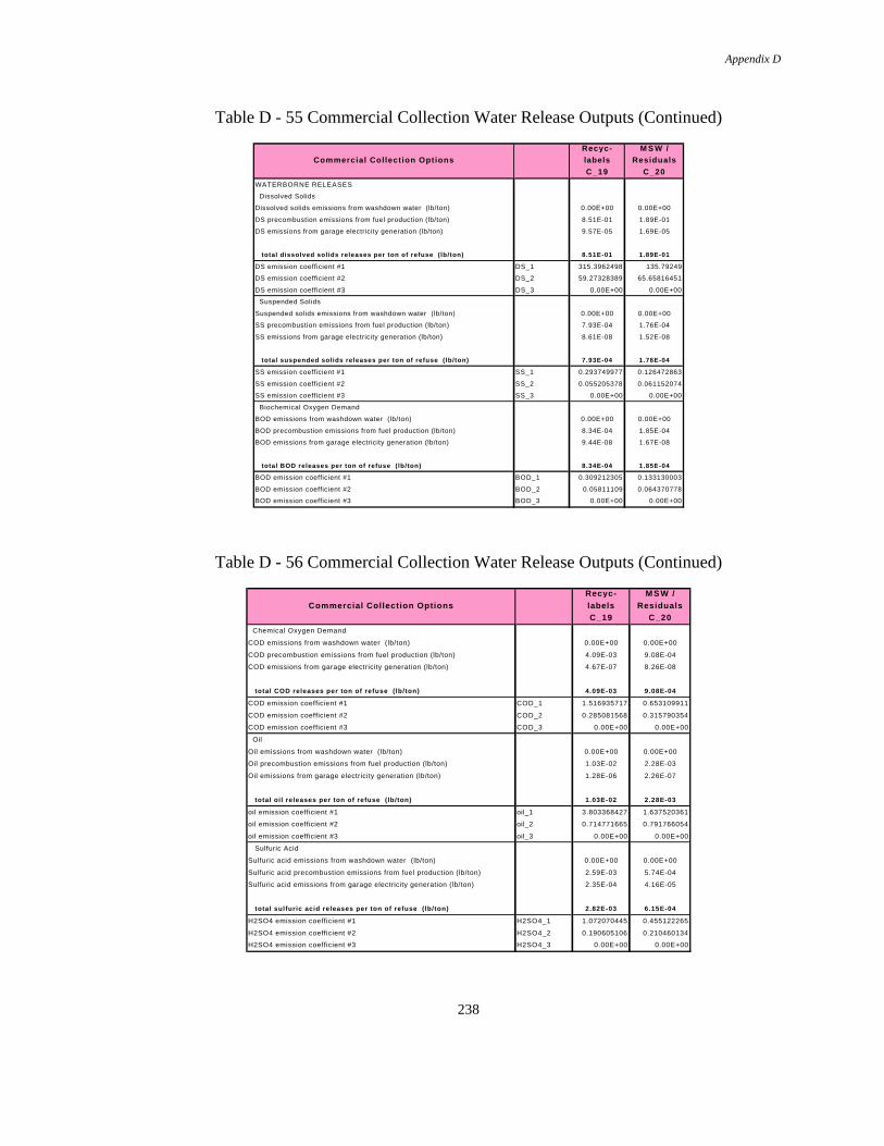
Appendix D
238
Table D - 55 Commercial Collection Water Release Outputs (Continued)
Recyc- M S W /
Commercial Collection Options labels Residuals
C_19 C_20
WATERBORNE RELEASES
Dissolved Solids
Dissolved solids emissions from washdown water (lb/ton) 0.00E+00 0.00E+00
DS precombustion emissions from fuel production (lb/ton) 8.51E-01 1.89E-01
DS emissions from garage electricity generation (lb/ton) 9.57E-05 1.69E-05
total dissolved solids releases per ton of refuse (lb/ton) 8.51E-01 1.89E-01
DS emission coefficient #1 DS_1 315.3962498 135.79249
DS emission coefficient #2 DS_2 59.27328389 65.65816451
DS emission coefficient #3 DS_3 0.00E+00 0.00E+00
Suspended Solids
Suspended solids emissions from washdown water (lb/ton) 0.00E+00 0.00E+00
SS precombustion emissions from fuel production (lb/ton) 7.93E-04 1.76E-04
SS emissions from garage electricity generation (lb/ton) 8.61E-08 1.52E-08
total suspended solids releases per ton of refuse (lb/ton) 7.93E-04 1.76E-04
SS emission coefficient #1 SS_1 0.293749977 0.126472863
SS emission coefficient #2 SS_2 0.055205378 0.061152074
SS emission coefficient #3 SS_3 0.00E+00 0.00E+00
Biochemical Oxygen Demand
BOD emissions from washdown water (lb/ton) 0.00E+00 0.00E+00
BOD precombustion emissions from fuel production (lb/ton) 8.34E-04 1.85E-04
BOD emissions from garage electricity generation (lb/ton) 9.44E-08 1.67E-08
total BOD releases per ton of refuse (lb/ton) 8.34E-04 1.85E-04
BOD emission coefficient #1 BOD_1 0.309212305 0.133130003
BOD emission coefficient #2 BOD_2 0.05811109 0.064370778
BOD emission coefficient #3 BOD_3 0.00E+00 0.00E+00
Table D - 56 Commercial Collection Water Release Outputs (Continued)
Recyc- M S W /
Commercial Collection Options labels Residuals
C_19 C_20
Chemical Oxygen Demand
COD emissions from washdown water (lb/ton) 0.00E+00 0.00E+00
COD precombustion emissions from fuel production (lb/ton) 4.09E-03 9.08E-04
COD emissions from garage electricity generation (lb/ton) 4.67E-07 8.26E-08
total COD releases per ton of refuse (lb/ton) 4.09E-03 9.08E-04
COD emission coefficient #1 COD_1 1.516935717 0.653109911
COD emission coefficient #2 COD_2 0.285081568 0.315790354
COD emission coefficient #3 COD_3 0.00E+00 0.00E+00
Oil
Oil emissions from washdown water (lb/ton) 0.00E+00 0.00E+00
Oil precombustion emissions from fuel production (lb/ton) 1.03E-02 2.28E-03
Oil emissions from garage electricity generation (lb/ton) 1.28E-06 2.26E-07
total oil releases per ton of refuse (lb/ton) 1.03E-02 2.28E-03
oil emission coefficient #1 oil_1 3.803368427 1.637520361
oil emission coefficient #2 oil_2 0.714771665 0.791766054
oil emission coefficient #3 oil_3 0.00E+00 0.00E+00
Sulfuric Acid
Sulfuric acid emissions from washdown water (lb/ton) 0.00E+00 0.00E+00
Sulfuric acid precombustion emissions from fuel production (lb/ton) 2.59E-03 5.74E-04
Sulfuric acid emissions from garage electricity generation (lb/ton) 2.35E-04 4.16E-05
total sulfuric acid releases per ton of refuse (lb/ton) 2.82E-03 6.15E-04
H2SO4 emission coefficient #1 H2SO4_1 1.072070445 0.455122265
H2SO4 emission coefficient #2 H2SO4_2 0.190605106 0.210460134
H2SO4 emission coefficient #3 H2SO4_3 0.00E+00 0.00E+00

Appendix D
239
Table D - 57 Commercial Collection Water Release Outputs (Continued)
Recyc- M S W /
Commercial Collection Options labels Residuals
C_19 C_20
Iron
Iron emissions from washdown water (lb/ton) 0.00E+00 0.00E+00
Iron precombustion emissions from fuel production (lb/ton) 6.76E-04 1.50E-04
Iron emissions from garage electricity generation (lb/ton) 5.85E-05 1.03E-05
total iron releases per ton of refuse (lb/ton) 7.34E-04 1.60E-04
fe emission coefficient #1 fe_1 0.278698443 0.118387201
fe emission coefficient #2 fe_2 0.049672115 0.0548544
fe emission coefficient #3 fe_3 0.00E+00 0.00E+00
Ammonia
Ammonia emissions from washdown water (lb/ton) 0.00E+00 0.00E+00
Ammonia precombustion emissions from fuel production (lb/ton) 1.17E-04 2.59E-05
Ammonia emissions from garage electricity generation (lb/ton) 1.29E-08 2.27E-09
total ammonia releases per ton of refuse ( lb/ton) 1.17E-04 2.59E-05
NH4 emission coefficient #1 NH4_1 0.043289555 0.018638138
NH4 emission coefficient #2 NH4_2 0.008135537 0.009011893
NH4 emission coefficient #3 NH4_3 0.00E+00 0.00E+00
Copper
Copper emissions from washdown water (lb/ton) 0.00E+00 0.00E+00
Copper precombustion emissions from fuel production (lb/ton) 0.00E+00 0.00E+00
Copper emissions from garage electricity generation (lb/ton) 0.00E+00 0.00E+00
total copper releases per ton of refuse (lb/ton) 0.00E+00 0.00E+00
cu emission coefficient #1 cu_1 0 0
cu emission coefficient #2 cu_2 0 0
cu emission coefficient #3 cu_3 0.00E+00 0.00E+00
Table D - 58 Commercial Collection Water Release Outputs (Continued)
Recyc- M S W /
Commercial Collection Options labels Residuals
C_19 C_20
Cadmium
Cadmium emissions from washdown water (lb/ton) 0.00E+00 0.00E+00
Cadmium precombustion emissions from fuel production (lb/ton) 0.00E+00 0.00E+00
Cadmium emissions from garage electricity generation (lb/ton) 0.00E+00 0.00E+00
total cadmium releases per ton of refuse ( lb/ton) 0.00E+00 0.00E+00
cd emission coefficient #1 cd_1 0 0
cd emission coefficient #2 cd_2 0 0
cd emission coefficient #3 cd_3 0.00E+00 0.00E+00
Arsenic
Arsenic emissions from washdown water (lb/ton) 0.00E+00 0.00E+00
Arsenic precombustion emissions from fuel production (lb/ton) 0.00E+00 0.00E+00
Arsenic emissions from garage electricity generation (lb/ton) 0.00E+00 0.00E+00
total arsenic releases per ton of refuse (lb/ton) 0.00E+00 0.00E+00
as emission coefficient #1 as_1 0 0
as emission coefficient #2 as_2 0 0
as emission coefficient #3 as_3 0.00E+00 0.00E+00
Mercury
Mercury emissions from washdown water (lb/ton) 0.00E+00 0.00E+00
Mercury precombustion emissions from fuel production (lb/ton) 0.00E+00 0.00E+00
Mercury emissions from garage electricity generation (lb/ton) 0.00E+00 0.00E+00
total mercury releases per ton of refuse ( lb/ton) 0.00E+00 0.00E+00
hg emission coefficient #1 hg_1 0 0
hg emission coefficient #2 hg_2 0 0
hg emission coefficient #3 hg_3 0.00E+00 0.00E+00
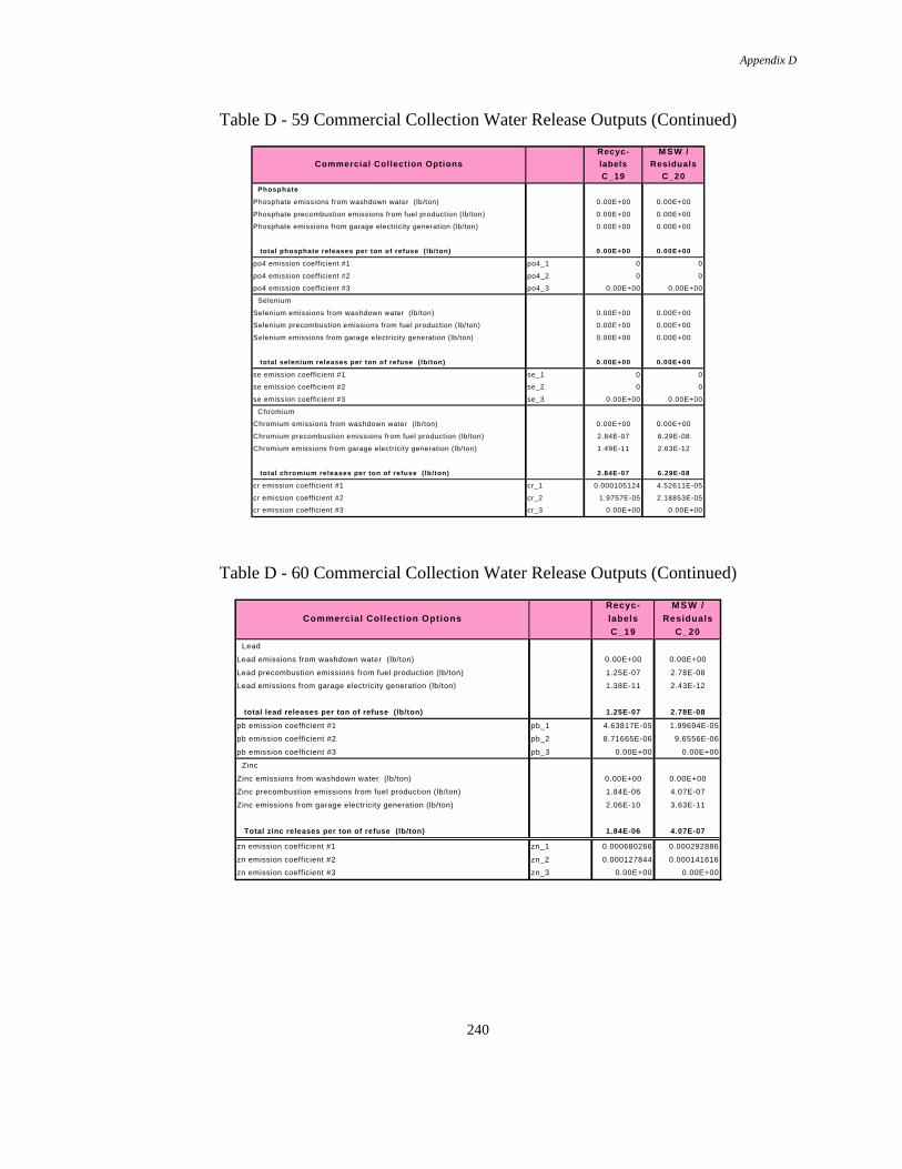
Appendix D
240
Table D - 59 Commercial Collection Water Release Outputs (Continued)
Recyc- M S W /
Commercial Collection Options labels Residuals
C_19 C_20
Phosphate
Phosphate emissions from washdown water (lb/ton) 0.00E+00 0.00E+00
Phosphate precombustion emissions from fuel production (lb/ton) 0.00E+00 0.00E+00
Phosphate emissions from garage electricity generation (lb/ton) 0.00E+00 0.00E+00
total phosphate releases per ton of refuse ( lb/ton) 0.00E+00 0.00E+00
po4 emission coefficient #1 po4_1 0 0
po4 emission coefficient #2 po4_2 0 0
po4 emission coefficient #3 po4_3 0.00E+00 0.00E+00
Selenium
Selenium emissions from washdown water (lb/ton) 0.00E+00 0.00E+00
Selenium precombustion emissions from fuel production (lb/ton) 0.00E+00 0.00E+00
Selenium emissions from garage electricity generation (lb/ton) 0.00E+00 0.00E+00
total selenium releases per ton of refuse ( lb/ton) 0.00E+00 0.00E+00
se emission coefficient #1 se_1 0 0
se emission coefficient #2 se_2 0 0
se emission coefficient #3 se_3 0.00E+00 0.00E+00
Chromium
Chromium emissions from washdown water (lb/ton) 0.00E+00 0.00E+00
Chromium precombustion emissions from fuel production (lb/ton) 2.84E-07 6.29E-08
Chromium emissions from garage electricity generation (lb/ton) 1.49E-11 2.63E-12
total chromium releases per ton of refuse ( lb/ton) 2.84E-07 6.29E-08
cr emission coefficient #1 cr_1 0.000105124 4.52611E-05
cr emission coefficient #2 cr_2 1.9757E-05 2.18853E-05
cr emission coefficient #3 cr_3 0.00E+00 0.00E+00
Table D - 60 Commercial Collection Water Release Outputs (Continued)
Recyc- M S W /
Commercial Collection Options labels Residuals
C_19 C_20
Lead
Lead emissions from washdown water (lb/ton) 0.00E+00 0.00E+00
Lead precombustion emissions from fuel production (lb/ton) 1.25E-07 2.78E-08
Lead emissions from garage electricity generation (lb/ton) 1.38E-11 2.43E-12
total lead releases per ton of refuse (lb/ton) 1.25E-07 2.78E-08
pb emission coefficient #1 pb_1 4.63817E-05 1.99694E-05
pb emission coefficient #2 pb_2 8.71665E-06 9.6556E-06
pb emission coefficient #3 pb_3 0.00E+00 0.00E+00
Zinc
Zinc emissions from washdown water (lb/ton) 0.00E+00 0.00E+00
Zinc precombustion emissions from fuel production (lb/ton) 1.84E-06 4.07E-07
Zinc emissions from garage electricity generation (lb/ton) 2.06E-10 3.63E-11
Total zinc releases per ton of refuse (lb/ton) 1.84E-06 4.07E-07
zn emission coefficient #1 zn_1 0.000680266 0.000292886
zn emission coefficient #2 zn_2 0.000127844 0.000141616
zn emission coefficient #3 zn_3 0.00E+00 0.00E+00

Appendix D
241
Table D - 61 Commercial Collection Solid Waste Outputs (Continued)
Recyc- M S W /
Commercial Collection Options labels Residuals
C_19 C_20
SOLID WASTE
Solid Waste #1
SW#1 precombustion emissions from fuel production (lb/ton) 6.87E-01 1.52E-01
SW#1 emissions from garage electricity generation (lb/ton) 3.99E-02 7.05E-03
total SW#1 generation per ton of refuse (lb/ton) 7.27E-01 1.60E-01
SW1 emission coefficient #1 SW1_1 2.74E+02 1.17E+02
SW1 emission coefficient #2 SW1_2 4.97E+01 5.49E+01
Solid Waste #2
SW #2 precombustion emissions from fuel production (lb/ton) 0.00E+00 0.00E+00
SW #2 emissions from garage electricity generation (lb/ton) 0.00E+00 0.00E+00
total SW #2 generation per ton of refuse (lb/ton) 0.00E+00 0.00E+00
SW2 emission coefficient #2 SW2_2 0.00E+00 0.00E+00
Solid Waste #3
SW #3 precombustion emissions from fuel production (lb/ton) 0.00E+00 0.00E+00
SW #3 emissions from garage electricity generation (lb/ton) 0.00E+00 0.00E+00
total SW #3 generation per ton of refuse (lb/ton) 0.00E+00 0.00E+00
SW3 emission coefficient #1 SW3_1 0.00E+00 0.00E+00
SW3 emission coefficient #2 SW3_2 0.00E+00 0.00E+00
Solid Waste #4
SW #4 precombustion emissions from fuel production (lb/ton) 0.00E+00 0.00E+00
SW #4 emissions from garage electricity generation (lb/ton) 0.00E+00 0.00E+00
total SW #4 generation per ton of refuse (lb/ton) 0.00E+00 0.00E+00
SW4 emission coefficient #1 SW4_1 0.00E+00 0.00E+00
SW4 emission coefficient #2 SW4_2 0.00E+00 0.00E+00
Solid Waste #5
SW #5 precombustion emissions from fuel production (lb/ton) 0.00E+00 0.00E+00
SW #5 emissions from garage electricity generation (lb/ton) 0.00E+00 0.00E+00
total SW #5 generation per ton of refuse (lb/ton) 0.00E+00 0.00E+00
SW5 emission coefficient #1 SW5_1 0.00E+00 0.00E+00
SW5 emission coefficient #2 SW5_2 0.00E+00 0.00E+00

Appendix E
242
APPENDIX E
COEFFICIENTS FOR OPTIMIZATION
Appendix E
243
The Collection Preprocessor provides sets of coefficients for selected collection cost,consumption and release rates. The coefficient sets effectively condense all of theCollection Preprocessor calculations associated with the selected rate into two or threecoefficients except for calculations involving waste generation rates and densities. Wastegeneration rates and, in some cases, densities are functions of variables such as per capitawaste generation rates and residential/multi-family population figures. Operating instand-alone mode as presented in this report, the Collection Preprocessor worksheetobtains waste generation rates from the Generation Preprocessor that apply to the entirecommunity. By contrast, the Optimization Model can use the coefficients to evaluatecollection costs and other optimization parameters for fractions of the community. TheCollection Preprocessor can model the results of such an optimization by assigning valuesother than 100% or 0% to the fraction of the community served by a particular collectionoption using the option_frac variable. However, as stated earlier in this document, it isimportant to understand the limitations of the results of a stand alone analysis using thecollection preprocessor. Use of the process model in this mode should be attempted onlyby a user that thoroughly understands the workings of the model and these limitations.

Appendix E
244
COLLECTION COST COEFFICIENTS
The collection cost per ton of waste collected for all waste collection options can beexpressed as:
avgDcc
totalGcc
tonC_
2_
_
1__ += ,
where:
cc _1 = cost coefficient #1 $ −
− −
poundhousehold week ton
cc _2 = cost coefficient #2 $ −
−
poundcubic yard ton
G total_ = total waste generation rate for all waste types (pounds per household per week)
D avg_ = average density of waste in all compartments of thecollection vehicle (pounds per cubic yard)
The equations for cost coefficients #1 and #2 vary slightly for different collection options,as shown below.
Mixed Waste, Yard Waste, Residuals, and Co-Collection Options
Cost coefficients #1 and #2 for residential waste collection options C0, C1, C5, C6,C7,and C9, multi-family waste collection options C13 and C16, and commercialcollection options C19 and C20 are defined as:
( )cc
FrCD HS
Tbet TL_ ,1 2 0001
2
7365=
××
+ ×
× ×
αα
( )cc
CD Ut Vt
Tbet Trf S_ ,2
1 22 0001
2
7365=
× ××
− + × + ×
× ×
αα
where:
( ) ( ) ( ) ( ) ( )[ ] ( ){ }α1
1 1 1 1 3657 1= + × + × × + + × + × × + × × × + + × +e bv CRF Pt a bw Wa Nw Wd WP CD c d Nw
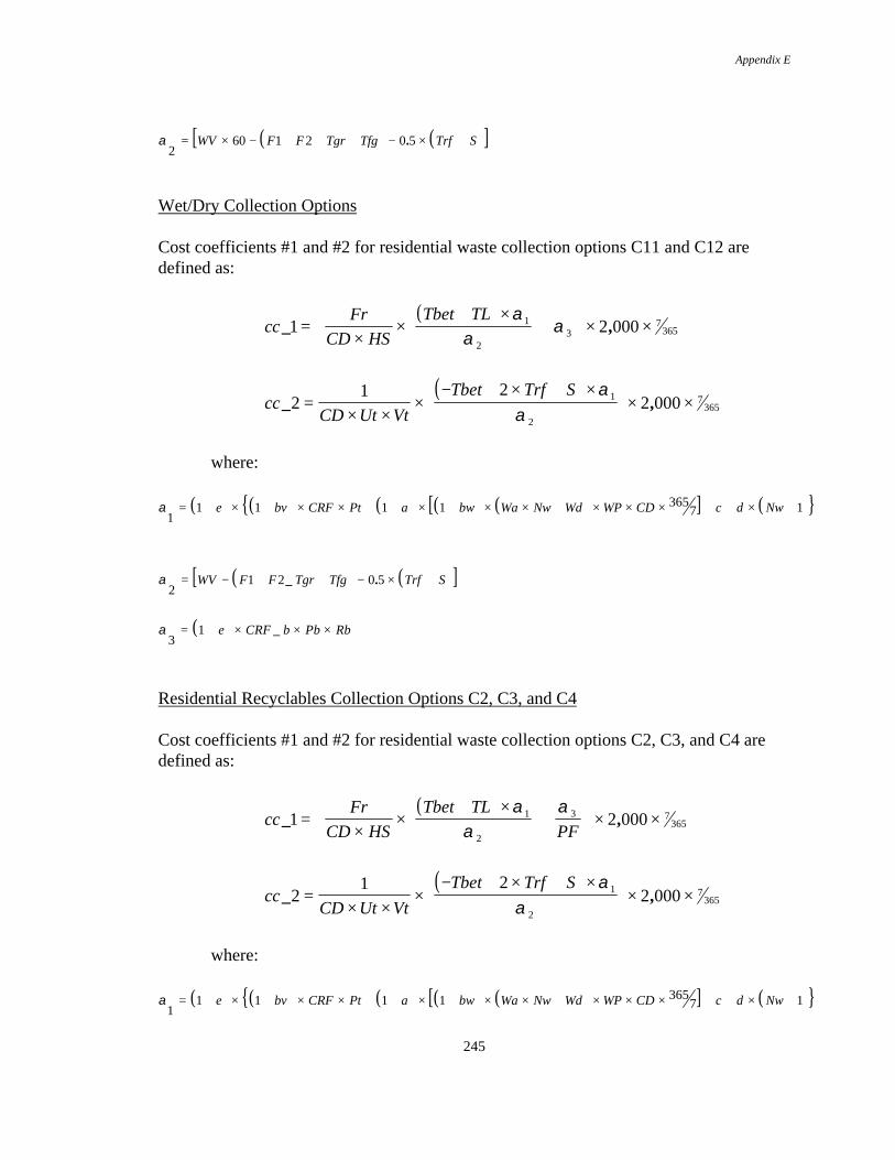
Appendix E
245
( ) ( )[ ]α2
60 1 2 0 5= × − + + + − × +WV F F Tgr Tfg Trf S.
Wet/Dry Collection Options
Cost coefficients #1 and #2 for residential waste collection options C11 and C12 aredefined as:
( )cc
FrCD HS
Tbet TL_ ,1 2 0001
23
7365=
××
+ ×
+
× ×α
αα
( )cc
CD Ut Vt
Tbet Trf S_ ,2
1 22 0001
2
7365=
× ××
− + × + ×
× ×
αα
where:
( ) ( ) ( ) ( ) ( )[ ] ( ){ }α1
1 1 1 1 3657 1= + × + × × + + × + × × + × × × + + × +e bv CRF Pt a bw Wa Nw Wd WP CD c d Nw
( ) ( )[ ]α2
1 2 0 5= − + + − × +WV F F Tgr Tfg Trf S_ .
( )α3
1= + × × ×e CRF b Pb Rb_
Residential Recyclables Collection Options C2, C3, and C4
Cost coefficients #1 and #2 for residential waste collection options C2, C3, and C4 aredefined as:
( )cc
FrCD HS
Tbet TLPF
_ ,1 2 0001
2
3 7365=
××
+ ×
+
× ×α
αα
( )cc
CD Ut Vt
Tbet Trf S_ ,2
1 22 0001
2
7365=
× ××
− + × + ×
× ×
αα
where:
( ) ( ) ( ) ( ) ( )[ ] ( ){ }α1
1 1 1 1 3657 1= + × + × × + + × + × × + × × × + + × +e bv CRF Pt a bw Wa Nw Wd WP CD c d Nw
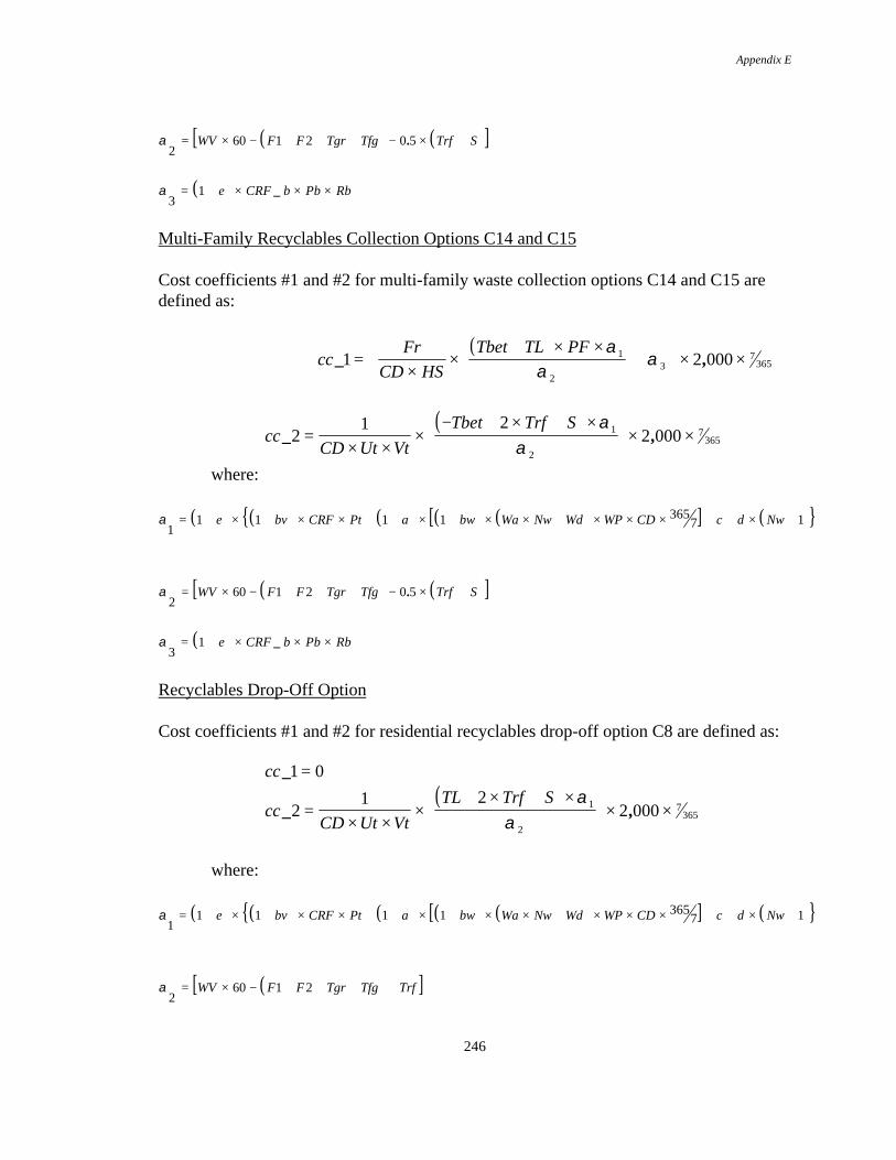
Appendix E
246
( ) ( )[ ]α2
60 1 2 0 5= × − + + + − × +WV F F Tgr Tfg Trf S.
( )α3
1= + × × ×e CRF b Pb Rb_
Multi-Family Recyclables Collection Options C14 and C15
Cost coefficients #1 and #2 for multi-family waste collection options C14 and C15 aredefined as:
( )cc
FrCD HS
Tbet TL PF_ ,1 2 0001
23
7365=
××
+ × ×
+
× ×α
αα
( )cc
CD Ut Vt
Tbet Trf S_ ,2
1 22 0001
2
7365=
× ××
− + × + ×
× ×
αα
where:
( ) ( ) ( ) ( ) ( )[ ] ( ){ }α1
1 1 1 1 3657 1= + × + × × + + × + × × + × × × + + × +e bv CRF Pt a bw Wa Nw Wd WP CD c d Nw
( ) ( )[ ]α2
60 1 2 0 5= × − + + + − × +WV F F Tgr Tfg Trf S.
( )α3
1= + × × ×e CRF b Pb Rb_
Recyclables Drop-Off Option
Cost coefficients #1 and #2 for residential recyclables drop-off option C8 are defined as:
cc _1 0=( )
ccCD Ut Vt
TL Trf S_ ,2
1 22 0001
2
7365=
× ××
+ × + ×
× ×
αα
where:
( ) ( ) ( ) ( ) ( )[ ] ( ){ }α1
1 1 1 1 3657 1= + × + × × + + × + × × + × × × + + × +e bv CRF Pt a bw Wa Nw Wd WP CD c d Nw
( )[ ]α2
60 1 2= × − + + + +WV F F Tgr Tfg Trf

Appendix E
247
Yard Waste Drop-Off Option
Cost coefficients #1 and #2 for residential yard waste drop-off option C10 are defined as:
cc _1 0=
cc _2 0=
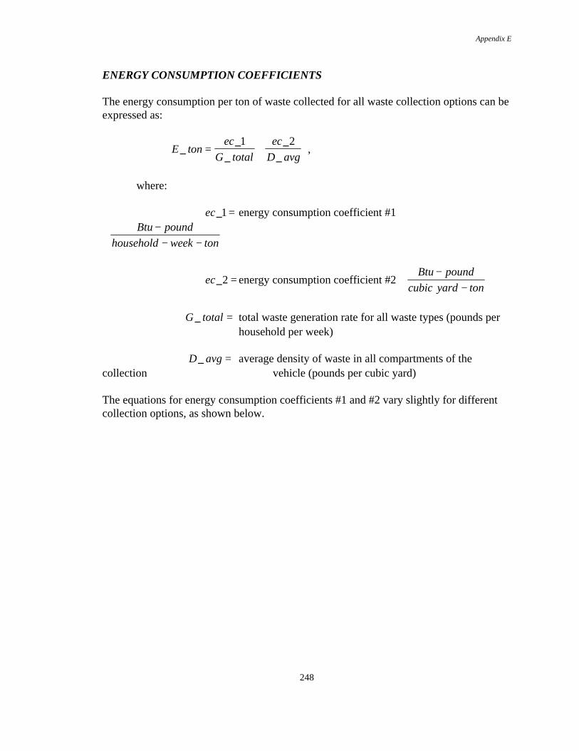
Appendix E
248
ENERGY CONSUMPTION COEFFICIENTS
The energy consumption per ton of waste collected for all waste collection options can beexpressed as:
E tonec
G totalec
D avg_
__
__
= +1 2
,
where:
ec _1 = energy consumption coefficient #1Btu pound
household week ton−
− −
ec _2 = energy consumption coefficient #2 Btu pound
cubic yard ton−
−
G total_ = total waste generation rate for all waste types (pounds per household per week)
D avg_ = average density of waste in all compartments of thecollection vehicle (pounds per cubic yard)
The equations for energy consumption coefficients #1 and #2 vary slightly for differentcollection options, as shown below.
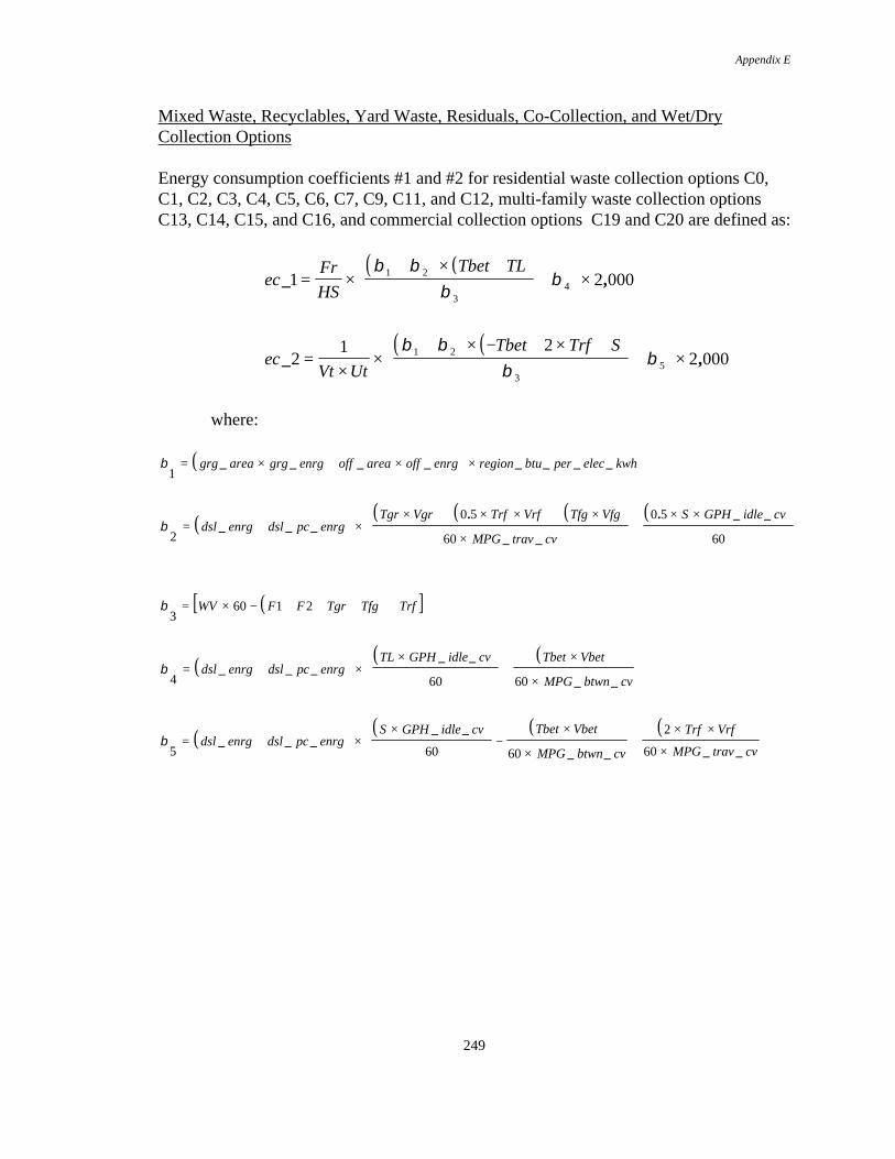
Appendix E
249
Mixed Waste, Recyclables, Yard Waste, Residuals, Co-Collection, and Wet/DryCollection Options
Energy consumption coefficients #1 and #2 for residential waste collection options C0,C1, C2, C3, C4, C5, C6, C7, C9, C11, and C12, multi-family waste collection optionsC13, C14, C15, and C16, and commercial collection options C19 and C20 are defined as:
( ) ( )ec
FrHS
Tbet TL_ ,1 2 0001 2
34= ×
+ × ++
×
β ββ
β
( ) ( )ec
Vt Ut
Tbet Trf S_ ,2
1 22 0001 2
35=
××
+ × − + × ++
×
β ββ
β
where:
( )β1
= × + × ×grg area grg enrg off area off enrg region btu per elec kwh_ _ _ _ _ _ _ _
( ) ( ) ( ) ( ) ( )β
2
0 5
60
0 5
60= + ×
× + × × + ×
×+
× ×
dsl enrg dsl pc enrg
Tgr Vgr Trf Vrf Tfg Vfg
MPG trav cv
S GPH idle cv_ _ _
.
_ _
. _ _
( )[ ]β3
60 1 2= × − + + + +WV F F Tgr Tfg Trf
( ) ( ) ( )β
4 60 60= + ×
×+
×
×
dsl enrg dsl pc enrg
TL GPH idle cv Tbet Vbet
MPG btwn cv_ _ _
_ _
_ _
( ) ( ) ( ) ( )β
5 60 60
2
60= + ×
×−
×
×+
× ×
×
dsl enrg dsl pc enrg
S GPH idle cv Tbet Vbet
MPG btwn cv
Trf Vrf
MPG trav cv_ _ _
_ _
_ _ _ _
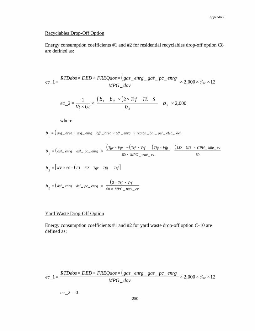
Appendix E
250
Recyclables Drop-Off Option
Energy consumption coefficients #1 and #2 for residential recyclables drop-off option C8are defined as:
( )ec
RTDdos DED FREQdos gas enrg gas pc enrg
MPG dov_
_ _ _ _
_,1 2 000 127
365=× × ×
× × ×
( ) ( )ec
Vt Ut
Trf TL S_ ,2
1 22 0001 2
35=
××
+ × × + ++
×
β ββ
β
where:
( )β1
= × + × ×grg area grg enrg off area off enrg region btu per elec kwh_ _ _ _ _ _ _ _
( ) ( ) ( ) ( ) ( )β
2 60 60= + ×
× − × + ×
×+
+ ×
dsl enrg dsl pc enrg
Tgr Vgr Trf Vrf Tfg Vfg
MPG trav cv
LD UD GPH idle cv_ _ _
_ _
_ _
( )[ ]β3
60 1 2= × − + + + +WV F F Tgr Tfg Trf
( ) ( )β
5
2
60= + ×
× ×
×
dsl enrg dsl pc enrg
Trf Vrf
MPG trav cv_ _ _
_ _
Yard Waste Drop-Off Option
Energy consumption coefficients #1 and #2 for yard waste drop-off option C-10 aredefined as:
( )ec
RTDdos DED FREQdos gas enrg gas pc enrg
MPG dov_
_ _ _ _
_,1 2 000 127
365=× × ×
× × ×
ec _2 0=
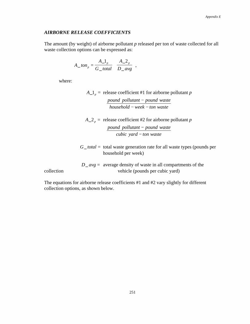
Appendix E
251
AIRBORNE RELEASE COEFFICIENTS
The amount (by weight) of airborne pollutant p released per ton of waste collected for allwaste collection options can be expressed as:
A tonA
G total
A
D avgp
p p_
_
_
_
_= +
1 2 ,
where:
A p_1 = release coefficient #1 for airborne pollutant p
pound pollutant pound waste−− −
household week ton waste
A p_2 = release coefficient #2 for airborne pollutant p
pound pollutant pound waste−−
cubic yard ton waste
G total_ = total waste generation rate for all waste types (pounds per household per week)
D avg_ = average density of waste in all compartments of thecollection vehicle (pounds per cubic yard)
The equations for airborne release coefficients #1 and #2 vary slightly for differentcollection options, as shown below.
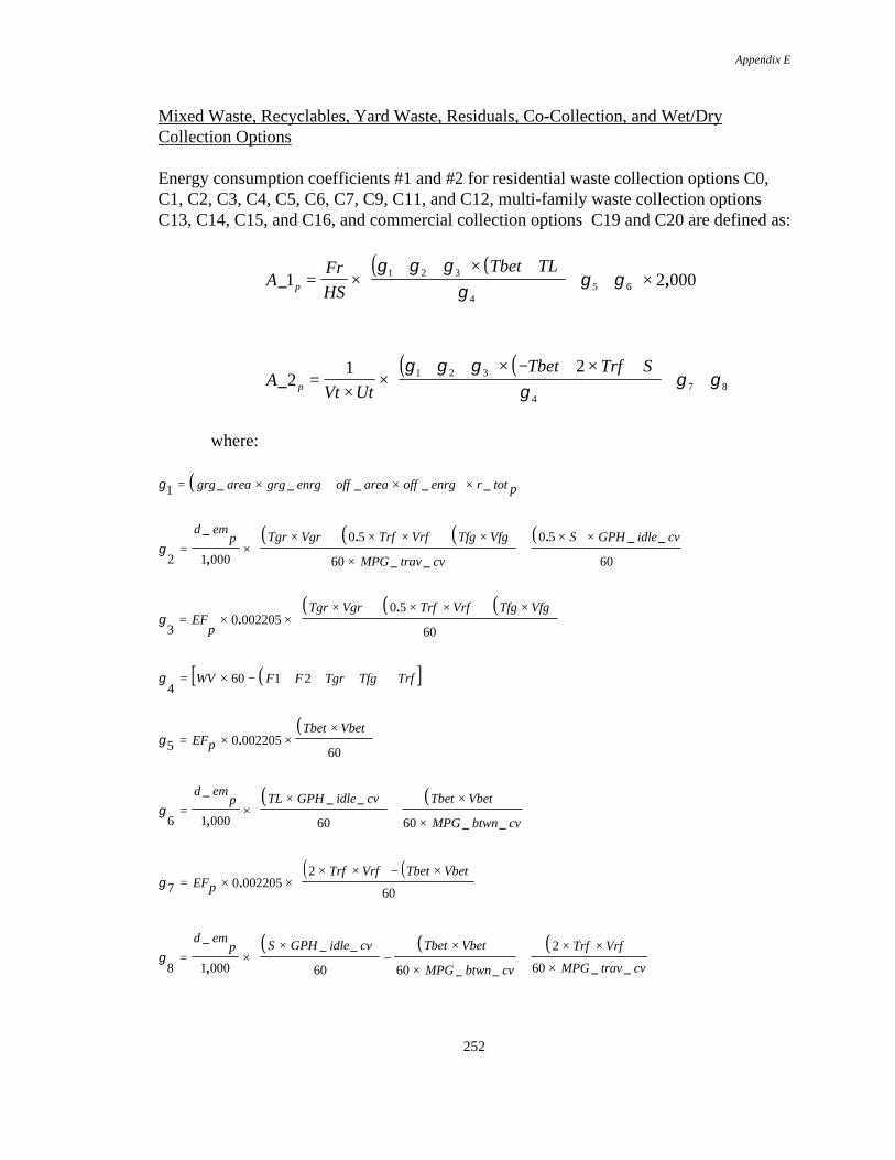
Appendix E
252
Mixed Waste, Recyclables, Yard Waste, Residuals, Co-Collection, and Wet/DryCollection Options
Energy consumption coefficients #1 and #2 for residential waste collection options C0,C1, C2, C3, C4, C5, C6, C7, C9, C11, and C12, multi-family waste collection optionsC13, C14, C15, and C16, and commercial collection options C19 and C20 are defined as:
( ) ( )A
FrHS
Tbet TLp_ ,1 2 0001 2 3
45 6= ×
+ + × ++ +
×
γ γ γγ
γ γ
( ) ( )A
Vt Ut
Tbet Trf Sp_2
1 21 2 3
47 8=
××
+ + × − + × ++ +
γ γ γγ
γ γ
where:
( )γ 1 = × + × ×grg area grg enrg off area off enrg r tot p_ _ _ _ _
( ) ( ) ( ) ( )γ
2 1 000
0 5
60
0 5
60= ×
× + × × + ×
×+
× ×
d em
p Tgr Vgr Trf Vrf Tfg Vfg
MPG trav cv
S GPH idle cv_
,
.
_ _
. _ _
( ) ( ) ( )γ
30 002205
0 5
60= × ×
× + × × + ×
EF
p
Tgr Vgr Trf Vrf Tfg Vfg.
.
( )[ ]γ4
60 1 2= × − + + + +WV F F Tgr Tfg Trf
( )γ 5 0 002205
60= × ×
×EFp
Tbet Vbet.
( ) ( )γ
6 1 000 60 60= ×
×+
×
×
d emp TL GPH idle cv Tbet Vbet
MPG btwn cv
_
,
_ _
_ _
( ) ( )γ 7 0 002205
2
60= × ×
× × − ×
EFp
Trf Vrf Tbet Vbet.
( ) ( ) ( )γ
8 1 000 60 60
2
60= ×
×−
×
×+
× ×
×
d emp S GPH idle cv Tbet Vbet
MPG btwn cv
Trf Vrf
MPG trav cv
_
,
_ _
_ _ _ _
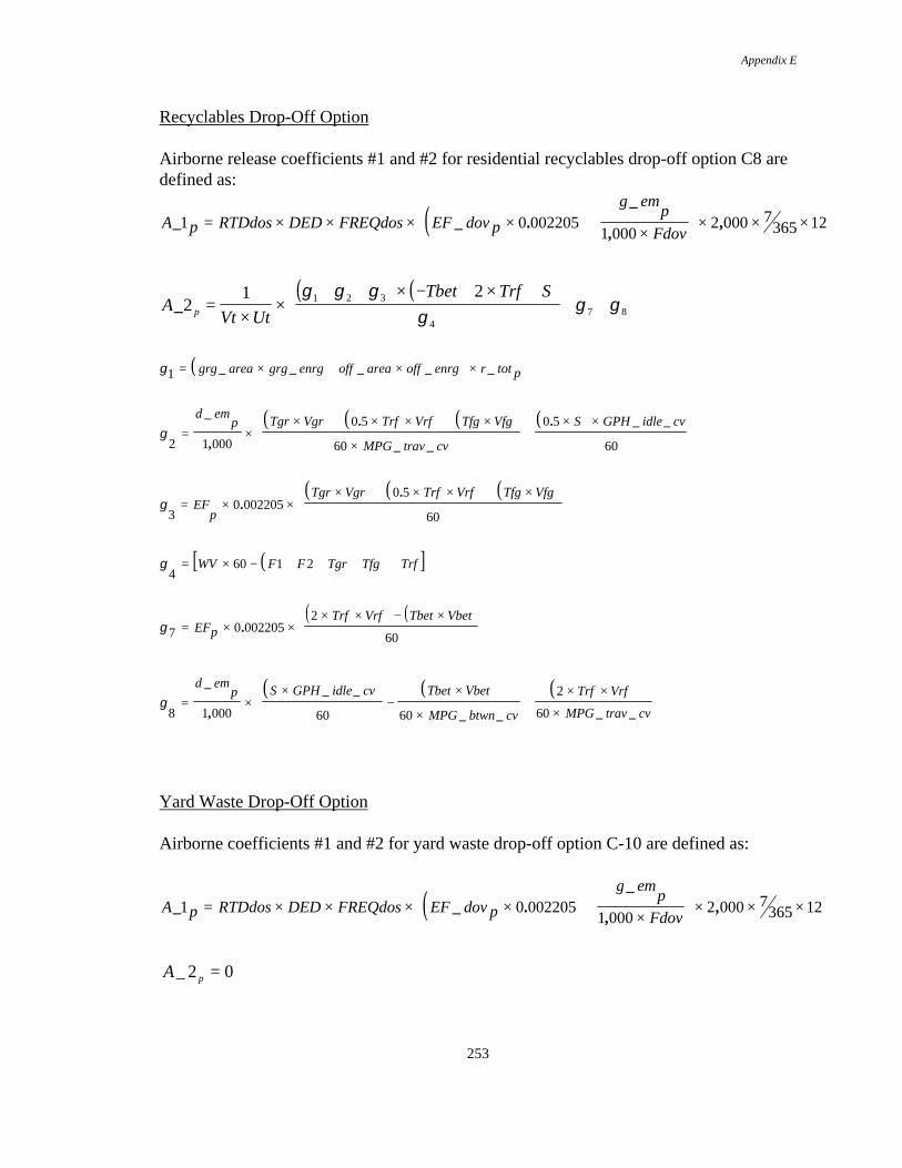
Appendix E
253
Recyclables Drop-Off Option
Airborne release coefficients #1 and #2 for residential recyclables drop-off option C8 aredefined as:
( )A p RTDdos DED FREQdos EF dov p
g emp
Fdov_ _ .
_
,,1 0 002205
1 0002 000 7
365 12= × × × × +×
× × ×
( ) ( )A
Vt Ut
Tbet Trf Sp_2
1 21 2 3
47 8=
××
+ + × − + × ++ +
γ γ γγ
γ γ
( )γ 1 = × + × ×grg area grg enrg off area off enrg r tot p_ _ _ _ _
( ) ( ) ( ) ( )γ
2 1 000
0 5
60
0 5
60= ×
× + × × + ×
×+
× ×
d em
p Tgr Vgr Trf Vrf Tfg Vfg
MPG trav cv
S GPH idle cv_
,
.
_ _
. _ _
( ) ( ) ( )γ
30 002205
0 5
60= × ×
× + × × + ×
EF
p
Tgr Vgr Trf Vrf Tfg Vfg.
.
( )[ ]γ4
60 1 2= × − + + + +WV F F Tgr Tfg Trf
( ) ( )γ 7 0 002205
2
60= × ×
× × − ×
EFp
Trf Vrf Tbet Vbet.
( ) ( ) ( )γ
8 1 000 60 60
2
60= ×
×−
×
×+
× ×
×
d emp S GPH idle cv Tbet Vbet
MPG btwn cv
Trf Vrf
MPG trav cv
_
,
_ _
_ _ _ _
Yard Waste Drop-Off Option
Airborne coefficients #1 and #2 for yard waste drop-off option C-10 are defined as:
( )A p RTDdos DED FREQdos EF dov p
g emp
Fdov_ _ .
_
,,1 0 002205
1 0002 000 7
365 12= × × × × +×
× × ×
02_ =pA

Appendix E
254
WATERBORNE RELEASE COEFFICIENTS
Similar to airborne releases, the amount (by weight) of waterborne pollutant p releasedper ton of waste collected for all waste collection options can be expressed as:
ppp
p WavgD
W
totalG
WtonW 3_
_
2_
_
1__ ++= ,
where:
=pW 1_ release coefficient #1 for waterborne pollutant p
pound pollutant pound waste−− −
household week ton waste
=pW 2_ release coefficient #2 for waterborne pollutant p
pound pollutant pound waste−−
cubic yard ton waste
=pW 3_ release coefficient #3 for waterborne pollutant p
wasteton
pollutantpound
The equations for waterborne release coefficients #1 and #2 vary slightly for differentcollection options, as shown for airborne pollutants above. For release coefficient #3, foreach collection option, this coefficient is simply:
pp RRWaterTonW ×=3_
where:
=WaterTon Gallons of wash water (garage and vehicle) used per ton ofmaterial collected (See Section 6).
=pRR User entered release rate of pollutant p in wash water
(lb./gal.)

Appendix F
255
APPENDIX F
VARIABLE NAMES

Appendix F
256
The following tables list all of the variable names used in the Collection Preprocessor.The list is divided into three sections. The first section includes names of variables in theInput Parameters section of the Collection Preprocessor spreadsheet. The second sectionlists the names of all variables for which values are calculated by the preprocessor. Thethird section lists the names of variables from other preprocessor spreadsheets that arelinked to cell formulas in the Collection Preprocessor. Each list is arrangedalphabetically.

Appendix F
257
INPUT DATA PARAMETERS - Collection Preprocessor
a = fringe benefit rate (fringe benefit $ per $ of wages)As = waterborne arsenic release rate (pounds per gallon)BOD = biochemical oxygen demand of washdown water (pounds per gallon)bv = backup rate for collection vehicles (number of backup vehicles per collectionvehicle)bw = backup rate for workers (backup workers per collection worker)c = collection vehicle operation and maintenance costs ($ per collection vehicle)Cad = waterborne cadmium release rate (pounds per gallon)CD = number of workdays per week (days per week)CFi = compaction factor for waste component i (pound per cubic yard compacted density
per pound per cubic yard as-collected density)CH4_mile_cv = airborne methane release rate from collection vehicles (grams per mile)CH4_mile_dov = airborne methane release rate from residential recyclables/yard waste
drop-off vehicles (grams per mile)CO_mile_cv = airborne carbon monoxide release rate from collection vehicles (grams per
mile)CO_mile_dov = airborne carbon monoxide release rate from residential recyclables/yard
waste drop-off vehicle (grams per mile)CO2bm_mile_cv = airborne biomass carbon dioxide release rate from collection vehicles
(grams per mile)CO2bm_mile_dov = airborne biomass carbon dioxide release rate from residential
recyclables/yard waste drop-off vehicles (grams per mile)CO2f_mile_cv = airborne fossil carbon dioxide release rate from collection vehicles(grams per mile)CO2f_mile_dov = airborne fossil carbon dioxide release rate from residential
recyclables/yard waste drop-off vehicles (grams per mile)COD = chemical oxygen demand washdown water (pounds per gallon)cri = recyclable material capture rate for component i of a mixed waste streamCr = waterborne chromium release rate (pounds per gallon)Cu = waterborne copper release rate (pounds per gallon)d = other expenses associated with collection operations ($ per collection worker per
year)d_dry = user-specified collection vehicle dry waste compartment compaction density
(pounds per cubic yard)d_msw = user-specified collection vehicle mixed waste compartment compaction density
(pounds per cubic yard)d_recyc = user-specified collection vehicle recyclables compartment compaction density
(pounds per cubic yard)d_residual = user-specified collection vehicle residual waste compartment compaction
density (pounds per cubic yard)d_wet = user-specified collection vehicle wet waste compartment compaction density
(pounds per cubic yard)
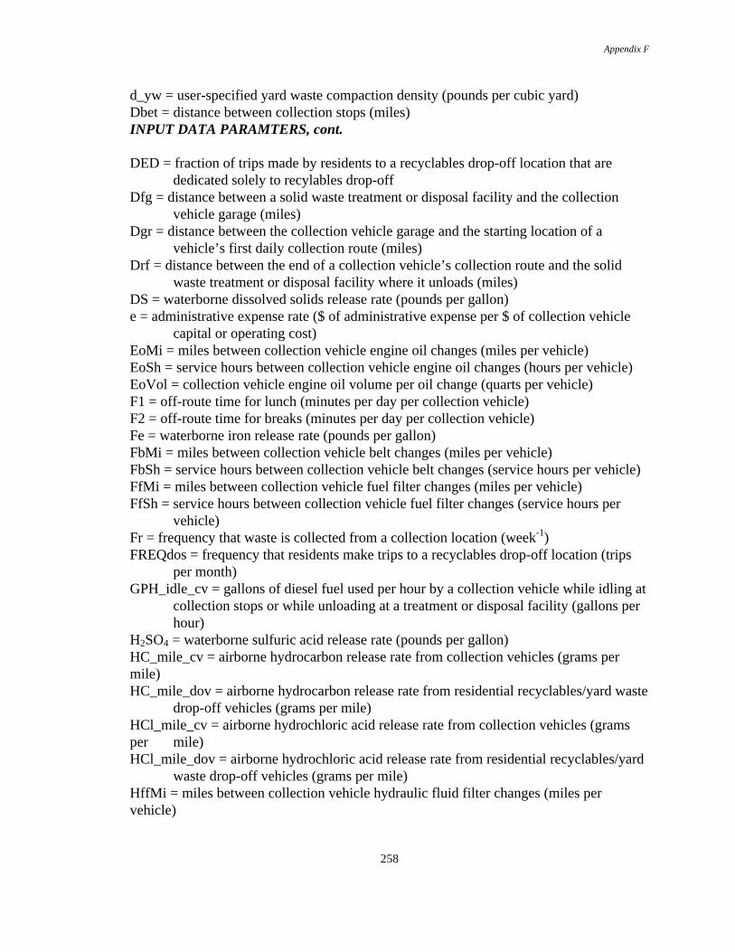
Appendix F
258
d_yw = user-specified yard waste compaction density (pounds per cubic yard)Dbet = distance between collection stops (miles)INPUT DATA PARAMTERS, cont.
DED = fraction of trips made by residents to a recyclables drop-off location that are dedicated solely to recylables drop-off
Dfg = distance between a solid waste treatment or disposal facility and the collection vehicle garage (miles)
Dgr = distance between the collection vehicle garage and the starting location of a vehicle’s first daily collection route (miles)
Drf = distance between the end of a collection vehicle’s collection route and the solid waste treatment or disposal facility where it unloads (miles)
DS = waterborne dissolved solids release rate (pounds per gallon)e = administrative expense rate ($ of administrative expense per $ of collection vehicle
capital or operating cost)EoMi = miles between collection vehicle engine oil changes (miles per vehicle)EoSh = service hours between collection vehicle engine oil changes (hours per vehicle)EoVol = collection vehicle engine oil volume per oil change (quarts per vehicle)F1 = off-route time for lunch (minutes per day per collection vehicle)F2 = off-route time for breaks (minutes per day per collection vehicle)Fe = waterborne iron release rate (pounds per gallon)FbMi = miles between collection vehicle belt changes (miles per vehicle)FbSh = service hours between collection vehicle belt changes (service hours per vehicle)FfMi = miles between collection vehicle fuel filter changes (miles per vehicle)FfSh = service hours between collection vehicle fuel filter changes (service hours per
vehicle)Fr = frequency that waste is collected from a collection location (week-1)FREQdos = frequency that residents make trips to a recyclables drop-off location (trips
per month)GPH_idle_cv = gallons of diesel fuel used per hour by a collection vehicle while idling at
collection stops or while unloading at a treatment or disposal facility (gallons per hour)
H2SO4 = waterborne sulfuric acid release rate (pounds per gallon)HC_mile_cv = airborne hydrocarbon release rate from collection vehicles (grams permile)HC_mile_dov = airborne hydrocarbon release rate from residential recyclables/yard waste
drop-off vehicles (grams per mile)HCl_mile_cv = airborne hydrochloric acid release rate from collection vehicles (gramsper mile)HCl_mile_dov = airborne hydrochloric acid release rate from residential recyclables/yard
waste drop-off vehicles (grams per mile)HffMi = miles between collection vehicle hydraulic fluid filter changes (miles pervehicle)

Appendix F
259
HffSh = service hours between collection vehicle hydraulic fluid filter changes (miles per vehicle)
HfMi = miles between collection vehicle hydraulic fluid changes (miles per vehicle)HfSh = service hours between collection vehicle hydraulic fluid changes (miles pervehicle)HfVol = collection vehicle hydraulic fluid volume per change (quarts per vehicle)Hg = waterborne mercury release rate (pounds per gallon)INPUT DATA PARMETERS, cont.
HS = number of households whose waste is collected at one collection location (households per location)
Lb = economic life of a recyclables bin (years)Lt = economic life of a collection vehicle (years)maint_area = collection vehicle garage maintenance area per vehicle (square feet per
vehicle)maint_elec = collection vehicle garage maintenance area electricity consumption rate
(kilowatts per day per square foot)maint_wd_vol = water volume required to wash down the collection vehicle garage
maintenance area (gallons per day per square foot)MPG_btwn_cv = collection vehicle diesel fuel usage rate while traveling between
collection locations (miles per gallon)MPG_dov = gasoline usage rate of vehicles driven by residents while transporting
recylables to a drop-off location (miles per gallon)MPG_trav_cv = collection vehicle diesel fuel usage rate while traveling between the
garage and the start of the first collection route; the end of a collection route and the treatment or disposal facility; or the treatment or disposal facility and the garage (miles per gallon)
NOx_mile_cv = airborne nitrogen oxides release rate from collection vehicles (grams per mile)
NOx_mile_dov = airborne nitrogen oxides release rate from residential recyclables/yard waste drop-off vehicles (grams per mile)
NH3_mile_cv = airborne ammonia release rate from collection vehicles (grams per mile)NH3_mile_dov = airborne ammonia release rate from residential recyclables/yard waste
drop-off vehicles (grams per mile)Nw = number of collection workers (excluding the driver) on one collection vehicle
(workers per vehicle)off_area = collection vehicle garage office area per collection vehicle (square feet per
vehicle)off_elec = collection vehicle office area electricity consumption rate (kilowatt hours per
day per square foot)OfMi = miles between collection vehicle engine oil filter changes (miles per vehicle)OfSh = service hours between collection vehicle engine oil filter changes (service hours
per vehicle)Oil = waterborne oil release rate (pounds per gallon)

Appendix F
260
option_frac = fraction of residential households, multi-family dwelling residents, or commercial businesses served by a collection option
P_x = waterborne phosphate release rate (pounds per gallon)Pb = unit price of a recyclables bin ($ per bin)Pb_mile_cv = airborne lead release rate from collection vehicles (grams per mile)Pb_mile_dov = airborne lead release rate from residential recyclables/yard waste drop-off
vehicles (grams per mile)
INPUT DATA PARAMETERS, cont.
PF = participation factor (fraction of residential households, multi-family dwelling residents, or commercial businesses participating in a recyclable material or yard waste collection or drop-off program)
PM_mile_cv = airborne total particulates release rate from collection vehicles (grams per mile)
PM_mile_dov = airborne total particulates release rate from residential recyclables/yard waste drop-off vehicles (grams per mile)
PM10_mile_cv = airborne release rate of particulates smaller than 10 microns from collection vehicles (grams per mile)
PM10_mile_dov = airborne release rate of particulates smaller than 10 microns from residential recyclables/yard waste drop-off vehicles (grams per mile)
Pt = unit price of a collection vehicle ($ per vehicle)Rb = number of recylables bins per household (bins per household)RTDdos = round trip distance driven by resident while transporting recylables to a drop-
off location (miles per trip)S = time to unload a collection vehicle at a treatment or disposal facility (minutes per trip)Se = waterborne selenium release rate (pounds per gallon)SS = waterborne suspended solids release rate (pounds per gallon)SOx_mile_cv = airborne sulfur oxides release rate from collection vehicles (grams per
mile)SOx_mile_dov = airborne sulfur oxides release rate from residential recyclables/yardwaste drop-off vehicles (grams per mile)Tbtw = collection vehicle travel time between collection locations (minutes per location)Tfg = collection vehicle travel time between the treatment or disposal facility and the
garage (minutes per day per vehicle)TfMi = miles between collection vehicle transmission fluid changes (miles per vehicle)TfSh = service hours between collection vehicle transmission fluid changes (servicehours per vehicle)Tgr = collection vehicle travel time between garage and start of first collection route
(minutes per day per vehicle)TireMi = miles between collection vehicle tire change (miles per vehicle)TireNum = number of tires on a collection vehicle (tires per vehicle)TireSh = service hours between collection vehicle tire change (service hours per vehicle)TL = collection vehicle loading time at collection location (minutes per location)
Appendix F
261
Trf = collection vehicle travel time between end of collection route and solid waste treatment or disposal facility)
Ut = collection vehicle utilization factor (useable cubic yards of vehicle capacity per total cubic yards of vehicle capacity)
Vbet = collection vehicle travel speed between collection locations (miles per hour)Vfg = collection vehicle speed while traveling between the solid waste treatment or
disposal facility and the garageVgr = collection vehicle speed while traveling between the garage and the start of the first
collection route (miles per hour)INPUT DATA PARAMETERS, cont.
Vrf = collection vehicle speed while traveling between the end of a collection route and the solid waste treatment or disposal facility (miles per hour)
Vt = collection vehicle capacity (cubic yards)W_NH3 = waterborne ammonia release rate (pounds per gallon)W_Pb = waterborne lead release rate (pounds per gallon)Wa = hourly wage for a collection worker other than a vehicle driver ($ per hour)Wd = hourly wage for a collection vehicle driver ($ per hour)WdMi = miles between collection vehicle washdowns (miles per vehicle)WdSh = service hours between collection vehicle washdowns (service hours per vehicle)WdVol = water volume per collection vehicle washdown (gallons per vehicle)WP = working hours per day for which collection workers and vehicle drivers receive
wages (hours per day)WV = hours per day that collection vehicle are in use (hours per day)Zn = waterborne zinc release rate (pounds per gallon)
Appendix F
262
CALCULATED PARAMETERS - Collection Preprocessor
C_ann = annual collection cost, including capital and operating costs ($ per year)C_cap_b = annualized capital cost of recyclables bins at locations served by onecollection vehicle ($ per vehicle per year)C_cap_v = annualized capital cost of a collection vehicle ($ per vehicle per year)C_house = annual collection cost per residential household ($ per household)C_location = annual collection cost per multi-family or commercial waste collection
location ($ per location)C_op = annual collection vehicle operating costs ($ per vehicle per year)C_ton = collection cost per ton of material collected ($ per ton)C_vehicle = annual collection cost per collection vehicle ($ per vehicle)Cb = annualized capital cost of a recylables bin ($ per bin per year)Coe = annual cost of other collection vehicle operating expenses ($ per vehicle per year)Cvo = annual collection vehicle operating and maintenance costs ($ per vehicle per year)Cw = annual collection vehicle labor costs ($ per vehicle per year)D_avg = average density of all waste collected in a multi-compartment collection vehicle
(pounds per cubic yard)D_dry = in-truck density of dry waste (pounds per cubic yard)D_msw = in-truck density of mixed waste (pounds per cubic yard)D_recyc = in-truck density of recyclables (pounds per cubic yard)D_residual = in-truck density of residual waste (pounds per cubic yard)D_wet = in-truck density of wet waste (pounds per cubic yard)D_yw = in-truck density of yard waste (pounds per cubic yard)Db = cumulative distance that a collection vehicle travels between collection stops perday (miles per vehicle per day)DF_R = cumulative distance that a collection vehicle travels between the start/end points
of its collection routes and the solid waste treatment or disposal facility (miles per vehicle per day)
DF_S = cumulative distance that a collection vehicle travels between a residential recyclables drop-off site and the material recovery facility per day (miles per vehicle per day)
ElecD = daily amount of electricity consumed at the collection vehicle garage per vehicle (kilowatts per vehicle per day)
ElecTon = collection vehicle garage electricity usage per ton of material collected (kilowatts per ton)
F_R = cumulative collection vehicle travel time between the start/end points of its collection routes and the solid waste treatment or disposal facility (minutes per vehicle per day)
frac_cap_recyc = captured recyclables fraction (pounds of recyclables separated from the waste stream per total pounds of waste material)
frac_dry = fraction of waste collected in the dry compartment of a wet/dry or wet/dry/recyclables collection vehicle (pounds of dry waste per total pounds of waste material)

Appendix F
263
CALCULATED PARAMETERS, cont.
frac_wet = fraction of waste collected in the wet compartment of a wet/dry or wet/dry/recyclables collection vehicle (pounds of dry waste per total pounds of waste material)
frac_yw = fraction of yard waste (pounds of yard waste per total pounds of waste material)
FuelD = daily volume of fuel consumed by a collection vehicle (gallons per vehicle per day)
FuelT = residential recyclables/yard waste drop-off vehicle fuel usage per round trip to and from the drop-off site (gallons per trip)
FuelTon = collection vehicle fuel usage per ton of material collected (gallons per ton)FuelTon_dov = residential recyclables/yard waste drop-off vehicle fuel usage per ton of
material delivered to the drop-off site (gallons per ton)G_dry = dry waste generation rate (pounds per household or collection location per week)G_msw = mixed waste generation rate (pounds per household or collection location per
week)G_recyc = recyclables generation rate (pounds per household or collection location per
week)G_residual = residual waste generation rate (pounds per household or collection location
per week)G_total = total generation rate for all waste categories (pounds per household or
collection location per week)G_wet = wet waste generation rate (pounds per household or collection location per
week)G_yw = yard waste generation rate (pounds per household or collection location per
week)Ht = number of collection locations that a collection vehicle stops at to collect material
during one collection trip (locations per trip)LD = cumulative time that a collection vehicle spends loading material at collection stops
per day (minutes per vehicle per day)MiD = daily miles traveled by a collection vehicle (miles per vehicle per day)Nb = number of recyclables bins at locations served by one collection vehicle (bins per
vehicle)Nt = number of collection vehicles (vehicles)RD = daily number of collection trips by one collection vehicle (trips per vehicle per day)RefD = daily weight of material collected by one collection vehicle (tons per vehicle per
day)RefT = weight of residential recyclables or yard waste delivered to the drop-off site per
trip (pounds per trip)Rt = number of collection vehicle trips needed to collect all of the recyclable material that
collects at a residential recyclables drop-off location in one week (trips per week)
Appendix F
264
RT = number of collection vehicle trips needed to service all of the collection locations served by a particular collection option during one collection cycle (trips per
cycle)
CALCULATED PARAMETERS, cont.
ShD = number of service hours per day for one collecti0n vehicle (hours per vehicle per day)
SD = number of collection locations that a collection vehicle stops at to collect material per day (locations per vehicle per day)
Tb = cumulative collection vehicle travel time between collection locations per day (minutes per vehicle per day)
Tbet = collection vehicle travel time between two consecutive collection locations (minutes per location)
Tc = time required for a collection vehicle to make one complete collection trip (minutes per trip)
UD = cumulative time that a collection vehicle spends unloading material at a solid wastetreatment or disposal facility per day (minutes per vehicle per day)
vol_recyc = volume of recyclables deposited at a residential drop-off site per week (cubic yards per week)
W_cv = daily volume of water used to wash down a collection vehicle (gallons pervehicle per day)W_gar = daily volume of water used to wash down the vehicle garage (gallons per vehicle
per day)WaterTon = collection vehicle water usage per ton of material collected (gallons per ton)
Appendix F
265
VARIABLE NAMES FROM OTHER PREPROCESSORS
Common Preprocessor
CH4_GWP = relative 20-year Global Warming Potential for methaneCO2_GWP = relative 20-year Global Warming Potential for carbon dioxideCOM_WT_FRAC_1i = weight fraction of waste component i in Sector #1 commercial
wastecomm_name = community named_emp = precombustion emission rate for pollutant p associated with the production of
diesel fuel (pounds of pollutant per 1,000 gallons of diesel fuel)dsl_enrg = energy content of diesel fuel (Btu per gallon)dsl_pc_enrg = precombustion energy content of diesel fuel (Btu per gallon)g_emp = precombustion emission rate for pollutant p associated with the production of
gasoline (pounds of pollutant per 1,000 gallons of gasoline)gas_enrg = energy content of gasoline (Btu per gallon)gas_pc_enrg = precombustion energy content of gasoline (Btu per gallon)HC_GWP = relative 20-year Global Warming Potential for other hydrocarbonsi = annual interest rate or yearly discount rate (year-1)mf_pop = multi-family population (persons)MF_WT_FRAC_1i = weight fraction of waste component i in Sector #1 multi-family
wasteNO_GWP = relative 20-year Global Warming Potential for nitrous oxideres_pop = residential population (persons)RES_WT_FRAC_1i = weight fraction of waste component i in Sector #1 residential
wastesf_WD_dryi = weight fraction of waste component i separated from the waste stream and
placed in a dry waste collection container for wet/dry collection options C12 and C18
sf_WD_weti = weight fraction of waste component i separated from the waste stream and placed in a wet waste collection container for wet/dry collection options C12 and C18
sf_WDR_dryi = weight fraction of waste component i separated from the waste stream and placed in a dry waste collection container for wet/dry/recyclable collection options C11 and C17
sf_WDR_recyci = weight fraction of waste component i separated from the waste stream and placed in a recyclables waste collection container for wet/dry/recyclable collection options C11 and C17
sf_WDR_weti = weight fraction of waste component i separated from the waste stream and placed in a wet waste collection container for wet/dry/recyclable collection options C11 and C17
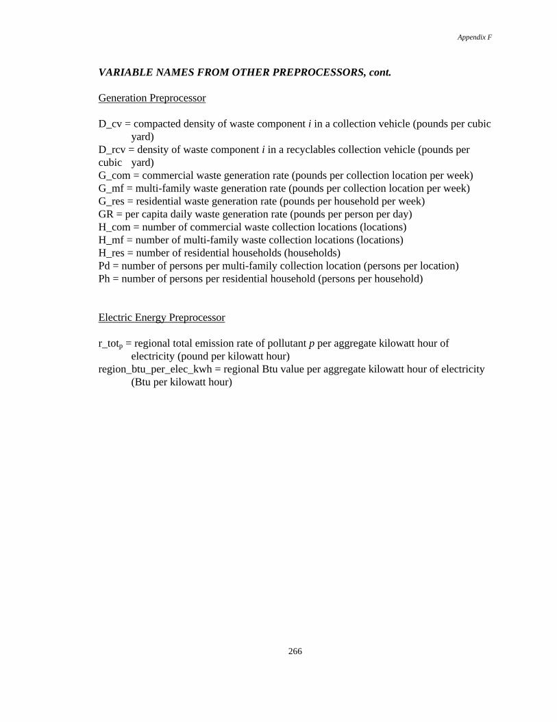
Appendix F
266
VARIABLE NAMES FROM OTHER PREPROCESSORS, cont.
Generation Preprocessor
D_cv = compacted density of waste component i in a collection vehicle (pounds per cubicyard)
D_rcv = density of waste component i in a recyclables collection vehicle (pounds percubic yard)G_com = commercial waste generation rate (pounds per collection location per week)G_mf = multi-family waste generation rate (pounds per collection location per week)G_res = residential waste generation rate (pounds per household per week)GR = per capita daily waste generation rate (pounds per person per day)H_com = number of commercial waste collection locations (locations)H_mf = number of multi-family waste collection locations (locations)H_res = number of residential households (households)Pd = number of persons per multi-family collection location (persons per location)Ph = number of persons per residential household (persons per household)
Electric Energy Preprocessor
r_totp = regional total emission rate of pollutant p per aggregate kilowatt hour of electricity (pound per kilowatt hour)
region_btu_per_elec_kwh = regional Btu value per aggregate kilowatt hour of electricity (Btu per kilowatt hour)
Appendix G
267
APPENDIX G
COST ESCALATION DATA

Appendix G
268
Appendix G - 1
DESCRIPTION VARIABLE NAME VALUECost Index for 1980 CI_1980 0.858
Cost Index for 1981 CI_1981 0.946
Cost Index for 1982 CI_1982 1.000
Cost Index for 1983 CI_1983 1.028
Cost Index for 1984 CI_1984 1.052
Cost Index for 1985 CI_1985 1.075
Cost Index for 1986 CI_1986 1.097
Cost Index for 1987 CI_1987 1.117
Cost Index for 1988 CI_1988 1.143
Cost Index for 1989 CI_1989 1.180
Cost Index for 1990 CI_1990 1.229
Cost Index for 1991 CI_1991 1.267
Cost Index for 1992 CI_1992 1.291
Cost Index for 1993 CI_1993 1.314
Cost Index for 1994 CI_1994 1.341
Cost Index for 1995 CI_1995 1.367
Cost Index for 1996 CI_1996 1.399
Cost Index for 1997 CI_1997 1.430
Cost Index for 1998 CI_1998 1.462
Cost Index for 1999 CI_1999 1.494
Cost Index for 2000 CI_2000 1.526
Cost Index for 2001 CI_2001 1.557
Cost Index for 2002 CI_2002 1.589
Cost Index for 2003 CI_2003 1.621
Cost Index for 2004 CI_2004 1.652
Cost Index for 2005 CI_2005 1.684
Model Year Override Model_yearCurrent Year Cur_year 1998
Base Year Cost Index Base_index 1.31
Current Year Cost Index CI_cur_year 1.46
Cost Index Factor CI_Factor 1.11
COST INDEX TABLE