a spectral algorithm for learning hidden markov models hdjhsu/papers/hmm-slides.pdf · a spectral...
TRANSCRIPT
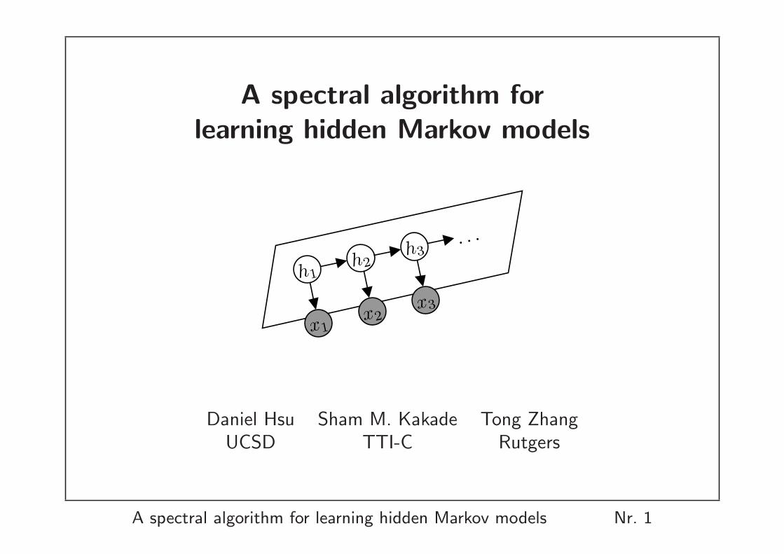
A spectral algorithm forlearning hidden Markov models
h1
x1x2
h3
x3
. . .
h2
Daniel Hsu Sham M. Kakade Tong ZhangUCSD TTI-C Rutgers
A spectral algorithm for learning hidden Markov models Nr. 1
Motivation
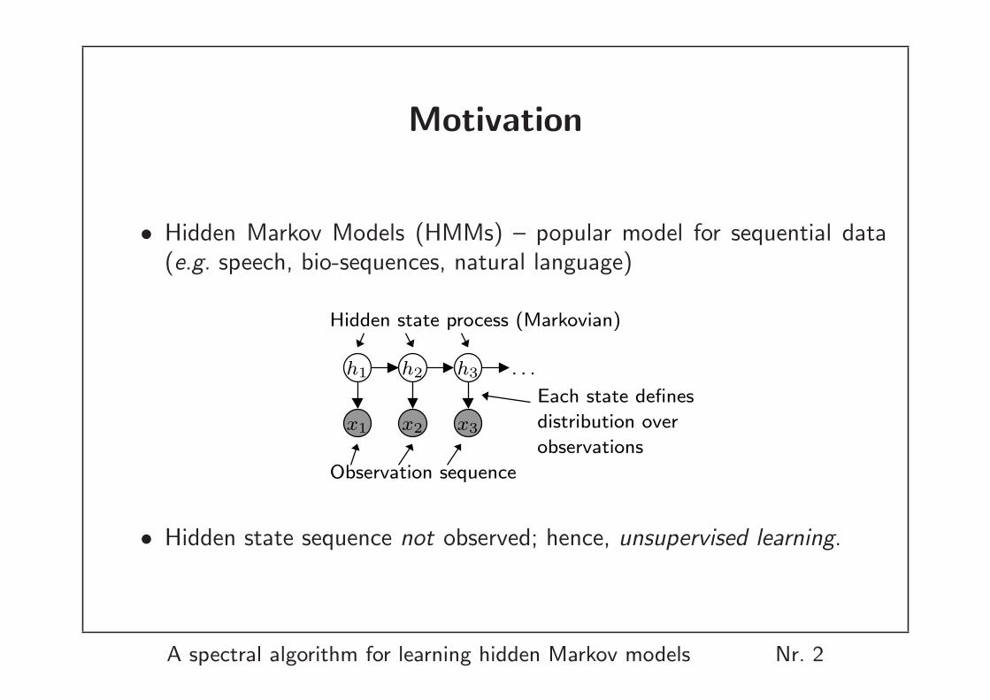
• Hidden Markov Models (HMMs) – popular model for sequential data(e.g. speech, bio-sequences, natural language)
h1
x1
h2
x2
h3
x3
. . .
Each state defines
distribution over
observations
Hidden state process (Markovian)
Observation sequence
• Hidden state sequence not observed; hence, unsupervised learning.
A spectral algorithm for learning hidden Markov models Nr. 2
Motivation
• Why HMMs?
– Handle temporally-dependent data
– Succinct “factored” representation when state space is low-dimensional(c.f. autoregressive model)
• Some uses of HMMs:
– Monitor “belief state” of dynamical system
– Infer latent variables from time series
– Density estimation
A spectral algorithm for learning hidden Markov models Nr. 3
Preliminaries: parameters of discrete HMMs
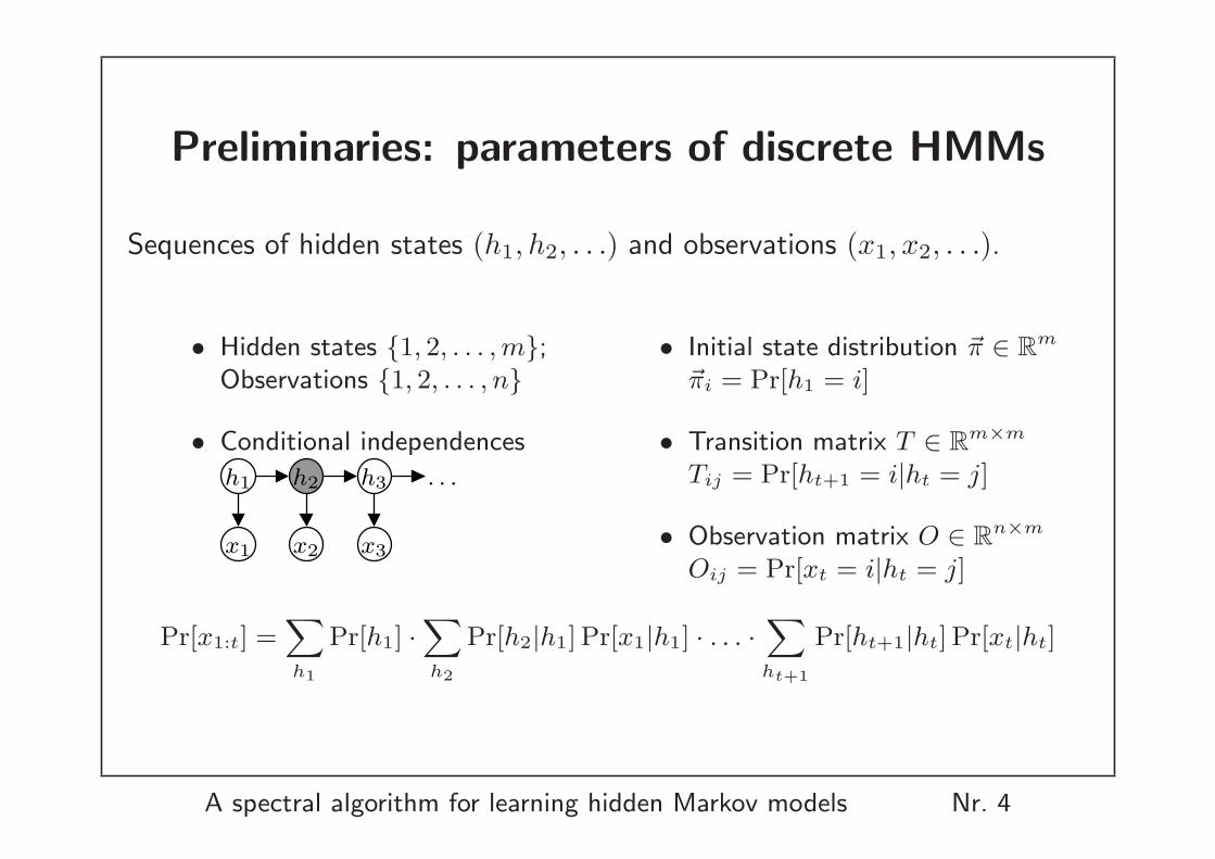
Sequences of hidden states (h1, h2, . . .) and observations (x1, x2, . . .).
• Hidden states {1, 2, . . . , m};Observations {1, 2, . . . , n}
• Conditional independences
h1
x1
h2
x2
h3
x3
. . .
• Initial state distribution ~π ∈ Rm
~πi = Pr[h1 = i]
• Transition matrix T ∈ Rm×m
Tij = Pr[ht+1 = i|ht = j]
• Observation matrix O ∈ Rn×m
Oij = Pr[xt = i|ht = j]
Pr[x1:t] =X
h1
Pr[h1] ·X
h2
Pr[h2|h1] Pr[x1|h1] · . . . ·X
ht+1
Pr[ht+1|ht] Pr[xt|ht]
A spectral algorithm for learning hidden Markov models Nr. 4
Preliminaries: learning discrete HMMs
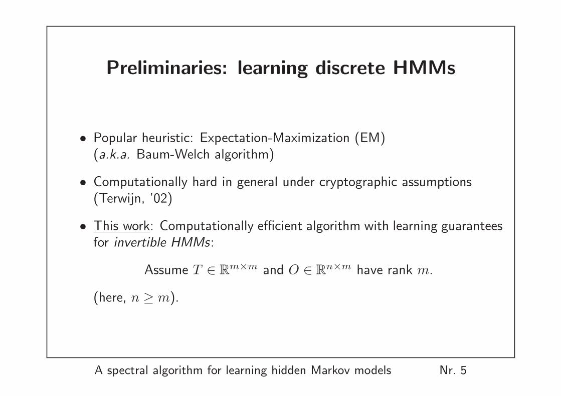
• Popular heuristic: Expectation-Maximization (EM)(a.k.a. Baum-Welch algorithm)
• Computationally hard in general under cryptographic assumptions(Terwijn, ’02)
• This work: Computationally efficient algorithm with learning guaranteesfor invertible HMMs:
Assume T ∈ Rm×m and O ∈ Rn×m have rank m.
(here, n ≥ m).
A spectral algorithm for learning hidden Markov models Nr. 5
Our contributions
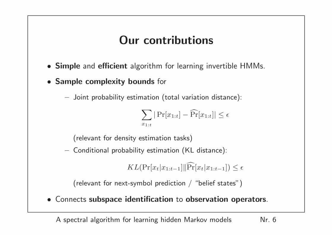
• Simple and efficient algorithm for learning invertible HMMs.
• Sample complexity bounds for
– Joint probability estimation (total variation distance):
Xx1:t
|Pr[x1:t]−cPr[x1:t]| ≤ ε
(relevant for density estimation tasks)
– Conditional probability estimation (KL distance):
KL(Pr[xt|x1:t−1]‖cPr[xt|x1:t−1]) ≤ ε
(relevant for next-symbol prediction / “belief states”)
• Connects subspace identification to observation operators.
A spectral algorithm for learning hidden Markov models Nr. 6
Outline
1. Motivation and preliminaries
2. Discrete HMMs: key ideas
3. Observable representation for HMMs
4. Learning algorithm and guarantees
5. Conclusions and future work
A spectral algorithm for learning hidden Markov models Nr. 7
Outline
1. Motivation and preliminaries
2. Discrete HMMs: key ideas
3. Observable representation for HMMs
4. Learning algorithm and guarantees
5. Conclusions and future work
A spectral algorithm for learning hidden Markov models Nr. 8
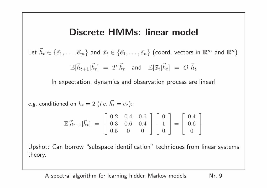
Discrete HMMs: linear model
Let ~ht ∈ {~e1, . . . , ~em} and ~xt ∈ {~e1, . . . , ~en} (coord. vectors in Rm and Rn)
E[~ht+1|~ht] = T ~ht and E[~xt|~ht] = O ~ht
In expectation, dynamics and observation process are linear!
e.g. conditioned on ht = 2 (i.e. ~ht = ~e2):
E[~ht+1|~ht] =
24
0.2 0.4 0.60.3 0.6 0.40.5 0 0
3524
010
35 =
24
0.40.60
35
Upshot: Can borrow “subspace identification” techniques from linear systemstheory.
A spectral algorithm for learning hidden Markov models Nr. 9
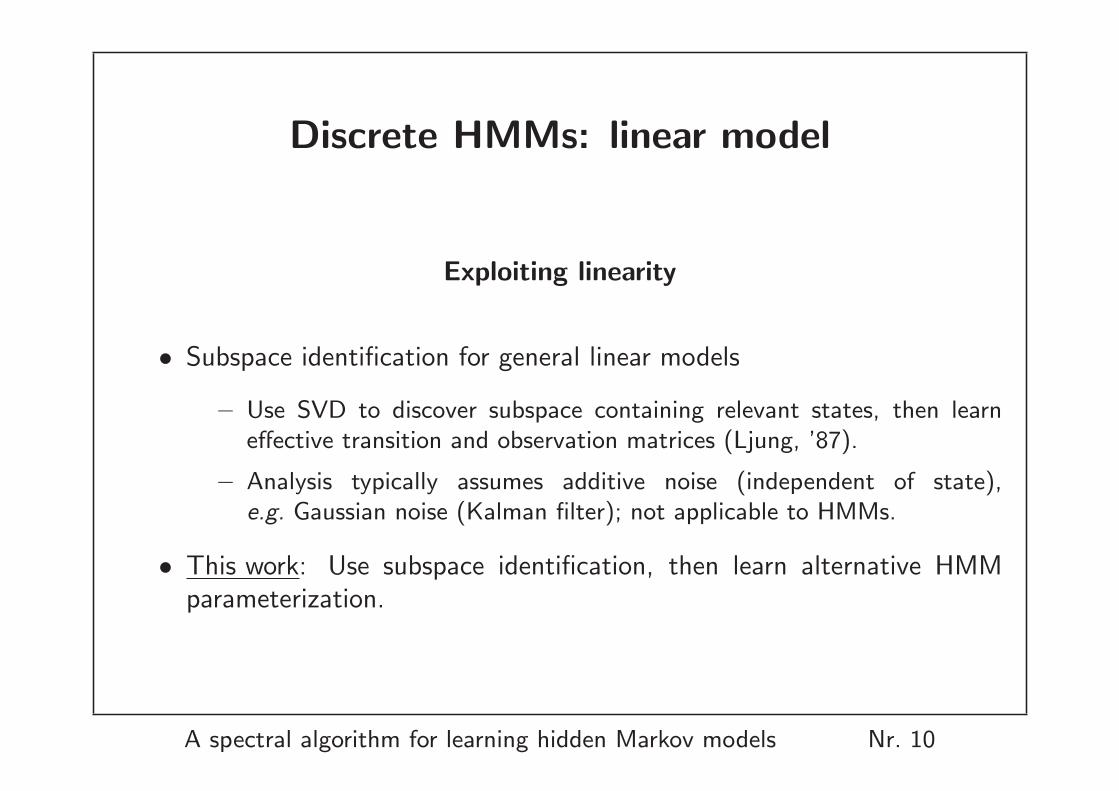
Discrete HMMs: linear model
Exploiting linearity
• Subspace identification for general linear models
– Use SVD to discover subspace containing relevant states, then learneffective transition and observation matrices (Ljung, ’87).
– Analysis typically assumes additive noise (independent of state),e.g. Gaussian noise (Kalman filter); not applicable to HMMs.
• This work: Use subspace identification, then learn alternative HMMparameterization.
A spectral algorithm for learning hidden Markov models Nr. 10

Discrete HMMs: observation operators
For x ∈ {1, . . . , n}: define
Ax4=
T
Ox,1 0. . .
0 Ox,m
∈ Rm×m
[Ax]i,j = Pr[ ht+1 = i ∧ xt = x | ht = j ].
The {Ax} are observation operators (Schutzenberger, ’61; Jaeger, ’00).
. . .T
O
xt
ht
Axt
A spectral algorithm for learning hidden Markov models Nr. 11
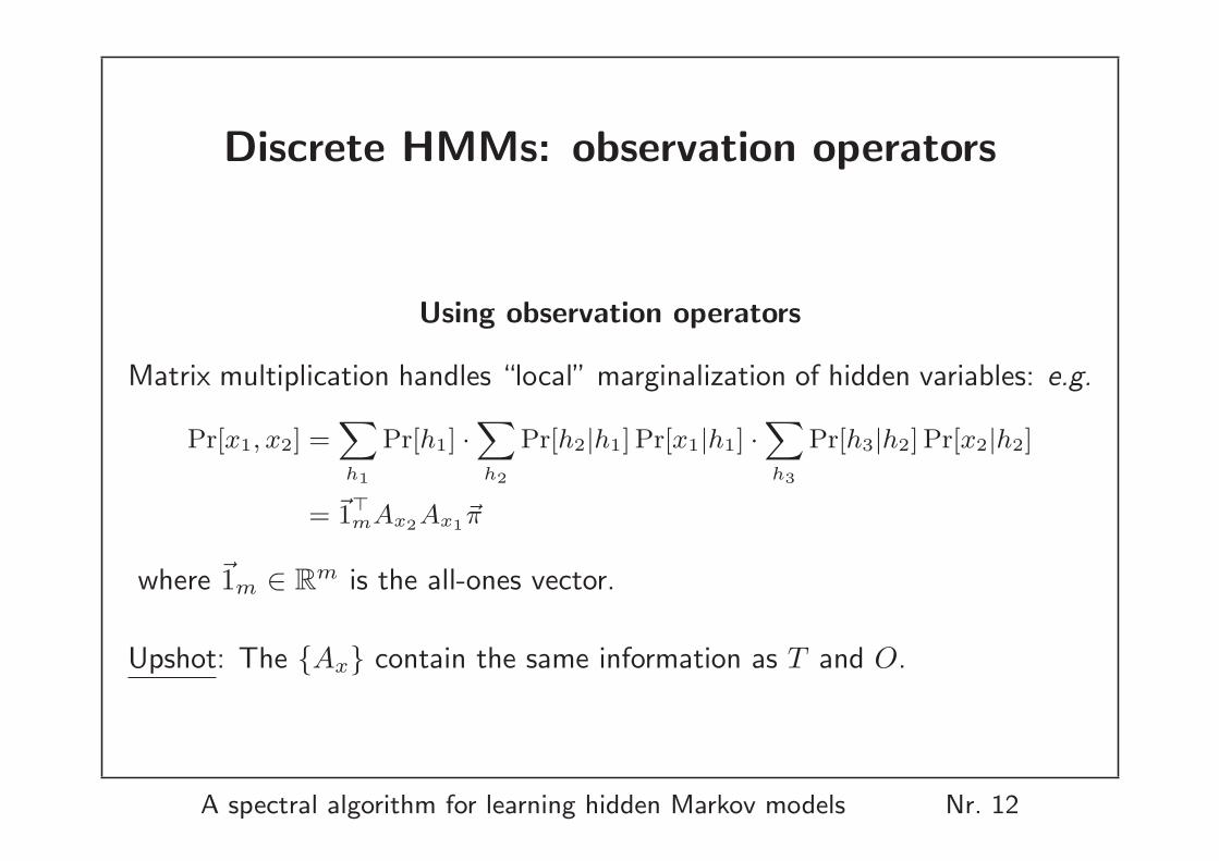
Discrete HMMs: observation operators
Using observation operators
Matrix multiplication handles “local” marginalization of hidden variables: e.g.
Pr[x1, x2] =X
h1
Pr[h1] ·X
h2
Pr[h2|h1] Pr[x1|h1] ·X
h3
Pr[h3|h2] Pr[x2|h2]
= ~1>mAx2Ax1~π
where ~1m ∈ Rm is the all-ones vector.
Upshot: The {Ax} contain the same information as T and O.
A spectral algorithm for learning hidden Markov models Nr. 12
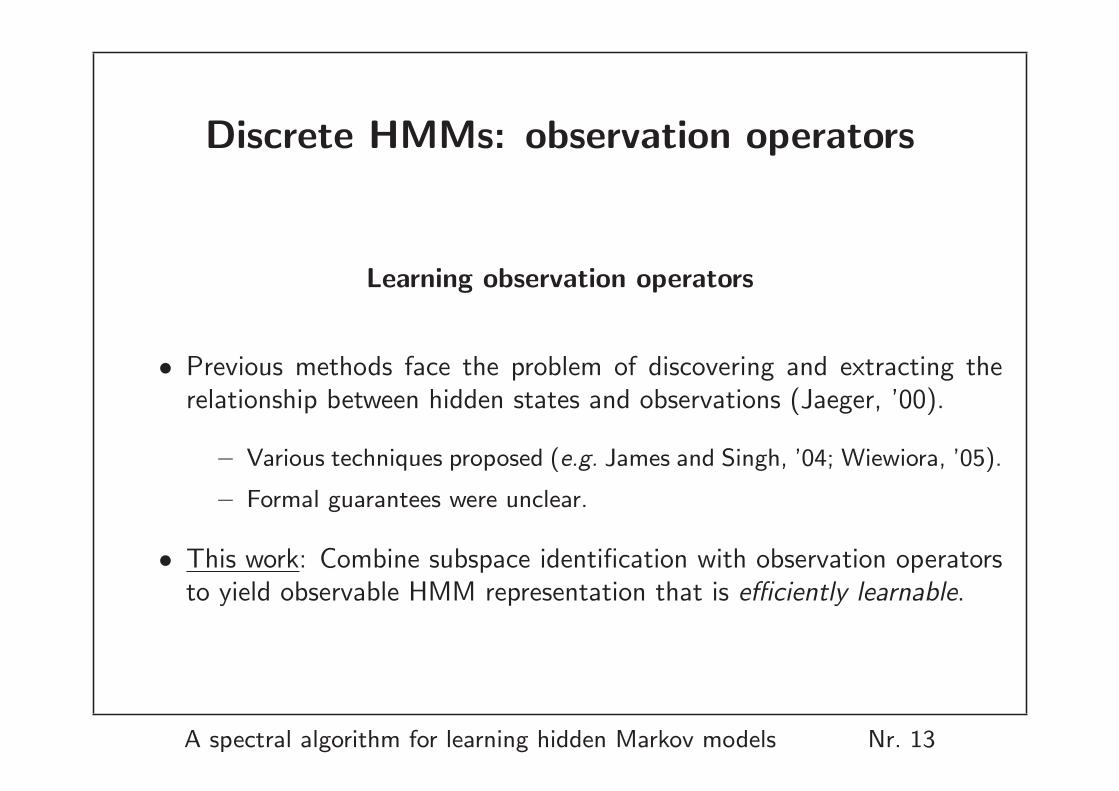
Discrete HMMs: observation operators
Learning observation operators
• Previous methods face the problem of discovering and extracting therelationship between hidden states and observations (Jaeger, ’00).
– Various techniques proposed (e.g. James and Singh, ’04; Wiewiora, ’05).
– Formal guarantees were unclear.
• This work: Combine subspace identification with observation operatorsto yield observable HMM representation that is efficiently learnable.
A spectral algorithm for learning hidden Markov models Nr. 13
Outline
1. Motivation and preliminaries
2. Discrete HMMs: key ideas
3. Observable representation for HMMs
4. Learning algorithm and guarantees
5. Conclusions and future work
A spectral algorithm for learning hidden Markov models Nr. 14
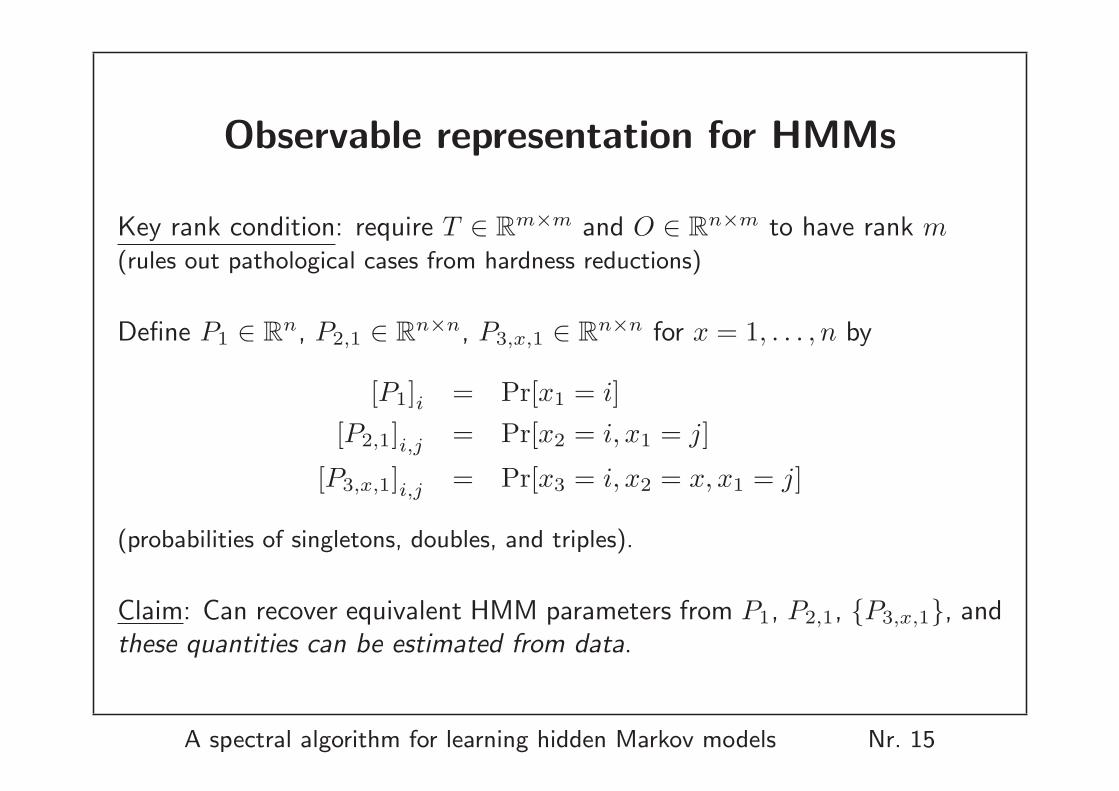
Observable representation for HMMs
Key rank condition: require T ∈ Rm×m and O ∈ Rn×m to have rank m(rules out pathological cases from hardness reductions)
Define P1 ∈ Rn, P2,1 ∈ Rn×n, P3,x,1 ∈ Rn×n for x = 1, . . . , n by
[P1]i = Pr[x1 = i][P2,1]i,j = Pr[x2 = i, x1 = j]
[P3,x,1]i,j = Pr[x3 = i, x2 = x, x1 = j]
(probabilities of singletons, doubles, and triples).
Claim: Can recover equivalent HMM parameters from P1, P2,1, {P3,x,1}, andthese quantities can be estimated from data.
A spectral algorithm for learning hidden Markov models Nr. 15
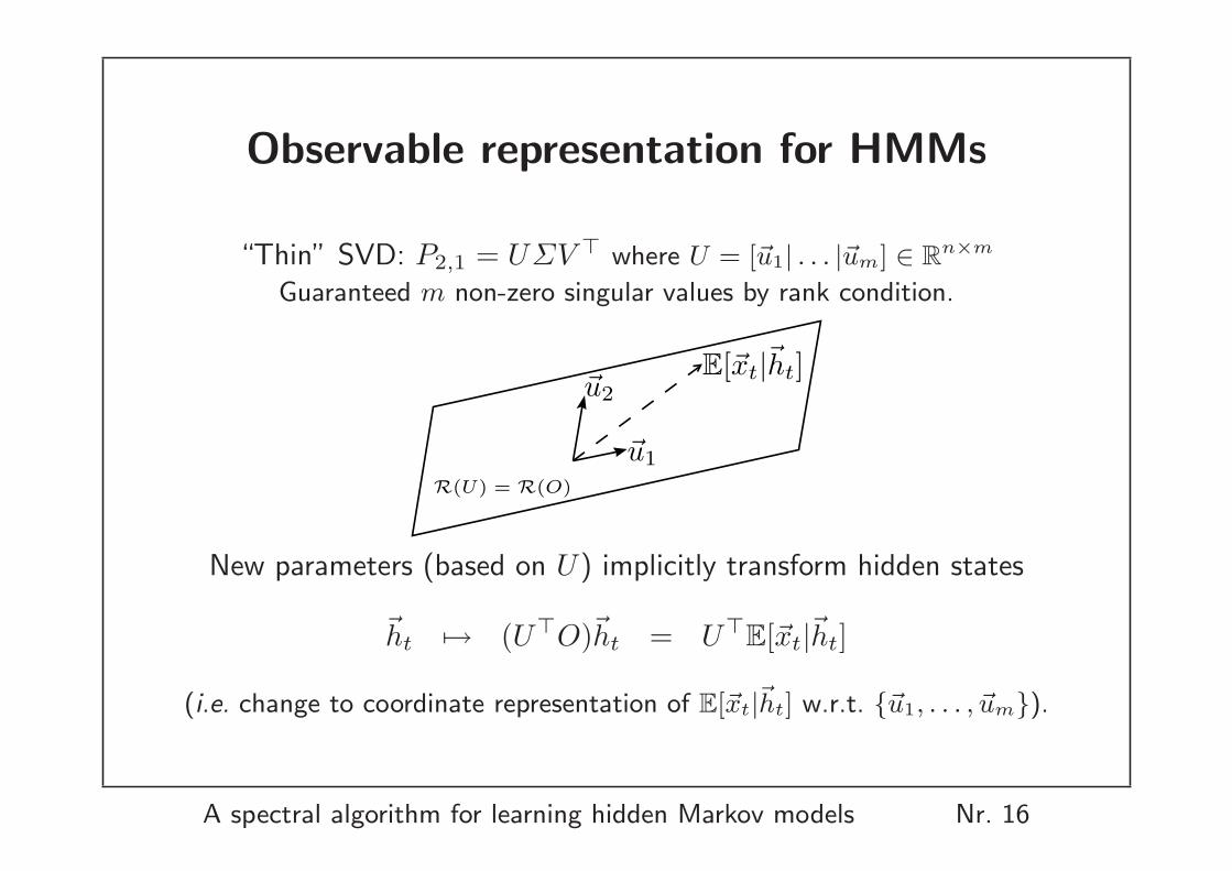
Observable representation for HMMs
“Thin” SVD: P2,1 = UΣV > where U = [~u1| . . . |~um] ∈ Rn×m
Guaranteed m non-zero singular values by rank condition.
E[~xt|~ht]~u2
~u1
R(U) = R(O)
New parameters (based on U) implicitly transform hidden states
~ht 7→ (U>O)~ht = U>E[~xt|~ht]
(i.e. change to coordinate representation of E[~xt|~ht] w.r.t. {~u1, . . . , ~um}).
A spectral algorithm for learning hidden Markov models Nr. 16
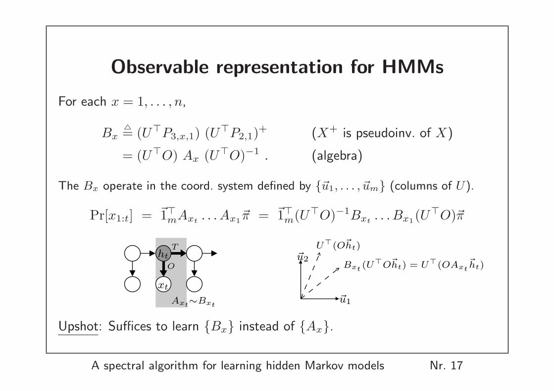
Observable representation for HMMs
For each x = 1, . . . , n,
Bx4= (U>P3,x,1) (U>P2,1)+ (X+ is pseudoinv. of X)
= (U>O) Ax (U>O)−1 . (algebra)
The Bx operate in the coord. system defined by {~u1, . . . , ~um} (columns of U).
Pr[x1:t] = ~1>mAxt . . . Ax1~π = ~1>m(U>O)−1Bxt . . . Bx1(U>O)~π
xt
O
T
Axt∼Bxt
ht
~u1
~u2
U>(O~ht)
Bxt (U>O~ht) = U>(OAxt~ht)
Upshot: Suffices to learn {Bx} instead of {Ax}.
A spectral algorithm for learning hidden Markov models Nr. 17
Outline
1. Motivation and preliminaries
2. Discrete HMMs: key ideas
3. Observable representation for HMMs
4. Learning algorithm and guarantees
5. Conclusions and future work
A spectral algorithm for learning hidden Markov models Nr. 18
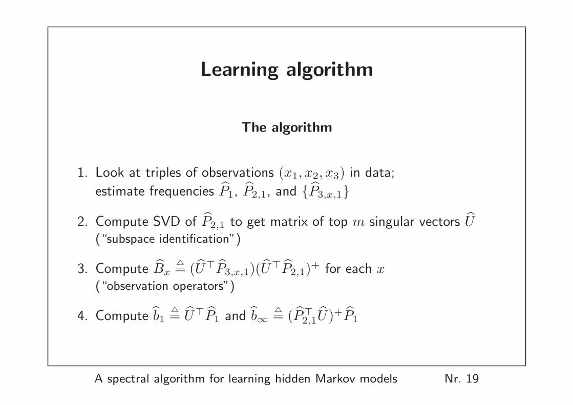
Learning algorithm
The algorithm
1. Look at triples of observations (x1, x2, x3) in data;
estimate frequencies P1, P2,1, and {P3,x,1}
2. Compute SVD of P2,1 to get matrix of top m singular vectors U(“subspace identification”)
3. Compute Bx4= (U>P3,x,1)(U>P2,1)+ for each x
(“observation operators”)
4. Compute b14= U>P1 and b∞
4= (P>2,1U)+P1
A spectral algorithm for learning hidden Markov models Nr. 19
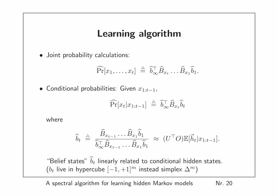
Learning algorithm
• Joint probability calculations:
Pr[x1, . . . , xt]4= b>∞Bxt . . . Bx1 b1.
• Conditional probabilities: Given x1:t−1,
Pr[xt|x1:t−1]4= b>∞Bxt bt
where
bt4=
Bxt−1 . . . Bx1 b1
b>∞Bxt−1 . . . Bx1 b1
≈ (U>O)E[~ht|x1:t−1].
“Belief states” bt linearly related to conditional hidden states.(bt live in hypercube [−1,+1]m instead simplex ∆m)
A spectral algorithm for learning hidden Markov models Nr. 20
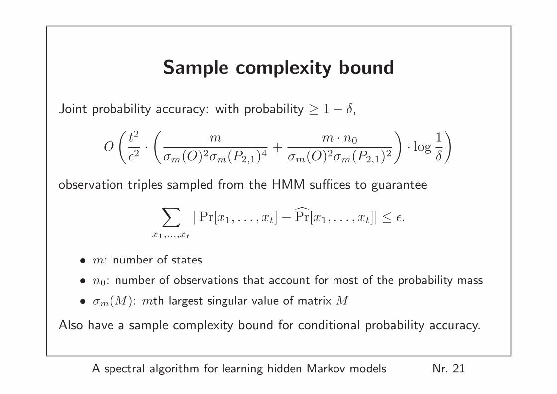
Sample complexity bound
Joint probability accuracy: with probability ≥ 1− δ,
O
(t2
ε2·(
m
σm(O)2σm(P2,1)4+
m · n0
σm(O)2σm(P2,1)2
)· log
1δ
)
observation triples sampled from the HMM suffices to guarantee
∑x1,...,xt
|Pr[x1, . . . , xt]− Pr[x1, . . . , xt]| ≤ ε.
• m: number of states
• n0: number of observations that account for most of the probability mass
• σm(M): mth largest singular value of matrix M
Also have a sample complexity bound for conditional probability accuracy.
A spectral algorithm for learning hidden Markov models Nr. 21
Conclusions and future work
Summary:
• Simple and efficient learning algorithm for invertible HMMs(sample complexity bounds, streaming implementation, etc.)
• Observable representation lets us avoid estimating T and O(n.b. could recover these if we really wanted, but less stable).
• SVD subspace captures dynamics of observable representation.
• Salvages old ideas and techniques from automata and control theory.
Future work:
• Improve efficiency, stability
• General linear dynamical models
• Behavior of EM under the rank condition?
A spectral algorithm for learning hidden Markov models Nr. 22
Thanks!
A spectral algorithm for learning hidden Markov models Nr. 23

Sample complexity bound
Conditional probability accuracy: with probability ≥ 1− δ,
poly(1/ε, 1/α, 1/γ, 1/σm(O), 1/σm(P2,1)) · (m2 + mn0) · log1δ
observation triples sampled from the HMM suffices to guarantee
KL(Pr[xt|x1:t−1]‖Pr[xt|x1:t−1]) ≤ ε
for all t and all history sequences x1:t−1.
• n0: number of observations that account for 1− ε of total probability mass,where ε = σm(O)σm(P2,1)ε/(4
√m)
• γ = inf~v:‖~v‖1=1 ‖O~v‖1 “value of observation” (Even-Dar et al, ’07)
• α = minx,i,j [Ax]ij (stochasticity requirement)
A spectral algorithm for learning hidden Markov models Nr. 24
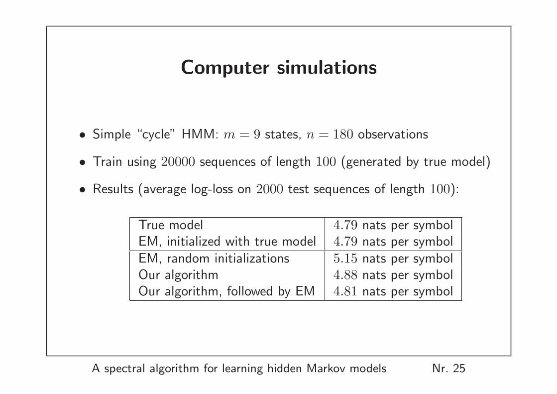
Computer simulations
• Simple “cycle” HMM: m = 9 states, n = 180 observations
• Train using 20000 sequences of length 100 (generated by true model)
• Results (average log-loss on 2000 test sequences of length 100):
True model 4.79 nats per symbolEM, initialized with true model 4.79 nats per symbolEM, random initializations 5.15 nats per symbolOur algorithm 4.88 nats per symbolOur algorithm, followed by EM 4.81 nats per symbol
A spectral algorithm for learning hidden Markov models Nr. 25