a speciﬁcation test for time series models by a normality

A Specification Test for Time Series Models by a Normality

Transformation

Jin-Chuan Duan∗

(First Draft: May 2003)(This Draft: Oct 2003)

Abstract

A correctly specified time series model can be used to transform data set into an i.i.d.sequence of standard normal random variables, assuming that the true parameter values areknown. In reality, however, one only has an estimated model and must therefore address thesampling errors associated with the parameter estimates. This paper presents a new test thatdoes not rely on specifying any specific alternative model. The test explores both normality andindependence of the transformed sequence. Specifically, we utilize the theoretical properties ofthe transformed residuals to construct a set of four test statistics, and for which the samplingerrors associated with any root-T consistent parameter estimates are eliminated. The size andpower of this new test are examined. We find the size of this test to be accurate for dynamicmodels such as AR, GARCH and diffusion. The power of this test is also good in the sense thatit can reject a mis-specified model using a reasonable sample size. The test is then applied toreal data series of stock returns and interest rates.

Key Words: Size, Power, GARCH, Diffusion, Asymptotic distribution

∗Duan is with Joseph L. Rotman School of Management, University of Toronto and is affiliated with CIRANO. E-mail: [email protected]; Tel: 416-946 5653; Fax: 416-971 3048. The author acknowledges support receivedas the Manulife Chair in Financial Services and research funding from both the Social Sciences and Humanities Re-search Council of Canada and the Natural Sciences and Engineering Research Council of Canada. The author thanksAndras Fulop for his programming assistance and benefits from the valuable comments by Haitao Li, Atsushi Inoueand the participants of the CIRANO-CIREQ financial econometrics conference in May, 2003 and the NBER/NSFTime Series Conference in September 2003.

1 Introduction

Time series models are used in econometrics and statistics to describe data set recorded over aperiod of time. The most pressing question is arguably about whether the given time series modelis a suitable specification for the data set. This paper provides a new test for addressing thisquestion. A time series model is a complete specification of the law governing the evolution of astochastic system that generates a data set recorded over time. It is quite common that the timeseries model uses a dynamic location-scale specification, meaning that the conditional mean andvariance are specified as functions of the previous variables but the distribution of the standardizedrandom variable is not. Examples of the dynamic location-scale model abound. The ARMA andGARCH models are such examples. There are also models that have a dependence structure beyondlocation and scale. A good example of this type is the mean-reverting square-root diffusion process(Feller process) that was adopted by Cox, et al (1985) to model interest rates. The conditionaldistribution over a discrete time period under this model is a non-central chi-square that cannot bereduced to a dynamic location-scale specification. For either case though, the assumed model hasa common feature that can be exploited in designing a specification test. As opposed to relyingon nesting the assumed model as is typically done, we propose in this paper a test that utilizesthe model specification as a transformation devise and examines the logical consequences of such atransformation.

The classical way of testing a distribution assumption without relying on specific alternativesis the Kolmogorov-Smirnov test or its variants such as the Andersen-Darling test. Such a testmeasures the distance between the theoretical distribution under the assumed model and the em-pirical distribution function. Different tests have different ways of measuring the distance with anintent to detect the departure from the assumed distribution in certain dimensions. For time seriesmodels, the distribution assumption does not completely characterize the system simply due to thepresence of dependence structure. The similar idea, nevertheless, applies. Diebold, et al (1998),Diebold, et al (1999), Bai (2002) and Hong and Li (2002) have proposed to transform the depen-dent data series using the conditional distribution function so as to obtain an i.i.d. sequence ofuniformly distributed transformed residuals. One can then proceed with the Kolmogorov type teston the transformed data set. Diebold, et al (1998) and Diebold, et al (1999) have not dealt withthe complex issue of parameter estimation uncertainty that inevitably accompanies the parameterestimate used in the conditional distribution function.1 Bai (2002) and Hong and Li (2002), onthe other hand, differ in their ways of dealing with parameter estimation uncertainty. Bai (2002)employs the Khmaladze (1981) martingale transformation to rid off the parameter estimation un-certainty. Hong and Li (2002) rely instead on a distance between a bivariate nonparametric kerneldensity estimate and the bivariate uniform density, which after normalization is not subject to theparameter estimation uncertainty.2

1The approach developed in Diebold, et al (1998) and Diebold, et al (1999) is more constructive in nature becausethe approach is meant to identify the correct conditional density function. Parameter estimation uncertainty is leftunaddressed, however.

2Bai’s (2002) test has not truly utilized the i.i.d. property of the transformed data set. In a way, it is similarto the Kolmogorov test that only tests the marginal distribution as opposed to the i.i.d. assumption. Hong and Li(2002), however, use the bivarate uniform distribution in constructing their test, which specifically takes into account

2

In the context of diffusion models, testing a specification without committing to a specific classof alternatives has also been studied. The first paper is, to our knowledge, Ait-Sahalia (1996a),in which the parametric density implied by the assumed diffusion model is compared to a densityestimated nonparametrically. Such an approach is innovative in the sense that the parameter valuesare estimated by minimizing the distance between two densities where only the parametric densitydepends on the model parameters. The minimum distance itself (after normalization) serve as a teststatistic to determine the adequacy of the assumed model. In other words, the parameter estimationand the test statistic are performed in one step. In contrast, the tests proposed by Bai (2002) andHong and Li (2002) are of the two-step nature. First, some

√T -consistent parameter estimate

is used to transform the data set. Then, one creates a test statistic that specifically exploresthe properties of the transformed residual.3 Although circumventing the parameter estimationuncertainty is desirable, it is not without costs; for example, it is not clear as to how one canmove from measuring the distance between two marginal densities as in Ait-Sahalia (1996a) tothat between two conditional densities without having obtained some parameter estimate first.4

Restricting to marginal densities will clearly weaken the power of test because the method does notseparate an i.i.d. data series from a dependent stationary series. As reported in Pritsker (1998),the Ait-Sahalia (1996a) test has a slow convergence rate for interest rate data, which results insignificant over-rejections even using a fairly large data sample, a result mainly attributable to thehigh persistence of the interest rate process. Relying on marginal densities (or distributions) hasanother drawback. As noted in Corradi and Swanson (2002), such a test cannot distinguish twodifferent models that share the same marginal density (or distribution).

The test proposed in this paper differs from the papers discussed thus far. Our test is constructedin three steps. First, we use the conditional distribution function under the assumed model totransform the time series of size T into an i.i.d. sequence of standard normal random variables. Inthis regard, the transformation is in spirit similar to Diebold, et al (1998), Diebold, et al (1999),Bai (2002) and Hong and Li (2002). Second, we partition the transformed residuals into manyindependent blocks of size n. Within each block of size n, we take advantage of normality to createa vector of n random variables, which is done by sequentially adding one variable at a time toa group of variables and then performing a nonlinear transformation. Third, the resulting i.i.d.sequence of n-dimensional random vectors is used to create a chi-square test statistic free of theroot-T consistent parameter estimation error. The creation of the n-dimensional random vectorvia the block structure is for the purpose of eliminating the parameter estimation error by lineartransformations. At the same time, the block structure allows the test statistic to exploit the

the i.i.d. feature of the transformed data set.3Thompson (2002) proposes a two-step method as well. The parameter estimation uncertainty is dealt with by

simulating the test statistic’s distribution using the asymptotic distribution of the√

T -consistent parameter estimate.Corradi and Swanson (2002) is another such kind of test being proposed in the literature. They use a shortertransformed series to construct the test statistic while relying on the parameter estimate from the longer data seriesas a way of “eliminating” the parameter estimation error. The cut-off value for the proposed test is then obtainedby the bootstrap technique.

4It should be noted that Ait-Sahalia (1996a) has also developed a way of utilizing conditional density informationthat measures “transition discrepancy” albeit such a test has not been empirically implemented in that paper. Theconditional version of the Ait-Sahalia (1996a) test is based on a theoretical observation that the time-derivative gapbetween the forward and backward equations for stationary diffusions should be zero.

3

independence nature of the transformed residuals under the assumed model. In this regard, thetest shares the spirit of Hong and Li (2002) in utilizing the independence property. The test is,however, completely parametric and relies on asymptotic inference. In this regard, it shares thesame feature of Bai’s (2002) test. Similar to the Bai (2002) and Hong and Li (2002), the cut-offvalue for testing is obtained from a known distribution. Thus, there is no need to perform computerintensive simulation or bootstrapping to determine the cut-off value as required by Thompson (2002)or Corradi and Swanson (2002).

It is worth noting that the proposed test does not require specifying an alternative class ofmodels to nest the assumed model. In this sense, the proposed testing method along with the onesdiscussed thus far extends the line of the Kolmogorov test. Thus, they are subject to the sameweakness and enjoy the similar benefit. A test without specifying a specific class of alternativesis expected to sacrifice some power of rejection, but it does not suffer the type-II error associatedwith specifying a wrong class of alternative models. Different ways of constructing specificationtests without alternatives are likely to have different powers of rejection. Intuitively though, thetest utilizing the independence structure of the transformed residuals can be expected to have ahigher power. In this sense, our proposed test is intuitively appealing.

This new test actually consists of four test statistics with an intent to examine four aspects ofthe transformed residual. We conduct a power analysis using two classes of models - AR-GARCHand diffusion. We use several special cases of the AR-GARCH model to generate data sets andtest the constant mean-variance and normality specification. The sizes of the four test statisticsare all found to be accurate for a sample size as small as 200. The power of the test is alsoquite satisfactory, and rejection occurs on different elements of the four test statistics as expectedand depending on which aspect of the generated data deviates from the assumed model. We alsogenerate three versions of the mean-reverting constant-elasticity-of-variance diffusion models tosimulate the interest rate data. We then study the size and power of testing the Vasicek (1977)specification for interest rates, which is one of the three versions used to generate the data sets.The sizes of the four test statistics are accurate for 500 data points (daily interest rates over twoyears), which is the smallest sample size studied for the diffusion model. For the sample size of2, 500 (daily interest rates over five years), the test has a moderate power of rejecting the Vasicek(1977) specification if the data set is generated by the Cox, et al (1985) model. In the case of theChan, et al (1992) specification, the power of rejecting the Vasicek (1977) model is very high.

We also apply the test to the real data of the S&P500 index returns (daily). The resultsindicate that the GARCH(1,1) model with conditional normality fails to pass the test for each oftwo subsamples but the GARCH(1,1) model with a conditional t-distribution only fails to pass forone of the two subsamples. When the test is applied to the Eurodollar deposit rate data (daily),we find that both the Vasicek (1977) and Cox, et al (1985) specifications are rejected resoundinglyfor all subsamples.

2 Specification test by a normality transformation

Consider a time series {Xt : t = 1, 2, · · · } and define Ft−1 to be the σ-field generated by {Xτ : τ ≤ t− 1}and all exogenous stochastic variables observable up to time t. Let Gt−1(Xt; θ) be the distribution

4

function of Xt, conditional on Ft−1, where θ denotes the model parameter(s). We maintain anassumption that Xt has a continuous conditional distribution function and is differentiable almosteverywhere.

For typical dynamic location-scale models, such as ARMA and GARCH, Gt−1(Xt; θ) is simpli-fied to some distribution function, say for example normal or student-t, and only the conditionalmean and standard deviation are used to reflect the dependence structure. For such cases, themodel is more commonly expressed as Xt = ft(µ) + vt(σ)εt, where ft(µ) and vt(σ) are measur-able with respect to Ft−1 and εt’s are random variables with mean 0, variance 1 and a commondistribution function with parameter η (or no additional parameter at all). Thus, θ = (µ, σ, η).This dynamic location-scale setup clearly encompasses typical time-series regression models withexogenous variables.

Our specification also includes the data series being sampled discretely from a diffusion model.For some diffusion model, such as the Ornstein-Uhlenbeck process that is commonly used to modelinterest rates, the discretely sampled data series is exactly governed by a dynamic location-scalemodel. For the mean-reverting square-root process (Feller process), on the other hand, the discretelysampled data series can no longer be described as a dynamic location-scale model. Nevertheless,the conditional distribution exists, and in particular, Gt−1(Xt; θ) is a non-central chi-square withthe non-centrality parameter depending on Xt−1. For more complex diffusion models, one mayneed to use a method such as the expansion idea of Ait-Sahalia (2002) to obtain an approximateclosed-form expression for Gt−1(Xt; θ).

Let kθ be the number of parameters in θ. Denote by θ̂T some√

T -consistent estimator for thetrue parameter value θ0. The standard normal distributional function is denoted by Φ(z). Define

ξt(θ) = Φ−1 [Gt−1 (Xt; θ)] . (1)

It is clear that ξt(θ0) forms an i.i.d. sequence of standard normal random variables, but ξt(θ) doesnot in general. We further transform ξt(θ) with the intention of eventually utilizing the fact thatξt(θ0)’s are i.i.d. standard normal random variables.5 Let

q(p)m,i(θ) =

m∑

j=1

ξp(i−1)∗m+j(θ) for p = 1, 2 (2)

q(3)m,i(θ) =

1m

m∑

j=1

ξ(i−1)∗m+j(θ)

2

(3)

q(4)m,i(θ) =

1m2

m∑

j=1

ξ2(i−1)∗m+j(θ)−m

2

. (4)

Use R(p)m (·) to denote the distribution function for q

(p)m,i(θ0). It is clear that R

(1)m (·) is a normal

distribution function with mean 0 and variance m. It is also clear that R(2)m (·) is the chi-square

5Transforming the observed variable into a standard normal random variable is not a theoretical necessity. Withoutthis normality transformation, however, we cannot take advantage of the analytical convenience associated withcombining normal random variables on which the test construction heavily depends.

5

distribution with m degrees of freedom. Similarly, R(3)m (·) is the chi-square distribution with 1

degree of freedom and R(4)m (x) = R

(2)m [m (1 +

√x)] − R

(2)m [m (1−√x)]. Note that R

(p)m (·) is not

model-specific.For an integer m ≥ 1 and i = 1, 2, · · · , [T/m], we define

Y(p)m,i(θ) = R(p)

m

(q(p)m,i(θ)

)− 1

2for p = 1, 2, 3, 4. (5)

Thus, Y(p)m,i(θ0) (for i = 1, 2, · · · ) forms an i.i.d. sequence of uniform (over

[−12 , 1

2

]) random variables

for any m ≥ 1 and p ∈ {1, 2, 3, 4}. Our set of test statistics is based on the following constructedvariables:

Z(p)m,T (θ) =

1√m[T/m]

[T/m]∑

i=1

Y(p)m,i(θ), for p = 1, 2, 3, 4. (6)

It is clear that√

TZ(p)m,T (θ0) converges to a normal random variable with mean 0 by the Central

Limit Theorem and the asymptotic variance can also be easily computed. Unfortunately, we do notknow θ0 and need to evaluate Z

(p)m,T (θ) at some parameter estimate θ̂T . Later, we devise the test

statistic corresponding to any given p, which relies on using some linear combinations of Z(p)m,T (θ̂T )

for different values of m to remove the sampling error associated with θ̂T .We now make a usual assumption about a

√T -consistent parameter estimator.

Assumption 1. The parameter estimator θ̂T for the time series {Xt : t = 1, 2, · · · } governed bythe conditional distribution function Gt−1(Xt; θ0) satisfies:

1.√

T(θ̂T − θ0

)= Op(1).

2.∂Z

(p)m,T (θ̂T )

∂θ′ converge in probability to a constant 1 × kθ vector for any finite m ≥ 1 andp = 1, 2, 3, 4.

By Assumption 1, we can apply the Taylor expansion to Z(p)m,T (θ̂T ) to obtain

√TZ

(p)m,T (θ̂T ) =

√TZ

(p)m,T (θ0) +

∂Z(p)m,T (θ0)

∂θ′√

T(θ̂T − θ0

)+ op(1). (7)

The term√

T(θ̂T − θ0

)does not vanish because it converges to a proper random vector as T ap-

proaches infinity. This√

T -consistent estimator carries with it a parameter estimation uncertainty.In order to have a test that has a correct size, one must address this parameter estimation uncer-tainty. The above Taylor expansion serves as the basis for us to construct a test statistic withoutsubjecting to the asymptotic distribution of the parameter estimate.

We now define a variance-covariance matrix of the limiting random variables, limT→∞

√TZ

(p)m,T (θ0)

for different m’s, which will be proved to be the case later in Theorem 1. Denote this matrix

6

corresponding to {m = 1, 2, · · · , n} by A(p)n×n and its (i, j)-element of this matrix is

a(p)ij =

√ij

κ(i, j)E

κ(i,j)/i∑

k=1

W(p)i,k

κ(i,j)/j∑

l=1

W(p)j,l

(8)

where

W(p)m,l = R(p)

m

m∑

j=1

εp(i−1)∗m+j

− 1

2for p = 1, 2 (9)

W(3)m,l = R(3)

m

1

m

m∑

j=1

ε(i−1)∗m+j

2− 1

2(10)

W(4)m,l = R(4)

m

1

m2

m∑

j=1

ε2(i−1)∗m+j −m

2− 1

2(11)

κ(i, j) is the lowest common multiple of i and j, and {εt; t = 1, 2, · · · } is an i.i.d. sequence ofstandard normal random variables. Note that A(p) does not depend on parameter value. Thediagonal elements of A(p) are always the same and can be computed analytically to yield a

(p)ii = 1

12for all i’s. The off-diagonal elements need to be assessed numerically and can, for example, becomputed by Monte Carlo simulation. Matrices A(p)

10×10 for p = 1, 2, 3 and 4 are presented inAppendix B for which one million simulation paths were used. These calculations need not berepeated because these matrices do not depend on a specific model.

The main result for the test statistic is stated in the following theorem.

Theorem 1. Assume that A(p)n×n is invertible and maintain Assumption 1. Let A(p)1/2

n×n denote itsCholesky decomposition (defined as a lower triangular matrix in this paper) and ‖·‖ be the

Euclidean norm. Let B(p)n×kθ

(θ0) consist of the limiting vectors∂Z

(p)m,T (θ̂T )

∂θ′ for m = 1, 2, · · · , n,

and r denote the column rank of B(p)n×kθ

(θ0). Then, for p ∈ {1, 2, 3, 4} and n > r, there exists

α(p)k×n that solves

α(p)k×nA

(p)−1/2n×n B(p)

n×kθ(θ0) = 0k×kθ

(12)

α(p)k×nα

(p)′k×n = Ik×k, (13)

and

J(p)T (θ̂T ) = T

∥∥∥∥∥∥∥∥α

(p)k×nA

(p)−1/2n×n

Z(p)1,T (θ̂T )

...Z

(p)n,T (θ̂T )

∥∥∥∥∥∥∥∥

2

D−→ χ2 (k) . (14)

where k = n− r.

7

Proof: see Appendix A

Although α(p) always exists, the solution is not unique. Non-uniqueness is due to rotations.A given solution can always be rotated by pre-multiplying α(p) with a unitary matrix. This non-uniqueness is inconsequential because the test statistic J

(p)T (θ̂T ) is invariant to the operation of

pre-multiplying by a unitary matrix. In other words, all solutions produce the same value for thetest statistic. To solve the system defined by equations (12) and (13), one can use the standardcomputer routine to find the orthonormal basis α(p) for the null space defined by equation (12); forexample, Matlab offers a procedure “Null” for this task.

Matrix B(p)n×kθ

(θ0) can be computed analytically in some cases. If, for example, the assumedmodel is a constant mean µ and variance σ2 with a normal distribution, then one can show that

for p = 1, limT→∞

∂Z(1)m,T (µ0,σ0)

∂µ = − 12σ0

√π

and limT→∞

∂Z(1)m,T (µ0,σ0)

∂σ = 0. Similarly for p = 2, we have

limT→∞

∂Z(2)m,T (µ0,σ0)

∂µ = 0 and limT→∞

∂Z(2)m,T (µ0,σ0)

∂σ = − 2√mσ0

∫∞0 z [h (z; m)]2 dz where h (·; m) is the chi-

square density function with m degrees of freedom. Unlike A(p), B(p)n×kθ

(θ0) is model-specific andis a function of the parameter. Since we do not know the true value, we need to use θ̂T instead.In other words, we use B(p)

n×kθ

(θ̂T

)in place of B(p)

n×kθ(θ0). In general, the analytical expression

for B(p)n×kθ

(θ0) may be too complex to derive, but can always be approximated by generating asimulated sample under the assumed model.

Before proceeding with finding the null space’s orthonormal basis, we need to recognize aproblem posed by the sampling error of B(p)

n×kθ

(θ̂T

). If a particular column of B(p)

n×kθ

(θ̂T

)is

theoretically linearly dependent on others, it might not be so numerically simply due to samplingerrors. In other words, we may have a theoretical rank that is less than kθ, but numerically itappears to have a rank equal to kθ. When the “genuine” rank is less than the rank in appearance,the null space will have a dimension less than its true dimension. Failing to find the “genuine”rank does not affect the size of test but may reduce its power. This is easily understood by anexample. Consider the case that n = 4, kθ = 3 and the true column rank equals 2, i.e., thereis one linearly dependent column in B(p)

4×3 (θ0). Due to sampling errors, its rank appears to be 3numerically, and thus the resulting null space has the dimension equal to 1. The orthonormal basisα(p) thus has only one row, but it could have two rows in the absence of sampling errors. Thedegrees of freedom of the test statistic rightly reflects the number of rows in α(p). The samplingerror has, however, unduly restricted the test statistic to be constructed in the one-dimensionalsubspace of the “genuine” two-dimensional null space. As a result, the power of the test may beadversely affected.

To address this issue, it is preferable to set a reasonable tolerance level so as to uncover the“genuine” rank by factoring in the approximate linear dependency. A reasonable tolerance levelmust take into account the sampling error for θ̂T . Consider, for example, a parameter with asmall sampling error. A small deviation from linear dependency may actually indicate a true linearindependence. In order to set a uniform tolerance level, we consider a system that is equivalent to

8

equations (12) and (13):

α(p)k×nA

(p)−1/2n×n B(p)

n×kθ

(θ̂T

)V1/2

kθ×kθ

(θ̂T

)= 0k×kθ

(15)

α(p)k×nα

(p)′k×n = Ik×k, (16)

where Vkθ×kθ

(θ̂T

)is the asymptotic variance-covariance matrix for

√T

(θ̂T − θ0

)under the as-

sumed model and the superscript 1/2 denotes its Cholesky decomposition (defined as a lower tri-angular matrix). The above system is motivated by the fact that the asymptotic variance-covariancematrix for

√TV−1/2

kθ×kθ

(θ̂T

)(θ̂T − θ0

)is an identity matrix. Note that A(p)−1/2

n×n B(p)n×kθ

(θ̂T

)V1/2

kθ×kθ

(θ̂T

)

is basically the multiplying matrix used to determine how much sampling errors of√TV−1/2

kθ×kθ

(θ̂T

)(θ̂T − θ0

)gets transmitted to the test statistic. Setting a tolerance level for

A(p)−1/2n×n B(p)

n×kθ

(θ̂T

)V1/2

kθ×kθ

(θ̂T

)amounts to applying a uniform maximum allowance level for

the sampling errors to impact the test statistic.Since we do not know whether the assumed model is the one that generates the data set, we

need to compute B(p)n×kθ

(θ̂T

)and Vkθ×kθ

(θ̂T

)directly by theory or approximate them numerically

using a simulated sample under the assumed model and the estimated parameter value θ̂T . Theresults reported in this paper are all based on using the simulated data to compute these twomatrices. The size of the simulated sample is set equal to the size of the original data sample tobe tested. Alternatively, one can avoid simulation by sticking to the original data set. Using theoriginal data set to compute these two matrices will not affect the size of the test, but it can affectthe power when the true model deviates from the assumed model.

We perform the singular-value decomposition on B(p)n×kθ

(θ̂T

)V1/2

kθ×kθ

(θ̂T

)to determine the

“genuine” rank of B(p)n×kθ

(θ̂T

). We set to zero all singular values that are smaller than 0.01 and

then reconstitute the matrix. The reconstituted matrix, denoted by P(p)n×kθ

, is approximately equal

to B(p)n×kθ

(θ̂T

)V1/2

kθ×kθ

(θ̂T

), and presumably carries with it the true rank of B(p)

n×kθ(θ0). We then

proceed to find the orthonormal basis α(p) for the null space defined by equations

α(p)k×nA

(p)−1/2n×n P(p)

n×kθ= 0k×kθ

(17)

α(p)k×nα

(p)′k×n = Ik×k. (18)

For the results presented later, we have chosen to fix the degrees of freedom to a particular valueof k as opposed to setting n. This can be easily accomplished using the following procedure. Firstwe tentatively set n = kθ + k, and then check the dimension of the null space. If it equals k, thenstop. Otherwise, we reduce n by 1 and repeat the same check. It is not difficult to see that thisprocedure guarantees the dimension of the final null space equal to k.

9

3 Power analysis

The four statistics (p = 1, 2, 3 and 4) test different dimensions of the model specification. For p = 1and 2, we examine the transformed residuals (i.i.d. standard normally distributed residuals underthe assumed model) to see whether their mean and variance are correctly specified. The test statisticfor p = 3 checks to see whether the transformed residuals are autocorrelated. In the case of p = 4,we test whether the squared transformed residuals are autocorrelated. In an intuitive way, the fourtest statistics offer more than just a formal statistical statement of rejection/no rejection. Theyactually reveal the nature of model misspecification. For example, when a data set generated by asymmetric fat-tailed distribution is mistakenly modeled as a normal distribution, the transformedresidual is effectively “stretched” so that its variance becomes larger than the predicted value underthe assumed model. Similarly, if a data set generated by a symmetric distribution is erroneouslymodeled as an asymmetric distribution, the transformed residual will have a mean distorted awayfrom the value predicted by the assumed model.

In this section, we conduct a power analysis using two popular classes of models: AR-GARCHand diffusion models. Two specific null hypotheses are tested with various alternative models usedto generate the data sets. In all cases, we set the degrees of freedom of the test statistic to 2 andtabulate the rejection rate using 500 simulations.

3.1 AR-GARCH models

Consider the following model:

Xt = µ + γXt−1 + σtεt (19)σ2

t = β0 + β1σ2t−1 + β2σ

2t−1ε

2t−1 (20)

where εt’s are i.i.d. mean 0 and variance 1 continuous random variables with a t-distributionfunction of η degrees of freedom. For the power analysis, we test special cases of this modelwithout assuming the knowledge that the above model is used to generate the data set. A model tobe tested has the relevant parameter θ that is a subset of (µ, γ, β0, β1, β2, η). In order to computethe test statistic, we only need to estimate the restricted model. Specifically, we use the maximumlikelihood estimator θ̂T for the restricted model.

Case 1: The assumed model: constant mean and variance with normality, i.e., γ = 0,β1 = 0, β2 = 0 and η = ∞.

Under the assumed model, we have θ = {µ, σ} where σ =√

β0. We can use the sample mean andstandard deviation of {X1, X2, · · · , XT }. We consider all four test statistics: J

(p)T (θ̂T ), p = 1, 2, 3, 4

and study the size and power for each of them.We set the stationary mean and variance to 0 and 1, respectively, in generating the data sets.

For the power analysis we alter the value for γ, β2 and η individually. When γ 6= 0, it is theconstant mean assumption being violated. Similarly, 1/η 6= 0 implies a violation of normality. Inthe power analysis with respect to γ, we control for both the level and volatility of the process.Specifically, we keep µ/(1 − γ) and σ2/(1 − γ2) constant where the two formulas are well known

10

results for the AR(1) model. For the power analysis of stochastic volatility, i.e., varying β2, we setout to maintain the same overall level of volatility when generating the ARCH(1) model. If thevalue of β0 is fixed, an increase in β2 will not only generate stochastic volatility but also cause theoverall level of volatility to rise. To control for the volatility level, we set σ̄2 = 1 and maintainβ0 = σ̄2 (1− β1 − β2) when the value β2 is varied.6 In generating data, we also set σ2

1 = σ̄2,meaning that the initial data point has the average volatility.

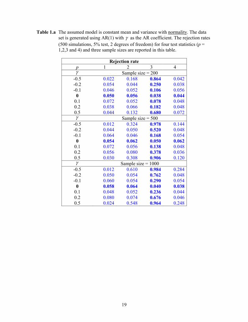
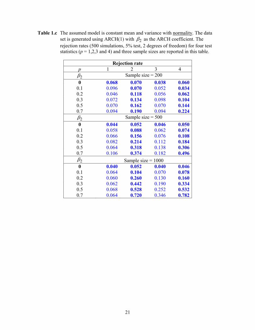
Tables 1.a-1.c present the rejection rates (5% test, 2 degrees of freedom) for various parametervalues and three sample sizes (200, 500 and 1000). The size in all cases are fairly accurate. Whenthe data generating model is the AR(1) process, the assumed model (normality with constant meanand variance) is rejected mainly for p = 3 (Table 1.a). This result is hardly surprising because thetransformed residuals should be autocorrelated. If the data is generated by a t-distribution, wehave strong rejection for p = 2 (Table 1.b). As discussed in the beginning of Section 3, we expectrejection under p = 2 for this case. This is true because the transformed residual is effectively“stretched” so that its variance becomes larger than the predicted value under the assumed model.Finally in Table 1.c, we see rejection under p = 2 and 4 when the data set is generated usingthe ARCH(1) model. Having rejection under p = 4 is completely expected because the squaredtransformed residuals are autocorrelated. As to rejection under p = 2, the reason is similar to thecase of t-distributed data. The ARCH(1) model with conditional normality makes the marginaldistribution exhibit a fat-tailed feature, and as a result, produces the “stretching” effect.

3.2 Diffusion models

We limit our power study to the class of mean-reverting constant-elasticity-of-variance diffusionmodels:

dXt = κ(µ−Xt)dt + σXδt dWt (21)

where Wt is a Wiener process. We simulate the data set by approximating the above diffusion modelwith 20 subintervals within one recording data interval. In other words, we record once every 20simulated data points to mimic a discretely sampled data set under the diffusion assumption. TheMilstein scheme is used to generate the data set.

The assumed model is the Ornstein and Uhlenbeck process, a special case of equation (21) bysetting δ = 0. The parameters of this model can be estimated by maximum likelihood or other

√T -

consistent estimation methods like GMM. The results presented below are based on the maximumlikelihood estimates.

Three special versions of the diffusion model in equation (21) are used to generate the data fortesting. The first model is the Ornstein-Uhlenbeck process, i.e., δ = 0. Its use for modeling interestrates was popularized by Vasicek (1977) in which this process plays a pivotal role in deriving theVasicek bond pricing model. For ease of discussion, we refer to it as the Vasicek model. Next, weuse the mean-reversion square-root diffusion (Feller process), i.e., δ = 1/2. This process was usedby Cox, Ingersoll and Ross (1985) to obtain the well-known CIR bond pricing model. Again forease of discussion, we refer to it as the CIR model. Finally, the version established in Chan, et al(1992) is referred to as the CKLS model, which reports an estimate of δ equal to 1.4999.

6This is due to the fact that the stationary volatility equals σ̄2 = β0/ (1− β1 − β2)

11

Case 2: The assumed model: the Vasicek model, i.e., δ = 0.The data sets used in the power analysis are generated by three different models. First, we gener-

ate the Vasicek model using the following set of parameter values: (κ, µ, σ2) = (0.85837, 0.089102,0.002185), which was used in Pritsker (1998) and was in turn taken from Ait-Sahalia (1996b).The second model is the CIR model with the following set of parameter values: (κ, µ, σ2) =(0.89218, 0.090495, 0.032742). Again they were used in Pritsker (1998) and Ait-Sahalia (1996b).These two sets of parameter values are based on the unit of time being one year. For the dailyfrequency, we thus divide both κ and σ2 by 252. The final model is the CKLS specification with theother parameter values reported in Chan, et al (1992): (κ, µ, σ2) = (0.5921, 0.0689, 1.6704). Theseparameter values correspond to one month as the basic unit of time. Thus, we divide both κ andσ2 by 21.

Table 2 indicates that the size of test (for p = 1, 2, 3 and 4) is correct for the sample size assmall as 500, a sample size that is roughly equal to daily observations over two years. This resultstands in sharp contrast to that of the Ait-Sahalia test as discussed in Pristker (1998), where heargues that the Ait-Sahalia test needs to have an exceedingly large sample of interest rate data inorder to have a right size.

The power of rejecting the Vasicek model mainly resides with the test under p = 4, which checksto see whether the squared transformed residuals are autocorrelated. Assuming the Vasicek modelwhile the data is generated by the CIR model induces autocorrelation in the conditional variancebecause these two models only differ in how the diffusion term is specified. A similar argumentapplies to the data set generated by the CKLS model.7 In order to have a moderate power (50%) ofrejecting the Vasicek model when the data is generated by the CIR model, one needs to have about10 years worth of daily interest rate data. It is, however, much easier to reject the Vasicek model(in excess of 90%) if the data is generated by the CKLS model, a result that is hardly surprising.

4 Application to real data

Two real data series are now considered. The first series is the daily S&P500 index returns (totalreturn index from April 16, 1993 to April 16, 2003, continuously compounded) extracted fromDatastream whereas the second series is the 7-day Eurodollar deposit spot rates on a daily frequencyfrom June 1, 1973 to February 25, 1995, a data set used in Ait-Sahalia (1996a). We present theparameter estimates under the assumed models as well as the testing results using the four teststatistics for each of the assumed models. Similar to the power analysis, we set the degrees offreedom of the test statistic to 2.

7When the data set is generated by the CKLS model, the power of test (p = 4) does not necessarily increase withthe sample size. For example, it drops from 76.8% to 41.4% when the sample size is increased from 500 to 1, 000.This result is due to sometimes obtaining the AR(1) coefficient estimate greater than 1 when the sample size equals

500. It leads to an explosive B(p)n×kθ

�θ̂T

�and thus a rejection.

12

4.1 S&P500 index returns

The equity market index return is commonly modeled by the GARCH model in the empirical financeliterature. For the S&P500 index return series, we consider two cases under the GARCH model.The results for the whole sample (2520 data points) and two subsamples (938 and 1582 data points)are provided. The whole sample is divided on December 31, 1996, because inspection of the returntime series plot reveals a clear structural break. The maximum likelihood parameter estimates areused to compute the test statistics. The parameter estimates obtained for this model, reported inthe bottom panel of Table 3.a, are similar to the typical results reported in the literature.

The first model applied to the S&P500 index return series is the linear GARCH(1,1) modelwith a conditional normal distribution. The results are presented in Table 3.a. The model is notrejected (at the 5% significance level) using the whole data sample but rejected for either subsample.Rejection takes place either with p = 2 or 4, meaning that the transformed residual has a variancedifferent from the one predicted by the assumed model or the squared transformed residuals areautocorrelated. Given the extensive evidence supporting conditional leptokurtosis in the empiricalfinance literature, rejection (p = 2) for the second subsample is expected. For the first subsample,rejection (p = 4) suggests that the GARCH(1,1) variance dynamic is likely misspecified. Whatis surprising is our failure to reject the GARCH(1,1)-normality model using the whole sample.Perhaps, the structural break has mixed together two different kinds of misspecification present inthe two subsamples.

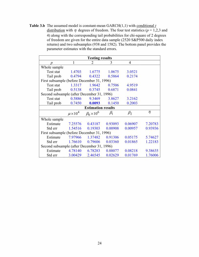
The second model considered for the S&P500 index return series is the GARCH(1,1) modelwith a conditional t-distribution and the results are presented in Table 3.b. One can view thismodel as a natural progression from the GARCH model with conditional normality. We can stillreject the model at the 5% level for the second subsample, and rejection continues to occur withp = 2, indicating the transformed residual still has a variance different from that predicted by theassumed model. Since the assumed model has allowed for leptokurtosis, rejection may indicate aproblem with using t-distribution to model the data in the second subsample.

4.2 Eurodollar deposit rates

Arguably the most popular models used for describing interest rates are two specific diffusionmodels that we considered in Section 3.2: the Vasicek and CIR models. Their popularity has muchto do with the fact that both models yield a bond pricing model that is exponential-affine andanalytically convenient. We now study their performance in describing the Eurodollar deposit rateseries. We run the four tests for the whole series with 5, 505 data points as well as five subsamplesof 1, 000 data points for both models.

The results for the Vasicek model are presented in Table 4.a. Since the Vasicek model for thediscretely sampled data set is effectively an AR(1) model, we simply use the lagged regression toobtain the simplest

√T -consistent estimates. Each of the parameter values can be converted to

the parameter values under the Vasicek model. Note that κ and σ are stated in terms of the unitof time equal to one year. The test results (p = 2 and 4) clearly indicate that the Vasicek modelperforms poorly. These resounding rejections suggest that the transformed residual does not havethe right variance and the squared transformed residuals are autocorrelated. The fact that rejection

13

consistently falls on p = 2 and 4 for the whole sample as well as for the five subsamples indicatesa persistent pattern of misspecification.

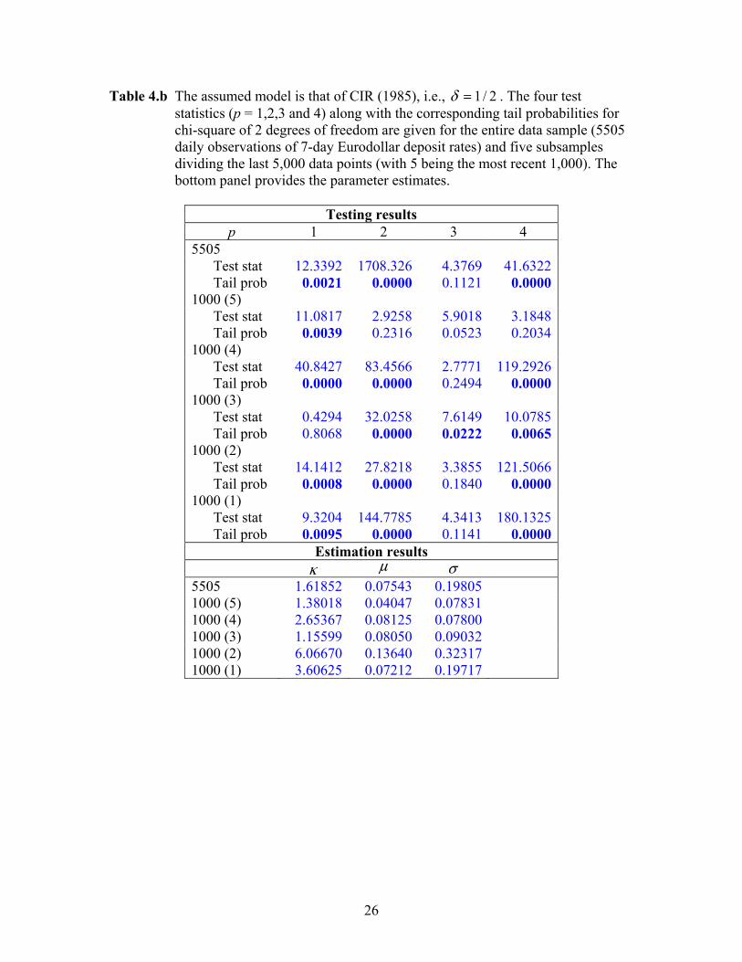
Table 4.b present the results of testing the CIR model. Contrary to a common belief, this modelperforms no better than the Vasicek model. It has been resoundingly rejected for all p = 2 and 4except for the most recent 1, 000 data points. In addition, the mean of the transformed residualalso differs from the model prediction. This result is interesting given that the mean-revertingspecification presumably allows for the mean of the interest rate series to be freely located andshould thus exhibit no level bias. The conditional density function under the assumed model has,however, distorted the mean of the transformed residual. The result clearly points to the wrongskewed distribution (non-central chi-square) implied by the CIR model.

A Proof of Theorem 1

First, we argue that there exists a solution α(p)k×n. Because the column rank of A(p)−1/2

n×n B(p)n×kθ

(θ0)is r, the null space has a dimension equal to k = n− r. Therefore, there will always be a solutionα

(p)k×n to equations (12) and (13).

Next, we use Assumption 1 and the Taylor expansion in equation (7) to compute

√Tα

(p)k×nA

(p)−1/2n×n

Z(p)1,T (θ̂T )

...Z

(p)n,T (θ̂T )

= α(p)k×nA

(p)−1/2n×n

√TZ

(p)1,T (θ0)...√

TZ(p)n,T (θ0)

+ α

(p)k×nA

(p)−1/2n×n

∂Z(p)1,T (θ0)

∂θ′...

∂Z(p)n,T (θ0)

∂θ′

√

T(θ̂T − θ0

)+ op(1)

= α(p)k×nA

(p)−1/2n×n

√TZ

(p)1,T (θ0)...√

TZ(p)n,T (θ0)

+ α

(p)k×nA

(p)−1/2n×n B(p)

n×kθ(θ0)

√T

(θ̂T − θ0

)+ op(1)

= α(p)k×nA

(p)−1/2n×n

√TZ

(p)1,T (θ0)...√

TZ(p)n,T (θ0)

+ op(1).

Let n∗ be the lowest common multiple of {1, 2 · · · , n}. For any 1 ≤ m ≤ n,

14

√TZ

(p)m,T (θ0) =

√T/m

[T/m]

[T/m]∑

i=1

Y(p)m,i(θ0)

=1√T/m

[T/n∗]∑

l=1

n∗/m∑

j=1

Y(p)

m,(l−1)n∗m

+j(θ0) + op(1)

=1√

T/n∗

[T/n∗]∑

l=1

√m

n∗

n∗/m∑

j=1

Y(p)

m,(l−1)n∗m

+j(θ0)

+ op(1)

=1√

T/n∗

[T/n∗]∑

l=1

Hl(p, m) + op(1)

where

Hl(p,m) =√

m

n∗

n∗/m∑

j=1

Y(p)

m,(l−1)n∗m

+j(θ0).

Thus,

α(p)k×nA

(p)−1/2n×n

√TZ

(p)1,T (θ0)...√

TZ(p)n,T (θ0)

=

1√T/n∗

[T/n∗]∑

l=1

α

(p)k×nA

(p)−1/2n×n

Hl(p, 1)...

Hl(p, n)

+ op(1)

=1√

T/n∗

[T/n∗]∑

l=1

Ql(p) + op(1)

where

Ql(p) = α(p)k×nA

(p)−1/2n×n

Hl(p, 1)...

Hl(p, n)

.

Note that Ql(p)’s form an i.i.d. sequence of k-dimensional random vectors with mean 0k×1 andvariance covariance matrix Ik×k. This is true because (1) Y

(p)m,j(θ0) has a zero mean, and (2)

E(∑n∗/i

k=1 Y(p)i,k (θ0)

∑n∗/jl=1 Y

(p)j,l (θ0)

)= a

(p)ij with a

(p)ij being defined in equation (8). The second fact

can be established by decomposing the n∗-element block into n∗/κ(i, j) independent blocks withκ(i, j) elements each so that

E

n∗/i∑

k=1

Y(p)i,k (θ0)

n∗/j∑

l=1

Y(p)j,l (θ0)

= E

n∗/i∑

k=1

W(p)i,k

n∗/j∑

l=1

W(p)j,l

=√

ij

κ(i, j)E

κ(i,j)/i∑

k=1

W(p)i,k

κ(i,j)/j∑

l=1

W(p)j,l

.

15

Applying the Central Limit Theorem yields

α(p)k×nA

(p)−1/2n×n

√TZ

(p)1,T (θ0)...√

TZ(p)n,T (θ0)

D−→ N (0, Ik×k) .

Thus,J

(p)T (θ̂T ) D−→ χ2 (k) .

The proof is thus complete.

B Expression for matrix A(p)

The following 10× 10 matrices are computed using Monte Carlo simulation with one million repe-titions.

A(1)10×10 =

0.0833 0.0813 0.0808 0.0806 0.0803 0.0801 0.0801 0.0799 0.0800 0.08000.0813 0.0834 0.0814 0.0813 0.0808 0.0808 0.0806 0.0804 0.0802 0.08030.0808 0.0814 0.0833 0.0812 0.0810 0.0814 0.0808 0.0806 0.0807 0.08060.0806 0.0813 0.0812 0.0834 0.0814 0.0815 0.0810 0.0812 0.0806 0.08080.0803 0.0808 0.0810 0.0814 0.0833 0.0814 0.0816 0.0810 0.0808 0.08140.0801 0.0808 0.0814 0.0815 0.0814 0.0834 0.0814 0.0813 0.0813 0.08120.0801 0.0806 0.0808 0.0810 0.0816 0.0814 0.0834 0.0816 0.0813 0.08120.0799 0.0804 0.0806 0.0812 0.0810 0.0813 0.0816 0.0834 0.0816 0.08150.0800 0.0802 0.0807 0.0806 0.0808 0.0813 0.0813 0.0816 0.0833 0.08130.0800 0.0803 0.0806 0.0808 0.0814 0.0812 0.0812 0.0815 0.0813 0.0834

A(2)10×10 =

0.0833 0.0766 0.0730 0.0707 0.0692 0.0683 0.0676 0.0670 0.0666 0.06640.0766 0.0833 0.0792 0.0785 0.0767 0.0762 0.0751 0.0749 0.0744 0.07400.0730 0.0792 0.0834 0.0799 0.0793 0.0794 0.0782 0.0778 0.0776 0.07680.0707 0.0785 0.0799 0.0832 0.0802 0.0802 0.0796 0.0800 0.0788 0.07860.0692 0.0767 0.0793 0.0802 0.0833 0.0803 0.0803 0.0800 0.0797 0.08010.0683 0.0762 0.0794 0.0802 0.0803 0.0834 0.0807 0.0805 0.0806 0.07990.0676 0.0751 0.0782 0.0796 0.0803 0.0807 0.0833 0.0807 0.0806 0.08060.0670 0.0749 0.0778 0.0800 0.0800 0.0805 0.0807 0.0834 0.0806 0.08090.0666 0.0744 0.0776 0.0788 0.0797 0.0806 0.0806 0.0806 0.0832 0.08080.0664 0.0740 0.0768 0.0786 0.0801 0.0799 0.0806 0.0809 0.0808 0.0833

16

A(3)10×10 =

0.0833 0.0434 0.0331 0.0278 0.0243 0.0218 0.0202 0.0188 0.0175 0.01660.0434 0.0833 0.0436 0.0434 0.0330 0.0330 0.0277 0.0277 0.0244 0.02440.0331 0.0436 0.0833 0.0437 0.0393 0.0434 0.0333 0.0313 0.0330 0.02800.0278 0.0434 0.0437 0.0833 0.0437 0.0433 0.0380 0.0435 0.0337 0.03310.0243 0.0330 0.0393 0.0437 0.0833 0.0438 0.0414 0.0389 0.0373 0.04350.0218 0.0330 0.0434 0.0433 0.0438 0.0834 0.0440 0.0437 0.0435 0.03950.0202 0.0277 0.0333 0.0380 0.0414 0.0440 0.0833 0.0437 0.0422 0.04070.0188 0.0277 0.0313 0.0435 0.0389 0.0437 0.0437 0.0832 0.0441 0.04370.0175 0.0244 0.0330 0.0337 0.0373 0.0435 0.0422 0.0441 0.0834 0.04390.0166 0.0244 0.0280 0.0331 0.0435 0.0395 0.0407 0.0437 0.0439 0.0834

A(4)10×10 =

0.0841 0.0485 0.0311 0.0229 0.0186 0.0160 0.0141 0.0127 0.0120 0.01090.0485 0.0833 0.0538 0.0461 0.0351 0.0316 0.0267 0.0249 0.0222 0.02100.0311 0.0538 0.0831 0.0536 0.0462 0.0455 0.0359 0.0326 0.0321 0.02770.0229 0.0461 0.0536 0.0832 0.0528 0.0499 0.0427 0.0449 0.0359 0.03400.0186 0.0351 0.0462 0.0528 0.0839 0.0521 0.0481 0.0443 0.0412 0.04450.0160 0.0316 0.0455 0.0499 0.0521 0.0835 0.0508 0.0495 0.0481 0.04310.0141 0.0267 0.0359 0.0427 0.0481 0.0508 0.0826 0.0500 0.0479 0.04520.0127 0.0249 0.0326 0.0449 0.0443 0.0495 0.0500 0.0827 0.0500 0.04860.0120 0.0222 0.0321 0.0359 0.0412 0.0481 0.0479 0.0500 0.0832 0.04900.0109 0.0210 0.0277 0.0340 0.0445 0.0431 0.0452 0.0486 0.0490 0.0823

References

[1] Ait-Sahalia, Y., 1996a, Testing Continuous-Time Models of the Spot Interest Rate, Review ofFinancial Studies 9, 385-426.

[2] Ait-Sahalia, Y., 1996b, Nonparametric Pricing of Interest Rate Derivative Securities, Econo-metrica 64, 527-560.

[3] Ait-Sahalia, Y., 2002, Maximum-Likelihood Estimation of Discretely Sampled Diffusions: AClosed-Form Approach, Econometrica 70, 223-262.

[4] Bai, J., 2002, Testing Parametric Conditional Distributions of Dynamic Models, unpublishedmanuscript, Boston College.

[5] Bontemps, C. and N. Meddahi, 2002, Testing Normality: A GMM Approach, unpublishedmanuscript, CIRANO.

[6] Chan, K., A. Karolyi, F. Longstaff and A. Sanders, 1992, An Empirical Comparison of Alter-native Models of the Short-Term Interest Rate, Journal of Finance 47, 1209-1227.

17

[7] Corradi, V. and N. Swanson, 2002, A Bootstrap Specification Test for Diffusion Processes,unpublished manuscript, University of Exeter.

[8] Cox, J., J. Ingersoll and S. Ross, 1985, A Theory of the Term Structure of Interest Rates,Econometrica 53, 385-407.

[9] Diebold, F., T. Gunther and A. Tay, 1998, Evaluating Density Forecasts with Applications toFinancial Risk Management, International Economic Review 39, 863-883.

[10] Diebold, F., J. Hahn and A. Tay, 1999, Multivariate Density Forcast Evaluation and Calibra-tion in Financial Risk Management: High-Frequency Returns on Foreign Exchange, Review ofEconomics and Statistics 81, 661-673.

[11] Hong, Y. and H. Li, 2002, Nonparametric Specification Testing for Continuous-Time Modelswith Applications to Spot Interest Rates, unpublished manuscript, Cornell University.

[12] Khmaladze, E., 1981, Martingale Approach in the Theory of Goodness-of-Fit Tests, Theoryof Probability and its Applications 26, 240-257.

[13] Thompson, S., 2002, Specification Tests for Continuous Time Models, unpublished manuscript,Harvard University.

[14] Vasicek, O., 1977, An Equilibrium Characterization of the Term Structure, Journal of Finan-cial Economics 5, 177-188.

18

19

Table 1.a The assumed model is constant mean and variance with normality. The data set is generated using AR(1) with γ as the AR coefficient. The rejection rates (500 simulations, 5% test, 2 degrees of freedom) for four test statistics (p = 1,2,3 and 4) and three sample sizes are reported in this table.

Rejection rate

p 1 2 3 4 γ Sample size = 200

-0.5 0.022 0.168 0.864 0.042 -0.2 0.054 0.044 0.250 0.038 -0.1 0.046 0.052 0.106 0.056

0 0.050 0.056 0.038 0.044 0.1 0.072 0.052 0.078 0.048 0.2 0.038 0.066 0.182 0.048 0.5 0.044 0.132 0.680 0.072 γ Sample size = 500

-0.5 0.012 0.324 0.978 0.144 -0.2 0.044 0.050 0.520 0.048 -0.1 0.064 0.046 0.168 0.054

0 0.054 0.062 0.050 0.062 0.1 0.072 0.056 0.138 0.048 0.2 0.056 0.080 0.378 0.036 0.5 0.030 0.308 0.906 0.120 γ Sample size = 1000

-0.5 0.012 0.610 0.984 0.284 -0.2 0.050 0.054 0.762 0.048 -0.1 0.060 0.054 0.290 0.054

0 0.058 0.064 0.040 0.038 0.1 0.048 0.052 0.236 0.044 0.2 0.080 0.074 0.676 0.046 0.5 0.024 0.548 0.964 0.248

20

Table 1.b The assumed model is constant mean and variance with normality. The data set is generated using t-distribution with η as the degrees of freedom. The rejection rates (500 simulations, 5% test, 2 degrees of freedom) for four test statistics (p = 1,2,3 and 4) and three sample sizes are reported in this table.

Rejection rate

p 1 2 3 4 η Sample size = 200 ∞ 0.068 0.056 0.044 0.050 20 0.060 0.090 0.052 0.032 10 0.066 0.088 0.048 0.066 7 0.094 0.140 0.062 0.064 5 0.070 0.308 0.050 0.150 4 0.076 0.438 0.094 0.228 η Sample size = 500 ∞ 0.052 0.050 0.046 0.052 20 0.054 0.088 0.060 0.060 10 0.062 0.166 0.064 0.096 7 0.088 0.306 0.076 0.146 5 0.070 0.524 0.150 0.256 4 0.070 0.708 0.192 0.450 η Sample size = 1000 ∞ 0.062 0.044 0.038 0.042 20 0.070 0.110 0.066 0.060 10 0.058 0.212 0.070 0.114 7 0.064 0.490 0.146 0.204 5 0.054 0.750 0.264 0.404 4 0.054 0.874 0.402 0.574

21

Table 1.c The assumed model is constant mean and variance with normality. The data set is generated using ARCH(1) with 2β as the ARCH coefficient. The rejection rates (500 simulations, 5% test, 2 degrees of freedom) for four test statistics (p = 1,2,3 and 4) and three sample sizes are reported in this table.

Rejection rate

p 1 2 3 4 2β Sample size = 200

0 0.068 0.070 0.038 0.060 0.1 0.096 0.070 0.052 0.034 0.2 0.046 0.118 0.056 0.062 0.3 0.072 0.134 0.098 0.104 0.5 0.070 0.162 0.070 0.144 0.7 0.094 0.190 0.094 0.224

2β Sample size = 500 0 0.044 0.052 0.046 0.050

0.1 0.058 0.088 0.062 0.074 0.2 0.066 0.156 0.076 0.108 0.3 0.082 0.214 0.112 0.184 0.5 0.064 0.318 0.138 0.306 0.7 0.106 0.374 0.182 0.496

2β Sample size = 1000 0 0.040 0.052 0.040 0.046

0.1 0.064 0.104 0.070 0.078 0.2 0.060 0.260 0.130 0.160 0.3 0.062 0.442 0.190 0.334 0.5 0.068 0.528 0.252 0.532 0.7 0.064 0.720 0.346 0.782

22

Table 2 The assumed model is that of Vasicek (1977). The data set are generated using the Vasicek, CIR and CKLS specifications. The rejection rates (500 simulations, 5% test, 2 degrees of freedom) for four test statistics (p = 1,2,3 and 4) and four sample sizes are reported in this table.

Rejection rate

p 1 2 3 4 Generating

model Sample size = 500

Vacicek 0.068 0.064 0.056 0.054 CIR 0.068 0.068 0.052 0.086

CKLS 0.084 0.080 0.028 0.768 Sample size = 1000

Vacicek 0.054 0.058 0.058 0.056 CIR 0.058 0.056 0.050 0.106

CKLS 0.070 0.372 0.030 0.414 Sample size = 2500

Vacicek 0.048 0.042 0.046 0.052 CIR 0.044 0.080 0.050 0.510

CKLS 0.046 0.846 0.022 0.938 Sample size = 5500

Vacicek 0.062 0.054 0.060 0.040 CIR 0.072 0.088 0.054 0.910

CKLS 0.054 0.844 0.020 1.000

23

Table 3.a The assumed model is constant-mean GARCH(1,1) with conditional normality. The four test statistics (p = 1,2,3 and 4) along with the corresponding tail probabilities for chi-square of 2 degrees of freedom are given for the entire data sample (2520 S&P500 daily index returns) and two subsamples (938 and 1582). The bottom panel provides the parameter estimates with the standard errors.

Testing results

p 1 2 3 4 Whole sample

Test stat 0.8966 3.7121 1.7936 4.4100 Tail prob 0.6387 0.1563 0.4079 0.1102

First subsample (before December 31, 1996) Test stat 0.6285 4.3924 0.5948 7.6292 Tail prob 0.7303 0.1112 0.7427 0.0220

Second subsample (after December 31, 1996) Test stat 0.7196 8.3280 4.9996 1.2520 Tail prob 0.6978 0.0155 0.0821 0.5347

Estimation results 410×µ 6

0 10×β 1β 2β

Whole sample Estimate 6.74237 0.62628 0.91879 0.08044 Std err 1.64537 0.16021 0.00684 0.00679

First subsample (before December 31, 1996) Estimate 7.26237 1.20327 0.91697 0.05122 Std err 1.92170 0.42218 0.01940 0.01143

Second subsample (after December 31, 1996) Estimate 5.06697 9.47883 0.84799 0.10085 Std err 3.18199 2.14413 0.02140 0.01379

24

Table 3.b The assumed model is constant-mean GARCH(1,1) with conditional t distribution with η degrees of freedom. The four test statistics (p = 1,2,3 and 4) along with the corresponding tail probabilities for chi-square of 2 degrees of freedom are given for the entire data sample (2520 S&P500 daily index returns) and two subsamples (938 and 1582). The bottom panel provides the parameter estimates with the standard errors.

Testing results

p 1 2 3 4 Whole sample


First subsample (before December 31, 1996) Test stat 1.3317 1.9642 0.7506 4.9519 Tail prob 0.5138 0.3745 0.6871 0.0841

Second subsample (after December 31, 1996) Test stat 0.5886 9.3469 3.8627 3.2162 Tail prob 0.7450 0.0093 0.1450 0.2003

Estimation results 410×µ 6

0 10×β 1β 2β η

Whole sample Estimate 7.25576 0.43187 0.93093 0.06907 7.20783 Std err 1.54516 0.19303 0.00908 0.00957 0.93936

First subsample (before December 31, 1996) Estimate 7.97966 1.37482 0.91306 0.05175 5.74627 Std err 1.76610 0.79606 0.03360 0.01865 1.22183

Second subsample (after December 31, 1996) Estimate 4.78140 6.78283 0.88077 0.08218 9.38635 Std err 3.00429 2.46545 0.02629 0.01769 1.76006

25

Table 4.a The assumed model is that of Vasicek (1977), i.e., 0=δ . The four test statistics (p = 1,2,3 and 4) along with the corresponding tail probabilities for chi-square of 2 degrees of freedom are given for the entire data sample (5505 daily observations of 7-day Eurodollar deposit rates) and five subsamples dividing the last 5,000 data points (with 5 being the most recent 1,000). The bottom panel provides the parameter estimates.

Testing results

p 1 2 3 4 5505


1000 (5) Test stat 1.6580 9.8752 2.3462 30.2330 Tail prob 0.4365 0.0072 0.3094 0.0000





Estimation results κ µ σ 5505 1.60884 0.08308 0.06460 1000 (5) 1.38018 0.04047 0.01596 1000 (4) 2.82658 0.08123 0.02310 1000 (3) 1.15538 0.08053 0.02709 1000 (2) 5.73857 0.13570 0.11729 1000 (1) 3.52208 0.07110 0.05287

26

Table 4.b The assumed model is that of CIR (1985), i.e., 2/1=δ . The four test statistics (p = 1,2,3 and 4) along with the corresponding tail probabilities for chi-square of 2 degrees of freedom are given for the entire data sample (5505 daily observations of 7-day Eurodollar deposit rates) and five subsamples dividing the last 5,000 data points (with 5 being the most recent 1,000). The bottom panel provides the parameter estimates.

Testing results

p 1 2 3 4 5505







Estimation results κ µ σ 5505 1.61852 0.07543 0.19805 1000 (5) 1.38018 0.04047 0.07831 1000 (4) 2.65367 0.08125 0.07800 1000 (3) 1.15599 0.08050 0.09032 1000 (2) 6.06670 0.13640 0.32317 1000 (1) 3.60625 0.07212 0.19717

a speciﬁcation test for time series models by a normality

Documents