a spatiotemporal event correlation approach to computer ...ylxie/papers/thesis.pdf · keywords:...
TRANSCRIPT

A Spatiotemporal Event Correlation Approach to
Computer Security
Yinglian XieCMU-CS-05-175
August 2005
School of Computer ScienceCarnegie Mellon University
Pittsburgh, PA 15213
Submitted in partial fulfillment of the requirementsfor the degree of Doctor of Philosophy.
Thesis Committee:
David O’Hallaron, Co-chairHui Zhang, Co-chairMichael K. Reiter
Albert Greenberg, AT&T Labs-Research
Copyright c© 2005 Yinglian Xie
This research was sponsored by the US Army Research Office under contract no. DAAD19-02-1-0389, the US Air Force Research Laboratory under grant no. F30602-02-1-0139, and the NationalScience Foundation under grant no. ANI-0326472 and ANI-9814929. The views and conclusionscontained in this document are those of the author and should not be interpreted as representingthe official policies, either expressed or implied, of any sponsoring institution, the U.S. governmentor any other entity.

Keywords: Correlation, Computer security, Anomaly detection, Forensics, PCA,Wavelet analysis, File updates, Random walks, Spectral analysis, Sampling, Worm,Network flows

Abstract
Correlation is a recognized technique in security to improve the effectiveness ofthreat identification and analysis process. Existing correlation approaches mostlyfocus on correlating temporally located events, or combining alerts from multiple in-trusion detection systems. Such approaches either generate high false alarm rates dueto single host activity changes, or fail to detect stealthy attacks that evade detectionfrom local monitors.
This thesis explores a new spatiotemporal event correlation approach to capturethe abnormal patterns of a wide class of attacks, whose activities, when observed in-dividually, may not seem suspicious or distinguishable from normal activity changes.This approach correlates events across both space and time, identifying aggregatedabnormal event patterns to the host state updates. By exploring both the temporaland spatial locality of host state changes, our approach identifies malicious events thatare hard to detect in isolation, without foreknowledge of normal changes or system-specific knowledge. To demonstrate the effectiveness of spatiotemporal event corre-lation, we instantiate the approach in two example security applications: anomalydetection and network forensics.
For anomaly detection, we present a “pointillist” method to detect similar, coin-cident changes to the patterns of file updates that are shared across multiple hosts.The correlation is performed by clustering points, each representing an individualhost state transition, in a multi-dimensional feature space. We implement this ap-proach in a prototype system called Seurat and demonstrate its effectiveness usinga combination of real workstation traces, simulated attacks, and manually launchedreal worms.
For network forensics, we present a general forensics framework called Dragnet,and propose a “random moonwalk” technique that can determine both the host re-sponsible for originating a worm attack and the set of attack flows that make up theinitial stages of the attack tree via which the worm infected successive generationsof victims. Our technique exploits the “wide tree” shape of a worm propagation byperforming random walks backward in time along paths of flows. Using analysis, sim-ulation, and experiments with real world traces, we show how the technique worksagainst both today’s fast propagating worms and a wide class of stealthy worms thatattempt to hide their attack flows among background traffic.
While the high level idea is the same, the two applications use different typesof event data, different data representations, and different correlation algorithms,suggesting that spatiotemporal event correlation will be a general solution to reliablyand effectively capture the global abnormal patterns for a wide variety of securityapplications.


Acknowledgements
I am extremely grateful to my advisors David O’Hallaron and Hui Zhang. Withouttheir guidance and tremendous support, this thesis would not be possible. Theyguided me through every aspect of my graduate study. They not only teach mehow to identify problems, how to solve problems, and how to build systems, butalso help me improve my writing skills, speaking kills, and communication skills.Numerous times, they helped me set milestones together, and guided me to makeprogress steadily. When there are difficulties, their encouragement and optimismhelp me to gain more confidence, and to come up with solutions. I treasure my PhDstudy as a privileged opportunity to learn from both great teachers and masters.Their insights and suggestions greatly increased the quality of this thesis work.
I would like to thank other members in my thesis committee - Mike Reiter andAlbert Greenberg. Mike is a source of inspiration, and guided the work in this thesisfrom the very beginning. His guidance, suggestions, and help greatly improved everyaspect of this thesis step by step. This thesis work would not be possible without himeither. I would also like to thank Albert for his valuable suggestions on the Dragnetproject that became part of this thesis. His comments and feedbacks on our overallwork has helped improve my thesis.
I thank my collaborators Dave Maltz, Hyang-Ah Kim, and Vyas Sekar. Much ofthis thesis work is done in collaboration with them, who have been both team playersand friends. My work with them is both happy and fruitful. Dave actively discussedthe Dragnet work together with me and provided a lot of help to move the projectforward successfully. Hyang-Ah, Vyas, and I help each other and grow together.
Thanks to my fellow students Tiankai Tu, Julio Lopez, Yanghua-Chu, AdityaGanjam, Debabrata Dash, Andy Myers, Justin Weisz, Hong Yan, and friends ShuhengZhou, Jun Gao, Mukesh Agrawal, Ningning Hu, Suman Nath, Runting Shi, JimengSun, Yan Li, as well as many others, for making my student journey in CMU soenjoyable.
I thank my husband Qifa Ke for his love, encouragement, and support. Althoughwe work in different areas, we discuss different aspects of research together, and moveforward together. Our discussion often results in useful suggestions that improvednot only this thesis work, but my research approaches and styles in general. Finally,I really thank my parents for their great love and tremendous support in every aspectof my life. They support me to pursue my own goals with confidence, to progresswith sweat and hard work, and to face and overcome obstacles with courage. Thisthesis is dedicated to my parents!

Contents
1 Introduction 1
1.1 Existing Correlation Approaches . . . . . . . . . . . . . . . . . . . . . 2
1.2 Spatiotemporal Event Correlation . . . . . . . . . . . . . . . . . . . . 4
1.2.1 Why Spatiotemporal Event Correlation? . . . . . . . . . . . . 5
1.2.2 Challenges Involved . . . . . . . . . . . . . . . . . . . . . . . . 6
1.2.3 Thesis Approach . . . . . . . . . . . . . . . . . . . . . . . . . 7
1.3 Two Example Applications . . . . . . . . . . . . . . . . . . . . . . . . 8
1.3.1 Spatiotemporal Event Correlation for Anomaly Detection . . . 9
1.3.2 Spatiotemporal Event Correlation for Network Forensics . . . 10
1.4 Contributions and Thesis Outline . . . . . . . . . . . . . . . . . . . . 11
2 Anomaly Detection Using Spatiotemporal Event Correlation 13
2.1 Introduction . . . . . . . . . . . . . . . . . . . . . . . . . . . . . . . . 13
2.2 Attack Model . . . . . . . . . . . . . . . . . . . . . . . . . . . . . . . 16
2.3 Correlation-based Anomaly Detection . . . . . . . . . . . . . . . . . . 17
2.3.1 A Binary Feature Vector Space . . . . . . . . . . . . . . . . . 17
2.3.2 Feature Selection . . . . . . . . . . . . . . . . . . . . . . . . . 19
2.3.3 Anomaly Detection by Clustering . . . . . . . . . . . . . . . . 22
2.4 Experiments . . . . . . . . . . . . . . . . . . . . . . . . . . . . . . . . 23
2.4.1 False Positives on Linux Platforms . . . . . . . . . . . . . . . 24
2.4.2 False Positives on Microsoft Windows Platforms . . . . . . . . 27
2.4.3 False Negatives . . . . . . . . . . . . . . . . . . . . . . . . . . 29
2.4.4 Real Attacks on Linux Platforms . . . . . . . . . . . . . . . . 31
vii
2.4.5 Real Attacks on Microsoft Windows Platforms . . . . . . . . . 32
2.5 Anomaly Detection with More Attributes . . . . . . . . . . . . . . . . 34
2.5.1 A General Feature Vector Space . . . . . . . . . . . . . . . . . 35
2.5.2 Performance Impact . . . . . . . . . . . . . . . . . . . . . . . 37
2.6 Discussion . . . . . . . . . . . . . . . . . . . . . . . . . . . . . . . . . 41
2.7 Future Work . . . . . . . . . . . . . . . . . . . . . . . . . . . . . . . . 42
3 Network Forensics Using Spatiotemporal Event Correlation 43
3.1 Introduction . . . . . . . . . . . . . . . . . . . . . . . . . . . . . . . . 43
3.2 Problem Formulation . . . . . . . . . . . . . . . . . . . . . . . . . . . 45
3.3 A Framework For Investigating Attacks . . . . . . . . . . . . . . . . . 48
3.3.1 Network Auditing . . . . . . . . . . . . . . . . . . . . . . . . . 48
3.3.2 Techniques for Attack Reconstruction . . . . . . . . . . . . . . 50
3.4 The Random Moonwalk Algorithm . . . . . . . . . . . . . . . . . . . 52
3.5 Evaluation Methodology . . . . . . . . . . . . . . . . . . . . . . . . . 53
3.6 Analytical Model . . . . . . . . . . . . . . . . . . . . . . . . . . . . . 54
3.6.1 Assumptions . . . . . . . . . . . . . . . . . . . . . . . . . . . . 54
3.6.2 Edge Probability Distribution . . . . . . . . . . . . . . . . . . 56
3.6.3 False Positives and False Negatives . . . . . . . . . . . . . . . 59
3.6.4 Parameter Selection . . . . . . . . . . . . . . . . . . . . . . . . 61
3.7 Real Trace Study . . . . . . . . . . . . . . . . . . . . . . . . . . . . . 61
3.7.1 Detecting the Existence of an Attack . . . . . . . . . . . . . . 62
3.7.2 Identifying Causal Edges and Initial Infected Hosts . . . . . . 63
3.7.3 Reconstructing the Top Level Causal Tree . . . . . . . . . . . 65
3.7.4 Parameter Selection . . . . . . . . . . . . . . . . . . . . . . . . 67
3.7.5 Performance vs. Worm Scanning Rate . . . . . . . . . . . . . 68
3.7.6 Performance vs. Worm Scanning Method . . . . . . . . . . . . 70
3.7.7 Performance vs. Fraction of Hosts Vulnerable . . . . . . . . . 71
3.8 Simulation Study . . . . . . . . . . . . . . . . . . . . . . . . . . . . . 71
3.9 Random Moonwalks and Spectral Graph Analysis . . . . . . . . . . . 72
3.9.1 A Flow Graph Model . . . . . . . . . . . . . . . . . . . . . . . 73
viii

3.9.2 Markov Random Walks on the Flow Graph . . . . . . . . . . . 75
3.9.3 Deterministic Computation of Probabilities . . . . . . . . . . . 76
3.9.4 Sampling Based Approximation . . . . . . . . . . . . . . . . . 77
3.9.5 Revisit the Effectiveness of Random Moonwalks . . . . . . . . 80
3.9.6 Impact of Attack Models on Performance . . . . . . . . . . . . 81
3.10 Distributed Network Forensics . . . . . . . . . . . . . . . . . . . . . . 88
3.10.1 Missing Data Impact on Performance . . . . . . . . . . . . . . 89
3.10.2 A Distributed Random Moonwalk Algorithm . . . . . . . . . . 97
3.11 Random Sampling vs. Biased Sampling . . . . . . . . . . . . . . . . . 100
3.12 Discussion and Future Work . . . . . . . . . . . . . . . . . . . . . . . 102
4 Related Work 105
4.1 Distributed Security Architectures . . . . . . . . . . . . . . . . . . . . 105
4.2 Alert Correlation . . . . . . . . . . . . . . . . . . . . . . . . . . . . . 106
4.3 Related Work to Seurat . . . . . . . . . . . . . . . . . . . . . . . . . 107
4.4 Related Work to Dragnet . . . . . . . . . . . . . . . . . . . . . . . . . 108
5 Conclusions and Future Work 111
5.1 Contributions . . . . . . . . . . . . . . . . . . . . . . . . . . . . . . . 111
5.2 Limitations . . . . . . . . . . . . . . . . . . . . . . . . . . . . . . . . 113
5.3 Future Work . . . . . . . . . . . . . . . . . . . . . . . . . . . . . . . . 113
5.3.1 Distributed Data Collection and Correlations . . . . . . . . . 113
5.3.2 Privacy Preserving Data Access Mechanisms . . . . . . . . . . 114
5.3.3 Incorporation of Heterogenous Types of Data . . . . . . . . . 114
5.3.4 Other Applications . . . . . . . . . . . . . . . . . . . . . . . . 115
6 Appendices 129
6.1 Probability Estimation in Section 3.6.2 . . . . . . . . . . . . . . . . . 129
6.2 Host Communication Graph of Top Frequency Flows . . . . . . . . . 131
ix

x

List of Figures
1.1 Classification of correlation approaches in security. . . . . . . . . . . . 3
1.2 File update events vs. host states. . . . . . . . . . . . . . . . . . . . . 4
1.3 Network flow events vs. host states. . . . . . . . . . . . . . . . . . . . 5
1.4 The high level summary of the two example applications. . . . . . . . 9
2.1 Pointillist approach to anomaly detection. Normal points are clusteredby the dashed circle. The appearance of a new cluster consisting ofthree points suggests anomalous events on host A, B, and D. . . . . . 15
2.2 Representing host file updates as feature vectors. F1, F2, F3, F4, F5 arefive different files (i.e., file names). Accordingly, the feature vectorspace has 5 dimensions in the example. . . . . . . . . . . . . . . . . . 18
2.3 Detection window, comparison window, and correlation window. Thedetection window is day j. The comparison window is from day j − tto day j − 1. The correlation window is from day j − t to day j. . . . 18
2.4 Representing file update status with wavelet transformation. The orig-inal signal is S, which can be decomposed into a low frequency signalcA reflecting the long term update trend, and a high frequency signalcD reflecting the daily variations from the long-term trend. . . . . . 20
2.5 Wavelet-based feature selection. . . . . . . . . . . . . . . . . . . . . . 21
2.6 Wavelet transformation of file update status. (a) The original signal ofthe file update status (b) The residual signal after wavelet transformation 21
2.7 Feature selection and dimension reduction. (a) File update patterns.Files are sorted by the cumulative number of hosts that have updatedthem throughout the 91 days. The darker the color is, the more hostsupdated the corresponding file. (b) The number of feature vector di-mensions after wavelet-based selection and PCA consecutively. . . . . 25
xi

2.8 Clustering feature vectors for anomaly detection at Linux platforms.Each circle represents a cluster. The number at the center of the figureshows the total number of clusters. The radius of a circle correspondsto the number of points in the cluster, which is also indicated besidethe circle. The squared dots correspond to the new points generatedon the day under detection. New clusters are identified by a thickercircle. . . . . . . . . . . . . . . . . . . . . . . . . . . . . . . . . . . . 26
2.9 Feature selection and dimension reduction at Microsoft Windows Plat-forms. (a) File update patterns. Files are sorted by the cumulativenumber of hosts that have updated them throughout the 46 days. Thedarker the color is, the more hosts updated the corresponding file. (b)The number of feature vector dimensions after wavelet-based selectionand PCA consecutively. . . . . . . . . . . . . . . . . . . . . . . . . . . 28
2.10 Detection rate of simulated attacks. We vary the number of hostsinfected and the number of files inserted on each host by the simulatedattacks. . . . . . . . . . . . . . . . . . . . . . . . . . . . . . . . . . . 30
2.11 Detection rate of emulated worms. Percentage of experiments whenSeurat detects the worms. For each experiment, we launch a wormon a different day. We vary the number of hosts compromised by theattacks and the type of worms. . . . . . . . . . . . . . . . . . . . . . 30
2.12 Intrusion detection by Seurat. Seurat identified a new cluster of threehosts on Feb 11, 2004, when we manually launched the Lion worm.The number of clusters formed in each day varies due to an artifact ofthe feature vector selection and the clustering algorithm. . . . . . . . 32
2.13 Suspicious files for the new cluster on Feb 11, 2004. . . . . . . . . . . 33
2.14 Detection rates of Windows worms and viruses. We merged the fileupdate reports with reports from real deployment on 10 randomly se-lected days. The detection rate is the percentage of the days whenSeurat detected the worms and viruses. The last row lists the numberof suspicious files involved with the new cluster identified by Seurat. . 34
2.15 Suspicious files identified to explain the cause of a new cluster detectedafter we launched the Blaster worm. . . . . . . . . . . . . . . . . . . . 35
2.16 The distribution of average one-dimensional difference across all di-mensions (each dimension corresponds to a unique file). (a) Averagedifference between file size changes. (b) Average difference betweenlast modification times. . . . . . . . . . . . . . . . . . . . . . . . . . 37
2.17 False alarms generated using feature vectors defined by file size changes. 38
xii

2.18 Details of the three events when a single new file was modified for thefirst time. ”Number of hosts” means the number of hosts involved ineach file update event. . . . . . . . . . . . . . . . . . . . . . . . . . . 39
2.19 Seurat identifies a new cluster of the exact three infected hosts by theLion worm with the general feature vector space defined using file sizechanges. . . . . . . . . . . . . . . . . . . . . . . . . . . . . . . . . . . 39
2.20 False alarms generated using feature vectors defined by last modifica-tion times. . . . . . . . . . . . . . . . . . . . . . . . . . . . . . . . . . 40
3.1 A simplified network topology showing routers, hosts, and ISP bound-aries. The arrows between hosts illustrate communications that spreadan attack through the network. . . . . . . . . . . . . . . . . . . . . . 46
3.2 Example of host contact graph showing the communication betweenhosts. Attack edges are shown as arrows in black (both solid anddashed). Filled nodes correspond to hosts in an infected state. . . . . 46
3.3 Example showing the causal tree, which contain causal edges withtimestamps from the host contact graph. . . . . . . . . . . . . . . . 47
3.4 Path coverage vs number of highest degree ASes selected. . . . . . . . 49
3.5 Concept behind attack reconstruction: the probability of being in-volved in an attack should be reinforced by network events. The frac-tion of host filled in represents the probability that host is involved inan attack, as computed by an intrusion detection system. Given theprobability of B and E’s involvement and the communication patternbetween the hosts, the likelihood of C, D, and F’s involvement shouldbe increased. . . . . . . . . . . . . . . . . . . . . . . . . . . . . . . . 50
3.6 An edge at time k in the host contact graph. . . . . . . . . . . . . . . 55
3.7 The parameters of a host contact graph with a fast propagating worm. 57
3.8 (a) Fraction of infected hosts as an attack advances. X-axis representstime in terms of units. Y-axis corresponds to the fraction of hosts thatare already infected in the host contact graph. The total fraction ofvulnerable hosts is 0.1. (b) Estimated probability of an edge beingtraversed in one random moonwalk. . . . . . . . . . . . . . . . . . . . 58
3.9 False negative rate vs. false positive rate of finding k = 1 causal edges. 60
3.10 Estimation of the maximum false positive rate of identifying the attacksource. . . . . . . . . . . . . . . . . . . . . . . . . . . . . . . . . . . . 60
3.11 False positive rate of finding k = 1 causal edges vs. maximum pathlength d. . . . . . . . . . . . . . . . . . . . . . . . . . . . . . . . . . . 60
xiii

3.12 Description of traces with different rate worm traffic artificially addedinto a real traffic trace collected from the backbone of a universitynetwork. . . . . . . . . . . . . . . . . . . . . . . . . . . . . . . . . . . 62
3.13 Stem plot of edge frequency counts with W = 104 walks on Trace-10. 63
3.14 Detection accuracy of causal edges and attack edges vs. number of topfrequency edges (Z) returned for Trace-10 and Trace-50. Note thereare only 800 causal edges from among approximately 1.5-2× 10⁶ totalflows. . . . . . . . . . . . . . . . . . . . . . . . . . . . . . . . . . . . . 64
3.15 (a) Fraction of initial causal edges among the actual returned causaledges. (b) The number of source hosts involved as suspect top levelhosts vs. number of top frequency edges (Z) returned. . . . . . . . . 65
3.16 Graph of the 60 top frequency flows returned by the random moonwalkalgorithm when run on Trace-50. Note the graph is neither the hostcontact graph, nor the causal tree. Hosts are represented by circlesannotated with the host ID. Flows are represented as directed arrowsbetween hosts, and are annotated with timestamps. Solid arrows de-note causal edges, dashed arrows denote non-causal attack edges, anddotted edges correspond to normal traffic flows. . . . . . . . . . . . . 66
3.17 Impact of parameter selection on performance using both Trace-20 andTrace-50. (a) Detection accuracy vs. d (b) Detection accuracy vs. ∆t(c) Actual path length vs. ∆t. . . . . . . . . . . . . . . . . . . . . . 67
3.18 Detection accuracy vs. worm scanning rate. The X-axis represents theworm inter-scan duration. For example, a window of x = 20 means aninfected host generates an infection flow every 20 seconds. . . . . . . 69
3.19 (a) Comparing detection accuracy using worms with different scan-ning methods using Trace-20. (b) Comparing detection accuracy usingworms targeting different fraction of vulnerable hosts F . . . . . . . . 70
3.20 Detection accuracy of causal edges using different background trafficmodels. “Power-law” means the controlled variable follows a power-law distribution (with a coefficient set to 3). “Uniform” means thecontrolled variable follows a uniform distribution. |H| denotes the totalnumber of hosts in the network, and C is a constant number smallerthan |H|. . . . . . . . . . . . . . . . . . . . . . . . . . . . . . . . . . 72
3.21 Five example network flows. A, B, C, D, and E are five different hostsin the network. . . . . . . . . . . . . . . . . . . . . . . . . . . . . . . 74
xiv

3.22 (a) The flow graph defined by the five network flows listed in Fig-ure 3.21. (b) The host contact graph defined by the same five networkflows. . . . . . . . . . . . . . . . . . . . . . . . . . . . . . . . . . . . . 74
3.23 (a) The convergence rate of the power method on both the transformedflow graph and the original flow graph. (b) The ranks of initial causalflows in the largest eigenvector. The causal flows are sorted based onthe rank obtained from the original flow graph. . . . . . . . . . . . . 77
3.24 (a) Computed flow probability distribution with a worm attack. (b)Error margin parameter k vs. number of walks W . . . . . . . . . . . 79
3.25 The ranks of initial causal flows computed deterministically comparedagainst the ranks computed using random moonwalk sampling. . . . . 79
3.26 The configurations of the two scanning worms. . . . . . . . . . . . . . 82
3.27 Probability distributions with and without random scanning worms.(a) The normalized attack rate is 7. (b) The normalized attack rate is 1. 82
3.28 The configurations of the three scanners. . . . . . . . . . . . . . . . . 83
3.29 Probability distributions with and without random scanning hosts. (a)An aggressive random scanner (b) Scanners that spread infection viaa pre-compiled hitlist. . . . . . . . . . . . . . . . . . . . . . . . . . . 83
3.30 The configurations of the two types of topological spreading attacks. . 85
3.31 Probability distributions with and without topological spreading worms.(a) Each infected host scans its neighbor set randomly. (b) Each in-fected host scans its neighbors exactly once. . . . . . . . . . . . . . . 85
3.32 The configurations of the two hitlist spreading worms. . . . . . . . . . 86
3.33 Probability distributions with and without hitlist spreading worms. (a)Each infected host randomly scans a pre-compiled list of vulnerablehosts. (b) Infected hosts scan in a coordinated way, with each oneperforming a maximal two scans to only un-compromised hosts. . . . 87
3.34 (a) The distribution of the number of subnet hosts. (b) The distribu-tion of traffic generated. . . . . . . . . . . . . . . . . . . . . . . . . . 90
3.35 Remove 4 subnets by traffic. . . . . . . . . . . . . . . . . . . . . . . . 91
3.36 Remove 10 subnets by traffic. . . . . . . . . . . . . . . . . . . . . . . 91
3.37 Detection accuracy with trace data missing from the subnets that gen-erated most amount of traffic. . . . . . . . . . . . . . . . . . . . . . . 91
3.38 Remove 10 subnets by host. . . . . . . . . . . . . . . . . . . . . . . . 92
3.39 Remove 20 subnets by host. . . . . . . . . . . . . . . . . . . . . . . . 92
xv

3.40 Detection accuracy with trace data missing from the subnets that havethe most number of hosts. . . . . . . . . . . . . . . . . . . . . . . . . 92
3.41 Remove 4 subnets by infection time. . . . . . . . . . . . . . . . . . . 93
3.42 Remove 10 subnets by infection time. . . . . . . . . . . . . . . . . . . 93
3.43 Detection accuracy with trace data missing from the subnets that con-tain hosts who were infected earliest in time. . . . . . . . . . . . . . . 93
3.44 Host communication graph with 42 top frequency flows after 104 walkson the trace where we remove 10 subnets selected based on the toplevel infected hosts. Each circle represents a host with the number inthe circle indicating the host ID. The ”Missing subnets” node representall the hosts that belong to the subnets without traffic auditing. Solidarrows indicate successful infection flows (i.e. causal edges), while thedashed arrows represent unsuccessful infection attempts. The dottedarrows correspond to normal traffic flows. The number beside eacharrow indicates the flow finish time. . . . . . . . . . . . . . . . . . . . 95
3.45 The causal flow detection accuracies with the decreasing amount oftrace data available. (a) Performance vs. the number of subnets se-lected. (b) Performance vs. the amount of traffic removed. . . . . . . 96
3.46 Fraction of causal flows missing vs. the total amount of traffic removedusing the three different selection methods. . . . . . . . . . . . . . . . 96
3.47 An AD graph illustrating the concept of incremental Attacker Identi-fication and Attack Reconstruction. . . . . . . . . . . . . . . . . . . . 99
3.48 The distributed random moonwalk algorithm. . . . . . . . . . . . . . 100
3.49 The causal edge detection accuracy of the top 100 frequency flows usingthe distributed random moonwalk algorithm. . . . . . . . . . . . . . 100
3.50 Traffic statistics of the two sub-networks for distributed forensic analysis100
3.51 Detection accuracy achieved with different heuristics. “Baseline” refersto the default random moonwalk algorithm without heuristics. . . . . 102
6.1 Host communication graph with 50 top frequency flows after 104 walkson Trace-20 (Figure 3.12). Each circle represents a host with the num-ber in the circle indicating the host ID. Solid arrows indicate successfulinfection flows (i.e. causal edges), while the dashed arrows representunsuccessful infection attempts. The dotted arrows correspond to nor-mal traffic flows. The number beside each arrow indicates the flowfinish time. . . . . . . . . . . . . . . . . . . . . . . . . . . . . . . . . 131
xvi

Chapter 1
Introduction
Correlation, defined as “establishing or finding relationship between entities”, is arecognized technique in security to improve the effectiveness of threat identificationand analysis process by combining information from multiple sources. With the in-creasing deployment of various security monitors and sensors, effectively analyzingaudit data for extracting only desired information is an important step to attack dis-covery, attack response, forensic analysis, and prediction of future attacks. By lookingat collective information on a set of events rather than the individual ones, one canidentify more types of attacks with fewer false positives.
The world of network security, however, is an arms race. While many correla-tion techniques today are effective at identifying a wide variety of existing attacks,future attacks can be more stealthy, constantly changing their signatures to evadethe detection of individually deployed monitors. Nevertheless, in order to infect alarge number of hosts in a network and disrupt their normal functions, large scaleattacks will exhibit discernible patterns when locally generated events are viewed inan aggregated way. Detecting and identifying these more sophisticated attacks re-quires us to correlate the huge volume of events taking place at distributed locationsin the network. While the sheer quantity of event records could be overwhelming, theincreasing performance and capacities of computing devices, networks, and storagedevices make it possible to store, transfer, and analyze large quantities of audit datain a global coordinated way.
The topic of this thesis is a new spatiotemporal event correlation approach tocapture the global abnormal patterns of a wide class of attacks, whose activities,when observed individually, may not seem suspicious or distinguishable from normalhost activity changes. In this introductory chapter, we first review existing correlationapproaches in computer security. We then more formally define our approach, describethe challenges, and present the methodology used in the thesis.
1

2 CHAPTER 1. INTRODUCTION
1.1 Existing Correlation Approaches
Figure 1.1 shows the different ways of classifying correlation approaches in computersecurity. Based on the source of input data, we can classify the existing approachesas temporal correlation and spatial correlation. The temporal correlation approachrelates and analyzes event sequences that span across a range of time period. Suchapproaches either look for deviations from a normal event model defined throughlearning, or specify a set of rules to encode sequences of events that known attacksmust follow.
In the learning based temporal correlation, the system is usually trained to learncharacteristics of normal events. Further investigation is carried when there are sig-nificant deviations from the learned normal model. For example, Warraender et al.have proposed a number of machine learning approaches to detect anomalous pro-gram executions based on short sequences of run-time system calls [108]. Becausesuch approaches build normal models upon past known activities, any new unseenevent is suspicious, possibly resulting in a high false positive rate [26].
Rule-based temporal correlations usually define a set of rules that will be usedto match a sequence of events across different times. Such event sequence can beencoded as either normal activities (in which case, an alarm will be raised in case ofrule violation), or attacks (in which case, an alarm will be raised in case of rule match-ing). Although rule-based temporal correlation generally raises fewer false alarms forsecurity investigation, it may not cope with new types of attacks. Furthermore, suchapproaches often require system administrators to manually specify rules based onaccurate, specific knowledge about normal user activities or known attack patterns,which is not only time consuming, but also difficult.
The spatial correlation approach focuses on analyzing events that take place acrossmultiple locations for security diagnosis. Such events can also distribute across atime range. The input to the correlation modules can be either low level observedraw events or high level alert events generate from local audit data. Examples oflow level raw events include file system updates, network packets, and system callinvocations. High level alerts usually refer to filtered abnormal events or aggregatedevent summaries output by IDS systems such as Snort [83] or Bro [75]. In order todistinguish these two types of inputs in this document, we define low level raw eventsas events and define high level alert events as alerts.
Most of the existing spatial correlation techniques focus on correlating high levelalerts. Since a single attack can often induce multiple different alerts generated lo-cally from raw event inputs, these alerts can be further aggregated to output attackscenarios to system administrators. Both statistical methods and rule based methodscan be applied to spatial correlation of alerts. Example techniques include statisti-

1.1. EXISTING CORRELATION APPROACHES 3
Correlation
Type of Input data
Homogeneous
Heterogeneous
Level of Input data
Alert based
Event based
Source of Input data
Temporal
Spatial
Correlationmethod Statistical
Rule-based
Figure 1.1: Classification of correlation approaches in security.
cally clustering alerts based on similarity of alert attributes [103] for attack causalityanalysis, and combining alerts using well defined logical rules [23]. Compared withlow level event records, the number of high level alerts is significantly smaller. Hencecorrelating these alerts generally has manageable complexity. The disadvantage, how-ever, is its limited detection capability on stealthy attacks that do not induce alertsbased on only locally observed events [80], even though they may exhibit abnormalpatterns when viewed globally. As attackers get more sophisticated, they may tryto blend attack events gradually into normal activities to evade individual monitordetection.
Another orthogonal classification of correlation approaches is based on whetherthe input events are of a same type or different types. Correlating heterogenoustypes of events can potentially improve the accuracy of alarms based on differentviews of system states. For example, Abad et al have proposed both a top-downapproach and a bottom-up approach to correlate anomalies from different types oflogs for intrusion detection [3]. In the top-down approach, known attacks are analyzedto determine attack signatures from various logs, while in the bottom-up approach,anomalies from multiples types of logs are correlated to detect new attacks. Otherexamples include [4], where the authors correlate alerts from heterogenous sensorsusing a similarity measure based on overlapping features. Because many these existingapproaches still require local event filtering before correlation, their capability is,

4 CHAPTER 1. INTRODUCTION
Normal Infected
File updatesfrom normal activities
File updates from attacks
File updates fromattack removal
File updates fromattacks/normal activities
Figure 1.2: File update events vs. host states.
again, limited for identifying stealthy attack patterns that can evade the detection ofindividual monitors.
In summary, most of the existing correlation approaches have focused on eithertemporal correlation, or correlating alerts from individual monitors. They usuallygenerate high false positive rates, or fail to detect stealthy attacks that do not seemabnormal based on local views.
1.2 Spatiotemporal Event Correlation
In this thesis, we explore a new approach of correlation for computer security. Thisapproach correlates events across both space and time, identifying aggregated abnor-mal event patterns to the host state updates. We focus on low level observed events,such as host file system updates or network communication flows, instead of high levelIDS alerts. As such, we define our approach as spatiotemporal event correlation.
More formally, a state of a host is a well-defined logical or operational mode. Anevent is a sequence of actions that, directly or indirectly, cause the state of a host totransit from one to another. Such transition can happen between the same states ordifferent states. For the purpose of security applications, we consider only two typesof logical states of a host: “normal” and “infected”. A host is in the normal state if itis in the lack of any existing or potential malicious code execution, otherwise, the hostis in the infected state. Example events that may cause a host’s state to transit from“normal” to “infected” include file system updates, network communication flows,keyboard inputs, or mouse clicks from human users.
In the case of file system updates, as illustrated by Figure 1.2, normal file updates,generated by user activities or system routine maintenance, will transit the host statebetween normal states. However, file creations, modifications, or deletions inducedby a virus or worm for the first time, will change the state of a vulnerable host

1.2. SPATIOTEMPORAL EVENT CORRELATION 5
Normal Infected
Normal flows
Malicious flowsfor the first time
Normal flows /Malicious flows
Figure 1.3: Network flow events vs. host states.
from “normal” to “infected”. Once a host is in the infected state, further file updatescaused by viruses or worms, will transit the host state between infected states withoutchanging it. Finally, after we detect the infection, those file updates associated withthe virus removal process will change the host state from “infected” back again to“normal”. Similarly shown in Figure 1.3, the reception of a communication flow thatcarries malicious payload for the first time will turn a vulnerable host’s state from“normal” to “infected”, while the reception of other types of flows will not changethe host state.
Spatiotemporal event correlation is based on a key observation that events of inter-est in a network system often have both temporal and spatial locality. In particular,events induced by malware propagation often exhibit spatial locality, in the sense thatsimilar updates or events tend to occur across many of the hosts in a network system.If one host is compromised by an attack, other hosts with similar vulnerabilities inthe network are likely to be compromised as well, hence generating similar events orupdates. These events also exhibit temporal locality in the sense that they tend tobe clustered closely in time. If one host is compromised by a malicious attack, otherhosts are likely to be compromised by the same attack soon afterwards. Each suchevent, when viewed individually, may not seem suspicious or abnormal. When theyare viewed collectively, their abnormal patterns may stand out due to their localityacross space and time. The goal of spatiotemporal event correlation is therefore toidentify atypical such aggregate events, or the lack of typical ones.
1.2.1 Why Spatiotemporal Event Correlation?
The correlation capability across both space and time allows us to learn the patternsof normal events at individual locations over time, and thus detect new abnormalevents. More importantly, we can combine and compare these events across multiplelocations, hence reliably identifying only aggregated abnormal event patterns that arecaused by malicious intrusions. Such approach can eliminate false alarms caused by

6 CHAPTER 1. INTRODUCTION
normal activity pattern shifts at single locations, without foreknowledge of normalchanges and without system-specific knowledge for rules.
Meanwhile, by globally correlating events across multiple locations, it is possibleto identify stealthy attacks that may not be detectable by looking only at events atindividual locations. While many existing approaches such as [44] have focused onidentifying virulent, fast propagating attacks, future attacks can potentially be muchstealthier. According to reports on recent attack trends [19, 90], both the effectivenessof infection and the level of attack sophistication have been increasing. On one hand,the degree of automation in attack tools and the speed of discovering vulnerable hostshave continued to advance, leaving less time for attack response and attack defense.On the other hand, attacks are getting increasingly stealthier to mimic normal hostcommunication behaviors. They can propagate via various methods (e.g., hitlist scan,peer-to-peer propagation), self-evolve to use different signatures (e.g., metamorphicworms, polymorphic worms), and exploit well-known protocols and ports (e.g., IRC,HTTP). Such attack events, when viewed from a single location in isolation, may seemsubtle or invisible to trigger local alerts, their abnormal structures or patterns willpotentially stand out when viewed aggregately. By identifying these global abnormalpatterns or structures based on events instead of alerts, the spatiotemporal eventcorrelation approach can be agnostic to attack signatures or scanning rates, andpotentially be applicable to a wide range of attacks.
In summary, by correlating events across both space (multiple locations) and time(past and present):
• We can distinguish malicious behavior from normal activity changes more reli-ably to reduce false positive rates.
• We can identify a wide class of attacks that do not trigger local alarms, butexhibit discernable global patterns.
1.2.2 Challenges Involved
The spatiotemporal event correlation approach requires us to process low level rawevent inputs across both space and time. There are thus a larger volume of datato be collected and analyzed, compared with analyzing events from single locations,or correlating pre-filtered alerts generated by local monitors. Furthermore, the datato be collected and analyzed may belong to different domains or entities, containingprivate information about both administrative domains and end users. Consequently,there will be a number of challenges for the approach to be effective in practice asa result of the increased scale of data and the need for sharing data among differentusers or service providers.

1.2. SPATIOTEMPORAL EVENT CORRELATION 7
1. Compact event representation: We need compact representations of eventsin order to reduce both the amount of audit data to be processed and the com-plexity of the correlation engine. A more compact and generic representationis also more robust to various types of attacks, because there will be less roomfor attackers to exploit in order to evade detection.
2. Efficient correlation algorithm: The key part of correlation lies in the algo-rithmic components that effectively correlate the events to extract “interesting”global patterns for attack detection and analysis. Since the volume of audit datato be correlated can be much larger than the number of pre-filtered alerts, thecorrelation algorithm itself should have low complexity for it to be used in prac-tice. The correlation algorithms may need to operate over a centralized datarepository (in the case of one domain), or will need to interact with distributeddata retrieval and query mechanisms (in the case of multiple domains).
3. A framework for data storage and query: The distributed nature of auditevents requires a framework to collect, store, and query these events for efficientcorrelation analysis. One challenging problem is how to deploy data monitors tomaximize coverage while minimizing costs. Once collected, these audit data mayneed to be stored at different repositories due to either the scale of the networksize, or the boundary of administrative domains. In such case, queries to theevents must be efficiently routed to the correlation module for fast detectionand response.
4. Privacy protection: Since the events to be correlated relate with the statesof different hosts and users, issues of trust and cooperation raise challengeswith respect to privacy protection, especially when audit data distribute acrossmultiple independent domains. In addition, low level observed events tend tocontain more sensitive information about both ISP and user privacy than highlevel alerts. It is important for the data query and correlation process to leak asminimum information as possible about both the domain proprietaries and endusers, while still be able to effectively identify abnormal patterns for detectionand analysis.
1.2.3 Thesis Approach
Spatiotemporal event correlation is a general approach that can be applicable tovarious security problems. While the high level idea is the same, given a specificproblem, one needs to address each of the above challenges based on applicationspecific semantics.

8 CHAPTER 1. INTRODUCTION
In the scope of this thesis, we explore the spatiotemporal event correlation ap-proach in the context of two important security applications. We focus on addressingthe first two challenges mentioned above. We show that, in spite of the data com-plexity, one can effectively reduce the volume of input data through feature selectionmechanisms and compact graph representations. We also present two different al-gorithms that effectively identify the global abnormal patterns or abnormal graphstructures by leveraging application domain knowledge.
To address the third challenge, this thesis uses a centralized architecture to storeand analyze events. A framework for distributed data retrieval and correlation isperhaps more appealing in larger scaled systems, and left as future work.
This thesis will also discuss and address certain issues related with privacy protec-tion in the two example applications based on application specific properties. Com-pletely addressing this issue, however, is beyond the scope of this document, andidentified as future work.
We note that the spatiotemporal event correlation approach specifies the sourcesof input data and the levels of input data (see Figure 1.1). It puts no requirementabout the correlation methods and the types of input data to use. The latter twoare thus orthogonal dimensions, and should be decided based on detailed applicationrequirements. In the context of the two applications in this thesis, we focus onstatistical correlation methods to eliminate the need of rule specifications by humanusers or administrators. For the types of input data, this thesis considers mostlyhomogeneous types of events during the correlation process, but is not limited tothem. In fact, we will show that, in both applications, the incorporation of multipletypes of events will enhance the effectiveness of attack detection and analysis. Hencethe algorithms that we explore are complementary to those that utilize heterogeneoustypes of input events. The highlighted boxes in Figure 1.1 show the focus of this thesisamong the ramifications.
1.3 Two Example Applications
To demonstrate the viability and effectiveness of spatiotemporal event correlationin security, this thesis focuses on two representative security applications: anomalydetection and network forensics. In the application of anomaly detection, we presenta prototype system called Seurat that can be used to effectively detect attacks thattarget at multiple hosts by correlating host file system updates across both spaceand time [114]. In the application of network forensics, this thesis argues that itis important for the network to support automatic forensic analysis abilities afteran attack has happened. We present such a general framework called Dragnet [91],and propose a random moonwalk algorithm that determines the origin of epidemic

1.3. TWO EXAMPLE APPLICATIONS 9
Application Anomaly detection Network forensics
Prototype / Framework Seurat Dragnet
Event representation Feature vectors Host contact graphs
Correlation algorithm Feature reduction & clustering Random moonwalks
Data access Centralized/future work Centralized/future work
Privacy protection Domain specific/Future work Domain specific/Future work
Figure 1.4: The high level summary of the two example applications.
spreading attacks by exploring the structure of host communication graphs throughcorrelation [117]. Figure 1.4 summarizes how we address the challenges for eachapplication in high level. We introduce both of them briefly next.
1.3.1 Spatiotemporal Event Correlation for Anomaly Detec-
tion
Anomaly detection is a widely used approach for detecting attacks in cyber securityanalysis. Such techniques usually define a model of normal host or network activi-ties. Deviations from the normal model indicate anomalous events and should raisean alarm. Compared with approaches that detect known attacks via pre-defined sig-natures, anomaly detection identifies new types of attacks that have not been seenbefore.
Existing techniques of anomaly detection focus on detecting anomalous eventsbased on a normal model built from single host activity patterns. Because these tech-niques explore only the temporal locality of events occurring on individual hosts, theycan potentially generate high false positive rates due to the difficulty of separatingmalicious events from normal activity changes.
In this thesis, we exploit both the spatial and temporal locality of events in anetwork system for anomaly detection. We focus on identifying aggregated abnormalevents to detect rapidly propagating Internet worms, virus, zombies, or other mali-cious attacks that compromise multiple hosts in a network system at a time (e.g.,one or two days). Once these automated attacks are launched, most of the vulner-able hosts get compromised due to the propagation of the attacks and the scanningpreferences of the automated attack tools. Correlating events across multiple hostscan therefore expose malicious activities and reduce those false alarms generated bynormal activity pattern changes at individual hosts.
Our prototype system, Seurat, represents events that cause host state transitionsas file system updates. The correlation is performed by clustering points, each rep-

10 CHAPTER 1. INTRODUCTION
resenting an individual host state transition due to one or more file system changes,in a multi-dimensional feature space. Each feature indicates the change of a fileattribute, with all features together describing the host state transitions of an indi-vidual machine during a given period (e.g., one day). Over time, the abstraction ofpoint patterns inherently reflects the aggregated host activities. For normal host statechanges, the points should follow some regular pattern by roughly falling into severalclusters. Abnormal changes, which are hard to detect, or distinguished from singlehost normal pattern changes by monitoring that host alone, will stand out when theyare correlated with other normal host state changes. Such correlation method there-fore shares some flavor of pointillism – a style of painting that applies small dots ontoa surface so that from a distance the dots blend together into meaningful patterns,and we call it the pointillist approach.
In this application, the number of file updates at each host daily could be on theorder of thousands. Our feature reduction mechanisms can successfully reduce theinput data complexity by orders of magnitude. The extensive experiment evaluationshows that Seurat can effectively detect the propagation of well known worms andviruses with a low false alarm rate.
1.3.2 Spatiotemporal Event Correlation for Network Foren-
sics
While end-system based approaches to defend and respond to attacks show promisein the short-term, future attackers are bound to come up with mechanisms thatoutwit existing signature-based detection and analysis techniques. We believe theInternet architecture should be extended to include auditing mechanisms that enablethe forensic analysis of network data, with a goal of identifying the true originatorof each attack — even if the attacker recruits innocent hosts as zombies or steppingstones to propagate the attack.
In this thesis, we outline a framework for network forensic analysis called Dragnet,with the promise to dramatically change investigations of Internet-based attacks. Thekey components of this framework are Attacker Identification and Attack Reconstruc-tion. They together will provide accountability for attacks in both wide area networksand intranets, to deter future attackers.
As a first step toward realizing the Dragnet framework, this thesis focuses onthe specific problem of identifying the origin of epidemic spreading attacks such asInternet worms. Our goal is not only to identify the “patient zero” of the epidemic, butalso to reconstruct the sequence of events during the initial spread of the attack andidentify which communications were the causal flows by which one host infected thenext. The notion of events in this application is thus denoted by the communication

1.4. CONTRIBUTIONS AND THESIS OUTLINE 11
flows between end hosts, and the causal flows correspond to those events that transithost states from normal to infected.
Given such flow notion of events, our correlation algorithm exploits one invariantacross all epidemic-style attacks (present and future): for the attack to progress theremust be communication among attacker and the associated set of compromised hosts.The communication flows that cause new hosts to become infected form a causal tree,where a causal flow from one computer (the “parent”) to its victim (the “child”) formsa directed “edge” in this tree. The algorithm works by repeatedly sampling paths onthe host communication graph with random walks. Each walk randomly traverses theedges of the graph backwards in time, and is called a random moonwalk. By correlatingthese communication events that take place at multiple locations in a network, theoverall tree structure of an attack’s propagation, especially those initial levels, standsout after repeated random moonwalks to trace back the worm origin. Thus therandom moonwalk algorithm can be agnostic to attack signatures or scanning rates,and potentially be applicable to all worm attacks.
In this application, spatiotemporal event correlation enables us to identify abnor-mal patterns or structures that cannot be identified by existing approaches. Complex-ity reduction is achieved through both efficient graph representations of communica-tion events and statistical sampling method. We show that the random moonwalkalgorithm is both effective and robust. It can detect initial causal flows with highaccuracy for both fast propagating worms and a wide variety of stealthy attacks.
1.4 Contributions and Thesis Outline
The main contribution of this thesis is a general solution for more reliably identifyinga wide range of attacks, whose activities, when viewed individually, may seem normalor indistinguishable from normal pattern changes, but nevertheless exhibit global ab-normal event patterns or structures. This same high level concept of spatiotemporalevent correlation guides our problem formulation and algorithm design in both ex-ample applications we study. Next, we overview the thesis organization and discussthe specific contributions made in each application.
In Chapter 2, we present Seurat, a prototype system for anomaly detection bycorrelating file system updates across both space and time. Our primary contributionsin Seurat is a novel pointillist approach for detecting aggregated file update eventsshared across multiple hosts. We start with a binary feature vector space, describinghow we define the vectors and reduce feature dimensions for clustering. We thenpresent a more generalized feature vector space to incorporate additional informationfor detecting more stealthy attacks. We show that despite the large volume of fileupdates daily, Seurat can effectively detect various attacks and identify only relevant

12 CHAPTER 1. INTRODUCTION
files involved.
In Chapter 3, we present the Dragnet framework for network forensics. We makecontributions in problem formulations to perform large scaled postmortem forensicanalysis, and identify its two key components — Attacker Identification and AttackReconstruction. We then discuss in this chapter the required infrastructure supportto analyze network traffic across space and time. Our major contribution in Dragnetis the random moonwalk sampling algorithm, which is the first known technique toidentify origins of epidemic attacks. This algorithm is extensively evaluated with awide class of attack scenarios to demonstrate its effectiveness and robustness usinganalysis, simulation experiments, and real trace study. We show that our algorithmis closely related with spectral analysis, a well known technique for analyzing graphstructures. Finally, we present how our algorithm can be elegantly adapted to dis-tributed scenarios.
In Chapter 4, we survey related work in two parts. In the first part, we discussvarious other efforts in leveraging distributed information and correlation mechanismsfor security. In the second part, we present related work for each specific applicationwe study.
Finally, Chapter 5 summarizes the thesis work, discusses limitations, and outlinesfuture research directions.

Chapter 2
Anomaly Detection Using
Spatiotemporal Event Correlation
2.1 Introduction
Anomaly detection, together with misuse detection, are two major categories of in-trusion detection methods, aiming at detecting any set of actions that attempt tocompromise the integrity, confidentiality, or availability of information resources [40].
Anomaly detection approaches assume known knowledge of expected normal hostor system states. Activities or changes that are different from the pre-defined normalmodel are anomalous and can potentially be associated with intrusive attempts. Itsobjective is thus to determine whether observed events are “normal” or “abnormal”.Such methods can detect new types of intrusions that have not been observed before.Compared with this approach, misuse detection approaches capture the distinguishingfeatures of malicious attacks with a signature (e.g., a block of attack code). Intrusionsare detected via signature match. Such approach is widely used for detecting knownattacks, but cannot catch unknown attacks without a specific signature beforehand,where the efficacy of anomaly detection comes in.
In this thesis, we explore the spatiotemporal event correlation approach for anomalydetection. The idea is to correlate host state transitions defined as file system up-dates across both space (multiple hosts) and time (past and present), detecting similarcoincident changes to the patterns of host state updates that are shared across mul-tiple hosts. Example causes of such coincident events include administrative updatesthat modify files that have not been modified before, and malware propagations thatcause certain log files, which are modified daily, to cease being updated. In bothcases, host file system updates exhibit both the temporal and spatial locality thatcan be exploited by the spatiotemporal event correlation approach.
13

14CHAPTER 2. ANOMALY DETECTION USING SPATIOTEMPORAL EVENT CORRELATION
By exploring both the temporal and spatial locality of host state changes in a net-work system, spatiotemporal event correlation identifies anomalies without foreknowl-edge of normal changes and without system-specific knowledge. Existing approachesfocus on the temporal locality of host state transitions, overlooking the spatial lo-cality among different hosts in a network system. They either define a model ofnormal host state change patterns through learning, or specify detailed rules aboutnormal changes. Learning based approaches train the system to learn characteris-tics of normal changes. Since they focus only on the temporal locality of single-hoststate transitions, any significant deviation from the normal model is suspicious andshould raise an alarm, possibly resulting in a high false positive rate [26]. Rule-basedapproaches such as Tripwire [46] require accurate, specific knowledge of system con-figurations and daily user activity patterns on a specific host. Violation of rules thensuggests malicious intrusions. Although rule-based intrusion detection raises fewerfalse alarms, it requires system administrators to manually specify a set of rules foreach host. The correlation capability cross both space and time allows us to learn thepatterns of normal state changes over time, and to detect those anomalous events cor-related among multiple hosts due to malicious intrusions. This obviates the need forspecific rules while eliminating the false alarms caused by single host activity patternshifts.
The correlation is performed by clustering points, each representing an individualhost state transition, in a multi-dimensional feature space. Each feature indicatesthe change of a file attribute, with all features together describing the host statetransitions of an individual machine during a given period (e.g., one day). Over time,the abstraction of point patterns inherently reflects the aggregated host activities.For normal host state changes, the points should follow some regular pattern byroughly falling into several clusters. Abnormal changes, which are hard to detect bymonitoring that host alone, will stand out when they are correlated with other normalhost state changes. Hence our approach shares some flavor of pointillism – a style ofpainting that applies small dots onto a surface so that from a distance the dots blendtogether into meaningful patterns.
Figure 2.1 illustrates the pointillist approach to anomaly detection. There are fivehosts in the network system. We represent state changes on each host daily as a pointin a 2-dimensional space in this example. On normal days, the points roughly fall intothe dash-circled region. The appearance of a new cluster consisting of three points(indicated by the solid circle) suggests the incidence of an anomaly on host A, B, andD, which may all have been compromised by the same attack. Furthermore, if weknow that certain hosts (e.g., host A) are already compromised (possibly detected byother means such as a network based IDS), then we can correlate the state changesof the compromised hosts with the state changes of all other hosts in the networksystem to detect more infected hosts (e.g., host B and D).

2.1. INTRODUCTION 15
0
10
20
30
40
50
60
0 5 10 15Feature 1
Fea
ture
2
host-Ahost-Bhost-Chost-Dhost-E
Abnormal cluster
Normal cluster
A
C
B E
D
X
X
X
Figure 2.1: Pointillist approach to anomaly detection. Normal points are clustered bythe dashed circle. The appearance of a new cluster consisting of three points suggestsanomalous events on host A, B, and D.
We have implemented a prototype system, called Seurat 1, that uses file systemupdates to represent host state changes for anomaly detection. Seurat successfullydetects the propagation of a manually launched Linux worm and a list of well knownWindows worms and viruses on a number of hosts in an isolated cluster. Seurat has alow false alarm rate when evaluated by a real deployment in both Linux and Windowssystems. These alarms are caused by either administrative updates or network wideexperiments. The false negative rate and detection latency, evaluated with bothsimulated attacks and real attacks, are low for fast propagating attacks. For slowlypropagating attacks, there is a tradeoff between false negative rate and detectionlatency. For each alarm, Seurat identifies the list of hosts involved and the relatedfiles, which we expect will be extremely helpful for system administrators to examinethe root cause and dismiss false alarms.
The rest of this chapter is organized as follows: Section 2.2 describes the Seuratthreat model. Section 2.3 introduces the algorithm for correlating host file systemupdates across both space and time. Section 2.4 evaluates the pointillist approach.Section 2.5 describes an extension of Seurat to detect stealthy attacks by exploitingmore features of file updates. Section 2.6 discusses the limitations of our system andSection 2.7 suggests possible improvements for future work.
1Seurat is the 19th century founder of pointillism.

16CHAPTER 2. ANOMALY DETECTION USING SPATIOTEMPORAL EVENT CORRELATION
2.2 Attack Model
In this thesis, we focus on anomaly detection in a single network system. A networksystem is a collection of host computers connected by a network in a single admin-istrative domain. We note that our technical approach of correlation is not limitedby the administrative domain boundaries. However, issues of trust and privacy mayraise concerns regarding distributed data collection and querying, which we will notaddress completely in this thesis. For this reason, we limit our discussion to hostsinside a single administrative domain and adopt a centralized architecture for eventstorage and analysis.
The goal of Seurat is to automatically identify anomalous events by correlatingthe state change events of all hosts in a network system. Hence Seurat defines ananomalous event as an unexpected state change close in time across multiple hosts ina network system.
We focus on rapidly propagating Internet worms, viruses, or other malicious at-tacks that compromise multiple hosts in a network system at a time (e.g., one ortwo days). We have observed that, once fast, automated attacks are launched, mostof the vulnerable hosts get compromised due to the rapid propagation of the attackand the scanning preferences of the automated attack tools. According to CERT’sanalysis [20], the level of automation in attack tools continues to increase, making itfaster to search vulnerable hosts and propagate attacks. Recently, the Slammer wormhit 90 percent of vulnerable systems in the Internet within 10 minutes [63]. Worse,the lack of diversity in systems and software run by Internet-attached hosts enablesmassive and fast attacks. Computer clusters tend to be configured with the sameoperating systems and software. In such systems, host state changes due to attackshave strong temporal and spatial locality that can be exploited by Seurat.
Although Seurat will more effectively detect system changes due to fast propagat-ing attacks, it can be generalized to detect slowly propagating attacks as well. Thiscan be done by varying the time resolution of reporting and correlating the collectivehost state changes. We will discuss this issue further in Section 2.6. However, Seu-rat’s global correlation cannot detect abnormal state changes that are unique to onlya single host in the network system.
Seurat represents events that cause host state changes using file system updates.[77] found that 83% of the intrusion tools and network worms they surveyed modifyone or more system files. These modifications would be noticed by monitoring filesystem updates. There are many security tools such as Tripwire [46] and AIDE [57]that rely on monitoring abnormal file system updates for intrusion detection.
We use the file name, including its complete path, to identify a file in the networksystem. We regard different instances of a file that correspond to a common path

2.3. CORRELATION-BASED ANOMALY DETECTION 17
name as a same file across different hosts, since we are mostly interested in systemfiles which tend to have canonical path names exploited by malicious attacks. Wetreat files with different path names on different hosts as different files, even whenthey are identical in content.
For the detection of anomalies caused by attacks, we have found that this repre-sentation of host state changes is effective and useful. However, we may need differentapproaches for other applications of Seurat such as file sharing detection, or for thedetection of more sophisticated future attacks that alter files at arbitrary locationsas they propagate. For example, we can investigate the use of file content digestsinstead of file names as future work.
2.3 Correlation-based Anomaly Detection
We define a d-dimensional feature vector H ij = 〈v1, v2, . . . , vd〉 to represent the filesystem update attributes for host i during time period j. Each Hij can be plottedas a point in a d-dimensional feature space. Our pointillist approach is based oncorrelating the feature vectors by clustering. Over time, for normal file updates, thepoints follow some regular pattern (e.g., roughly fall into several clusters). From timeto time, Seurat compares the newly generated points against points from previoustime periods. The appearance of a new cluster, consisting only of newly generatedpoints, indicates abnormal file updates and Seurat raises an alarm.
In the rest of this section, we first present how we define the feature vector spaceand the distances among points. We then describe the methods Seurat uses to reducefeature vector dimensions for clustering to work most effectively. Finally, we discusshow Seurat detects abnormal file updates by clustering.
2.3.1 A Binary Feature Vector Space
Many attacks install new files on a compromised host, or modify files that are infre-quently updated. Various information such as host file updates, file update times,and file size changes can be used as indicators of the existence of those attacks. Tosimplify exposition, we describe binary feature vectors for representing host file up-dates first. We will then explore a more general feature vector space that utilizesother type of information Seurat collects in Section 2.5.
Each dimension in the binary feature vector space corresponds to a unique file(indexed by the full-path file name). As such, the dimension d of the space is thenumber of file names present on any machine in the network system. We definethe detection window to be the period that we are interested in finding anomalies.

18CHAPTER 2. ANOMALY DETECTION USING SPATIOTEMPORAL EVENT CORRELATION
01,0,1,1,
00,1,1,1,
11,0,1,1,
F5F4F3F2F1
V3 = H12 = <
V2 = H21 = <
V1 = H11 = <
>
>
>
Figure 2.2: Representing host file updates as feature vectors. F1, F2, F3, F4, F5 are fivedifferent files (i.e., file names). Accordingly, the feature vector space has 5 dimensionsin the example.
day jday j-1day j-2… …day j-t+1day j-t
Comparison Window
Correlation Window
Detection Window
Figure 2.3: Detection window, comparison window, and correlation window. Thedetection window is day j. The comparison window is from day j − t to day j − 1.The correlation window is from day j − t to day j.
In the current prototype, the detection window is one day. For each vector Hij =〈v1, v2, . . . , vd〉, we set vk to 1 if host i has updated (added, modified, or removed) thek-th file on day j, otherwise, we set vk to 0.
The vectors generated in the detection window will be correlated with vectorsgenerated on multiple previous days. We treat the generated feature vectors as a setof independent points. The set can include vectors generated by the same host onmultiple days, and vectors generated by multiple hosts on the same day. In the restof the chapter, we use V = 〈v1, v2, . . . , vd〉 to denote a feature vector for convenience.Figure 2.2 shows how we represent the host file updates using feature vectors.
The correlation is based on the distances among vectors. Seurat uses a cosinedistance metric, which is a common similarity measure between binary vectors [10, 45].We define the distance D(V1,V2) between two vectors V1 and V2 as their angle θcomputed by the cosine value:
D(V1,V2) = θ = cos−1
(V1 · V2
|V1||V2|
)
For each day j (the detection window), Seurat correlates the newly generatedvectors with vectors generated in a number of previous days j − 1, j − 2, . . .. We
2.3. CORRELATION-BASED ANOMALY DETECTION 19
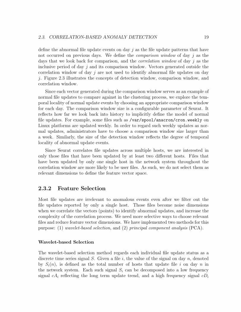
define the abnormal file update events on day j as the file update patterns that havenot occurred on previous days. We define the comparison window of day j as thedays that we look back for comparison, and the correlation window of day j as theinclusive period of day j and its comparison window. Vectors generated outside thecorrelation window of day j are not used to identify abnormal file updates on dayj. Figure 2.3 illustrates the concepts of detection window, comparison window, andcorrelation window.
Since each vector generated during the comparison window serves as an example ofnormal file updates to compare against in the clustering process, we explore the tem-poral locality of normal update events by choosing an appropriate comparison windowfor each day. The comparison window size is a configurable parameter of Seurat. Itreflects how far we look back into history to implicitly define the model of normalfile updates. For example, some files such as /var/spool/anacron/cron.weekly onLinux platforms are updated weekly. In order to regard such weekly updates as nor-mal updates, administrators have to choose a comparison window size larger thana week. Similarly, the size of the detection window reflects the degree of temporallocality of abnormal update events.
Since Seurat correlates file updates across multiple hosts, we are interested inonly those files that have been updated by at least two different hosts. Files thathave been updated by only one single host in the network system throughout thecorrelation window are more likely to be user files. As such, we do not select them asrelevant dimensions to define the feature vector space.
2.3.2 Feature Selection
Most file updates are irrelevant to anomalous events even after we filter out thefile updates reported by only a single host. Those files become noise dimensionswhen we correlate the vectors (points) to identify abnormal updates, and increase thecomplexity of the correlation process. We need more selective ways to choose relevantfiles and reduce feature vector dimensions. We have implemented two methods for thispurpose: (1) wavelet-based selection, and (2) principal component analysis (PCA).
Wavelet-based Selection
The wavelet-based selection method regards each individual file update status as adiscrete time series signal S. Given a file i, the value of the signal on day n, denotedby Si(n), is defined as the total number of hosts that update file i on day n inthe network system. Each such signal Si can be decomposed into a low frequencysignal cAi reflecting the long term update trend, and a high frequency signal cDi

20CHAPTER 2. ANOMALY DETECTION USING SPATIOTEMPORAL EVENT CORRELATION
Number of host
day
Daily variations
Long term update trend
Figure 2.4: Representing file update status with wavelet transformation. The originalsignal is S, which can be decomposed into a low frequency signal cA reflecting thelong term update trend, and a high frequency signal cD reflecting the daily variationsfrom the long-term trend.
reflecting the day-to-day variation from the long term trend (see Figure 2.4). If thehigh frequency signal cDi shows a spike or a dip on a certain day, we know that asignificantly larger or smaller number of hosts updated file i than on a normal day,respectively. We then select file i as a relevant feature dimension in defining thefeature vector space.
Seurat detects signal spikes and dips using the residual signal of the long-termtrend. The similar technique has been used to detect disease outbreaks [119] andnetwork traffic anomalies [7]. To detect anomalies on day j, the algorithm takes asinput the list of files that have been updated by at least two different hosts in thecorrelation window of day j. Then, from these files the algorithm selects a subsetthat will be used to define the feature vector space.
Figure 2.5 shows the steps to select features by wavelet-based method. Givena fixed correlation window of day j, the algorithm starts with constructing a timeseries signal Si for each file i, and decomposes Si into cAi and cDi using a single-level Daubechies wavelet transformation as described. Then we compute the residualsignal value Ri(j) of day j by subtracting the trend value cAi(j−1) of day j−1 fromthe original signal value Si(j) of day j. If |Ri(j)| exceeds a preset threshold α, thenthe actual number of hosts who have updated file i on day j is significantly largeror smaller than the prediction cAi(j − 1) based on the long term trend. Therefore,Seurat selects file i as an interesting feature dimension for anomaly detection on dayj. As an example, Figure 2.6 shows the original signal and the residual signal of a fileusing a 32-day correlation window in a 22-host teaching cluster. Note the threshold

2.3. CORRELATION-BASED ANOMALY DETECTION 21
For each file i:
1. Construct a time series signal:Si = cAi + cDi
2. Compute the residual signal value of day j:Ri(j) = Si(j) − cAi(j − 1)
3. if |Ri(j)| > α, then select file i as a feature dimension.
Figure 2.5: Wavelet-based feature selection.
0 10 20 30 40 50 600
2
4
6
8
10
12
14
16
18
20
Days
Num
ber
of h
osts
0 10 20 30 40 50 60−20
−15
−10
−5
0
5
10
15
Days
Res
idua
l Sig
nal,
Ri
(a) (b)
Figure 2.6: Wavelet transformation of file update status. (a) The original signal ofthe file update status (b) The residual signal after wavelet transformation
value α of each file is a parameter selected based on the statistical distribution ofhistorical residual values.
PCA-based Dimension Reduction
PCA is a statistical method to reduce data dimensionality without much loss ofinformation [43]. Given a set of d-dimensional data points, PCA finds a set of d′-dimensional vectors, called principal components, that account for the variance of theinput data as much as possible. Dimensionality reduction is achieved by projectingthe original d-dimensional data onto the subspace spanned by these d′ orthogonalvectors. Most of the intrinsic information of the d-dimensional data is preserved inthe subspace.

22CHAPTER 2. ANOMALY DETECTION USING SPATIOTEMPORAL EVENT CORRELATION
We note that the updates of different files are usually correlated. For example,when a software package is updated on a host, many of the related files will be modifiedtogether. Thus we can perform PCA to identify the correlation of file updates.
Given a d-dimensional feature space Zd2 , and a list of m feature vectors V1,V2, . . .,
Vm ∈ Zd2 , we perform the following steps using PCA to obtain a new list of feature
vectors V ′1,V
′2, . . . ,V
′m ∈ Zd′
2 (d′ < d) with reduced number of dimensions:
1. Standardize each feature vector Vk = 〈v1k, v2k, . . . , vdk〉 (1 ≤ k ≤ m) by sub-tracting each of its elements vik by the mean value of the corresponding di-mension ui(1 ≤ i ≤ d). We use V k = 〈v1k, v2k, . . . , vdk〉 ∈ Zd
2 to denote thestandardized vector for the original feature vector Vk. Then,
vik = vik − ui (where ui =
∑m
j=1 vij
m, 1 ≤ i ≤ d)
2. Use the standardized feature vectors V 1 ,V 2 , . . . ,V m as input data to PCAin order to identify a set of principal components that are orthogonal vectorsdefining a set of transformed dimensions of the original feature space Zd
2 . Se-lect the first d′ principal components that account for most of the input datavariances (e.g., 90% of data variances) to define a subspace Zd′
2 .
3. Project each standardized feature vector V k ∈ Zd2 onto the PCA selected sub-
space Zd′
2 to obtain the corresponding reduced dimension vector V ′k∈ Zd′
2 .
Note that PCA is complementary to wavelet-based selection. Once we fix thecorrelation window of a particular day, we first pick a set of files to define the featurevector space by wavelet-based selection. We then perform PCA to reduce the datadimensionality further.
2.3.3 Anomaly Detection by Clustering
Once we obtain a list of transformed feature vectors using feature selection, we clusterthe vectors based on the distance between every pair of them.
We call the cluster a new cluster if it consists of multiple vectors only from thedetection window. The appearance of a new cluster indicates a change in file updatepatterns occurred during the detection window and should raise an alarm.
There are many existing algorithms for clustering, for example, K-means [33, 34] orSingle Linkage Hierarchical Clustering [45]. Seurat uses a simple iterative algorithm,which is a common method for K-means initialization, to cluster vectors without priorknowledge of the number of clusters [62]. The algorithm assumes each cluster has a

2.4. EXPERIMENTS 23
hub. A vector belongs to the cluster whose hub is closest to that vector comparedwith the distances from other hubs to that vector. The algorithm starts with onecluster whose hub is randomly chosen. Then, it iteratively selects a vector that hasthe largest distance to its own hub as a new hub, and re-clusters all the vectorsbased on their distances to all the selected hubs. This process continues until thereis no vector whose distance to its hub is larger than the half of the average hub-hubdistance.
We choose this simple iterative algorithm because it runs much faster, and worksequally well as the Single Linkage Hierarchical algorithm in our experiments. Thereason that even the simple clustering algorithm works well is that the ratio of inter-cluster distance to intra-cluster distance significantly increases after feature selection.
Once we detect a new cluster and generate an alarm, we can further identify theinvolved hosts and the files from which the cluster resulted. The suspicious hosts arejust the ones whose file updates correspond to the feature vectors in the new cluster.To determine which files possibly cause the alarm, we only focus on the files pickedby the wavelet-based selection to define the feature vector space. For each of thosefiles, if it is updated by all the hosts in the new cluster during the detection window,but has not been updated by any host during the corresponding comparison window,Seurat outputs this file as a candidate file. Similarly, Seurat also reports the set offiles that have been updated during the comparison window, but are not updated byany host in the new cluster during the detection window.
Based on the suspicious hosts and the selected files for explaining root causes,system administrators can decide whether the updates are known administrative up-dates that should be suppressed, or some abnormal events that should be furtherinvestigated. If the updates are caused by malicious attacks, administrators can takeremedial counter measures for the new cluster. Furthermore, additional compromisedhosts can be identified by checking if the new cluster expands later and if other hostshave updated the same set of candidate files. Note that the alarms due to adminis-trative updates can be suppressed if the administrator provides Seurat with the listof involved files beforehand.
2.4 Experiments
We have developed a multi-platform (Linux and Windows) prototype of Seurat thatconsists of a lightweight data collection tool and a correlation module. The datacollection tool scans the file system of the host where it is running and generates adaily summary of file update attributes. Seurat harvests the summary reports frommultiple hosts in a network system and the correlation module uses the reports foranomaly detection.
24CHAPTER 2. ANOMALY DETECTION USING SPATIOTEMPORAL EVENT CORRELATION
We have installed the Seurat data collection tool on a number of campus officemachines and a teaching cluster that are used by students daily. By default, the toolscans the attributes of all system files on a host. The attributes of a file include the filename, type, device number, permissions, size, inode number, important timestamps,and a 16-byte MD5 checksum of file content. Each day, each host compares thenewly scanned disk snapshot against that from the previous day and generates a fileupdate summary report. In the current prototype, all the reports are uploaded dailyto a centralized server where system administrators can monitor and correlate the fileupdates using the correlation module.
In this section, we study the effectiveness of Seurat’s pointillist approach for de-tecting aggregated anomalous events. Using the daily file update reports from ourreal deployment, we study the false positive rate and the corresponding causes inSection 2.4.1 and Section 2.4.2. We evaluate the false negative rate with simulatedattacks in Section 2.4.3. In order to verify the effectiveness of our approach on realmalicious attacks, we launched real worms and viruses into isolated computer clusters.We report the results in Section 2.4.4 and Section 2.4.5.
2.4.1 False Positives on Linux Platforms
The best way to study the effectiveness of our approach is to test it with real data. Wehave deployed the Seurat data collection tool on both Linux and Windows hosts, andcorrelate the reports for daily anomaly detection. The results from both deploymentsare similar. We first illustrate the details of the experiment and the results with thedata from our Linux host deployment, where we have longer period of data collectionthan for our Windows deployment. Then, we describe the results of the Windowshost deployment briefly in Section 2.4.2.
We deployed Seurat on a teaching cluster of 22 Linux hosts and have been collect-ing the daily file update reports since Nov 2003. The teaching cluster is mostly usedby students for their programming assignments. The cluster is also occasionally usedby a few graduate students for running network experiments. For privacy protection,personal files under user home directories are not scanned for Linux platforms.
In this experiment, we use the file update reports from Dec 1, 2003 until Feb 29,2004 to evaluate the false positive rate. During this period, there are a few dayswhen a couple of hosts failed to generate or upload reports due to system failure orreconfigurations. For those small number of missing reports, we simply ignore thembecause they do not affect the aggregated file update patterns.
We set the correlation window to 32 days in order to accommodate monthly fileupdate patterns. That is, we correlate the update pattern from day 1 to day 32 toidentify abnormal events on day 32, and correlate the update pattern from day 2 to

2.4. EXPERIMENTS 25
day 33 to detect anomalies on day 33, etc. Thus, our detection starts from Jan 1,2004, since we do not have 32-day correlation windows for the days in Dec 2003.
Dimension Reduction
Once we fixed the correlation window of a particular day, we identify relevant filesusing wavelet-based selection with a constant threshold α = 2 to define the featurevector space for simplicity. We then perform PCA to reduce the data dimensionalityfurther by picking the first several principal components that account for 98% of theinput data variance.
Throughout the entire period of 91 days, 772 files with unique file names wereupdated by at least two different hosts. Figure 2.7 (a) shows the number of hoststhat updated each file during the data collection period. We observe that only asmall number files (e.g.,/var/adm/syslog/mail.log) are updated regularly by all ofthe hosts, while most other files (e.g., /var/run/named.pid) are updated irregularly,depending on the system usage or the applications running.
Figure 2.7 (b) shows the results of feature selection. There were, on average, over2000 files updated by hosts in the cluster during each correlation window (i.e., oneday). Among those files, there were on average 140 files updated by at least twodifferent hosts daily. After wavelet-based selection, the average number of featuredimensions is 17. PCA further reduces the vector space dimension to an average of2. Overall, we achieved about 3 orders of magnitude dimensionality reduction.
Days since Dec 1, 2003
File
ID (
sort
ed)
10 20 30 40 50 60 70 80 90
100
200
300
400
500
600
700
10 20 30 40 50 6010
0
101
102
103
Days since Jan 1, 2004
Num
ber
of D
imen
sion
s
Total files updatedFiles updated by multiple hostsDimensions after waveletDimensions after PCA
(a) (b)
Figure 2.7: Feature selection and dimension reduction. (a) File update patterns. Filesare sorted by the cumulative number of hosts that have updated them throughoutthe 91 days. The darker the color is, the more hosts updated the corresponding file.(b) The number of feature vector dimensions after wavelet-based selection and PCAconsecutively.

26CHAPTER 2. ANOMALY DETECTION USING SPATIOTEMPORAL EVENT CORRELATION
False Alarms
173
26
322
36
20
1
84
17 15
4
10
01−19−04
66
16
13
6595
27
89
49
49
2757 53
81
11
14
01−20−04
261
909
165
58
8035
7
01−21−04
New Cluster!
436
21
241
3
01−22−04
165
3436
2
159 22
6
01−23−04
New Cluster! 151
16222
72
19694
6
01−24−04
Figure 2.8: Clustering feature vectors for anomaly detection at Linux platforms. Eachcircle represents a cluster. The number at the center of the figure shows the totalnumber of clusters. The radius of a circle corresponds to the number of points in thecluster, which is also indicated beside the circle. The squared dots correspond to thenew points generated on the day under detection. New clusters are identified by athicker circle.
After dimension reduction, we perform clustering of feature vectors and identifynew clusters for each day. Figure 2.8 illustrates the clustering results of 6 consecutivedays from Jan 19, 2004 to Jan 24, 2004. There are two new clusters identified on Jan21 and Jan 23, which involve 9 hosts and 6 hosts, respectively. Since Seurat outputsa list of suspicious files as the cause of each alarm, system administrators can tell ifthe new clusters are caused by malicious intrusions.
Based on the list of files output by Seurat, we can figure out that the new clusterson Jan 21 and Jan 23 reflect large scale file updates due to a system reconfigurationat the beginning of the spring semester. For both days, Seurat accurately pinpointsthe exact hosts that are involved. The reconfiguration started from Jan 21, when alarge number of binaries, header files, and library files were modified on 9 out of the22 hosts. Since the events are known to system administrators, we treat the identifiedvectors as normal for future anomaly detection. Thus, no alarm is triggered on Jan22, when the same set of library files were modified on 12 other hosts. On Jan 23,the reconfiguration continued to remove a set of printer files on 6 out of the 22 hosts.

2.4. EXPERIMENTS 27
Again, administrators can mark this event as normal and we spot no new cluster onJan 24, when 14 other hosts underwent the same set of file updates.
In total, Seurat raises alarms on 9 out of the 60 days under detection, amongwhich 6 were due to system reconfigurations. Since the system administrators areaware of such events in advance, they can simply suppress these alarms. The 3 otheralarms are generated on 3 consecutive days when a graduate student performed anetwork experiment that involved simultaneous file updates at multiple hosts. Suchevents are rare, and should alert the system administrators.
2.4.2 False Positives on Microsoft Windows Platforms
We installed the Seurat data collection tool on 15 Microsoft Windows XP machinesthat are office desktops used by volunteering faculty and graduate students in a cam-pus network. We have collected file update reports daily from these machines sinceSeptember 2004.
Since there are no default user home directories for Windows platforms, all the filesin the C:\ drive are scanned, including the C:\Documents and Settings\ directorywhere user related Windows registry files (which are more likely to be modified by anattack) reside. Note each Windows user will have a common set of similar directoriesand files under the directory C:\Documents and Settings\userid\ where “userid”is the user’s Windows login ID. In such cases, we convert the “userid” in the pathname to a generic user ID in order to both correlate the changes of user-relatedWindows registry files and preserve user privacy. Consequently, we may have moreunique files updated across multiple machines to perform Seurat correlation than thecase where we only look at system file changes.
For this experiment, we use the file update reports from Sep 10, 2004 until Oct25,2004, when the majority of the volunteered machines are running the Seurat datacollection tool. Similar to the data collected from our Linux deployment, there are afew days in this period when a couple of hosts failed to upload reports because theirusers turned off the machines or temporarily disabled the Seurat data collection toolfor running their own timing-critical tasks.
We again set the correlation window size to 32 days. As such, our anomalydetection starts from Oct 11, 2004 and lasts for 15 days.
Dimension Reduction
Throughout the entire period of 46 days, 18,072 files with unique file names (afterconverting user IDs to a generic user ID) were updated by at least two different hostson Windows platforms. We pick the 500 most frequently updated files out of the total

28CHAPTER 2. ANOMALY DETECTION USING SPATIOTEMPORAL EVENT CORRELATION
Days since Sep 11, 2004
File
ID (
sort
ed)
5 10 15 20 25 30 35 40
50
100
150
200
250
300
350
400
450
5002 4 6 8 10 12
100
101
102
103
104
105
Days since Oct 12, 2004
Num
ber
of D
imen
sion
s
Total files updatedFiles updated by multiple hostsDimensions after waveletDimensions after PCA
(a) (b)
Figure 2.9: Feature selection and dimension reduction at Microsoft Windows Plat-forms. (a) File update patterns. Files are sorted by the cumulative number of hoststhat have updated them throughout the 46 days. The darker the color is, the morehosts updated the corresponding file. (b) The number of feature vector dimensionsafter wavelet-based selection and PCA consecutively.
18,072 files, and Figure 2.9 (a) shows the number of hosts that updated each suchselected file during the data collection period. Compared with the data from our Linuxdeployment, the Windows file update patterns are less regular. One reason is that themonitored machines are under different administrative subdomains, unlike the Linuxteaching cluster where the machines have more homogeneous configurations. Thus,the locations of non-standardized applications in the file system could be differentacross different machines. We found that only a small number of log files are updatedregularly by most of the hosts (e.g., C:\WINDOWS\security\logs\winlogon.log).However, the majority of file update patterns are irregular, depending on the actuallylaunched applications and how the system is being used.
Figure 2.9 (b) shows the Seurat feature selection results on the Windows machinesduring the 15 days of anomaly detection. Although we observe significantly more dailyfile updates on participating Windows hosts than Linux hosts, the average number offiles that are updated by at least two different hosts during each correlation window is165, similar to the Linux hosts. Wavelet-based selection reduces the average numberof feature dimensions to 22, and PCA further reduces the number of dimensions toan average of 10 every day.
False Alarms
Seurat raised one alarm during the 15 days of anomaly detection from Oct 11, 2004to Oct 25, 2004. The alarm was raised on Oct 18, 2004, when two new clusters were

2.4. EXPERIMENTS 29
identified with each cluster involving two participating hosts. The lists of suspiciousfile changes reported by Seurat suggest that both new clusters were caused by Win-dows Update2. In one new cluster, the set of files identified are all located underthe directory C:\Program Files\WindowsUpdate. For the other new cluster, Seuratoutput 30 files which had not been updated by any host before but were updatedby the two corresponding hosts in the new cluster. Most of these identified files aredll library files under the directory C:\WINDOWS\system32, suggesting that the filemodification events might be related to system updates. After talking to the ownersof the two involved hosts, we confirmed that the detected machines indeed installed aWindows update package called “Cumulative Security Update for Internet Explorerfor Windows XP Service Pack 2 (KB834707)” on the same day that Seurat spottedthe new cluster.
2.4.3 False Negatives
The primary goal of this experiment is to study the false negative rate and detectionlatency of Seurat as the stealthiness of the attack changes. We use simulated attacksby manually updating files on the selected host reports, as if they were infected.
We first examine the detection rate of Seurat by varying the degree of attack ag-gressiveness. We model the attack propagation speed as the number of hosts infectedon each day (the detection window), and model the attack stealthiness on a localhost as the number of new files installed by this attack. Our simulation runs on thesame teaching cluster that we described in Section 2.4.1. Since the aggregated fileupdate patterns are different for each day, we randomly pick ten days in Feb 2004,when there was no intrusion. On each selected day, we simulate attacks by manuallyinserting artificial new files into a number of host reports on only that day, and usethe modified reports as input for detection algorithm. We then remove those modifiedentries, and repeat the experiments with another day. The detection rate is calculatedas the number of days that Seurat spots new clusters over the total ten days.
Figure 2.10 shows the detection rate of Seurat by varying the number of filesinserted on each host and the number of hosts infected. On one hand, the detectionrate monotonically increases as we increase the number of files inserted on each hostby an attack. Since the inserted files do not exist before, each of them will be selectedas a feature dimension by the wavelet-based selection, leading to larger distancesbetween the points of infected host state changes and the points of normal host statechanges. Therefore, the more new files are injected by an attack, the higher thedetection rate gets. On the other hand, as we increase the number of infected hosts,
2More information on Windows Update can be found at http://windowsupdate.microsoft.comand http://go.microsoft.com/fwlink?linkid=23699
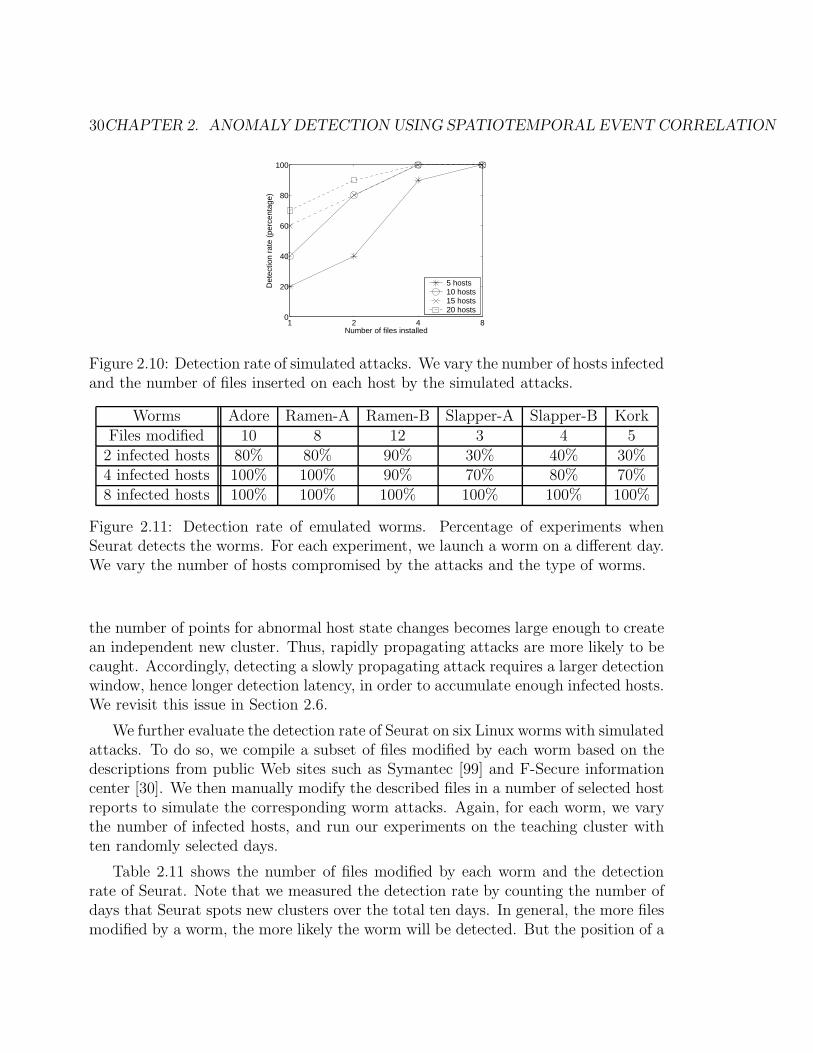
30CHAPTER 2. ANOMALY DETECTION USING SPATIOTEMPORAL EVENT CORRELATION
1 2 4 80
20
40
60
80
100
Number of files installed
Det
ectio
n ra
te (
perc
enta
ge)
5 hosts10 hosts15 hosts20 hosts
Figure 2.10: Detection rate of simulated attacks. We vary the number of hosts infectedand the number of files inserted on each host by the simulated attacks.
Worms Adore Ramen-A Ramen-B Slapper-A Slapper-B KorkFiles modified 10 8 12 3 4 5
2 infected hosts 80% 80% 90% 30% 40% 30%4 infected hosts 100% 100% 90% 70% 80% 70%8 infected hosts 100% 100% 100% 100% 100% 100%
Figure 2.11: Detection rate of emulated worms. Percentage of experiments whenSeurat detects the worms. For each experiment, we launch a worm on a different day.We vary the number of hosts compromised by the attacks and the type of worms.
the number of points for abnormal host state changes becomes large enough to createan independent new cluster. Thus, rapidly propagating attacks are more likely to becaught. Accordingly, detecting a slowly propagating attack requires a larger detectionwindow, hence longer detection latency, in order to accumulate enough infected hosts.We revisit this issue in Section 2.6.
We further evaluate the detection rate of Seurat on six Linux worms with simulatedattacks. To do so, we compile a subset of files modified by each worm based on thedescriptions from public Web sites such as Symantec [99] and F-Secure informationcenter [30]. We then manually modify the described files in a number of selected hostreports to simulate the corresponding worm attacks. Again, for each worm, we varythe number of infected hosts, and run our experiments on the teaching cluster withten randomly selected days.
Table 2.11 shows the number of files modified by each worm and the detectionrate of Seurat. Note that we measured the detection rate by counting the number ofdays that Seurat spots new clusters over the total ten days. In general, the more filesmodified by a worm, the more likely the worm will be detected. But the position of a

2.4. EXPERIMENTS 31
file in the file system directory tree also matters. For example, both Slapper-B wormand Kork worm insert 4 new files into a compromised host. However, Kork wormadditionally modifies /etc/passwd to create accounts with root privileges. Becausethere are many hosts that have updated /etc/passwd during a series of system re-configuration events, the inclusion of such files in the feature vector space reduces thedistances from abnormal points to normal points, resulting in higher false negativerates. We discuss this further in Section 2.6.
2.4.4 Real Attacks on Linux Platforms
Now we proceed to examine the efficacy of Seurat during a real worm outbreak. Thebest way to show this would be to have Seurat detect an anomaly caused by a newworm propagation. Instead of waiting for a new worm’s outbreak, we have set up anisolated computer cluster where, without damaging the real network, we can launchworms and record file system changes. This way, we have full control over the numberof hosts infected, and can repeat the experiments. Because the isolated cluster hasno real users, we merge the data acquired from the isolated cluster with the data wehave collected from the Linux teaching cluster in order to conduct experiments.
We obtained the binaries and source codes of a few popular worms from publicWeb sites such as whitehats [111] and packetstorm [72]. Extensively testing Seurat,with various real worms in the isolated cluster, requires tremendous effort in settingup each host with the right versions of vulnerable software. As such, we limit ourattention to one worm for illustrative purposes and present the result with the Lionworm [86] in this experiment.
The Lion worm was found in early 2001. Lion exploits a vulnerability of BIND8.2, 8.2-P1, 8.2.1, 8.2.2-Px. Once Lion infects a system, it sets up backdoors, leaksout confidential information (/etc/passwd, /etc/shadow) via email, and scans theInternet to recruit vulnerable systems. Lion scans the network by randomly pick-ing the first 16 bits of an IP address, and then sequentially probing all the 216 IPaddresses in the space of the block. After that, Lion randomly selects another suchaddress block to continue scanning. As a result, once a host is infected by Lion, allthe vulnerable hosts nearby (in the same IP address block) will be infected soon.Lion affects file systems: the worm puts related binaries and shell scripts under the/dev/.lib directory, copies itself into the /tmp directory, changes system files underthe /etc directory, and tries to wipe out some log files.
We configured the isolated cluster with three Lion-vulnerable hosts and one addi-tional machine that launched the worm. The vulnerable machines were running Red-Hat 6.2 including the vulnerable BIND 8.2.2-P5. The cluster used one C class networkaddress block. Every machine in the cluster was connected to a 100Mbps Ethernet

32CHAPTER 2. ANOMALY DETECTION USING SPATIOTEMPORAL EVENT CORRELATION
and was running a DNS server (named) of the BIND distribution as a caching-onlyname server. This setup is similar to the Linux teaching cluster described in Sec-tion 2.4.1, where all the hosts are running named as caching-only servers for efficientdomain name lookup. The Seurat data collection tool generated a file system updatereport on every machine daily.
177
481
40
3
02−10−04
171
37
211311
38
38
47
255
97
16
12
02−11−04
New Cluster!
338
75
201
85
4
02−12−04
Figure 2.12: Intrusion detection by Seurat. Seurat identified a new cluster of threehosts on Feb 11, 2004, when we manually launched the Lion worm. The number ofclusters formed in each day varies due to an artifact of the feature vector selectionand the clustering algorithm.
After we launched the Lion worm, all three vulnerable hosts in the isolated clusterwere infected quickly one after another. We merge the file update report by the eachcompromised host with a different normal host report generated on Feb 11, 2004,when we know there was no anomaly. Figure 2.12 shows the clustering results ofthree consecutive days from Feb 10, 2004 to Feb 12, 2004 using the merged reports.
On the attack day, there are 64 files picked by the wavelet-based selection. Thenumber of feature dimensions is reduced to 9 after PCA. Seurat successfully detectsa new cluster consisting of the 3 infected hosts. Figure 2.13 lists the 22 files selectedby Seurat as the causes of the alarm. These files provide enough hints to the adminis-trators to confirm the existence of the Lion worm. Once detected, these compromisedhosts as well as the list of suspicious files can be marked for future detection. If, inthe following days, there are more hosts that are clustered together with the alreadyinfected machines, or experience the same file updates, then we may conclude theyare infected by the same attack.
2.4.5 Real Attacks on Microsoft Windows Platforms
In recent years, the number of worms and viruses targeting Windows platforms hasincreased dramatically. The Symantec company reported 4,496 new instances of ma-licious code exploiting vulnerabilities of the Microsoft Windows systems during the

2.4. EXPERIMENTS 33
File ID. File name File ID. File name1 /sbin/asp 12 /var/spool/mail
2 /dev/.lib 13 /dev/.lib/bindx.sh
3 /dev/.lib/star.sh 14 /tmp/ramen.tgz
4 /var/spool/mail/root 15 /dev/.lib/scan.sh
5 /dev/.lib/bind 16 /dev/.lib/pscan
6 /etc/hosts.deny 17 /var/spool/mqueue
7 /dev/.lib/randb 18 /dev/.lib/hack.sh
8 /sbin 19 /dev/.lib/.hack
9 /var/log 20 /dev/.lib/index.html
10 /dev/.lib/bindname.log 21 /dev/.lib/asp62
11 /dev/.lib/index.htm 22 /var/log/sendmail.st
Figure 2.13: Suspicious files for the new cluster on Feb 11, 2004.
first six months of 2004 only [100]. In this section, we examine the effectiveness ofSeurat in detecting worm/virus infections on Windows systems.
We obtained the executables of recently found Windows worms and viruses, man-ually launched them in an isolated computer cluster of 6 vulnerable, unpatched Win-dows XP hosts inside one C class network address space. The 6 Windows XP hostsare virtual machines deployed over 3 physical machines connected to a 100Mbps Eth-ernet running VMWare. For the scanning worms (i.e., Blaster worm), we launchedthem from a seed machine and let them propagate. For viruses that need humanusers to activate them, we emulated the virus propagations by manually clicking thevirus-infected programs or documents at each host (i.e., mass-mailing viruses such asLoveLetter, NetSky, Bagle). The Seurat data collection tool then reported the filesystem updates on every Windows virtual machine daily. We merged the reportedfile changes with the reports from our real Windows system deployment described inSection 2.4.2.
In order to examine the performance with different attack propagation rates, weagain vary the number of hosts infected each time and randomly select 10 days toinject attacks. Figure 2.14 lists the detection rates of the Windows worms and virusesthat we manually launched inside the cluster and the number of suspicious files iden-tified to explain the corresponding root causes.
For every attack, Seurat detected the appearance of a new cluster with high prob-ability and successfully pinpointed the exact compromised hosts that were involvedeven when there were only 2 hosts infected. In the Blaster worm case, after we injectedthe attack into the isolated cluster, only 4 out of the 6 Windows virtual machinesactually got infected. The other two were not infected for undetermined reasons.
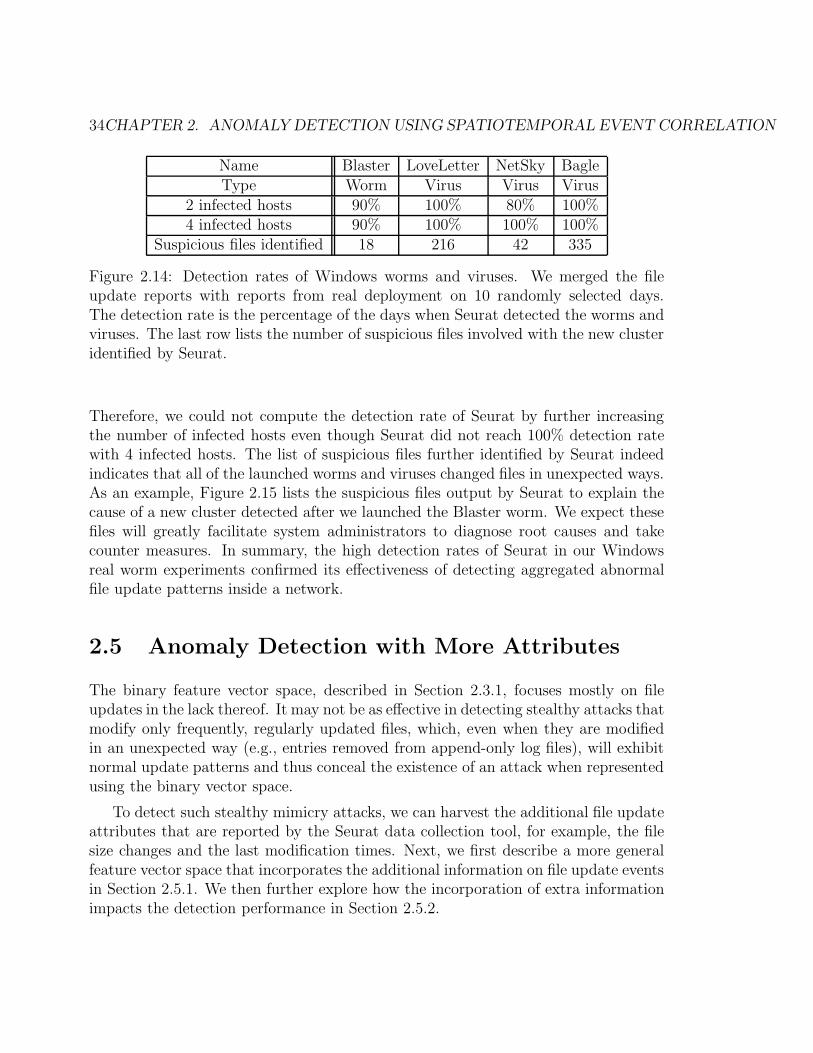
34CHAPTER 2. ANOMALY DETECTION USING SPATIOTEMPORAL EVENT CORRELATION
Name Blaster LoveLetter NetSky BagleType Worm Virus Virus Virus
2 infected hosts 90% 100% 80% 100%4 infected hosts 90% 100% 100% 100%
Suspicious files identified 18 216 42 335
Figure 2.14: Detection rates of Windows worms and viruses. We merged the fileupdate reports with reports from real deployment on 10 randomly selected days.The detection rate is the percentage of the days when Seurat detected the worms andviruses. The last row lists the number of suspicious files involved with the new clusteridentified by Seurat.
Therefore, we could not compute the detection rate of Seurat by further increasingthe number of infected hosts even though Seurat did not reach 100% detection ratewith 4 infected hosts. The list of suspicious files further identified by Seurat indeedindicates that all of the launched worms and viruses changed files in unexpected ways.As an example, Figure 2.15 lists the suspicious files output by Seurat to explain thecause of a new cluster detected after we launched the Blaster worm. We expect thesefiles will greatly facilitate system administrators to diagnose root causes and takecounter measures. In summary, the high detection rates of Seurat in our Windowsreal worm experiments confirmed its effectiveness of detecting aggregated abnormalfile update patterns inside a network.
2.5 Anomaly Detection with More Attributes
The binary feature vector space, described in Section 2.3.1, focuses mostly on fileupdates in the lack thereof. It may not be as effective in detecting stealthy attacks thatmodify only frequently, regularly updated files, which, even when they are modifiedin an unexpected way (e.g., entries removed from append-only log files), will exhibitnormal update patterns and thus conceal the existence of an attack when representedusing the binary vector space.
To detect such stealthy mimicry attacks, we can harvest the additional file updateattributes that are reported by the Seurat data collection tool, for example, the filesize changes and the last modification times. Next, we first describe a more generalfeature vector space that incorporates the additional information on file update eventsin Section 2.5.1. We then further explore how the incorporation of extra informationimpacts the detection performance in Section 2.5.2.

2.5. ANOMALY DETECTION WITH MORE ATTRIBUTES 35
File ID. File name1 C:\WINDOWS\system32\msblast.exe2 C:\WINDOWS\Prefetch\MSBLAST.EXE-09FF84F2.pf3 C:\WINDOWS\bootstat.dat4 C:\WINDOWS\system32\config\SECURITY5 C:\WINDOWS\Prefetch\TFTP.EXE-2FB50BCA.pf6 C:\WINDOWS\system32\wpa.dbl7 C:\WINDOWS\0.log8 C:\WINDOWS\system329 C:\WINDOWS\system32\config\SAM10 C:\WINDOWS\system32\config\default11 C:\Program Files\VMware\VMware Tools\tools.conf12 C:\WINDOWS\Prefetch\NETSTAT.EXE-2B2B4428.pf13 C:\WINDOWS\Debug\oakley.log14 C:\WINDOWS\system32\config\systemprofile\Cookies\index.dat15 C:\Documents and Settings\gluser\Local Settings\desktop.ini16 C:\WINDOWS\Debug\oakley.log.sav17 C:\WINDOWS\system32\wbem\Logs18 C:\WINDOWS\system32\config\default.LOG
Figure 2.15: Suspicious files identified to explain the cause of a new cluster detectedafter we launched the Blaster worm.
2.5.1 A General Feature Vector Space
This section describes a general feature vector space that incorporates the additionalfile update information. Similar to the binary vector space, each dimension in thegeneral vector space corresponds to a unique file. The value of each dimension,however, will be a numerical value reflecting the degree of change of the correspondingattribute of interest (e.g., file size change). The distance D(V1,V2) between a pair offeature vectors V1 and V2 is defined as their Euclidean distance:
D(V1,V2) = ||V1 − V2||2
In the above formula, ||.||2 denotes the L2 norm. With such representation, twovectors with a small Euclidean distance are more likely to have similar values alongevery dimension and thus experience similar updates. In our current prototype, weconsider only homogeneous file attributes when defining the general feature vectorspace. That is, we do not consider different types of attributes (e.g., file size and lastmodification time) simultaneously in the same vector space.

36CHAPTER 2. ANOMALY DETECTION USING SPATIOTEMPORAL EVENT CORRELATION
Given a file update attribute, we can use different ways to set the numerical valueof a dimension. We consider file size changes and last modification times in ourcurrent prototype as they can be naturally represented as numerical values in thefollowing ways:
• File size change: We expect that for each file associated with a propagatingattack, the number of bytes changed across different compromised hosts wouldbe close to each other. So given a file, we define the value of the correspondingdimension to be the number of bytes increased in a detection window (i.e., oneday). A negative value indicates file size decrease, while a zero value suggestsno file size change.
• Last modification time: The temporal locality of file updates due to attackssuggests that abnormal updates usually occur close in time with each other.Thus, for each file, we define the value of the corresponding dimension to bethe last modification time in terms of the number of minutes elapsed sincethe beginning of a detection window (12:00 pm for each day in our currentprototype).
We note that the Euclidean distance computation weighs each dimension equally.Thus the distance between two vectors could be dominated by a small number ofdimensions with larger differences. For example, a file whose size increased from 1,000bytes to 2,000 bytes will have more impact on the computed distance than another filewhose size increased from 1000 bytes to 1020 bytes. We take the 3-month file updatereports collected from our Linux system deployment and examine the distributions ofthe one dimensional difference in feature vector spaces defined by file size changes andlast modification times in Figure 2.16 (a) and (b), respectively. For each dimension(i.e., each file), we compute the average difference between every possible pair ofvectors that Seurat generated during the entire data collection period. We observethat the one dimensional difference is highly biased across different dimensions (up to7 orders of magnitude different) for both file size changes and last modification times.Such highly skewed distribution suggests that we need to normalize the values acrossdifferent feature dimensions when computing the Euclidean distances.
In our current prototype, Seurat uses a standard max-min normalization method [45].We normalize all the values of a dimension to within the range [−100, 100]. That is,for the i-th dimension, the maximal positive value vmax+
i is normalized to 100, whilethe minimal negative value vmin−
i is normalized to −100. Any other value vi of thesame dimension will be normalized to vnorm
i , where
vnormi =
{100 × (vi/v
max+i ) if vi ≥ 0
−100 × (vi/vmin−i ) if vi < 0

2.5. ANOMALY DETECTION WITH MORE ATTRIBUTES 37
0 200 400 600 80010
−4
10−2
100
102
104
106
File ID (sorted)
Ave
rage
diff
eren
ce (
byte
s)
0 100 200 300 400 500 600 700 80010
−2
10−1
100
101
102
103
File ID (sorted)
Ave
rage
diff
eren
ce (
min
utes
)
(a) (b)
Figure 2.16: The distribution of average one-dimensional difference across all dimen-sions (each dimension corresponds to a unique file). (a) Average difference betweenfile size changes. (b) Average difference between last modification times.
Note there is a special case at data normalization when a file is deleted duringa detection window. Seurat currently sets the value of a dimension to the minimalnegative normalized value (i.e., −100) if the corresponding file is removed. This isconsistent with the current definition of the feature dimension values. In the caseof file size changes, a file removal event would result in the maximal decrease ofthe number of bytes, hence minimal negative value change. In the case of file lastmodification time, there will be no exact timestamp of when a file is removed usingthe current 1 day file update scanning cycle. Hence we use the minimal negative valueto represent the unknown removal time. An alternative way is to treat file removalsas special events that will be represented (and hence detected) only using the binaryfeature vectors.
2.5.2 Performance Impact
In this section, we examine how the incorporation of additional file update attributeswill impact the detection rate and the false positive rate. We again use file sizechanges and last modification times to define the general feature vector space foranomaly detection. We use two sets of data for this experiment: (1) the file updatereports collected from our real Linux deployment, and (2) the file update reports fromthe isolated cluster where we manually launched the Linux Lion worm.
Similar to the experiments with binary feature vectors, we set the correlationwindow size to 32 days, and use wavelet-based analysis to select a subset of relevantfiles. We then normalize the values of the selected feature dimensions and perform

38CHAPTER 2. ANOMALY DETECTION USING SPATIOTEMPORAL EVENT CORRELATION
Reasons for Alarms Number of AlarmsDetected using System reconfiguration events 6
binary vector space Network-wide experiment 3Not detected using Unseen file updates detected 3binary vector space Unseen update patterns detected 10
Figure 2.17: False alarms generated using feature vectors defined by file size changes.
PCA to further reduce the data dimensionality.
Attribute I: File Size Changes
We first use only file size changes to define the general feature vector space. Through-out the 60 days of detection under real deployment, Seurat, with this general featurevector space, raised a total of 22 alarms.
In order to understand why Seurat generated more alarms than by using the binaryvector space, we examine the cause of each alarm based on the list of the suspiciousfiles identified after clustering, and categorize the alarms in Figure 2.17.
We observe that using the general feature vector space, Seurat not only identifiedall the abnormal file update events that are detected by using the binary vectors,but also detected 10 file size update patterns that have not been observed before.Further inspection based on the abnormal file size update patterns suggests they aremostly caused by the log file size changes due to the variations of system usage daily.We expect that the number of such false alarms will be reduced by setting a largercorrelation window to accommodate more instances of regular updates. Seurat alsoidentified three events when each time there is a single new file being modified for thefirst time across 3, 6, and 5 hosts, respectively. We list the date and the file nameidentified for each of these 3 events in Figure 2.18. Again, we could investigate thembased on the identified files. We found that, after each event, all the other hosts in theLinux cluster had the same file updates on the following day, which results in all hostsin the cluster being updated at last. They were administrative update that could befiltered if administrators provided Seurat with the update schedule beforehand. Sincethese three events changed only a single new file each time, they are more likely toevade detection using only the binary feature vector space with a low detect rate aswe have explained in Section 2.4.3.
We proceed to examine the efficacy of the general feature vector space using themanually launched Linux Lion worm. Again, we merged the file update reports fromthe compromised hosts with the reports collected from the Linux teaching cluster onFeb 11, 2004. Seurat successfully identified a new cluster of the exact three compro-

2.5. ANOMALY DETECTION WITH MORE ATTRIBUTES 39
Date in 2004 Number of hosts File nameJan 28 3 /var/spool/lpd/norton
Feb 6 6 /etc/printcap
Feb 23 5 /usr/local/lib/nannyconfig/qpage
Figure 2.18: Details of the three events when a single new file was modified for thefirst time. ”Number of hosts” means the number of hosts involved in each file updateevent.
mised hosts using the file size change information. Figure 2.19 shows the clusteringresults on the day we injected the attack.
689
1
3
2
1
1
2
7
02−11−04
New Cluster
Figure 2.19: Seurat identifies a new cluster of the exact three infected hosts by theLion worm with the general feature vector space defined using file size changes.
The above experiment results suggest that both the detection rate and the falsepositive rate will be more sensitive to the general vector space defined by file sizechanges compared with the binary vector space. On one hand, Seurat will be ableto detect stealthy attacks that result in unexpected file size changes or install a verysmall number of new files with the additional information, and hence increase thedetection rate. On the other hand, the false positive rate will also rise as legitimateunseen file size change patterns may also be misclassified as intrusion attempts. Thereis thus a tradeoff of detection rate and false positive rate when using the differenttypes of feature vector spaces.
Attribute II: Last Modification Time
In this section, we use the last modification times to define the general feature vectorspace and repeat our experiments. Seurat also generated a total of 22 alarms dur-

40CHAPTER 2. ANOMALY DETECTION USING SPATIOTEMPORAL EVENT CORRELATION
Reasons of Alarms Number of AlarmsDetected using System reconfiguration events 6
binary vector space Network-wide experiment 3Not detected using Unseen file updates detected 1binary vector space Unseen update patterns detected 12
Figure 2.20: False alarms generated using feature vectors defined by last modificationtimes.
ing the 60 days of anomaly detection using the file update reports from our Linuxdeployment (see Figure 2.20).
Similar to using file size changes, Seurat successfully identified all of the 9 alarmsthat were previously detected by using the binary feature vectors. A closer lookat these 9 alarms, which were caused by system reconfigurations and network wideexperiments, showed that they indeed have strong temporal correlations of file updatesacross different hosts. For majority of the rest of the alarms, however, Seurat couldnot pinpoint a small number files to explain for the new cluster. They are causedby the unseen overall update time patterns, suggesting that there exists no strongregularity of the last modification times across different hosts.
When we further evaluate Seurat with the manually launched Lion worm, it failedto detect the attack by generating a new cluster. Instead, using the general featurevector space defined by last modification times, each of the 3 vectors correspondingto the 3 compromised hosts forms an independent cluster itself. More careful inves-tigation reveals that, although the Lion worm injected new files into a compromisedhost and caused unexpected file update time patterns on the same day, the infectiontimes of the 3 compromised hosts are not close enough to be clustered together dueto the attack propagation delay. This is because our data normalization described inSection 2.5.1 amplifies the differences between file update times. One way to addressthe problem is to use coarser granularity timestamps, for example, hours instead ofminutes. However, selecting a best time granularity requires prior knowledge of at-tack propagation speed. In addition, attackers can more easily exploit the coarsergranularity timestamps to blend the abnormal file updates with normal file updates.We plan to further investigate a more robust way of feature representation using lastmodification times as future work to this thesis.

2.6. DISCUSSION 41
2.6 Discussion
By identifying parallel occurrences of coincident events, Seurat will be most successfulin detecting attacks that result in file modifications at multiple hosts. Certain attacks(e.g., password guessing attacks) that succeed only once or a few times in a networksystem may evade Seurat detection. The current prototype of Seurat also has limiteddetection capability to the following types of attacks.
Stealthy attack. Attackers may try to evade detection by slowing attack propaga-tion. If an attacker is patient enough to infect only one host a day in the monitorednetwork system, Seurat will not notice the intrusion with the current one-day detec-tion window because Seurat focuses only on anomalous file changes common acrossmultiple hosts. A larger detection window such as a couple of days or a week can helpto catch slow, stealthy attacks. Note, however, that Seurat notices the attacks onlyafter multiple hosts in the network system are compromised. In other words, if anattack propagates slowly, Seurat may not recognize the attack for the first few daysafter the initial successful compromise. There is thus a tradeoff between detectionrate and detection latency.
Mimicry attack. An attacker can carefully design his attack to cause file updatesthat look similar to regular file changes, and mount a successful mimicry attack [104]by cloaking abnormal file updates with many normal but irregular changes duringSeurat’s clustering process. For example, in Section 2.4.3, we observed that the falsenegative rate of detecting the Kork worm was relatively higher due to the interferenceof irregular system reconfiguration. We leave it as future work to quantify this typeof mimicry attack and the effectiveness of possible counter measures.
Random-file-access attack. Seurat correlates file updates based on their completepath names. Thus attackers can try to evade Seurat by installing attack files underdifferent directories at different hosts, or replacing randomly chosen existing files withattack files. Many recent email viruses already change the virus file names when theypropagate to a new host; we envision similar techniques could be employed by othertypes of attacks soon. Note, however, that even the random-file-access attack mayneed a few anchor files at fixed places, where Seurat still has the opportunity to detectsuch attacks. A more robust representation of a file, for example, an MD5 checksum,could help Seurat detect random-file-access attacks.
Memory-resident attack. Memory-resident and BIOS-resident only attacks makeno file system updates. Thus Seurat will not be able to detect memory residentattacks by examining host file updates, nor those attacks that erase disk evidencebefore the Seurat data collection tool performs the scheduled disk scan.
Kernel/Seurat modification attack. The effectiveness of Seurat relies on the cor-rectness of reports from the data collecting tools running on distributed hosts. So the

42CHAPTER 2. ANOMALY DETECTION USING SPATIOTEMPORAL EVENT CORRELATION
host kernels and the Seurat data collection tools should run on machines protectedby trusted computing platforms [102]. An alternative solution is to monitor file sys-tem changes in real time (will be discussed further in Section 2.7) and to protect fileupdate logs using secure audit logging (e.g., [89]).
2.7 Future Work
Real-time anomaly detection. The current prototype periodically scans and reportsfile system updates with a 1-day cycle, which may be slow to detect fast propagatingattacks. To shorten detection latency, we are enhancing the Seurat data collectionmodule to monitor system calls related with file updates, and report the changesimmediately to the correlation module. The reported file updates will be instantlyreflected by setting the corresponding bits in the feature vectors at the Seurat corre-lation module, which continuously performs clustering of the new feature vectors forreal time anomaly detection.
Distributed correlation module. Currently, Seurat moves the daily reports fromdistributed data collection tools to a centralized server, where the correlation mod-ule computes and clusters the host vectors. Despite the simplicity of centralizeddeployment, the centralized approach exposes Seurat to problems in scalability andreliability. First, since the input to the correlation are low level file update events,the amount of report data to be transferred to and stored at the centralized server islarge. In our experience, a host generates a file update report of 3K-140KBytes dailyin a compressed format, so the aggregate report size from hundreds or thousandsof hosts with a long comparison window will be large. The report size will be largerwhen Seurat’s data collection tool reports the host state changes in real time. Second,the monitored hosts could be in different administrative domains (i.e., hosts managedby different academic departments or labs) and it is often impractical to transferthe detailed reports from all the hosts to one centralized server due to privacy andconfidentiality issues. Third, the centralized server can be a single point-of-failure.It is important for Seurat to work even when one correlation server is broken or apart of network is partitioned. A distributed correlation module will cope with thoseissues. As future work, we can investigate methods to correlate file update events ina distributed architecture such as EMERALD [79], AAFID [6], and Mingle [115].
Other applications. The approach of clustering coincident host state changes canbe generalized to other types of applications such as detecting the propagation of spy-ware, illegal file sharing events, or erroneous software configuration changes. We arecurrently deploying Seurat on Planetlab [1] hosts for detecting software configurationerrors by identifying host state vectors that do not fall into an expected cluster.

Chapter 3
Network Forensics Using
Spatiotemporal Event Correlation
3.1 Introduction
Many types of Internet attacks utilize indirection as a means to hide their source. Forexample, the act of utilizing a chain of compromised machines, or “stepping stones,”in an attack is a common means of foiling a defender’s attempts to locate the source ofan attack. Similarly, distributed denial-of-service (DDoS) attacks are often launchedfrom compromised computers, sometimes called “zombies”, both to harness the powerof many machines and to obfuscate where the true source of the attack lies.
In all these attacks that utilize compromised computers to launch attack traffic, theoverwhelming majority of the attack traffic originates from victims of the attack, asopposed to the true source of the attack. Such indirection is a highly successful meansto provide anonymity to attackers, and to date there is little automated support foridentifying the location (computer or network) from which such an attack is launched.Similarly, when an intranet succumbs to such an attack, there is little automated helpto determine the internal computer that was compromised first.
In this thesis, we define an approach with the promise to dramatically changeinvestigations of Internet-based attacks. Our high-level vision is an investigativecapability for the Internet or intranets that permits identification and fine-grainedanalysis of the communication patterns leading to an attack, particularly includingthose attacks that utilize indirection as a means to hide their true source. Our goalis to bridge indirection techniques, such as stepping stones and zombies, to locate theoriginal source of the attack or entry point to an intranet and to reconstruct how anattack unfolded.
43

44CHAPTER 3. NETWORK FORENSICS USING SPATIOTEMPORAL EVENT CORRELATION
We believe that this capability can significantly strengthen the hand of adminis-trators in deterring attacks or permitting the correction of weak points in a networkperimeter. For example, if an attack that propagated within an intranet can be tracedback to its initial entry into the intranet—e.g., revealing an errant service or modempermitting connections that circumvent the firewall, or a user who is careless in theemail attachments he opens—then that entry point can be corrected. And, of course,the ability to trace large-scale attacks to their ultimate source is a first step towardholding that attacker accountable.
While attacks can propagate via various rates and methods, use different sig-natures, and exploit different vulnerabilities, there is an invariant across all types(present and future) of attacks: for an attack to progress, there must be communica-tion among attacker and the associated set of compromised hosts. Attacks utilizingindirection often exhibit network behavior that may not seem suspicious at the levelof individual flows, but will nevertheless exhibit a discernible pattern when traffic isobserved collectively. Such observation can be exploited to detect and trace attacks.
In this thesis, we formalize the problem of network forensic analysis, and presenta Dragnet framework to define the required infrastructure and its properties wheresuch observation can be exploited. In particular, we focus on the specific problemof crafting an algorithm that determines the origin of epidemic spreading attackssuch as Internet worms. Our goal is not only to identify the “patient zero” of theepidemic, but also to reconstruct the sequence of attack flows that make up theinitial stages of the attack tree via which the worm infected successive generationsof victims. Instead of studying specific attacks that have been seen in the wild, wepresent an algorithm called random moonwalks that works by identifying the overallstructure of an attack’s propagation using spatiotemporal event correlation. Sincethe algorithm assumes no prior knowledge about attack specific properties, it can beagnostic to attack signatures or scanning rates, and potentially be applicable to allworm attacks.
The random moonwalk algorithm in essence is a Monte Carlo sampling methodthat identifies the “wide tree” structure of a worm propagation by performing randomwalks backward in time along paths of network flows. Correlating the flows traversedby repeated walks reveals the initial attack path, thereby aiding in identifying thesource. Such algorithm is inherently robust to small amounts of missing data, and canbe elegantly adapted to distributed scenarios where multiple domains collaborativelyperform forensic analysis without sharing private data. We demonstrate throughanalysis, simulation, and experiments on real world traces that this approach can behighly effective in locating the origin of a wide class of worm attacks that propagatevia different strategies, without the use of attack signatures.
The rest of this chapter is organized as follows. We first formalize the problemof network forensics in Section 3.2. We then outline an architecture for providing

3.2. PROBLEM FORMULATION 45
such new capability in Section 3.3. Section 3.4 describes the proposed algorithm foridentifying the worm origins and the initial causal flows. We analytically study theeffectiveness of the algorithm in Section 3.6. Section 3.7 and Section 3.8 evaluatethe method using real-world network traces and simulation traces, respectively. Sec-tion 3.9 presents a formal interpretation of our algorithm, where we show that thealgorithm can be regarded as performing spectral analysis on a flow graph constructedfrom the network trace. In Section 3.10, we discuss distributed forensic analysis inpractice, examine the impact of missing data on performance, and present a dis-tributed random moonwalk algorithm to allow multiple administrative domains foridentifying the worm origin collaboratively. In Section 3.11, we study variations ofour algorithm, where we may incorporate additional knowledge with biased samplingstrategies. Finally, we discuss in Section 3.12 deployment issues as well as futurework.
3.2 Problem Formulation
We define the problem of tracing and reconstruction of arbitrary network attacksin terms of two fundamental components, Attacker Identification and Attack Recon-struction. These act as building blocks on which attack investigation can be basedand attackers held accountable. Attacker Identification is the ability to accuratelypinpoint the source(s) of the attack or infection. Attack Reconstruction is the processof inferring which communications carry the attack forward. This not only identifiesthe compromised hosts for subsequent correction, but also provides crucial informa-tion about the attack propagation that can help in precluding future attacks of asimilar kind. The focus of our work on identifying the true source of attacks throughAttacker Identification and Attack Reconstruction differentiates it from other effortsthat seek to identify when an attack is occurring or to reactively blunt the effect ofan attack already in progress.
Figure 3.2 shows a general model of how an arbitrary network attack propagatesfrom one host to another across administrative domains. We mark each of the attackflows with a timestamp to indicate when the attack was received by the victim. Theattack originates at host A at time t1, and then propagates to hosts B to H.
We model these network communication events between end-hosts using a directedhost contact graph G = 〈V, E〉. The nodes of the graph V = H × T , where H is theset of all hosts in the network and T is time. Each directed edge represents a networkflow between two end hosts at a certain time, where the flow has a finite duration,and involves transfer of one or more packets. We represent each edge by a tuplee = 〈u, v, ts, te〉 where u ∈ H is the host that initiates the communication (the sourceof the flow), v ∈ H is the host that receives the communication (the destination of
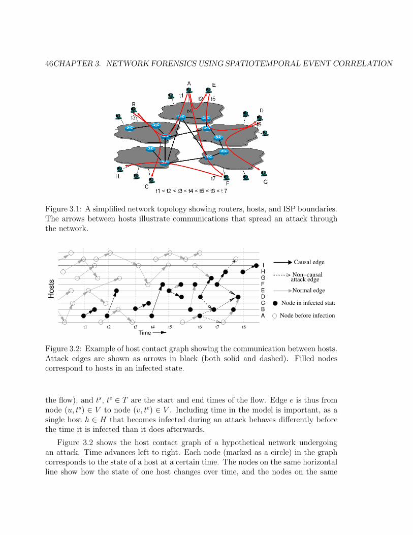
46CHAPTER 3. NETWORK FORENSICS USING SPATIOTEMPORAL EVENT CORRELATION
Figure 3.1: A simplified network topology showing routers, hosts, and ISP boundaries.The arrows between hosts illustrate communications that spread an attack throughthe network.
Node before infection
Node in infected state
Normal edge
Causal edge
attack edgeNon−causal
t3 t4 t5 t6 t7
Hosts
H
G
F
E
D
C
B
A
Time
t1 t2 t8
I
Figure 3.2: Example of host contact graph showing the communication between hosts.Attack edges are shown as arrows in black (both solid and dashed). Filled nodescorrespond to hosts in an infected state.
the flow), and ts, te ∈ T are the start and end times of the flow. Edge e is thus fromnode (u, ts) ∈ V to node (v, te) ∈ V . Including time in the model is important, as asingle host h ∈ H that becomes infected during an attack behaves differently beforethe time it is infected than it does afterwards.
Figure 3.2 shows the host contact graph of a hypothetical network undergoingan attack. Time advances left to right. Each node (marked as a circle) in the graphcorresponds to the state of a host at a certain time. The nodes on the same horizontalline show how the state of one host changes over time, and the nodes on the same

3.2. PROBLEM FORMULATION 47
A
Bt1
Et2
F
t4
Ct3
Dt5
Ht7
Gt6
It8
Figure 3.3: Example showing the causal tree, which contain causal edges with times-tamps from the host contact graph.
vertical line represent the states of different hosts at the same time.
Each directed edge in Figure 3.2 represents a network flow. If a flow does notcarry an infectious payload, we call that edge a normal edge. We define an edge as anattack edge (highlighted in the figure as either dashed or solid arrows) if it correspondsto a flow that carries attack traffic, whether or not the flow is successful in infectingthe destination host. While a worm attack may induce a large number of attack flowsin the network, only a few flows actually advance the attack by successfully infectinga new host. We define an edge as a causal edge (highlighted as a solid arrow) if itcorresponds to a flow that actually infects its destination. For example, at time t6,host D has attack edges to both hosts G and B. However, only the edge from D to Gis a causal edge because G is infected by this contact, whereas B was infected earlierbefore time t2.
The causal tree formalizes the concept of epidemic attack spread. The causal treeis formed by extracting the causal edges from the host contact graph and projectingthe edges along the time axis. To be consistent with the notion of time in the hostcontact graph, we consider causal edges occurring earlier in time as edges in the higherlevels of the causal tree. Figure 3.2 shows the causal tree for the attack in Figure 3.2,with each edge annotated with a timestamp. The edge with timestamp t1 from theworm origin A is thus at the highest level of the tree.
Given the host contact graph, Attack Reconstruction identifies which edges arecausal edges that advanced the attack. Even infected hosts may continue their nor-mal activities and not all infection attempts succeed, so Attack Reconstruction mustcarefully infer which communication initiated by an infected host should be markedas carrying the attack, and reconstruct the host attack tree using the marked edges.Attacker Identification operates by working its way back up the causal tree to findthe root sources of the attack. Even when the ultimate root and source of the attacktree cannot be found (e.g., due to missing data), the higher level nodes of the causaltree that are reconstructed point the way toward the true attack source and providea starting point for out-of-band human investigation.

48CHAPTER 3. NETWORK FORENSICS USING SPATIOTEMPORAL EVENT CORRELATION
3.3 A Framework For Investigating Attacks
Identifying the propagation of an attack is particularly difficult as the adversary isintelligent: attackers are bound to come up with smarter mechanisms trying to evadedetection. However, there is one fundamental invariant across all attacks (presentand future): for the attack to progress there must be communication among attacker,the associated set of compromised hosts and the victim(s), and this communicationis visible to the network.
The communication between attackers and victims may be subtle and invisiblewhen observed from any single host without foreknowledge of the attack signature,but it will potentially stand out when viewed globally as the attack propagates. Asa simple example, efforts to detect stepping stones have been premised on the iden-tification of flows that exhibit closely correlated packet contents or inter-packet tim-ings [120, 28]; while each flow in isolation may seem innocuous, together they revealsuspicious behavior. In general, our approach is to develop algorithms that correlatethe communication events among individual hosts across both space and time, andidentify the patterns that indicate a propagating attack. Since no accurate signa-ture is required, our approach has the potential to be robust against changes in thebehavior of attacks.
Applying our approach to a large scale network requires a means to: (1) gatherand query host communication records from distributed network locations; and (2)design analysis algorithms for identifying global communication patterns given thehost contact graph.
3.3.1 Network Auditing
We need widely deployed infrastructure support where distributed collection pointslog traffic records and store them in repositories for querying. As has been discussed inSection 3.2, we focus on end-host connectivity patterns in terms of directional network“flows”, where each flow identifies a directional communication event between a sourceand a destination, and carries timestamps indicating the start and stop time of theflow. Compared with packet traces, flow records are more compact representationsand need not capture packet payloads, which might be construed as a violation ofend-user privacy.
At the scale of an intranet, traffic logging can be deployed as pervasively as neces-sary. At the Internet scale, the problem of obtaining an approximation of the completehost contact graph appears intractable. However, there are features of the Internettopology and routing that suggest auditing devices can be deployed at a relativelysmall number of locations to approximately construct the host contact graph. First,

3.3. A FRAMEWORK FOR INVESTIGATING ATTACKS 49
0.1
0.2
0.3
0.4
0.5
0.6
0.7
0.8
0.9
1
0 10 20 30 40 50 60 70 80 90 100
Fra
ctio
n of
pat
hs c
over
ed
Number of top k ases cooperating
Coverage of AS Paths
Figure 3.4: Path coverage vs number of highest degree ASes selected.
Internet routing is highly constrained by inter-domain policies and the AS hierarchy,which implies that top level ASes will observe a significant fraction of the traffic.Second, the Internet AS-level connectivity graph has been shown to be a power-lawgraph [31], suggesting that high degree ASes are good candidates for logging deploy-ment.
To estimate how many observation points should be deployed in the Internet fora given fraction of the flows to be logged at least once, we investigate the optimalpath coverage problem, related to the problem of deploying reverse path filters [74]and containment filters [64], assuming flows uniformly distribute among all availableInternet paths. We define an AS graph G = 〈V, E〉, where V is the set of ASes, andE is the set of inter-AS connections. Let P be the set of paths used for routing trafficin G. We say an AS a (a ∈ V ) covers a path p (p ∈ P ) if a is on the path p. Giventhese notions, we want to select the smallest AS subset V ′ ⊆ V that covers α percentof the paths in P .
We consider a greedy heuristic where the ASes are selected based on their degrees,with higher degree ASes given higher preference. Figure 3.4 shows the fraction of AS-paths that are “covered” by the first k high-degree ASes, using AS paths and ASdegrees obtained from RouteViews [84] in Feb 2004. The figure shows that if the 50ASes with highest node degrees deployed flow auditing, these ASes would “cover”approximately 90% of all the paths, and hence be able to log any flow traversing oneof these paths.
To help reveal the causal relationship between flows for attack reconstruction,ideally all logging devices in the auditing infrastructure should have perfect timesynchronization (perhaps achieved using GPS time sources or NTP [71]. In reality,the logging points will be located in diverse geographical locations and across multipleASes, and time synchronization cannot be guaranteed. However, it appears bothpractical and sufficient to ensure two flows are timestamped consistent with the causalrelationship between them (if any) [55]. “Causal consistent timestamps” mean thatif a flow A is, in fact, caused by flow B, then A will have a timestamp later than

50CHAPTER 3. NETWORK FORENSICS USING SPATIOTEMPORAL EVENT CORRELATION
A
B
CE
F
G
D
Figure 3.5: Concept behind attack reconstruction: the probability of being involvedin an attack should be reinforced by network events. The fraction of host filled inrepresents the probability that host is involved in an attack, as computed by anintrusion detection system. Given the probability of B and E’s involvement and thecommunication pattern between the hosts, the likelihood of C, D, and F’s involvementshould be increased.
B. This property is achieved if there is any single router that records both flows ofinterest or if there are any two time-synchronized routers (e.g., they are in the sameadministrative domain) where flow A is recorded by one router and flow B by theother.
3.3.2 Techniques for Attack Reconstruction
The key component of the analysis lies in the algorithmic components that analyze thedata log to extract “interesting” communication patterns that are part of an ongoingnetwork attack. The attack reconstruction algorithms may operate over a centralizeddata repository (in the case of an intranet), or will need to interact with distributedquery routing and data retrieval mechanisms (in the case of a larger internet). Thereexists an entire spectrum of design decisions that may involve fundamental tradeoffsregarding issues such as scalability, effectiveness of the solutions, susceptibility toevasion, and overall performance. These design decisions will also have to take intoconsideration the deployment scenario, as the requirements and capabilities for anInternet vs Intranet scale analysis framework are vastly different.
One general category of reconstruction methods is to reveal the causal relation-ship between communications by spatially correlating local observations. Figure 3.5illustrates the concept. The fraction of each host that is filled in represents the prob-ability that that host is involved in the attack. These initial probability estimatesare based on locally observed behavior, such as those a local host-based IntrusionDetection System (IDS) might observe. Based on the local observations alone, it is

3.3. A FRAMEWORK FOR INVESTIGATING ATTACKS 51
likely B and E are involved in an attack. Given the communication pattern amongthe hosts, however, it is extremely likely that hosts C, D, and F are also involved,although their locally observable behavior was not suspicious enough to trigger anIDS.
Initial Local Observations
The input to Attack Reconstruction is one or more estimates of the probability thata host is involved in an attack. We can leverage prior work in this area, as theseestimates can come from any existing IDS or network monitoring system that detectsthe occurrence of attacks in the network. For example, we can use measures suchas the fanout of the host in any given time interval, the rate at which the hostgenerates traffic, and the set of destinations that the host contacted within a timeinterval. For each of these measures, we can use anomaly detection mechanisms toobserve deviations from normal behavior and compute a confidence estimate for theprobability an host is involved in an attack.
Attack Reconstruction Using Host Contact Graphs
Given the initial probabilities of hosts involved in an attack, the host contact graphobtained from the audit logs can be used to refine the involvement probability es-timates and reconstruct the attack. The goals are to: (1) identify the edges thatsuccessfully attack a new host (i.e., are causal) and (2) the top-level nodes of thecausal tree.
In this thesis, we explore one particular algorithm using random moonwalks toidentify the origin of epidemic spreading attacks such as Internet Worms by findinginitial causal flows on the causal tree. The algorithm takes network flows betweenend hosts as initial local observations, and assumes uniformly distributed probabilityestimate of a host being compromised. Given a host contact graph, the goal of ouralgorithm is to identify a set of edges that, with high probability, are edges from thetop level(s) (i.e., initial in time) of the causal tree. Among the hosts listed as thesources of these edges will be the origin of the attack (or the host at which the attackfirst entered the intranet). It is critical that the technique have a reasonably low false-negative rate, so that the returned set contains at least one top level causal edge thatidentifies the attack origin. It is desirable that the technique have a low false-positiverate, so that the returned set does not include many normal edges, attack edges thatdo not infect the destination, or even causal edges that occur lower in the causal tree,since the sources of these edges are less likely to be the true origin of the attack.
In the next several sections, we focus on this specific algorithm, where we applythe spatiotemporal event correlation approach. We start by exploring the algorithm

52CHAPTER 3. NETWORK FORENSICS USING SPATIOTEMPORAL EVENT CORRELATION
in a centralized scenario where we have the complete host contact graph available. Wethen theoretically study the algorithm to understand how it analyzes the underlyinggraph structure. Finally, we look at algorithm extensions in a distributed environmentwhere portions of data might be missing, and each party can share only limitedinformation.
3.4 The Random Moonwalk Algorithm
Given the complete knowledge of a host contact graph, our algorithm consists ofrepeatedly sampling paths from the graph and then correlating these samples. Theedges that occur most frequently among the samples are selected as the edges mostlikely to be causal edges from levels higher up in the causal tree. The first key tothe technique is that we do not sample individual edges — rather, each sample is acontiguous path of edges in the graph. The second key is that we create the pathby starting at a randomly chosen edge, and then walking backwards in time alongthe graph, randomly choosing among potential predecessor edges at each step in themoonwalk.
The sampling process is controlled by three parameters: W - the number of walks(i.e., samples) performed, d - the maximum length of the path traversed by a singlewalk, and ∆t - the sampling window size defined as the maximum time allowedbetween two consecutive edges in a walk. Each walk starts at an arbitrarily chosenedge e1 = 〈u1, v1, t
s1, t
e1〉 representing a flow from host u1 to host v1. We then pick a
next step backward in time uniformly from the set of edges that arrived at u1 withinthe previous ∆t seconds. That is, an edge e2 = 〈u2, v2, t
s2, t
e2〉 such that v2 = u1 and
te2 < ts1 < te2 + ∆t. Each walk stops when there is no edge within ∆t seconds tocontinue the path, or the path has traversed the specified maximum number of hopsd.
As the sampling is performed, a count is kept of how many times each edgefrom the host contact graph is traversed. After W walks have been performed, thealgorithm returns the Z edges with the highest counts. Here, Z is a user specifiedparameter to determine how many edges are to be returned for further investigation.These edges are most likely to be top-level causal edges from the causal tree. Asdefined and used in this paper, the algorithm operates off-line with the parametersand host contact graph as inputs. As future work, we are investigating on-line versionsthat may also dynamically tune parameters.
Each random moonwalk made by the algorithm samples a potential causal chainof events. Because the walks wander into the past, the edge at step i (time = t1)in a walk could be potentially caused by the edge at step i + 1 (time = t2, wheret2 < t1). Since the walks begin at different randomly chosen edges, an edge that

3.5. EVALUATION METHODOLOGY 53
shows up frequently among many walks has the potential to be indirectly responsiblefor causing a large number edges in the host contact graph. Worm attacks have theproperty that a small number of edges (those high up in the causal tree) are indirectlyresponsible for causing a large number of edges in the host contact graph (the attackedges lower in the tree). Thus the edges implicated by our sampling algorithm arelikely to be those high in the causal tree.
Two factors appear to aid in the convergence of the sampling algorithm, althoughit remains future work to determine the relative importance of each factor.
First, an infected host generally originates more flows than it receives. If the wormmakes attack attempts very rarely this difference may be slight, but sending attackflows increases the rate of outgoing flows without increasing the rate of incomingflows. The result is that there are more edges that can lead a walk to an infected hostthan there are edges that lead away from it. This tends to concentrate walks towardsthe root of the tree.
Second, in normal communication patterns today, most hosts are clients thatinitiate communication with servers, and so are the originators of flows in the hostcontact graph. Since hosts receive relatively few flows, random moonwalks in a hostcontact graph without an ongoing worm attack tend to be very short, as many edgeshave no predecessors within the ∆t sampling window. Worms, port scanning, andpeer-to-peer systems are among the few applications that cause hosts to receive flows,and port scanning or peer-to-peer systems tend to lack the tree-structure that causerandom moonwalks to concentrate.
3.5 Evaluation Methodology
We evaluate the random moonwalk algorithm using an analytical study, real trace ex-periments, and simulations, with different models of background traffic and differentworm propagation rates. We first present in Section 3.6 analytical results with a sim-plified traffic model, showing that the random moonwalk technique has promise, andgive analytical estimates on the performance of the algorithm. Section 3.7 presentsexperimental results with a large real network trace, to demonstrate the success of thealgorithm in discovering the initial causal edges under various attack scenarios includ-ing worms propagating at very slow rates. We also discuss how to select parametervalues for maximum walk length d and sampling window ∆t for an arbitrary networktrace. For completeness, we present in Section 3.8 a set of simulation experiments toshow the performance of the algorithm under different background traffic models.
As discussed earlier, the output of the random moonwalk algorithm is a set of theZ edges that were traversed most frequently during the W moonwalks. Given the

54CHAPTER 3. NETWORK FORENSICS USING SPATIOTEMPORAL EVENT CORRELATION
Z returned edges, we use three performance metrics to evaluate the performance ofthe algorithm: (1) the detection accuracy in terms of the number of causal edges andattack edges returned, (2) the false positive rate of the set of edges returned, and (3)the number of suspect hosts identified by the algorithm as potential origins of theworm.
As our goal is to identify the initial causal edges whose source is the worm origin,attack edges and even causal edges from lower levels of the causal tree are consideredas false positives. In the analytical study, we develop a model for reasoning aboutthe false positive rates associated with finding only the top-level causal edges. In realattacks, the notion of top-level edges loses meaning, since the assumptions simplifyingthe notion of time and the unit duration of a flow (made in the analysis) no longerhold. Therefore, in the simulation and real trace studies, we evaluate performanceusing detection accuracy of the number of causal edges among the Z top frequencyedges. We then use experiments to show that the majority of the returned causaledges are from the highest levels of the causal tree, with the worm origin as one ofthe sources of the edges.
3.6 Analytical Model
In this section, we present an analytical model that explains how well the randommoonwalk sampling process works and why. Using the analytical model, we showhow we can predict the sampling performance achieved from W walks with maximumlength d and given ∆t.
3.6.1 Assumptions
To enable tractable analysis of the random moonwalk sampling, we make simplifyingassumptions about the structure of the host contact graph and the attack. Althoughour model is an over-simplification of real network traffic, it enables an estimationpredicting the performance of the technique and sheds light on the intuition behindthe effectiveness of the technique.
First, we assume the host contact graph is known, and it contains |E| edges and|H| hosts.
Second, we discretize time into units. We assume every flow has a length of oneunit, and each flow starts at the beginning of a unit and finishes before the start ofthe next unit.
Third, we define the start time of the first attack flow, T0, to be the origin ofthe time axis. Combined with the second assumption, this means that rather than

3.6. ANALYTICAL MODEL 55
T0 + k T0 + (k-1) T0 + (k+1)
e = <u,v,k>
v
u
Figure 3.6: An edge at time k in the host contact graph.
describing both the start and end times of an edge in terms of continuous time vari-ables, we can refer to its “time” as k = te − T0 using just the flow end time te. Thefirst attack edge is then at time k = 1, and an edge e = 〈u, v, ts, te〉 is at time k ifte = T0 + k (illustrated in Figure 3.6). In the analysis below, we use ek to denotean edge at time k, ek = 〈u, v, k〉. Edges that occurred before T0 will have negative kvalues.
Fourth, we assume a normal host initiates B concurrent outgoing flows at eachtime unit. Once a host is infected, it starts malicious scanning by initiating a totalof A outgoing flows at each subsequent time unit. The A outgoing flows includeB normal flows and A − B attack flows. Both the normal hosts and the infectedhosts randomly select a destination host for every flow. Unlike a normal flow, notevery attack flow will go to a valid host address. Suppose only fraction r of theaddress space is being used, then among the A−B concurrent outgoing attack flows,R = (A−B)× r will go to existing hosts, while the rest A−B −R will go to invaliddestinations. This results in an infected host initiating a total of B +R flows to validdestinations each time unit. The rate at which the worm spreads is thus determinedby both A, the rate of scanning, and R, the effectiveness of the scans.
Finally, we assume that flows and packets are not lost or blocked, so that flowssent to a valid host are received by that host. This means that the total number offlows sent to valid hosts at time k − 1 will be the total number of flows received attime k. If the fraction of infected hosts at time k − 1 is given by f(k − 1), then eachhost at time k will receive an average of I(k) flows, where
I(k) = (B + R) × f(k − 1)︸ ︷︷ ︸
+ B × (1 − f(k − 1))︸ ︷︷ ︸
(3.1)
Flows from infected hosts Flows from normal hosts

56CHAPTER 3. NETWORK FORENSICS USING SPATIOTEMPORAL EVENT CORRELATION
With the notions introduced above, we can simplify the random moonwalk algo-rithm described in Section 2.3. For each walk, once we select an edge e1 = 〈u1, v1, k1〉as our current step, we consider an edge e2 = 〈u2, v2, k2〉 as a candidate next steponly if v2 = u1 and k2 + 1 = k1, i.e., ∆t = 1.
3.6.2 Edge Probability Distribution
With the above assumptions and notation, we show analytically that the initial causalflows are more likely to be traversed by a random moonwalk, and thus be selected foridentifying the ultimate source or entry point of the attack. We do so by estimatingP (e) — the probability of an edge e being traversed in a random moonwalk on thehost contact graph.
We classify edges into two categories based on their destinations. We define anedge ek
m = 〈u, v, k〉 as a malicious-destination edge if v is infected before or at timek. Otherwise, we define the edge as a normal-destination edge denoted as ek
n. Sincea causal edge will successfully infect the destination host immediately, a causal edgeis always a malicious-destination edge. With the two categories of edges, we have thefollowing approximations:
P (ekw) ≈
1|E|
[
1 + AI(k)
+(B+R)×
P
d−2
i=1Tk+i
I(k)I(k+1)
]
w = m;
1|E|
[
1 + BI(k)
+B×
P
d−2
i=1Tk+i
I(k)I(k+1)
]
w = n.
where Tk = Af(k) + B[1 − f(k)].
We present how we derive the above estimates in the Appendices (Chapter 6.1).Based on the above observations, the probability difference between the two categoriesof edges is estimated as:
P (ekm) − P (ek
n) ≈1
|E|
[
A − B
I(k)+
R∑d−2
i=1 Tk+i
I(k)I(k + 1)
]
(3.2)
For fast propagating worms, A >> B and R > 0, so it is clear malicious-destination edges (hence causal edges) have higher probability of being selected bythe random moonwalks than normal-destination edges. The difference between thetwo probabilities (hence the effectiveness of random moonwalks) increases as the pathlength d increases and as the scanning rate A increases (i.e., the worm is more ag-gressive).
The analytic model presented in this section makes a worst-case assumption that

3.6. ANALYTICAL MODEL 57
Number of Edges |E| 4.9 × 10⁷
Number of Hosts |H| 105
Vulnerable fraction F 0.1Valid host space r 0.5Normal rate B 2Infection rate A 400Attack start time 0Attack stop time 15
Figure 3.7: The parameters of a host contact graph with a fast propagating worm.
both normal and attack traffic choose the destination for each flow uniformly fromamong all possible hosts. Therefore, it cannot predict the performance of the algo-rithm on worms that send attack flows less frequently than normal flows (i.e., settingA < B is meaningless). In the sections that follow, we show experimental evidencethat the algorithm is effective even for very stealthy worms where infected hosts sendattack flows more slowly than the rate at which normal flows are sent.
Interestingly, the effectiveness of the random moonwalk algorithm increases as thescan rate to valid hosts R increases. This means that the fewer packets the worm sendsto invalid addresses, the easier it is to catch, which nicely complements honey-pottechniques that detect worms that send many packets to non-existent destinations.
To estimate how P (e) distributes as an attack evolves, we need to estimate bothI(k), the expected number of incoming edges at a host at time k, and f(k), thefraction of infected hosts in the network. The fraction of infected hosts f(k) can beestimated using a logistic equation [97] that models the growth rate of epidemics.Since an infected host randomly scans the network to propagate the attack, amongthe total R concurrent outgoing attack flows to valid hosts, R × [F − f(k − 1)] flowswill infect vulnerable hosts that have not been infected before, where F is the fractionof vulnerable hosts in the network. Thus
f(k) =
{1/|H| k = 0f(k − 1) [1 + R × (F − f(k − 1))] k > 0
Figure 3.8 (a) shows the growth of the fraction of infected hosts as a fast propagat-ing worm progresses on the host contact graph described by parameters in Figure 3.7.We observe that as the attack advances, the number of infected hosts grows quicklyuntil all vulnerable hosts are compromised and the attack saturates. This rapidgrowth results in a non-uniform probability distribution of the edges being traversed.

58CHAPTER 3. NETWORK FORENSICS USING SPATIOTEMPORAL EVENT CORRELATION
0 1 2 3 4 50
0.01
0.02
0.03
0.04
0.05
0.06
0.07
0.08
0.09
0.1
Time
Fra
ctio
n of
hos
ts in
fect
ed
−10 −5 0 5 10 15 2010
−8
10−7
10−6
10−5
10−4
10−3
Time
Pro
babi
lity
of a
n ed
ge b
eing
trav
erse
d in
a w
alk
Malicious−destinationNormal−destination
(a) (b)
Figure 3.8: (a) Fraction of infected hosts as an attack advances. X-axis representstime in terms of units. Y-axis corresponds to the fraction of hosts that are alreadyinfected in the host contact graph. The total fraction of vulnerable hosts is 0.1. (b)Estimated probability of an edge being traversed in one random moonwalk.
Figure 3.8 (b) shows how P (ekm) and P (ek
n) change over time in an attack scenarioas described in Figure 3.7 with d set to 10 hops. The attack starts at time 0 and endsat time 15, so there are no values for P (ek
m) shown outside this range. The graphshows that the probability P (e) is highest for malicious-destination edges at timesclose to the start of the attack. This occurs because the rapid spread of the wormand its zealous scanning means that for time k > 2, the majority of the edges receivedby a host are from infected hosts (i.e., (B+R)×f(k−1) > B×[1−f(k−1)] for k > 2).This results in almost all walks started at times k > 2 selecting an attack edge asthe next step backward. Further, as the total number of infected hosts increases withtime, I(k) increases monotonically in the time interval [0, 5] (the attack saturates atk = 4). Therefore, random moonwalks tend to traverse edges between infected hosts,and converge to the topmost levels of the causal tree. The probability of traversing anormal edge at time k, P (ek
n), is a constant until k = −5 at which point it grows untilk = 2, shortly after the attack starts. This growth occurs because walks started attimes 0 < k < 10 tend to concentrate as they walk backward in time along the attackedges until they walk past the beginning of the attack, at which point they begindiffusing through the normal edges. Thus normal edges received by nodes infectedearly in the causal tree are sampled more frequently than normal edges that occurredat k < −5.
Equation 3.2 and Figure 3.8 (b) suggest that random moonwalks will be mosteffective in selecting the malicious-destination edges that occur at the highest levelsof the causal tree. Identifying these edges, in particular the k = 1 edges, reveals theorigin or entry point of the attack.

3.6. ANALYTICAL MODEL 59
3.6.3 False Positives and False Negatives
In this section, we analytically study the effectiveness of our algorithm by calculatingthe expected false positive and false negative rate. From the output set of the Z topfrequency edges after W random moonwalks, we are particularly interested in findingthe k = 1 causal edges, because the source of these edges is the origin of the attack.We thus focus on the k = 1 causal edges using the definitions below.
• false positive rate is the number of non-causal edges and the number of k > 1causal edges in the set divided by the total number of non-causal edges; and
• false negative rate is the number of k = 1 causal edges not identified divided bythe total number of causal edges.
Notice with this definition, we consider failed infection attempts (those scansthat reach non-vulnerable hosts), repeated infection attempts (those scans that reachalready infected hosts), and even lower level causal flows (those scans that successfullyinfect hosts at time te > 1) as false positives, if identified by our algorithm.
The number of times a k = 1 causal edge appears in W random moonwalkscan be represented as a random variable X that follows a binomial distribution withp = P (e1
m). For large W , X can be approximated by a normal distribution [112] withmean µ = p × W and standard deviation σ =
√
p(1 − p)W . To ensure the k = 1causal edges are included in the output set with a false negative rate of α, we need toselect all the edges whose sample frequencies are above a threshold value of Zα suchthat Pr(X < Zα) = α.
Among the selected edges will be the desired k = 1 causal edges and three typesof false positives: (1) normal-destination edges, (2) malicious-destination edges withk > 1 (both causal and non-causal edges), and (3) k = 1 malicious-destination, butnon-causal edges (i.e., a normal flow sent to a host at k = 1 which was also infected atk = 1). The last type of false positives arise because these normal edges have the sameprobability of being sampled as a k = 1 causal edge. These errors are unavoidable,but false positives from the first two categories can be reduced by increasing W .
To illustrate the performance of the algorithm, we use the same host contact graphdescribed by Figure 3.7 where there are in total 104 causal flows out of the 4.9 × 10⁷
flows. Among the 42 malicious-destination edges at k = 1, 20 are causal edges whilethe remaining 22 fall under the third category of false positives (i.e., normal edgessent to a host that was infected at k = 1); which means that in the ideal case 1 out of2 edges selected will be causal edges. To estimate the false positives arising from thefirst two categories, we need to compute the probability of an edge e with P (e) = p′
having sample frequency X′(e) ≥ Zα over the W random moonwalks, where e is either

60CHAPTER 3. NETWORK FORENSICS USING SPATIOTEMPORAL EVENT CORRELATION
0 0.2 0.4 0.6 0.8 110
−8
10−7
10−6
10−5
False negative rate
Fal
se p
ositi
ve r
ate
105 walks
106 walks
107 walks
Figure 3.9: False negativerate vs. false positive rateof finding k = 1 causaledges.
0 0.2 0.4 0.6 0.8 110
−5
10−4
10−3
10−2
Edge alse negative rate
Orig
in id
entif
icat
ion
fals
e po
sitiv
e ra
te
105 walks
106 walks
107 walks
Figure 3.10: Estimation ofthe maximum false posi-tive rate of identifying theattack source.
2 4 6 8 10 12 14 16 18 2010
−7
10−6
10−5
10−4
10−3
10−2
10−1
100
Path length d
Fal
se p
ositi
ve r
ate
105 walks
106 walks
107 walks
Figure 3.11: False posi-tive rate of finding k = 1causal edges vs. maximumpath length d.
a normal-destination edge or a malicious-destination edge with k > 1. Again, X′(e)
is a random variable approximated by a normal distribution. With a threshold valueof Zα used to select edges, suppose Pr(X′(e) ≥ Zα) = β. Let |E(p′)| be the totalnumber of edges with P (e) = p′, then β|E(p′)| edges will have sample frequencieslarger than the threshold Zα and be falsely included in the output set.
Figure 3.9 plots the false negative rate vs. false positive rate for identifying thek = 1 causal edges as the number of walks W varies using the parameters describedin Figure 3.7. In general, the false positive rates are low even for small false negativerates. With 106 walks, the false positive rate is 0.5 × 10⁻⁶ with a false negative rateof 0.1. This means that the chance of a non-causal edge or a lower-level causal edgebeing selected by the technique, when 90% of the k = 1 causal edges are identified, isabout 0.5 in a million. The false positive rate drops with increased number of walks,but the rate of decrease slows when the number of walks is larger than 106.
We are primarily interested in identifying the worm origin, and the source ofevery flow returned by the algorithm is a candidate for the origin of the worm. Thusit would be ideal to present to a network administrator a small set of suspect hoststhat need to be investigated further. We define the origin identification false positiverate as the number of innocent hosts among the sources of the flows selected by thealgorithm divided by the total number of hosts minus one (we assume the worm hasa single origin). We compute a conservative upper bound by assuming every selectedflow returned by the algorithm is from a unique source.
Figure 3.10 plots the origin identification false positive rate vs. causal edge falsenegative rate for different numbers of walks. Since there are multiple causal edgesfrom the worm origin, identifying the origin should work well even if there is a slightlyhigher false negative rate for causal edges. In this example, if we wish to select 70%of the k = 1 causal edges to confirm the attack origin, then after 106 walks there will

3.7. REAL TRACE STUDY 61
be at most 16 candidate hosts for the worm origin from a total of 105 hosts, greatlyreducing the suspect set for further investigation.
3.6.4 Parameter Selection
Understanding the impact of the choice of input parameters d and W on the per-formance of the random moonwalks is important as these parameters determine theamount of sampling effort required.
Figure 3.11 shows the false positive rate for different values of d (the maximumlength of the random moonwalk) and W (the number of walks) with the false negativerate held constant at 0.1. We observe that longer walks generally result in lower falsepositive rates. This is also suggested by Equation 3.2, where the difference betweenP (ek
m) and P (ekn) increases as d increases. The reason is that when random moonwalks
start from lower level edges of the attack tree, they may end before reaching the originof the attack, increasing the false positive rate. We will further address the impactof parameters d and the sampling window size 4t on performance using real-worldtraces in Section 3.7.4.
3.7 Real Trace Study
In this section, we present our experimental results using real world traces collectedfrom a university network. The objective of the trace based study was to both testthe effectiveness of the random moonwalk algorithm using real traffic and to studythe performance of the algorithm in different attack scenarios. As our analyticalstudy argues the effectiveness of the algorithm for fast propagating attacks, we focusthe real trace study on stealthy attacks that generate low traffic volumes that mightescape traditional scanner and super-spreader detection mechanisms.
The traffic trace was collected over a four hour period at the backbone of a class-Buniversity network, where we can observe a significant fraction of the intra-campusnetwork traffic. Each record in the trace corresponds to a directional flow betweentwo hosts with timestamps. We excluded flow records between campus hosts andnon-campus hosts to study the performance of our technique on worm propagationinside an intranet. The resulting trace has about 1.4 million flows involving 8040campus hosts.
With the four hour trace serving as real-world background traffic, we add flowrecords to the trace that represent worm-like traffic with varying scanning rates. Wevary the fraction of vulnerable hosts F , by randomly selecting the desired fraction ofhosts from the set of 8040 total internal hosts. For the following experiments, except

62CHAPTER 3. NETWORK FORENSICS USING SPATIOTEMPORAL EVENT CORRELATION
Worm inter-scan duration (second)Trace 10 20 30 50 75 100
Normalized worm rate 2 1 0.67 0.4 0.27 0.2Total flows |E| (million) 2.02 1.67 1.57 1. 49 1.43 1.42Number of hosts infected 804 804 804 804 726 702Fraction of attack edges 0.296 0.157 0.103 0.053 0.013 0.012
Optimal ∆t (second) 400 800 1600 1600 1600 3200
Figure 3.12: Description of traces with different rate worm traffic artificially addedinto a real traffic trace collected from the backbone of a university network.
Section 3.7.7, we choose F = 0.1. Each worm outbreak starts roughly 2800 secondsinto the trace, and lasts for 8000 seconds. Once a host is infected, it generates oneattack flow every t seconds to a randomly selected destination from among the 8040hosts. In the real trace, 90% of the hosts send fewer than one flow every 20 seconds.To describe how aggressive a worm is, we define the normalized worm rate as theratio of the rate an infected host sends attack flows to the 90 percentile of the normalconnection rate (e.g., a worm sending one flow per 20 second has a normalized wormrate of 1, and a worm sending one flow every 200 seconds has a normalized rate of0.1). Figure 3.12 lists the characteristics of the worms we introduced to the realworld trace. We use “Trace-x” to refer a trace with worm rate of one attack flow perx seconds.
We introduce two additional metrics to compare the performance across worms ofdifferent scanning rates. Given the set of the top Z frequency edges after sampling,the detection accuracy of causal edges is the number of causal edges in the set dividedby Z, and the detection accuracy of attack edges is the number of attack edges in theset divided by Z.
For each experiment, we use the parameter values selected from Figure 3.12, anddiscuss how we compute the optimal parameter values in Section 3.7.4. We repeateach experiment run 5 times with each run consisting of 104 walks (unless otherwisespecified) and plot the mean of the 5 runs for the following results.
3.7.1 Detecting the Existence of an Attack
To determine whether the random moonwalk technique can detect if an attack ispresent, 104 random moonwalks were performed on Trace-10. Figure 3.13 showsthe number of times each edge was sampled, and the outline of the plot indicatesthe count of the most frequently sampled edge for each second. The dashed linesindicate the actual attack start time, saturation time, and the attack finish time. The

3.7. REAL TRACE STUDY 63
0 5000 10000 1500010
0
101
102
103
Time (seconds)
Sam
pled
freq
uenc
y
Attack start time
Attack saturate time
Attach finish time
Figure 3.13: Stem plot of edge frequency counts with W = 104 walks on Trace-10.
figure shows that edges occurring before and after the attack have a relative evenlydistributed sampling frequency. Edges between time 2700 and 10000 are sampledmore frequently, with a peak frequency as high as 800. This strongly suggests theexistence of abnormal structures in the host contact graph, which may potentiallyconstitute an epidemic spreading attack.
In particular, the peak of the frequency counts occurring around 2800 secondscorresponds to the onset of the attack (the worm was introduced at T0 = 2807s) withinitial causal flows having highest probability of being traversed. The turning pointafter the peak (4200 seconds in this case) corresponds to the attack saturation timewhen all vulnerable hosts are infected. Knowledge that an attack is taking place andthe information on precisely when it started is useful to network operators, and couldbe used to focus resources (such as random moonwalks) on the portions of the tracethat are most likely to yield information about the attack origin.
3.7.2 Identifying Causal Edges and Initial Infected Hosts
We first examine the detection accuracy of causal edges and the size of the suspectset identified for further investigation. Figure 3.14 (a) shows the detection accuracy,varying the number of top frequency Z edges, with different number of walks. First,we observe random moonwalks achieve high detection accuracy of causal edges, inparticular when Z is small. Although there are only 800 causal edges out of the ap-proximately 1.5-2× 10⁶ flows, as high as 7-8 out of the top 10 flows are causal flows,regardless of the worm propagating rate. Second, the causal edge accuracy decreasessub-linearly as we increase Z, demonstrating the capability of finding causal flows be-yond the few initial ones. These edges may additionally reveal the attack propagation

64CHAPTER 3. NETWORK FORENSICS USING SPATIOTEMPORAL EVENT CORRELATION
0 100 200 300 400 5000
0.2
0.4
0.6
0.8
1
Number of top frequency edges returned (Z)
Cau
sal e
dge
accu
racy
Trace−10, 103 walksTrace−10, 104 walksTrace−50, 103 walksTrace−50, 104 walks
0 100 200 300 400 5000
0.2
0.4
0.6
0.8
1
Number of top frequency edges returned (Z)
Atta
ck e
dge
accu
racy
Trace−10, 103 walksTrace−10, 104 walksTrace−50, 103 walksTrace−50, 104 walks
(a) Causal edge accuracy (b) Attack edge accuracy
Figure 3.14: Detection accuracy of causal edges and attack edges vs. number of topfrequency edges (Z) returned for Trace-10 and Trace-50. Note there are only 800causal edges from among approximately 1.5-2 × 10⁶ total flows.
paths, and help reconstruct the causal tree. Finally, increasing the number of walksresults in higher causal edge accuracy in general, but a small number of samples canalready achieve comparable performance when we focus on the small number of topflows, i.e., when Z ≤ 100. As a contrast, we show the detection accuracy of attackedges in Figure 3.14 (b). We find that as expected the accuracy of attack edges isfairly high. But a high detection accuracy of attack edges does not always imply highdetection accuracy of causal edges. For example, the attack edge accuracy for Trace-10 increases with larger Z, while the causal edge detection accuracy decreases. InSection 3.7.5, we will further address the comparison between causal edge and attackedge accuracies with alternative edge selection strategies.
We proceed to examine whether the detected causal edges correspond to the initialcausal edges. We focus on the initial 80 causal flows (10% of the total causal flows) inthe attack and plot the fraction of such flows among the actual returned causal edgesin Figure 3.15 (a). As expected, the majority of the causal flows actually detectedcorrespond to the initial ones that can be traced back to the attack origin, confirmingthe results in our analytical study.
Given the selected top frequency flows, we examine how many hosts are involvedwith initiating these flows. Since the identified flows are likely to be top level causalflows, these hosts are good candidates as hosts on the top level causal tree that canbe chosen for further investigation. We assume that the source host of every selectedflow is potentially the worm origin, and plot the total number of such hosts as wevary the number of selected flows Z in Figure 3.15 (b). These numbers thus give anupper bound on the amount of further effort required for worm origin identification(without explicitly exploiting the structure of the graph composed of the selected

3.7. REAL TRACE STUDY 65
10 20 40 800
0.1
0.2
0.3
0.4
0.5
0.6
0.7
0.8
0.9
1
Number of top frequency causal edges
Fra
ctio
n of
initi
al 1
0% c
ausa
l edg
es
Trace−10Trace−50
0 100 200 300 400 5000
50
100
150
200
250
300
350
Number of top frequency edges returned (Z)
Num
ber
of h
osts
invo
lved
Trace−10, 103 walksTrace−10, 104 walksTrace−50, 103 walksTrace−50, 104 walks
(a) (b)
Figure 3.15: (a) Fraction of initial causal edges among the actual returned causaledges. (b) The number of source hosts involved as suspect top level hosts vs. numberof top frequency edges (Z) returned.
flows). Although the number of hosts grows linearly as Z increases, the slope is lessthan one, suggesting the existence of a small number of sources contributing to a largenumber of flows. For example, after 104 walks, if we plan to use the top 50 flows forreconstructing the top level causal tree, we will have in total only 30 source hosts outof the 8040 hosts even with a slowly propagating worm that generates one scan per50 seconds. In the next section, we show how the structure of the graph composed ofthese returned high frequency flows can additionally help to identify the worm origin.
3.7.3 Reconstructing the Top Level Causal Tree
Once we obtain the worm origin suspect set and the Z selected flows, a numberof methods could be used to pinpoint the exact attack source. Potential methodsinclude correlating the contents or sizes of the selected flows, or using additionalout-of-band information regarding the set of infected hosts. Alternately one canexploit the structure of the graph composed of the Z flows. We simply take the60 top-frequency flows selected from Trace-50 after 104 walks and construct a graphof these flows (Figure 3.16). The flow graph constructed from Trace-20 is shown inthe Appendices (Chapter 6.2).
The artificially introduced worm in Trace-50 starts at host 8033, and each infectedhost sends only one attack flow every 50 seconds. Among the top 60 flows found byrandom moonwalks and shown in Figure 3.16, there are 35 causal flows and 17 flowsthat carry attack traffic but are not the flows that actually caused their destinations tobecome infected. The random moonwalks identify host 8033 as the actual worm originand show the large tree branching structure below it. We also observe quite a few flows

66CHAPTER 3. NETWORK FORENSICS USING SPATIOTEMPORAL EVENT CORRELATION
Causal edge
Non−causal attack edge
Normal edge
6973
5143
21:10:00
2449
2935
20:16:18
2550
20:33:18
5870
281
20:23:55
5884
20:24:05
75
20:24:12
2941
20:25:53
3546
20:55:50
1263
21:05:50
8033
21:22:31 20:51:40
7118
20:41:40
7451
20:44:11
8005
20:50:01
7614
21:00:00
4807
21:05:01
7030
20:43:54
6332
20:45:50
3348
20:56:40
6592
20:51:40
2172
20:55:51
3440
21:21:40
1170
20:59:11
7052
21:07:30
1980
21:15:00
3230
21:15:51
2307
20:56:41
4166
20:59:10
3835
21:09:11
4915
21:03:20
5860
21:08:20
7504
21:07:31
3467
21:20:00
4107
21:10:01
5902
21:12:30
2465
21:10:00
1291
21:10:50
2058
21:22:31
1119
21:35:50
4599
21:19:10
543
21:19:11
4008
21:19:10
2184
21:21:41
6154
21:28:20
3138
21:21:40
21:34:46 21:34:46
2005
21:25:01
4040
21:51:41
4323
21:37:31
1312
3327
21:41:41
21:48:21
7671
21:42:30
3218
21:50:00
7770
21:50:01
1319
21:51:41
22:18:20
7082
21:58:20
7558
22:13:20
7874
22:13:21
293
22:32:31
Figure 3.16: Graph of the 60 top frequency flows returned by the random moonwalkalgorithm when run on Trace-50. Note the graph is neither the host contact graph,nor the causal tree. Hosts are represented by circles annotated with the host ID. Flowsare represented as directed arrows between hosts, and are annotated with timestamps.Solid arrows denote causal edges, dashed arrows denote non-causal attack edges, anddotted edges correspond to normal traffic flows.
with destination host 281. It turned out that in the background trace we collected,host 281 was infected by some variant of the Blaster worm [11], and it generates scanswith a peak rate of 72 flows per second. Manual investigation into the real tracerevealed no successful infection events associated with such scan traffic. As a result,there is no causal tree actually induced by host 281. However, due to the high scanningrate, the few flows sent to host 281 are frequently selected by random moonwalksthat trace back to host 281, and this explains why these normal flows to host 281appear. Even though there is unrelated aggressive scanning taking place, the randommoonwalks still cull out the top levels of the causal tree automatically. Such resultsshow the effectiveness of random moonwalks at extracting the tree structure of slowworm propagation patterns (in our example, one scan every 50 seconds) to identify

3.7. REAL TRACE STUDY 67
the worm source, even in the presence of aggressive scanners and other pathologicalbackground traffic events. As future work, we can pursue refinement techniques tofurther improve the accuracy of identifying the worm origin(s) and to reconstruct thehigher levels of the causal tree.
3.7.4 Parameter Selection
Given a network trace that may contain worm traffic, we need to select the best pa-rameter values without prior knowledge of worm propagating characteristics. Thissection studies the performance impact of the input parameters d (maximum pathlength) and ∆t (sampling window size). We use Trace-20 and Trace-50 as represen-tative traces for the following study.
We first fix ∆t to 800 seconds for both traces (800 seconds may not be the optimalvalue for each trace) and vary the maximum path length d in terms of hop counts.Figure 3.17 (a) shows the detection accuracy of the top 100 frequency edges (i.e., Z =100). We observe that the detection accuracy for both attack edges and causal edgesincreases with longer path length. As discussed earlier in our analysis in Section 3.6.4,longer paths tend to walk across a larger portion of the attack tree. As we furtherincrease the path length, the detection accuracy saturates as the path length of eachwalk is bounded by the start of the trace. A longer maximum path length improvesdetection accuracy, but also implies greater sampling overhead since more edges willbe involved in each walk.
4 8 16 32 64 1280
0.1
0.2
0.3
0.4
0.5
0.6
0.7
0.8
0.9
1
Maximum path length d (hop count)
Acc
urac
y
Trace−20, AttackTrace−20, CausalTrace−50, AttackTrace−50, Causal
200 400 800 1600 3200 6400 128000
0.1
0.2
0.3
0.4
0.5
0.6
0.7
0.8
0.9
1
Sampling window ∆ t (second)
Acc
urac
y
Trace−20, attackTrace−20, causalTrace−50, attackTrace−50, causal
200 400 800 1600 3200 6400 12800
2
4
6
8
10
12
14
16
18
20
22
Sampling window ∆ t (second)
Num
ber
of h
ops
Trace−20, medianTrace−20, 90 percentileTrace−50, medianTrace−50, 90 percentile
(a) (b) (c)
Figure 3.17: Impact of parameter selection on performance using both Trace-20 andTrace-50. (a) Detection accuracy vs. d (b) Detection accuracy vs. ∆t (c) Actual pathlength vs. ∆t.
Next, we vary the sampling window size ∆t with the maximum path length dset equal to ∞ so each walk can continue as far as possible. Figure 3.17 (b) showsthe impact of ∆t on the detection accuracy of the 100 top frequency edges. In both
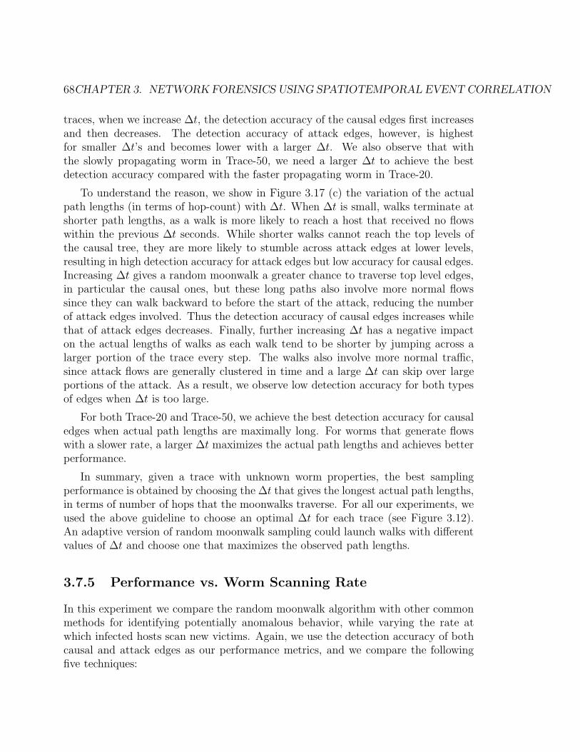
68CHAPTER 3. NETWORK FORENSICS USING SPATIOTEMPORAL EVENT CORRELATION
traces, when we increase ∆t, the detection accuracy of the causal edges first increasesand then decreases. The detection accuracy of attack edges, however, is highestfor smaller ∆t’s and becomes lower with a larger ∆t. We also observe that withthe slowly propagating worm in Trace-50, we need a larger ∆t to achieve the bestdetection accuracy compared with the faster propagating worm in Trace-20.
To understand the reason, we show in Figure 3.17 (c) the variation of the actualpath lengths (in terms of hop-count) with ∆t. When ∆t is small, walks terminate atshorter path lengths, as a walk is more likely to reach a host that received no flowswithin the previous ∆t seconds. While shorter walks cannot reach the top levels ofthe causal tree, they are more likely to stumble across attack edges at lower levels,resulting in high detection accuracy for attack edges but low accuracy for causal edges.Increasing ∆t gives a random moonwalk a greater chance to traverse top level edges,in particular the causal ones, but these long paths also involve more normal flowssince they can walk backward to before the start of the attack, reducing the numberof attack edges involved. Thus the detection accuracy of causal edges increases whilethat of attack edges decreases. Finally, further increasing ∆t has a negative impacton the actual lengths of walks as each walk tend to be shorter by jumping across alarger portion of the trace every step. The walks also involve more normal traffic,since attack flows are generally clustered in time and a large ∆t can skip over largeportions of the attack. As a result, we observe low detection accuracy for both typesof edges when ∆t is too large.
For both Trace-20 and Trace-50, we achieve the best detection accuracy for causaledges when actual path lengths are maximally long. For worms that generate flowswith a slower rate, a larger ∆t maximizes the actual path lengths and achieves betterperformance.
In summary, given a trace with unknown worm properties, the best samplingperformance is obtained by choosing the ∆t that gives the longest actual path lengths,in terms of number of hops that the moonwalks traverse. For all our experiments, weused the above guideline to choose an optimal ∆t for each trace (see Figure 3.12).An adaptive version of random moonwalk sampling could launch walks with differentvalues of ∆t and choose one that maximizes the observed path lengths.
3.7.5 Performance vs. Worm Scanning Rate
In this experiment we compare the random moonwalk algorithm with other commonmethods for identifying potentially anomalous behavior, while varying the rate atwhich infected hosts scan new victims. Again, we use the detection accuracy of bothcausal and attack edges as our performance metrics, and we compare the followingfive techniques:

3.7. REAL TRACE STUDY 69
• Random moonwalk selection: Pick the Z = 100 edges with the highestfrequency after performing 104 random moonwalks.
• Heavy-hitter detection: Find the 800 hosts that generated the largest num-ber of flows in the trace (the “heavy-hitters”). Randomly pick 100 flows betweentwo heavy-hitters. (We select 800 hosts as we know there are about 800 infectedhosts in the traces.)
• Super-spreader detection: Find the 800 hosts that contacted the largestnumber of distinct destination hosts (the “super-spreaders”). Randomly pick100 flows between two super-spreaders.
• Oracle selection: Assume an oracle that identifies the set of infected hostswith zero false positive rate. The oracle randomly selects 100 flows betweenthese hosts.
• Random selection: Randomly pick 100 flows from each trace.
Both heavy-hitter and super-spreader heuristics have been traditionally used todetect patterns of malicious activity in IDSes [83, 75].
10 20 30 50 75 1000
0.1
0.2
0.3
0.4
0.5
0.6
0.7
0.8
0.9
1
Worm inter−scan duration (second)
Atta
ck e
dge
accu
racy
Random walkOracle selectionSuper−spreader detectionHeavy−hitter detectionRandom selection
10 20 30 50 75 1000
0.1
0.2
0.3
0.4
0.5
0.6
0.7
0.8
0.9
1
Worm inter−scan duration (second)
Cau
sal e
dge
accu
racy
Random walkOracle selectionSuper−spreader detectionHeavy−hitter detectionRandom selection
(a) Attack edges (b) Causal edges
Figure 3.18: Detection accuracy vs. worm scanning rate. The X-axis represents theworm inter-scan duration. For example, a window of x = 20 means an infected hostgenerates an infection flow every 20 seconds.
As expected, the detection accuracy for attack edges decreases with an increasedworm inter-scan duration (Figure 3.18 (a)), since a worm that sends attack trafficat a slower rate will create fewer attack edges in the host contact graph. Randommoonwalk selection and oracle selection have similar performance and perform sub-stantially better than the other strategies. Perhaps surprisingly, heavy-hitter detec-tion performs even worse than random selection, as the heavy-hitter method is likelyto select servers, and most of the communication between servers is legitimate traffic.

70CHAPTER 3. NETWORK FORENSICS USING SPATIOTEMPORAL EVENT CORRELATION
The real success of the random moonwalk algorithm, however, is not in pickingattack edges. Rather it lies in its ability to extract causal edges from a large noisy hostcontact graph. This is evident from Figure 3.18 (b), where we notice that all othertechniques, including oracle selection, have a low detection accuracy for causal edgesacross all worm scanning rates. For attacks that spread at rates of one scan every 10-30seconds, the causal edge detection accuracy of random moonwalk selection is greaterthan 0.5, implying that roughly 50 out of the top 100 edges are always causal edges.This establishes the capability of finding the causal edges by globally correlating thehost traffic patterns for very stealthy attacks using the random moonwalk algorithm.On the other hand, the poor performance of even the oracle selection suggests thatdetecting infected hosts alone does not help extracting the causal edges to reconstructthe top level causal tree and trace back the worm origin.
3.7.6 Performance vs. Worm Scanning Method
C−100 C−500 A−100 A−5000
0.2
0.4
0.6
0.8
1
Acc
urac
y
Scan method 1Scan method 2
0.05 0.1 0.15 0.2 0.25 0.3 0.35 0.40.2
0.3
0.4
0.5
0.6
0.7
0.8
0.9
1
Fraction of hosts vulnerable (F)
Acc
urac
y
Causal edgesAttack edges
(a) (b)
Figure 3.19: (a) Comparing detection accuracy using worms with different scanningmethods using Trace-20. (b) Comparing detection accuracy using worms targetingdifferent fraction of vulnerable hosts F .
In this experiment, we study the effectiveness of random moonwalks using wormswith different scanning methods. Since many existing techniques identify worm scan-ners by looking at only flows sent to non-existent hosts [113, 44], a smart worm canevade such detection by carefully targeting only valid addresses. We therefore evaluatethe performance of our technique using two worms with different scanning methods.The first scanning method randomly scans only valid host addresses, while the secondmethod randomly scans both existent and non-existent host addresses with 50% ofhost address space being used. For both worms, an infected host starts scanning atthe rate of one attack flow every 20 seconds.

3.8. SIMULATION STUDY 71
Figure 3.19 (a) compares the detection accuracy of the top Z = 100 and Z = 500frequency edges for the two different worms. For both causal edges (represented byC-100 and C-500) and the attack edges (represented by A-100 and A-500), randommoonwalks achieve better detection accuracy for the “smart-scanning” worm, which isconsistent with our analytical study in Section 3.6.2. As random moonwalk samplingidentifies the subtle global tree patterns of worm propagation, instead of relying on thescanning behavior of each specific infected host, it is inherently more robust to otherworm scanning strategies [97, 113]. Such results are also encouraging for detectingthose worms that may evade detection techniques employed by many existing scan-detectors, which essentially use the number of connections to unused address chunksas a metric of interest [44, 88, 47].
3.7.7 Performance vs. Fraction of Hosts Vulnerable
This section studies the performance of the random moonwalk algorithm with differentfraction of hosts infected (i.e., we vary F ). With a greater number of hosts infectedby an attack, the degree of anonymity provided to the true attacker is also greater. Inthis experiment, we fix the worm scanning rate to be one attack flow per 20 seconds,and vary the fraction of hosts vulnerable F during each attack. Figure 3.19 (b) showsthe performance in terms of the detection accuracies of both causal edges and attackedges. Within the range of F = [0.05, 0.4], we observe that the detection accuraciesincrease as we increase the fraction of hosts infected. Empirically, our experimentsalso show that the detection accuracy increases for more slowly propagating attacks(e.g., one scan per 50 seconds) as they infect more hosts in the network along time.We plan to further quantify the impact of F on performance as future work.
3.8 Simulation Study
The goal of our simulation study is to evaluate the effectiveness of random moon-walks using different background traffic models of normal host communication. Ourhypothesis is that the simplified traffic model in our analytical study, where back-ground (i.e., normal) traffic, modeled as uniform scanning, is a worst case model forperformance of our algorithm. Realistic host contact graphs tend to be much sparser,meaning the chance of communication between two arbitrary hosts is very low sincehost connectivity patterns usually display locality in the set of destinations contacted.An epidemic “tree” structure will more easily stand out in such scenarios, and thusbe detected with higher accuracy.
In particular, we model the host connectivity patterns in terms of both the out-degree of normal hosts and the connection locality. The out-degree of each normal

72CHAPTER 3. NETWORK FORENSICS USING SPATIOTEMPORAL EVENT CORRELATION
Trace 1 2 3 4 5Host out-degree D |H| C < |H| |H| Power-law Power-lawConnection locality Uniform Uniform Power-law Uniform Power-law
Causal edge accuracy 0.506 0.472 0.546 0.616 0.614
Figure 3.20: Detection accuracy of causal edges using different background trafficmodels. “Power-law” means the controlled variable follows a power-law distribution(with a coefficient set to 3). “Uniform” means the controlled variable follows a uniformdistribution. |H| denotes the total number of hosts in the network, and C is a constantnumber smaller than |H|.
host is the size (denoted as D) of the contact set, which represents the set of desti-nations the host originates flows to under normal circumstances. Connection localityis modeled by assuming each host selects destinations preferentially (within the con-tact set) according to either a uniform or power-law distribution. Figure 3.20 liststhe background traffic generated using different combinations of the host out-degreeand connection locality. All the simulations run with |H| = 104 nodes for 3000 sec-onds of simulated time. We introduce worm attacks lasting 500 seconds with a fixedpropagating rate (A/B ' 7) that infect F = 0.1 fraction of hosts. Recall that A isthe connection rate of an infected host (including normal connections), and B is theconnection rate of a normal host. The resulting traces have about 106 total flows with1000 causal flows. For each trace, we perform 104 random moonwalks and computethe detection accuracy of causal edges among the returned top Z = 100 frequencyflows.
Overall, the random moonwalks achieve high detection accuracy across all back-ground traffic models. As expected, the power-law distribution of the host out-degreeresults in best performance as the corresponding normal host contact graphs aresparse. The power-law distribution connection locality has similar performance im-pact since each host tends to talk only to a few hosts within the contact set morefrequently, resulting in a relatively sparser host contact graph too. In contrast, uni-form destination selection with constant contact set size (i.e., D = C, or D = |H|)models random scanning background traffic, and yields the worst performance.
3.9 Random Moonwalks and Spectral Graph Anal-
ysis
Random Moonwalks exploits the global tree structure of attack propagation via aspecial way of sampling. While each next step in a walk is selected randomly from

3.9. RANDOM MOONWALKS AND SPECTRAL GRAPH ANALYSIS 73
the possible choices, the aggregated effect is not random, but deterministic in essence.We show in this section that the random moonwalk algorithm can be interpreted asperforming spectral graph analysis on a flow graph transformed from the host contactgraph that we defined earlier.
Spectral graph analysis is a popular method in social science and information re-trieval by exploiting the underlying graph structure of social or information entities.Such method studies graphs by their adjacency matrices or Laplacian matrices [22].The graph structures are shown to have tight relationships with the eigenvalues andthe eigenvectors of the associated matrix. Such properties can be used for clusteringor ordering nodes on the graphs. For example, existing works have performed linkanalysis [53, 81] to infer correlations among social network entities from their activitypatterns. In Web graph analysis, a number of eigenvector methods, such as Pager-anks [73] and HITS [50], have shown to be effective for identifying high quality pagesfor Web search.
Random moonwalks have strong connections with spectral graph analysis, in thatit can be regarded as a simulation method to compute the largest eigenvector of aspecial type of flow graphs. The underlying structure of a graph can be analyzedusing its largest eigenvector, in order to identify the existence of abnormal host com-munication patterns. In particular, the largest elements in the principal eigenvectorscorrespond to those abnormal events that directly or indirectly cause the structuralchanges of host communication graphs. Such a spectral analysis view offers betterinsight to the effectiveness of the algorithm under different attack models, and raisesopportunities for more optimized computation. We explain the details next, startingwith a flow graph model, with which we perform the spectral analysis.
3.9.1 A Flow Graph Model
Graphs are a common method for representing the relationships among various en-tities. In this section, we introduce a different graph representation to revisit thepreviously described random moonwalk algorithm. With this new graph model, ran-dom moonwalks can be interpreted as a sampling process for computing the largesteigenvector of the corresponding adjacency matrix.
We adopt the same notion of flows as discussed in Section 3.4. Similar to the hostcontact graph, the flow graph is defined as a direct graph Gf = 〈V, E〉. Each noden ∈ V on the flow graph corresponds to a network flow e = 〈u, v, ts, te〉. Therefore,in the rest of this section, we use n instead of e to denote a flow, and use the termnode and flow interchangeably.
Edges on the flow graphs capture the potential causal relations between flows.Given two nodes (i.e., two flows) n1 = 〈u1, v1, t
s1, t
e1〉 and n2 = 〈u2, v2, t
s2, t
e2〉, we define

74CHAPTER 3. NETWORK FORENSICS USING SPATIOTEMPORAL EVENT CORRELATION
Flow-ID Source Destination Start-time End-time
n1 A B 10 20
n2 E B 20 30
n3 B C 25 30
n4 B D 35 40
n5 B C 45 60
Figure 3.21: Five example network flows. A, B, C, D, and E are five different hostsin the network.
n1
n3 n4 n5
n2
A
B
C
D
EH
osts
10 20 30 40 50 60Time
(a) (b)
Figure 3.22: (a) The flow graph defined by the five network flows listed in Figure 3.21.(b) The host contact graph defined by the same five network flows.
a directed edge from n2 to n1, if v1 = u2 and te2 ≤ ts1 < te2 + δt, where δt is an inputparameter used to generate the flow graph. Intuitively, the directed edge from noden2 to n1 reflects a potential causal relationship between the two corresponding flows,meaning flow n2 might potentially be induced by flow n1. The parameter δt representsthe length of the time period, during which these two flows can be causally related.We shall see later that, for spectral analysis purpose, δt exactly corresponds to thesampling window size ∆t defined in the random moonwalk process, i.e., δt = ∆t.
As an example, Figure 3.21 lists five hypothetical network flows involving fivedifferent hosts A-E. Figure 3.22 (a) shows the corresponding flow graph defined bythe five network flows with δt = 20 seconds. We also plot the corresponding hostcontact graph (see Section 3.4) defined by the same five network flows in Figure 3.22(b). There are several significant differences between the two types of graphs. First,the main entities in the flow graph are network flows, while the main entities in thehost contact graph are states of hosts at different time stages. Second, since eachnetwork flow is associated with a unique start time and end time, we no longer needto encode time explicitly in the flow graph. Finally, a flow graph is defined withan additional input parameter δt, while in the host contact graph, the notion of the

3.9. RANDOM MOONWALKS AND SPECTRAL GRAPH ANALYSIS 75
sampling window size ∆t is meaningful only when we perform the random moonwalkson the graph. Thus, the host contact graph and the associated flow graphs have aone-to-many correspondence by varying the values of ∆t (hence δt).
Under this framework, it is easy to see how we can generate a flow graph, givenan already defined host contact graph. First, the edges on the host contact graph andthe nodes on the flow graph have a one-to-one correspondence. Once we determinethe sampling window size ∆t for random moonwalks on the host contact graph, wecan generate a corresponding flow graph, by inserting an edge from node (i.e., flow)n2 to n1, if it is possible for us to moonwalk from flow n2 to n1 in the host contactgraph.
3.9.2 Markov Random Walks on the Flow Graph
A flow graph defined using the above method can be considered as a Markov chainnetwork, where each node corresponds to a state in the Markov chain, and each edgecorresponds to a possible state transition. A random moonwalk on the host contactgraph thus corresponds to a Markov random walk on the flow graph. At each state, theprobability of transiting to a next downstream state will be evenly distributed amongall possible downstream states, due to the randomness of the next step selection in amoonwalk. With such Markov random walk interpretation, the normalized adjacencymatrix Af defined by a flow graph Gf , is a stochastic matrix whose row sums are all1. Let us now examine the spectral problem for the matrix Af , namely the solutionsto the equation:
Afx = λx
In order to ensure that random walks on the Markov flow graph Gf convergesto a unique stationary distribution π0, i.e., Afπ0 = λπ0, Gf needs to be irreducible,ergodic, and aperiodic [109]. However, because of the backward direction of time inperforming the walks, the above defined flow graph Gf is not irreducible. In otherwords, it’s possible to transit from a node (flow) ni to another node (flow) nj , if andonly if flow nj finishes earlier than the launch time of flow ni, not vice versa.
We can apply a commonly used graph transformation method [73] to overcomethe above problem without changing the random walk properties. The method worksby inserting an additional directed edge from every sink, i.e., node without outgoingedges, to every other node on the graph. It is trivial to see that the resulting graphG′
f meets all three requirements (irreducible, ergodic, and aperiodic), and is thereforeguaranteed to have a stationary distribution π0. Since each random moonwalk startswith a randomly selected flow on the host contact graph, a Markov random walk onthe original flow graph Gf is equivalent to a random walk on the transformed graphG′
f .

76CHAPTER 3. NETWORK FORENSICS USING SPATIOTEMPORAL EVENT CORRELATION
The stationary distribution π0 of the transformed Markov flow graph G′f , by its
definition, represents the probability of reaching every node in a global stable state.Such stationary distribution can be estimated by the simulation method where werepeatedly perform random walks on the flow graph. We have shown that randomwalks on the flow graph are equivalent to random moonwalks on the host contactgraph. One can therefore view random moonwalks on a host contact graph as a MonteCarlo sampling method to compute the stationary distribution of a correspondingflow graph. It has been shown that this stationary distribution equals to the largesteigenvector of the corresponding graph’s normalized adjacency matrix. The highestprobability flows being traversed in a random moonwalk therefore correspond to thosenodes with largest numerical values in the largest eigenvector. These flows, with highprobability, are the initial causal flows on the causal tree.
Such a spectral analysis view opens up the following two possibilities: First, thecomputation of a graph’s largest eigenvector is a well-known problem. We can system-atically explore more efficient methods to perform deterministic computation. Sec-ond, since the largest eigenvectors have strong connections with the underlying graphstructures, we may be able to gain more insights on how different attack models willimpact the flow graph structures and the detection performance consequently.
3.9.3 Deterministic Computation of Probabilities
A commonly used algorithm to compute a graph’s principle eigenvector is matrixpower method [38]. It finds the largest eigenvector π0 of a matrix A using iterativematrix multiplications.
The method starts with a random normalized vector z as a initial guess for π0. Wethen repeatedly multiply z with matrix A, and normalize the resulting vector y = Azas another new start z, until z eventually converges to π0. With matrix additionsand multiplications, the complexity of such power method in both space and timeis O(|E|2), where |E| is the total number of nodes (i.e., flows) on the graph. Suchquadratic complexity is very expensive in practice, as |E| is on the order of millionsfor even a small campus network with thousands of hosts.
To optimize both space requirement and computational effort, we may apply com-pression techniques such as [24] on very large graphs for more compact representa-tions, or exploit locality of matrix entries and efficient data structures for paralleland distributed computation [39, 14, 37]. We leave it as future work to extensivelyexplore these techniques for our specific application.
Empirically, the adjacency matrix Af of the original flow graph Gf can be usedto approximate A′
f of the transformed flow graph G′f in the matrix power method
to obtain a similar converged solution, especially for the highest ranked elements

3.9. RANDOM MOONWALKS AND SPECTRAL GRAPH ANALYSIS 77
5 10 15 20 25 30 35 40 45 5010
−6
10−5
10−4
10−3
10−2
10−1
100
Number of iterations
L1 n
orm
diff
eren
ceTransformed flow graphOriginal flow graph
10 20 30 40 50 60 70 80 90 1000
50
100
150
200
250
300
350
400
450
500
Causal flow ID (sorted by rank)
Ran
k in
the
larg
est e
igen
vect
or
Original flow graphTransformed flow graph
(a) (b)
Figure 3.23: (a) The convergence rate of the power method on both the transformedflow graph and the original flow graph. (b) The ranks of initial causal flows in thelargest eigenvector. The causal flows are sorted based on the rank obtained from theoriginal flow graph.
of our interest. Figure 3.23 (a) compares the convergence rate computed as the L1
norm differences of the resulting vectors after each iteration, using both the originalgraph and the transformed graph obtained from our campus network trace with anormalized attack rate of 1. Correspondingly, we show the ranks of the initial causalflows in the largest eigenvectors computed based on the two different flow graphs inFigure 3.23 (b). Using both graphs, the solutions converge quickly in about 20-30iterations. After 30 iterations, the resulting vectors computed from the original flowgraph converge more quickly due to the existence of sinks, which do not re-distributecumulated probabilities. Overall, the rankings of the initial causal flows on bothgraphs are very close to each other. Since the initial causal flows are more likely tobe sinks, they get slight higher probabilities from the original graph, and thus slightbetter ranks (i.e., lower ranks) as shown in Figure 3.23 (b).
Note that the adjacency matrix of the original flow graph is triangular because ofthe uni-direction of state transitions. As future work, we can exploit this property, to-gether with application semantics, to further optimize the power method computationfor our special case.
3.9.4 Sampling Based Approximation
In Section 3.6.3, we have estimated the number of samples (i.e., walks) required versesthe false positive rate of identifying the top level initial causal flows. A more generalquestion is how accurate we can approximate the largest eigenvector using the Monte

78CHAPTER 3. NETWORK FORENSICS USING SPATIOTEMPORAL EVENT CORRELATION
Carlo simulation method? Existing studies [13, 5] on the convergence rate of MonteCarlo algorithms have mostly focused on Web graphs. Given a total of n nodes onthe graph, to ensure a small variation of the target value for every node, the numberof samples required is on the order of O(n2), based on a rough estimate in [13]. Forthe forensics application of identifying initial causal flows, such complexity estimateis quite pessimistic, as our analysis and empirical results indicate that a small numberof samples can already achieve good detection accuracy.
Let us consider a flow graph, where each flow e has a deterministic probabilityof P (e). We would like to know how many moonwalks W are required to be 1 − ε
confident that the estimated probability ˆP (e) is within a predetermined margin oferror? We do so by estimating the standard deviation σ(e) of the correspondingrandom variable P(e). We have already shown in Section 3.6.3 that for large W , P(e)can be approximately by a normal distribution, so that
σ(e) =
√
P (e) × (1 − P (e))
W
To ensure σ(e) ≤ P (e)/k, where k is a parameter quantifying the error margin,we need
W ≤ (1 − P (e)) × k2/P (e)
The above estimate is general and applicable to all connected graphs. For our spe-cific application, there appear to be two factors that aid in the convergence rate of thesimulation process. First, the larger the deterministic P (e) is, the faster the conver-gence rate will be with a smaller W . The tree structured worm propagation suggeststhat the small number of initial causal flows are among the highest ranked flows inthe largest eigenvector, and thus have larger deterministic probabilities. Since theseare the flows that we care, a small number of walks can already closely approximatetheir probabilities. Figure 3.24 (a) plots the flow probability distribution computeddeterministically using the original flow graph, where there is a worm attack propa-gating at a normalized attack rate of 1. If we consider flows with P (e) ' 0.01 andk = 10, then we need about 104 moonwalks to approximate the probabilities of thesehigh ranked flows.
The second factor that contributes to the small number of samples is that in ourproblem, it suffices to identify only the relative orders of the highest ranked flows andthe algorithm will return a set Z of those flows. Suppose flow ei is a initial causalflow that we are interested in finding, where i is the rank of that flow in the largesteigenvector. We can relax the error margin by reducing k, as long as ˆP (ei) ≥ ˆP (ei+q)(q ≥ 1) is satisfied so that ei will be present in the returned set. Using the same flowtrace shown by Figure 3.24 (a), we plot in Figure 3.24 (b) the number of moonwalks

3.9. RANDOM MOONWALKS AND SPECTRAL GRAPH ANALYSIS 79
100
102
104
106
10−8
10−7
10−6
10−5
10−4
10−3
10−2
10−1
FLow ID (sorted)
Det
erm
inis
tical
ly c
ompu
ted
prob
abili
ty
100
101
102
103
104
103
104
105
106
107
108
Flow ID (sorted)
Num
ber
of w
alks
W
k = 20k = 10k = 5
(a) (b)
Figure 3.24: (a) Computed flow probability distribution with a worm attack. (b)Error margin parameter k vs. number of walks W .
W required by choosing different values of k. We observe that 104 − 105 walks canlead to relative tight bounds of error margins (k = 5, 10) for the set of highest rankedflows.
10 20 30 40 50 60 70 80 90 1000
50
100
150
200
250
300
350
400
450
500
Causal flow ID (sorted by order)
Ran
k in
the
outp
ut
Power method computation104 random moonwalks
10 20 30 40 50 60 70 80 90 1000
50
100
150
200
250
300
350
400
450
500
Causal flow ID (sorted by order)
Ran
k in
the
outp
ut
Power method computation105 random moonwalks
104 random moonwalks 105 random moonwalks
Figure 3.25: The ranks of initial causal flows computed deterministically comparedagainst the ranks computed using random moonwalk sampling.
As a performance summary, Figure 3.25 plots the ranks of the initial causal flowscomputed by different numbers of random moonwalks, compared with the ranks thatwere computed deterministically using power method on the same flow graph. Whileincreasing the number of walks to 105 reduces the variations of the sampled ranks,104 walks can already approximate the 50 initial flows with good accuracy, and thusexplains the overall high detection accuracies we have achieved with a small number

80CHAPTER 3. NETWORK FORENSICS USING SPATIOTEMPORAL EVENT CORRELATION
of samples.
3.9.5 Revisit the Effectiveness of Random Moonwalks
Given a connected graph, the first several largest eigenvectors of the adjacency ma-trix have a wide spectrum of applications, for example, identifying important nodesfor Web and social graphs [73, 50], segmenting images [61], and analyzing Internettopologies [36].
With an undirected graph, the largest eigenvector associated with the adjacencymatrix’ s principal eigenvalue inherently reflects the node degrees [36]. With a directedgraph, however, the largest eigenvector expresses more than just the node degree [36].The most similar usage to our application of largest eigenvectors on directed graphs,is Google’s Pagerank computation, where each element in the largest eigenvectorrepresents the eventual standing probability of a random Web surfer on the associatedWeb page.
Informally, two types of nodes (i.e. flows) are more likely to have higher ranks inthe largest eigenvector of a directed graph: (1) high out-degree nodes, and (2) nodesthat connect to high out-degree nodes. In the application of identifying the wormorigins, the high out-degree nodes correspond to network flows that are directly re-sponsible for creating a large number of new flows within the next ∆t interval. Again,∆t is the sampling window size of random moonwalks. The second types of nodes,the ones connecting to high out-degree nodes, are flows that indirectly generated alarge number of new flows. The notion of node out-degree is tightly associated withthe size of ∆t when we define the flow graph, so the node degree actually reflectsthe traffic rate induced by the flow into the network. Once we compute the largesteigenvector, those highest ranked flows are those that, directly or indirectly, inducea high aggregated traffic rate into the network subsequently. Such global effect isalso what we observe during the propagation of a worm attack, and exploited by therandom moonwalks.
In addition to degree, there is also a normalization factor that determines theranks of nodes. This normalization factor is due to the use of normalized adjacencymatrices. Intuitively, if there are a large number of flows that are equal likely togenerate a same set of new flows, then the probability of each one being the causalevent is small, resulting a low rank of every flow. Such normalization factor alsoexplains why random moonwalks are effective in catching the tree-structured wormpropagation patterns.

3.9. RANDOM MOONWALKS AND SPECTRAL GRAPH ANALYSIS 81
3.9.6 Impact of Attack Models on Performance
Since the largest eigenvector returned by random moonwalks depends on the struc-ture of the corresponding flow graph, the next question is how attackers can evadedetection, where the resulted flow graphs will look similar to a normal flow graph? InSection 3.7, we have shown how we can leverage the probability distribution of eachflow being traversed in random moonwalks, which also corresponds to the distributionof elements in the largest eigenvector, to detect the existence of a random scanningworm attack. In this section, we explore different worm spreading strategies to studythe applicable scope of our algorithm.
We take a simulated network trace as our background traffic, instead of usingthe real campus trace where there exists ”normal” active scanners already. Both thehost out-degree and contact set size follow power-law distributions, with the samesetup as described in Section 3.8. Our normal host communication model containsno pathological patterns. We inject attack traffic propagating via different strategiesinto the simulation trace, with a target of compromising approximately equal numberof hosts in the network for each attack. We then construct a flow graph using acomputed optimal ∆t.
Instead of performing random moonwalks, we deterministically compute the largesteigenvector of the resulting flow graphs using the matrix power method. The com-puted distributions and rankings are thus the theoretical optimal results that couldbe achieved with our algorithm. For each attack scenario, we compare the elementdistribution of the largest eigenvector resulted from worm traffic, against that withnormal traffic only. We also compute the causal flow detection accuracy out of the100 top frequency flows to study the algorithm performance.
Scanning Worms
We first re-visit the random scanning worm model as our baseline study, where weinject two different epidemic spreading worm attacks with different rates into thetrace. Each worm attack propagates with a fixed rate that infect F = 0.1 fraction ofvulnerable hosts. For the slow worm, it needs 2000 seconds to infect all the vulnerablehosts (see Figure 3.26).
Figure 3.27 plots the probability distributions of each flow being traversed in ran-dom moonwalks, both with and without the attacks. The probability distribution,which is also the largest eigenvector distribution, becomes much more steep due tothe worm traffic. With a faster propagating worm, we observe a more-biased dis-tribution compared with that of a slower worm. This is as expected, since for thefast propagating worm, each initial causal flow indeed introduces higher aggregatedtraffic rate into the network, resulting in larger weights in the corresponding largest

82CHAPTER 3. NETWORK FORENSICS USING SPATIOTEMPORAL EVENT CORRELATION
Worm type Random fast Random slow
Fraction of hosts infected 0.1 0.099Normalized attack rate 7 1Scan duration (second) 500 2000Optimal ∆t (second) 70 400Causal flow accuracy 57% 55%
Figure 3.26: The configurations of the two scanning worms.
eigenvector. We also note that the optimal ∆ used for random moonwalks is smallerin the presence of a faster worm, confirming our analysis in Section 3.7.
100
102
104
106
10−7
10−6
10−5
10−4
10−3
Flow ID (sorted)
Com
pute
d pr
obab
ility
of b
eing
trav
erse
d Without wormWith a fast random worm
100
102
104
106
10−7
10−6
10−5
10−4
10−3
Flow ID (sorted)
Com
pute
d pr
obab
ility
of b
eing
trav
erse
d Without wormWith a slow random worm
(a) (b)
Figure 3.27: Probability distributions with and without random scanning worms. (a)The normalized attack rate is 7. (b) The normalized attack rate is 1.
With deterministic computation, the detection accuracies of causal flows are 57%and 55%, for fast and slow worms. They are very close to what we have achievedwith 104 random moonwalks, which are 61.4% and 53%, respectively. These resultsre-iterate the effectiveness of our algorithm on random scanning worms, by leveragingthe non-uniform distributions of the corresponding largest eigenvectors.
Scanning Hosts
Section 3.9.5 discussed that high out-degree nodes are also likely to have higher ranksin the largest eigenvector of a flow graph. Next, we examine the scenarios where,in the lack of tree-structured epidemic spreading attacks, how single scanning hostswould impact the probability distributions.

3.9. RANDOM MOONWALKS AND SPECTRAL GRAPH ANALYSIS 83
Scanner type Random Scanner Fast hitlist scanner Slow hitlist scanner
Fraction of hosts infected 0.065 0.081 0.04
Normalized attack rate 90 7 3
Attack duration (second) 2000 2000 2000
Optimal ∆t (second) 400 400 400
Causal flow accuracy 0% 0% 1%
Figure 3.28: The configurations of the three scanners.
With a single host spreading an infection, it is more difficult to compromise asmany hosts as epidemic attacks. The single attack source has to be more aggressiveby (1) scanning for longer time, (2) increasing the scanning rate, or (3) increasing theaccuracy in hitting vulnerable hosts. We consider two types of scanning strategies.First, an attacker can randomly scan hosts with a more aggressive rate. While suchtype of attacks can easily be detected using existing methods such as [41, 83], we aremore interested in how they will change the probability distribution of the largesteigenvectors due to certain flows’ high out-degrees. Second, an attacker can pre-compile a list of vulnerable hosts, and scan these hosts only. The rate of such scanscould be slowed down relatively to evade detection, while still allowing the malicioushost to compromise a large number of hosts. We vary the rate of such scan in ourexperiment.
100
102
104
106
10−7
10−6
10−5
10−4
10−3
Flow ID (sorted)
Com
pute
d pr
obab
ility
of b
eing
trav
erse
d Without wormWith an aggressive random scanner
100
102
104
106
10−7
10−6
10−5
10−4
10−3
Flow ID (sorted)
Com
pute
d pr
obab
ility
of b
eing
trav
erse
d Without wormWith a fast hitlist scannerWith a slow hitlist scanner
(a) (b)
Figure 3.29: Probability distributions with and without random scanning hosts. (a)An aggressive random scanner (b) Scanners that spread infection via a pre-compiledhitlist.
Figure 3.28 shows the scanner configurations in the attacks we inject, and Fig-ure 3.29 plots the probability distributions due to the two different types of scanning

84CHAPTER 3. NETWORK FORENSICS USING SPATIOTEMPORAL EVENT CORRELATION
hosts. With an attack duration of 2000 seconds, none of the scanners can successfullyinfect all the vulnerable hosts.
Compared with the flow probability distribution without attacks, the probabilitydistributions with both the aggressive random scanner and the fast hitlist scannershow noticeable changes, mostly due to the probability increases for the first 100ranked flows. For the majority of lower ranked flows, there are no significant dis-tribution changes caused by the aggressive scanning behavior. Further investigationconfirms our hypothesis that, without the existence of epidemic structures in the flowgraph, the highest ranked flows are indeed mostly high out-degree ones because ofthe high scanning rate. The slow hit-list scanner, in contrast, does not change theprobability distribution as much due to its slow scanning rate. But it also failed toinfect as many hosts as the more aggressive scanners. These are expected results,as our algorithm in essence identifies higher aggregate traffic rates built up in thenetwork. For scanning attacks, the high out-degree flows are those flows precedingthe causal ones, instead of being the causal flows themselves. So random moonwalksdid not identify causal flows as high probability ones.
In summary, our algorithm can still identify the existence of aggressive scanners bydetecting the changes of flow probabilities, if not causal flows directly. The stealthyscanners that spread slowly with pre-compiled hitlists may evade detection, but arenot as efficient in compromising a large number of hosts. To detect these stealthyattacks, we might need additional information (e.g., attack signatures) or metrics(e.g., total number of hosts talked) for detection and forensic analysis.
Topologically Spreading Worms
Worms that spread topologically have caught greater attention recently [121]. Insteadof random scanning the address space, the topological spreading worms infect hostsvia pre-setup connections (e.g., use connections of P2P applications), or contact onlyknown neighbors (e.g., through email address books). Since they infect hosts withvalid addresses only, many techniques today such as [75, 82, 44, 88] will fail to detectthese attacks by looking at connections to un-used address space. We again considertwo types of strategies for spreading the infection topologically. For the first type ofworm, each infected host randomly scans its neighbors in the contact set 1 with ahigh connection rate. We call it a topological scanning worm. For a second type ofworm host, it sequentially contacts all the hosts in the contact set exactly once, andthen stops the attack to avoid being detected due to a high scan rate. We define itas a topological sequential worm.
Figure 3.30 shows the experiment set up for the two different types of topological
1The neighbor set of a host will be defined by specific application semantics.

3.9. RANDOM MOONWALKS AND SPECTRAL GRAPH ANALYSIS 85
Worm type Topological scanning Topological sequential
Fraction of hosts compromised 0.086 0.086Normalized attack rate 7 3Maximum scans per host +∞ Size of its contact-setAttack duration (second) 1000 625Optimal ∆t (second) 40 20Causal flow accuracy 50% 75%
Figure 3.30: The configurations of the two types of topological spreading attacks.
100
102
104
106
10−7
10−6
10−5
10−4
10−3
Flow ID (sorted)
Com
pute
d pr
obab
ility
of b
eing
trav
erse
d Without wormWith a topological scanning worm
100
102
104
106
10−7
10−6
10−5
10−4
10−3
Flow ID (sorted)
Com
pute
d pr
obab
ility
of b
eing
trav
erse
d Without wormWith a topological sequential worm
(a) (b)
Figure 3.31: Probability distributions with and without topological spreading worms.(a) Each infected host scans its neighbor set randomly. (b) Each infected host scansits neighbors exactly once.
worms. Because topological worms may not be able to contact the whole host addressspace, we additionally increase the fraction of vulnerable hosts to F = 0.5, assumingattacks that spread topologically have a higher success rate in infection attempts.Thus these attacks can eventually infect approximately 0.1 fraction of hosts, likeother worms. With a sequential worm, the scanning is more effective and infects allhosts that could be infected in 625 seconds, after which time the attack stops.
Figure 3.31 shows the probability distribution changes for the two different topo-logical worms. Both topological worms resulted in significant distribution changeslike random scanning worms, even though they contact only known neighbors in theircontact sets. The detection accuracies of causal flows are approximately equal or evenhigher than the case of random scanning worms. Perhaps surprisingly, the causal flowdetection accuracy for the topological sequential worm is much higher than the topo-logical scanning worm, even though the former propagates via a slower rate and does

86CHAPTER 3. NETWORK FORENSICS USING SPATIOTEMPORAL EVENT CORRELATION
Worm type Random hitlist Coordinated hitlist
Fraction of hosts infected 0.1 0.1Normalized attack rate 1 0.5Maximum scans per host +∞ 2Attack duration (second) 500 500Optimal ∆t (second) 100 400Causal flow accuracy 47% 6%
Figure 3.32: The configurations of the two hitlist spreading worms.
not perform as many scans. There are two reasons to explain the observation. First,the sequential worm hits vulnerable hosts more effectively with sequential scan, re-sulting in more effective propagation, and thus higher aggregate traffic rate earlieron. The second reason is the normalization factor in building the tree-structuredworm traffic patterns. We examine the false positive flows returned by the topologi-cal scanning worm, and found that many of them were repeated infection attempts.Thus random moonwalks have higher chance of diverging in the presence both causaland repeated infection attempts, and converge slower to causal flows. These results,again, confirm the effectiveness of random moonwalks in capturing the high aggre-gated traffic rates and the tree-structured traffic patterns, regardless of the attackscanning models.
Hitlist Spreading Worms
The topological sequential worm suggests that with the knowledge of known vulner-able hosts, attacks can spread more effectively with a relative lower scan rate. Weexamine two different types of epidemic attacks that spread by hitlist: (1) a randomhitlist worm that randomly scans hosts from the pre-compiled vulnerable host list, and(2) a coordinated hitlist worm that infects hosts using a divide and conquer strategy,with each infected host performing a maximal of two scans to only un-compromisedhosts.
Figure 3.32 lists the properties of the two different hitlist worms we examine.And we plot the flow probability distributions resulted from the attack traffic inFigure 3.33. With a hitlist, attacks can spread slowly in order to evade detection,while still infect all vulnerable hosts in a short period. Both attacks in our experimentspread with equal or even lower rate than an average normal host, and last for 500seconds only. For the random hitlist worm, we can still detect many causal flows byfocusing on the highest ranked flows in the largest eigenvector, since the worm stillincurs slight higher traffic rate with scan-like activity. The coordinated hitlist worm

3.9. RANDOM MOONWALKS AND SPECTRAL GRAPH ANALYSIS 87
100
102
104
106
10−7
10−6
10−5
10−4
10−3
Flow ID (sorted)
Com
pute
d pr
obab
ility
of b
eing
trav
erse
d Without wormWith a random hitlist worm
100
102
104
106
10−7
10−6
10−5
10−4
10−3
Flow ID (sorted)
Com
pute
d pr
obab
ility
of b
eing
trav
erse
d Without wormWith a coordinated hitlist worm
(a) (b)
Figure 3.33: Probability distributions with and without hitlist spreading worms. (a)Each infected host randomly scans a pre-compiled list of vulnerable hosts. (b) Infectedhosts scan in a coordinated way, with each one performing a maximal two scans toonly un-compromised hosts.
pushes the capabilities of our algorithm to a limit, since each infected host contactsonly two more hosts in addition to its normal traffic with a very slow rate. However,such type of worm, while conceptually simple, requires both accurate knowledge ofvulnerable hosts and coordination strategies among all infected hosts, and is thusharder to implement in practice. For this type of worm, we observe no flow probabilitydistribution change resulted from the attack traffic at all. Even in this case, ouralgorithm still successfully detects 6 initial causal flows out of the 100 top frequencyones, suggesting the great potential of the algorithm in identifying a wide class ofstealthy attacks.
We note that in our experiments, the list of vulnerable hosts are selected randomlyfrom the host population based on a given fraction. Once infected, each coordinatedhitlist worm will also randomly select a new vulnerable host to propagate the at-tack. In reality, certain hosts might be more vulnerable to a specific attack thanother hosts. For example, the SQL worm targets at systems running Microsoft SQLServer 2000 or Microsoft Desktop Engine (MSDE) 2000 only. In addition, attackerscan strategically infect servers only among the vulnerable host list during its initialpropagation. Because servers usually have a large number of incoming flows (i.e., ahigh fan-in rate), a causal attack flow to a server thus has a higher chance of evad-ing detection due to the random selection of flows among all candidates. Randommoonwalks may not be able to identify the initial causal flows for such attacks thatleverage the non-uniform host in-degrees on the host contact graph. One directionof future work is therefore to study the practicality of such attacks, and quantify thedetection performance degradation.

88CHAPTER 3. NETWORK FORENSICS USING SPATIOTEMPORAL EVENT CORRELATION
3.10 Distributed Network Forensics
Given the large number of ISPs and administrative domains (ADs) that make up theInternet, it is likely that Attacker Identification and Attack Reconstruction will haveto be deployed in a distributed fashion across the network. Each individual ISPs orADs may not have the complete host contact graph available. Even inside an AD,traffic auditing and forensics may not be deployed to cover the entire network. SomeADs will have very complete traffic auditing, others will have none, and many willaudit packets only at their borders and peering points with other ADs.
We formulate different scenarios in which partial and distributed deployment cantake place, identify challenges involved in each case, propose possible solutions, andevaluate the sensitivity of our algorithm to the extent of deployment and cooperationamong domains.
There are in general three scenarios where we have only partial information to per-form Attack Reconstruction and Attacker Identification, and may need cooperationsfrom distributed domains:
1. Traffic auditing is deployed in a large backbone network such as AT&T andSprint, but not the access networks connected to the backbone. In such case, weare likely to have the knowledge of a majority portion of the host contact graphwith a small portion of data missing. Because our proposed random moonwalkmethod relies on statistical sampling of the traffic traces, it has the potential toyield robust performance against missing data. The challenging questions are:(1) How does the amount of data missing affect the algorithm effectiveness? (2)What types of data missing will degrade the performance most? The answers tothese questions will help the ADs to strategically deploy traffic monitors insidetheir networks for best performance and costs. We discuss different situationswhere a small portion of data is missing, and quantify the impact of missingdata in Section 3.10.1
2. Two or more peering backbone networks or ADs independently deploy networkauditing. Due to trust and privacy issues (which will be further discussed inSection 3.12), data cannot not be shared across administrative domain bound-aries. In such scenario, a challenging question is: Can each AD perform forensicanalysis independently, and then collaborate with other ADs without expos-ing private data to each other? We propose and evaluate in Section 3.10.2 adistributed random moonwalk algorithm where no information about networkinternal traffic will be shared among different ADs.
3. Traffic auditing is deployed at small access networks, such as department orenterprise networks, to identify the attack entry point into the local network.

3.10. DISTRIBUTED NETWORK FORENSICS 89
In the lack of a globally visible attack structure, the task of Attack Identifi-cation and Attack Reconstruction becomes more challenging. In such case, wemight leverage additional information from network intrusion detection systems(NIDS) to obtain a good starting point for local traffic causality analysis. Forexample, since the scales of such networks will be relatively small, we may beable to afford more detailed traffic auditing and analysis, such as packet leveltraces, than the flow level graph that we explore. We may also exploit informa-tion such as the file system changes or system calls from host-based intrusiondetection systems. Many existing methods on host based causality analysis(e.g., [48, 49]) can also be used to reconstruct partial attack graphs using abottom-up approach. Thoroughly exploring these issues, however, is beyondthe scope of this thesis.
3.10.1 Missing Data Impact on Performance
First, we consider the scenario where traffic monitoring is deployed in a backbonenetwork with a small amount of data missing. Given that the majority of the hostcontact graph is available, most of the global tree structure of worm traffic will stillbe present, and potentially be identified by the random moonwalk algorithm.
There are two important questions regarding the algorithm performance in suchcase. First, how does the amount of data missing impact performance? Intuitively,the more missing data there are, the worse the performance would be. It wouldbe important to understand to what extent the results are still useful for tracingthe worm origin. Second, what portions of data missing will affect the algorithmeffectiveness most? Certain part of data might play a more critical role than otherdata in the process of identifying the initial causal flows. Presumably, if most of theinitial causal flows themselves are not audited or logged, it will be more challengingto carry further attack investigation.
To answer the above two questions, we perform a set of experiments with the samedata set used in Section 3.7. To simulate the partial deployment scenarios, we groupcampus IP addresses based on /24 prefix subnets, and select a subset of those as thesimulated access networks without traffic auditing. Based on the selected subnets, wesplit the whole network trace into two parts: backbone traffic and subnet traffic. Bothparts consist of internal traffic and border traffic. The internal traffic refers to thoseflow records, whose senders and receivers both reside at the corresponding network(s).This portion of traffic will not be observed outside the network domain. The bordertraffic refers to those flow records, whose senders or receivers only, locate inside thecorresponding network, but not both. Both the backbone and the access networkswill be able to observe such border traffic, should each side deploy traffic auditingindependently. Therefore, the portion of border traffic will be double counted as both

90CHAPTER 3. NETWORK FORENSICS USING SPATIOTEMPORAL EVENT CORRELATION
the backbone traffic and the subnet traffic.
0 50 100 150 200 2500
20
40
60
80
100
120
140
160
180
Subnet ID (sorted by hosts)
Num
ber
of h
osts
0 50 100 150 200 25010
0
101
102
103
104
105
106
Subnet ID (sorted by traffic)
Num
ber
of fl
ows
(a) (b)
Figure 3.34: (a) The distribution of the number of subnet hosts. (b) The distributionof traffic generated.
For the four hour CMU campus trace with 8040 internal hosts, there are in total219 /24 subnets. Figure 3.34 shows the the distributions of the number of hostsand the amount of traffic in terms of network flows generated from the 219 subnets.Given the non-uniform host and traffic distributions, we use the following methodsto select subnets, assuming traffic monitoring is not deployed at the selected subnetsto simulate different strategies of partial deployment:
• By traffic: Select subnets that generate the most amount of traffic.
• By host: Select subnets that have the most number of hosts.
• By infection time: Select subnets that contain those hosts who were infectedearliest in time. Those hosts correspond to the ones on the initial levels of thecausal tree.
Again, we choose the fraction of vulnerable host F = 0.1. The normalized wormrate that we introduce into the background trace is 1, with a worm inter-scan durationof 20 seconds. We use the detection accuracy of causal edges as our performancemetric. For each method, we first perform a case study by removing only a smallnumber of subnets from traffic auditing. We then gradually increase the number ofsubnets to remove in order to study the performance degradation verses the amountof traffic missing.

3.10. DISTRIBUTED NETWORK FORENSICS 91
Backbone Subnet
Total traffic (%) 78 43Total host (%) 97 3
Attack flows (%) 99 6Causal flows (%) 100 6
Figure 3.35: Remove 4 subnets by traffic.
Backbone Subnet
Total traffic (%) 70 69Total host (%) 92 8
Attack flows (%) 99 14Causal flows (%) 99 14
Figure 3.36: Remove 10 subnets by traffic.
1000 walks 10,000 walks0
0.1
0.2
0.3
0.4
0.5
0.6
0.7D
etec
tion
accu
racy
All traffic
Remove 4 subnets
Remove 10 subnets
Figure 3.37: Detection accuracy with trace data missing from the subnets that gen-erated most amount of traffic.
Remove Subnets by Traffic
In this case, we select a number of subnets that generated the most amount of trafficas the networks that are not monitored. Figure 3.35 and Figure 3.36 list the statisticsabout both the remaining backbone traffic and the subnet traffic, where we select4 subnets and 10 subnets, respectively. Note since the border traffic between thebackbone and the selected subnets will be counted in both traces, the sum of thebackbone and the subnet traffic will be greater than 100% of the original trace. Wealso show the percentages of attack flows and causal flows, observed by both thebackbone and the simulated access networks, counted in a similar way.
Figure 3.37 shows the detection accuracies of causal flows in such partial de-ployment scenarios, compared with the case where we have all the trace data avail-able. Interestingly, by removing the small number of subnets that generated the mostamount of traffic, we observe almost no performance degradation, though there is asignificant amount of traffic reduction in the remaining backbone trace (up to 30%reduction). In the case where we split off the flow records from 10 subnets, the ran-dom moonwalk algorithm achieves even slightly higher detection accuracies than theperformance with full data. To explain the reason, we examine the percentages ofhosts from the missing subnets, as well as the percentages of attack traffic including

92CHAPTER 3. NETWORK FORENSICS USING SPATIOTEMPORAL EVENT CORRELATION
Backbone Subnet
Total traffic (%) 98 43Total host (%) 84 16
Attack flows (%) 97 30Causal flows (%) 98 30
Figure 3.38: Remove 10 subnets by host.
Backbone Subnet
Total traffic (%) 92 51Total host (%) 73 27
Attack flows (%) 92 47Causal flows (%) 92 47
Figure 3.39: Remove 20 subnets by host.
1000 walks 10,000 walks0
0.1
0.2
0.3
0.4
0.5
0.6
0.7
Det
ectio
n ac
cura
cy
All traffic
Remove 10 subnets
Remove 20 subnets
Figure 3.40: Detection accuracy with trace data missing from the subnets that havethe most number of hosts.
causal flows left in the remaining trace in Figure 3.35 and Figure 3.36. We note thatthe selected subnets contain a small number of hosts only (less than 10%). Since ourattack model is random scanning worms, most of the attack traffic generated fromthe small percentage of hosts is directed at the rest of host population located in thebackbone network, and thus audited by the backbone as border network flows. Asa contrast, the majority of the high volume of internal traffic generated inside thesesubnets is mostly normal traffic. Removing such normal traffic does not impact theperformance significantly, and may even help concentrate random moonwalks towardattack flows and causal flows, resulting in slightly better performance.
Remove Subnets by Host
We then select subnets that have the most number of hosts as un-audited networks.Figure 3.38 and Figure 3.39 show the statistics about the traces where we split off 10subnets and 20 subnets by host, respectively.
Figure 3.40 shows the performance degradation without the selected subnets. Re-moving subnets that have the most number of hosts does not reduce the amount oftraffic seen at the rest of networks significantly, but has more negative impact on

3.10. DISTRIBUTED NETWORK FORENSICS 93
Backbone Subnet
Total traffic (%) 99 15Total host (%) 96 4
Attack flows (%) 99 8Causal flows (%) 99 12
Figure 3.41: Remove 4 subnets by infectiontime.
Backbone Subnet
Total traffic (%) 99 20Total host (%) 92 8
Attack flows (%) 99 16Causal flows (%) 97 22
Figure 3.42: Remove 10 subnets by infec-tion time.
1000 walks 10,000 walks0
0.1
0.2
0.3
0.4
0.5
0.6
0.7
Det
ectio
n ac
cura
cy
All traffic
Remove 4 subnets
Remove 10 subnets
Figure 3.43: Detection accuracy with trace data missing from the subnets that containhosts who were infected earliest in time.
the detection accuracies. This is again due to the scanning model of worm attacksto infect as many hosts as possible. With more hosts missing from partial backbonedeployment, we are more likely to miss a larger fraction of attack traffic generatedamong the large number of missing hosts. Indeed, from Figure 3.38 and Figure 3.39,we do observe more fraction of attack flows and causal flows missing from the re-maining trace, compared with the case where we split off subnets that generatedmost traffic. Such results suggest that for better detection performance, we shoulddeploy traffic monitoring at networks with more host populations than networks thatgenerate larger amount of network traffic.
Remove Subnets by Infection Time
In this case, we first sort all the infected hosts by their time of infection, and identifythose subnets that contain the hosts that were infected earliest, and split them offfrom the backbone correspondingly. For example, if host Ha, Hb, and Hc are the firstthree infected hosts, and they belong to subnet Sa, Sb, and Sc, then we split thesethree subnets off from the backbone and focus on the remaining data.

94CHAPTER 3. NETWORK FORENSICS USING SPATIOTEMPORAL EVENT CORRELATION
Figure 3.41 and Figure 3.42 list the statistics about the backbone traces and thesubnet traces, where we split 4 subnets and 10 subnets off by infection time, respec-tively. Figure 3.43 shows the detection accuracies in such partial deployment case,compared against the performance with full data available. We observe that whilethe backbone trace still keeps the majority of traffic and hosts, including attack flowsand causal flows, the performance does degrade slightly. We achieve similar detec-tion accuracies to the case where we remove almost 30% of hosts from the backbone,suggesting that removing subnets that contain the top level infected hosts generatesthe most impact on performance. Such results also have implications to how futurestealthy attacks might evade detection in forensic analysis. If traffic auditing is onlypartially deployed, then attackers can carefully spread an attack at its initial stage,to within the boundary of a network where no traffic auditing is deployed. After asufficient number of hosts are infected at this initial stage, the attackers can triggerall the infected hosts to start scanning toward the backbone, in order to launch afull-fledged attack.
Given the reduced detection accuracies with the top level infected hosts missing, animportant question is: Will we still be able to find relatively lower levels of the causaltree, which will be used to provide directions and hints for further investigation? Ifthe tree branches that we identify all point to hosts from a specific network, it isthen likely to be the location where the attack originates from. Figure 3.44 showsthe flow graph constructed from the 42 top-frequency flows after 104 walks on thetrace where we remove 10 subnets selected based on the top level infected hosts. If ahost involved in a flow belongs the subnets that we remove, we identify the host asfrom the missing subnets. We see there is a large tree branching structure emanatingfrom the missing subnets, providing a strong evidence that the attack might haveoriginated from the subnets without traffic auditing. Such results are encouraging forcatching even stealthy attacks, which may topologically spread the infection duringtheir initial phases.
Amount of Data Missing vs. Detection Accuracies
The previous subsections have discussed the cases where data is missing from onlya small number of subnets. In this section, we vary the number of subnets that willbe removed, and examine how performance degrades with the increasing amount ofmissing data, using the same three data selection methods.
Figure 3.45 (a) shows the detection accuracy of causal flows by varying the numberof subnets that will be removed from traffic auditing. As the number of subnetsdoes not directly reflect the amount of traffic missing, we also plot the detectionaccuracy vs. the amount of traffic missing from the campus trace in Figure 3.45 (b)correspondingly. Note all the infected hosts belong to the 100 subnets out of the total

3.10. DISTRIBUTED NETWORK FORENSICS 95
47
4589
21:06:21
5586
4057
20:56:20
281
20:42:12
7032
20:52:21
7791
20:49:20
3225
20:50:00
3535
20:50:41
691
20:51:40
4649
20:54:21
5770
20:55:40
5162
20:56:20
6583
20:59:41
1712
20:59:41
20:52:20 4133
20:52:40
7030
20:43:54
2184
20:47:10
247
20:52:41
3937
20:54:01
1882
20:53:01
4372
20:56:20
6739
20:57:40
5530
20:54:00
5401
20:55:01
3636
21:20:20
20:54:00
5703
20:56:40
1239
20:59:00
2168
20:56:41 22:10:01
2677
20:55:41
352
20:59:40
5472
20:57:00
22:18:21
3392
20:57:01
20:59:21
7805
20:59:40
21:21:00
1708
21:35:00
4950
21:46:21
1617
22:19:41
20:43:06
114
Missing subnets
Figure 3.44: Host communication graph with 42 top frequency flows after 104 walkson the trace where we remove 10 subnets selected based on the top level infectedhosts. Each circle represents a host with the number in the circle indicating the hostID. The ”Missing subnets” node represent all the hosts that belong to the subnetswithout traffic auditing. Solid arrows indicate successful infection flows (i.e. causaledges), while the dashed arrows represent unsuccessful infection attempts. The dottedarrows correspond to normal traffic flows. The number beside each arrow indicatesthe flow finish time.
219 ones, so there is no data point in the figures after we remove the 100 subnets byinfection time.
There are several observations we can draw from both figures. First, the per-formance degrades linearly with the increasing amount of missing data. Even withpartial trace available, random moonwalks can still identify part of the causal tree forout of band investigation. If administrators can predict the amount of traffic mon-itored or collected, they can estimate the potential performance degradation basedon the traffic auditing strategies. Second, removing subnets according to the trafficvolume has very small impact to performance overall. From Figure 3.45 (b), we seethat by removing subnets based on traffic, there is only 5% of performance decreaseeven in the case where 60% of traffic is missing. It suggests that traffic auditing canbe performed in a strategic way to achieve similar performance with reduced storagecost. On the other hand, as discussed before, removing subnets by host or infectiontime reduces the detection accuracies more significantly. As a further explanation,Figure 3.46 shows the percentage of causal flows missing with the increasing amountof trace data removed using the different methods. Indeed, removing subnets basedon top level infected hosts also eliminates many causal flows for forensic analysis,while the majority flows removed according to the traffic method are normal flows

96CHAPTER 3. NETWORK FORENSICS USING SPATIOTEMPORAL EVENT CORRELATION
0 50 100 150 2000
0.1
0.2
0.3
0.4
0.5
0.6
0.7
Number of subnets removed
Det
ectio
n ac
cura
cy
By trafficBy hostBy infection time
0 20 40 60 80 1000
0.1
0.2
0.3
0.4
0.5
0.6
0.7
Percentage of flows removed
Det
ectio
n ac
cura
cy By trafficBy hostBy infection time
(a) (b)
Figure 3.45: The causal flow detection accuracies with the decreasing amount of tracedata available. (a) Performance vs. the number of subnets selected. (b) Performancevs. the amount of traffic removed.
0 20 40 60 80 1000
10
20
30
40
50
60
70
80
90
100
Percentage of flows removed
Per
cent
age
of c
ausa
l flo
ws
rem
oved
By trafficBy hostBy infection time
Figure 3.46: Fraction of causal flows missing vs. the total amount of traffic removedusing the three different selection methods.
instead. Since our goal is to identify initial causal flows, the number of causal flowsin the trace directly impacts the detection accuracies.
Performance Summary
To summarize, with a small amount of data missing, random moonwalks can stillachieve similar detection accuracies, with only slight performance degradation. Theperformance decreases linearly with the amount of data missing, suggesting partialdata would still be helpful for forensic analysis. Since our attack model is randomscanning worms, it would be more effective to deploy traffic monitoring at networks

3.10. DISTRIBUTED NETWORK FORENSICS 97
with large host populations. Stealthy attacks may spread at un-audited networksduring its initial stage to degrade the detection performance most. Even in such case,however, random moonwalks can still identify lower levels of the causal tree branches,which point to the networks from where the attack originates for further investigation.
3.10.2 A Distributed Random Moonwalk Algorithm
In this section, we consider the scenario where two or more networks independentlyperform traffic auditing. For privacy and scalability reasons, data will not be shared,or stored at centralized repositories. Forensic analysis has to be performed collabo-ratively by all the participating networks in a distributed way.
Our algorithm for worm origin identification can be elegantly adapted to such adistributed deployment scenario, to incrementally perform random moonwalks amongmultiple networks or administrative domains (ADs). Figure 3.47 illustrates the highlevel concept of the distributed random moonwalks, where four networks collabora-tively perform the algorithm by exchanging intermediate results, as if the randommoonwalks are conducted on the entire big network made up by all four networks.
Figure 3.48 illustrates the detailed steps of the algorithm, using an example oftwo networks, referred as AD1 and AD2, respectively. Solid arrows represent thedirections of network flows, and dashed arrows represent the directions of randommoonwalks (in reverse to the flow directions). α, β, γ, and ω denote four differenttypes of flows. β and ω refer to those internal flows within the domains of AD1 andAD2, respectively. α refers to the set of flows originating from AD1 and terminatingat AD2, while γ refers to the set of flows originating from AD2 and terminating atAD1. For each iteration i in the algorithm, both AD1 and AD2 keep a counter ofhow many times each flow f is traversed inside its own domain, denoted as Ai(f) andBi(f), respectively. Given these notations, the algorithm works as follows.
Step 1: Each ADk independently starts Wk random moonwalks, with initial stepsrandomly chosen among flows initiated by hosts inside its own network.
In our example, AD1 starts W1 random moonwalks with initial steps selected fromthe flow set α and β. Similarly, AD2 starts W2 random moonwalks from the flow setγ and ω.
Step 2: For each AD, many walks will reach border flows whose senders are fromother domains. With only partial knowledge of the next step choices, such walks willbe stopped, while others will finish as regular.
In the two network example, AD1 will stop a walk once it reaches any flow in theset γ, and AD2 will stop a walk once it reaches any flow in the set of α.

98CHAPTER 3. NETWORK FORENSICS USING SPATIOTEMPORAL EVENT CORRELATION
Step 3: After each iteration i, the ADs exchange the frequency counts of borderflows. For every flow f that were initiated by a host from ADj′ and received by a hostfrom ADj, ADj shares the frequency count Ai(f) with ADj′, so that all the walks thatterminated at f prematurely could be continued within ADj′ in the next iteration.
In this example, AD1 shares with AD2 the frequency counts of all the flows in theset of γ. For simplicity, we denote the set of counts as Ai(γ). Similarly, AD2 shareswith AD1 the set of frequency counts Bi(α).
Step 4: At each next iteration i + 1 where i ≥ 1, every AD continues randommoonwalks only from border flows that were initiated by hosts inside its own network,and destined to hosts outside. The number of walks starting from each flow equalsexactly to the frequency count of the initial flow, which was exchanged during theprevious iteration.
In this example, suppose the frequency of a flow f ∈ α being traversed is B1(f)at AD2 after the first iteration. Then at the second iteration, AD1 will performA2(f) = B1(f) random moonwalks, all with f as their initial steps. Because thesource of f is located within AD1, AD1 now has a global view of all the possible nextsteps to continue those walks that stopped at f inside AD2 during the first iteration.
Step 5: All the ADs iteratively perform the operations from Step 2 to Step 4, untilthere are no flows to continue the walks globally. For each AD, the final frequencycount of a flow is the sum of of its frequency counts from all the iterations. The ADscan now share the final results for a global reconstruction, or individually performfurther investigation using the highest frequency flows as suspicious causal flows.
In our example, there are in total three iterations. For AD1, the final frequencycount of a flow f will be computed as
∑3i=1 Ai(f). Similarly, for AD2, the final
frequency count of a flow f will be∑3
i=1 Bi(f).
During the above process, we note that every walk after the first iteration is acontinuation of a path explored by other networks from the previous rounds. Thusthe distributed algorithm is exactly simulating the global random moonwalks in adistributed fashion. Due to the backward direction of time, it is guaranteed that allthe walks will terminate globally, if the ADs agree on a time boundary beforehand.The number of algorithm iterations is bounded by the maximum path length d of allthe walks, which can be estimated based on the knowledge of the total trace length,and the sampling window size ∆t.
To ensure that the initial steps of the distributed random moonwalks are chosenin a global randomized way, the number of walks, Wk, to be launch at ADk, shouldbe normalized based on the total number of flows that could potentially be selectedfrom ADk. Since the amount of traffic at a network might be used to infer sensitiveinformation about the customer populations or the network topologies, it can not be

3.10. DISTRIBUTED NETWORK FORENSICS 99
Figure 3.47: An AD graph illustrating the concept of incremental Attacker Identifi-cation and Attack Reconstruction.
shared or accessed by other ADs. Instead, all the ADs could agree on a normalizationfactor η for calculating the number of moonwalks launched from each network, where
For each ADk, Wk = η|E|k
.
Here |E|k represents the total number of flows initiated by hosts inside the networkof ADk. In our previous example, the number of moonwalks launched from AD1
W1 = η(|α| + |β|), and the number of walks performed by AD2 W2 = η(|γ| + |ω|).Since each AD independently performs random moonwalks within its own domain,Wk will not be released to the public.
The only information to be shared among different ADs, during the distributedalgorithm, is the frequency counts of border flows as intermediate results. No in-formation about internal hosts or traffic will be exposed. Due to the randomizationprocess along every step of the walks, a malicious AD should not be able to reverseengineer Wk from the shared counts. In addition, because the records of border flowsacross two different ADs will likely to be audited and logged by both networks any-way, exchanging the frequency counts of these flows leaks no additional informationabout either ADs or end users.
Figure 3.49 shows the detection accuracies of the distributed random moonwalkalgorithm applied to a two sub-network scenario simulated using the same CMUcampus network trace. Each sub-network has approximately equal number of hosts,and Figure 3.50 lists the traffic statistics of the two sub-networks. The attack trafficbounces across both networks by randomly scanning destination hosts among theentire network, with a normalized attack rate of 1 (i.e., each infected host performsone scan per 20 second). Each network starts random moonwalks independently, witha total of 104 walks launched from both networks. We observe that the causal flowdetection accuracies of both networks increase monotonically as the process goes on,and eventually converges. The final performance is comparable to what is achieved

100CHAPTER 3. NETWORK FORENSICS USING SPATIOTEMPORAL EVENT CORRELATION
AD1AD2
γγγγ
αααα
ββββ ωωωω
B1(γ)
B1(ω)
B1(α)A1(α)
A1(β)
A1(γ)
A2(α) = B1(α)
A2(γ)
A2(β)
B2(γ) = A1(γ)
B2(ω)
B2(α)A3(α) = B2(α)
A3(β)
A3(γ) B3(γ) = A2(γ)
B3(ω)
B3(α)
Figure 3.48: The distributed randommoonwalk algorithm.
0 5 10 15 200
0.1
0.2
0.3
0.4
0.5
0.6
0.7
Number of rounds
Cau
sal e
dge
dete
ctio
n ac
cura
cy
Network 1Network 2Network 1 and 2
Figure 3.49: The causal edge detection ac-curacy of the top 100 frequency flows us-ing the distributed random moonwalk al-gorithm.
Sub-network 1 Sub-network 2
Total traffic (%) 83 57Total host (%) 50 50
Attack flows (%) 75 74Causal flows (%) 77 73
Figure 3.50: Traffic statistics of the two sub-networks for distributed forensic analysis
with a unified global view of the network.
To estimate the communication cost, we consider the worst case scenario whereevery walk terminates at a different border flow during each iteration. Assume thereare in total W walks launched from all the networks, there will be maximally Wfrequency counts to be exchanged at each round. With a total of d iterations, theoverall communication overhead is W × d counts, distributed among all the partici-pating networks. In addition to the size of data in exchange, other costs include theoverhead of setting up secure channels for communication, for example, the cost ofauthentication and data encryption.
3.11 Random Sampling vs. Biased Sampling
We have shown that, by randomly sampling paths of host communication and corre-lating the traversed flows, we can effectively identify the top level causal tree of a wideclass of worm attacks. In this section, we explore variations of our algorithm, wherewe may strategically guide walks toward certain flows, or incorporate knowledge of

3.11. RANDOM SAMPLING VS. BIASED SAMPLING 101
compromised hosts output by the local intrusion detection systems (IDSes).
We discussed in Section 3.10.1 that a small number of hosts may generate a signif-icant fraction of total traffic. Consequently, we are more likely to select those normalflows as our initial steps by the “randomness” of the selection, taking more hops toreach the causal tree. Without the knowledge of compromised hosts, a simple heuris-tics to speedy the convergence of moonwalks is to start the walks from as many hostsas possible, since a potential target of a worm is to infect a large number of hostseventually. In our implementation, we set a counter for each host on the number oftimes it being selected as a starting point, and set a maximal threshold to bound thecounter. We define this heuristic as the maximum coverage rule.
Alternatively, suppose we have the perfect knowledge of the list of the compro-mised hosts after an attack, then the moonwalks can be guided toward these infectedhosts to achieve better performance in potential. We consider the following set ofalgorithm variations in this case:
• Initial step rule: We can start moonwalks from flows initiated by the knowncompromised hosts only.
• Next step rule: When selecting a next step in the path, prefer flows initiatedby a compromised host than by a normal host.
• Rank adjust rule: After performing the moonwalks, adjust the flow ranks bylowering the ranks of those flows not initiated by a compromised host.
We evaluate the impact of these rules on performance using the same campusnetwork trace, introducing different rates of artificially injected worm attacks. Again,we use the computed optimal ∆t to perform 104 moonwalks for each case, and repeateach run 5 times.
Figure 3.51 compares the causal flow detection accuracies resulted from the dif-ferent heuristics. Interestingly, the additional preferences in selecting the initial stepshave no substantial impact on performance. The maximum coverage rule outperformsthe default random moonwalk algorithm with marginal accuracy increase, suggest-ing that the default random moonwalks can already cover a large number of hostsquickly due to the random selection of next step hops. Because of the attack’s randomscanning model, most of the walks are also likely to be directed to infected hosts atsome point, resulting in similar effect as starting the walks from compromised hostsonly. However, biasing walks toward compromised hosts along the entire paths doesindeed improve the detection accuracy significantly. The reason is that by favoringflows initiated from infected hosts, moonwalks will more easily stay on the causal treeand converge to the initial causal flows. Adjusting the flow ranks after moonwalks

102CHAPTER 3. NETWORK FORENSICS USING SPATIOTEMPORAL EVENT CORRELATION
10 500
0.1
0.2
0.3
0.4
0.5
0.6
0.7
0.8
0.9
1
Worm inter−scan duration (second)
Det
ectio
n ac
cura
cy o
f cau
sal f
low
sBaseline
Maximum coverage rule
Initial step rule
Next step rule
Rank adjust rule
Figure 3.51: Detection accuracy achieved with different heuristics. “Baseline” refersto the default random moonwalk algorithm without heuristics.
can also lead to big performance improvement by removing those high ranked normalflows that are received by hosts on the top levels of the causal tree.
In summary, the knowledge of compromised hosts has a great potential to improvethe detection performance. Such information can be obtained from the output oflocal IDSes to strategically guide the selection of next steps for further enhancing thecapabilities of random moonwalks.
3.12 Discussion and Future Work
The previous sections have explored algorithmic issues of identifying the origin ofepidemic spreading attacks and the initial causal flows, both in centralized and dis-tributed scenarios. In practice, deploying an Internet-scale forensic analysis systemfor Attacker Identification and Attack Reconstruction is a non-trivial task. Therewill be a number of challenges as a result of the sheer scale of the Internet traffic andthe need for cooperation between different service providers. Next, we discuss someof the challenges that exists in the system deployment and their implications, andoutline future research directions.
a) A tremendous amount of data would be required to represent the complete hostcontact graph of the Internet. Our proposed method for identifying attack propagationpaths relies on a network auditing system to log end host communication records. Tobound the amount of audit data a network might observe, let us assume that a majorISP has O(100) POPs, and each POP has 10 Gbps capacity towards the middleof the ISP’s network. The total amount data flowing through the network couldthen be 102 POPs/ISP × 1010 bits/sec/POP = 1012 bits/sec. Now, supposing an
3.12. DISCUSSION AND FUTURE WORK 103
average packet size of 1000 bits and an average flow of 10 packets, that would be1012 bits/sec /(101 packets/flow × 103 bits/packet ) = 108 flows/sec.
So, if we wished to store a record for each flow sent over the network, it wouldrequire 108 flow records/sec ×102 bits/flow record = 1010 bits/sec , i.e., 10 Gbps forthe ISP or 1% of the overall network capacity (100× 10 Gbps). In order to keep onehour of data, the storage obligation for the ISP would be roughly 450 GB to storethe compressed data (assuming a 10 fold compression rate), distributed among thePOPs.
Thus the sheer volume of the data to be collected, stored and analyzed representsa problem of scalable and efficient data collection and analysis, but the quantitiesinvolved are not inconceivable.2 We also note that by the time a worm infectionbecomes so pervasive, that the induced traffic potentially outpaces these logging ca-pabilities, the records most important for finding the attack origin, namely those closeto the origin, have already been recorded.
b) The complete host contact graph for the entire Internet will not be available.As we discussed in Section 3.10, it is likely that auditing and forensic analysis will bedeployed in a piecemeal fashion across the Internet. Our eventual goal is to realize afederated Dragnet system, where each network or AD deploys the Dragnet monitorsand agents to cooperatively perform the attack investigation.
On the algorithmic side, our proposed random moonwalk method relies on sta-tistical sampling of the traffic traces, making it intrinsically robust to many kinds ofmissing data. As shown in Section 3.10.1, even when critical data is systematicallymissing, the method still produces a partial causal tree that can be used as a basis forfurther out-of-band investigation. The study about the missing data impact on per-formance and the distributed random moonwalk algorithm presented in Section 3.10are only our initial efforts toward this direction. There are also system issues to besolved for a real deployment.
Similar to single-packet IP traceback [94], we also envision an architecture inwhich distributed collection points log flow records and corresponding timestamps.In addition to the source and destination IP addresses, each flow record contains anidentifier for distinguishing two flows between the same source and destination atroughly the same time, for which we can use, e.g., the 13-bit identifier field of theinitial packet in the flow in the case of IPv4. Though this is not strictly necessary,it permits us to relax the degree of clock synchronization necessary among collectionpoints and can improve the accuracy of our search. At each individual collection point,we require two causally related flows be logged in their causal order and timestampedwith a common clock.
2Today, 500 GB of disk space costs $500 to $1,000.

104CHAPTER 3. NETWORK FORENSICS USING SPATIOTEMPORAL EVENT CORRELATION
With multiple networks or ADs collaborating with each other interactively, wealso need architectural support to share intermediate results in a reliable way. Suchdata exchange could be realized either by a ”push” mode, or by a ”pull” mode whereADs set up distributed repositories for flow record querying. In either case, onlyauthorized ADs should be able to access records in an authenticated way. And weneed mechanisms to detect misbehaving ADs in order to enforce the correctness ofthe analysis results.
c) Privacy concerns must be addressed. Issues of trust and cooperation betweendomains raise challenges with respect to protecting both domain proprietary infor-mation and end user privacy. It is particularly important to prevent the executionof queries that can either retrieve an arbitrary part of the entire host contact graphrecorded by an AD (hence leaking business data about the AD) or read out all flowsto or from an arbitrary host (hence violating the privacy of a normal host).
Even though our distributed algorithm requires information sharing/querying ononly border flows, misbehaving ADs can collaborate to infer the traffic patterns of aparticular victim AD. In addition, the frequency counts of border flows might createa covert channel for inferring network traffic or routing properties, especially in theexistence of multiple information channels among different ADs. Future work includeexploring the privacy implications of such data sharing, as attackers can carefully crafttraffic patterns to create covert channels that may disclose sensitive information.
The creation of a distributed network auditing service will also serve as a practicalapplication of work by ourselves and other researchers to develop techniques that limitthe disclosure of private information without compromising the amount of usefulinformation retrieved, and without adding too much communication overhead.
d) The security of the auditing system itself must be maintained. If data is to beuseful to law enforcement authorities, the auditing system must be constructed tomaintain a “chain of custody” that can convince a jury that the data cannot havebeen tampered with after being collected. It must also be impossible for an outsideattacker to “frame” an uninvolved host by creating traffic that implicates the host.Further, the auditing system itself will likely become a favorite point of attack. Itmust be defended against attackers who might first DoS attack the auditing system,then launch attacks without running the risk of detection.
e) There are a wide range of other types of attacks. Our approach is effective forthe class of attacks that propagate via “tree” structured communication patterns.Future work includes the development of algorithms to perform post-mortem analysisof a larger class of attacks. Our current implementation assumes that the semanticdirection of the flow is consistent with the network notion of flow directionality. At-tacks may try to obfuscate the notion of causality among network flows. As futurework, we can explore ways to make the algorithm robust to such attacks.

Chapter 4
Related Work
This chapter discusses related work in two parts. In the first part, we survey variousapproaches for leveraging distribution information and correlation mechanisms. Whilethese efforts are in general related with both applications we study, there is alsoapplication specific related work, which we will present in the second part.
4.1 Distributed Security Architectures
Spatiotemporal event correlation exploits sequences of events distributed across bothtime and space. Leveraging information gathered from distributed multiple measure-ment points, however, is not a new approach itself. Many researchers have noticedthe potential of the collective approaches in security, especially for intrusion detectionand anomaly detection in different contexts.
A lot of efforts have focused on the architectural issues in system design, so thatevents and alerts from distributed monitors could be audited and effectively synthe-sized. EMERALD (Event Monitoring Enabling Responses to Anomalous Live Distur-bances) [79], DIDS (Distributed Intrusion Detection System) [92], CSM (CooperativeSecurity Managers) [110], and AAFID (Autonomous Agents For Intrusion Detec-tion) [6] are independently proposed distributed architectures for intrusion detectionand response. They all use local monitors or agents to collect and filter suspiciousevents and anomaly reports from a variety of sources (network packet traces, SNMPtraffic, and system logs, etc.), watching multiple network links and tracking user activ-ity across different machines. The architectures provide both communication methodsfor monitors to exchange locally detected information and coordination methods toorchestrate various components of the systems. In particular, both EMERALD andAAFID aggregate alerts hierarchically, via different service layers or data collectioncomponents. In DIDS, local monitors perform data collection and reduction, then the
105

106 CHAPTER 4. RELATED WORK
generated alerts are analyzed by a centralized rule-based expert system. As a con-trast, CSM uses a peer-to-peer way to communicate among individual hosts without acentralized director. Our works starts with a similar motivation, but more focuses ona specific approach of correlating the distributed events, while these systems targetto provide the infrastructures useful for configuring distributed intrusion detectorsand combining alarms from them. We envision the spatiotemporal event correlationapproach to be complementary to these effort, not as a replacement of the existingarchitectures that provide global observation sharing.
4.2 Alert Correlation
Correlating different types of audit logs and alerts is another active area to exploitdistributed information for security. Abad et al. [3] have proposed to correlate het-erogeneous types of logs (e.g., system calls and network traffic) using both signature-based method and data mining method. Compared with using a single type of logs,their system can increase the detection accuracies.
In the same area, many researchers have proposed various statistical learning tech-niques to correlate INFOSEC (information security) alerts. Valdes and Skinner [103]propose a probabilistic-based correlation method using similarity measures of alertattributes. Follow up work [4] presents a case study of their deployment experienceon correlating heterogeneous sensor data with live traffic to reduce alert volumes. Qinand Lee [80] have developed a statistical framework to causally analyze sequences ofalerts for constructing attack scenarios, where low level alerts are aggregated andprioritized for time-series analysis.
There are also many other approaches that correlate sequences of alerts for an-alyzing attack scenarios. In [23, 69, 68], the correlations are performed by definingrules and relating alerts through pre-conditions and post-conditions. The assumptionis that the consequences of earlier attacks have a strong connection with the prereq-uisites of later attacks, since the earlier attacks are usually launched in preparationfor the later ones. Noel et al. [70] propose a signal analysis method to correlate se-quences of alerts by reasoning distances on attack graphs constructed with additionalvulnerability analysis to reduce the online processing overhead. Another approachproposed by Debar and Wespi [27] defines an architecture to correlate alerts throughboth backward-looking method (to reason about duplicate alerts) and forward-lookingmethod (to reason about consequence alerts), and then to aggregate them with pre-defined rules into attack scenarios.
Other efforts of correlating alerts include M-correlator [78], where a stream ofsecurity alerts are ranked and clustered into a consolidate incident stream for fur-ther analysis, and M2D2 [66], where the authors propose a formal data model for

4.3. RELATED WORK TO SEURAT 107
integrating different types of information into intrusion detection.
Compared with these alert correlation techniques, our approach tries to correlatesystem state transitions defined as low level events, rather than the results of localintrusion analysis. As such, spatiotemporal event correlation can potentially identifymore anomalous events that look normal from local monitors, and also detect thelack of normal patterns. Secondly, most of these approaches focus on temporallycorrelating alert sequences (though [3] discusses the advantages of spatial correlationin their paper), while our approach uses correlation techniques to learn both thetemporal and spatial pattern of host state transitions globally. Finally, this thesiswork currently focuses on correlating information gathered by homogeneous monitors(specifically, the file system change monitors and network flow monitors), rather thanheterogeneous types of logs that are exploit by many these existing methods. Asfuture work, we may enhance our work to include different type of measurement datato represent individual host states.
4.3 Related Work to Seurat
In the area of anomaly detection, Seurat uses file system updates to represent a hoststate change. File system updates have been known to be useful information for in-trusion detection. Tripwire [101], AIDE [57], Samhain [85] are well-known intrusiondetection systems that use file system updates to find intrusions. Recently proposedsystems such as the storage-based intrusion detection systems [77] and some com-mercial tools [76] support real-time integrity checking of file systems. However, allof them rely on a predefined rule set to detect anomalous integrity violation, whileSeurat automatically diagnoses the anomaly using learning based correlation acrosstime and space.
Several learning-based approaches to intrusion detection have been proposed toavoid the tedious task of defining detection rules and to spot new types of attacks. Forexample, Warrender et al. [108] used various machine-learning techniques to modelnormal system-call sequences. Ghosh et al. [35] applied Artificial Neural Networks tolearn anomaly and misuse detection models for system programs. Ko [51] employed amachine learning method (e.g., Inductive Logic Programming) to model valid opera-tions of a program, and Lee et al. [56] proposed a framework for data mining varioussystem audit data. Significant deviations from the automatically learned model indi-cates anomaly in those systems, similar to the techniques we used in Seurat. Theseexisting approaches, however,analyze only the temporal behavior of hosts or systems,while overlooking the advantages of spatially located events.
More related correlation approaches to Seurat are [105, 106] proposed by Wanget al. and [25] proposed by Dagon et al., whose authors have also noticed the value

108 CHAPTER 4. RELATED WORK
of spatial correlation. Wang et al. [105, 106] have applied a collective approach totackle misconfiguration problems. In their system, a malfunctioning machine candiagnose its problem by collecting system configuration information from other similarand friendly hosts connected via a peer-to-peer network. The work does not targetautomatic detection of anomalous events or patterns through correlation, but rather itaims at figuring out the cause of a detected problem. Dagon et al. [25] have proposed asystem to correlate observed events from honeypot machines for local worm detection.As honeypot machines are not used by actual users, any active network event issuspicious and will be correlated with the same event from other honeypot machinesto confirm the existence of worm propagation. Their approach therefore shares similarmotivations with alert-based correlation, while in our approach, we correlate bothnormal and abnormal events from regularly used machines to automatically detectthe existence of abnormal patterns.
The specific feature reduction techniques employed by Seurat, namely the waveletanalysis and the principal component analysis methods, have also been used in net-work security for anomaly detection and diagnosis. Except for being used for diseaseoutbreak detection in [119], wavelet analysis is also used in the domain of traffic anal-ysis to identify anomalous events that signal the onset of an attack [7]. Recently,Lakhina et al [54] have proposed a PCA based method to diagnose traffic volumeanomalies, where the high-dimensional space occupied by traffic measurements isseparated into disjoint subspaces correlating to normal and abnormal network condi-tions.
4.4 Related Work to Dragnet
In the area of network forensic analysis, we are not aware of any previous work that canautomatically pinpoint the origin of an epidemic attack or the initial causal infectionevents.
Our random moonwalk algorithm assumes that attack flows do not use spoofedsource IP addresses, since in the types of attacks we consider here, attack packets arerarely, if ever, spoofed. The overwhelming majority of attack traffic involved in thepropagation is initiated by victims instead of the original attacker, so using spoofedaddresses would only decrease the number of successful attacks1 without providingextra anonymity to the attacker.
If attackers do begin to use spoofed addresses, then traceback techniques [87, 16,9, 94, 58] could be used to determine the true source of each flow sampled by our
1For example, spoofed packets are useless for propagating an infection over TCP-based commu-nications, since the TCP handshake cannot complete, and spoofing addresses for UDP-based attacksin the presence of egress filters [32] results in the attack flows being discarded.

4.4. RELATED WORK TO DRAGNET 109
algorithm. Traceback alone, however, is not sufficient to track worms to their origin,as traceback determines only the true source of the packets received by a destination.In an epidemic attack, the source of these packets is almost never the origin of theattack, but just one of the many infected victims. Some method is still needed to findthe hosts higher up in the causal tree.
Among these IP traceback techniques, the single-packet traceback system of Sno-eren et al. [94] shares our requirement for an auditing system that logs the source anddestination of network traffic. While Snoeren’s scheme requires logging per packet ateach router on the packet’s path, our approach only requires logging per flow with farfewer logging elements, as flows need only be recorded by enough elements to permita query to find them and determine their causal orderings [55].
The notion of computer forensic analysis is not new, and has been previouslystudied in other context. King et al have proposed a set of mechanisms to reconstructa time-series attack events on a local host by observing OS-level objects [48, 49].Puchholz and Shields have also discussed possible approaches to identify origins of anattack by analyzing process level communication events [17, 18]. Both of their work,aims at local host causality analysis, and is not appropriate for large scaled networkforensics.
Recent work [118, 29] has also noticed the value of spatially correlating commu-nication events for detecting propagating attacks. Compared with our work, theseapproaches try to exploit attack specific behaviors. Because they either require de-tailed packet-level analysis or host state monitoring, their effectiveness is limited andcannot be applied in our application.
GrIDS (Graph-based Intrusion Detection System) [21] is another closely correlatedsystem that detects attacks by building a graph representation of network activitybased on the reports from all the hosts in a network. It correlates TCP/IP activityevents between hosts in the network to infer patterns of intrusive or hostile activ-ities based on predefined rules. GrIDS was designed to potentially identify attackpropagating paths like Dragnet, but with significant differences compared with ourapproach. First, to reduce data complexity, GrIDS uses a hierarchy to incrementallyfilter suspicious events with rules. It thus bears more similarity to alert-based cor-relation approaches. In addition, GrIDS targets mostly on-line detection of attacks,while our focus in Dragnet is to perform off-line analysis on a tremendous number ofnetwork flows automatically.
Other work on traffic causality analysis has mostly focused on detecting steppingstones, which is suggested [93] as a potential solution for worm origin identificationtogether with IP traceback. Just as we discussed that IP traceback cannot be usedto trace the origin of epidemic attacks, stepping stone techniques are not suitable forour objectives either.
110 CHAPTER 4. RELATED WORK
There have been in general two categories of approaches for detecting steppingstones. The first class of approaches focuses on content-based techniques [96] andthus require very expensive packet payload analysis. More importantly, they cannottrack down flows from polymorphic worms or worms that encrypt payloads. Theother class of approaches [120, 28] focus on correlating packet-level characteristics(e.g., inter-packet timings) to detect if multiple interactive connections are part ofa single attack session. However, using fine-grained packet timing characteristics forestablishing causality does not work for worm attacks which typically do not useinteractive sessions. Even in the context of detecting causality of interactive flows,such techniques still remain an active area of research especially with respect to therobustness of such timing correlations [12, 107]. In contrast, our work ignores packet-level characteristics and attack signatures, but instead focuses on establishing causalrelationships between flows by exploiting the globally visible structure of attacks.Thus the random moonwalk algorithm can potentially be agnostic to specific attackcontents, attack packet sizes, or port numbers used.
While our work does not depend on the generation of worm signatures, our ap-proach is complementary to these efforts [52, 47] as well as other efforts in detectingthe existence of attacks [65, 42, 44, 113] and traffic anomalies [8].
Finally, our method for correlating random walks is inspired by link analysis [53],where the authors infer correlations among social network entities from their activitypatterns.
Chapter 5
Conclusions and Future Work
In this chapter, we summarize our key contributions, discuss limitations, and proposeseveral new directions for future work.
5.1 Contributions
Network security is an arms race where new attacks will be invented trying to out-wit existing detection and analysis techniques. A wide variety of malicious attackstoday attempt to disrupt the normal functioning of a large number of hosts in theInternet. While many of these attacks are aggressive in their propagation, and theirmalicious patterns can be identified by known signatures individually, future suchattacks can potentially be much more stealthy to evade the detection of traditionaldetection systems deployed in isolation. Nevertheless, to effectively compromise morehosts eventually, these attacks are bound to display abnormal patterns that can bediscerned by correlating locally observed events in a global way. On the other hand,the increasing capacity and performance of networks and storage devices enable theefficient collection and storage of a huge amount of audit data distributed across thenetworks, making it possible to analyze large quantities of data globally. Our work ismotivated by both the trend that attacks are becoming more sophisticated, requiringglobal coordinated detection and analysis capabilities, and the technology trend ofvarious high performance devices.
The main contribution of this thesis is a general solution to reliably and effec-tively capture the abnormal patterns of a wide class of attacks, whose activities, whenobserved in isolation, may not seem suspicious or distinguishable from normal hostactivity changes. To achieve this goal, we present a spatiotemporal event correlationapproach that correlates events across both space and time, identifying aggregatedabnormal patterns to the host state updates. The key observation behind our ap-
111

112 CHAPTER 5. CONCLUSIONS AND FUTURE WORK
proach is that events introduced by malware in a network system often have bothtemporal and spatial locality. Abnormal events or patterns, which may not seemssuspicious locally, will stand out when they are correlated with events taking placeat different times and locations.
Based on the same high level concept, we instantiate the spatiotemporal eventcorrelation approach in two important security applications. The first application welook at is anomaly detection, where we develop a pointillist method to detect abnormalfile updates shared across multiple hosts (Chapter 2). The use of spatiotemporal eventcorrelation, in our prototype system Seurat, effectively detects both simulated attacksand various manually launched worms and viruses in real computer clusters. Thesecond application we study is network forensic analysis, where we propose a Dragnetframework for collecting and analyzing flow level traffic data (Chapter 3). In thisapplication, the spatiotemporal event correlation approach is exemplified as a randommoonwalk algorithm that identifies the initial successful infection flows for tracingepidemic attack origins. Our analysis, simulation based experiments, and real tracestudy have shown that the algorithm is effective in identifying the causal relationshipsbetween initial infection events for both fast propagating worms and a wide classof stealthy attacks. These results together, demonstrate the unique advantage ofspatiotemporal event correlation in both reducing false alarms and identifying globalabnormal patterns.
Compared with traditional correlation based approaches, a major challenge of spa-tiotemporal event correlation is the increased data scale and complexity by exploitingaggregated low level events. Yet, such challenge can be effectively addressed throughcompact event representations and efficient correlation algorithms, as demonstratedby the two applications studied in the thesis. In both cases, we reduce the datavolumes by orders of magnitude through statistical sampling and feature reductionmechanisms, demonstrating the feasibility of our approach in practice.
While the high level idea is the same, the two applications utilize different types ofevent data. The first application focuses on host file system updates, and the secondapplication examines network flows among end hosts. The specific data representationmethods and the correlation algorithms we develop in the two examples are also quitedifferent. In anomaly detection, the file update events are represented as featurevectors, and the correlation is performed by clustering vectors in a high dimensionalspace. For network forensic analysis, we represent communication events with a hostcontact graph, and the correlation is performed by sampling paths of network flows.All these suggest that spatiotemporal event correlation is a general approach, with nospecific constraints on the types of data to be correlated or the particular algorithmsto be used. We believe such an approach can be applicable to a wide range of securityapplications for identifying groups of related events with various semantics.

5.2. LIMITATIONS 113
5.2 Limitations
Because the power of spatiotemporal event correlation comes from an aggregatedview of events across both time and space, our approach will be most successful indetecting attacks that result in abnormal changes distributed at multiple hosts andlocations. Examples of such attacks include email viruses, worms, DoS attacks, andDDoS attacks. Our approach has similar limitations as many traditional approachesin detecting attacks that succeed only once or target only a few hosts in a the network.For example, attacks to a misconfigured FTP server that requires no root passwordmay not be able to duplicate at other machines. In the lack of global abnormalpatterns, the spatiotemporal event correlation may not be as effective to detect theseattacks.
In these single attack scenarios, however, spatiotemporal event correlation still hasits value by temporally correlating events for anomaly detection. However, humaninputs may be required in a feedback loop to eliminate the false alarms caused byunseen normal activities. When applied strategically, spatiotemporal event correla-tion may also detect single host attacks as outliers in the space dimension, providingstarting points for further investigation.
The detection of aggregated malicious behavior suggests that attackers may sig-nificantly slow down the rate of propagation, so that their infection events graduallyblend into the normal events to evade detection and identification. In particular, whenthere are only a single or a few malicious events during our detection or analysis win-dow, we may not be able to catch them through spatiotemporal event correlation.One solution is to use a larger detection window, waiting for more attack instances,which also suggests that the detection latency might be longer. However, we notethat by slowing down the rate of infection, the degree of attack virulence will also de-crease, compromising fewer machines and leaving more time for patching vulnerablehosts. It is interesting future work to understand to what extent we can still leveragethe power of aggregates for each specific application.
5.3 Future Work
In this section, we present research directions that are left open by this thesis.
5.3.1 Distributed Data Collection and Correlations
In the current prototypes of both Seurat and Dragnet, we rely on a centralized datarepository and analysis engine to store and correlate events collected from distributed
114 CHAPTER 5. CONCLUSIONS AND FUTURE WORK
monitors. Despite its simplicity, such centralized scheme has both scalability and pri-vacy issues. A distributed architecture to store and query data will potentially solveboth problems. Such architecture will consist of the following components: (1) dis-tributed monitors for collecting audit data in a coordinated way, (2) distributed repos-itories for indexing and storing audit trace, and (3) a distributed query mechanismto access event records efficiently. There are already a few initial attempts [2, 59, 98]from other research groups in this direction, focusing on specific types of data andscenarios.
The correlation algorithm can also be designed to analyze events in a distributedcollaborative fashion. In Section 3.10.2, we discussed how we can adapt the ran-dom moonwalk algorithm so that multiple administrative domains can collaborativelyperform worm origin identification without releasing private data. There are also ef-forts [60, 67] in sensor networks to aggregate information from distributed monitors.As future work, we can design and implement a generalized framework to support awide class of correlation algorithms at distributed locations.
5.3.2 Privacy Preserving Data Access Mechanisms
Our current correlation algorithms assume it is possible to directly access all theavailable data. In a larger scaled system with distributed repositories, event recordsmay not be shared straightforwardly to ensure user privacy. A number of existingsolutions such as [105, 95, 116] have proposed encryption-based and anonymity-basedmechanisms to share data with privacy preservation, but they only support limitedfunctionalities. It is a challenging problem for future research to effectively supporta wide range of correlation operations on event records without violating privacyguarantees.
5.3.3 Incorporation of Heterogenous Types of Data
In our thesis work, we consider mostly homogenous types of events for correlation.Existing work has shown that leveraging different types of audit logs can improve theaccuracy of attack detection [3, 66, 70]. In Section 2.5, we also explored a generalfeature vector space that supports different types of file update attributes, and haveshown that the use of additional feature attributes can help detect more types of ab-normal events. In the Dragnet system, the combination of intrusion detection resultswith the host contact graphs can also significantly improve the detection accuracy ofcausal flows (Section 3.11). These preliminary results are encouraging, and suggestthat, for future research, we can more effectively exploit the value of various types ofevents in the correlation process.

5.3. FUTURE WORK 115
5.3.4 Other Applications
Spatiotemporal event correlation is a general approach that can benefit a wide classof security applications. This thesis work has shown its effectiveness with two ex-amples. As future work, we can further generalize this approach to other scenarios,for example, network-based intrusion detection. In Seurat, we use file system updateevents to represent host state changes and thus require per-host based monitoring.With the increasing deployment of network traffic monitors, we can easily log boththe incoming and outgoing traffic of each host without interfering normal host func-tions. Such traffic data can be encoded to represent host state changes, and correlatedacross different machines for detecting malicious scans or backdoor traffic. As anotherexample, spatiotemporal event correlation can potentially be used to detect massivespam emails or the unauthorized use of email forwarding servers, by correlating boththe incoming and outgoing emails from a large number of users.

116 CHAPTER 5. CONCLUSIONS AND FUTURE WORK

Bibliography
[1] . PlanetLab. http://www.planet-lab.org.
[2] S. Seshan A. R. Bharambe, M. Agrawal. Mercury: Supporting Scalable Multi-
Attribute Range Queries. In Proc. of the ACM Sigcomm, 2004.
[3] C. Abad, J. Taylor, C. Sengul, Y. Zhou, W. Yurcik, and K. Rowe. Log Cor-
relation for Intrusion Detection: A Proof of Concept. In Proc. of the 19th
Annual Computer Security Applications Conference, Las Vegas, Nevada, USA,
December 2003.
[4] D. Andersson, M. Fong, and A. Valdes. Heterogeneous Sensor Correlation: A
Case Study of Live Traffic Analysis. Presented at IEEE Information Assurance
Workshop, June 2002.
[5] K. Avrachenkov, N. Litvak, D. Nemirovsky, , and N. Osipova. Monte Carlo
Methods in PageRank Computation: When One Iteration is Sufficient. Techni-
cal report, University of Twente, 2005.
[6] J. S. Balasubramaniyan, J. O. Garcia-Fernandez, D. Isacoff, E. Spafford, and
D. Zamboni. An Architecture for Intrusion Detection Using Autonomous
Agents. In Proc. of the 14th IEEE Computer Security Applications Confer-
ence, December 1998.
[7] P. Barford, J. Kline, D. Plonka, and A. Ron. A Signal Analysis of Network Traf-
fic Anomalies. In Proc. of ACM SIGCOMM Internet Measurement Workshop,
2002.
[8] P. Barford, J. Kline, D. Plonka, and A. Ron. A Signal Analysis of Network
Traffic Anomalies. In ACM SIGCOMM IMW, November 2002.
117

118 BIBLIOGRAPHY
[9] S. Bellovin, M. Leech, and T. Taylor. ICMP Traceback Messages. Internet
draft, work in progress, 2001.
[10] M. W. Berry, Z. Drmac, and E. R. Jessup. Matrices, Vector Spaces, and Infor-
mation Retrieval. SIAM Review, 41(2), April 1999.
[11] CERT Advisory CA-2003-20: W32/Blaster worm. http://www.cert.org/
advisories/CA-2003-20.html, 2003.
[12] A. Blum, D. Song, and S. Venkataraman. Detection of Interactive Stepping
Stones: Algorithms and Confidence Bounds. In Proc. of The Seventh Interna-
tional Symposium on Recent Advances in Intrusion Detection (RAID), 2004.
[13] L.A. Breyer. Markovian Page Ranking Distributions: Some Theory and Simu-
lations. Technical report, http://www.lbreyer.com/preprints.html, 2002.
[14] A. Z. Broder, R. Lempel, F. Maghoul, and J. Pedersen. Efficient Pagerank
Approximation Via Graph Aggregation. In Proc. WWW04, 2004.
[15] J. Browne. Probabilistic Design. http://www.ses.swin.edu.au/homes/
browne/probabilisticdesign.
[16] H. Burch and B. Cheswick. Tracing Anonymous Packets to Their Approximate
Source. In Proc. of USENIX LISA Systems Administration Conference, 2000.
[17] B. Carrier and C. Shields. Providing Process Origin Information to Aid in
Network Traceback. In Proc. of the 2002 USENIX Annual Technical Conference,
2002.
[18] B. Carrier and C. Shields. The Session Token Protocol for Forensics and Trace-
back. ACM Transactions on Information and System Security, 7:333–362, 2004.
[19] CERT Coodination Center. Overview of Attack Trends. http://www.cert.
org/archive/pdf/attack_trends.pdf, 2002.
[20] CERT Coordination Center. Overview of Attack Trends. http://www.cert.
org/archive/pdf/attack_trends.pdf, 2002.

BIBLIOGRAPHY 119
[21] S. Cheung, R. Crawford, M. Dilger, J. Frank, J. Hoagland, K. Levitt, J. Rowe,
S. Staniford-Chen, R. Yip, and D. Zerkle. The Design of GrIDS: A Graph-Based
Intrusion Detection System. Technical Report CSE-99-2, U.C. Davis Computer
Science Department, January 1999.
[22] F. R. K. Chung. Spectral Graph Theory. 1997.
[23] F. Cuppens and A. Miege. Alert Correlation in a Cooperative Intrusion Detec-
tion Framework. In IEEE Symposium on Security and Privacy, May 2002.
[24] G. E. Blelloch D. Blandford and I. Kash. Compact Representations of Separable
Graphs. In ACM/SIAM Symposium on Discrete Algorithms (SODA), 2003.
[25] D. Dagon, X. Qin, G. Gu, W. Lee, J. Grizzard, J. Levin, and H. Owen. Hon-
eyStat: Local Worm Detection Using Honeypots. In The 7th International
Symposium on Recent Advances in Intrusion Detection (RAID 2004), Septem-
ber 2004.
[26] H. Debar, M. Dacier, and A. Wespi. Towards a Taxonomy of Intrusion-detection
Systems. Computer Networks, 31(9):805–822, April 1999.
[27] H. Debar and A. Wespi. Aggregation and Correlation of Intrusion-Detection
Alerts. In Recent Advances in Intrusion Detection. Volume 2212 of Lecture
Notes in Computer Science, Springer-Verlag, 2001.
[28] D. L. Donoho, A. G. Flesia, U. Shankar, V. Paxson, J. Coit, and S. Staniford-
Chen. Multiscale Stepping-Stone Detection: Detecting Pairs of Jittered Inter-
active Streams by Exploiting Maximum Tolerable Delay. In Proc. of The 5th
International Symposium on Recent Advances in Intrusion Detection (RAID),
2002.
[29] D. R. Ellis, J. G. Aiken, K. S. Attwood, and S. D. Tenaglia. A Behavioral
Approach to Worm Deetection. In Proc. of the 2004 ACM workshop on Rapid
malcode (WORM), 2004.
[30] F-Secure. F-Secure Security Information Center. http://www.f-secure.com/
virus-info.

120 BIBLIOGRAPHY
[31] M. Faloutsos, P. Faloutsos, and C. Faloutsos. On Power-Law Relationships of
the Internet Topology. In ACM SIGCOMM, 1999.
[32] P. Ferguson and D. Senie. RFC 2267 - Network Ingress Filtering: Defeating
Denial of Service Attacks Which Employ IP Source Address Spoofing, 1998.
[33] E. Forgy. Cluster analysis of multivariante data: Efficiency vs. Interpretability
of classifications. Biometrics, 21(768), 1965.
[34] A. Gersho and R. Gray. Vector Quantization and Signal Compresssion. Kluwer
Academic Publishers, 1992.
[35] A. K. Ghosh and A. Schwartzbard. A Study in Using Neural Networks for
Anomaly and Misuse Detection. In 8th Usenix Security Symposium, 1999.
[36] C. Gkantsidis, M. Mihail, and E. Zegura. Spectral Analysis of Internet Topolo-
gies. In Proc. of Infocom, 2003.
[37] D. Gleich, L. Zhukov, and P. Berkhin. Fast Parallel PageRank: A Linear System
Approach. Technical report, Yahoo, 2004.
[38] G.H. Golub and C.F. Van Loan. Mattrix Computation. Johns Hopkins Univer-
sity Press, 2nd edition, 1989.
[39] T. Haveliwala. Efficient Computation of PageRank. Technical report, Stanford
University, 1999.
[40] R. Heady, G. Luger, A. Maccabe, and M. Servilla. The Architecture of a Net-
work Level Intrusion Detection System. Technical report, Computer Science
Department, University of New Mexico, 1999.
[41] L. T. Herberlein, G. V. Dias, Karl N. Levitt, Biswanath Mukherjee, J. Wood,
and D. Wolber. A Network Security Monitor. In Proc. of the 1990 IEEE
Symposium on Security and Privacy, 1990.
[42] A. Hussain, J. Heidemann, and C. Papadopoulos. A Framework for Classifying
Denial of Service Attacks. In Proc. of ACM SIGCOMM, 2003.
[43] I. T. Jolliffe. Principle Component Analysis. Spring-Verlag, New York, 1986.

BIBLIOGRAPHY 121
[44] J. Jung, V. Paxson, A. W. Berger, and H. Balakrishnan. Fast Portscan De-
tection Using Sequential Hypothesis Testing . In Proc. of IEEE Symposium on
Security and Privacy, 2004.
[45] M. Kamber. Data mining: Concepts and techniques. Morgan Kaufmann Pub-
lishers, 2000.
[46] G. H. Kim and E. H. Spafford. The Design and Implementation of Tripwire: A
File System Integrity Checker. In Proc. of ACM Conference on Computer and
Communications Security (CCS), 1994.
[47] H. A. Kim and B. Karp. Autograph: Toward Automated, Distributed Worm
Signature Detection. In Proc. of 12th USENIX Security Symposium, 2004.
[48] S. T. King and P. M. Chen. Backtracking Intrusions. In 2003 Symposium on
Operating Systems Principles (SOSP), 2003.
[49] S. T. King, Z. M. Mao, D. G. Lucchetti, and P. M. Chen. Enriching Intrusion
Alerts Through Multi-host Causality. In 2005 Network and Distributed System
Security Symposium (NDSS), 2005.
[50] J. Kleinberg. Authoritative Sources in a Hyperlinked Environment. In Proc. of
9th ACM-SIAM Symposium on Discrete Algorithms, 1998.
[51] C. Ko. Detecting Intrusions Using System Calls: Alternative Data Models. In
IEEE Symposium on Security and Privacy, May 2000.
[52] C. Kreibich and J. Crowcroft. Honeycomb – Creating Intrusion Detection Sig-
natures Using Honeypots. In Proc. of ACM HotNets-II, 2003.
[53] J. Kubica, A. Moore, D. Cohn, and J. Schneider. Finding Underlying Con-
nections: A Fast Graph-Based Method for Link Analysis and Collaboration
Queries. In Proc. of Twentieth International Conference on Machine Learning,
2003.
[54] A. Lakhina, M. Crovella, and C. Diot. Diagnosing Network-Wide Traffic
Anomalies. In ACM SIGCOMM, August 2004.
[55] L. Lamport. Time, Clocks, and the Ordering of Events in a Distributed System.
Communications of the ACM, 21:558–565, 1978.

122 BIBLIOGRAPHY
[56] W. Lee and S. J. Stolfo. A Framework for Constructing and Models for Intrusion
Detection Systems. ACM Transactions on Information and System Security,
3(4), November 2000.
[57] R. Lehti and P. Virolainen. AIDE - Advanced Intrusion Detection Environment.
http://www.cs.tut.fi/~rammer/aide.html.
[58] J. Li, M. Sung, J. Xu, L. Li, and Q. Zhao. Large-scale IP Traceback in High-
speed Internet: Practical Techniques and Theoretical Foundation. In Proc. of
IEEE Symposium of Security and Privacy, 2004.
[59] X. Li, F. Bian, H. Zhang, C. Diot, R. Govindan, and G. Iannaccone. MIND: A
Distributed Multi-Dimensional Indexing System for Network Monitoring. Under
submission, 2005.
[60] S. Madden, M. J. Franklin, J. M. Hellerstein, and W. Hong. TAG: A Tiny
AGgregation Service for Ad-Hoc Sensor Networks. In OSDI, 2002.
[61] M. Maila and J. Shi. A Random Walks View of Spectral Segmentation. In AI
and STATISTICS 2001(AISTATS), 2001.
[62] A. Moore. K-means and Hierarchical Clustering. http://www.cs.cmu.edu/
~awm/tutorials/kmeans09.pdf (available upon request), November 2001.
[63] D. Moore, V. Paxson, S. Savage, C. Shannon, S. Staniford, and N. Weaver.
Inside the Slammer Worm. IEEE Security and Privacy, 1:33–39, July 2003.
[64] D. Moore, C. Shannon, G. M. Voelker, and S. Savage. Internet Quarantine:
Requirements for Containing Self-Propagating Code. In Proc. of IEEE INFO-
COM, 2003.
[65] D. Moore, G. M. Voelker, and S. Savage. Inferring Internet Denial-of-Service
activity. In Proc. of 10th USENIX Security Symposium, 2001.
[66] B. Morin, L. Me, H. Debar, and M. Ducasse. M2D2: A Formal Data Model for
IDS Alert Correlation. In Recent Advances in Intrusion Detection, September
2002.
[67] S. Nath, P. B. Gibbons, S. Seshan, and Z. Anderson. Synopsis Diffusion for
Robust Aggregation in Sensor Networks . In ACM SenSys, 2004.

BIBLIOGRAPHY 123
[68] P. Ning, Y. Cui, and D. S. Reeves. Analyzing Intensive Intrusion Alerts Via
Correlation. In Recent Advances in Intrusion Detection. Volume 2516 of Lecture
Notes in Computer Science, Springer-Verlag, 2002.
[69] P. Ning, Y. Cui, and D. S. Reeves. Constructing Attack Scenarios through Cor-
relation of Intrusion Alerts. In Proc. of the 9th ACM Conference on Computer
and Communications Security, 2002.
[70] S. Noel, E. Robertson, and S. Jajodia. Correlating Intrusion Events and Build-
ing Attack Scenarios through Attack Graph Distances. In Proc. of the 20th
Annual Computer Security Applications Conference, December 2004.
[71] The Network Time Protocol. http://www.ntp.org.
[72] PacketStorm. Packet Storm. http://www.packetstormsecurity.org.
[73] L. Page, S. Brin, R. Motwani, and T. Winograd. The pagerank citation ranking:
Bring order to the web. Technical report, Stanford University, 1998.
[74] K. Park and H. Lee. On the Effectiveness of Route-Based Packet Filtering
for Distributed DoS Attack Prevention in Power-Law Internets. In ACM SIG-
COMM, 2001.
[75] V. Paxson. Bro: A System for Detecting Network Intruders in Real-Time. In
Proc. of 7th USENIX Security Symposium, 1998.
[76] Pedestal Software. INTACTTM. http://www.pedestalsoftware.com/
products/intact.
[77] A. Pennington, J. Strunk, J. Griffin, C. Soules, G. Goodson, and G. Ganger.
Storage-based Intrusion Detection: Watching Storage Activity for Suspicious
Behavior. In Proc. of 12th USENIX Security Symposium, Washington, DC,
August 2003.
[78] P. A. Porras, M. W. Fong, and A. Valdes. A Mission-Impact-Based Approach
to INFOSEC Alarm Correlation. In Recent Advances in Intrusion Detection,
September 2002.

124 BIBLIOGRAPHY
[79] P. A. Porras and P. G. Neumann. EMERALD: Event Monitoring Enabling
Responses to Anomalous Live Disturbances. In Proc. of the 20th National
Information Systems Security Conference, October 1997.
[80] X. Qin and W. Lee. Statistical Causality Analysis of INFOSEC Alert Data. In
Recent Advances in Intrusion Detection, September 2002.
[81] M. Richardson and P. Domingos. Mining Knowledge-Sharing Sites for Viral
Marketing. In Proc. of the eighth ACM SIGKDD international conference on
Knowledge discovery and data mining, 2002.
[82] S. Robertson, E. Siegel, M. Miller, and S. Stolfo. Surveillance Detection in
High Bandwidth Environments. In Proc. of the 2003 DARPA DISCEX III
Conference, 2003.
[83] M. Roesch. Snort - Lightweight Intrusion Detection for Networks. In Proc. of
USENIX LISA Systems Administration Conference, 1999.
[84] University of Oregon Route Views Project. http://www.routeviews.org.
[85] Samhain Labs. Samhain. http://la-samhna.de/samhain.
[86] SANS Institute. Lion Worm. http://www.sans.org/y2k/lion.htm, April
2001.
[87] S. Savage, D. Wetherall, A. Karlin, and T. Anderson. Practical Network Support
for IP Traceback. In Proc. of ACM SIGCOMM, 2000.
[88] S. E. Schechter, J. Jung, and A. W. Berger. Fast Detection of Scanning Worm
Infections. In Proc. of 7th International Symposium on Recent Advances in
Intrusion Detection (RAID), 2004.
[89] B. Schneier and J. Kelsey. Cryptographic Support for Secure Logs on Untrusted
Machines. In The Seventh USENIX Security Symposium, January 1998.
[90] Bruce Schneier. Attack Trends: 2004 and 2005. http://www.schneier.com/
blog/archives/2005/06/attack_trends_2.html.
[91] V. Sekar, Y. Xie, D. Maltz, M. K. Reiter, and H. Zhang. Toward a Framework
For Internet Forensic Analysis. In Proc. of ACM HotNets-III, 2004.

BIBLIOGRAPHY 125
[92] S. R. Snapp, S. E. Smaha, D. M. Teal, and T. Grance. The DIDS (distributed
intrusion detection system) prototype. In The Summer USENIX Conference,
pages 227–233, San Antonio, Texas, June 1992. USENIX Association.
[93] A. Snoeren. Public Review of ‘Toward a Framework for Internet Forensic Anal-
ysis’. In Proc. ACM HotNets-III, 2004.
[94] A. C. Snoeren, C. Partridge, L. A. Sanchez, C. E. Jones, F. Tchakountio, S. T.
Kent, and W. T. Strayer. Hash-Based IP Traceback . In Proc. of ACM SIG-
COMM, 2001.
[95] D. X. Song, D. Wagner, and A. Perrig. Practical solutions for search on en-
crypted data. In IEEE Symposium on Security and Privacy, May 2000.
[96] S. Staniford-Chen and L. T. Heberlein. Holding Intruders Accountable on the
Internet. In Proc. of the IEEE Symposium on Security and Privacy, 1995.
[97] S. Staniford-Chen, V. Paxson, and N. Weaver. How to Own the Internet in
Your Spare Time. In Proc. of 11th USENIX Security Symposium, 2002.
[98] K. Suh, Y. Guo, J. Kurose, and D. Towsley. Locating Network Monitors: Com-
plexity, Heuristics, and Coverage. In Proc. of Infocom, 2005.
[99] Symantec. Symantec Security Response. http://securityresponse.
symantec.com.
[100] Symantec. Symantec Internet Security Threat Report, Volume VI. http:
//enterprisesecurity.symantec.com/content.cfm?articleid=1539,
September 2004.
[101] Tripwire, Inc. Tripwire. http://www.tripwire.com.
[102] Trusted Computing Platform Alliance. Trusted Computing Platform Alliance.
http://www.trustedcomputing.org.
[103] A. Valdes and K. Skinner. Probabilistic Alert Correlation. In Recent Advances
in Intrusion Detection. Volume 2212 of Lecture Notes in Computer Science,
Springer-Verlag, 2001.

126 BIBLIOGRAPHY
[104] D. Wagner and D. Dean. Mimicry Attacks on Host-Based Intrusion Detec-
tion Systems. In Proc. of ACM Conference on Computer and Communications
Security (CCS), November 2002.
[105] H. Wang, Y. Hu, C. Yuan, and Z. Zhang. Friends Troubleshooting Network:
Towards Privacy-Preserving, Automatic Troubleshooting. In Proc. of the 3rd
International Workshop on Peer-to-Peer Systems (IPTPS), February 2004.
[106] H. J. Wang, J. C. Platt, Y. Chen, R. Zhang, and Y. Wang. Automatic Mis-
configuration Troubleshooting with PeerPressure. In Proc. of Usenix OSDI,
2004.
[107] X. Wang and D. Reeves. Robust Correlation of Encrypted Attack Traffic
Through Stepping Stones by Manipulation of Inter-packet Delays. In Proc.
of ACM Conference on Computer and Communications Security (CCS), 2003.
[108] Christina Warrender, Stephanie Forrest, and Barak Pearlmutter. Detecting
Intrusions Using System Calls: Alternative Data Models. In IEEE Symposium
on Security and Privacy, May 1999.
[109] L. Wasserman. All of Statistics: A Concise Course in Statistical Inference.
Springer-Verlag, 1st edition, 2004.
[110] G. White, E. Fisch, and U. Pooch. Cooperating security managers: A peer-
based intrusion detection system. IEEE Network, 10(1), 1994.
[111] Whitehats, Inc. Whitehats Network Security Resource. http://www.
whitehats.com.
[112] R. J. Wonnacott and T. H. Wonnacott. Introductory Statistics. Fourth Edition.
[113] J. Wu, S. Vangala, L. Gao, and K. Kwiat. An Effective Architecture and
Algorithm for Detecting Worms with Various Scan Techniques. In Proc. of
Network and Distributed System Security Symposium (NDSS), 2004.
[114] Y. Xie, H.A. Kim, D. O’Hallaron, M. K. Reiter, and H. Zhang. Seurat: A
Pointillist Approach to Anomaly Detection. In Seventh International Sympo-
sium on Recent Advances in Intrusion Detection (RAID 04), month = sep, year
= 2004,.

BIBLIOGRAPHY 127
[115] Y. Xie, D. R. O’Hallaron, and M. K. Reiter. A Secure Distributed Search Sys-
tem. In Proc. of the 11th IEEE International Symposium on High Performance
Distributed Computing, July 2002.
[116] Y. Xie, D. R. O’Hallaron, and M.K. Reiter. Protecting Privacy in Key-Value
Search Systems. Technical Report CMU-CS-03-158, CMU Computer Science
Department, 2003.
[117] Y. Xie, V. Sekar, D. Maltz, M. K. Reiter, and H. Zhang. Worm Origin Identifi-
cation Using Random Moonwalks. In Proc. of the IEEE Symposium on Security
and Privacy (Oakland 2005), 2005.
[118] J. Xiong. ACT: Attachment Chain Tracing Scheme for Email Virus Detection
and Control. In Proc. of the 2004 ACM workshop on Rapid malcode (WORM),
2004.
[119] J. Zhang, F. Tsui, M. M. Wagner, and W. R. Hogan. Detection of Outbreaks
from Time Series Data Using Wavelet Transform. In AMIA Fall Symp., pages
748–752. Omni Press CD, October 2003.
[120] Y. Zhang and V. Paxson. Detecting Stepping Stones. In Proc. of 9th USENIX
Security Symposium, 2001.
[121] L. Zhou, L. Zhang, F. McSherry, N. Immorlica, M. Costa, and S. Chien. A
First Look at Peer-to-Peer Worms: Threats and Defenses. In Proc. of Fourth
International Workshop on Peer-to-Peer Systems (IPTPS), 2005.

128 BIBLIOGRAPHY

Chapter 6
Appendices
6.1 Probability Estimation in Section 3.6.2
An edge e = 〈u, v, k〉 can occur at different steps of a random moonwalk. We use
Pi(ek) to denote the probability of an edge at time k being traversed by the i-th step
of a walk. Then we have P (ek) =∑d
i=1 Pi(ek).
We use O(v, k) to denote the number of concurrent outgoing flows from host v at
time k. With |E| edges in the host contact graph, we have
Pi(ek) =
{
1/|E| i = 1(∑O(v,k+1)
j=1 Pi−1(ek+1,j)
)
/I(v, k) i > 1
where ek+1,j is the jth flow generated by host v at time k + 1, and I(v, k) is the
number of incoming flows into host v at time k. The above equation holds for any
host contact graph, without any assumptions.
Under the uniform scanning assumption for both normal and attack traffic, a
second order approximation for E( 1I(v,k)
) is ,
129

130 CHAPTER 6. APPENDICES
E
(1
I(v, k)
)
=1
E(I(v, k))
(
1 +
[σI(v,k)
E(I(v, k))
]2)
, from [15].
≈1
E(I(v, k))=
1
I(k)
The above approximation holds for large enough |H| and A, since I(v, k) is bino-
mially distributed.
Under the simplified assumptions discussed in Section 3.6.1, if ekm = 〈u, v, k〉 is
a malicious-destination edge, we have O(v, k + 1) = A, otherwise, O(v, k + 1) = B.
Using the approximate form for 1/I(v, k) above, for an edge at time k we have:
P2(ekm) ≈
1
I(k)
A∑
j=1
P1(ek+1,j) =
A
|E|I(k)
P2(ekn) ≈
1
I(k)
B∑
j=1
P1(ek+1,j) =
B
|E|I(k)
P3(ekm) ≈
1
I(k)
A∑
j=1
P2(ek+1,j) =
(B + R)Tk+1
|E|I(k)I(k + 1)
P3(ekn) ≈
1
I(k)
B∑
j=1
P2(ek+1,j) =
B × Tk+1
|E|I(k)I(k + 1)
By induction, we can easily show that ∀d′ (4 ≤ d′ ≤ d),
Pd′(ekm) ≈
(B + R)Tk+d′−2
|E|I(k)I(k + 1)
Pd′(ekn) ≈
BTk+d′−2
|E|I(k)I(k + 1)
Taking the sum of all Pi(e) (1 ≤ i ≤ d), we have

6.2. HOST COMMUNICATION GRAPH OF TOP FREQUENCY FLOWS 131
Causal edge
Non−causal attack edge
Normal edge
3781
2938
1092012420
5915
1092012480
7615
1092012840
4627
1092012580
691
1092012700
6739
1092013060
5770
1092012940
75
5
1092011776
281
10920121321092015373 1092021132
114
7032
1092012186
4133
1092012760
7030
1092012234 1092012249 10920122721092012307
19
3852
1092012380
2187
1092012440
2566
1092012460
5162
1092012980
5870
1092012421
6583
1092013181
2184
1092012430
1092012741
3535
1092012641
4649
1092012861
3851
1092012480
7791
1092012560
3225
1092012600
3676
1092012840
1712
1092013181
247
1092012761
3937
1092012841
1882
1092012781
4372
1092012980
1127
1092013520
5530
1092012840
3636
1092014420
1092012840
5703
1092013000
1239
1092013140
2168
1092013001
1092017401
2677
1092012941
352
1092013180
1092017901
3392
1092013021
7805
1092013180
1092014460
Figure 6.1: Host communication graph with 50 top frequency flows after 104 walkson Trace-20 (Figure 3.12). Each circle represents a host with the number in the circleindicating the host ID. Solid arrows indicate successful infection flows (i.e. causaledges), while the dashed arrows represent unsuccessful infection attempts. The dottedarrows correspond to normal traffic flows. The number beside each arrow indicatesthe flow finish time.
P (ekm) ≈
1
|E|
[
1 +A
I(k)+
(B + R) ×∑d−2
i=1 Tk+i
I(k)I(k + 1)
]
P (ekn) ≈
1
|E|
[
1 +B
I(k)+
B ×∑d−2
i=1 Tk+i
I(k)I(k + 1)
]
6.2 Host Communication Graph of Top Frequency
Flows
Using real background traffic trace, we show a host communication graph in Figure 6.1
with 50 top frequency flows from Trace-20 (See Figure 3.12) after 104 random walks.
Each walk has no upper bound limitations for maximum path length d with a ∆t =

132 CHAPTER 6. APPENDICES
800 seconds.
Among the 50 flows, there are in total 36 successful infection flows (i.e., causal
edges), and the host 3781 was the actual worm origin. We observe that there are tree
branching structures below both host 3781 (the source) and host 19 which is the first
host infected by 3781. It turned out that host 19 is a Syslog server and has a large
number of incoming flows. Thus when random walks trace back along the tree to host
19, they diffuse among these normal incoming flows. Although random walks did not
converge from host 19 to host 3781, both of the hosts provide starting points for
further investigation given the automatically identified tree structures. For example,
we can search through the traces to extract all flows with timestamps between these
two hosts. Alternatively, based on the selected top frequency flows, we can extract
traffic characteristics for successful infection flow augmented with more information
such as port numbers and flow size. Similar to Figure 3.16, we also observe quite a
few incoming flows to host 281, who is a real infected host (by some variant of Blaster
worm) perform aggressive scanning.