a sound and complete algorithm for learning causal models from
TRANSCRIPT

A Sound and Complete Algorithm
for Learning Causal Models from Relational Data
Marc Maier Katerina Marazopoulou David Arbour David JensenSchool of Computer Science
University of Massachusetts AmherstAmherst, MA 01003
{maier, kmarazo, darbour, jensen}@cs.umass.edu
Abstract
The PC algorithm learns maximally orientedcausal Bayesian networks. However, there isno equivalent complete algorithm for learningthe structure of relational models, a more ex-pressive generalization of Bayesian networks.Recent developments in the theory and repre-sentation of relational models support liftedreasoning about conditional independence.This enables a powerful constraint for ori-enting bivariate dependencies and forms thebasis of a new algorithm for learning struc-ture. We present the relational causal discov-ery (RCD) algorithm that learns causal rela-tional models. We prove that RCD is soundand complete, and we present empirical re-sults that demonstrate effectiveness.
1 INTRODUCTION
Research in causal discovery has led to the identi-fication of fundamental principles and methods forcausal inference, including a complete algorithm—thePC algorithm—that identifies all possible orientationsof causal dependencies from observed conditional in-dependencies (Pearl, 2000; Spirtes et al., 2000; Meek,1995). Completeness guarantees that no other methodcan infer more causal dependencies from observationaldata. However, much of this work, including the com-pleteness result, applies only to Bayesian networks.
Over the past 15 years, researchers have developedmore expressive classes of models, including proba-bilistic relational models (Getoor et al., 2007), thatremove the assumption of independent and identicallydistributed instances required by Bayesian networks.These relational models represent systems involvingmultiple types of interacting entities with probabilisticdependencies among them. Most algorithms for learn-ing the structure of relational models focus on statisti-
cal association. The single algorithm that does addresscausality—Relational PC (Maier et al., 2010)—is notcomplete and is prone to orientation errors, as we showin this paper. Consequently, there is no relational ana-log to the completeness result for Bayesian networks.
Recent advances in the theory and representation ofrelational models provide a foundation for reasoningabout causal dependencies (Maier et al., 2013). Thatwork develops a novel, lifted representation—the ab-stract ground graph—that abstracts over all instanti-ations of a relational model, and it uses this abstrac-tion to develop the theory of relational d -separation.This theory connects the causal structure of a rela-tional model and probability distributions, similar tohow d -separation connects the structure of Bayesiannetworks and probability distributions.
We present the implications of abstract ground graphsand relational d -separation for learning causal modelsfrom relational data. We introduce a powerful con-straint that can orient bivariate dependencies (yieldingmodels with up to 72% additional oriented dependen-cies) without assumptions on the underlying distribu-tion. We prove that this new rule, called relationalbivariate orientation, combined with relational exten-sions to the rules utilized by the PC algorithm, yields asound and complete approach to identifying the causalstructure of relational models. We develop a new algo-rithm, called relational causal discovery (RCD), thatleverages these constraints, and we prove that RCDis sound and complete under the causal sufficiency as-sumption. We show RCD’s effectiveness with a prac-tical implementation and compare it to several alter-native algorithms. Finally, we demonstrate RCD on areal-world dataset drawn from the movie industry.
2 EXAMPLE
Consider a data set containing actors with a measure-ment of their popularity (e.g., price on the HollywoodStock Exchange) and the movies they star in with

a measurement of success (e.g., box office revenue).A simple analysis might detect a statistical associa-tion between popularity and success, but the modelsin which popularity causes success and success causespopularity may be statistically indistinguishable.
However, with knowledge of the relational structure,a considerable amount of information remains to beleveraged. From the perspective of actors, we can askwhether one actor’s popularity is conditionally inde-pendent of the popularity of other actors appearing inthe same movie, given that movie’s success. Similarly,from the perspective of movies, we can ask whetherthe success of a movie is conditionally independentof the success of other movies with a common actor,given that actor’s popularity. With conditional inde-pendence, we now can determine the orientation for asingle relational dependency.
These additional tests of conditional independencemanifest when inspecting relational data with abstractground graphs—a lifted representation developed byMaier et al. (2013) (see Section 3.2 for more details).If actor popularity indeed causes movie success, thenthe popularity of actors appearing in the same moviewould be marginally independent. This produces a col-lider from the actor perspective and a common causefrom the movie perspective, as shown in Figure 1.With this representation, it is straightforward to iden-tify the orientation of such a bivariate dependency.
This example illustrates two central ideas of this paper.First, abstract ground graphs enable a new constrainton the space of causal models—relational bivariate ori-entation. The rules used by the PC algorithm canalso be adapted to orient the edges of abstract groundgraphs (Section 4). Second, this constraint-basedapproach—testing for conditional independencies andreasoning about them to orient causal dependencies—is the primary strategy of the relational causal discov-ery algorithm (Section 5).
3 BACKGROUND
The details of RCD and its correctness rely on fun-damental concepts of relational data, models, and d -separation as provided by Maier et al. (2013). Thissection provides a review of this theory in the contextof the movie domain example. Note that the relationalrepresentation is a strictly more general framework forcausal discovery, reducing to Bayesian networks in thepresence of a single entity with no relationships.
3.1 RELATIONAL DATA AND MODELS
A relational schema, S = (E ,R,A), describes the en-tity, relationship, and attribute classes in a domain, as
[ACTOR, STARS-IN, MOVIE].Success
[ACTOR].Popularity [ACTOR, STARS-IN, MOVIE, STARS-IN, ACTOR]. Popularity
[MOVIE, STARS-IN, ACTOR].Popularity
[MOVIE].Success [MOVIE, STARS-IN, ACTOR, STARS-IN, MOVIE]. Success
(a) (b)
Figure 1: Abstract ground graphs from (a) the Actorperspective and (b) the Movie perspective.
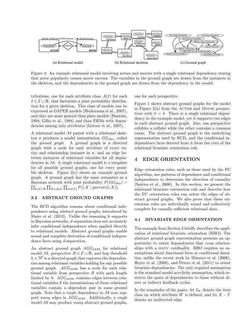
well as cardinality constraints for the number of en-tity instances involved in a relationship. A schema istypically depicted with an entity-relationship diagram,such as the one underlying the model shown in Fig-ure 2(a). This example has two entity classes—Actorwith attribute Popularity and Movie with attributeSuccess—and one relationship class—Stars-In withno attributes. The cardinality constraints (expressedas crow’s feet in the diagram) indicate that many ac-tors may appear in a movie and a single actor mayappear in many movies. A schema is a template for arelational skeleton σ—a data set of entity and relation-ship instances. The example in Figure 2(b) containsfour Actor instances, five Movie instances, and therelationships among them.
Given a relational schema, one can specify relationalpaths, which are critical for specifying the variablesand dependencies of a relational model. A relationalpath is an alternating sequence of entity and relation-ship classes that follow connected paths in the schema(subject to cardinality constraints). In Figure 2(a),possible relational paths include [Actor] (a singletonpath specifying an actor), [Movie, Stars-In, Actor](specifying the actors in a movie), or even [Actor,Stars-In, Movie, Stars-In, Actor] (describing co-stars). The cardinality of a relational path is many ifthe cardinalities along the path indicate that it couldreach more than one instance; otherwise, the cardi-nality is one. For example, card([Movie, Stars-In,Actor]) = many since a movie can reach many ac-tors, whereas card([Actor]) = one since this pathcan only reach the base actor instance.
Relational variables consist of a relational path andan attribute, and they describe attributes of classesreached via a relational path (e.g., the popularity of ac-tors starring in a movie). Relational dependencies con-sist of a pair of relational variables with a common firstitem, called the perspective. The dependency in Fig-ure 2(a) states that the popularity of actors influencesthe success of movies they star in. A canonical depen-dency has a single item class in the relational path ofthe effect variable. A relational model, M = (S,D), isa collection of relational dependencies D, in canonicalform, defined over schema S. Relational models areparameterized by a set of conditional probability dis-
GoodfellasSuccess
STARS-IN
STARS-IN
Tom Hanks
Popularity Joe Pesci
Popularity
Apollo 13Success
STAR
S-IN
Gary Sinise
PopularityForrest GumpSuccess
STARS-IN
STAR
S-IN
Sharon Stone
Popularity
CasinoSuccessThe Quick and
the Dead
Success
STARS-IN
STARS-IN STARS-IN
STARS-IN
Tom Hanks.Popularity Joe Pesci.Popularity
Gary Sinise.Popularity
Sharon Stone.Popularity
Forrest Gump.Success
Apollo 13.SuccessThe Quick and the Dead.Success
Casino.Success
Goodfellas.Success
(a) Relational model (b) Relational skeleton (c) Ground graph
STARS-IN
MOVIEACTOR
[MOVIE, STARS-IN, ACTOR].Popularity [MOVIE].Success
Popularity Success
Figure 2: An example relational model involving actors and movies with a single relational dependency statingthat actor popularity causes movie success. The variables in the ground graph are drawn from the instances inthe skeleton, and the dependencies in the ground graph are drawn from the dependency in the model.
tributions, one for each attribute class A(I) for eachI ∈ E ∪R, that factorizes a joint probability distribu-tion for a given skeleton. This class of models can beexpressed as DAPER models (Heckerman et al., 2007),and they are more general than plate models (Buntine,1994; Gilks et al., 1994) and than PRMs with depen-dencies among only attributes (Getoor et al., 2007).
A relational model M paired with a relational skele-ton σ produces a model instantiation GGMσ, calledthe ground graph. A ground graph is a directedgraph with a node for each attribute of every en-tity and relationship instance in σ, and an edge be-tween instances of relational variables for all depen-dencies in M. A single relational model is a templatefor all possible ground graphs, one for every possi-ble skeleton. Figure 2(c) shows an example groundgraph. A ground graph has the same semantics as aBayesian network with joint probability P (GGMσ) =�
I∈E∪R�
X∈A(I)
�i∈σ(I) P (i.X | parents(i.X)).
3.2 ABSTRACT GROUND GRAPHS
The RCD algorithm reasons about conditional inde-pendence using abstract ground graphs, introduced byMaier et al. (2013). Unlike the reasoning it supportsin Bayesian networks, d -separation does not accuratelyinfer conditional independence when applied directlyto relational models. Abstract ground graphs enablesound and complete derivation of conditional indepen-dence facts using d -separation.
An abstract ground graph AGGMBh for relationalmodel M, perspective B ∈ E ∪R, and hop thresholdh ∈ N0 is a directed graph that captures the dependen-cies among relational variables holding for any possibleground graph. AGGMBh has a node for each rela-tional variable from perspective B with path lengthlimited by h. AGGMBh contains edges between rela-tional variables if the instantiations of those relationalvariables contain a dependent pair in some groundgraph. Note that a single dependency in M may sup-port many edges in AGGMBh . Additionally, a singlemodel M may produce many abstract ground graphs,
one for each perspective.
Figure 1 shows abstract ground graphs for the modelin Figure 2(a) from the Actor and Movie perspec-tives with h = 4. There is a single relational depen-dency in the example model, yet it supports two edgesin each abstract ground graph. Also, one perspectiveexhibits a collider while the other contains a commoncause. The abstract ground graph is the underlyingrepresentation used by RCD, and the conditional in-dependence facts derived from it form the crux of therelational bivariate orientation rule.
4 EDGE ORIENTATION
Edge orientation rules, such as those used by the PCalgorithm, use patterns of dependence and conditionalindependence to determine the direction of causality(Spirtes et al., 2000). In this section, we present therelational bivariate orientation rule and describe howthe PC orientation rules can orient the edges of ab-stract ground graphs. We also prove that these ori-entation rules are individually sound and collectivelycomplete for causally sufficient relational data.
4.1 BIVARIATE EDGE ORIENTATION
The example from Section 2 briefly describes the appli-cation of relational bivariate orientation (RBO). Theabstract ground graph representation presents an op-portunity to orient dependencies that cross relation-ships with a many cardinality. RBO requires no as-sumptions about functional form or conditional densi-ties, unlike the recent work by Shimizu et al. (2006),Hoyer et al. (2008), and Peters et al. (2011) to orientbivariate dependencies. The only required assumptionis the standard model acyclicity assumption, which re-stricts the space of dependencies to those without di-rect or indirect feedback cycles.
In the remainder of the paper, let IW denote the itemclass on which attribute W is defined, and let X − Ydenote an undirected edge.
[IX ... IY ].Y ∈ sepset([IX ].X, [IX ... IY ... IX ].X)?
[IX ... IY ].Y
[IX ].X [IX ... IY ... IX ].X
NO
YES [IX ... IY ].Y
[IX ].X [IX ... IY ... IX ].X
[IX ... IY ].Y
[IX ].X [IX ... IY ... IX ].X
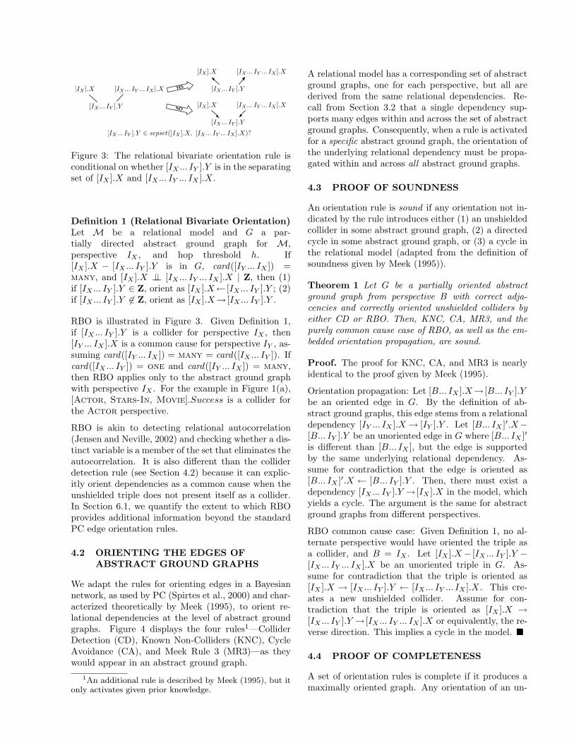
Figure 3: The relational bivariate orientation rule isconditional on whether [IX ... IY ].Y is in the separatingset of [IX ].X and [IX ... IY ... IX ].X.
Definition 1 (Relational Bivariate Orientation)Let M be a relational model and G a par-tially directed abstract ground graph for M,perspective IX , and hop threshold h. If[IX ].X − [IX ... IY ].Y is in G, card([IY ... IX ]) =many, and [IX ].X ⊥⊥ [IX ... IY ... IX ].X | Z, then (1)if [IX ... IY ].Y ∈ Z, orient as [IX ].X← [IX ... IY ].Y ; (2)if [IX ... IY ].Y �∈ Z, orient as [IX ].X→ [IX ... IY ].Y .
RBO is illustrated in Figure 3. Given Definition 1,if [IX ... IY ].Y is a collider for perspective IX , then[IY ... IX ].X is a common cause for perspective IY , as-suming card([IY ... IX ]) = many = card([IX ... IY ]). Ifcard([IX ... IY ]) = one and card([IY ... IX ]) = many,then RBO applies only to the abstract ground graphwith perspective IX . For the example in Figure 1(a),[Actor, Stars-In, Movie].Success is a collider forthe Actor perspective.
RBO is akin to detecting relational autocorrelation(Jensen and Neville, 2002) and checking whether a dis-tinct variable is a member of the set that eliminates theautocorrelation. It is also different than the colliderdetection rule (see Section 4.2) because it can explic-itly orient dependencies as a common cause when theunshielded triple does not present itself as a collider.In Section 6.1, we quantify the extent to which RBOprovides additional information beyond the standardPC edge orientation rules.
4.2 ORIENTING THE EDGES OFABSTRACT GROUND GRAPHS
We adapt the rules for orienting edges in a Bayesiannetwork, as used by PC (Spirtes et al., 2000) and char-acterized theoretically by Meek (1995), to orient re-lational dependencies at the level of abstract groundgraphs. Figure 4 displays the four rules1—ColliderDetection (CD), Known Non-Colliders (KNC), CycleAvoidance (CA), and Meek Rule 3 (MR3)—as theywould appear in an abstract ground graph.
1An additional rule is described by Meek (1995), but itonly activates given prior knowledge.
A relational model has a corresponding set of abstractground graphs, one for each perspective, but all arederived from the same relational dependencies. Re-call from Section 3.2 that a single dependency sup-ports many edges within and across the set of abstractground graphs. Consequently, when a rule is activatedfor a specific abstract ground graph, the orientation ofthe underlying relational dependency must be propa-gated within and across all abstract ground graphs.
4.3 PROOF OF SOUNDNESS
An orientation rule is sound if any orientation not in-dicated by the rule introduces either (1) an unshieldedcollider in some abstract ground graph, (2) a directedcycle in some abstract ground graph, or (3) a cycle inthe relational model (adapted from the definition ofsoundness given by Meek (1995)).
Theorem 1 Let G be a partially oriented abstractground graph from perspective B with correct adja-cencies and correctly oriented unshielded colliders byeither CD or RBO. Then, KNC, CA, MR3, and thepurely common cause case of RBO, as well as the em-bedded orientation propagation, are sound.
Proof. The proof for KNC, CA, and MR3 is nearlyidentical to the proof given by Meek (1995).
Orientation propagation: Let [B... IX ].X→ [B... IY ].Ybe an oriented edge in G. By the definition of ab-stract ground graphs, this edge stems from a relationaldependency [IY ... IX ].X → [IY ].Y . Let [B... IX ]�.X−[B... IY ].Y be an unoriented edge in G where [B... IX ]�is different than [B... IX ], but the edge is supportedby the same underlying relational dependency. As-sume for contradiction that the edge is oriented as[B... IX ]�.X ← [B... IY ].Y . Then, there must exist adependency [IX ... IY ].Y → [IX ].X in the model, whichyields a cycle. The argument is the same for abstractground graphs from different perspectives.
RBO common cause case: Given Definition 1, no al-ternate perspective would have oriented the triple asa collider, and B = IX . Let [IX ].X− [IX ... IY ].Y −[IX ... IY ... IX ].X be an unoriented triple in G. As-sume for contradiction that the triple is oriented as[IX ].X → [IX ... IY ].Y ← [IX ... IY ... IX ].X. This cre-ates a new unshielded collider. Assume for con-tradiction that the triple is oriented as [IX ].X →[IX ... IY ].Y → [IX ... IY ... IX ].X or equivalently, the re-verse direction. This implies a cycle in the model. �
4.4 PROOF OF COMPLETENESS
A set of orientation rules is complete if it produces amaximally oriented graph. Any orientation of an un-

[B... IX ].X
[B... IY ].Y
[B... IZ ].Z
[B... IW ].W
[B... IX ].X
[B... IY ].Y
[B... IZ ].Z
[B... IW ].W
[B... IY ].Y
[B... IX ].X [B... IZ ].Z
[B... IY ].Y
[B... IX ].X [B... IZ ].Z
[B... IY ].Y �∈ sepset([B... IX ].X, [B... IZ ].Z)
[B... IY ].Y
[B... IX ].X [B... IZ ].Z
[B... IY ].Y
[B... IX ].X [B... IZ ].Z
(a) Collider Detection (CD) (b) Known Non-Colliders (KNC)
(c) Cycle Avoidance (CA) (d) Meek Rule 3 (MR3)
[B... IY ].Y
[B... IX ].X [B... IZ ].Z
[B... IY ].Y
[B... IX ].X [B... IZ ].Z
Figure 4: Schematics of the PC orientation rules on an abstract ground graph from perspective B.
oriented edge must be consistent with a member of theMarkov equivalence class. Lemma 1 describes a use-ful property that enables the proof of completeness toreason directly about the remaining unoriented edges.
Lemma 1 Let G be a partially oriented abstractground graph, with correct adjacencies and orientedunshielded colliders. Let Go be the result of exhaus-tively applying KNC, CA, MR3, and the purely com-mon cause case of RBO all with orientation propaga-tion. In Go, if P.X→P �.Y−P ��.Z, then P.X→P ��.Z.
Proof. Much of this proof follows from Meek (1995).
The following properties hold: (1) X �= Z; otherwise,RBO would have oriented P �.Y ←P ��.Z. (2) P.X mustbe adjacent to P ��Z; otherwise, KNC would have ori-ented P �.Y → P ��.Z. (3) P.X ← P ��.Z does not hold;otherwise, CA would have oriented P �.Y ← P ��.Z.Therefore, we have a structure of the form P.X →P �.Y −P ��.Z and P.X−P ��.Z.
We show that P.X → P ��.Z through exhaustive enu-meration of the cases under which P.X → P �.Y wasoriented. The cases for KNC, CD (and RBO collidercases), CA, and MR3 follow directly from Meek (1995).
(1) RBO oriented P.X → P �.Y from the IY per-spective as a common cause. Then, P � = [IY ],P = [IY ... IX ], and P �� = [IY ... IZ ]. Also,[IY ... IX ... IY ].Y must be in Go with [IY ... IX ].X →[IY ... IX ... IY ].Y . By Definition 1, card([IY ... IX ]) =one and card([IY ... IX ])=many.
The relational path [IY ... IZ ] and its reverse have car-dinality one; otherwise, RBO would have oriented[IY ].Y − [IY ... IZ ].Z. We show that [IY ... IX ].X −[IY ... IZ ].Z cannot remain unoriented.
Since this edge exists, by the construction of abstractground graphs, (a) [IY ... IX ] must be produced bycombining [IY ... IZ ] and [IZ ... IX ]) (using the extendmethod (Maier et al., 2013)) and (b) [IY ... IZ ] mustbe produced by combining [IY ... IX ] and [IX ... IZ ]).The paths [IX ... IZ ] and [IZ ... IX ] underlie the depen-
dency between X and Z. Facts (a) and (b) imposeconstraints on the schema and abstract ground graphs.There are four cases for (a) depending on the relation-ship between [IY ... IZ ] and [IZ ... IX ], with equivalentcases for (b).
(i) [IY ... IZ ] and [IZ ... IX ] overlap exactly at IZ .Then, the path from IX to IZ must have car-dinality many. This implies that from the IZ
perspective, RBO would have oriented X to Z.(ii) [IY ... IM ... IZ ] and [IZ ... IM ... IX ] overlap up to
IM . This is equivalent to case (i), except IM
appears on the path from IX to IZ .(iii) [IZ ... IX ] is a subpath of the reverse of [IY ... IZ ].
Then, the path from IZ to IY must have cardi-nality many, which is a contradiction.
(iv) The reverse of [IY ... IZ ] is a subpath of [IZ ... IX ].This is equivalent to case (i), except IY appearson the path from IX to IZ .
(2) Orientation propagation oriented P.X → P �.Y .Then, there exists an edge for some perspective thatwas oriented by one of the orientation rules. From thatperspective, the local structure matches the given pat-tern, and from the previous cases, X→Z was oriented.By definition, P.X→P ��.Z. �
Meek (1995) also provides the following results, usedfor proving completeness. A chordal graph is an undi-rected graph where every undirected cycle of lengthfour or more has an edge between two nonconsecutivevertices on the cycle. Let G be an undirected graph, αa total order on the vertices of G, and Gα the induceddirected graph (A→B is in Gα if and only if A < Bwith respect to α). A total order α is consistent withrespect to G if and only if Gα has no unshielded col-liders. It can be shown that only chordal graphs haveconsistent orderings. Finally, if G is an undirectedchordal graph, then for all pairs of adjacent verticesA and B in G, there exist consistent total orderings αand γ such that A→B in Gα and A←B in Gγ .
Theorem 2 Given a partially oriented abstractground graph, with correct adjacencies and oriented

unshielded colliders, exhaustively applying KNC, CA,MR3, and RBO all with orientation propagation re-sults in a maximally oriented graph G.
Proof. Much of this proof follows from Meek (1995).Let Eu and Eo be the set of unoriented edges andoriented edges of G, respectively.Claim 1: No orientation of edges in Eu creates a cycleor unshielded collider in G that includes edges from Eo.Proof. Assume there exists an orientation of edges inEu that creates a cycle using edges from Eo. Withoutloss of generality, assume that the cycle is of lengththree. (1) If A→B→C are in Eo and A−C in Eu,then CA would have oriented A→C. (2) If A→B←Cor A←B→C are in Eo and A−C is in Eu, then noorientation A−C would create a cycle. (3) If A→B isin Eo and B−C−A in Eu, then by Lemma 1 we haveA→C and no orientation of B−C would create a cycle.A similar argument holds for unshielded colliders. �Claim 2: Let Gu be the subgraph of G containingonly unoriented edges. Gu is the union of disjointchordal graphs.Proof. Assume that Gu is not the union of disjointchordal graphs. Then, there exists at least one disjointcomponent of Gu that is not a chordal graph. Recallthat no total ordering of Gu is consistent. Let A→B←C be an unshielded collider induced by some orderingon Gu. There are two cases: (1) A and C are adjacentin G. The edge must be oriented; otherwise, it wouldappear in Gu. Both orientations of A−C imply anorientation of A and B, or C and B, by Lemma 1.(2) A and C are not adjacent in G. Then, A−B−C isan unshielded triple in G. Either CD or RBO wouldhave oriented the triple as a collider, or the triple isinconsistent with the total ordering on Gu. �Since G is chordal, it follows that no orientation ofthe unoriented edges in G creates a new unshieldedcollider or cycle. �
5 The RCD Algorithm
The relational causal discovery (RCD) algorithm isa sound and complete constraint-based algorithm forlearning causal models from relational data.2 RCDemploys a similar strategy to the PC algorithm, op-erating in two distinct phases (Spirtes et al., 2000).RCD is similar to the Relational PC (RPC) algorithm,which also learns causal relational models (Maier et al.,2010). The differences between RPC and RCD arethreefold: (1) The underlying representation for RCDis a set of abstract ground graphs; (2) RCD employs anew causal constraint—the relational bivariate orien-tation rule; and (3) RCD is sound and complete. RPCalso reasons about the uncertainty of relationship ex-istence, but RCD assumes a prior relational skeleton.
ALGORITHM 1: RCD(schema, depth, hopThreshold , P )
1 PDs ← getPotentialDeps(schema, hopThreshold)2 N ← initializeNeighbors(schema, hopThreshold)3 S ← {}
// Phase I
4 for d← 0 to depth do5 for X → Y ∈ PDs do6 foreach condSet ∈ powerset(N [Y ] \ {X})
do7 if |condSet | = d then8 if X ⊥⊥ Y | condSet in P then9 PDs ← PDs \ {X → Y, Y → X}
10 S[X, Y ]← condSet11 break
// Phase II
12 AGGs ← buildAbstractGroundGraph(PDs)13 AGGs, S ← ColliderDetection(AGGs, S)14 AGGs, S ← BivariateOrientation(AGGs, S)15 while changed do16 AGGs ← KnownNonColliders(AGGs, S)17 AGGs ← CycleAvoidance(AGGs, S)18 AGGs ← MeekRule3(AGGs, S)19 return getCanonicalDependencies(AGGs)
The remainder of this section describes the algorithmicdetails of RCD and proves its correctness.
Algorithm 1 provides pseudocode for RCD. Initially,RCD enumerates the set of potential dependencies, incanonical form, with relational paths limited by thehop threshold (line 1). Phase I continues similarly toPC, removing potential dependencies via conditionalindependence tests with conditioning sets of increasingsize drawn from the power set of neighbors of the effectvariable (lines 4–11). Every identified separating set isrecorded, and the corresponding potential dependencyand its reverse are removed (lines 9–10).
The second phase of RCD determines the orientationof dependencies consistent with the conditional inde-pendencies discovered in Phase I. First, Phase II con-structs a set of undirected abstract ground graphs, onefor each perspective, given the remaining dependen-cies. RCD then iteratively checks all edge orientationrules, as described in Section 4. Phase II of RCD isalso different from PC and RPC because it searches foradditional separating sets while finding colliders andcommon causes with CD and RBO. Frequently, un-shielded triples X−Y −Z may have no separating setrecorded for X and Z. For these pairs, RCD attemptsto discover a new separating set, as in Phase I. Thesetriples occur for one of three reasons: (1) Since X andZ are relational variables, the separating set may havebeen discovered from an alternative perspective; (2)The total number of hops in the relational paths forX, Y , and Z may exceed the hop threshold—each de-pendency is subject to the hop threshold, but a pair of
2Code available at kdl.cs.umass.edu/rcd.

dependencies is limited by twice the hop threshold; or(3) The attributes of relational variables X and Z arethe same, which is necessarily excluded as a potentialdependency by the assumption of an acyclic model.
Given the algorithm description and the soundness andcompleteness of the edge orientation rules, we provethat RCD is sound and complete. The proof assumescausal sufficiency and a prior relational skeleton (i.e.,no causes of the relational structure).
Theorem 3 Given a schema and probability distri-bution P , RCD learns a correct maximally orientedmodel M assuming perfect conditional independencetests, sufficient hop threshold h, and sufficient depth.
Proof sketch. Given sufficient h, the set of poten-tial dependencies PDs includes all true dependenciesin M, and the set of neighbors N includes the truecauses for every effect relational variable. Assumingperfect conditional independence tests, PDs includesexactly the undirected true dependencies after Phase I,and S[X,Y ] records a correct separating set for the re-lational variable pair �X,Y �. However, there may existnon-adjacent pairs of variables that have no recordedseparating set (for the three reasons mentioned above).Given the remaining dependencies in PDs, we con-struct the correct set of edges in AGGs using the meth-ods from Maier et al. (2013). Next, all unshieldedcolliders are oriented by either CD or RBO, with cor-rectness following from Spirtes et al. (2000) and rela-tional d -separation (Maier et al., 2013). Whenever apair �X,Y � is missing a separating set in S, it is eitherfound as in Phase I or from a different perspective.RCD then produces a maximally oriented model bythe soundness (Theorem 1) and completeness (Theo-rem 2) results of the remaining orientation rules. �
6 EXPERIMENTS
6.1 SYNTHETIC EXPERIMENTS
The proofs of soundness and completeness offer aqualitative measure of RCD’s effectiveness—no othermethod can learn a more accurate causal model fromobservational data. To complement the theoretical re-sults, we provide a quantitative measure of RCD’s per-formance and compare against the performance of al-ternative constraint-based algorithms.
We evaluate RCD against two alternative algorithms.The first algorithm is RPC (Maier et al., 2010). Thisprovides a comparison against current state-of-the-artrelational learning. The second algorithm is the PCalgorithm executed on relational data that has beenpropositionalized from a specific perspective—termedPropositionalized PC (PPC). Propositionalization re-
duces relational data to a single, propositional table(Kramer et al., 2001). We take the best and worstperspectives for each trial by computing the averageF-score of its skeleton and compelled models.
We generated 1,000 random causal models over ran-domly generated schemas for each of the followingcombinations: entities (1–4); relationships (one lessthan the number of entities) with cardinalities selecteduniformly at random; attributes per item drawn fromPois(λ = 1)+1; and relational dependencies (1–15)limited by a hop threshold of 4 and at most 3 par-ents per variable. This procedure yielded a total of60,000 synthetic models. Note that this generates sim-ple Bayesian networks when there is a single entityclass. We ran RCD, RPC, and PPC for each perspec-tive, using a relational d -separation oracle with hopthreshold 8 for the abstract ground graphs.
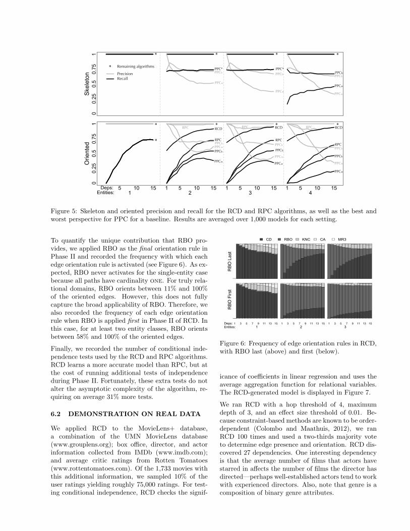
We compare the learned causal models with the truecausal model. For each trial, we record the precision(the proportion of learned edges in the true model)and recall (the proportion of true edges in the learnedmodel) for both the undirected skeleton after Phase Iand the partially orientated model after Phase II. Fig-ure 5 displays the average across 1,000 trials for eachalgorithm and measure. We omit error bars as themaximum standard error was less than 0.015.
All algorithms learn identical models for the single-entity case because they reduce to PC when analyz-ing propositional data. For truly relational data, algo-rithms that reason over relational representations arenecessary for accurate learning. RCD and RPC re-cover the exact skeleton, whereas the best and worstPPC cases learn flawed skeletons (and also flawed ori-ented models), with high false positive and high falsenegative rates. This is evidence that propositionaliz-ing relational data may lead to inaccurately learnedcausal models.
For oriented models, the RCD algorithm vastly ex-ceeds the performance of all other algorithms. Asthe soundness result suggests, RCD achieves a com-pelled precision of 1.0, whereas RPC introduces ori-entation errors due to reasoning over the class depen-dency graph and missing additional separating sets.For recall, which is closely tied to the completeness re-sult, RCD ranges from roughly 0.56 (for 1 dependencyand 2 entities) to 0.94 (for 15 dependencies and 4 enti-ties). While RPC and PPC cannot orient models witha single dependency, the relational bivariate orienta-tion rule enables RCD to orient models using little in-formation. RCD also discovers more of the underlyingcausal structure as the complexity of the domain in-creases, with respect to both relational structure (moreentity and relationship classes) and model density.
00.25
0.5
0.75
1Skeleton
5 10 15 1 5 10 15 1 5 10 15 1 5 10 151 2 3 4
Deps:Entities:
00.25
0.5
0.75
1Oriented
* * * *
****
PPC*PPCb
PPCw
PPCb
PPCw
PPC*PPCbPPCb
PPCw
PPCw
* RPC RPCRPC
RPCRPCRPC RCDRCDRCD
PPCbPPCbPPCb
PPCwPPCw
PPCw
* Remaining algorithms
PrecisionRecall
PPCbPPCw
PPCw
PPCw
PPCb
PPCb
Figure 5: Skeleton and oriented precision and recall for the RCD and RPC algorithms, as well as the best andworst perspective for PPC for a baseline. Results are averaged over 1,000 models for each setting.
To quantify the unique contribution that RBO pro-vides, we applied RBO as the final orientation rule inPhase II and recorded the frequency with which eachedge orientation rule is activated (see Figure 6). As ex-pected, RBO never activates for the single-entity casebecause all paths have cardinality one. For truly rela-tional domains, RBO orients between 11% and 100%of the oriented edges. However, this does not fullycapture the broad applicability of RBO. Therefore, wealso recorded the frequency of each edge orientationrule when RBO is applied first in Phase II of RCD. Inthis case, for at least two entity classes, RBO orientsbetween 58% and 100% of the oriented edges.
Finally, we recorded the number of conditional inde-pendence tests used by the RCD and RPC algorithms.RCD learns a more accurate model than RPC, but atthe cost of running additional tests of independenceduring Phase II. Fortunately, these extra tests do notalter the asymptotic complexity of the algorithm, re-quiring on average 31% more tests.
6.2 DEMONSTRATION ON REAL DATA
We applied RCD to the MovieLens+ database,a combination of the UMN MovieLens database(www.grouplens.org); box office, director, and actorinformation collected from IMDb (www.imdb.com);and average critic ratings from Rotten Tomatoes(www.rottentomatoes.com). Of the 1,733 movies withthis additional information, we sampled 10% of theuser ratings yielding roughly 75,000 ratings. For test-ing conditional independence, RCD checks the signif-
Deps:Entities:
RBO
Las
tRB
O F
irst
CD RBO KNC CA MR3
1 3 5 7 9 11 13 15 1 3 5 7 9 11 13 15 1 3 5 7 9 11 13 151 2 3
Figure 6: Frequency of edge orientation rules in RCD,with RBO last (above) and first (below).
icance of coefficients in linear regression and uses theaverage aggregation function for relational variables.The RCD-generated model is displayed in Figure 7.
We ran RCD with a hop threshold of 4, maximumdepth of 3, and an effect size threshold of 0.01. Be-cause constraint-based methods are known to be order-dependent (Colombo and Maathuis, 2012), we ranRCD 100 times and used a two-thirds majority voteto determine edge presence and orientation. RCD dis-covered 27 dependencies. One interesting dependencyis that the average number of films that actors havestarred in affects the number of films the director hasdirected—perhaps well-established actors tend to workwith experienced directors. Also, note that genre is acomposition of binary genre attributes.

ACTOR
Gender
DIRECTOR
Gender
MOVIEBudget
Critic Rating Gross
Genre
Actor Count
Rating Count
RATES
Rating
USER
Gender Age
Movie Count
Age
STARS-INMovie Count
Age
DIRECTS
Rating CountRuntime
Rank
Figure 7: RCD-learned model of MovieLens+.
7 RELATED WORK
The ideas presented in this paper are related to threeprimary areas of research. First, the RCD algorithmis a constraint-based method for learning causal struc-ture from observed conditional independencies. Thevast majority of other causal discovery algorithms havefocused on Bayesian networks and propositional data.The IC (Pearl, 2000) and PC (Spirtes et al., 2000) algo-rithms provided a foundation for all future constraint-based methods, and Meek (1995) proved these equiv-alent methods to be sound and complete for causallysufficient data. Additional constraint-based methodsinclude the Grow-Shrink (Margaritis and Thrun, 1999)and TC (Pellet and Elisseeff, 2008) algorithms.
Second, RCD emphasizes learning causal relationalmodels, a more expressive class of models for real-world systems. Our experimental results also indicatethat propositional approaches may be inadequate tohandle the additional complexity of relational data.Algorithms for learning the structure of directed rela-tional models have been limited to methods based onsearch-and-score that do not identify Markov equiva-lence classes (Friedman et al., 1999). The RPC algo-rithm was the first to employ constraint-based meth-ods to learn causal models from relational data (Maieret al., 2010), but RPC is not complete and may intro-duce errors due to its underlying representation. BothRPC and PRMs include capabilities to reason aboutrelationship existence (Getoor et al., 2002); however,we currently focus on attributional dependencies andleave causes of existence as future work.
Finally, orienting bivariate dependencies, the most ef-fective constraint used by RCD, is similar to the effortsof Shimizu et al. (2006), Hoyer et al. (2008), and Peterset al. (2011) in the propositional setting. Contrary toRBO, these techniques leverage strong assumptions onfunctional form and asymmetries in conditional densi-ties to determine the direction of causality. Nonethe-less, these methods could orient some of the edges that
remain unoriented by RCD, given these additional dis-tributional assumptions.
8 CONCLUSIONS
Relational d -separation and the abstract ground graphrepresentation provide a new opportunity to developtheoretically correct algorithms for learning causalstructure from relational data. We presented the re-lational causal discovery (RCD) algorithm and provedit sound and complete for discovering causal modelsfrom causally sufficient relational data. We introducedrelational bivariate orientation (RBO), which can de-tect the orientation of bivariate dependencies. Thisleads to recall of oriented relational models over a pre-vious state-of-the-art algorithm that is 18% to 72%greater on average. We also demonstrated RCD’s ef-fectiveness on synthetic causal relational models anddemonstrated its applicability to real-world data.
There are several clear avenues for future research.RCD could be extended to reason about entity and re-lationship existence, and the assumptions of causal suf-ficiency and acyclic models could be relaxed to supportreasoning about latent common causes and temporaldynamics. There are also new operators that exploitrelational structure, such as relational blocking (Ratti-gan et al., 2011), which could be integrated with sim-ple tests of conditional independence. Finally, RCDcould be enhanced with Bayesian information, similarto the recent work by Claassen and Heskes (2012) forimproving the reliability of algorithms that learn thestructure of Bayesian networks.
Acknowledgments
The authors wish to thank Cindy Loiselle for her edit-ing expertise. This effort is supported by the Intel-ligence Advanced Research Project Agency (IARPA)via Department of Interior National Business Cen-ter Contract number D11PC20152, Air Force Re-search Lab under agreement number FA8750-09-2-0187, the National Science Foundation under grantnumber 0964094, and Science Applications Interna-tional Corporation (SAIC) and DARPA under con-tract number P010089628. The U.S. Government isauthorized to reproduce and distribute reprints forgovernmental purposes notwithstanding any copyrightnotation hereon. The views and conclusions containedherein are those of the authors and should not be in-terpreted as necessarily representing the official poli-cies or endorsements either expressed or implied, ofIARPA, DoI/NBC, AFRL, NSF, SAIC, DARPA or theU.S. Government. The Greek State Scholarships Foun-dation partially supported Katerina Marazopoulou.

References
W. L. Buntine. Operations for learning with graphicalmodels. Journal of Artificial Intelligence Research,2:159–225, 1994.
T. Claassen and T. Heskes. A Bayesian approach toconstraint based causal inference. In Proceedingsof the Twenty-Eighth Annual Conference on Uncer-tainty in Artificial Intelligence, pages 207–216, 2012.
D. Colombo and M. H. Maathuis. A Modificationof the PC Algorithm Yielding Order-IndependentSkeletons. arXiv preprint arXiv:1211.3295, 2012.
N. Friedman, L. Getoor, D. Koller, and A. Pfeffer.Learning probabilistic relational models. In Inter-national Joint Conference on Artificial Intelligence,volume 16, pages 1300–1309, 1999.
L. Getoor, N. Friedman, D. Koller, and B. Taskar.Learning probabilistic models of link structure.Journal of Machine Learning Research, 3:679–707,2002.
L. Getoor, N. Friedman, D. Koller, A. Pfeffer, andB. Taskar. Probabilistic relational models. InL. Getoor and B. Taskar, editors, Introduction toStatistical Relational Learning, pages 129–174. MITPress, Cambridge, MA, 2007.
W. R. Gilks, A. Thomas, and D. J. Spiegelhalter. Alanguage and program for complex Bayesian model-ing. The Statistician, 43:169–177, 1994.
D. Heckerman, C. Meek, and D. Koller. Probabilisticentity-relationship models, PRMs, and plate mod-els. In L. Getoor and B. Taskar, editors, Introduc-tion to Statistical Relational Learning, pages 201–238. MIT Press, Cambridge, MA, 2007.
P. O. Hoyer, D. Janzing, J. M. Mooij, J. Peters, andB. Scholkopf. Nonlinear causal discovery with addi-tive noise models. In Advances in Neural Informa-tion Processing Systems 22, pages 689–696, 2008.
D. Jensen and J. Neville. Linkage and autocorrelationcause feature selection bias in relational learning. InProceedings of the Nineteenth International Confer-ence on Machine Learning, pages 259–266, 2002.
S. Kramer, N. Lavrac, and P. Flach. Propositional-ization approaches to relational data mining. InS. Dzeroski and N. Lavrac, editors, Relational DataMining, pages 262–286. Springer-Verlag, New York,NY, 2001.
M. Maier, B. Taylor, H. Oktay, and D. Jensen. Learn-ing causal models of relational domains. In Pro-ceedings of the Twenty-Fourth AAAI Conference onArtificial Intelligence, pages 531–538, 2010.
M. Maier, K. Marazopoulou, and D. Jensen. Reason-ing about Independence in Probabilistic Models ofRelational Data. arXiv preprint arXiv:1302.4381,
2013.D. Margaritis and S. Thrun. Bayesian network induc-
tion via local neighborhoods. In Advances in NeuralInformation Processing Systems 12, pages 505–511,1999.
C. Meek. Causal inference and causal explanationwith background knowledge. In Proceedings of theEleventh Conference on Uncertainty in Artificial In-telligence, pages 403–410, 1995.
J. Pearl. Causality: Models, Reasoning, and Inference.Cambridge University Press, New York, NY, 2000.
J.-P. Pellet and A. Elisseeff. Using Markov blanketsfor causal structure learning. Journal of MachineLearning Research, 9:1295–1342, 2008.
J. Peters, D. Janzing, and B. Scholkopf. Causal in-ference on discrete data using additive noise mod-els. IEEE Transactions on Pattern Analysis andMachine Intelligence, 33(12):2436–2450, 2011.
M. J. Rattigan, M. Maier, and D. Jensen. Relationalblocking for causal discovery. In Proceedings of theTwenty-Fifth AAAI Conference on Artificial Intel-ligence, pages 145–151, 2011.
S. Shimizu, P. O. Hoyer, A. Hyvarinen, and A. Kermi-nen. A linear non-gaussian acyclic model for causaldiscovery. Journal of Machine Learning Research,7:2003–2030, 2006.
P. Spirtes, C. Glymour, and R. Scheines. Causation,Prediction and Search. MIT Press, Cambridge, MA,2nd edition, 2000.