a socio-public health data-based introductory statistics...
TRANSCRIPT

A socio-public health data-based introductory statistics course
Murray Aitkin
School of Mathematics and Statistics
The University of Melbourne
Australia
– p. 1

Turbulence in the profession!
• A widespread dissatisfaction with the present curriculum.• p-values banned by a minor psychology journal.• ASA statement on p-values recommending their
replacement – but by what?• Q-step support by ESRC and the Nuffield Foundation of the
development of new statistics or “quantitative methods"courses for social science graduate and undergraduatestudents by the social science departments themselves,without the participation of statistics departments.
• Statistics departments sidelined? A warning bell ringing!• Special issue (November 2015) of The American
Statistician on statistics and the undergraduate curriculum.• The Statistical Society of Australia held a two-day workshop
(June 2016) to develop proposals for modernising statisticscourses at all levels of school and University.
– p. 2

Do we need a new introductory stat course?
The editors of the TAS special issue focussed on second- andhigher-level courses:
Likely the first and most important place to start thecurriculum conversation is with the courses that followan introductory statistics course. (N.J. Horton and J.S.Hardin, Special issue editors)
George Cobb, Mount Holyoke College, did not agree with that:
Mere renovation is too little too late: we need to rethinkour undergraduate curriculum from the ground up.
The Special Issue has a curious absence of discussion ofcontent for the first course, apart from issues like bootstrappingreplacing parametric inference.
The SSA subgroup which considered the undergraduatecurriculum came to a consensus on the first course: it should bedata-, models-, and probability-oriented.
– p. 3

Why do we need a new introductory course? – Cobb
... I have come to the conclusion that our consensus about curriculum needsto be rebuilt from the ground up. Our territory – thinking with and about data– is too valuable to allow old curricular structures to continue to sitcontentedly on their aging assets while more vigorous neighbours takeadvantage of our latest ideas. (p. 267)
... Markov chain Monte Carlo and related methods have led to a widespreaduse of Bayesian methods for applied work, which use, in turn, has led to amajor reversal of an earlier prejudice against what had long been dismissedas an inappropriately subjective approach to data analysis. (p.270)
... If we are truly to rethink our curriculum at a deep level, we ought to startwith foundations.
I am convinced we will need an extended period of ferment,experimentation, and settling out to reach a new consensus on content,much as it took us decades to reach the old consensus on the nowmiddle-aged introductory course. (p. 273)
– p. 4

What’s in the traditional intro stats course?
• Population and sample; descriptive statistics – mean andvariance – of a sample;
• simple probability; the normal distribution;• sampling distribution of the sample mean for the normal
distribution;• the Central Limit Theorem and the large-sample normal
distribution of the sample mean;• the z-test for a hypothetical mean with known variance;• the t-test for a hypothetical mean with unknown variance;• confidence intervals for the mean and for a population
proportion;• the t-test and confidence intervals for the difference of two
means and of two proportions;• simple linear regression and correlation.
– p. 5

What’s wrong with this? – what is missing?
• A data base. Students see small samples, and may have tocollect data themselves, but do not see a realistic largesurvey or small population data base.
• The research questions – why do we have these data? Whowants to know?
• The importance of the sample design – (not just forsampling distributions).
• An understanding of probability (though samplingdistributions are expected to be understood).
• The idea of a probability model.• Any principles for statistical inference (the Central Limit
Theorem is not an inferential principle).
– p. 6

An ancient syllabus
Apart from the t-test, this intro stat curriculum is pre-1900(Student’s use of the t-test was published in 1908).
How can all these extra topics be fitted into a course which isalready overstuffed?
They can’t, but space can be made by limiting the range ofmodels and analyses.
– p. 7

A successful non-standard course
• The data base – a small population of 1296 families in aChild Development Study at UC Berkeley.
• The research questions – what is the effect of mother’s (andfather’s) smoking on their child’s development through◦ birthweight;◦ physical and intellectual development at age 10.
• The study design.• Random sampling from the database.• The dangers of voluntary response and other non-random
sampling methods.• Sampling binary attributes: the binomial distribution.• Inference from sample to population: the likelihood function.
– p. 8

How to handle inference? – frequentist
Need the repeated-sampling distribution of the sampleproportion for confidence intervals (point estimates are of novalue, since they are always wrong).
Hand-waving needed (statistical theory shows that ...)
Confidence intervals for differences between proportions (morehand-waving) in 2x2 tables (No X2 test ...).
Continuous variables dichotomised at the median or commonmedian.
Not efficient but workable – same theory for differences.
Uncomfortable with hand-waving – Bayes is easier
– p. 9

How to handle inference? – Bayesian
Likelihood function conveys the data information.
How to turn this into a probability statement?
Prior distribution on p.
Finite population of size N , so p must be one of the values0/N, 1/N, ...,N/N .
If no prior preference for one of these over another, all haveequal prior probability 1/(N + 1).
Bayes’s theorem provides the solution.
How to demonstrate or justify it? – the screening test – a widelyused and useful example.
(New intro Bayesian book: Statistical Rethinking: a Bayesiancourse with examples in R and Stan. Richard McElreath,Chapman and Hall 2016.)
– p. 10

The screening test
• A condition C is uncommon – present in 2% of thepopulation.
• For those people who have the condition, the screening testgives a true positive result 95% of the time.
• For those people who do not have the condition, thescreening test gives a false positive result 10% of the time.
• We test a population of 1000 people in a small town. Thetrue positive and false positive rates apply to this townpopulation.
What do we conclude from the results of the screening test?
– p. 11

Venn diagram – contingency table
We write + if the test result is positive, and - if the test result isnegative.
We write yes if the person tested has the condition, and no if theperson tested does not have the condition.
The test results for the town are:
condition present
test yes no Total
+ 19 98 117- 1 882 883
Total 20 980 1000
What to conclude?
– p. 12

How effective is the screening test?
condition present
test yes no Total
+ 19 98 117- 1 882 883
Total 20 980 1000
• There are 20 (2%) cases and 980 (98%) non-cases.• Of the 20 cases, 19 (95%) are correctly identified – true +.• Of the 980 non-cases, 98 (10%) are incorrectly identified –
false +.• Of the 117 + tests, 19/117 (16%) are from people who had
the condition.• Of the 883 - tests, 1/883 (0.11%) are from people who had
the condition.– p. 13

Conclusion
• If your test was negative, you can be reasssured that youare very unlikely to have the condition.
• If your test was positive, the probability that you have thecondition is only 16%.
So what was the point of the screening test?
Many students find this shocking.
The true positive rate is 95%!
So surely almost everyone testing positive must have thecondition!
The fallacy of the transposed conditional.
Bayes’s theorem from a 2x2 table, without algebra.
– p. 14

The role of posterior simulation
• Bayesian analysis has been greatly enriched, but alsosimplified, by the ability to generate large numbers ofposterior draws of model parameters through MCMC,
• and to combine these in any way, with or without observeddata,
• to give posterior distributions of any functions of data andparameters.
This idea is new to students, and is illustrated here withsuccessively larger numbers of random draws from theBeta (4,8) distribution; we show the empirical cdf of the drawsand the true cdf (solid curve).
With 10,000 draws the empirical cdf is very smooth, andoverlaps the true cdf almost exactly.
– p. 15

Simulations from Beta(4,8)
0.0 0.2 0.4 0.6 0.8 1.0
0.0
0.1
0.2
0.3
0.4
0.5
0.6
0.7
0.8
0.9
1.0
p
cdf
(a) n = 10
0.0 0.2 0.4 0.6 0.8 1.0
0.0
0.1
0.2
0.3
0.4
0.5
0.6
0.7
0.8
0.9
1.0
p
cdf
(b) n=100
0.0 0.2 0.4 0.6 0.8 1.0
0.0
0.1
0.2
0.3
0.4
0.5
0.6
0.7
0.8
0.9
1.0
p
cdf
(c) n=1,000
0.0 0.2 0.4 0.6 0.8 1.0
0.0
0.1
0.2
0.3
0.4
0.5
0.6
0.7
0.8
0.9
1.0
p
cdf
(d) n=10,000
Figure 1: Empirical cdf (dots) of n draws from Beta(4,8), and– p. 16

RCT of Depepsen for the treatment of duodenal ulcers
Posterior simulations provide a simple procedure for credibleintervals for the difference in proportions responding in arandomised clinical trial:
– p. 17

RCT of Depepsen
• A study carried out at the Royal North Shore hospital inSydney by Professor D.W. Piper and co-workers.
• Depepsen (a trade name for sodium amylosulphate) hadbeen found effective in the treatment of gastric (stomach)ulcers.
• It was used in an RCT for duodenal ulcers, together withbest current treatment (bed rest, antacids, light diet,sedatives), and compared with placebo with current besttreatment.
• The criterion for success was complete healing of the ulcerwithin a period of 8 weeks after the beginning of treatment.
• 18 patients were randomised to Depepsen, and 17 toplacebo.
– p. 18
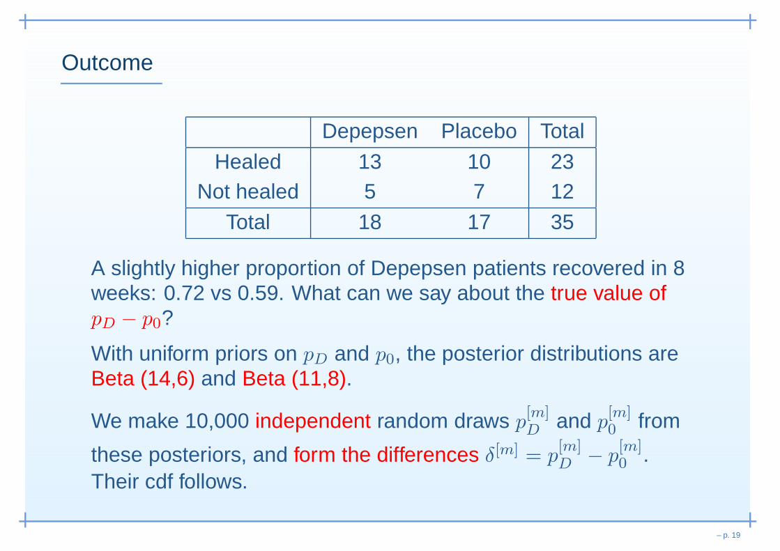
Outcome
Depepsen Placebo Total
Healed 13 10 23Not healed 5 7 12
Total 18 17 35
A slightly higher proportion of Depepsen patients recovered in 8weeks: 0.72 vs 0.59. What can we say about the true value ofpD − p0?
With uniform priors on pD and p0, the posterior distributions areBeta (14,6) and Beta (11,8).
We make 10,000 independent random draws p[m]D
and p[m]0 from
these posteriors, and form the differences δ[m] = p[m]D
− p[m]0 .
Their cdf follows.
– p. 19

Posterior densities placebo (dotted) and Depepsen
(solid)
0.0 0.2 0.4 0.6 0.8 1.0
0.0
0.5
1.0
1.5
2.0
2.5
3.0
3.5
p
Pro
babi
lity
dens
ity
– p. 20

Cdfs of 10,000 differences pD − p0
-0.4 -0.2 -0.0 0.2 0.4 0.6
0.0
0.1
0.2
0.3
0.4
0.5
0.6
0.7
0.8
0.9
1.0
Probability difference
cdf
– p. 21
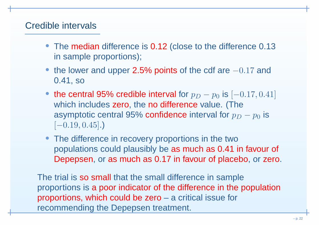
Credible intervals
• The median difference is 0.12 (close to the difference 0.13in sample proportions);
• the lower and upper 2.5% points of the cdf are −0.17 and0.41, so
• the central 95% credible interval for pD − p0 is [−0.17, 0.41]which includes zero, the no difference value. (Theasymptotic central 95% confidence interval for pD − p0 is[−0.19, 0.45].)
• The difference in recovery proportions in the twopopulations could plausibly be as much as 0.41 in favour ofDepepsen, or as much as 0.17 in favour of placebo, or zero.
The trial is so small that the small difference in sampleproportions is a poor indicator of the difference in the populationproportions, which could be zero – a critical issue forrecommending the Depepsen treatment.
– p. 22

Future treatments
Soon after this trial, a different drug treatment for duodenalulcers – cimetidine (trade name Tagamet) – was found to beeffective, and trials of Depepsen for the treatment of duodenalulcers were abandoned.
In the last ten years, these drug treatments, which were basedon reducing acidity in the stomach, have been replaced by anentirely different treatment with antibiotics –
It was discovered by Dr Barry J. Marshall and Dr J. RobinWarren of Perth, Western Australia, that most ulcers developfrom a stomach infection by the Helicobacter pylori bacterium,which responds rapidly to antibiotic drug treatment.
They were awarded the 2005 Nobel Prize for Medicine andPhysiology.
– p. 23

, Thank you! ,
– p. 24