A SLIDING MODE CONTROLLER FOR INDUCTION MOTOR DRIVES

A thesis submitted to National Institute of Technology, Rourkela,

for the award of the degree of

Master of Technology

In

ELECTRICAL ENGINEERING

(Power Control and Drives)

by

PRAGYANSHREE PARIDA

DEPARTMENT OF ELECTRICAL ENGINEERING NATIONAL INSTITUTE OF TECHNOLOGY

ROURKELA-769008, ORISSA MAY, 2009

A SLIDING MODE CONTROLLER FOR INDUCTION MOTOR DRIVES

A thesis submitted to National Institute of Technology, Rourkela,

for the award of the degree of

Master of Technology

In

ELECTRICAL ENGINEERING (Power Control and Drives)

by

PRAGYANSHREE PARIDA

Under the guidance of

Prof. K. B. Mohanty

DEPARTMENT OF ELECTRICAL ENGINEERING NATIONAL INSTITUTE OF TECHNOLOGY

ROURKELA-769008, ORISSA MAY, 2009

This is to

FOR IN

has been

degree of

the De

Rourkela

guidance

T

other uni

Place:

o certify that

NDUCTION

n carried out

f Master of T

partment o

a(Deemed un

e. To the best o

iversity or in

C

t the work in

N MOTOR D

t under my s

Technology

of Electric

niversity) an

of my know

nstitution for

E R T I

n this thesis

DRIVES” s

supervision

in ‘Power C

cal Engine

nd is an au

wledge and b

r the award o

I F I C A

entitled “A

ubmitted by

in partial fu

Control and

eering, Na

uthentic wor

belief, this w

of any degree

A T E

SLIDING M

y Ms. PRAG

ulfillment of

d Drives’ dur

ational Ins

k by her un

work has no

e or diploma

Prof

Dept. of National I

Rourkela

MODE CON

GYANSHRE

f the require

ring session

titute of

nder my sup

ot been subm

a.

f. K.B.Moha

f Electrical EInstitute of Ta – 769008,

NTROLLE

EE PARIDA

ments for th

2008-2009 i

Technology

pervision an

mitted to an

anty

EngineeringTechnology, Orissa

R

A, he

in

y,

nd

ny

ACKNOWLEDGEMENTS

On the submission of my Thesis report of “A Sliding Mode Controller for

Induction Motor Drives”, I wish to express my deep sense of gratitude to my supervisor Dr.

K. B. Mohanty, Asst. Professor, Department of Electrical Engineering for his constant

motivation and support during the course of my work in the last one year. I truly appreciate

and value his esteemed guidance and encouragement from the beginning to the end of this

thesis. His knowledge and company at the time of crisis would be remembered lifelong.

I am grateful to Prof. B.D. Subuddhi, present head of the Department and Prof. S.

Ghosh, ex-Head of the Department for extending me all the possible facilities to carry out the

research work.

I want to thank all my teachers for providing a solid background for my studies and

research thereafter. They have been great sources of inspiration to me and I thank them from

the bottom of my heart.

I will be failing in my duty if I do not mention the laboratory staff and administrative

staff of this department for their timely help.

I would like to thank all whose direct and indirect support helped me completing my

thesis in time.

Date: Pragyanshree Parida

Place: NIT, Rourkela MTech (Power Control and Drives)

i

ABSTRACT

Induction motors are being applied today to a wider range of applications requiring

variable speed. Generally, variable speed drives for Induction Motor require both wide operating

range of speed and fast torque response, regardless of any disturbances and uncertainties (like

load variation, parameters variation and un-modeled dynamics). This leads to more advanced

control methods to meet the real demand. The recent advances in the area of field-oriented

control along with the rapid development and cost reduction of power electronics devices and

microprocessors have made variable speed induction motor drives an economical alternative for

many industrial applications. These AC drives are nowadays replacing their DC counter part and

are becoming a major component in today’s sophisticated industrial manufacturing and process

automation. Advent of high switching frequency PWM inverters has made it possible to apply

sophisticated control strategies to AC motor drives operating from variable voltage, variable

frequency source. The complexity in there mathematical model and the consequent need for the

sophisticated algorithms are being handled by the computational power of low cost

microprocessors to digital signal processors (DSPs).

In the formulation of any control problem there will typically be discrepancies between

the actual plant and the mathematical model developed for controller design. This mismatch may

be due to un-modeled dynamics, variation in system parameters or the approximation of complex

plant behavior by a straightforward model. The designer must ensure that the resulting controller

has the ability to produce required performance levels in practice despite such plant/model

mismatches. This has led to an intense interest in the development of robust control methods

which seek to solve this problem. One particular approach to robust-control controller design is

the so-called sliding mode control methodology.

In this dissertation report, a sliding mode controller is designed for an induction motor

drive. The gain and band width of the controller is designed considering rotor resistance

variation, model in accuracies and load disturbance, to have an ideal speed tracking. The

chattering effect is also taken into account. The controller is simulated under various conditions

and a comparative study of the results with that of PI controller has been presented.

ii

TABLE OF CONTENTS

ABSTRACT i

TABLE OF CONTENTS ii

LIST OF SYMBOLS iv

LIST OF FIGURES vi

1. INTRODUCTION 1

1.1 Introduction 1

1.1.1 Scalar control 1

1.1.2 Vector control 2

1.2 Flux observer and speed estimation 3

1.3 Necessity of a robust controller 5

1.4 Sliding mode controller 6

1.5 Organization of the thesis 7

2. MODELLING OF INDUCTION MOTOR 9

2.1 Introduction 9

2.2 Induction motor model 9

2.3 The field oriented control 13

2.4 Estimation of speed 14

2.5 Chapter conclusion 17

3. DESIGN OF A SLIDING MODE CONTROLLER 18

3.1 Introduction 18

3.2 Sliding mode controller 19

3.2.1 Derivation of control law 24

3.2.2 Design of controller gain 24

3.2.3 Reduction of chattering 25

3.2.4 Design of band width, λ 26

3.3 Chapter conclusion 28

iii

4. SIMULATION RESULTS AND DISCUSSIONS 29

5. CONCLUSION AND FUTURE WORK 43

REFERENCES 44

APPENDIX-A 47

iv

LIST OF SYMBOLS

d Disturbance or noise in the sliding mode controller

E Error vector in sliding mode controller

e Error in a state (say, speed)

f Supply frequency in Hz

G A function in sliding mode controller which is estimated

ia, ib, ic Stator phase (a, b, c) currents

J Polar moment of inertia of the motor

K Gain of sliding mode controller

Kmax Maximum gain of the sliding mode controller

Kp, Ki Proportional gain and integral gain of the P-I controller

Kt Torque constant of the motor

Ls, Lr Self inductance per phase of stator and rotor referred to stator

Lm Magnetizing inductance per phase referred to stator

ls, lr Leakage inductance per phase of stator and rotor referred to stator

P No. of pole pairs

Rs, Rr Resistance per phase of stator and rotor referred to stator

S Sliding surface

s Distance of a state (say speed) from the sliding surface

Te Electromagnetic torque developed by the motor

Tl Load torque

u Input control voltage vector

Va*, Vb*, Vc* Reference voltage for a-b-c phase of the inverter

Vdc DC link voltage

Vm Peak of the supply voltage per phase

Vab, Vbc Line to line voltage of the motor

Vds, Vqs d- and q-axis stator voltages

X State vector

y Out put vector

v

ωr Rotor mechanical speed (rad/sec)

ωr* Reference/set speed (rad/sec)

ωe Speed of the reference frame (rad/sec)

ωsl Electrical slip speed (rad/sec)

ψdr, ψqr d‐axis and q‐axis rotor flux linkages

ψαr, ψβr Components of rotor flux linkage vector in stationary α‐β reference

frame

ψαs, ψβs Components of stator flux linkage vector in stationary α‐β reference

frame

λ Band width of the sliding mode controller

Width of the boundary layer for the reduction of chattering

β Viscous friction coefficient

σ Leakage coefficient

η A positive constant used in sliding mode controller

Note:

signifises the estimation of x and signifies the derivative of the x.

vi

LIST OF FIGURES

Fig. 2.1 Phasor diagram for rotor and stator flux components 15

Fig. 2.2 Induction motor drive system with sensorless speed control scheme 16

Fig. 3.1 The sliding condition 22

Fig. 3.2 Graphical interpretation of equation (3.13) and (3.14) 23

Fig. 3.3 Sliding mode principle with boundary layer 27

Fig. 3.4 Induction motor drive system with sliding mode controller 28

Fig. 4.1 Speed and speed error for Step change in reference speed with P-I controller 31

Fig. 4.2 q- axis stator input voltage and d- and q-axis stator current for Step change in reference speed with P-I controller 32

Fig. 4.3 Stator phase current (Ia) for step change in reference speed with P-I controller 33

Fig. 4.4 Speed response and speed error for Step change in reference speed with Sliding mode controller 34

Fig. 4.5 q- axis stator input voltage and d- and q-axis stator current for Step change in reference speed with Sliding mode controller 35

Fig. 4.6 stator phase current and control input for Step change in reference speed with Sliding mode controller 36

Fig. 4.7 speed response and q- axis stator voltage for trapezoidal speed tracking with P-I controller 37

Fig. 4.8 d- and q-axis stator current and stator phase current for Trapezoidal speed tracking with P-I controller 38

Fig. 4.9 Speed response and speed error for Trapezoidal speed tracking with Sliding mode controller 39

fig. 4.10 q- axis stator voltage and d- and q-axis stator current for trapezoidal speed tracking with Sliding mode controller 40

Fig. 4.11 stator phase current and control input, u for trapezoidal speed tracking with Sliding mode controller 41

Fig.4.12 Performance of the drive system under load torque variation with PI and sliding mode controller 42

1

Chapter-1

INTRODUCTION

1.1 Introduction

The industrial standard for high performance motion control applications require, four

quadrant operation including field weakening, minimum torque ripple, rapid speed recovery

under impact load torque and fast dynamic torque and speed responses. DC motors with thyristor

converter and simple controller structure have been the traditional choice for most industrial and

high performance applications. But they are associated with certain problems related to

commutation requirement and maintenance. Low torque to weight ratio and reduced unit

capacity add some more negative points to DC machine drives. On the other hand AC motors,

especially induction motors are suitable for industrial drives, because of there simple and robust

structure, high torque to weight ratio, higher reliability and ability to operate in hazardous

environments. However there control is a challenging task because the rotor quantities are not

accessible which are responsible for torque production. DC machines are decoupled in terms of

flux and torque. Hence control is easy. If it is possible in case of induction motor to control the

amplitude and space angle (between rotating stator and rotor fields), in other words to supply

power from a controlled source so that the flux producing and torque producing components of

stator current can be controlled independently, the motor dynamics can be compared to that of

DC motor with fast transient response. Presently introduction of micro-controllers and high

switching frequency semiconductor devices, and VLSI technology has led to cost effective

sophisticated control strategies.

1.1.1 Scalar control

The name scalar control indicates the magnitude variation of control variables only. The control of an induction motor requires a variable voltage variable frequency power source. With

advent of the voltage source inverter (VSI), constant voltage/hertz (V/f) control has become the

simplest, cheapest and hence one of the popular methods for speed control of induction motor.

2

This aims at maintaining the same terminal voltage to frequency ratio so as to give nearly

constant flux over wide range of speed variation. Since flux is kept constant the full load torque

capability are maintained constant under steady state condition except low speed(when an

additional voltage boost is needed to compensate for stator winding voltage drop ).In this control

scheme, the performance of machine improves in the steady state only, but the transient response

is poor. More over Constant voltage/hertz control keeps the stator flux linkage constant in steady

state with out maintaining decoupling between the flux and torque. So due to inherent coupling

effect the dynamic response of the drive is poor. To avoid open loop speed fluctuation due to

variation in load torque and supply voltage, a closed loop V/f speed control scheme with slip

regulation is normally used for stable operation of the drive under steady state [1].

Scalar control drives were widely used in industry, because it is simple to implement. But

inherently there exists a coupling effect between both flux and torque (both are function of

voltage or current and frequency), which gives sluggish response and the system becomes prone

to instability. The importance of scalar control drives has diminished now a day because of the

superior performance of the vector controlled drives.

1.1.2 Vector control By splitting the stator current into two orthogonal components, one in the direction of

flux linkage, representing magnetizing current or flux component of current, and other

perpendicular to the flux linkage, representing the torque component of current, and then by

varying both components independently, the induction motor can be treated as a separately

excited DC motor. This concept was invented in the beginning of 1970s. The implementation of

vector control requires information regarding the magnitude and position of the flux vector.

Depending upon the method of acquisition of flux information, the vector control or field

oriented control method can be termed as: direct or indirect. In the direct method the position of

the flux to which orientation is desired is strictly measured with the help of sensors, or estimated

from the machine terminal variables such as speed and stator current/voltage signals. The

measured or estimated flux is used in the feedback loop, thus the machine parameters have

minimal effect on the overall drive performance. But the measurement of flux using flux sensors

necessitates special manufacturing process or modifications in the existing machines. Also direct

3

field orientation method have its inherent problem at low speed where the voltage drops due to

resistances are dominant, and pure integration is difficult to achieve [1].

The indirect vector control was originally proposed in [13], eliminates the direct

measurement or computation of rotor flux from the machine terminal variables, but controls its

instantaneous flux position by summing the rotor position signal with a commanded slip position

signal (also known as slip frequency control or feed forward control scheme). The direction of

rotor position need an accurate rotor speed information and the commanded slip position is

calculated from the model of the induction motor, that again involves machine parameters which

may vary with temperature, frequency and magnetic saturation. To get ideal decoupling, the

controller should track the machine parameters and for this various adaptation methods have

been proposed [3, 8, 12, 18, 20]. However it has been reported that the controller performance is

adequate within normal operating temperatures for most of the high performance applications,

and the parameter adaptations methods may be essential only in the case of critical applications.

In contrast to direct method the indirect method controls the flux in an open loop manner.

Field orientation scheme can be implemented with reference to any of the three flux

vectors: stator flux, air gap flux and rotor flux. It has been shown that out of the three the

orientation with respect to rotor flux alone gives a natural decoupling between flux and torque,

fast torque response and better stability. Hence in this work orientation along rotor flux is

considered.

1.2 Flux Observer and speed Estimation

There are many techniques involved in implementing different types of field oriented

control. Most of the methods require precise estimation of either the rotor position or speed. This

implies the need for speed sensors such as shaft mounted tacho-generators or digital shaft

encoders. The speed sensors increase the cost and size of the drive, lower the system reliability,

and also require special attention to measure noise. Some methods (direct field orientation)

require the rotor flux, which is measured using Hall effect sensors or search coils. The Hall effect

sensors degrade the performance and reliability of the drive system. The estimation of rotor flux

by integration of the open loop machine voltages arise difficulties at low speed.

4

Finally, although the indirect field orientation is simple and preferred, its performance is highly

dependent on accurate knowledge of the machine parameters. Research in induction motor

control has been focused to remedy the above problems. Much work has been reported in

decreasing the sensitivity of the control system to the parameter variation and estimating, rather

than measuring the rotor flux and speed from the terminal voltages and currents. This eliminates

the flux or speed sensor, there by achieving sensorless control. Many speed estimation

algorithms and speed sensorless control schemes have been developed during the past few years.

One of the major problems with the terminal quantities-based flux observers designed in the past

is their sensitivity to the machine parameters, specifically, to rotor resistance for the current

model observer and to stator resistance in case of the voltage model flux observer. To overcome

these problems various control techniques have been tried to improve the rotor flux estimation.

Some are discussed bellow.

The Kalman filter algorithm and its extensions are robust and efficient observers for

linear and nonlinear system respectively. An extended Kalman filter is used in [15] for speed

estimation of vector controlled induction motor drive. Unfortunately, this approach contains

some inherent disadvantages such as its heavy computational requirements and difficult design

and tuning procedure.

A number of Model Reference Adaptive System based speed sensorless schemes have

been described in the literature for field oriented induction motor drives [24 , 27 ], where one of

the flux estimators acts as a reference model, and the other acts as the adaptive estimator.

Rotor saliency method based on signal injection is one of the techniques to determine

rotor position and speed. This has been developed using high frequency measurements based on

machine saliencies, rotor slotting and irregularities. High frequency signals are injected into

stator terminals. Proper signal processing and filtering of the resulting high frequency stator

current are used to detect the induced saliencies present in the stator model of the induction

motor. These approaches have been shown to have the potential for wide speed range and

parameter insensitive sensorless control, particularly during low speed operation. But the

saliency-based technique with fundamental excitation [2, 4] often fails at low and zero speeds.

When applied with high frequency signal injection [9, 10], this method may cause torque

ripples, vibrations, and audible noise. Also, the saliency-based technique is machine specific.

5

The direct self control or direct torque control (DTC) [5] is a variation of sensorless field

oriented control, where the flux position and the error in flux and torque are directly used to

choose the inverter switching state.

Recently, substantial research efforts have also been devoted to intelligent controllers

such as artificial neural networks (ANN) and fuzzy logic to deal with the problems of

nonlinearity and uncertainty of system parameters. The fundamental characteristics of neural

networks are: ability to produce good models of nonlinear systems; highly distributed and

paralleled structure, which makes neural-based control schemes faster than traditional ones;

simple implementation by software or hardware; and ability to learn and adapt to the behavior of

any real process. On the other hand it was shown that fuzzy controllers are capable of improving

the tracking performance under external disturbances, or when the IFO drive system experiences

imperfect decoupling due to variations in the rotor time constant. Neural network and fuzzy logic

are gaining potential as estimators and controllers for many industrial applications, due to the

fact that they posses better tracking properties than conventional controllers.

1.3 Necessity of a robust controller To achieve decoupling is the main aim of vector control. The ideal decoupling

will not be obtained, if the rotor parameters used in the decoupling control law can not track

there true values. As a result of detuning of rotor parameters, the efficiency of the motor drive is

degraded owing to the reduction of torque generating capability and the magnetic saturation

caused by over excitation. The dynamic control characteristics are also degraded. On-line

adaptation of parameters to achieve decoupling is possible, but very difficult and complex

process. To reduce effects of rotor parameter variations, various on-line tuning techniques have

been reported [3, 8, 12, 14].

A robust control technique is a good solution for the rotor parameter detuning problem.

In addition to the above problem, there are also other problems associated with induction motor

drives which necessitate a robust control technique. These are load torque disturbances,

approximations in the model used in analysis and design of the controller, and necessity to track

complex trajectories, not only step changes. Under these conditions a robust control technique is

essential. Sliding Mode is one such control technique.

6

1.4 Sliding Mode Controller

Sliding mode controller is suitable for a specific class of nonlinear systems. This is

applied in the presence of modeling inaccuracies, parameter variation and disturbances, provided

that the upper bounds of their absolute values are known. Modeling inaccuracies may come from

certain uncertainty about the plant (e.g. unknown plant parameters), or from the choice of a

simplified representation of the system dynamic. Sliding mode controller design provides a

systematic approach to the problem of maintaining stability and satisfactory performance in

presence of modeling imperfections. The sliding mode control is especially appropriate for the

tracking control of motors, robot manipulators whose mechanical load change over a wide range.

Induction motors are used as actuators which have to follow complex trajectories specified for

manipulator movements. Advantages of sliding mode controllers are that it is computationally

simple compared adaptive controllers with parameter estimation and also robust to parameter

variations. The disadvantage of sliding mode control is sudden and large change of control

variables during the process which leads to high stress for the system to be controlled. It also

leads to chattering of the system states.

Soto and Yeung [23] and Utkin [25] have applied sliding mode control to induction

motor drive. In [7, 25] sliding mode control methods are applied to an indirect vector controlled

induction machine for position and speed control. It is also applied in [11] to position control

loop of an indirect vector control induction motor drive, without rotor resistance identification

scheme. A sliding mode based adaptive input output linearizing control is presented in [21] for

induction motor drives. In this case the motor flux amplitude and speed are separately controlled

by sliding mode controllers with variable switching gains. A sliding mode controller with rotor

flux estimation is presented in [28-29] for induction motor drives. Rotor flux is also estimated

using a sliding mode observer.

Although many speed estimation algorithms and sensorless control schemes are

developed during the past few years, development of a simple, effective and low sensitivity

speed estimation scheme for a low power IM drive is lacking in the literature. Sliding mode

controller is a good choice for handling this type of problems.

7

1.5 Organization of the Thesis

The following presents the outline of the work in details.

Chapter 1 presents a review on the available literature on scalar control and vector

control stating their limitations. Various types of observer and speed estimation scheme are also

described. The application aspect of sliding mode controller to induction motor drive is also

presented. Lastly it sets forth the objectives of the present work and outlines the organization of

the thesis.

Modeling of induction motor is discussed in Chapter 2. The differential equations of the

motor are expressed in synchronously rotating (d- q) reference frame with stator current and

rotor flux components as state variables. The developed torque is used as a state variable in place

of q- axis stator current. The drive system is transformed to two linear and decoupled

subsystems; electrical and mechanical. There are two PI controllers for the mechanical

subsystem and one for the electrical.

A reduced order (Gopinath type) rotor flux observer has been designed to estimate rotor

flux. This observer estimates both the components of rotor flux in the synchronous reference

frame. But the q-axis flux linkage is zero at the steady state and nearly zero during transients. So

its computation is not needed and a simpler observer for estimating only the d-axis rotor flux is

developed. The computation needed is decreased and thus preferable for real time estimation. A

simple, effective and low sensitivity speed estimation technique has been proposed [19] for the

drive is described here. The speed is calculated from the estimated stator flux linkage

components in the stationary reference frame.

Development of a sliding mode controller for robust control of induction motor drive

under model inaccuracy, load disturbances and parameter variations is described in Chapter 3.

The theory of sliding mode control is briefly reviewed and control law is derived. The controller

gain and band width are determined considering various factors, such as rotor resistance

variation, model inaccuracy and load disturbances to have an ideal speed tracking. The control

law is modified to reduce the chattering of the control input and states. The width of the

boundary layer, introduced for this purpose, is determined to reduce chattering as well as to keep

the tracking error at its minimum value.

8

The PI controller and sliding mode controller are simulated for an induction motor drive

using Matlab/simulink in Chapter 4. The PWM inverter is simulated assuming all the devices to

be ideal switches. The results of both the controllers are compared.

Finally in chapter 5, some concluding comments summarizing the advantages and

limitations of the proposed controller are presented. This also includes few suggestions for future

research work.

9

Chapter- 2

MODELLING OF INDUCTION MOTOR

2.1 Introduction

Although construction of induction motor is simple, its speed control is considered to be far

more complex than that of DC motors. The reason is nonlinear and highly interacting

multivariable state space model of the motor. The rapid and revolutionary progress in

microelectronics and variable frequency static inverters with application of modern control

theory has made it possible to build sophisticated controllers for AC motor drives. The design

and development of such drive system require proper mathematical modeling of the motor to

optimize the controller structure, the inputs needed and the gain parameters. In this chapter the

modeling of induction motor is presented.

2.2 Induction Motor Modeling

A proper model for the three phase induction motor is essential to simulate and study the

complete drive system. The model of induction motor in arbitrary reference frame is derived in

[16-17].

Following are the assumptions made for the model:

1. Each stator winding is distributed so as to produce a sinusoidal mmf along the airgap, i.e.

space harmonics are negligible.

2. The slotting in stator and rotor produces negligible variation in respective inductances.

3. Mutual inductances are equal.

4. The harmonics in voltages and currents are neglected.

5. Saturation of the magnetic circuit is neglected.

6. Hysteresis and eddy current losses and skin effects are neglected.

The voltage equations of the three phase induction motor in synchronous reference frame are:

10

2.1

2.2

2.3

2.4

The developed torque Te is:

32 2.5

The torque balance equation is:

2.6

Where, in the above equations, all voltages (v) and currents (i) refer to the arbitrary reference

frame. The subscripts ds, qs, dr and qr corresponds to d and q-axis quantities for the stator

and rotor respectively. Ψ denotes flux linkage. ωe and ωr are the speed of the reference frame

and the mechanical speed of the rotor in rad/sec. Rs and Rr are the stator and rotor resistances

per phase of the motor respectively. P is the number of pole pairs. J is the moment of inertia

and β is the coefficient of viscous friction. Te is the developed torque and Tl is the load

torque.

The above equations can be written in matrix form as follows:

00 0

0 2.7

00 0

0 2.8

32 2.9

Squirrel cage induction motor is mostly used and its rotor windings are short circuited,

00 2.10

neglecting iron losses, the flux linkage equations in matrix form are

11

00 0

0 2.11

00 0

0 2.12

Where Ls and Lr self inductances of stator and rotor respectively and Lm is the mutual

inductance between stator and rotor.

From equation (2.12)

10

01

0

0 2.13

Substituting (2.13) in (2.11),

0

0

0

0

00

0

0 2.14

Where 1 = Leakage coefficient.

Using (2.10) and substituting (2.13) in (2.8) and then re arranging, we get

0

0

0

0

00

or

12

00 2.15

Where , and (2.15a)

Substituting (2.14) in (2.7) and again substituting (2.15) and them simplifying and rearranging,

we get

00 2.16

Where

,

,

(2.16a)

Combining (2.15) and (2.16), the state space model of the induction motor in terms of stator

current and rotor flux linkages is given as follows:

00

00

00

00

2.17

Using (2.14) and (2.9) and simplifying, we get

32

or 2.18

13

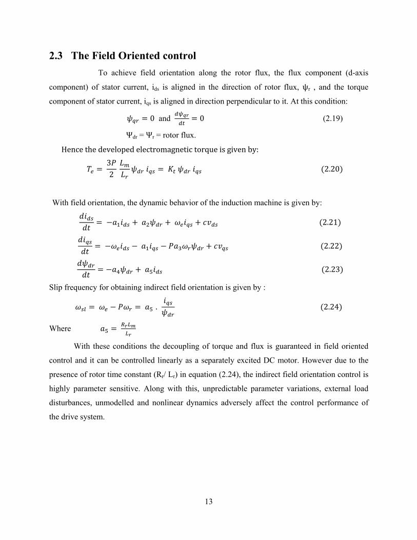
2.3 The Field Oriented control To achieve field orientation along the rotor flux, the flux component (d-axis

component) of stator current, ids is aligned in the direction of rotor flux, ψr , and the torque

component of stator current, iqs is aligned in direction perpendicular to it. At this condition:

0 and 0 (2.19)

Ψdr = Ψr = rotor flux.

Hence the developed electromagnetic torque is given by:

32 2.20

With field orientation, the dynamic behavior of the induction machine is given by:

2.21

2.22

2.23

Slip frequency for obtaining indirect field orientation is given by :

. 2.24

Where

With these conditions the decoupling of torque and flux is guaranteed in field oriented

control and it can be controlled linearly as a separately excited DC motor. However due to the

presence of rotor time constant (Rr/ Lr) in equation (2.24), the indirect field orientation control is

highly parameter sensitive. Along with this, unpredictable parameter variations, external load

disturbances, unmodelled and nonlinear dynamics adversely affect the control performance of

the drive system.

14

2.4 Estimation of Speed

It is desirable to avoid the use of speed sensors from the standpoints of cost, size

of the drive, noise immunity and reliability. So the development of shaft sensorless adjustable

speed drive has become an important research topic. Many speed estimation algorithms and

sensorless control schemes [22] have been developed during the past few years. The speed

information required in the proposed control technique is estimated by the algorithm described

in this section. The speed of the motor is estimated by estimating the synchronous speed and

subtracting the command slip speed. The synchronous speed is estimated using the stator flux

components, because of its higher accuracy compared to estimation based on rotor flux

components.

The rotor speed of an induction motor is expressed in terms of synchronous and slip

(angular) frequencies is as follows:

The estimation of rotor speed is accomplished by an estimation of either synchronous, or slip

frequency, with the other being known. In the proposed speed estimation scheme, the

synchronous frequency is estimated and slip frequency is assumed as command. So the

estimated rotor speed of the sensorless drive is obtained from the above equation as:

Where,

ω r = estimated rotor frequency in rad/sec.

ω e = estimated synchronous frequency in rad/sec.

ω*sl = command value of slip frequency in rad/sec.

The estimated synchronous frequency is derived based on the rotor flux model, or the stator flux

model. The principles of both the methods are briefly explained bellow.

If ψβr and ψαr are the two components of the rotor flux vector in the stationary (α-β)

reference frame as shown in Fig. 2.1 (a), the electrical angle of the rotor flux vector is defined as:

tan

15

The derivative of this rotor flux angle (with respect to time) gives the instantaneous angular

frequency.

(a) (b)

Fig. 2.1 Phasor diagram for rotor and stator flux components

If ψβs and ψαs are the two components of the stator flux vector in the stationary (α-β) reference

frame as shown in Fig. 2.1(b) the electrical angle of the stator flux vector is defined as:

tan

The derivative of this rotor flux angle (with respect to time) gives the instantaneous angular

frequency.

From the basic equation of induction motor in stationary (α-β) reference frame, the stator and

rotor flux linkages are given by

2.25

2.26

β

α

ψβr

ψαr

Ψr

θψr

β

α

ψβs

ψαs

Ψs

θψs

16

Equation (2.25) shows that the stator flux depends on the stator resistance and measured stator

voltages and currents. Equation (2.26) shows that the rotor flux depends on the estimated stator

flux and requires the knowledge of the inductances of the machine, especially the stator leakage

inductance (σ Ls). Usually the stator resistance can be measured fairly accurately. Hence stator

flux can be estimated more accurately compared to the rotor flux. Therefore the estimated stator

flux can be used to derive the synchronous frequency.

The block diagram of the described speed estimation algorithm with the sensorless speed

control scheme is shown in fig 2.2

Fig 2.2 Induction motor drive system with sensorless speed control scheme

From the

machine

terminal

1

1

Frequency

Estimator

3-phase

to

2-phase

transformation

T

1

2-phase To

3-phase Transformation

PWM

Inverter

Diode Rectifier

3 phase,

50 Hz

supply

IM

17

2.5 Chapter Conclusion

In this chapter the induction motor model in arbitrary reference frame is discussed in

detail. Because a dynamic model of the machine subjected to control must be known in order to

understand and design vector controlled drives. Condition to achieve indirect vector control is

derived. The speed estimation algorithm is studied in detail in order to apply the sensorless

technique in the present drive system.

18

Chapter – 3

DESIGN OF A SLIDING MODE CONTROLLER

3.1 Introduction In control theory sliding mode control, is a form of variable structure control (VSC). It

is a nonlinear control method that alters the dynamics of a nonlinear system by application of a

high-frequency switching control. The multiple control structures are designed so that

trajectories always move toward a switching condition, and hence the ultimate trajectory will not

exist entirely within one control structure. Instead, the ultimate trajectory will slide along the

boundaries of the control structures. The motion of the system as it slides along these boundaries

is called a sliding mode.

Intuitively, for a dynamic system sliding mode control uses practically infinite gain to

force the trajectories to slide along the restricted sliding mode subspace. The main strength of

sliding mode control is its robustness. Because the control can be as simple as a switching

between two states (e.g., "on"/"off" or "forward"/"reverse"), it need not be precise and will not

be sensitive to parameter variations that enter into the control channel. Additionally, because the

control law is not a continuous function, the sliding mode can be reached in finite time (i.e.,

better than asymptotic behavior). Sliding mode control is an appropriate robust control method

for the systems, where modeling inaccuracies, parameter variations and disturbances are present.

It is computationally simple compared to adaptive controllers with parameter estimation.

Induction motor with sliding mode control performs well in the servo applications, where the

actuator has to follow complex trajectories. Sometimes sliding mode control has a demerit of

chattering of the control variable and some of the system states.

The strengths of SMC include: • Low sensitivity to plant parameter uncertainty • Greatly reduced-order modeling of plant dynamics • Finite-time convergence (due to discontinuous control law)

19

The weaknesses of SMC include:

• Chattering due to implementation imperfections

3.2 sliding Mode Controller

With sliding mode controller, the system is controlled in such a way that the error in the

system states always moves towards a sliding surface. The sliding surface is defined with the

tracking error (e) of the state and its rate of change (e˙) as variables. The distance of the error

trajectory from the sliding surface and its rate of convergence are used to decide the control input

(u) to the system. The sign of the control input must change at the intersection of the tracking

error trajectory with the sliding surface. In this way the error trajectory is always forced to move

towards the sliding surface.

The basic equations (2.20 – 2.24) of vector controlled induction motor are simplified by

assuming, the rotor flux ψdr to be constant. From (2.23) the steady state value of the rotor flux

can be obtained as

3.1

From (2.15a), we get

3.1

Using (3.1a) in (3.1), steady state value of rotor flux is obtained as

3.1

The speed dynamic equation is given by

1

3.2

Using (2.20) in (3.2) we get,

20

Assuming the load torque, Tl to be a disturbance to a system, the speed dynamic equation is

simplified as:

3.3

or

3.3

Where,

3.4

and

3.4

In this vector controlled induction motor drive, speed is taken as the output variable. To track the

speed accurately in the second order speed control system, the conditions to be satisfied are:

0 0 3.5

From equation (4.2)

3.5

Substituting . in (2.22), the following equation is obtained.

3.6

It can be shown using (2.24) and (3.1), that

Simplifying (3.6), we get

1

or

3.6

Where

1 3.7

Substituting (3.2) and (3.6a) in (3.5a), we get

21

or

3.8

Where d = total disturbance

and u = b c vqs = control input. (3.8a)

and 3.9

G is a function, which can be estimated from measured values of current and speed.

u is directly proportional to vqs and decides the modulating signal and hence output voltage of the

PWM voltage source inverter.

Let

∆ 3.10

Where is an approximate estimate of G, and ΔG is the estimation error due to modeling

imperfection.

The control problem is to obtain the system states,

to track a specific time varying state,

in the presence of modeling imperfection and disturbances.

Let 3.11

and 3.12

be the tracking error in the speed and its rate of change respectively.

Let be the tracking error vector.

A time varying surface, s(t) is defined in the state space by the scalar equation ,

, 0

Where , 3.13

22

Where λ is a positive constant, which determines the band width of the system.

Starting from the initial condition, E(0) = 0, the tracking task, X X*, which means x

has to follow X* with a predefined precision, is considered as solved, if the state vector, E

remains in the sliding surface, S(t) for all t ≥ 0 and also implies that scalar quantity s is kept at

zero. A sufficient condition for this behavior is to choose the control law, u of (3.8) and (3.8a) so

that

12 | | 3.14

Where η is a positive constant. The value of η determines the degree to which the system state is

attracted to the switching line. Essentially, equation (3.14) states that the squared distance to the

sliding surface, as measured by s2 decreases along all system trajectories. Thus it constrains the

trajectories to point towards the surface S(t), as shown in the figure bellow [11].

Fig.3.1 The sliding condition

For a second order system, the switching surface is a line and different control structures

are applied according to the position of the tracking error vector with respect to the line. The

control is designed to drive the state in to the switching line, and once in the line the system state

is considered to remain on the line. The state trajectory is defined by the algebraic equation of

the line.

S(t)

23

Equation (3.14) is the ‘sliding condition’. S(t) satisfying (3.14) is referred to as a sliding

surface. And the behavior of the system, once on the surface is called ‘sliding mode’.

Graphical interpretation of equations (3.13) and (3.14) is shown in Fig. 3.2

Fig. 3.2 Graphical interpretation of equation (3.13) and (3.14)

Starting from any initial condition, the state trajectory reaches the sliding surface in a

finite tine smaller than | |, and then slides along the surface towards X* exponentially with a

time constant equal to 1/λ. In the sliding mode, behavior of the system is invariant despite

modeling imperfections, parameter variation and disturbances. However the sliding mode causes

drastic changes of the control variable, which is a major drawback for the system.

Slope λ

Sliding mode exponential convergence

X(0)

X(t)

S= 0

Finite time reaching phase

24

3.2.1 Derivation of Control Law

Referring to equation (4.13), the condition for sliding mode is

. | |

or alternatively, . 3.15

where

1 01 0

From equation (4.12) and (4.11)

3.16

Substituting (3.8) in (3.16),

3.17

Substituting (4.16) in (4.14) and simplifying,

. 3.18

To achieve the sliding mode of (4.14), u is chosen, so that

. 3.19

Where the gain, K is a positive constant. The first term in (3.19), is a compensation

term and second term is the controller. The compensation term is continuous and reflects the

knowledge of system dynamics. The controller term is discontinuous and ensures the sliding to

occur.

3.2.2 Design of Controller Gain

Substituting (4.18) in (4.17), we have

3.20

or

|∆ | | | 3.21

Where,

|∆ | = upper bound of the estimation error,

| | = upper bound of the noise, d, and

v = upper bound of command acceleration,

25

The controller gain K is determined from the maximum amount of imperfection in the estimation

process and maximum noise due to parameter variations and disturbance (load torque). If

modeling imperfection and parameter variation is large, the value of K should be large. Then

discontinuous or switched component . has a more dominant role than the continuous

or compensation component, and lead to chattering. Conversely, better knowledge of

the system model and parameter values reduces gain, K and results smooth control response. If

large control bandwidth is available, poor knowledge of dynamic model may lead to respectable

tracking performance, and hence large modeling efforts may produce only minor improvement in

tracking accuracy.

3.2.3 Reduction of Chattering

In a system, where modeling imperfection, parameter variations and amount of noise are

more, the value of K must be large to obtain a satisfactory tacking performance with sliding

mode controller. But larger value of K leads to more chattering of the control variable and

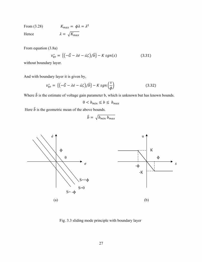
system states. A boundary layer of definite width on both sides of switching line is introduced to

reduce chattering. If is the width of the boundary layer on either side of the switching line, as

shown in fig. 3.3, the control law of (3.19) is modified as:

. 3.22

Where

| |

| |

This accounts to a reduction of the control gain inside the boundary layer and results in a smooth

control signal.

26

3.2.4 Design of Bandwidth, λ

From equation (4.21), for | | , ( )

∆ 3.23

Substituting equation (3.23) in (3.17), the filter function is obtained as

∆ 3.24

Where d is the disturbance and ΔG is the model imperfection.

Suppose the solution of the filter equation (3.24) is s0 . Then the distance from the state vector, E

to the switching line, s=0 is:

| | 1

√1 3.25

Since slope of the switching line, s=0 is λ, the guaranteed tracking precision is:

3.26

The break frequency, υ of filter (3.24) is:

3.27

The design rule for bandwidth, λ is that the largest acceptable value of λ should be more than or

equal to the break frequency, υ of filter (3.24). From (3.27) the balance condition is obtained as:

3.28

This case corresponds to critical damping. Further more the design rule for λ with regard to

sample rate, fsample and time constant, τplant of the plant is denoted as

2 1 . 3.29

λ is selected keeping equations (3.26), (3.28) and (3.29)in view. The ratio of boundary layer ( )

to bandwidth (λ) should be as small as possible, the ratio being equal to specified tracking

precision. There product should be equal to the maximum value of controller gain, Kmax . If time

constant of the system is known, λ should satisfy (3.29).

To have a tracking precision, θ = 1 rad/sec, from (3.26)

3.30

27

From (3.28)

Hence

From equation (3.8a)

/ 3.31

without boundary layer.

And with boundary layer it is given by,

/ 3.32

Where is the estimate of voltage gain parameter b, which is unknown but has known bounds.

0

Here is the geometric mean of the above bounds.

(a) (b)

Fig. 3.3 sliding mode principle with boundary layer

S=+

S=0 S= -

θ

u

‐

K

‐K

28

Fig. 3.4 Induction motor drive system with sliding mode controller

3.3 Chapter Conclusion

In this chapter the theory of sliding mode controller is briefly reviewed. The equations in

the induction motor model are reorganized so as to apply the control technique. The controller

gain and bandwidth are designed, considering various factors such as rotor resistance variations,

model inaccuracies, load torque disturbance, to have ideal speed tracking. In the next chapter the

simulation results are presented and discussed to validate the proposed control scheme.

1

Frequency

Estimator

3-phase

to

2-phase

transformation

T

2-phase To

3-phase Transformation

PWM

Inverter

Diode Rectifier

3 phase,

50 Hz supply

G1 Sliding

Mode

Controlle

ue

IM

29

Chapter – 4

SIMULATION RESULTS AND DISCUSSIONS

The induction motor drive system is simulated with (i) P-I controller and (ii) sliding

mode controller in the mechanical subsystem. Both the controllers are tested for speed tracking

and load torque variation conditions. Results are compared among both types of controllers. The

drive is subjected to load disturbance to test the robustness of the sliding mode controller.

The rating and parameters of a 3-phase induction motor drive system are given in Appendix –A.

Different cases under which the simulation tests are carried out are:

(a) Step change in reference speed.

(b) Tracking of reference speed in trapezoidal form.

(c) Robustness test against load torque variation.

The comparative study of the results with P-I and SMC are shown bellow.

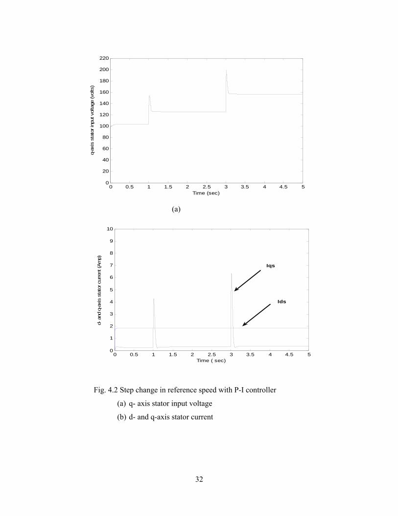
(a) Step change in reference speed

The reference speed is changed from 1000 rpm to 1200 rpm at time, t = 1 sec, and again 1200

rpm to 1500rpm at time, t = 3 sec. The reference d-axis rotor flux linkage is kept at 0.45

V.sec and load torque is kept at zero. The simulation responses of the drive system with P-I

controller are shown in Fig. 4.1, Fig. 4.2 and Fig. 4.3 and those with sliding mode controller

are shown in Fig. 4.4, Fig 4.5 and Fig. 4.6. The responses of speed, speed error, d- and q-axis

stator currents, stator phase current (ia), the control voltage (‘u’ in SMC) and q-axis stator

input voltage (Vqs) are shown.

From the figures it is clear that in case of sliding mode controller, the speed error of the

system comes to zero faster than fixed gain controller. The q-axis input voltage at the time of

transition from one level to anther is nearly 20times larger in case of sliding mode controller

30

than P-I controller. Similarly the q-axis stator current is much larger in case of sliding mode

controller than P-I controller.

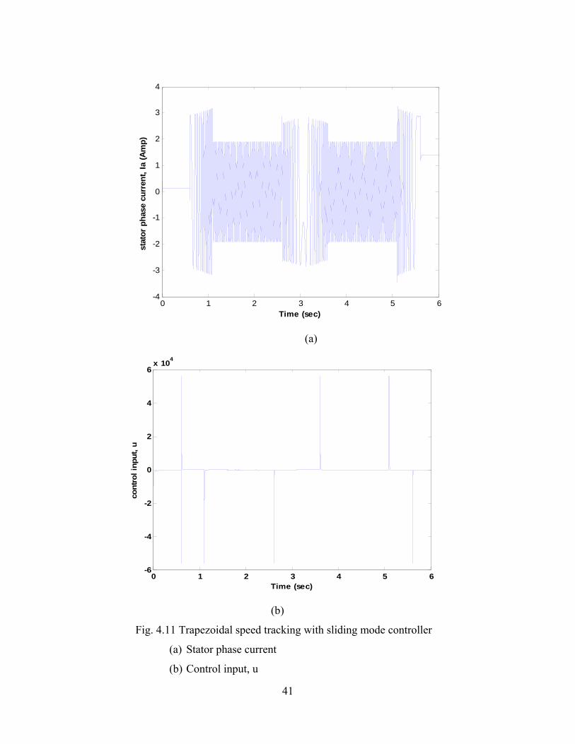
(b) Tracking of reference speed in trapezoidal form.

A periodic trapezoidal reference speed is used here to study the tracking performance of

the drive system. It is shown in Fig. 4.7 and Fig. 4.8 for fixed gain P-I controller and Fig. 4.9,

Fig. 4.10 and Fig. 4.11 for sliding mode controller. The command speed is increased linearly

from 0 at t = 0.6 sec to 157rad/sec at t = 1.1 sec. It is kept constant at 157rad/sec till t = 2.6 sec,

and decreased linearly to -157rad/sec at t = 3.6 sec. Then command speed is kept constant at -

157rad/sec till t = 5.1sec and increased linearly to zero at t = 5.6 sec. Same trajectory is used to

study the performance of fixed gain P-I controller and sliding mode controller, and results are

compared.

Compared to P-I controller the speed tracking performance of sliding mode controller is

much better. For both the cases, the q-axis stator voltage, d-and q-axis stator current are shown

in the figure. For the sliding mode controller the control input is also shown in the figure.

Fig. 4.12 shows the responses of the controllers during variation of load torque. It is clear

that the P-I controller speed response is affected by the load disturbance, where as the sliding

mode controller has proved its robustness against load variations.

31

(a)

(b)

Fig. 4.1 Step change in reference speed with P-I controller

(a) Speed ,

(b) Speed error,

0 0.5 1 1.5 2 2.5 3 3.5 4 4.5 50

20

40

60

80

100

120

140

160

Time in sec

spee

d in

rad/

sec

0 0.5 1 1.5 2 2.5 3 3.5 4 4.5 5-5

0

5

10

15

20

25

30

35

Time (sec)

Spe

ed e

rror (

rad/

sec)

32

(a)

Fig. 4.2 Step change in reference speed with P-I controller

(a) q- axis stator input voltage

(b) d- and q-axis stator current

0 0.5 1 1.5 2 2.5 3 3.5 4 4.5 50

20

40

60

80

100

120

140

160

180

200

220

Time (sec)

q-ax

is s

tato

r inp

ut v

olta

ge (v

olts

)

0 0.5 1 1.5 2 2.5 3 3.5 4 4.5 50

1

2

3

4

5

6

7

8

9

10

Time ( sec)

d- a

nd q

-axi

s st

ator

cur

rent

(Am

p)

Iqs

Ids

33

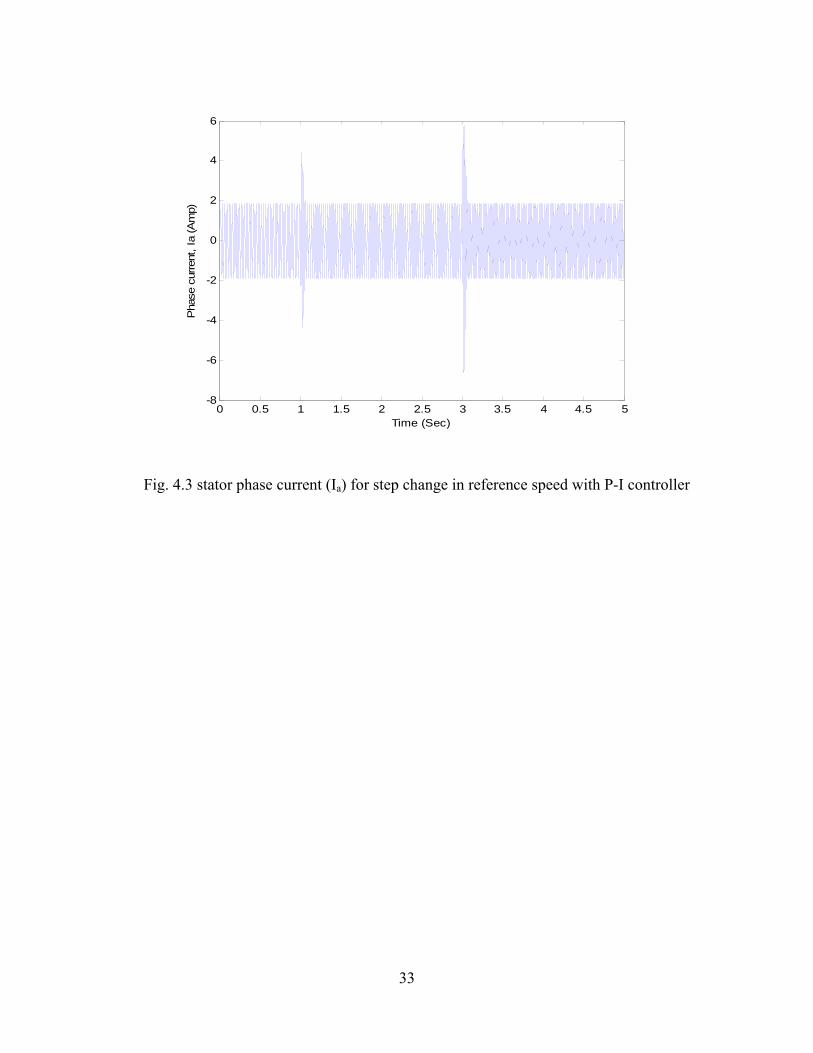
Fig. 4.3 stator phase current (Ia) for step change in reference speed with P-I controller

0 0.5 1 1.5 2 2.5 3 3.5 4 4.5 5-8

-6

-4

-2

0

2

4

6

Time (Sec)

Pha

se c

urre

nt, I

a (A

mp)

34

(a)

(b)

Fig. 4.4 Step change in reference speed with sliding Mode controller

(a) Speed ,

(b) Speed error,

0 0.5 1 1.5 2 2.5 3 3.5 4 4.5 50

20

40

60

80

100

120

140

160

Time (sec)

Spe

ed (r

ad/s

ec)

0 0.5 1 1.5 2 2.5 3 3.5 4 4.5 5-5

0

5

10

15

20

25

30

35

Time (Sec)

Spe

ed E

rror (

rad/

sec)

35

(a)

(b)

Fig. 4.5 Step change in reference speed with sliding mode controller

(a) q- axis stator input voltage

(b) d- and q-axis stator current

0 0.5 1 1.5 2 2.5 3 3.5 4 4.5 50

500

1000

1500

2000

2500

3000

3500

4000

Time (sec)

q-ax

is s

tato

r inp

ut v

olta

ge (v

olts

)

0 0.5 1 1.5 2 2.5 3 3.5 4 4.5 5-10

0

10

20

30

40

50

60

Time (sec)

d- a

nd q

-axi

s st

ator

inpu

t cur

rent

(Am

p)

Iqs

Ids

36

(a)

(b)

Fig. 4.6 Step change in reference speed with sliding Mode controller

(a) Stator phase current in Amp

(b) Control input, u in rad/s3

0 0.5 1 1.5 2 2.5 3 3.5 4 4.5 5-10

-5

0

5

10

15

20

25

30

35

Time (sec)

stat

or p

hase

cur

rent

, Ia

(Am

p)

0 0.5 1 1.5 2 2.5 3 3.5 4 4.5 5-6

-4

-2

0

2

4

6x 104

Time (Sec)

Cont

rol I

nput

, u

37

(a)

(b)

Fig. 4.7 Trapezoidal speed tracking with P-I controller

(a) Speed response

(b) q-axis stator voltage

0 1 2 3 4 5 6-200

-150

-100

-50

0

50

100

150

200

Time ( sec)

Spee

d (r

ad/s

ec)

0 1 2 3 4 5 6-200

-150

-100

-50

0

50

100

150

200

Time (sec)

q-ax

is s

tato

r vo

ltage

(vol

ts)

38

(a)

(b)

Fig. 4.8 Trapezoidal speed tracking with P-I controller

(a) d- and q-axis stator current

(b) stator phase current

0 1 2 3 4 5 6-3

-2

-1

0

1

2

3

Time (sec)

d- a

nd q

-axi

s st

ator

cur

rent

(am

p)

Ids

Iqs

0 1 2 3 4 5 6-4

-3

-2

-1

0

1

2

3

4

Time (sec)

stat

or p

hase

cur

rent

, Ia

(Am

p)

39

(a)

(b)

Fig. 4.9 Trapezoidal speed tracking with sliding mode controller

(a) Speed response

(b) Speed Error

0 1 2 3 4 5 6-200

-150

-100

-50

0

50

100

150

200

Time (Sec)

Spe

ed (r

ad/s

ec)

0 1 2 3 4 5 6-0.8

-0.6

-0.4

-0.2

0

0.2

0.4

0.6

Time (Sec)

Spee

d Er

ror (

rad/

sec)

40

(a)

(b)

Fig. 4.10 Trapezoidal speed tracking with sliding mode controller

(a) q-axis stator voltage

(b) d- and q-axis stator current

0 1 2 3 4 5 6-200

-150

-100

-50

0

50

100

150

200

Time (sec)

q-ax

is s

tato

r vo

ltage

(vol

ts)

0 1 2 3 4 5 6-3

-2

-1

0

1

2

3

Time (sec)

d- a

nd q

-axi

s st

ator

cur

rent

(Am

p)

Ids

Iqs

41

(a)

(b)

Fig. 4.11 Trapezoidal speed tracking with sliding mode controller

(a) Stator phase current

(b) Control input, u

0 1 2 3 4 5 6-4

-3

-2

-1

0

1

2

3

4

Time (sec)

stat

or p

hase

cur

rent

, Ia

(Am

p)

0 1 2 3 4 5 6-6

-4

-2

0

2

4

6x 104

Time (sec)

cont

rol i

nput

, u

42

(a)

(b)

Fig: 4.12 Performance of the drive system under load torque variation

(a) With P-I controller

(b) With Sliding Mode controller

0 1 2 3 4 5 6-200

-150

-100

-50

0

50

100

150

200

Time (Sec)

Spee

d (ra

d/se

c) a

nd L

oad

Torq

ue (N

.m)

0 1 2 3 4 5 6-200

-150

-100

-50

0

50

100

150

200

time (Sec)

Spee

d (ra

d/ S

ec) a

nd L

oad

Torq

ue (N

.m)

43

Chapter- 5

CONCLUSION AND FUTURE WORK

In this thesis the theory of sliding mode controller is studied in detail. The equations

of the induction motor model are reorganized so as to apply the control technique. The controller

gain and band width are designed, considering various factors such as rotor resistance variation,

model in accuraies, load torque distrubance and also to have an ideal speed tracking. Considering

the case such as load disturbance, the response of the designed sliding mode controller is

satisfactory. It also gives good trajectory tracking performance. The speed regulation characteristic

is also satisfactory.

Only load distrubance is the problem considered in this case and the robustness of the

controller is verified. Since the machine rating is small, the resistance variation effect is very

small. Hence has negligible effect. As a future work this controller can be applied to any other

drive system with higher rating where parameter variation effect can be studied. Fuzzy logic

Principle can be incorporated to this controller to make it more efficient and robust.

44

REFERENCES

[1] Bose B.K.,”Modern Power Electronics and AC Drives”, Pearson Education, 4th

Edition, 2004

[2] R.M. Cuzner, R.D. Lorenz, D.W. Novotny, “Application of non-linear observers for rotor

position detection on an induction motor using machine voltages and currents,” IEEE-

IAS Annual Meeting Conference Record, October 1990, pp. 416–421.

[3] Atkinson D. J., P. P. Acarnley and J. W. Finch, “Application of estimation technique in

vector controlled inductin motor drives,” IEE Conference Proceeding, London, July

1990, pp. 358-363.

[4] A. Ferrah, K.G. Bradely, G.M. Asher, “Sensorless speed detection of inverter fed

induction motors using rotor slot harmonics and fast Fourier transform,” IEEE-PESC

Conference Record, October 1992, pp. 279–286.

[5] Baader U., M. Depenbrock, and G. Gierse, “ Direct self control of inverter- fed induction

machines: A basis for speed control without a speed measurement,” IEEE Trans. Ind.

Appl., vol. 28, no. 3, May 1992, pp. 581-588.

[6] Blaschke F., “ The principle of field orientation as applied to the new TRANSVECTOR

closed loop control system for rotating field machines,” Siemens Review, vol. 93, no.

5,may 1970, pp. 217-220.

[7] Chan, C. C., and H. Q. Wang, “New scheme of sliding mode control for high

performance induction motor drives,” IEE Proc. on Electric Power Applications, vol.

143, no. 3, May 1996, pp 177- 185.

[8] Chan C. C., Leung W. S. and C. W. Nag, “ Adaptive decoupling control of induction

motor drives,” IEEE Transaction on Industrial Electronics, vol. 35, no. 1, Feb. 1990,

pp.41-47.

[9] N. Teske, G.M. Asher, M. Sumner, K.J. Bradely, “Suppression of saturation saliency

effects for the sensorless position control of induction motor drives under loaded

conditions,” IEEE Trans. Ind. Appl. 47 (5) (2000) 1142–1150.

45

[10] N. Teske, G.M. Asher, M. Sumner, K.J. Bradely, Encoderless position estimation for

symmetric cage induction machines under loaded conditions, IEEE Trans. Ind. Appl. 37

(6) (2001) 1793–1800.

[11] Dunngan, M. W., S. Wade, B. W. Willams, and X. Xu, “Position control of a vector

controlled induction machine using Slotine’s sliding mode control approach,” IEE Proc.

on Elect. Power Appl., vol. 145, no. 3, May 1998, pp. 231- 238.

[12] Garces L. J., “Parameter adaptation for speed controlled static AC drives with a squirrel

cage induction motor,” IEEE Trans. On Industry Applications, vol. 16, no. 12, Mar. 1980,

pp 173 -178.

[13] Hasse K., “ On the dynamic behavior of induction machines driven by variable frequency

and voltage sources,” ETZ Arch. Bd. 89, H. 4, 1968, pp. 77-81.

[14] Hung K. T., and R. D. Lorenz, “ A rotor flux error based adaptive tuning approach for

feed forward field oriented induction machine drives,” IEEE Conf. record IAS annual

meeting, 1990, pp. 594-598.

[15] Kim Y. R., S. K. Sul and M.H. Park, “ Speed sensorless vector control of induction motor

using extended Kalman filter,” IEEE Transaction on Ind. Appl., Vol. 30, no. 5, 1994, pp.

1225-1233.

[16] Krause P. C., Analysis of Electric Machinary, McGrow-Hill, New York, 1986

[17] Krause P. C and C. S. Thomas, “Simulation of symmetrical induction machinery,” IEEE

Trans. on Power Apparatus & Systems, vol. 84, no. 11, 1965, pp. 1038- 1053.

[18] Krishnan R. and A. S. Bharadwaj, “ A review of parameter sensitivity and parameter

deviations in feed forward field oriented drive systems,” IEEE Transaction on power

Electronics, vol.6, no. 4, 1991, pp. 695- 703.

[19] Mohanty K. B., A. Routray and N. K. De, “Rotor flux oriented sensor less induction

motor drive for low power applications.” Proceeding of Int. Conference on Computer

Application in Electrical Engg.: Recent Advances (CEERA), Feb, 2001, Roorkee, pp.

747- 752

[20] Nilsen R. and M. P. Kazmeirkowski, “ Reduced order observer with parameter adaptation

for fast rotor flux estimation in induction machin,” IEE Proceeding, vol. 136, no. 1, Jan.

1989, pp. 35-43.

46

[21] Park, T. G., and K. S. Lee, “SMC based adaptive input-output linearizing control of

induction motors,” IEE Proc. on Control Theory Applications, vol. 145, no. 1, Jan 1998,

pp. 55-62.

[22] Rajsekhar K., A. Kawamura, and K. Matsuse, “Sensorless control of AC motor drives:

Speed and Position sensorless operation,” Piscataway, NJ, IEEE press, 1996.

[23] Soto, R., and K. S. Yeung, “ Sliding mode control of induction motor without flux

measurement,” IEEE Transaction on Industrial Application, vol. 31, no. 4, 1995, pp.744-

751.

[24] Tajima H. and Y. Hori, “ Speed sensorless field oriented control of induction machine,”

IEEE Transaction on Industrial Application, vol. 29, no. 1, 1993, pp.1003-1008

[25] Utikin, V. I., “ Variable structure system with sliding mode: A Survey,” IEEE

Transaction on Automatic control, vol. 22, no, 2, 1977, pp. 212-222

[27] Zhen L., and L. Xu, “ sensorless field orientation control of induction machines based on

a mutual MRAS scheme,” IEEE Transaction on Industrial Electronics, vol.45, no. 5, Oct.

1998, pp824-831.

[28] Benchaib, A., A. Rachid, and E. Audrezet, “ Sliding made input-output linearization and

field orientation for real time control of induction motors,” IEEE Trans. on Power

Electronics, vol. 14, no.1, Jan 1999, pp.128- 138.

[29] Benchaib, A., A. Rachid, E. Audrezet, and M. Tadjine, “Real time sliding mode observer

and control of an induction motor,” IEEE Trans. on Ind. Electronics, vol. 46, no. 1, Feb

1999, pp. 128-138.

[30] Mohanty K.B., “Sensorless sliding mode control of induction motor drives,” TENCON-

2008, IEEE Region 10 Conference, Hyderabad.

[31] A. Derdiyok, M. K.Guven, Habib-Ur Rahman and N. Inane, “Design and Implementation

of New Sliding-Mode Observer for Speed- Sensorless Control of Induction Machine,”

IEEE trans. on Industrial Electronics, Vol. 1, No.3, 2002.

[32] Barambones, O. and Ggarrido, A.J, “A sensorless variable structure control of induction

motor drives,” Electric Power systems Research, 2004, pp 21-32

47

APPENDIX- A

Parameters of Typical Induction Machine

Three phase, 50 Hz, 0.75kW, 220V, 3A, 1440rpm

Stator Resistance Rs = 6.37Ω

Rotor resistance Rr = 4.3Ω

Stator inductance Ls = 0.26H

Rotor Inductance Lr = 0.26H

Mutual Inductance Lm = 0.24 H

Number of Poles P = 4

Moment of inertia of motor and load J = 0.0088Kg.m2

Viscous friction coefficient B = 0.003 N.m.s/rad

Proportional cum Integral controller parameters

Speed loop PI controllers

KP1 = 0.35 KI1 = 1

KP2 = 100 KI2 =29877

Flux loop PI controller

KP3 = 151.27 KI3 = 43649