a simple model of information use in the exploitation of patchily distributed food

Anim. Behav., 1985, 33, 553-560

A simple model of information use in the exploitation of patchily distributed food

JOHN M c N A M A R A * & A L A S D A I R H O U S T O N t *School of Mathematics, University of Bristol, Bristol U.K.

~fDepartment of Zoology, University of Cambridge, Downing Street, Cambridge, U.K.

Abstract. In this paper we consider a simple model of an environment in which prey are distributed in patches. It is assumed that each patch contains at most one item, but items may vary in the ease with which they can be found. The time spent in unsuccessful search on a patch gives information of whether a patch contains an item, and if it does, how difficult that item is to find. We show how this intbrmation can be used to find the policy which maximizes the mean rate of reward for the environment. The analysis is illustrated by two examples.

The marginal value theorem (Charnov 1976) gives a simple criterion for an animal to leave a patch if it is to maximize its overall rate of energetic gain. Briefly stated, the animal should leave when the instantaneous rate of intake in the patch drops to the overall rate for the environment. The simplicity of this result is bought at the cost of some restrictive assumptions about the foraging process. The cumulative energetic gain while on the patch is assumed to be a smooth decelerating function of time on the patch. Perhaps more importantly, the animal does not gain any information while foraging. Oaten (1977) raised these issues shortly after Charnov's work was published, but although pious reference is made to Oaten's paper, it does not seem to have made a fundamental change to people's thinking about patch-use problems. Although Oaten's argument can be put in a more general and intuitive context (McNamara 1982) the difficulty of the mathematics is still something of a barrier to the fieIdworker. In an attempt to remove the barrier, this paper presents some examples of how to calculate reward rate on the patch when rewards occur as discrete items. We also illustrate the optimal policy when the time to find a reward gives the forager information. The analysis is kept simple by confining attention to problems in which there is never more than one reward item per patch. The general environment we consider is one in which patches may vary in both the number of prey items present (zero or one) and in the difficulty of finding an item if one is present. A searching animal's sole indicator of patch quality is assumed to be the time spent on the patch so far.

It is clear that the optimal policy for such a

problem has the form 'leave as soon as a reward is found or after a certain duration of unsuccessful search'. We find this duration, which we refer to as the maximum time on patch, in the general case. We then apply the analysis to two special cases. In the first case, all prey are equally easy to find, but only some of the patches contain a prey item. Unsuccessful search in a patch of this environment indicates that it is likely that the patch is empty. It therefore becomes optimal to leave after a certain time.

In the second case, all patches contain exactly one item, but items vary in how easy they are to find. Unsuccessful search now makes it likely that the current patch contains an item which is hard to find, and again it eventually becomes optimal to leave without a reward. We illustrate such a case by considering patches to be nuts. The nuts vary in the ease with which they can be opened, and the longer the forager has been trying to open the nut, the more likely it is that the nut is a hard one.

THE T I M E TO FIND A PREY I T E M

The forager's ability to exploit a patch is given by the distribution of the time to find a reward. This distribution will depend on many factors, such as the crypticity of the prey and the predator's search strategy.

Let Xbe the time to find a reward on a randomly selected patch. The distribution function F(x) of X gives the probability that X will not be greater than x, i.e. F(x) = P(X<_x). In empirical studies F(x) can be found by plotting the cumulative probability that an item has been found as a function of the

553

554 Animal Behaviour, 33, 2

time spent searching. T~le data of Pietrewicz & Kamil (1981) on the behaviour of blue jays (Cyano- citta cristata) searching for moths could be treated in this way.

It must be emphasized that F(x) is the distribution on a randomly chosen patch. To illustrate the point, let all the patches contain exactly one item and let there be a constant probability of finding an item while searching. Then X has an exponential distribution and

F(x) = 1 - e -~x

so that the probability of capture tends to one. If, instead, a proportion q of the patches are empty, then the capture time will be infinite on the empty patches and exponential on the patches that contain a prey item. Therefore on an average patch,

F(x) = q - 0 + p ( 1 - - e ).x) (1)

where p = 1 - q . This now tends t o p as x increases.

G A I N I N G I N F O R M A T I O N A B O U T A P A T C H

When some patches do not contain a prey item, the time that has been spent waiting for an item can give the predator information about the likelihood of an item being present. Let a proport ion p of the patches contain a prey item. Thus on arrival at a randomly chosen patch, p is the a priori probability that the patch will contain an item. Consider first a forager that takes a fixed time D to find an item. In this case, waiting for time t < D gives the animal no additional information about patch type. Waiting for a time t > D gives the animal perfect information.

In mathematical terms, waiting for a time t without finding a reward means that X > t. In the example that we have just given, the reason that there is no information when t < D is that P(X> t) is the same for patches with and without an item. In general, these two probabilities will differ, and hence will provide additional information about patch type. Mathematically, this additional information can be combined with the a priori probability to give a posterior probability p(t) that the patch contains an item (see McNamara & Houston 1980).

From Bayes' theorem p(t) =

p- Probability X > t on patches that contain an item

Probability X > t on a randomly chosen patch

Denoting the probability X > t on patches that contain an item by PI (X> t), the posterior is given by the equation

p ' P I ( X > t) p(t) (2)

1 - F ( t ) To illustrate the calculation ofp(t), let us again

suppose that on patches that contain a prey item the time to find the item is exponentially distributed with parameter 2. Then P~(X> t ) = e ~-)x, and thus by equations (1) and (2)

P p(t) - - - (3) qe ~t + P

where q = 1--p. Note that as the time spent in unsuccessful search, t, increases, p(t) decreases and tends to zero.

Just as additional information can be used to update p to p(t) so one can update the probability density f ( t ) . On arrival at a patch the a priori probability that a reward will be found between search times t and t + 6, P(t < X < t + 6), is approximately f ( t )6 for small 6. If the animal searches unsuccessfully till time t this alters the probability of a reward between times t and t + 6. We define the reward rate r(t) so that this posterior probability is approximately r(t) ~ for small 6. To be more precise

Probability of a r(t) = limit reward between t and t + 6 given X > t

6~0 6

Since P(t < X < t+ 6) is simply the product of the numerator of this expression multiplied by P(X > t) we have

f ( t ) r(t) - (4)

1 --F(t)

It is the additional l - - F ( t ) term that takes into account the information that no reward has been found by time t.

Note that reward rate r(t) is defined in terms of future expectations rather than a smoothing over of previously obtained reward, a procedure that would be useless when patches contain at most one prey item.

T H E L O N G T E R M R E W A R D R A T E

Our optimality criterion is to maximize the overall (or long-term) reward rate ?. By renewal theory arguments (Johns & Miller 1963), ? is given by the expected reward on a patch divided by the expected time from leaving one patch to leaving the next patch. For the problems that we are considering,

McNamara & Houston." Patch use and information 555

the optimal policy has the form: leave a patch as soon as a reward is obtained, otherwise leave after a time t on the patch. We will refer to t as the maximum time on patch. For a policy of this form, the dependence of , /on t can be obtained as follows. F rom the definition of the distribution function,

expected reward on patch = F(t)

The expected time consists of two things, the expected time z taken to travel between patches and the expected patch residence time, E(Tt). Thus:

F(t) (5) 7, - E(T, )+ z

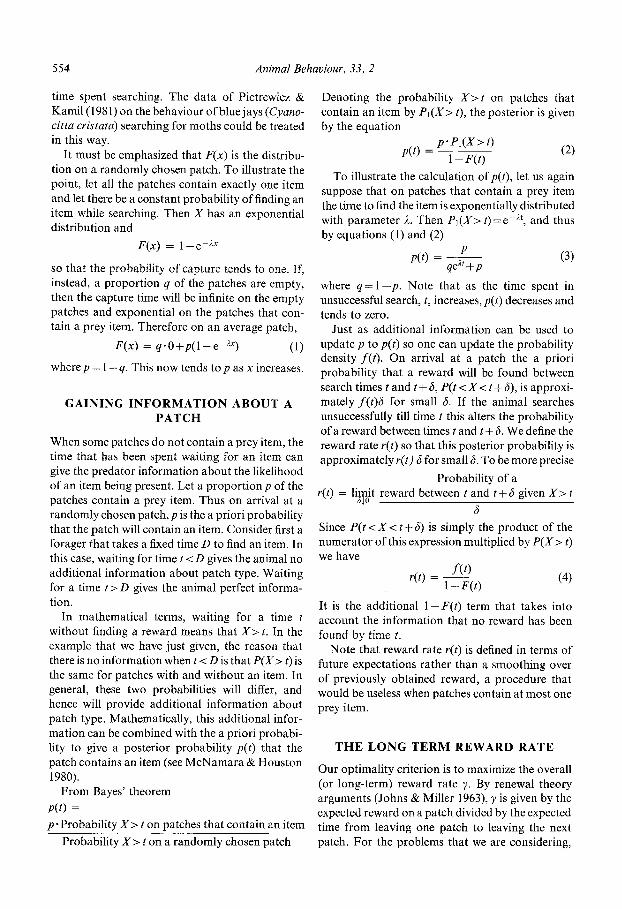
It might seem that F(t) can be used to construct the overall rate in the manner shown in Fig. 1, where F(t) is plotted against t. But the slope of the tangent AB is

F(tO

tl -+-z

which is not the overall rate, since t~ is not equal to E(Ttl). For any maximum time t,E(Tt) will be less than t since a reward may be found before time t. To derive an expression for the expected patch residence time, note that either the animal finds the reward before t or it gives up at t. The probability of finding a reward 'at ' x, where x is less than t, is f ( x ) = F'(x). The probability of giving up at t is 1--F(t). Thus:

E(Tt) = foXf(x)dx + t(1 - F ( t ) )

which integrates by parts to give

E(Tt) = t - l toF(x )dx (6)

Equat ion (6) means that the expected patch residence time is less than the maximum time in patch by the shaded area in Fig. 1. When F(x) is an

Expected B reward F (t I

-~ t l t z Maximum t ime on patch t

Figure l. The curve shows a hypothetical distribution function F(t). The figure illustrates that the optimal policy is not to employ a maximum time in patch tb This is because the slope of AB is not ?t~, since the mean patch residence time E(TtO is not equal to tb For a general maximum time on patch t2, the area of the shaded region equals the difference between t2 and E(Ttz).

empirically derived function, the optimal rate can be found by calculating yt as a function of t using equations (5) and (6). The value of t that maximizes 7t is then the optimal maximum time on patch t*, and the resulting value of yt is the maximum achievable rate 7*.

There are cases in which there is no maximum value of yr. For example, when all the patches contain just one item that is found after an exponential time, then

E(Tt) = t-- I' o (1-e- '~X)dx

Thus:

= ~(1-e -at)

(! - e -~') Y ~ - 1 ~+~(1 - e -~t)

Since this is an increasing function of t the optimal giving up time is 'infinite' and the optimal policy is to remain on each patch until a reward is found. This conclusion reinforces the argument that Fig. 1 does not give the correct procedure.

T H E E Q U A L R A T E S P R O C E D U R E

The optimal policy can often also be characterized in terms of the reward rate r(t). Oaten (1977) and McNamara (1982) show that when r(t) decreases with t it is optimal to leave without a reward when r(t) falls to 7*. Thus the stochastic analogue of Charnov's Marginal Value Theorem (Charnov 1976) holds in this case. (Note, however, that when patches may contain more than one prey item this equal rates procedure may not be optimal.)

Both the above characterizations of the optimal policy are illustrated in the following examples.

Constant Reward Rates

From a consideration of the stochastic reward rate r, it can be seen that it is never optimal to leave before a reward is found when r(t) is constant. The journey to a new patch wastes time, and the rate on the new patch will still be the same. The argument also holds when r(t) is increasing, as can happen when a finite patch is searched systematically by a predator that never misses an item. A problem of this sort is analysed by McNamara & Houston (1983).

A constant expected reward rate arises if the time


to a reward is exponential, i.e. F(x )= 1 - e -~-~ and f ( x ) =2e -)'x. In such a case equation (4) gives

he kx r(t) = ~ = 2

e

It is easy to see that the converse is also true, so that a constant rate on the patch is equivalent to an exponential distribution of time to reward.

In contrast to r(t), f ( t ) decreases with t. As we have explained r(t) is calculated a posteriori given that no reward has been found by time t, whereas

f ( t ) is an a priori probability of capture. It is r(t) that must be used to characterize the optimal policy since it is this quantity which is based on current information.

It is not clear what sort of search strategy in a finite patch would give rise to a constant stochastic rate, r. There is, however, a good example of such a reward rate that also illustrates the generality of the concept of a patch. Zach (1979) describes the way in which northwestern crows (Corvus eaurinus) drop whelk shells. He claims that a shell has a constant probability of breaking each time that it is dropped. Shells can be thought of as patches, and the number of drops can be thought of as search time (restricted to integer values). As Zach points out, once a crow has started dropping a shell, it is optimal to continue with it until it breaks. He found that crows behaved in this way, being very persist- ent in their attempts to break shells. Another possible example is that of predators such as flycatchers and kestrels that wait for a prey item to appear at a certain site.

As stated, both these possibilities require the predator to never give up before a reward is obtained. With only minor modifications, however, the problems become non-trivial, as the next two sections show.

S o m e Patches are Empty

The environment consists of two sorts of patches. Patches of one sort contain exactly one item whereas patches of the other sort are empty. Even if the time to wait for an item in the former class of patches is exponential, the optimal maximum time on patch is finite. As we have seen in the exponential case, when some patches may be empty the longer an animal has searched unsuccessfully for an item, the less likely it is that an item is present (see equation 3). Thus it eventually becomes optimal to leave the patch without a reward.

Let p be the proport ion of patches that are not empty and suppose that on these patches food is found after an exponential time with mean 1/2. To find the optimal policy in this case we derive an expression for 7t as a function of t. By equation (1)

t t So F(x)dx = pSo (1 -e- '~X)dx

1 = p ( t - - ~ ( 1 - e-~'))

Thus

E(Tt) = q t+~(1 ~ e m ~ t ~

where q = 1 - p , so that

�9 p ( l - - e -~') 7t

+ qt +2(1 -- e -~t) "C

Table I shows the optimal values of t and the corresponding values ofyt as a function o f z and q.

By equations (4) and (1)

P2e-~' (7) r(t) - q+pe_)~t

Thus by equation (3)

r(t) = 2p(t)

so that r(t) tends to zero as t increases. It may be verified that r ( t*)=?*: for example when q=0 .5 and ~ =0.5, Table I shows that t* - 1.146. Formula (7) shows that r(t*)= 0-24l, which is the value of y* shown in the table.

Table I. Optimal maximum time in patch t* and reward rate ?* as a function of travel time r when a proportion q of the patches are emptyt

z t* 7" q

0"5 2"091 0'527 0"1 1-146 0"241 0"5 0.897 0"043 0'9

1.0 2-611 0-398 0-I 1.505 0.182 0.5 1.196 0.033 0.9

2.0 3.186 0.271 0.1 1.937 0-126 0.5 1-566 0.023 0.9

3.0 3.542 0.207 0.1 2.222 0.098 0.5 1.816 0.018 0-9

t k = l .

McNamara & Houston. Patch use and information 557

This example is relevant to the results reported by Kamil (1983). Blue jays were presented with slides o f birch trees, some of which had a moth (Catocala relicta) on them. These correspond to patches that contain a prey item. A jay is presented with the slides in an operant procedure. When a given slide is projected, the bird can peck either an 'a t tack ' key or a 'reject' key. I f it pecks the reject key, there is a 2-s delay after which the next trial begins with a further delay to represent travel time. If it pecks the attack key there is a 30-s delay (to represent approach and handling) after which a piece of mealworm is delivered if and only i fa moth was present. After a further 2 s, the next trial begins with a travel time.

Kamil (1983) refers to the maximum time on the patch as the giving-up time, measured by the latency to reject a slide. He found some evidence for an increase in maximum time on patch with increasing travel time, as is required under the opt imal policy. He also found an increase in the probabili ty of finding a moth on slides containing a moth. This is a simple consequence of the increase in t* with z.

Two findings are outside the scope of our model. As travel time increases, jays reduce attack latency and (probably as a result) increase the number of incorrect attacks on slides without moths. Our current approach requires that the forager only attacks when a prey item is present. We hope to develop a less restrictive model that incorporates detection errors.

certain time. Grieg-Smith (in press) reports that bullfinches, Pyrrhula pyrrhula, show such behaviour, and so do great tits, Parus major (personal observation).

To formalize this idea we make the following assumptions: (1) each seed has an associated positive parameter v; (2) a seed of type v takes an exponential time to open with mean v; and (3) over the population of seeds that the bird faces, v varies. For mathematical convenience we will assume that v is distributed with density function

/~ v-(~+l) e-~/v (8) r(~)

where c~ and fl are parameters and F denotes the gamma function.

Al though we work with this family of distributions we emphasize that the general effects we derive do not depend on the particular distribution of v. To give the reader some feeling for the density (equation 8) we remark that v has mean

# --- E(v) - (9) ~ - 1

and standard deviation

\ / # (10) a = V ~ v = c~-2

Thus ct and fl can be chosen to give any prescribed mean and standard deviation, and the family of densities (equation 8) can be used to approximate a wide range of distributions. A typical density is shown in Fig. 2. The curve labelled t = 0 corre-

All Patches Contain an Item, but Some are 'Easier' than Others

Even when every patch contains exactly one item, r(t) may still decrease. We illustrate this with a modification o f the example o f crows dropping shells. The restriction of search times to the integers is removed by considering a bird faced with various sorts of seed (or nut) that must be opened before they can be consumed. Each seed is analogous to a patch, and the time the bird spends trying to open the seed corresponds to search time. For any given type of seed, the time to open it (i.e. find the reward) is assumed to be exponentially distributed, but the exponential distribution is different for the different types. The longer the bird has been trying to open the seed, the more likely it is that the seed is a difficult one. As we show below, it is optimal to abandon a seed if it has not been opened after a

Density

/ \ I \

/ \ t = 0 I.o I \

t \

I / \ \ . I / \ \ t = 2

o., I / / ', \ \ t = ,

/ / / \ . " \ - . ~

1:0 210 Y

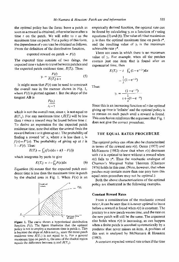
Fi ;ure 2. Change in the distribution of seed type v with time t spent trying to crack the seed. The curve labelled t = 0 shows the initial prior distribution of v corresponding to parameters c~ = 6 and fl = 5. The other two curves show the posterior distribution of v after times t = 2 and t=4.


sponds to the values a = 6 , f l= 5, and hence has mean p = 1 and standard deviation a=�89

Failure to open the seed gives the bird information about the likelihood of various values of v and in consequence the distribution of v can be updated. A particular example is given in Fig. 2. This shows that the distribution is both distorted and shifted to the right as time on the patch increases. Small values o f v become less likely and the mean increases. In general the mean value of v after time t is

/~(t) - f l + t (11) ~ - 1

which increases linearly with t (see the Appendix for details). Since we are dealing with exponential distributions, p(t) is also the mean further time required to crack the seed after time t spent trying.

We can illustrate the dependence on a by noting that

t #(t) = # + - - (12)

~ - 1

by equations (9) and (11). Consider first the limiting case when c~ is infinite. By equation (10), a is then zero and hence v = # for every seed in the environment. In this case time spent unsuccessfully trying to crack the seed does not alter our estimate of v. Equat ion (12) confirms this since/~(t) remains equal to # for all t when ~ = oo. When cr is non-zero the distribution of v changes with t, the rate of change being slow for small a and rapid for large a. This is again confirmed by equation (12); ~ decreases as a increases and hence #(t) changes more rapidly with t. Intuitively small a mean there is little uncertainty in v and one is slow to revise one's estimate of it. As the initial uncertainty in v increases so does the rate at which one is prepared to change one's estimate of it.

The increase in the estimate of v with time is reflected in a decrease in the rate r(t). Let x denote the time taken to open a randomly-chosen seed. As shown in the Appendix, the density function and distribution function are given by the following equations:

t -(c~+ 1) f(t) = fi(1 + ~ )

1 t 1--F(t) = ( + ~ ) -

Thus, from equation (4)

= ~ 1 + ~ ) - I r(t) ~(

- f l + t

This shows that r(t) tends to zero as t increases. In particular r(t) will eventually fall below y* and it will become optimal to abandon the present seed and search for another one. It can also be seen that the rate at which r(t) decreases with t increases with ~r for given/~.

Table II gives some values of t* and y*. All entries in this table correspond to values of fl equal to c t -1 and hence are for p = 1. As one would expect from the above remarks t* decreases as a increases.

The time t gives information on the seed type v. I f we ignore this information and continue with every seed until if it cracked the resulting mean reward rate will by ~ = (z +/~)-1. This equals the value of ~* achieved when a = 0. Thus Table II shows the value of ~ for the case /~=1. It can be seen that the difference between y* and ~ increases with increasing a. This is as one might expect: information on v is most useful when v is highly variable. Note that y * - ~ also increases with decreasing z.

D I S C U S S I O N

By considering some simple examples, we have tried to illustrate the role of information in optimal foraging. The examples show that the reward rate on the patch must be based on what is expected to happen in the immediate future. The stochastic reward rate r that we use is analogous to the

Table II. Optimum maximum time on patch t* and reward rate y* when expected time to open a seed is 1 t

z t* y* ~ o

0"5 oo 0.6667 ~ 0 9"9996 0-6667 18 0'25 3.9454 0-6707 6 0.5 2.2818 0-7006 3 1 1.6180 0-7639 2 oo

1.0 oo 0.5000 oo 0 19.0000 0-5000 18 0.25 6-9874 0-5005 6 0"5 3.8845 0-5098 3 1 2.7321 0.5359 2 oo

2.0 oo 0-3333 oo 0 37.0000 0-3333 18 0.25 12.9983 0-3334 6 0.5 6.9501 0.3352 3 1 4.8284 0-3431 2

"[" i.e. f l = ~ - I.

McNamara & Houston:

age-specific mortality in life-history theory (see, for example, Charlesworth 1980). Both functions are concerned with the probability of an event happen- ing at a certain time, given that it has not occurred up to that time.

As Zach (1979) and Fitzpatrick (1981) realized, if r does not decrease then it is never optimal to leave before a reward is found. By incorporating some variation in the patch quality, it is possible to convert a constant r into a decreasing one. In one of our examples some of the patches are empty, in the other the patches vary in the time required to obtain the prey. The common feature is that, as the animal spends time on the patch without obtaining a prey item, it obtains information about the patch. This information can make it optimal for the animal to leave a patch before a prey item is found. The example based on cracking a seed illustrates that information is easier to acquire when there is a lot of variability in patch type.

We have phrased our analysis in terms of patches, but the concept of a patch is a very general one. The case of some patches being empty can be applied to the problem of deciding whether or not a female i s receptive (Parker 1974), i.e. each patch is a female and the male has to decide how long to spend courting a female before deciding that she is unreceptive and giving up.

Similarly, the case where some patches are harder than others can be applied to problems that appear very different from that of a bird cracking a seed. For example, a predator such as a lion may gain information during a chase about the probability that the chase will be successful and so abandon a chase if the probability is too low. The impor- tance of variance in prey ability for the success of lion attacks is discussed by Elliott et al. (1977).

As we have already mentioned, our analysis is relevant to the decisions of foragers that wait at various sites ('patches') for prey to appear. Such predators must decide how long to wait for a prey item before moving on to another, possibly better, site. In the case of predators such as kingfishers and kestrels the disturbance that results from the capture of a prey item probably severely reduces the subsequent encounter rate with prey at the site, so that a site effectively contains just one item. This is not necessarily so in the case of the spotted flycatcher (Muscicapa striata), which may take many prey while operating from the same perch (Davies 1977).

In the cause of clarity we have kept our examples as simple as possible. One major simplification is that patches never contain more than one item. As

Patch use and information 559

a result it is always optimal to leave once an item has been found. The time on a patch is thus either the time to find an item or what we have called the maximum time on patch. The latter is the time at which the animal gives up, but we have refrained from referring to it as the giving-up time. We feel that the giving-up time (reviewed and analysed by McNair 1982) is the time between the capture of an item and the departure from the patch. In our examples the giving-up time in this sense is zero, but the animal can conveniently be thought of as not being prepared to spend longer than a certain amount of time in the patch. (Note that the giving-up time does not limit the patch residence time in a simple way.) Problems involving more than one item per patc h are difficult but some progress has been made in analysing them (Green, 1980, 1984; Iwasa et al. 1981; McNair 1982; McNamara 1982).

Another important simplification is that the only information available to the animal is the time that it has spent in the patch. It is reasonable to suppose, however, that there will be other indications of patch type that can be used. As Fitzpatrick (1981) mentions in his discussion of the foraging behaviour of South American flycatchers, foraging sites differ in the time required to search them, and the bird may adjust its behaviour accordingly.

Although it would be possible to incorporate these complicating factors into our model we feel that this would obscure the general effects we have attempted to illustrate. Furthermore, since the simple model itself provides a good representation of many foraging problems, we hope that our detailed analysis of it will be of use to other workers in this area.

A P P E N D I X

Assume that the time taken to crack a nut of type v is exponential with mean v, and that v has prior density function

h(v; (~,/~) = ~ v (~ fl/v

Then

v>O (AI.1)

(A1.2)

F(~) fl~-I ~ - 1

This is also the mean time to crack a randomly- selected nut since E(X)= E{E(XIv)} and E(XIv)= v.


Similarly one can evaluate E(v 2) and hence

deduce that 8 2

Var v = (~ - 1)2(~ _ 2 )

After time t spent unsuccessfully trying to crack a nut the posterior density for v is proport ional to the product o f the prior and the likelihood P(X> tlv); i.e. proport ional to (as a function of v)

v-(~+ Oe -~lv x e -t/~ = v-(~+i)e-(~ +0/~

It follows immediately that v has posterior density h(v; a,fl+t). In particular, by equat ion (A1.2) and the 'lack of memory' property o f the exponential distribution, the expected further time needed to crack the nut is

p + t

The distribution function of X can be found as follows.

P(X> t) = E{p(X> t/v)}

= f~Ffl--~) v-(~+Oe-~/~e-t/~dv

~ r(~) = (1 + t / f l ) ~

F(~) (fl + t) ~ Thus

1 - F ( x ) = (1 + , / / ~ ) - "

Differentiating we obtain

f ( x ) = ~(1 + t/r) -(~+ 1l

Finally, by equation (3) and a simple integration

Thus, by equation (2)

1 - - Z c~

where z = (1 + t/B)-1

ACKNOWLEDGMENTS

REFERENCES

Charlesworth, B. 1980. Evolution in Age-structured Popu- lations. Cambridge: Cambridge University Press.

Charnov, E. L. 1976. Optimal foraging: the marginal value theorem. Theor. Pop. Biol., 9, 129-136.

Davies, N. B. 1977. Prey selection and the search strategy of the spotted flycatcher (Museicapa striata), a field study on optimal foraging. Anita. Behav., 25, 1016-1033.

Elliott, J. P., Cowan, I. MeT. & Holling, C. S. 1977. Prey capture by the African lion. Can. J. Zool., 55, 1811-1828.

Fitzpatrick, J. W. 1981. Search strategies of tyrant flycatchers. Anim. Behav., 29, 810-821.

Green, R. F. 1980. Bayesian birds: a simple example of Oaten's stochastic model of optimal foraging. Theor. Pop. Biol., 18, 244-256.

Green, R. F. 1984. Stopping rules for optimal foragers. Am. Nat., 123, 30-40.

Greig-Smith, P. In press. Statistical problems in the study of seed-eating birds. In: Statistics in Ornithology (Ed. by B. J. T. Morgan & P. M. North). Berlin: Springer- Verlag.

Iwasa, Y., Higashi, M. & Yamamura, N. 1981. Prey distribution as a factor determining the choice of optimal foraging policy. Am. Nat., 117, 710-723.

Johns, M. & Miller, R. G. 1963. Average renewal loss rate. Ann. Math. Stat., 34, 396-401.

Kamil, A. C. 1983. Optimal foraging theory and the psychology of learning. Am. Zool., 23, 291-302.

McNair, J. N. 1982. Optimal giving-up times and the marginal value theorem. Am. Nat., 119, 511-529.

McNamara, J. M. 1982. Optimal patch use in a stochastic environment. Theor. Pop. Biol., 21, 269-288.

McNamara, J. M. & Houston, A. L 1980. The application of statistical decision theory to animal behaviour. J. theor. Biol., 85, 673-690.

McNamara, J. M. & Houston, A. I. 1983. Optimal responding on variable interval schedules. Behav. Anal. Letters, 3, 157-170.

Oaten, A. 1977. Optimal foraging in patches: a case tbr stochasticity. Theor. Pop. Biol., 12, 263-285.

Parker, G. A. 1974. Courtship persistence and female- guarding as male time investment strategies. Behaviour, 48, 157 184.

Pietrewicz, A. T. & Kamil, A. C. 1981. Search images and the detection of cryptic prey: an operant approach. In: Mechanisms of Optimal Foraging (Ed. by A. C. Kamil & T. D. Sargeant), pp. 3I 1-331. New York: Garland Press.

Zach, R. 1979. Shelldropping: decision-making and optimal foraging in northwestern crows. Behaviour, 68, 106-117.

This work was motivated by discussions with Al Kamil and John Krebs. A.I.H. was supported by an SERC grant to Dr N. B. Davies.

(Received 30 August 1983; revised 4 April 1984; MS. number: 2434)

a simple model of information use in the exploitation of patchily distributed food

Documents