1

A Simple Heuristic for Reducing the Number of Scenarios in Two-stage Stochastic Programming

Ramkumar Karuppiah, Mariano Martin, and Ignacio E. Grossmann*

Department of Chemical Engineering, Carnegie Mellon University, Pittsburgh, PA

15213, U.S.A.

ABSTRACT

In this work we address the problem of solving multiscenario optimization models

that are deterministic equivalents of two-stage stochastic programs. We present a

heuristic approximation strategy where we reduce the number of scenarios and obtain an

approximation of the original multiscenario optimization problem. In this strategy, a

subset of the given set of scenarios is selected based on a proposed criterion and

probabilities are assigned to the occurrence of the reduced set of scenarios. The original

stochastic programming model is converted into a deterministic equivalent using the

reduced set of scenarios. A mixed-integer linear program (MILP) is proposed for the

reduced scenario selection. We apply this practical heuristic strategy to four numerical

examples and show that reformulating and solving the stochastic program with the

reduced set of scenarios yields an objective value close to the optimum of the original

multiscenario problem.

Keywords: Two-stage stochastic programming; Multiscenario model; Scenario

reduction; Approximation

* Corresponding author. Tel.: +1-412-268-3642; fax: +1-412-268-7139.

Email address: grossmann@cmu.edu (I.E. Grossmann)

2

1. INTRODUCTION

Optimization under uncertainty is a major issue in solving real world problems.

Uncertainty is a common feature that presents itself during the operation or design of any

system. There is an abundance of literature in the area of optimization under uncertainty

involving several applications. Some of these include: production planning (Clay and

Grossmann, 1997; Cheng et al., 2003), scheduling (Birge and Dempster, 1996;

Balasubramanian and Grossmann, 2002), optimal chemical process synthesis (Acevedo

and Pistikopoulos, 1998; Liu and Sahinidis, 1996; Rooney and Biegler, 2003), electricity

production (Takriti et al., 1996; Nowak et al., 2005). Usually problems with uncertainty

are represented as stochastic programming problems (Birge and Louveaux, 1997) or as

deterministic flexibility problems (Grossmann et al., 1983). The focus of this work is on

solving two-stage stochastic programs with recourse, where we have some uncertain

parameters that either follow a continuous distribution or take on a finite set of values.

The aim in such problems is to determine the 1st stage decision variables such that the

sum of the 1st stage costs and the expected value of the 2nd stage costs is minimized.

Other approaches for solving problems under uncertainty include robust optimization,

probabilistic programming, fuzzy optimization, and dynamic programming. Sahinidis

(2004) presents a recent review of problems under uncertainty along with the approaches

used to solve such problems.

Algorithms for stochastic integer programs have been presented by Ahmed et al.

(2004), Carøe and Tind (1997), Carøe and Schultz (1999), Klein Haneveld et al. (1995,

1996) among other authors. Norkin et al. (1998) have developed a branch and bound

technique for global optimization of nonconvex nonlinear stochastic programs, where

stochastic lower and upper bounds are made to converge with some confidence levels. In

two-stage stochastic programming with recourse, a common approach is to discretize the

uncertain parameter space and formulate a deterministic equivalent of the stochastic

program, which leads to a multiscenario optimization problem (Dantzig, 1963). A single

combination of the values of the uncertain parameters leads to a particular scenario. In

this discretization approach there are usually a number of uncertain parameters in a

3

system and these are assumed to take on a finite set of values. All possible combinations

of these values lead to an explosion in the number of scenarios. This greatly increases the

size of the optimization problem, making it very hard to solve. To overcome this

problem, approximation methods have been developed to solve the stochastic program

with fewer scenarios and still obtain a close to optimal solution. Novak and Kravanja

(1999) have presented a reduced dimensional stochastic optimization technique where

they determine a subset of the vertices of the feasible polyhedral space of the uncertain

parameters and their corresponding weights to approximate the expected value of the

objective function of the original problem. Dupačová et al. (2003) have also proposed a

scenario reduction technique based on a different probability metric. Sampling methods

(e.g. Monte Carlo sampling) are also quite attractive to convert the continuous space of

uncertain parameters into a smaller discrete space. Sample Average Approximation

(SAA) has also been used to solve stochastic mixed-integer nonlinear programs (for

example see Wei and Realff, 2002).

In this work we address the problem of reducing the number of scenarios in

multiscenario optimization problems. We use a similar idea as given in Novak and

Kravanja (1999), and Dupačová et al. (2003) to select a subset of scenarios from a given

larger set for solving the stochastic program. The goal is that the optimal objective of the

full scenario problem is closely approximated by the optimal objective value of the

reduced problem. A mixed-integer linear programming (MILP) model is presented for the

selection of the subset of scenarios. The remainder of the paper is organized as follows.

Section 2 presents the problem statement, while the heuristic strategy to approximate the

original multiscenario problem is given in Section 3. Numerical examples on which the

approach was applied are given in Section 4, and finally Section 5 summarizes the

conclusions.

2. PROBLEM STATEMENT

We are given a two-stage stochastic program whose deterministic equivalent has

S separate scenarios with different realizations of uncertain parameters. Each of these

4

scenarios has a certain probability of occurrence. The uncertain parameters that make up

these scenarios take on a finite set of values. The probabilities of this finite set of values

for each uncertain parameter add up to 1. This discrete finite set is either given, or else it

can be computed from a continuous distribution (see Luceno, 1999).

The goal of this paper is to develop an approach where we can select a subset S ′

of scenarios from the original set of scenarios ( S ) with new probabilities given to each of

the S ′ scenarios, and approximate the optimal objective value of original multiscenario

problem as closely as possible with the reduced number of scenarios. This means that on

solving the reduced dimensional problem (with fewer scenarios), we get an objective

value close to one of the original multiscenario problem with S scenarios. The problem

at hand is to devise an MILP (or a linear programming (LP)) formulation that allows us to

select a subset of the scenarios, and gives us their associated probabilities that would help

in approximating the original optimization problem. We are also interested in getting

some bounds on the theoretical error estimates.

3. APPROXIMATION STRATEGY

Two-stage stochastic programs are often converted to deterministic multiscenario

optimization problems, by discretizing the uncertain parameters in a finite set of

scenarios. Such problems grow larger with the number of scenarios. A multiscenario

model with a scenario set S can be expressed as follows:

Θ∈∈∈

∈⎪⎭

⎪⎬⎫

≤

=

+= ∑

ss

sss

sss

sssss

xd

XxDd

Ssxdg

xdhts

xfpdfzs

θ

θ

θ

θ

,,

0),,(

0),,(..

),()(min 0

,

(P)

where Ss ∈ is a single scenario in the multiscenario problem. d is the set of 1st stage

decision variables, while sx is the set of 2nd stage variables in scenario s. sθ is the vector

of uncertain parameters in scenario s. 0(.) =h and 0(.) ≤g include the first and second

stage constraints. Our goal is to approximate the set with S scenarios with a set with S ′

5

scenarios so that we have a smaller multiscenario problem that yields close to optimal

expected objective value.

3.1 Selection of subset of scenarios

In a multiscenario problem let { } Iii ,,1K== θθ be the vector of uncertain parameters.

Let the uncertain parameter iθ take on a finite set of values given by { }ii

iJj

ji ,,1K=θ . The

probability associated with the uncertain parameter iθ taking on a value ijiθ is ij

ip . With

multiple uncertain parameters, these can be combined together by considering the

corresponding Cartesian product of all the values of the uncertain parameters to yield the

set with S scenarios. The scenario s involves the following vector of uncertain

parameters { } Iij

isi

,,1K== θθ , and there are a total of ∏=

=I

iiJS

1

scenarios. Assuming

independent distributions, the probability associated with a scenario s in the original set

of scenarios is given by ∏=

==I

i

jiIjjjs

iI

ppp1

,,2,1 21 K .

In order to select a minimum subset from the original set of scenarios, we propose

the following heuristic criterion:

Criterion: The sum of the probabilities of the new scenarios in which the uncertain

parameter value ijiθ appears is equal to ij

ip .

The above criterion should hold for all of the values of each of the uncertain

parameters. Furthermore, the sum of the probabilities of the reduced set of scenarios

should be equal to 1. We want to re-arrange the scenario probabilities in such a way that

the overall probability of occurrence of a particular value of an uncertain parameter

across different scenarios matches the probability of occurrence of that value for the

given uncertain parameter. The motivation behind such an approximation is to

heuristically reduce the approximation error. If the objective function of a multiscenario

optimization formulation can be approximated as a sum of the functions of the individual

uncertain parameter values multiplied by the respective probabilities of the scenarios in

6

which they occur its value will be close to ∑∑∑ ∑= ==

=I

i

J

j

jii

ji

s

I

i

siis

i

i

ii fpfp1 11

)(.)(. θθ . The re-

assignment of probabilities to selected scenarios based on the above-mentioned criterion

and solving the optimization problem will then give an objective function that can be

approximated by ∑∑∑ ∑= =′ =

′′ =

I

i

J

j

jii

ji

s

I

i

siis

i

i

ii fpfp1 11

)(.)(. θθ . Since the objective functions of the

original and the reduced scenario problem can be approximated by the same expression,

the difference between their values is also expected to be small.

To illustrate the scenario reduction approach with a small example, consider two

uncertain parameters 1θ , and 2θ , where each parameter can take on two values. Let 1θ

take the two values {2,5} each occurring with a probability of 0.5, and let parameter 2θ

take a value of 30 with a probability of 0.5 and a value of 70 with a probability of 0.5.

We obtain a set of four scenarios {(2,30), (2,70), (5,30), (5,70)} that result from the

Cartesian product of {2,5} and {30,70}. These are shown in Fig. 1 and denoted by (1),

(2), (3) and (4). The probability of occurrence of each of these scenarios is 0.25, which is

obtained by multiplying the probabilities of the uncertain parameter values in each

scenario.

Fig. 1 Scenarios in illustrative example

Looking at the 1θ axis, we find that 1θ takes a value of 2 in scenarios (1) and (4),

where each of these scenarios occurs with a probability of 0.25, thus making the overall

1θ

2θ

2 5

70

30(1)

(3)

(2)

(4)

p=0.25 p=0.25

p=0.25 p=0.25

7

probability of occurrence of the value 2 for 1θ to be 0.5. The creation of scenarios has

separated the value of 2 taken by 1θ into different scenarios. However, the creation of

scenarios has ensured that the sum of the probabilities of the scenarios in which 1θ takes

a value of 2 is the same as the occurrence probability of 1θ =2, which is 0.5. The same

analysis is true for the value of 5 taken on by 1θ . When looking at the 2θ axis, we can

find an identical analysis for the values taken on by 2θ .

To reduce the number of scenarios, we use the idea of reversing this

disaggregation of uncertain parameter values and their probabilities, and combining back

the scenarios so that the probabilities of occurrence of the individual uncertain parameter

values remain intact. One possible re-combination is shown in Fig. 2a, where scenario (2)

is combined with scenario (1), while scenario (4) is combined with scenario (3), leading

to the new scenarios (1’) and (3’) in Fig. 2b.

Fig. 2a Re-combination of scenarios in illustrative example

1θ

2θ

2 5

70

30(1)

(3)

(2)

(4)

p=0.25 p=0.25

p=0.25 p=0.25

8

Fig. 2b Scenarios with modified probabilities in illustrative example

In Fig. 2b, the individual uncertain parameter values have the same probability of

occurrence through the scenarios (1’) and (3’), as when the scenarios had not even been

created. For instance, looking at the 1θ axis, we see that 1θ takes a value of 2 only in

scenario (1’), which has a probability of 0.5 ensuring the probability of occurrence of the

value 2 for 1θ to be 0.5. Similarly for 1θ =5, this value now occurs only in scenario (3’)

whose probability is 0.5, meaning that 1θ =5 occurs with a probability of 0.5 in the

overall system, which is the probability of occurrence of the value 5 for 1θ . A similar

analysis holds for the values on the 2θ axis.

The minimum number of reduced scenarios that we can obtain depends also on

the individual probabilities of the values taken on by the uncertain parameters. To

illustrate this, let 1θ now take two values {2,5} each occurring with corresponding

probabilities of 0.3 and 0.7, respectively. The parameter 2θ takes a value of 30 with a

probability of 0.6 and a value of 70 with a probability of 0.4. Combining these two

uncertain parameters, we obtain four scenarios as shown in Table 1.

1θ

2θ

2 5

70

30(1’)

(3’)

p’=0.50

p’=0.50

9

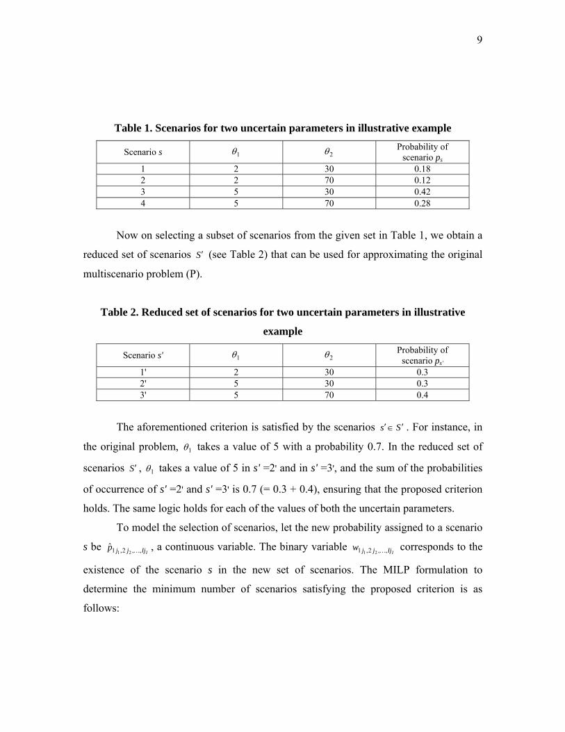
Table 1. Scenarios for two uncertain parameters in illustrative example

Scenario s 1θ 2θ Probability of scenario ps

1 2 30 0.18 2 2 70 0.12 3 5 30 0.42 4 5 70 0.28

Now on selecting a subset of scenarios from the given set in Table 1, we obtain a

reduced set of scenarios S ′ (see Table 2) that can be used for approximating the original

multiscenario problem (P).

Table 2. Reduced set of scenarios for two uncertain parameters in illustrative

example

Scenario s' 1θ 2θ Probability of scenario ps'

1' 2 30 0.3 2' 5 30 0.3 3' 5 70 0.4

The aforementioned criterion is satisfied by the scenarios Ss ′∈′ . For instance, in

the original problem, 1θ takes a value of 5 with a probability 0.7. In the reduced set of

scenarios S ′ , 1θ takes a value of 5 in s' =2' and in s' =3', and the sum of the probabilities

of occurrence of s' =2' and s' =3' is 0.7 (= 0.3 + 0.4), ensuring that the proposed criterion

holds. The same logic holds for each of the values of both the uncertain parameters.

To model the selection of scenarios, let the new probability assigned to a scenario

s be IIjjjp ,,2,1 21

ˆ K , a continuous variable. The binary variable IIjjjw ,,2,1 21 K corresponds to the

existence of the scenario s in the new set of scenarios. The MILP formulation to

determine the minimum number of scenarios satisfying the proposed criterion is as

follows:

10

{ } IIjjj

IIjjj

IIjjjIjjj

J

jIjjj

J

j

J

j

IIj

I

J

jIjjj

J

j

J

j

jJ

jIjjj

J

j

J

j

jJ

jIjjj

J

j

J

j

J

jIjjj

J

j

J

j

jjjw

jjjp

jjjwp

p

Jjpp

Jjpp

Jjpp

ts

wf

I

I

II

I

I

I

II

I

I

I

I

I

I

I

I

I

I

I

,,,1,0

,,,1ˆ0

,,,ˆ

1ˆ

,,1ˆ

,,1ˆ

,,1ˆ

..

min

21,,2,1

21,,2,1

21,,2,1,,2,1

1,,2,1

1 1

1,,2,1

1 1

2221

,,2,11 1

1111

,,2,11 1

1,,2,1

1 1

21

21

2121

21

1

1

2

2

1

1

21

1

1

2

2

221

1

1

3

3

121

2

2

3

3

21

1

1

2

2

K

K

K

K

KK

M

KK

KK

K

K

K

KK

K

K

K

K

K

∀∈

∀≤≤

∀≤

=

==

==

==

=

∑∑ ∑

∑∑ ∑

∑∑ ∑

∑∑ ∑

∑∑ ∑

== =

== =

== =

== =

== =

−

−

(SG)

On solving the MILP model (SG) we obtain the minimum set of scenarios and

their associated probabilities. The numerical value of the probability corresponding to a

scenario s with the uncertain parameters { }IjI

jj θθθ ,,, 2121 K in the reduced set of scenarios is

*,,2,1 21

ˆIIjjjp K .

Remarks

1. Since the problem (SG) yields a very large MILP problem, we can consider

instead a linear programming relaxation (SG-L) to obtain a set of scenarios

satisfying the proposed criterion. This can be done by eliminating the binary

variables and modifying the objective function as given in the formulation below:

11

IIjjj

J

jIjjj

J

j

J

j

IIjI

J

jIjjj

J

j

J

j

jJ

jIjjj

J

j

J

j

jJ

jIjjj

J

j

J

j

J

jIjjj

jI

jjJ

j

J

j

jjjp

p

Jjpp

Jjpp

Jjpp

ts

ppppf

I

I

I

I

II

I

I

I

I

I

I

I

I

I

I

I

I

,,,1ˆ0

1ˆ

,,1ˆ

,,1ˆ

,,1ˆ

..

ˆ).1(min

21,,2,1

1,,2,1

1 1

1,,2,1

1 1

2221

,,2,11 1

1111

,,2,11 1

1,,2,121

1 1

21

21

1

1

2

2

1

1

21

1

1

2

2

2

21

1

1

3

3

1

21

2

2

3

3

21

211

1

2

2

K

K

KK

M

KK

KK

KK

K

K

K

K

K

K

∀≤≤

=

==

==

==

−=

∑∑∑

∑∑∑

∑∑∑

∑∑∑

∑∑∑

== =

== =

== =

== =

== =

−

−

(SG-L)

The weights in the new objective function involve the known probabilities of the

existing set of scenarios and are present to drive the optimization to reduce the

number of scenarios while trying to keep the original set of scenarios that had

relatively larger probabilities. The solution will be a subset of the initial set of S

scenarios, although it is not guaranteed to be the minimum number of scenarios

since the problems (SG) and (SG-L) are not equivalent.

2. It is also possible to assign weights to the individual terms in (SG) to help select

scenarios with new probabilities close to their original probabilities.

3. In this method for determining a smaller number of scenarios, it may be possible

to identify the worst-case scenarios from among the given discrete set of scenarios

(that guarantee feasibility of design for all the given discrete scenarios). If such

scenarios exist, and are easily identified, they can be included in the reduced set

of scenarios. In the MILP formulation (SG), this would mean assigning a lower

bound on the probability of the worst-case scenarios (if known) as

12

ε≥− scenarioscaseworstp where ε is a small positive number less than or equal to 1. The

binary variables scenarioscaseworstw − are also fixed to a value of 1.

4. The theoretical minimum number of scenarios that can be obtained using this

method is the maximum of the number of independent values that each uncertain

parameter can take. The other limiting case is that if no value of an uncertain

parameter occurs in more than a single scenario in the set S, the number of

scenarios cannot be reduced with this method.

3.2 Reduced scenario optimization

The stochastic optimization problem (P') that uses a reduced set of scenarios S ′ is

as follows:

Θ∈∈∈

′∈′⎪⎭

⎪⎬⎫

≤

=

+=′

′′

′′′

′′′

′′′′′∑

′

ss

sss

sss

sssss

xd

XxDd

Ssxdgxdh

ts

xfpdfzs

θ

θ

θ

θ

,,

0),,(0),,(

..

),()(min 0

,

(P')

All the functions in (P') have the exact same form as the corresponding functions

in (P). sp ′ is the probability of a selected scenario s′ obtained by solving (SG) or (SG-L).

The optimal value of the design variable vector obtained by solving (P') is denoted by d ,

and the optimal expected objective value by *z ′ . In case the worst-case scenarios from

the set S are included in the set S ′ , then d will be feasible for every scenario in the

original scenario set S (Grossmann et al., 1983). We can also solve the original problem

(P) by fixing the design variables in (P) to the value d . Note that this makes the model

(P) decomposable into S separate optimization subproblems with each subproblem

corresponding to a single scenario. Solving (P) by fixing the design variables to the value

d gives us a locally optimal solution to the original problem where the optimal objective

value obtained using this method is *~z .

13

For practical purposes, we can obtain a bound on the error in such an

approximation as follows:

(a) The expected objective value is computed by solving each scenario (SPs)

separately (e.g. wait-and-see approach) or may be approximated by taking a subset of

scenarios with larger probabilities. The optimal objective values of all considered

scenarios Ss ∈ are summed to obtain ∑=s

sB zz ** .

(b) The objective value of the best found feasible solution so far is *~z (this value is

either the global minimum or higher than it). The value of **~ BzzEB −= is calculated,

which is an upper bound on the error using the approximation technique. Note that this

bound may be loose.

4. NUMERICAL EXAMPLES

The proposed scenario reduction and approximation approach is applied to four

examples. The optimization problems are formulated using GAMS (Brooke et al., 1998)

and solved on an Intel Pentium IV Windows machine with 512 MB memory. The LP and

MILP problems are solved using GAMS/CPLEX 9.0 while GAMS/ CONOPT 3.0 is used

for the nonlinear programming (NLP) problems.

Example 1 This small example is taken from Clay and Grossmann (1997) and

corresponds to problem (EX1) in that paper. It is a stochastic program with 2 uncertain

parameters { }21,θθ and one 1st stage decision variable (d). In order to convert this problem

into its deterministic equivalent, the uncertain parameters are assigned three values each,

which leads to the creation of the LP deterministic equivalent with 9 scenarios. The two

uncertain parameters are given by 1θ and 2θ , each with 3 values and associated

probabilities as follows:

}2.0,6.0,2.0{},2,5.1,1{ 1111 == jj pθ

}2.0,7.0,1.0{},2,5.1,1{ 2212 == jj pθ

The LP deterministic equivalent is as follows:

14

3,,1,3,,1,

3,,1,3,,1

3,,1,3,,12

3,,1,3,,13..

)(min

211

21

1

1

212121

21212

21211

3

1

3

1212,1

2121

21

2121

21

21

21

21

1 2

212121

KK

KK

KK

KK

==ℜ∈ℜ∈

ℜ∈

==+≤−+

==+−≥

==−≥

++=

++

+

= =∑∑

jjxx

d

jjdxx

jjx

jjxts

xxpdz

jjjj

jjjjjj

jjjj

jjjj

j jjjjjjj

θθ

θθ

θθ

(E1)

In the above formulation, 211 jjx and

212 jjx are the continuous 2nd stage variables

and 2121 212,1 . jj

jj ppp = .

The LP formulation for the deterministic equivalent (E1) with 9 scenarios has 19

continuous variables and 27 constraints. Solving this model yields an optimal objective

value of 10.1, where the optimal value of the 1st stage variables is 4.0. We apply the

scenario reduction technique to this problem and obtain the 4 scenarios in Table 3.

Table 3. Reduced number of scenarios for example 1

Scenario s' 1θ 2θ Probability of scenario ps'

1' 1 1 0.1 2' 1.5 1.5 0.6 3' 2 2 0.2 4' 1 1.5 0.1

The corresponding reduced LP problem has 4 scenarios, 9 continuous variables

and 12 constraints. It is to be noted that an inspection of the values of the uncertain

parameters and their corresponding probabilities is used in determining the reduced set of

scenarios, such that the criterion given in Section 3.1 is satisfied. The MILP formulation

(SG) is not used to select the scenarios in this example. On solving the reduced scenario

problem, we obtain the optimum value of 10.1, and the value of the 1st stage variable is

again 4.0. This means that we have a zero approximation error in this case. Note however

that the reduced set of scenarios is not unique. Solving the model (P') with different

scenarios with different probabilities could potentially lead to a value of the design

variable that is infeasible for the original problem (P). A design variable obtained by

15

solving the approximate model (P') will be feasible for the original problem only if the

worst-case scenarios from the original set of 9 scenarios are included in the reduced set of

scenarios used in formulating (P').

Example 2 We solve the model (EX2P) taken from Clay and Grossmann (1997) as a next

example. This is an LP with 10 continuous variables and 18 constraints. It has 2 uncertain

parameters that are assumed to take on 3 values, each leading to a total of 9 scenarios.

The two uncertain parameters and their distributions are given below:

}3.0,5.0,2.0{},3,2,1{ 1111 == jj pθ

}2.0,6.0,2.0{},3,2,1{ 2222 == jj pθ

The formulation corresponding to this example is as follows,

3,,1,3,,1

3,,1,3,,12

3,,1,3,,1..

.min

211

2

1

2122

2112

3

1

3

122,1

21

2

21

1

21

1 2

2121

KK

KK

KK

==ℜ∈

ℜ∈

==≥+

==≥+

+=

+

+

= =∑∑

jjxd

jjxd

jjxdts

xpdz

jj

jjj

jjj

j jjjjj

θ

θ

(E2)

where d and 212 jjx are the continuous 1st and 2nd stage variables, respectively, and the

probability 2121 212,1 . jj

jj ppp = .

Solving this model, we obtain an optimum expected value of 1.6333, and the

optimal value of the 1st stage variable is 0.6667. Using the proposed scenario selection

approach, we can obtain a minimum of 4 scenarios satisfying the proposed probability

criterion in Section 3.1. The formulation (SG) corresponding to this example is given

below,

16

{ } 3,,1,3,,11,0

3,,1,3,,11ˆ0

3,,1,3,,1ˆ

1ˆ

2.0ˆˆˆ6.0ˆˆˆ2.0ˆˆˆ3.0ˆˆˆ5.0ˆˆˆ2.0ˆˆˆ

..

min

212,1

212,1

212,12,1

3

1

3

12,1

23,1323,1223,11

22,1322,1222,11

21,1321,1221,11

23,1322,1321,13

23,1222,1221,12

23,1122,1121,11

3

1

3

12,1

21

21

2121

1 2

21

1 2

21

KK

KK

KK

==∈

==≤≤

==≤

=

=++

=++

=++

=++

=++

=++

=

∑ ∑

∑ ∑

= =

= =

jjw

jjp

jjwp

p

ppp

ppp

ppp

ppp

pppppp

ts

wf

jj

jj

jjjj

j jjj

j jjj

(SG-E2)

Table 4 shows the scenarios obtained by solving the above formulation (SG-E2).

Table 4. Reduced number of scenarios for example 2 obtained from solving

model (SG-E2)

Scenario s' 1θ 2θ Probability of scenario ps'

1' 1 3 0.2 2' 2 2 0.5 3' 3 1 0.2 4' 3 2 0.1

On solving the reduced dimensional model (P') with the four scenarios shown in

Table 4 obtained by solving model (SG-E2), we obtain an optimal value of *z′ = 1.6833,

and the optimal value of the design variable is found to be 0.667. Fixing the value of the

design variable d to 0.667 in model (E2) and re-solving it we obtain the optimal objective

value of *~z = 1.6333 which is the same as the optimum of model (P). We also see if we

can refine the solution by generating the scenarios using model (SG-L). We find that we

obtain the same set of 4 scenarios, as shown in Table 4, by solving (SG-L) corresponding

to this example.

17

Example 3 The third example is a larger case study and is taken from Novak and

Kravanja (1999) with some modifications. This problem corresponds to the design of a

heat exchanger network with 5 heat exchangers, 2 hot streams, 2 cold streams, and 2

utilities. The network structure is given is Fig. 3.

Fig. 3 Heat exchanger network for example 3

The three temperatures T3, T5 and T9 are uncertain parameters that change during network

operation. Each of these uncertain parameters is assumed to take on 5 values with

probabilities )( p given in Table 5.

Table 5 Values and probabilities for uncertain parameters T3, T5, T9

j jT3 (°C) )( 3

jTp jT5 (°C) )( 5jTp jT9 (°C) )( 9

jTp 1 378.9 0.007 573.9 0.007 293.5 0.007 2 382.6 0.1545 577.6 0.1545 295.3 0.1545 3 388.0 0.677 583.0 0.677 298.0 0.677 4 393.4 0.1545 588.4 0.1545 300.7 0.1545 5 397.1 0.007 592.1 0.007 302.5 0.007

The optimization problem is formulated as a two-stage stochastic program, which

is converted to its multiscenario equivalent. There are a total of 125 scenarios in this

problem. The goal of the design problem is to minimize the expected total cost that

includes the capital cost of the heat exchangers and the expected utility cost. The heat

18

exchanger areas are the 1st stage design variables, while the heat loads and the

temperatures that are not fixed are the 2nd stage variables. The multiscenario model (E3)

is as follows:

19

( ) ( )

( ) ( )

( ) ( )

( ) ( )

( ) ( )

rAKmWUKmWUUUU

s

rT

TTTTT

TTTT

TTTT

TT

T

TTTTTT

T

TTTT

T

TTTTTTTT

T

TTTTTT

T

rTU

A

TTTTT

TTT

TTTTTTT

ts

AApz

r

sr

s

ss

sss

s

sss

ss

ss

ss

s

ssss

sss

sss

ss

ssssss

sss

sssss

ss

srr

srr

ss

ss

sss

ss

sss

sssss

ssss

sss

rrs

∀≥=====

=

⎪⎪⎪⎪⎪⎪⎪⎪⎪⎪⎪⎪⎪⎪⎪⎪⎪⎪⎪⎪⎪⎪⎪

⎭

⎪⎪⎪⎪⎪⎪⎪⎪⎪⎪⎪⎪⎪⎪⎪⎪⎪⎪⎪⎪⎪⎪⎪

⎬

⎫

∀≥

≥

≤≤

−≤≤

≤≤

≤≤+

≤≤

≤≤+

−−−=⎟⎟⎠

⎞⎜⎜⎝

⎛

−−

Δ

−−−=⎟⎟⎠

⎞⎜⎜⎝

⎛

−−

Δ

−−−=⎟⎟⎠

⎞⎜⎜⎝

⎛

−−

Δ

−−−=⎟⎟⎠

⎞⎜⎜⎝

⎛

−−

Δ

−−−=⎟⎟⎠

⎞⎜⎜⎝

⎛

−−

Δ

=Δ

≥

+≥

−=

+=

−=

−=−=

−=−=

−=−=

⎥⎦

⎤⎢⎣

⎡⎟⎠

⎞⎜⎝

⎛+++= ∑ ∑

= =

0)/(1000),/(700

125,,1

00

3231

323314)1,394max(

6206201

619600620619

600620ln.

350350

ln.

313393313393

ln.

ln.

620620

ln.

5,,1

1)600(2000

6000/)350(1500

)313393(3000)(1000)(2000)(1000)(2000)620(1500

..

23.002.023501846min

25

24321

,

,1

,10,9

,5,8,3

,7

,5,6,3

,4,3

,2,3

,8,8

,5ln

,9,10,2,9

,10,2,4ln

,7,6,7

,6,3ln

,4,6,8,5,4,6

,8,5,2ln

,3,2,4,3,2

,4,1ln

,ln

,

,4,6

,8,5

,9,4,10

,2,4

,7,6,3

,4,8,6,5,2

,3,4,2,1

125

1,5,4

65.05

4

1

65.0

K

K

φ

φ

φφ

φφφφ

φφ

(E3)

20

In the above model, the subscript s corresponds to a particular scenario. sr ,φ

pertains to the heat load in heat exchanger r in scenario s. The 1st stage design variable rA

pertains to the area of heat exchanger r. T3,s , T5,s , T9,s are the values of the respective

uncertain parameters, T3, T5 and T9, in scenario s. The coefficient ps denotes the

probability of occurrence of scenario s, and is calculated by multiplying the individual

probabilities of the values of the uncertain parameters which occur in that scenario s. The

model (E3) with 125 scenarios is a nonconvex nonlinear program with 2,005 continuous

variables and 2,375 constraints. On solving this model, we obtain the optimal solution of

$45,223.07 with the following optimal values of the design variables:

A1 = 15.34 m2, A2 = 2.37 m2, A3 = 6.32 m2, A4 = 1.99 m2, A5 = 2.31 m2.

Applying our scenario reduction approach to this example, where we first solve

the MILP model (SG) for this problem, we obtain 5 scenarios (see Table 6).

Table 6. Reduced number of scenarios for example 3

Scenario s′ sT ′,3 (°C) sT ′,5 (°C) sT ′,9 (°C) sp ′

1' 378.9 573.9 293.5 0.007 2' 382.6 577.6 295.3 0.1545 3' 388.0 583.0 298.0 0.677 4' 393.4 588.4 300.7 0.1545 5' 397.1 592.1 302.5 0.007

On using the above 5 scenarios in problem (E3), reformulating it and solving it,

we obtain a nonconvex NLP model with 86 variables and 96 constraints. The optimal

objective of this reduced problem is $45,310.08, which is 0.2% higher that the optimum

of the original multiscenario problem with 125 scenarios. The optimal values of the

design variables so obtained are 1A = 15.28 m2, 2A = 2.43 m2, 3A = 6.38 m2, 4A = 1.98

m2, 5A = 2.31 m2. On solving the 125 scenario model (E3) by fixing the design variables

to the optimal values obtained by solving the reduced model, we obtain an expected cost

of *~z = $45,225.36 which is almost the exact solution of the original stochastic program.

In terms of the computational times for solving the optimization problems, it takes 20.2

CPU s to solve (E3), while the reduced dimensional problem with 5 scenarios is solved in

21

just 0.24 CPU s. On fixing the design variables (areas of heat exchangers) in the model

(E3), we are able to solve it in 9.8 CPU s to obtain *~z = $45,225.36.

Example 4 The last example is a modified version of the one used by Acevedo and

Pistikopoulos (1998) and Wei and Realff (2004). The original problem involves the

production of 5 products from 5 raw materials using 11 different processes (Fig. 4). In

this problem, the uncertain parameters are the maximum availabilities of raw materials,

and the demands for products. The continuous decision variables are the capacities for the

processes, whereas the binary variables denote the selection of the required processes.

Fig. 4 Process network for example 4

The deterministic model for this example is based on basic mass balances and is

described as follows.

22

In Fig. 4, the nodes are either splitters or mixers. ),( 1unitunitF is the mass flow rate from a source ‘unit’ to a destination ‘unit1’. For a splitter ‘split’ connected to a source ‘unit’ and destinations ‘unitq’, the mass balance is given by,

∑=q

qunitsplitFsplitunitF ),(),(

For a mixer ‘mix’, with input connections from ‘unitq’ and an output to ‘unit’, the mass balances are,

),(),( unitmixFmixunitFq

q =∑

A raw material j with flowrate ‘RMj’ is assumed to come from an inlet ‘sourcej’,

jRMunitsourceF jj ∀=),(

A product i with mass flow rate ‘Pi’ is assumed to go out to a destination ‘outi’,

iPoutunitF ii ∀=),(

The sum of the mass flows to a process k from inlet sources ‘unitq’ is equal to

‘ISk’,

kISprocessunitF kq

kq ∀=∑ ),(

The mass flow from a process k to a destination ‘unit’ is equal to ‘OSk’,

kISunitprocessF kk ∀=),(

Other balances include:

Yield relations kISPCOS kkk ∀=

Desired production iDP ii ∀≤

Availability of raw material jRMMaxRM jj ∀≤

Logic constraints kQMIIS kkk ∀≤− 0

kyQMaxQ kkk ∀≤− 0

The objective function is given by,

23

[ ]⎭⎬⎫

⎩⎨⎧

+−−−−= ∑∑∑∑====

11

1

11

1

5

1

5

1min

kkkkk

kkk

jjji

ii yFCQDCISOCRMPz αβ

The symbols in the previous equations are summarized as follows:

iD is the uncertain demand for product i (parameter)

kDC is cost for process k

),( 1unitunitF is the mass flow rate in the stream between unit and unit1

kFC is the fixed cost of process k (parameter)

kIS is the mass flow in input stream to process k (variable)

kQMax is the maximum volume capacity of process k (parameter)

jRMMax is the maximum availability of raw material j which is uncertain (parameter)

kMI is the mass flow to volume relationship constant for process k (parameter)

kOC is the operating cost of process k (parameter)

kOS is the mass flow in output stream to process k (variable)

iP is the mass flow of product i (variable)

kPC is the yield constant for process k (parameter)

kQ is the capacity of process k (variable)

jRM is the mass flow of raw material j (variable)

ky is the binary variable for selection of process k (binary variable)

jα is the cost of raw material j (parameter)

iβ is the price of product i (parameter)

Since iD and jRMMax are uncertain parameters, the above model is converted

into a two-stage stochastic program, which is then re-formulated as a deterministic

multiscenario model by discretizing the uncertain parameters. kQ and ky are the first

stage decision variables while the flows in the system, raw material consumptions, and

24

product flows are the second stage variables. The objective is to minimize the negative of

the profit function,

In the multiscenario formulation, the uncertain parameters are, 41, K=iDi , and

41, K=jRMMax j , and each of these is assumed to taken to two values. 5D and

5RMMax are assumed to be known and constant. The values for all the parameters used

in this example 4 can be seen in Table 7 where the two levels of the eight uncertain

parameters and their probabilities can also be found.

In this example we obtain an exact solution considering all the scenarios, and

compare that optimal value of the objective function with those obtained using the

proposed approach and by using Sample Average Approximation (SAA).

Table 7. Parameters used in the model for example 4 Process k 1 2 3 4 5 6 7 8 9 10 11 PCk 13 15 17 14 10 15 16 11 13 15 17 MIk 18 20 15 20 20 21 15 15 25 15 20 OCk 400 400 400 400 400 400 400 400 400 400 400 DCk 2500 2500 2500 2500 2500 2500 2500 2500 2500 2500 2500 FCk 400 2500 3500 300 4500 2500 300 2200 2800 2700 2500 Max Qk 3.0 3.0 3.0 3.0 3.0 3.0 3.0 3.0 3.0 3.0 3.0

Product i 1 2 3 4 5

Di 28 32 27 31 29 32 28 31 30

p(Di) 0.3 0.7 0.35 0.65 0.65 0.35 0.5 0.5 1

Raw material j

1 2 3 4 5

Max RMj 33 36 34 37 32 35 35 36 35 p(Max RMj) 0.4 0.6 0.45 0.55 0.55 0.45 0.5 0.5 1

The multiscenario problem with 256 scenarios consists of 11 binary variables,

17,165 continuous variables, and 19,212 constraints. By solving the full multiscenario

problem, we find that only processes 4, 7, 8, 10 and 11 are in operation

( 11,10,8,7,41 == kyk ) and the optimal objective function value is -63677.5. This

25

MILP model solves in only 0.3 CPU s. Table 8 shows the values for the design capacity

variable kQ .

Table 8. Design variable values obtained from solution of full multiscenario problem

k 4 7 8 10 11 Qk 0.121 0.129 0.182 0.142 0.091

Using the proposed method in the paper, a reduced set of scenarios along with

their probabilities is obtained by solving model (SG) corresponding to this example and

the results are shown in Table 9. The reduced scenario problem has only 5 scenarios and

11 binary variables, 348 continuous variables, and 387 constraints.

Table 9. Reduced set of scenarios for example 4

On using the reduced set of scenarios, reformulating and solving the problem, the

optimal objective value is found to be -63754.5. The solution time for the reduced

scenario model is 0.03 CPU s. If we fix the values of kQ and ky in the full multiscenario

model to those obtained by solving the reduced scenario problem, we obtain an objective

function value of -63643.8 which is within 0.05% of actual optimal objective function

value. We should note that though the solution times for the original and the reduced

scenario problems are very small, they show the potential of the proposed approach to

reduce computational times for much larger problems.

Finally, we find the solution provided by the SAA method and an interval for the

solution with a confidence limit of 95% (see Wei and Realff, 2004). A statistical lower

limit on this interval (-63,715.4) is found by solving the stochastic program 10 times each

Scenario s′ Max RM1

Max RM2

Max RM3

Max RM4

D1 D2 D3 D4 sp ′

1 33 34 35 35 28 27 32 28 0.3 2 33 34 35 35 32 31 29 28 0.1 3 36 34 35 35 32 31 29 28 0.05 4 36 37 32 35 32 27 32 28 0.05 5 36 37 32 36 32 31 29 31 0.5

26

with 10 randomly selected samples (scenarios). The statistical upper limit (-62,947.8) is

found by formulating a multiscenario problem with 50 scenarios randomly selected from

the given set of 256 scenarios, and solving it with fixed values of the first stage decision

variables obtained during calculation of the lower statistical limit on the confidence

interval for the solution. Since we sampled scenarios from a finite population,

adjustments were made in the calculation of the statistical limits. The optimal objective

value using the proposed approach also lies between the statistic limits computed by the

SAA method.

6. CONCLUSIONS

This work has presented a new practical heuristic strategy for solving two-stage

stochastic programming problems formulated as deterministic multiscenario optimization

problems. The idea consists of replacing a given set of scenarios, obtained by

discretization of the uncertain parameter space, by a smaller set of scenarios and thus

approximating the optimization problem in a reduced space. The proposed criterion for

selecting a subset of given set of scenarios is that the overall probability of occurrence of

a particular realization of any uncertain parameter in the final set of scenarios should be

equal to the probability of the uncertain parameter taking on that particular value. This

criterion has to be satisfied for each uncertain parameter in the model. We presented an

MILP formulation as well as a relaxed LP model for determining a minimum subset of

scenarios from a given scenario set such that this criterion is satisfied. The stochastic

programs were reformulated with the smaller set of scenarios in order to obtain

approximate models. The application of this heuristic technique on numerical examples

has shown that we obtain close to optimal solutions using the approximate model with the

smaller number of scenarios. This method would also complement other sampling based

optimization methods as this heuristic can be applied to the samples collected from an

infinite space to further simplify the problem.

27

Acknowledgment

The authors gratefully acknowledge financial support from the National Science

Foundation under Grant CTS-0521769. We are also grateful to Dr. Kevin Furman at

ExxonMobil Research and Engineering for his helpful comments and suggestions.

Mariano Martin also wishes to acknowledge a MICINN / Fulbright fellowship.

REFERENCES 1. Acevedo, J.; Pistikopoulos, E. N. (1998). Stochastic Optimization based Algorithms for Process

Synthesis under Uncertainty. Computers and Chemical Engineering, 22, 647 -671.

2. Ahmed, S.; Tawarmalani, M.; Sahinidis, N. (2004). A Finite Branch-and-Bound Algorithm for

Two-stage Stochastic Integer Programs. Mathematical Programming, 100, 355 -377.

3. Balasubramanian, J.; Grossmann, I. E. (2002). A Novel Branch and Bound Algorithm for

Scheduling Flowshop Plants with Uncertain Processing Times. Computers and Chemical

Engineering, 26, 41 -57.

4. Birge, J. R.; Dempster, M. A. H. (1996). Stochastic Programming Approaches to Stochastic

Scheduling. Journal of Global Optimization, 9, 417 -451.

5. Birge, J. R.; Louveaux, F. V. (1997). Introduction to Stochastic Programming. Springer, New

York.

6. Brooke, A.; Kendrick, D.; Meeraus, A; Raman, R. (1998). GAMS: A User’s Guide, Release 2.50.

GAMS Development Corporation.

7. Carøe, C. C.; Tind, J. (1997). A Cutting-plane Approach to Mixed 0-1 Stochastic Integer

Programs. European Journal of Operational Research, 101, 306 -316.

8. Carøe, C. C.; Schultz, R. (1999). Dual Decomposition in Stochastic Integer Programming.

Operations Research Letters, 24, 37 -45.

9. Cheng, L.; Subrahmanian, E.; Westerberg, A. W. (2003). Design and Planning under Uncertainty:

Issues on Problem Formulation and Solution. Computers and Chemical Engineering, 27, 781 -801.

10. Clay, R.; Grossmann. I. E. (1997). A Disaggregation Algorithm for the Optimization of Stochastic

Planning Models. Computers and Chemical Engineering, 21, 751 -774.

11. Dantzig, G. B. (1963). Linear programming and extensions. Princeton, NJ: Princeton university

press.

12. Dupačová, J.; Gröwe-Kuska, N.; Römisch, W. (2003). Scenario Reduction in Stochastic

Programming: An Approach using Probability Metrics. Mathematical Programming, 95, 493 -511.

13. Grossmann, I. E.; Halemane, K. P.; Swaney, R. E. (1983). Optimization Strategies for Flexible

Chemical Processes. Computers and Chemical Engineering, 7, 439 -462.

28

14. Horst, R.; Tuy, H. (1996). Global Optimization Deterministic Approaches (3rd ed.). Berlin:

Springer-Verlag.

15. Klein Haneveld, W. K.; Stougie, L.; van der Vlerk, M. H. (1995). On the Convex Hull of the

Simple Integer Recourse Objective Function. Annals of Operations Research, 56, 209 -224.

16. Klein Haneveld, W. K.; Stougie, L.; van der Vlerk, M. H. (1996). An Algorithm for the

Construction of Convex Hulls in Simple Integer Recourse Programming. Annals of Operations

Research, 64, 67 -81.

17. Liu, M. L.; Sahinidis, N. V. (1996). Optimization in Process Planning under Uncertainty.

Industrial and Engineering Chemistry Research, 35, 4154 -4165.

18. Luceno, A. (1999). Discrete Approximations to Continuous Univariate Distributions – An

Alternative Simulation. Journal of the Royal Statistical Society (Ser B), 61, 345 -352.

19. Norkin, V. I.; Pflug, G. Ch.; Ruszczynski, A. (1998). A Branch and Bound method for Stochastic

Global Optimization. Mathematical Programming, 83, 425 -450.

20. Nowak, M.P.; Schultz, R.; Westphalen, M.(2005). A stochastic integer programming model for

incorporating day-ahead trading of electricity into hydro-thermal unit commitment. Optimization

and Engineering, 6, 163 -176.

21. Novak, Z.; Kravanja, Z. (1999). Mixed-Integer Nonlinear Programming Problem Process

Synthesis under Uncertainty by Reduced Dimensional Stochastic Optimization. Industrial and

Engineering Chemistry Research, 38, 2690 -2698.

22. Rooney, W. C.; Biegler, L. T. (2003). Optimal Process Design with Model Parameter Uncertainty

and Process Variability. AIChE Journal, 49, 438 -449.

23. Sahinidis, N. (1996). BARON: A General Purpose Global Optimization Software Package.

Journal of Global Optimization, 8 (2), 201 -205.

24. Sahinidis, N. V. (2004). Optimization under Uncertainty: State-of-the-art and Opportunities.

Computers and Chemical Engineering, 28, 971 -983.

25. Takriti, S.; Birge, J. R.; Long, E. (1996). A Stochastic Model for the Unit Commitment Problem.

IEEE Transactions on Power Systems, 11, 1497 -1506.

26. Wei, J.; Realff, M. J. (2004). Sample Average Approximation Methods for Stochastic MINLPs.

Computers and Chemical Engineering, 28, 333 -346.