a simple guide to start financial research with eviews 5 simple guide to start financial...

A Simple Guide to Start Financial Research With Eviews 5

Financial Time Series Group (FtSg) Department of Statistic

Faculty of Science and Technology UKM

Prepared by

A. Shamiri Associate Prof. Zaidi Isa

Date: 02/09/2007

A Sim

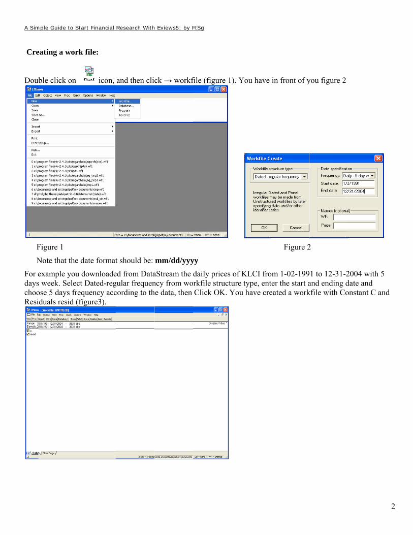
Cre

Doub

F

N

For edayschooResi

mple Guide to S

eating a wor

ble click on

Figure 1

Note that the

example yous week. Selecose 5 days frduals resid (

Start Financial

rk file:

icon,

e date format

u downloadect Dated-regrequency acc(figure3).

Research With

and then clic

t should be:

ed from Datagular frequencording to th

h Eviews5; by F

ck → workf

mm/dd/yyy

aStream the ncy from wohe data, then

FtSg

file (figure 1

yy

daily prices rkfile structuClick OK. Y

). You have

of KLCI froure type, entYou have cre

in front of y

Figure 2

om 1-02-199ter the start aeated a work

you figure 2

2

91 to 12-31-2and ending dkfile with Co

2004 with 5 date and onstant C and

2

d

A Simple Guide to Start Financial Research With Eviews5; by FtSg

3

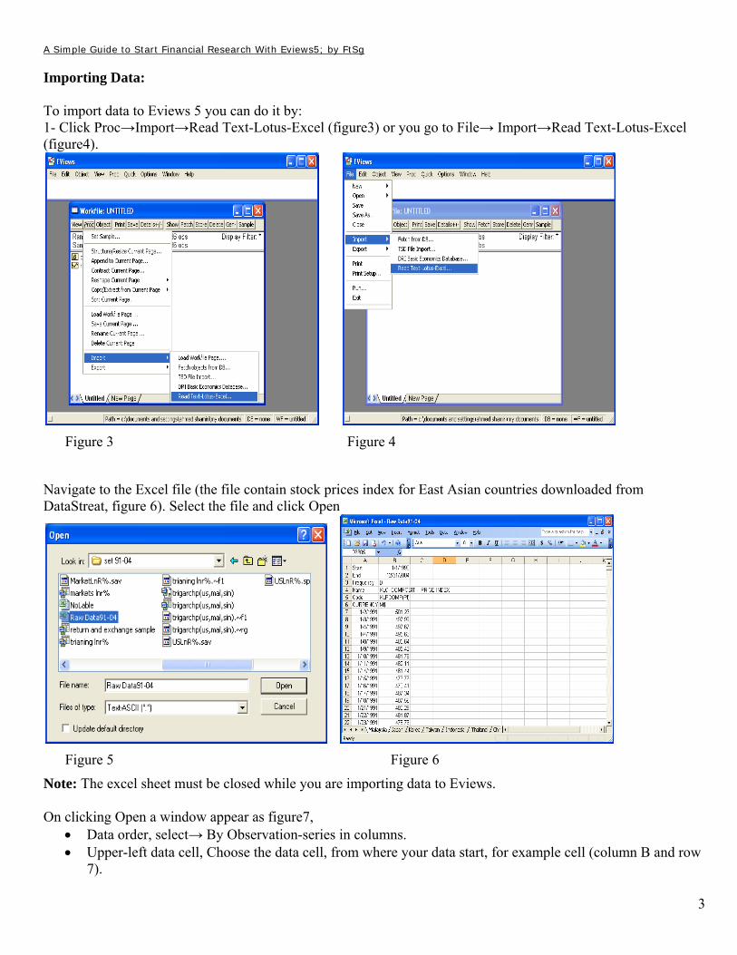
Importing Data: To import data to Eviews 5 you can do it by: 1- Click Proc→Import→Read Text-Lotus-Excel (figure3) or you go to File→ Import→Read Text-Lotus-Excel (figure4).

Figure 3 Figure 4

Navigate to the Excel file (the file contain stock prices index for East Asian countries downloaded from DataStreat, figure 6). Select the file and click Open

Figure 5 Figure 6

Note: The excel sheet must be closed while you are importing data to Eviews. On clicking Open a window appear as figure7,

• Data order, select→ By Observation-series in columns. • Upper-left data cell, Choose the data cell, from where your data start, for example cell (column B and row

7).


4

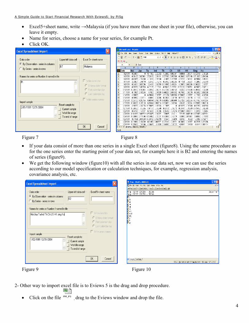
• Excel5+sheet name, write →Malaysia (if you have more than one sheet in your file), otherwise, you can leave it empty.

• Name for series, choose a name for your series, for example Pt. • Click OK.

Figure 7 Figure 8

• If your data consist of more than one series in a single Excel sheet (figure8). Using the same procedure as for the one series enter the starting point of your data set, for example here it is B2 and entering the names of series (figure9).

• We get the following window (figure10) with all the series in our data set, now we can use the series according to our model specification or calculation techniques, for example, regression analysis, covariance analysis, etc.

Figure 9 Figure 10

2- Other way to import excel file is to Eviews 5 is the drag and drop procedure.

• Click on the file , drag to the Eviews window and drop the file.


5

rt=100*log(pt/pt(-1)) rt=100*dlog(pt)

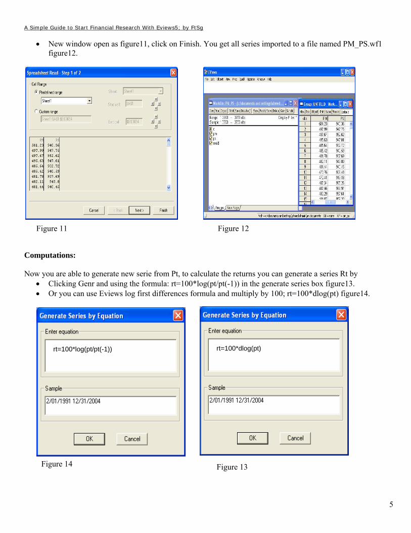
• New window open as figure11, click on Finish. You get all series imported to a file named PM_PS.wf1 figure12.

Figure 11 Figure 12

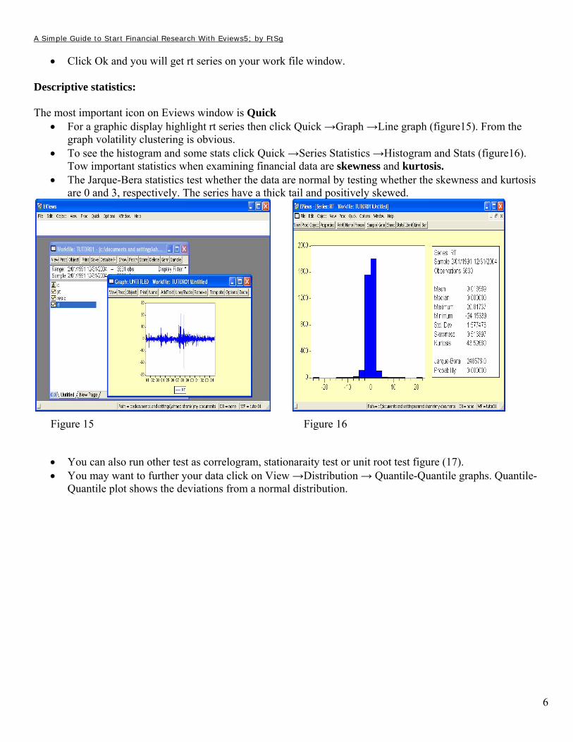
Computations: Now you are able to generate new serie from Pt, to calculate the returns you can generate a series Rt by

• Clicking Genr and using the formula: rt=100*log(pt/pt(-1)) in the generate series box figure13. • Or you can use Eviews log first differences formula and multiply by 100; rt=100*dlog(pt) figure14.

Figure 14 Figure 13


6

• Click Ok and you will get rt series on your work file window.

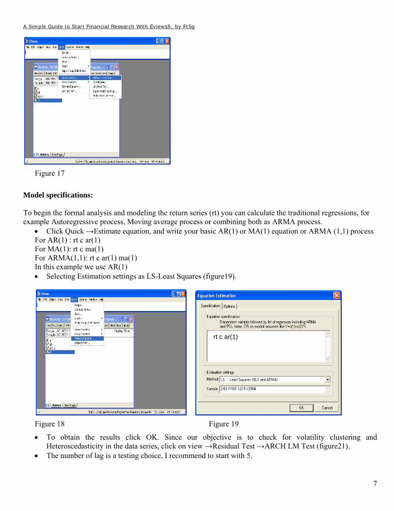
Descriptive statistics: The most important icon on Eviews window is Quick

• For a graphic display highlight rt series then click Quick →Graph →Line graph (figure15). From the graph volatility clustering is obvious.

• To see the histogram and some stats click Quick →Series Statistics →Histogram and Stats (figure16). Tow important statistics when examining financial data are skewness and kurtosis.

• The Jarque-Bera statistics test whether the data are normal by testing whether the skewness and kurtosis are 0 and 3, respectively. The series have a thick tail and positively skewed.

Figure 15 Figure 16

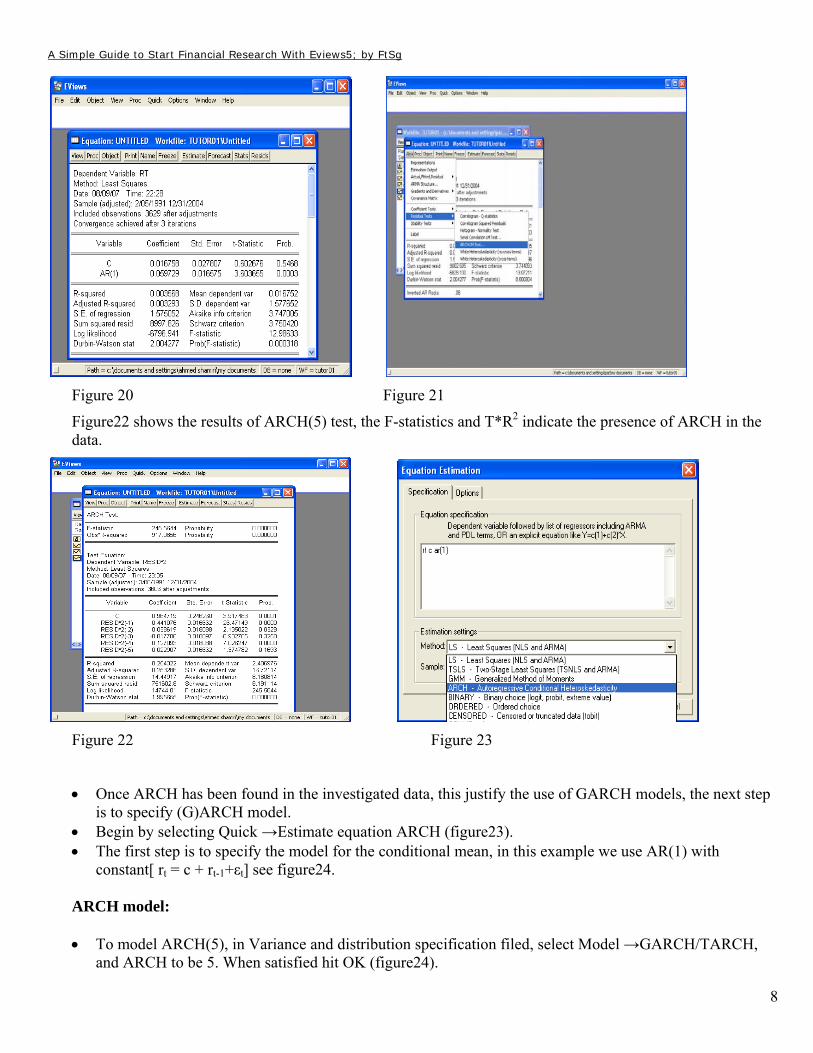
• You can also run other test as correlogram, stationaraity test or unit root test figure (17). • You may want to further your data click on View →Distribution → Quantile-Quantile graphs. Quantile-

Quantile plot shows the deviations from a normal distribution.


7

Figure 17

Model specifications: To begin the formal analysis and modeling the return series (rt) you can calculate the traditional regressions, for example Autoregressive process, Moving average process or combining both as ARMA process.

• Click Quick →Estimate equation, and write your basic AR(1) or MA(1) equation or ARMA (1,1) process For AR(1) : rt c ar(1) For MA(1): rt c ma(1) For ARMA(1,1): rt c ar(1) ma(1) In this example we use AR(1) • Selecting Estimation settings as LS-Least Squares (figure19).

Figure 18 Figure 19

• To obtain the results click OK. Since our objective is to check for volatility clustering and Heteroscedasticity in the data series, click on view →Residual Test →ARCH LM Test (figure21).

• The number of lag is a testing choice, I recommend to start with 5.

rt c ar(1)


8

Figure 20 Figure 21

Figure22 shows the results of ARCH(5) test, the F-statistics and T*R2 indicate the presence of ARCH in the data.

Figure 22 Figure 23

• Once ARCH has been found in the investigated data, this justify the use of GARCH models, the next step is to specify (G)ARCH model.

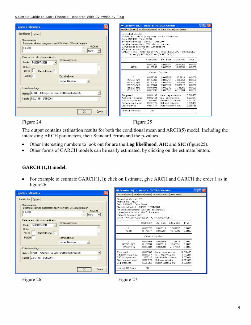
• Begin by selecting Quick →Estimate equation ARCH (figure23). • The first step is to specify the model for the conditional mean, in this example we use AR(1) with

constant[ rt = c + rt-1+εt] see figure24. ARCH model: • To model ARCH(5), in Variance and distribution specification filed, select Model →GARCH/TARCH,

and ARCH to be 5. When satisfied hit OK (figure24).


9

Figure 24 Figure 25

The output contains estimation results for both the conditional mean and ARCH(5) model. Including the interesting ARCH parameters, their Standard Errors and the p-values.

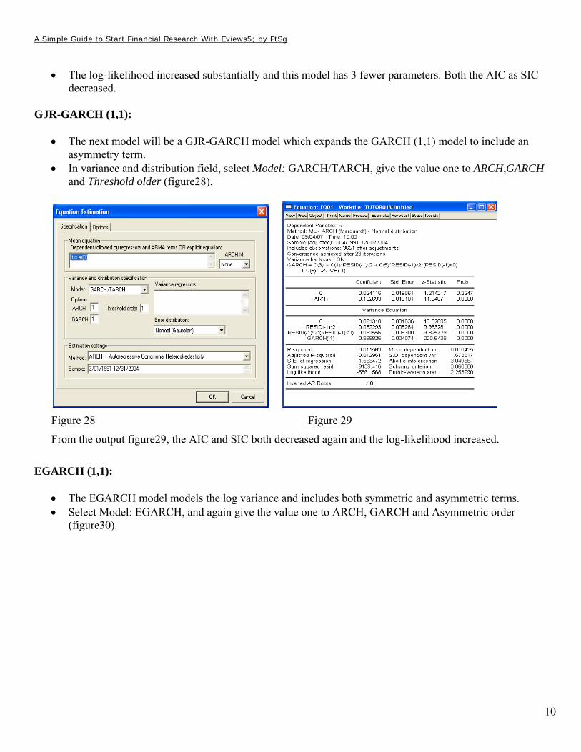
• Other interesting numbers to look out for are the Log likelihood, AIC and SIC (figure25). • Other forms of GARCH models can be easily estimated, by clicking on the estimate button. GARCH (1,1) model: • For example to estimate GARCH(1,1); click on Estimate, give ARCH and GARCH the order 1 as in

figure26

Figure 26 Figure 27


10

• The log-likelihood increased substantially and this model has 3 fewer parameters. Both the AIC as SIC

decreased. GJR-GARCH (1,1):

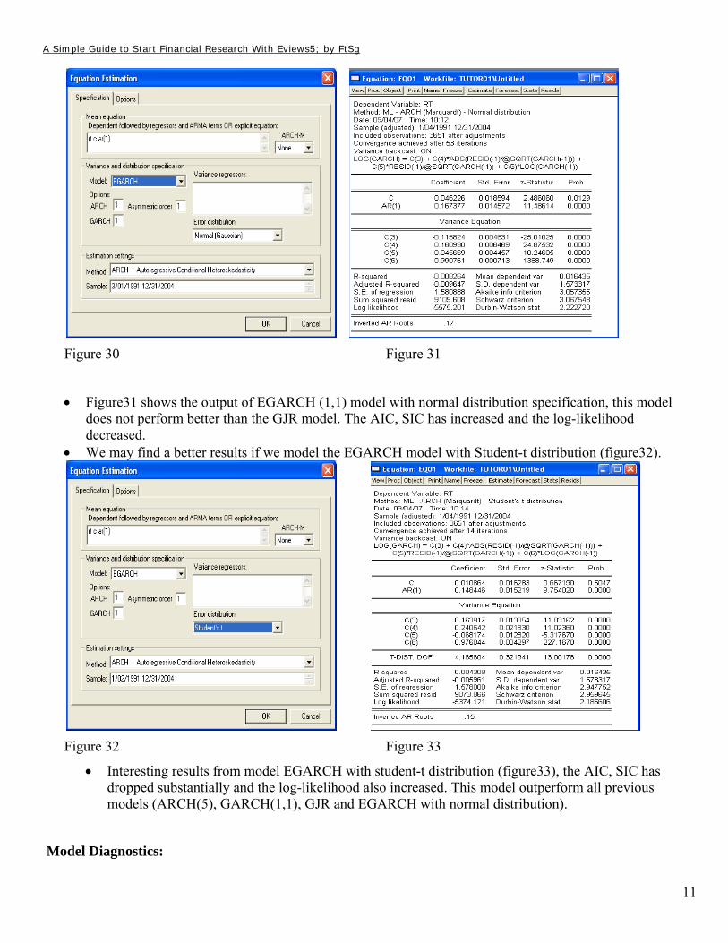
• The next model will be a GJR-GARCH model which expands the GARCH (1,1) model to include an asymmetry term.

• In variance and distribution field, select Model: GARCH/TARCH, give the value one to ARCH,GARCH and Threshold older (figure28).

Figure 28 Figure 29

From the output figure29, the AIC and SIC both decreased again and the log-likelihood increased.

EGARCH (1,1):

• The EGARCH model models the log variance and includes both symmetric and asymmetric terms. • Select Model: EGARCH, and again give the value one to ARCH, GARCH and Asymmetric order

(figure30).


11

Figure 30 Figure 31

• Figure31 shows the output of EGARCH (1,1) model with normal distribution specification, this model does not perform better than the GJR model. The AIC, SIC has increased and the log-likelihood decreased.

• We may find a better results if we model the EGARCH model with Student-t distribution (figure32).

Figure 32 Figure 33

• Interesting results from model EGARCH with student-t distribution (figure33), the AIC, SIC has dropped substantially and the log-likelihood also increased. This model outperform all previous models (ARCH(5), GARCH(1,1), GJR and EGARCH with normal distribution).

Model Diagnostics:


12

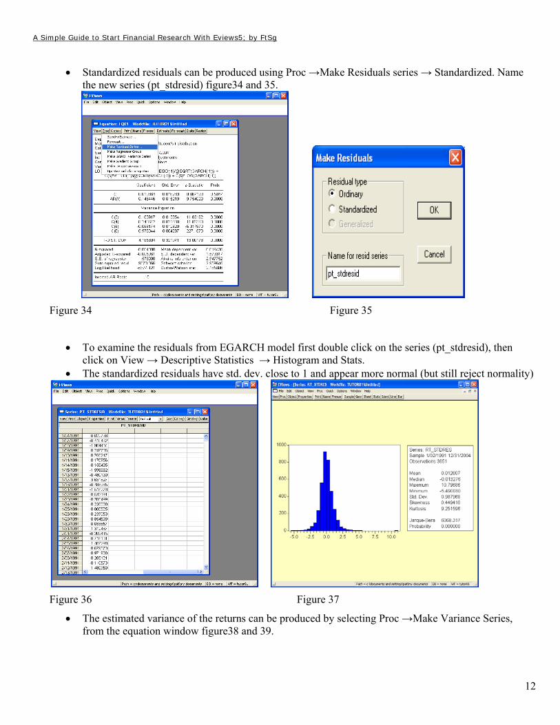
• Standardized residuals can be produced using Proc →Make Residuals series → Standardized. Name

the new series (pt_stdresid) figure34 and 35.

Figure 34 Figure 35

• To examine the residuals from EGARCH model first double click on the series (pt_stdresid), then click on View → Descriptive Statistics → Histogram and Stats.

• The standardized residuals have std. dev. close to 1 and appear more normal (but still reject normality)

Figure 36 Figure 37

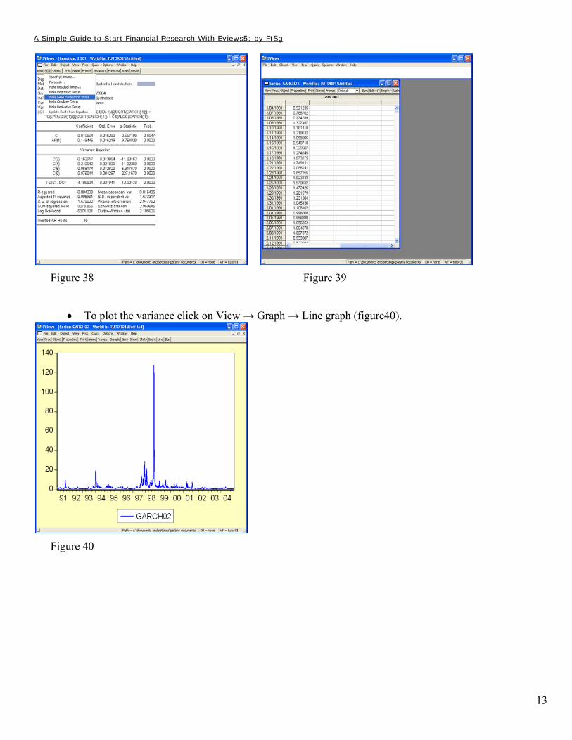
• The estimated variance of the returns can be produced by selecting Proc →Make Variance Series, from the equation window figure38 and 39.


13

Figure 38 Figure 39

• To plot the variance click on View → Graph → Line graph (figure40).

Figure 40


14

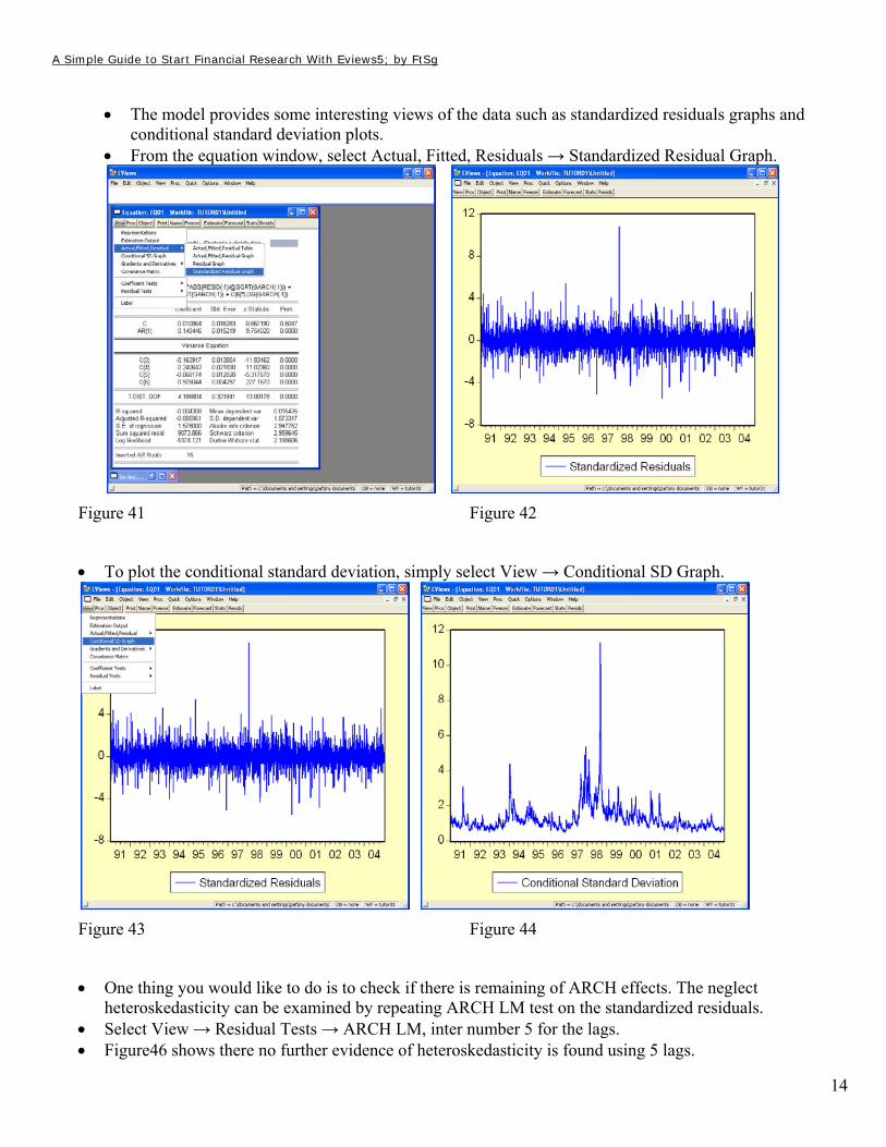
• The model provides some interesting views of the data such as standardized residuals graphs and

conditional standard deviation plots. • From the equation window, select Actual, Fitted, Residuals → Standardized Residual Graph.

Figure 41 Figure 42

• To plot the conditional standard deviation, simply select View → Conditional SD Graph.

Figure 43 Figure 44

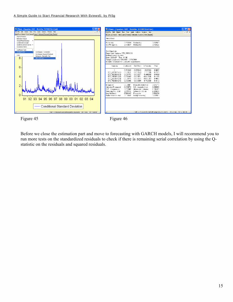
• One thing you would like to do is to check if there is remaining of ARCH effects. The neglect heteroskedasticity can be examined by repeating ARCH LM test on the standardized residuals.

• Select View → Residual Tests → ARCH LM, inter number 5 for the lags. • Figure46 shows there no further evidence of heteroskedasticity is found using 5 lags.


15

Figure 45 Figure 46

Before we close the estimation part and move to forecasting with GARCH models, I will recommend you to run more tests on the standardized residuals to check if there is remaining serial correlation by using the Q-statistic on the residuals and squared residuals.

a simple guide to start financial research with eviews 5 simple guide to start financial...

Documents