SANDIA REPORT SAND2012-1343 Unlimited Release Printed June 2012

A Simple Approach to Modeling Ductile Failure Gerald W. Wellman Prepared by Sandia National Laboratories Albuquerque, New Mexico 87185 and Livermore, California 94550

Sandia National Laboratories is a multi-program laboratory managed and operated by Sandia Corporation, a wholly owned subsidiary of Lockheed Martin Corporation, for the U.S. Department of Energy's National Nuclear Security Administration under contract DE-AC04-94AL85000.

Approved for public release; further dissemination unlimited.

2

Issued by Sandia National Laboratories, operated for the United States Department of Energy by Sandia Corporation. NOTICE: This report was prepared as an account of work sponsored by an agency of the United States Government. Neither the United States Government, nor any agency thereof, nor any of their employees, nor any of their contractors, subcontractors, or their employees, make any warranty, express or implied, or assume any legal liability or responsibility for the accuracy, completeness, or usefulness of any information, apparatus, product, or process disclosed, or represent that its use would not infringe privately owned rights. Reference herein to any specific commercial product, process, or service by trade name, trademark, manufacturer, or otherwise, does not necessarily constitute or imply its endorsement, recommendation, or favoring by the United States Government, any agency thereof, or any of their contractors or subcontractors. The views and opinions expressed herein do not necessarily state or reflect those of the United States Government, any agency thereof, or any of their contractors. Printed in the United States of America. This report has been reproduced directly from the best available copy. Available to DOE and DOE contractors from U.S. Department of Energy Office of Scientific and Technical Information P.O. Box 62 Oak Ridge, TN 37831 Telephone: (865) 576-8401 Facsimile: (865) 576-5728 E-Mail: reports@adonis.osti.gov Online ordering: http://www.osti.gov/bridge Available to the public from U.S. Department of Commerce National Technical Information Service 5285 Port Royal Rd. Springfield, VA 22161 Telephone: (800) 553-6847 Facsimile: (703) 605-6900 E-Mail: orders@ntis.fedworld.gov Online order: http://www.ntis.gov/help/ordermethods.asp?loc=7-4-0#online

3

SAND2012-1343 Unlimited Release Printed June 2012

A Simple Approach to Modeling Ductile Failure

Gerald W. Wellman Structural Mechanical Engineering Department

Sandia National Laboratories P.O. Box 5800

Albuquerque, New Mexico 87185

Abstract

Sandia National Laboratories has the need to predict the behavior of structures after the occurrence of an initial failure. In some cases determining the extent of failure, beyond initiation, is required, while in a few cases the initial failure is a design feature used to tailor the subsequent load paths. In either case, the ability to numerically simulate the initiation and propagation of failures is a highly desired capability. This document describes one approach to the simulation of failure initiation and propagation.

4

ACKNOWLEDGEMENTS The author wishes to express his appreciation to the following: Joe Jung, John Pott, and Jim Redmond, a series of managers, who provided support and stable funding for this project over several years. Brendan Rogillio, Phillip Reu, and Bonnie Antoun who produced the excellent experiments referenced throughout this document. Mike Stone who was instrumental in the implementation of this techniques in SNL legacy codes. Bill Scherzinger, Vicki Porter, and Tim Shelton who accomplished most of the implementation while educating the author in the SIERRA mechanics suite of codes. Bill Scherzinger, Arne Gullerud, and Martin Heinstein who provided many helpful discussions while ensuring that sins against mechanics were kept to a minimum. Kristin Dion, Nicole Breivik, Frank Dempsey, Spencer Grange, and Jeff Gruda early users who provided numerous suggestions for improvement.

5

CONTENTS

INTRODUCTION…………………………………………………………………………………………………..11

TEARING PARAMETER………………………………………………………………………………………….12

ENERGY DISSIPATION…………………………………………………………………………………………...16

FAILUREALGORITHM…………………………………………………………………………………………...18

PARAMETER ESTIMATION……………………………………………………………………………………..20

IMPLEMENTATION………………………………………………………………………………………………23

THREE-HOLE TENSION EXPERIMENT……………………………………………………………………….25

EXAMPLES...……………………………………………………………………………………………………….40

WARTS………………………………………………………………………………………………………………46

CONCLUSIONS…………………………………………………………………………………………………….50

REFERENCES………………………………………………………………………………………………………50

FIGURES Figure 1. 6061-T6 room temperature smooth bar tensile data with Cauchy-stress, Logarithmic-strain and the result of a finite element analysis of the tensile test using the extracted Cauchy-stress, Logarithmic-strain………………………………………………………………………...14 Figure 2. Comparison of experiment and analysis for 6061-T6 notched tensile MAVEN project data showing the improvement in failure prediction using the modified tearing parameter……15 Figure 3. Comparison of experiment and analysis for 6061-T6 notched tensile WES project data showing the improvement in failure prediction using the modified tearing parameter…………15 Figure 4. Graphical explanation of energy dissipation during element failure…………………17 Figure 5. Multilevel Solution Algorithm for Quasistatic Failure……………………………….19 Figure 6. Algorithm for Extracting Cauchy-Stress, Plastic Logarithmic-Strain from Standard Tensile Test Engineering-Stress, Engineering-Strain Data……………………………………...20 Figure 7. Extraction of Cauchy-Stress, Plastic Logarithmic Strain for 304 L Stainless Steel at Room Temperature Showing the Accuracy of the Process (Black Versus Green Curves)……..21 Figure 8. Drawing of the Three-Hole Tension Specimen……………………………………….26 Figure 9. Solid model of the Three-Hole Tension Specimen…………………………………...26 Figure 10. Tensile test data for 304L stainless steel…………………………………………….28 Figure 11. Tensile test data for 17-4PH stainless steel………………………………………….28

6

Figure 12. Tensile test data for 6061-T6 Aluminum……………………………………………29 Figure 13. Cauchy-Stress versus Logarithmic-Strain for the 304L Stainless Steel…………….30 Figure 14. Cauchy-Stress versus Logarithmic-Strain for the 17-4PH Stainless Steel………….31 Figure 15. Cauchy-Stress versus Logarithmic-Strain for the 6061-T6 Aluminun………………31 Figure 16. Load versus Load-Line Displacement for Three-Hole Tension Specimen of 304L Stainless Steel……………………………………………………………………………………32 Figure 17. Inferred Crack Extension versus Load-Line Displacement for Three-Hole Tension Specimen of 304L Stainless Steel………………………………………………………………..32 Figure 18. Load versus Load-Line Displacement for Three-Hole Tension Specimen of 17-4 PH Stainless Steel……………………………………………………………………………………33 Figure 19. Inferred Crack Extension versus Load-Line Displacement for Three-Hole Tension Specimen of 17-4 PH Stainless Steel……………………………………………………………33 Figure 20. Load versus Load-Line Displacement for Three-Hole Tension Specimen of 6061-T6 Aluminum………………………………………………………………………………………34 Figure 21. Inferred Crack Extension versus Load-Line Displacement for Three-Hole Tension Specimen of 6061-T6 Aluminum……………………………………………………………….34 Figure 22. Coarsest mesh (0.02x0.02x0.01 inch) used in the analysis of the three-hole tension specimen…………………………………………………………………………………………35 Figure 23. Finest mesh (0.0025x0.0025x0.0025 inch) used in the analysis of the three-hole tension specimen…………………………………………………………………………………36 Figure 24. Comparison between experimental and simulation results of load versus displacement for 304L stainless steel 3-hole tension…………………………………………………………...37 Figure 25. Comparison between experimental and simulation results of load versus displacement for 17-4PH stainless steel 3-hole tension………………………………………………………...38 Figure 26. Comparison between experimental and simulation results of load versus displacement for 6061-T6 aluminum 3-hole tension…………………………………………………………...38 Figure 27. Comparison between experimental and simulation results of crack extension versus displacement for 304 stainless steel 3-hole tension……………………………………………...39 Figure 28. Comparison between experimental and simulation results of crack extension versus displacement for 17-4PH stainless steel 3-hole tension………………………………………….39

7

Figure 29. Comparison between experimental and simulation results of crack extension versus displacement for 6061-T6 aluminum 3-hole tension…………………………………………….40 Figure 30. Drawing of the challenge 1-A compact specimen with kinked-slot key-hole………42 Figure 31. Comparison of experiment to simulation for load versus displacement for the ductile failure X-prize challenge 1-A……………………………………………………………………43 Figure 32. Comparison of experiment to simulation for load versus displacement for the ductile failure X-prize challenge 1-B…………………………………………………………………….44 Figure 33. Comparison of experiment to simulation for deformed shape and crack path for the ductile failure X-prize challenge 1-B; left hand side is the experiment, right hand side is the pre-test analysis………………………………………………………………………………………45 Figure 34. Typical results from the quasistatic analysis of the “pipe-bomb” specimen just prior instability and failure; a) Temperature in degrees Kelvin, b) plastic strain, c) depiction of pre-failure bulge……………………………………………………………………………………...46 Figure 35. Comparison of experiment to simulation for deformed shape of the pipe-bomb after burst. Experiment on the left hand side, Analysis on the right hand side………………………..47 Figure 36. Potential effect of load increment on accuracy of energy dissipation……………….48 TABLES Table 1. Comparison of CCOS from simulation fit to experiment and from parameter estimation scheme ……………………………………………………………………………...41

8

9

Introduction Historically, engineers have been asked to ensure that structures of their components do not fail. There are usually three parts to this approach. First, the stress and strains in a component are computed. In the past, this has typically been done using linear-elastic theory. In present practice, the use of non-linear constitutive models (plasticity, creep, etc.) has become routine. Second, a factor-of-safety is obtained by comparing the stress or strain computed in the first step to a criterion that is appropriate to the structure under consideration and the type of analysis performed. Finally, in the third step, the engineer makes a determination that the component of structure is acceptable. This determination is based on empirical evidence with similar structures or engineering judgment. This approach has been and continues to be very successful in the design of structures, particularly where there is ample historical evidence. The design codes for buildings, pressure vessels and piping, maritime vessels, etc. are among the more visible successful applications of this approach. Increasingly, engineers (structural analysts) at Sandia National Laboratories are being asked to perform failure analyses, to determine fitness for service, and assess consequences of failure. In many cases, the determination of the initiation of a failure is all that is required. This looks very similar to the traditional approach. However, there is a class of problems where the ability to simulate the entire failure process from initiation to arrest or separation is required. Some such applications are the determination of how the failure progression of a noncritical component affects the load transfer to a critical component, determination if the extent of cracking will render a component inoperable or affect hermeticity, and the class of components where failure of a structural member at the proper time and at the proper location is part of the design function. Answers to these questions require tools beyond those used for the more traditional factor-of-safety computations. One of these new tools, a technique to simulate ductile failure of metals (both failure initiation and propagation) is the subject of this report. There are three general approaches to the modeling of failure: fracture mechanics, damage mechanics, and cohesive zones. The field of fracture mechanics can be argued to have its initiation with Griffith’s work in 1920 [1]. However, the widespread development and use of modern fracture mechanics is generally accepted to have begun in the mid 1940’s. Now, nearly seventy years later, while there are still areas of active research, the field of fracture mechanics must be considered to be mature. No effort will be made to provide an exhaustive review of the literature, instead, a select few excellent texts the author has found particularly helpful will be cited[2][3][4]. Some of the fracture mechanics techniques used to predict ductile tearing are; LEFM – with plastic zone correction, Failure assessment Diagram, Dugdale strip-yield, KR – Resistance Curve, JR – Resistance Curve, Crack Tip Opening Displacement, Crack Tip Opening Angle, and Tearing Modulus Methods. An excellent discussion of these methods along with comparison to data is provided by Newman and Loss[5]. Fracture mechanics techniques suffer from their need to incorporate a single dominant preexisting crack. This crack simply does not exist for many problems of interest. In addition, fracture mechanics, while quite successful for predicting crack initiation, have not demonstrated similar success for simulating crack propagation. The field of damage mechanics, generally accepted to have started with Kachanov’s 1958 work[6], is slightly newer than fracture mechanics. An excellent review of this field is provided

10

by Krajcinovic[7,8,9]. Crack propagation is modeled in damage mechanics through the introduction of an internal variable and a rate equation which quantify the evolution of damage and thus affect the constitutive response. Macroscopic failure (cracking) occurs when this state variable reaches a critical value or its rate of change becomes sufficiently large. Damage mechanics has proven to be much more successful at simulation of increasing porosity and distributed cracking than the formation and propagation of a single dominant crack. The development of cohesive zone technology can be argued to have started with Barrenblatt [10] and Dugdale [11]. Fundamentally, a cohesive zone model is used to characterize the fracture process through the introduction of a traction-separation rule on the crack plane. In theory, the traction-separation rule captures the work of separation per unit area of new free surface creation. The author found the work of Tvergaard and Hutchinson [12,13], de Borst,Remmers, and Needleman [14,15], and Bazant and Oh [16] most helpful to the work presented here. A major drawback to the cohesive zone technique is the requirement to predetermine the crack propagation path in order to place the cohesive zones in the correct locations. Secondarily, for plasticity, the value used for the maximum traction in the cohesive zone is ambiguous. The value of the hydrostatic stress state at failure can significantly change the maximum traction. Ubiquitous placement of cohesive zones, between every element, in an attempt to minimize the need to predetermine the crack path leads to unphysical added compliance in the simulation. This is highly undesirable. To minimize the additional compliance, the cohesive zones can be either activated by a trigger from the constitutive model or automatically inserted. While numerically very different, these two techniques generate nearly identical behavior. A source of uncertainty with either of these two techniques is the decision as to which side of an element to either activate the preexisting cohesive zone or to insert one. This decision can affect the subsequent response within the constitutive model particularly for elements local to the newly activated or inserted cohesive zones. In addition, the cohesive zone approach appears to work best when the cohesive zone is active over several (3 to 10) elements. This could imply that the crack path must still be correctly predicted. The technique presented here has the weakest ties to classical fracture mechanics. It draws heavily from both damage mechanics and cohesive zone approaches. Similar to damage mechanics, a local criterion is computed to determine the initiation of failure. The subsequent stress decay post initiation is similar to a cohesive zone approach. Within a failing element, the stress is decayed to zero over a specified amount of strain. This technique has been referred to as a “distributed cohesive zone” or “crack-band.” TEARING PARAMETER The start of the effort documented here was the search for an improved method of predicting failure (or alternately assessing margin against failure) of exclusion region barriers. The purpose of an exclusion region barrier is prevention of any energy source (electrical, optical, mechanical, etc.) from reaching the critical components that initiate the firing sequence of a nuclear weapon while that weapon is still capable of operation. Improved methodology for predicting the onset of failure allowed increased rigor in assessing safety margins, as well as improved design decisions to increase safety margins. In the search for an improved method for predicting the onset of a failure, six different failure criteria were assessed [17]. The parameter proposed by Brozzo, et. al.

11

[18] was selected from this study. This parameter takes the form of an evolution integral of the stress state integrated over the plastic strain as follows:

pmT

T dTP

3

2

Where TP is the tearing parameter, T is the maximum principal stress, m is the hydrostatic

component of the stress tensor (trace of the stress), and p is the plastic strain. For uniform,

uniaxial tensile stress, the stress state term is one. However, most ductile metal alloys experience a tensile instability (necking) during tensile testing. After necking begins, the stress state is no longer uniaxial or uniform and the stress state takes on a value different from unity. Thus, the critical value of the tearing parameter is almost never the strain-to-failure which it would be if the stress state term were unity. Further investigation of the tearing parameter revealed the need for modification of Brozzo’s original formulation. The first modification was the inclusion of a Heaviside bracket on the maximum principal stress. That is, if the maximum principal stress is compressive (negative) the increment to the tearing parameter is zero. Thus, there is no increase in “damage” for compressive stress states, nor is there “damage healing” for compressive states. The second modification resulted from the investigation of notched tensile test results. Two sets of round bar and notched tensile tests were performed [19,20] on different heats of 6061-T6 aluminum. These data sets will be referred to by the names of the projects they supported, MAVEN and WES. The Cauchy-stress versus logarithmic-strain behavior suitable for use in a large deformation plasticity finite element analysis code was extracted from the engineering-stress versus engineering-strain tensile data according to the procedure discussed later in this report. These fitting results are shown in Figure 1. The solid curves labeled “data” are the experimental engineering stress-strain curves (smoothed to eliminate the 60-cycle vibration seen in the original data). The solid curves labeled “true” are the Cauchy-stress versus logarithmic-strain curves. The curves labeled “fit” are the results of a simulation of the tensile test using the “true” curve as input to the finite element code. The tearing parameter was determined by evaluating the integral shown above (referred to as TP-old). For the MAVEN data, TP-old at failure in the smooth-bar tensile test was 0.83. For the WES data, TP-old was 0.81. Comparison between the simulations and the experimental results for the notched tensile tests showed excessive ductility for the simulations. Because the simulation of the smooth bar tensile test agreed with the test results (calibrated to so), it was suspected that the stress state was not contributing sufficiently to the value of TP-old. Several modifications were tried with raising the stress-state portion of the integral to the fourth power being the most successful. This will be referred to a TP-new in this section. TP-new is shown in the following equation.

pmT

T dTP

4

3

2

Using this modified Brozzo equation, TP-new for the MAVEN data was 1.57 and for the WES data TP-new was 1.52.

12

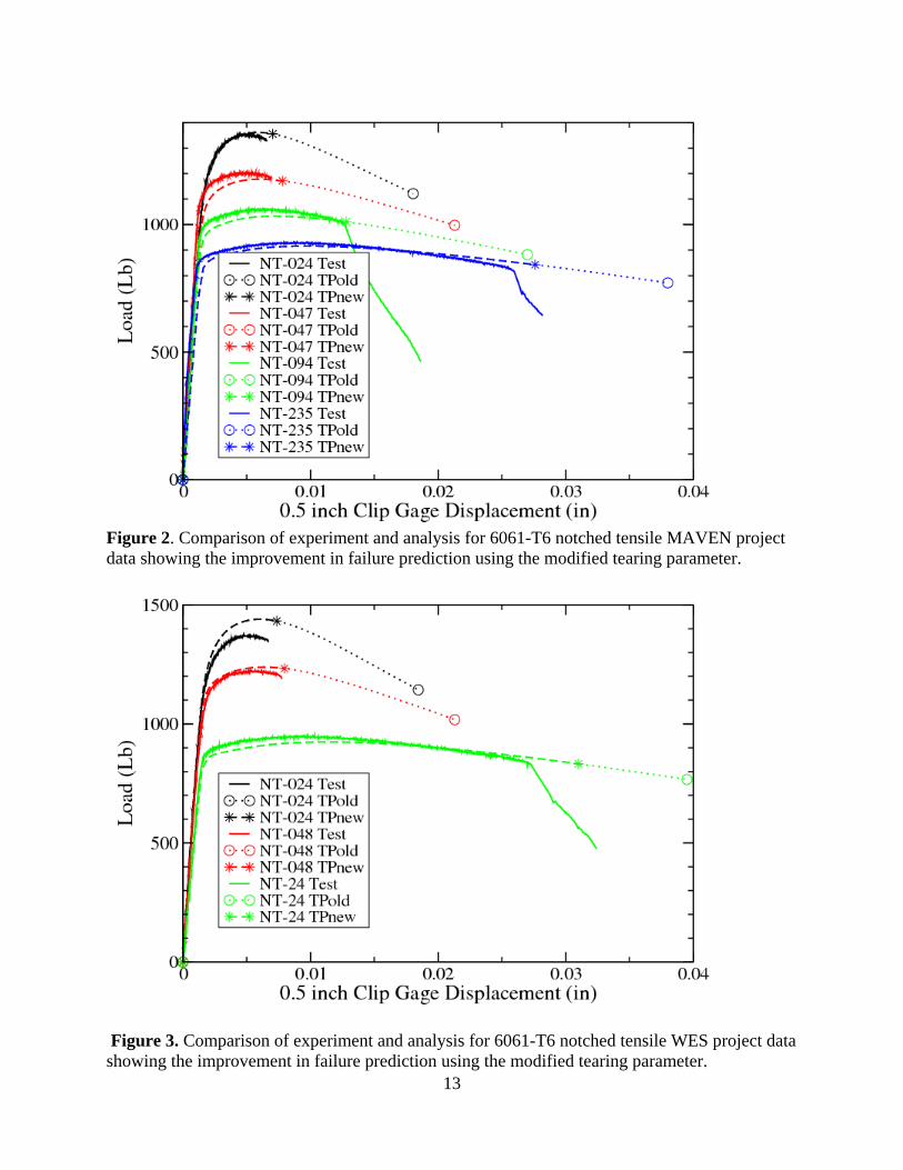
Figure 1. 6061-T6 room temperature smooth bar tensile data with Cauchy-stress, Logarithmic-strain and the result of a finite element analysis of the tensile test using the extracted Cauchy-stress, Logarithmic-strain The notched tensile tests were then simulated using the Cauchy-stress versus logarithmic-strain constitutive behavior extracted from the smooth-bar tensile test results. Failure was assumed when the tearing parameter (either TP-old or TP-new) reached the value computed for the smooth bar tensile test. The simulations of the notched tensile tests are compared to the experimental results in Figures 2 and 3. As shown in Figures 2 and 3, simulations of failure using TP-new match the notched tensile data much more accurately than do those using TP-old. Therefore, throughout the rest of this report, the tearing parameter using the stress-state raised to the power of 4 (TP-new) will be used and referred to simply as the tearing parameter or TP.

13

Figure 2. Comparison of experiment and analysis for 6061-T6 notched tensile MAVEN project data showing the improvement in failure prediction using the modified tearing parameter.

Figure 3. Comparison of experiment and analysis for 6061-T6 notched tensile WES project data showing the improvement in failure prediction using the modified tearing parameter.

14

ENERGY DISSIPATION The use of an energy dissipation technique for eliminating the element size effect in crack propagation used in this work was motivated by Bazant’s [21] work on quasi-brittle failure in concrete. The literature describing energy dissipation during crack propagation has proliferated in the subsequent years. The reader is directed to the excellent review article by de Borst [22] for a more thorough examination of these techniques. The only length scale available using the technique described in this report for modeling ductile failure is the element size. Thus, in the most literal interpretation, the finite element mesh becomes a material property. In actuality, this can be mitigated by making the energy dissipation term a function of the element size. An algorithm to automatically adjust the energy dissipation to suit the current element size is under development and should be available soon. However, at the present time, the energy dissipation is still a user defined parameter and care must be exercised to input a value that is appropriate to the size of elements through which the crack is expected to grow. The energy dissipation term is named the critical crack opening strain. At initiation of failure (the tearing parameter described above reaches its critical value), the direction of the maximum principal stress is calculated and saved. The crack opening direction is assumed to be aligned with the maximum principal stress direction at failure initiation. That is, once failure is initiated within an element, the crack opening direction can no longer change due to load redistribution or even changes in the applied loading. For a failing element, the component of the strain increment (not the total strain) in the crack opening direction is used to isotropically and linearly decay the element stresses. More accurately, this technique should be called energy density dissipation. However, when integrated over the element volume, energy is dissipated. This technique has been referred to as a distributed or diffuse cohesive zone. It is a three-dimensional analog to the more familiar two-dimensional cohesive zone with the advantage that there is no need to predefine the crack direction. The user input, critical crack opening strain parameter, defines the stress decay rate by forcing the element stresses to be zero when the crack opening strain reaches its critical value. This scheme is shown graphically, for one dimension, in Figure 4. A scheme to estimate the value of the critical crack opening strain appropriate to a specific material and element size is given in the section on parameter estimation.

15

Figure 4. Graphical explanation of energy dissipation during element failure The actual mechanism of the stress decay was accomplished using a constitutive model. Initially, a hypo-elastic model was used. A secant modulus was estimated from the stress and strain state at failure initiation. This modulus was then decreased to achieve the desired linear reduction in the stress state with increasing crack opening strain. This stress decay technique created a certain amount of ambiguity over how to treat transient unloading waves not uncommon in transient dynamic analyses. Despite this ambiguity, the behavior of this technique was acceptable for transient dynamics. However, it did not exhibit the desired robustness in quasistatic analyses. Changing the stress decay mechanism from elasticity to plasticity greatly improved the speed and robustness in the implementation used here. In the plasticity based stress decay algorithm, the stress state at failure initiation is used to define the radius of a failure (yield) surface. (This failure (yield) surface is independent of the actual yield surface for the plasticity computations prior to failure.) The radius of the failure (yield) surface is decreased as a function of the crack opening strain and then the stress state is decayed (radial return algorithm) to lie on that new failure (yield) surface. For cases of complete constraint, this technique will reduce the stress state to a zero deviatoric component but can allow a remaining hydrostat. Therefore, the hydrostat is also checked and is decayed appropriately according to the crack opening strain. This technique allows unloading and reloading behavior to be handled unambiguously. In addition, in the

Failure Initiation

Crack Opening Strain

16

implementation in the Sierra based mechanics quasistatics codes used here, the equilibrium iterations are both faster and more robust. FAILURE ALGORITHM The tearing parameter was first conceived as a criterion to estimate the initiation of tearing in a ductile material in the absence of a single dominant crack. The tearing parameter proved to be successful at predicting ductile failure initiation so an attempt was made to model ductile crack propagation as a series of initiation events in a transient dynamics code. The implementation of crack propagation was carried out entirely within the constitutive model. This was done by providing four independent paths through the constitutive model controlled by a flag that indicated the cracking status. The first path through the constitutive model was simply a classical plasticity model. Several plasticity models were implemented with the favored one having a von Mises yield surface, strain-hardening defined by a series of line segments in Cauchy-stress, Logarithmic-strain, and radial return. The second path through the constitutive model was for elements that start failing in the current step. In this path, the direction of the maximum principal stress is computed and the strain increment is partitioned into plasticity and crack opening strain portions. The plasticity portion is used to compute the stress and strain state at failure. The crack opening strain portion is used to decay the stress from the state computed using the plasticity portion. In general terms, path 2 turns the corner from plasticity to failure. The third path does nothing but stress decay based on the crack opening strain. Finally, the fourth path just returns a zero stress state regardless of the strain increment. This path can be considered redundant because any element that could take this path should have already be deleted.This technique was successful in the sense that useful simulations were obtained despite the noted mesh sensitivities. Initial attempts to transition this technique to a quasistatic application using an iterative solver proved to be unsuccessful because of spurious cracking predicted during the procedure to iterate to an equilibrium solution. The two primary issues with quasistatics were the arbitrarily large load step size and the seemingly arbitrary iterative path to a converged equilibrium solution. The resolution of both these issues was achieved by only allowing an element to begin cracking from a converged solution. This was first implemented in quasistatics code that used a dynamic relaxation solution scheme [23]. Independently, Heinstein [24] introduced the concept of a “multilevel solver” in the Sierra based mechanics codes to improve convergence of poorly conditioned problems. This is done by holding fixed some variables that would ordinarily be free to change in the fully nonlinear iteration. This technique has applications such as contact and nearly incompressible materials. Allowing an element to begin failing only from a converged state was a natural application for this technique. The multilevel solver algorithm for quasistatics failure is detailed in Figure 5. With the use of this algorithm, failure in a could be successfully modeled.

17

Figure 5. Multilevel Solution Algorithm for Quasistatic Failure PARAMETER ESTIMATION Elastic constants (Youngs’s modulus and Poisson’s ratio) are generally available from the literature. Use of such tabulated constants is completely adequate. Estimation of Young’s modulus from standard tensile testing, while possible, is subject to inaccuracies and discouraged. In constitutive models typically used for simulating failure (specifically those employed here), the use of the term yield stress or yield strength is a misnomer. Here we should more accurately use the term proportional limit rather than yield stress. The use of a 0.2% offset yield stress in a constitutive model that is attempting to capture the entire range of strain hardening gives rise to an inconsistency (kink) in the hardening curve. The assumption is made that the material is linear and elastic up to yield. At a 0.2% offset, clearly some plasticity has occurred. Thus to achieve a smooth curve, either the modulus or the start of the strain hardening curve must be adjusted. To alleviate this discrepancy, the use of the proportional limit is suggested. This makes the description of the material behavior within the constitutive model more realistic. The accuracy of the proportional limit is not critical for applications where the simulation will be extended to failure. Thus the ambiquity inherent in selecting a proportional limit (the reason for the 0.2% offset definition for yield strength) is not a significant problem. Failure of ductile metals occurs after appreciable plastic strain. For all the materials considered here, except 2024-T3 aluminum, failure occurs after the tensile instability (necking) in a tension test. Note: while compression or torsion testing is often used to explore the large strain regime, such tests are difficult to use to determine parameters used to define material failure criterion. Accurate simulation of stresses and strains post necking requires the use of large strain, large deformation (nonlinear geometry) formulations. In the finite element codes used in this study, the Cauchy-stress and plastic logarithmic-strain conjugates are employed. In order to derive the appropriate input parameters for such a finite element code, the Cauchy-stress and plastic logarithmic-strain must be obtained from materials property tests on the material of interest. While it is possible to perform a materials property test in which the true-stress and true-strain

1) Start new load step 2) Converge solution at lowest level (level 0-no new failure) 3) Any elements exceed failure criterion? No – go to 5 Yes – go to 4 4) Select element most exceeding criterion, mark that element for

“fail this step (path 2)” – go to 2 5) Change all elements “failing this step” to “failing (path 3)” 6) Mark all elements that have decayed to zero stress for element

deletion (path 4) 7) Update all state variables and go to 1

18

(analogous to Cauchy-stress and logarithmic-strain) are measured or at least deduced, such tests are extremely difficult and thus, such materials property data are rare. Standard test methods, that produce engineering stress versus engineering strain, exist for tensile testing which are quite simple and such data is readily available. It is possible to estimate the true-stress, true-stain from engineering stress-strain data assuming a uniform, uniaxial stress state and constant volume for plasticity. However, these assumptions are not valid for post necking behavior. To determine the entire Cauchy-stress, plastic logarithmic-strain response from a standard tensile test, it is necessary to solve an inverse problem. All the Cauchy-stress plastic logarithmic-strain data presented here was obtained through this inverse (perhaps optimization process is more appropriate) process.

Figure 6. Algorithm for Extracting Cauchy-Stress, Plastic Logarithmic-Strain from Standard Tensile Test Engineering-Stress, Engineering-Strain Data Solving the inverse problem is quite straight forward, albeit tedious. In general, a guess at the Cauchy-stress, plastic logarithmic-strain is used in a finite element simulation of a tensile test. The result of the simulation is then compared to the test data. This process is repeated until the result from the simulation is sufficiently close to the experimental data. This process uses the finite element analysis to separate structural behavior (necking, etc.) from the materials properties measured in a standard tensile test. The details of the algorithm employed to perform this process are shown in Figure 6. The algorithm above proved to be the more robust and faster than other optimization routines attempting to provide the same result. Use of an incremental fit reduced simulation time spent in the finite element program over routines that attempted to fit the entire hardening curve. This algorithm was scripted for use on LINUX workstations using

1. Read data, set-up template, initialize 2. New displacement increment – read restart if there is one 3. Initial hardening modulus from last converged increment 4. Simulate a displacement increment – proportional to strain increment. 5. Convert load to engineering stress and compare to experimental data 6. If simulated stress less than experimental data,

a. increase hardening modulus, b. go to 4

7. If simulated stress greater than experiment, a. decrease hardening modulus, b. go to 4

8. If simulation and experiment within tolerance, a. Extract logarithmic strain at end of increment from simulation. Subtract

elastic strains to get plastic logarithmic strain b. Compute Cauchy-stress at end of increment (use hardening modulus and

logarithmic strain increment) c. Enter plastic logarithmic-strain and Cauchy-stress in input template

9. If simulation engineering strain less than experimental maximum strain, a. Write restart b. Go to 2

10. If simulation engineering strain equal experimental maximum strain, End

19

PERL by Tim Shelton[25]. The script is available for use by anyone with access to the engineering sciences LAN. An example of the results of this inverse process for extracting Cauchy-stress, plastic logarithmic-strain from standard tensile test data is shown in Figure 7.

Figure 7. Extraction of Cauchy-Stress, Plastic Logarithmic Strain for 304 L Stainless Steel at Room Temperature Showing the Accuracy of the Process (Black Versus Green Curves). For those unfamiliar with large strain, large displacement computational frameworks, the magnitude of the stresses and strains in the Cauchy-stress, plastic Logarithmic-strain curve will seem very large. A simplified way to look at the differences between Engineering stress and strain and Cauchy-stress and Logarithmic-strain is that the engineering quantities are based on original, undeformed geometry while the Cauchy-stress and Logarithmic-strain reference current continuously deforming geometry. These large Logarithmic-strains occur over a very limited volume of the tensile specimen; basically within the necked region of the specimen. Therefore, unlike engineering strain which is assumed to be uniform over the reference gage length, Logarithmic strain will vary widely over the specimen from very high values in the necked region to values not too different from the engineering strain in less deformed regions. Likewise, the Cauchy-stress will be very high in the highly deformed necked region while it will be similar to the engineering stress near the mildly deformed grip region. Estimation of the failure initiation criterion (the tearing parameter) is quite simple. A simulation of the tensile specimen is performed up to the strain or displacement at which failure is seen in the tensile test. The maximum value of tearing parameter in the simulation at the last step of the

20

simulation is taken to be the critical value. This is probably a slightly high estimate of the tearing parameter because there will be some energy dissipation in propagating the failure from its point of initiation across the specimen. However, given the energy stored in a tensile specimen, the effect of crack growth energy dissipation is not expected to be a significant factor. Should it be deemed necessary, the critical tearing parameter could always be established by running the simulation with failure and tuning the tearing parameter to match the experimental result. Given typical variation in tensile test results, such a technique is thought to be overkill. The maximum value of tearing parameter can be determined in two ways. The simulation results can be post-processed to compute tearing parameter, or the simulation can be run with a constitutive model that computes the tearing parameter as long as the critical value input to the simulation is greater than the value computed during the simulation. This second method is recommended. The tearing parameter is computed via integration so that there can be an accuracy issue with the post-processing, particularly if there are multiple load steps per output step. In this case, the post-processing is similar to integration using decimated data which can lead to inaccuracy. Also, post-processing adds a second step which introduces another chance for user error. As discussed earlier, energy dissipation is defined by the critical crack opening strain term. That is, the stress is decayed to zero linearly over a user defined strain component (strain energy density per volume of the element). To achieve element size independence, the critical crack opening strain must increase as the element size decreases. One assumption that may be made is that energy dissipation per unit area of crack plane should be constant. A simple formula for computing the energy dissipation per element area for large displacements developed by J. Foulk [26] is shown below.

fecec

h c *1cos*cos

*ˆ cos

Where is the energy per unit area of crack, ̂ is the traction normal to the plane of the crack, h is the element dimension normal to the plane of the crack, cosc is the critical crack opening strain, and f is the true strain to failure. While well grounded in cohesive zone theory,

comparison of analyses employing various element sizes to experiments shows this equation to overstate the effect of change in element dimension. That is, using this equation does not eliminate the element size effect. It reverses the element size effect seen with a constant critical crack opening strain. As the element size is decreased, using the equation above to adjust the critical crack opening strain will result in less crack growth. In addition, while this equation can nominally be used to define the change in critical crack opening strain with change in element size, it does not inform the decision of the starting value of critical crack opening strain. The starting value of critical crack opening strain is clearly a function of material properties as well as element size. It has been speculated that the value of critical crack opening strain could be tied to the energy to create two new free surfaces. Unfortunately comparison of experiment to simulation (discussed below) indicates that the energies involved differ by several orders of magnitude. Clearly, other dissipative mechanisms are included in the critical crack opening strain energy dissipation term. An alternate means of estimating the critical crack opening strain is to use experiments and subsequent analyses to inform the choice of this parameter. One such set of experiments and analyses will be discussed in the three-hole tension experiments section that appears later in this document. A data-base of critical crack opening strains that matched the three-hole tension

21

specimens for three different materials and numerous simulations with a wide variety of element sizes was constructed. A bi-linear equation of the form

1 2 where A, B, and C are constants and e1 is the element length in the direction of crack growth and e2 is the element length in the crack opening direction was selected. The constants A, B, and C were fit for each material in a least-squares sense using the critical crack opening strains for each element size that resulted in a match to the experimental load versus displacement curves. The crack extension versus displacement was also checked to ensure the results were reasonable. This procedure gave a set of constants A, B, and C that were different for each material. A set of material properties that collapsed the constants for each of the three materials down to a single set of constants for all the materials was determined. Thus the equation above was modified to give the following equation:

0.0016 / 6 08 / 1 5.4 09 / 2 where E is the young’s modulus, ρ is the weight density, and RA is the reduction in area. This simple bi-linear equation is remarkably effective in estimating the critical crack opening strain parameter for materials ranging from high and low strength aluminum alloys, to high strength steel and precipitation hardening stainless steel alloys, to the relatively soft annealed 304L stainless steel. This equation being based on a least squares fit to simulation results works very well for the three alloys used in the fit and for the range in element sizes covered by the simulations used for the fit. However, when applied to different alloys and element sizes, it tends to slightly understate the required change in critical crack opening strain to achieve element size independence of crack growth. That is, as the element size is decreased, using this equation to change the critical crack opening strain parameter results in increased crack growth. This is the same trend seen when the critical crack opening strain is not adjusted for element size. However, this equation results in nearly element size independence of crack growth simulation. The “correct” adjustment of critical crack opening strain for element size lies somewhere between the values represented by these two equations. However, the second equation gives better results and provides an a priori estimate of the critical crack opening strain as well as providing a maximum element size for the material under consideration. That is, when the critical crack opening strain parameter is estimated to be less than zero, the element is too large for accurate solutions. IMPLEMENTATION The initial implementation of this technique was in PRONTO, a SNL legacy explicit, transient dynamics code. Explicitly integrating the time step leads to a very small time step that made implementation relatively easy and similar to that found in other commercial codes. Element inversion on softening was an occasional problem and was addressed via an arbitrary time step reduction specified by the user. Element deletion after sufficient stress decay was allowed. The second implementation was in SANTOS, a SNL legacy quasistatic code. SANTOS used a dynamic relaxation iterative solver scheme. No global stiffness matrix was ever formed. The use of an iterative solver scheme allowed for softening material response without the well known difficulties associated with direct solvers. Here the load step size was specified by the user and

22

could be arbitrarily large. The first implementation, admittedly rather cumbersome, of the quasistatic failure algorithm shown in figure 5 was performed here. SANTOS did not allow single element deletion based on state or other variables. During this implementation, SANTOS was superceeded by a newer quasistatics code and thus the implementation was left in a workable but sub-optimal state. The third implementation was in JAS, a SNL legacy quasistatics code which combined the dynamic relaxation solution scheme of SANTOS with the conjugate gradient scheme of JAC. This legacy quasistatics code employed an iterative solution scheme without the formation of a global stiffness matrix associated with direct solvers. The implementation in JAS was more complete than that in SANTOS, single element deletion was available, rudimentary modifications of the hourglass suppression for decaying elements was performed, etc. However, the implementation of the quasistatics failure algorithm of figure 5 was still cumbersome. While the conjugate gradient solver was faster, the dynamic relaxation scheme was more robust. The final implementation was in the Sierra Mechanics suite of massively parallel codes. The Sierra Mechanics suite encompasses three major modules. These are SALINAS, a structural dynamics (linear elastic vibrations) code that is not applicable to ductile failure modeling, ADAGIO, a nonlinear quasistatics code, and PRESTO, a nonlinear transient dynamics code. ADAGIO has a concept of a “multilevel solver” that allows an elegant implementation of the quasistatics algorithm of figure 5. ADAGIO and PRESTO share a constitutive model library, LAMÉ. The “elastic_plastic_fail” constitutive model is implemented within LAMÉ using a flag to define the type of behavior desired. All elements start with a crack-flag of zero. This defines the constitutive behavior to be classical elasto-plasticity. The tearing parameter integral is evaluated as part of the constitutive model computations. When the tearing parameter exceeds its critical value, the crack-flag is set to one. In quasistatics, solution to the fundamental elasticity and plasticity behavior can be regarded as solution control level zero. The crack-flag equal to one is handled differently between ADAGIO and PRESTO. In ADAGIO, the quasistatics failure algorithm of figure 5 is implemented by the multilevel solver. Solution control is passed from level zero to level one where all the elements that exceed their failure criterion are gathered and sorted. The one element that most exceeds the criterion has its crack-flag set to two while all other element’s flags are reset from one back to zero. Solution control is returned to level zero where iterations proceed to a new equilibrium state. Solution control passes back and forth between level zero and level one until both levels are converged. Level zero is converged when an equilibrium state is reached; level one is converged when no element has a crack-flag of one. Within PRESTO, because of the very small time step, elements with a crack flag of one are set to two for the next step. This leads to the delay of the onset of the stress decay with cracking by one time step in PRESTO, an insignificant error compared to the advantage of having only one set of constitutive model coding to maintain. A crack-flag of one is only a transient state for any element and has no path through the constitutive model associated with it. A crack-flag of two is for elements that start cracking in this step. These elements begin the time step as elastic-plastic material and transition into stress decay during the step. For these elements,

23

the strain increment is partitioned into two segments. The first segment is the strain required to achieve the failure criterion. The radius of the yield surface and the trace of the stress tensor are stored for later use. The component of the strain tensor increment aligned with the crack opening direction (direction of maximum principal strain at crack initiation) of the second segment is used to decay the stress from its value at failure initiation. The magnitude of the crack opening strain increment is compared to the user defined critical crack opening strain to determine the magnitude of the necessary stress decay. The deviatoric component of the stress tensor is decayed by reducing the radius of the yield surface and using a radial return plasticity algorithm. The pressure (trace of the stress tensor) is checked to see how it compares to its expected decay. If the pressure based on the decay of the deviatoric stress component is decaying too slowly, the pressure is also decayed. This only occurs when there is a high degree of constraint in the problem. Originally, the maximum principal stress at crack initiation was used to establish the crack opening direction but, particularly for somewhat noisy transient dynamics problems, the maximum principal strain was found to be better behaved. The crack flag is changed from two to three at the end of the step. A crack flag of three means the element is in the stress decay phase. Here, the component of the strain tensor increment that is aligned with the crack opening direction (direction of maximum principal strain at failure initiation) is used to decay the stress. Stress decay is identical to the decay portion when the crack flag is two. The major difference between crack flag of two and three is with a crack flag of three, the entire strain increment component is used to decay the stresses. There is no necessity to partition the increment into loading and unloading phases; only the unloading phase exists. The crack flag is changed from three to four when the stress tensor has been decayed to zero. The final path through the constitutive model is for a crack flag equal to four. Here, independent of the strain increment, the constitutive model returns a stress of zero. This can lead to numerical instability in the finite element solution. Therefore, it is recommended that the element be removed from the problem as soon as its crack flag reaches a value of four. THREE-HOLE TENSION EXPERIMENTS In order to determine the merit of this approach, experimental observation, preferably with a large amount of stable ductile tearing, is required. Newman and Loss[27] developed such a specimen, the three-hole tension specimen. The three-hole tension specimen consists of a plate with a single hole from which a starter notch is machined. This feature enhances crack growth from the starter notch while suppressing it from the generous radius of the hole opposite the starter notch. This serves to make the stress state in the specimen dominantly tension with only minimal bending. The crack from the starter notch is intended to run between the two large holes. The decreasing tensile stress between these two large holes generates a relatively large region of stable ductile tearing. The three-hole tension specimen was modified to include a side-groove with a generous root radius (root radius larger than the depth of the side groove). This side groove served two purposes. It reduced the maximum load required to fail the specimen (necessary for the highest strength alloy tested due to test machine load limits) and it served as a guide for the crack propagation. The crack propagated within the side-groove with only small deviations from the line of minimum thickness at the center of the side-groove. A drawing of the specimen described here is shown in figure 8 with a solid model shown in figure 9.

24

Figure 8. Drawing of the Three-Hole Tension Specimen

Figure 9. Solid model of the Three-Hole Tension Specimen The three-hole specimens were mounted in a servo-hydraulic test machine using the five bolt holes top and bottom. The mounting fixture employed a similar bolt pattern as the specimen and

25

was pin loaded at the machine cross-head to minimize apparatus induced bending, warping, etc. of the specimen. Displacement control loading was used for all tests in order to accommodate the specimen unloading due to propagation of the failure. Typically, the specimens were loaded until complete separation was achieved. Instrumentation included three linear variable displacement transducers, LVDT’s, to measure elongation of the specimen, a load cell at the machine cross-head to measure load, and a contrasting paint speckle pattern with two video cameras to perform digital image correlation, DIC, a technique to measure surface strain fields. The three LVDT’s were mounted at roughly one quarter, one half and three quarters of the width of the specimen. The LVDT’s were six inches long, thus the effective gage length for the load-line displacement of the three-hole tension specimens was six inches. For all specimens, the three LVDT readings were virtually identical until final fracture of the three-hole tension specimen into two parts, indicating that there was no appreciable bending in the specimens. The DIC measurements of the strain fields were reasonable until a visible crack appeared on the surface at which point the video images decorrelated. More details of the experimental procedure and the DIC results can be found in [28,29]. For the purposes of this report, the DIC results were used to estimate crack growth. For all materials, the crack propagated faster at the center-plane of the specimen than at the surface. An interrupted loading test was run where the specimen was x-rayed at each unloading cycle and the crack tip was compared to the surface strain from the DIC results. The correlation between the DIC surface strain measurement and the x-ray determined crack tip location was remarkable. Thus, the location of the crack tip at any point during the loading was assumed from the DIC surface strain measurements. Three materials, 304L stainless steel, 17-4PH precipitation hardening stainless steel, and 6061-T6 aluminum were obtained for three-hole specimen manufacture. Tensile specimens were extracted from the same material as the three-hole specimens. The tensile test results are shown in Figures 9 – 11.

26

Figure 10. Tensile test data for 304L stainless steel

Figure 11. Tensile test data for 17-4PH stainless steel

Figure 12. Tensile test data for 6061-T6 Aluminum

27

The data in Figure 10 is quite repeatable. However, there are some curves in Figures 11 and 12 that show significant discrepancies. If the obvious outlier data of Figures 11-12 are discounted (1 test for the 17-4PH material that was recognized as an error during testing, and 2 tests for the 6061 aluminum that showed reduced engineering strain indicative of slippage of the clip-gage), the remainder of the tensile test results show little data scatter. An eyeball nominal curve for each material was selected and the Cauchy stress, logarithmic strain curves were determined as explained above (see Figure 7). The results for the Cauchy stress, logarithmic strain curves for each material are shown in Figures 13-15.

Figure 13. Cauchy-Stress versus Logarithmic-Strain for the 304L Stainless Steel In figure 13, the black curve is the tensile data from an ASTM standard round bar tensile test. The red curve is the Cauchy-stress versus Logarithmic-strain curve that is consistent with the Engineering-stress versus Engineering-strain tensile data curve. The dashed green curve shows the engineering-stress versus engineering-strain curve that results from a finite element analysis of the tensile specimen geometry using the red, Cauchy-stress versus Logarithmic-strain curve as input to the constitutive model. The black tensile data is virtually indistinguishable from the dashed green finite element result. The curves shown below in figures 15 and 16 for the 17-4PH stainless steel and for the 6061-T6 aluminum have the same color key. The match between the experimental and the analytical results for the tensile tests is quite good.

28

Figure 14. Cauchy-Stress versus Logarithmic-Strain for the 17-4PH Stainless Steel

Figure 15. Cauchy-Stress versus Logarithmic-Strain for the 6061-T6 Aluminum

29

The experimental results for the three-hole tension specimens were remarkably repeatable. The load versus load-line displacement and the crack extension versus load-line displacement for three tests of 304L stainless steel are shown in figures 16 and 17.

Figure 16. Load versus Load-Line Displacement for Three-Hole Tension Specimen of 304L Stainless Steel

30

Figure 17. Inferred Crack Extension versus Load-Line Displacement for Three-Hole Tension Specimen of 304L Stainless Steel The load versus load-line displacement and the crack extension versus load-line displacement for three tests of the 17-4PH stainless steel are shown in figures 18 and 19.

Figure 18. Load versus Load-Line Displacement for Three-Hole Tension Specimen of 17-4 PH Stainless Steel

31

Figure 19. Inferred Crack Extension versus Load-Line Displacement for Three-Hole Tension Specimen of 17-4 PH Stainless Steel The load versus load-line displacement and the crack extension versus load-line displacement for three tests of the 6061-T6 aluminum are shown in figures 20 and 21.

Figure 20. Load versus Load-Line Displacement for Three-Hole Tension Specimen of 6061-T6 Aluminum

32

Figure 21. Inferred Crack Extension versus Load-Line Displacement for Three-Hole Tension Specimen of 6061-T6 Aluminum The analysis of the three-hole experiments was performed with two primary purposes in mind. The first was to demonstrate that it would be possible to match the experimental results (initial validation of the approach). The second was to demonstrate that it was possible to match the energy dissipated during the decay of stress in a failing element to the dimensions of that failing element in order to produce crack propagation independent of the element size. To facilitate the second of these purposes, the three-hole specimen was meshed with varying element sizes in the crack propagation region. Eleven different meshes were produced with propagation region elements ranging from 0.0025 inch by 0.0025 inch by 0.0025 inch to 0.02 inch by 0.02 inch by 0.01 inch. The first two dimensions refer to the direction of crack propagation and the through-thickness direction. Thus the first two dimensions characterize the increase in crack flank free surface area per element failure. The third dimension refers to the crack opening direction. The first two dimensions were always paired because preliminary analyses indicated that the through-thickness dimension did not contribute to element size dependence. The crack starter notch was cut with an EDM wire and produced a notch that was 0.01 inch wide. Thus the greatest element dimension in the crack opening direction that was representative of the actual geometry in any sense was 0.01 inches. The starter notch was assumed to have a 0.005 inch radius at its termination. Thus the 0.01 inch element had a flat bottomed notch while the smaller elements were meshed such that the tip radius was captured in as much geometric fidelity as possible for the element size. The coarsest mesh is shown in Figure 22, with the starter notch termination shown in the inset. The finest mesh is shown in Figure 23 in a similar fashion.

Figure 22. Coarsest mesh (0.02x0.02x0.01 inch) used in the analysis of the three-hole tension specimen

33

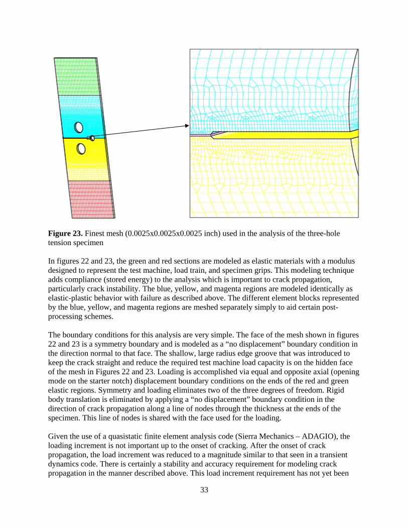
Figure 23. Finest mesh (0.0025x0.0025x0.0025 inch) used in the analysis of the three-hole tension specimen In figures 22 and 23, the green and red sections are modeled as elastic materials with a modulus designed to represent the test machine, load train, and specimen grips. This modeling technique adds compliance (stored energy) to the analysis which is important to crack propagation, particularly crack instability. The blue, yellow, and magenta regions are modeled identically as elastic-plastic behavior with failure as described above. The different element blocks represented by the blue, yellow, and magenta regions are meshed separately simply to aid certain post-processing schemes. The boundary conditions for this analysis are very simple. The face of the mesh shown in figures 22 and 23 is a symmetry boundary and is modeled as a “no displacement” boundary condition in the direction normal to that face. The shallow, large radius edge groove that was introduced to keep the crack straight and reduce the required test machine load capacity is on the hidden face of the mesh in Figures 22 and 23. Loading is accomplished via equal and opposite axial (opening mode on the starter notch) displacement boundary conditions on the ends of the red and green elastic regions. Symmetry and loading eliminates two of the three degrees of freedom. Rigid body translation is eliminated by applying a “no displacement” boundary condition in the direction of crack propagation along a line of nodes through the thickness at the ends of the specimen. This line of nodes is shared with the face used for the loading. Given the use of a quasistatic finite element analysis code (Sierra Mechanics – ADAGIO), the loading increment is not important up to the onset of cracking. After the onset of crack propagation, the load increment was reduced to a magnitude similar to that seen in a transient dynamics code. There is certainly a stability and accuracy requirement for modeling crack propagation in the manner described above. This load increment requirement has not yet been

34

established in a general sense. For the three-hole tension analyses described here, the load increment was established by a series of reductions in magnitude in the analysis of the finest mesh until no change was seen in the results. The load increment resulting from that study was then used throughout the remainder of the analyses. No estimate of the critical crack opening strain parameter was available. Therefore, this set of three-hole tension experiments was used to develop such an estimate. For each finite element mesh, a series of analyses was performed varying the critical crack opening strain parameter until the analysis was in reasonable agreement with the experimental results. This procedure was repeated for each of the three materials tested. This served three purposes. First, it showed that the failure criterion, energy dissipation scheme described in this report could match the experimental result for a specimen that exhibited significant stable crack growth. Second, it provided a demonstration that the energy dissipation technique proposed here could provide an element size independent result for crack propagation. Finally, it provided data for developing an element size to critical crack opening strain relationship that would provide for element size independent crack propagation simulation. The comparisons between the load-line displacement (LVDT measurement) versus the applied load for the experiment and the simulation are shown in figure 24 for the 304L stainless steel, in figure 25 for the 17-4PH stainless steel, and in figure 26 for the 6061-T6 aluminum. As discussed above, these comparisons shown must be considered “tuning” results in that the “critical crack opening displacement” (energy dissipation) parameter was adjusted to produce a simulation result that best matched the experiment.

Figure 24. Comparison between experimental and simulation results of load versus displacement for 304L stainless steel 3-hole tension

35

Figure 25. Comparison between experimental and simulation results of load versus displacement for 17-4PH stainless steel 3-hole tension

Figure 26. Comparison between experimental and simulation results of load versus displacement for 6061-T6 aluminum 3-hole tension

36

Figure 27. Comparison between experimental and simulation results of crack extension versus displacement for 304 stainless steel 3-hole tension

Figure 28. Comparison between experimental and simulation results of crack extension versus displacement for 17-4PH stainless steel 3-hole tension

37

Figure 29. Comparison between experimental and simulation results of crack extension versus displacement for 6061-T6 aluminum 3-hole tension In figures 24 through 29 the first dimension in the legend refers to the in-plane element dimension. The second dimension in the legend refers to the out-of-plane, or crack opening direction dimension. It is the element dimension in the crack-opening direction that is most important in controlling the necessary value for the critical crack opening strain. The in-plane, or more specifically the element dimension in the direction of crack extension has a smaller effect on the required value of critical crack opening strain. The element dimension along the crack front had no discernable effect on the required value of critical crack opening strain. The data shown in figures 24 through 26 were used to develop the critical crack opening strain (energy dissipation) parameter estimation scheme discussed in the parameter estimation section earlier in this report. Table 1 presents the critical crack opening displacement as a function of element dimensions and materials and compares the values derived from simulation of the three-hole tension specimens with the values from the estimation scheme. For this study, element dimensions were restricted to give no worse than a 4 to 1 aspect ratio (the generally expected limit of accuracy for this element type). In addition, for elements smaller than the smallest used in this study, compute resource requirements (number of processors and run times) became excessive. The 0.0025 by 0.0025 by 0.0025 inch elements became a practical lower bound on element size. The crack extension comparisons shown in figures 27 through 29 were not used in the establishment of the “correct” value for the critical crack opening displacement. They are included simply for completeness. There is a large uncertainty in the experimental determination

38

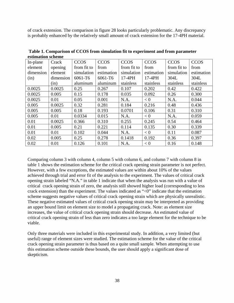
of crack extension. The comparison in figure 28 looks particularly problematic. Any discrepancy is probably enhanced by the relatively small amount of crack extension for the 17-4PH material. Table 1. Comparison of CCOS from simulation fit to experiment and from parameter estimation scheme In-plane element dimension (in)

Crack opening element dimension (in)

CCOS from fit to simulation 6061-T6 aluminum

CCOS from estimation 6061-T6 aluminum

CCOS from fit to simulation 17-4PH stainless

CCOS from estimation 17-4PH stainless

CCOS from fit to simulation 304L stainless

CCOS from estimation 304L stainless

0.0025 0.0025 0.25 0.267 0.107 0.202 0.42 0.422 0.0025 0.005 0.15 0.178 0.035 0.092 0.26 0.300 0.0025 0.01 0.05 0.001 N.A. < 0 N.A. 0.044 0.005 0.0025 0.32 0.281 0.184 0.216 0.48 0.436 0.005 0.005 0.18 0.193 0.0701 0.106 0.31 0.310 0.005 0.01 0.0334 0.015 N.A. < 0 N.A. 0.059 0.01 0.0025 0.366 0.310 0.255 0.245 0.54 0.464 0.01 0.005 0.21 0.221 0.114 0.135 0.30 0.339 0.01 0.01 0.102 0.044 N.A. < 0 0.11 0.087 0.02 0.005 0.25 0.278 0.1418 0.192 0.36 0.397 0.02 0.01 0.126 0.101 N.A. < 0 0.16 0.148 Comparing column 3 with column 4, column 5 with column 6, and column 7 with column 8 in table 1 shows the estimation scheme for the critical crack opening strain parameter is not perfect. However, with a few exceptions, the estimated values are within about 10% of the values achieved through trial and error fit of the analysis to the experiment. The values of critical crack opening strain labeled “N.A.” in table 1 indicate that when the analysis was run with a value of critical crack opening strain of zero, the analysis still showed higher load (corresponding to less crack extension) than the experiment. The values indicated as “<0” indicate that the estimation scheme suggests negative values of critical crack opening strain which are physically unrealistic. These negative estimated values of critical crack opening strain may be interpreted as providing an upper bound limit on element size to model a propagating crack. Note: as element size increases, the value of critical crack opening strain should decrease. An estimated value of critical crack opening strain of less than zero indicates a too large element for the technique to be viable. Only three materials were included in this experimental study. In addition, a very limited (but useful) range of element sizes were studied. The estimation scheme for the value of the critical crack opening strain parameter is thus based on a quite small sample. When attempting to use this estimation scheme outside these bounds, the user should apply a significant dose of skepticism.

39

EXAMPLES In 2010, a project was initiated to provide a snapshot in time of the current ability to model ductile failure (both initiation and propagation) in the Sierra Mechanics suite of codes. Four separate techniques (tearing parameter, localization elements, X-FEM, and peridynamics) were chosen for this study. This study was referred to (tongue-in-cheek) as the Ductile Failure X-Prize[30]. Only a very limited discussion of this project as it relates to the tearing parameter results will be presented here. The first challenge (challenge 1-A) of the Ductile Failure X-Prize project consisted of prediction of crack initiation from key-hole compact specimen with a kinked slot. The geometry of the specimen is shown in Figure 30. The specimens were made from a PH13-8Mo stainless steel which was heat treated to the H950 condition. There were eight nominally identical tests run. Crack initiation was determined by the operator viewing the specimen through a low power microscope. The tests were stopped after the initiation of a crack was detected. Both load and clip-gage displacement were recorded during the test.

Figure 30. Drawing of the challenge 1-A compact specimen with kinked-slot key-hole. A series of twelve analyses were run to bound the numerical results for challenge 1-A. These consisted of high and low material properties. The low material property set was extracted from a full stress-strain curve from the MIL handbook [31]. The high properties were extracted from one of a series of tensile tests conducted at Sandia in the 1990’s for a different project. This first X-prize challenge was started before the critical crack opening strain estimation scheme had been developed. Therefore, two values of critical crack opening strain (0.1 and 0.2) were rather arbitrarily selected the analyses employing the coarsest mesh. Two further levels of mesh

40

refinement (for a total of three different meshes) were used with the value of the critical crack opening strain adjusted for element size according to the equation by Foulk, shown earlier in this report. These analysis differences account for the variation in simulation results shown in Figure 31, which compares the experimental load versus the clip-gage displacement for the challenge 1-A specimen.

Figure 31. Comparison of experiment to simulation for load versus displacement for the ductile failure X-prize challenge 1-A. In addition to the variation in load versus displacement curves for the analyses discussed above, there is an additional source of uncertainty in the analytical clip-gage displacement at crack initiation. Crack initiation could reasonably be assumed in the analysis when the tearing parameter is exceeded or alternately when the stress has been decayed to zero. These two assumptions provide a significant variation in the clip-gage displacement at crack initiation. The experimental clip-gage displacement at failure varies between 0.1062 and 0.1220 inches compared to the simulation results, which include all sources of variation and uncertainty discussed above, at between 0.0945 and 0.1614 inches. The agreement between experiment and simulation is reasonable. The second x-prize challenge (challenge 1-B) consisted of prediction of both initiation and propagation. The specimen geometry was identical to that of challenge 1-A (see figure 28). For challenge 1-B a 2024-T3 aluminum alloy was chosen. One set of material properties was obtained from the MIL handbook [31]. Experimental yield, ultimate, and elongation values were

41

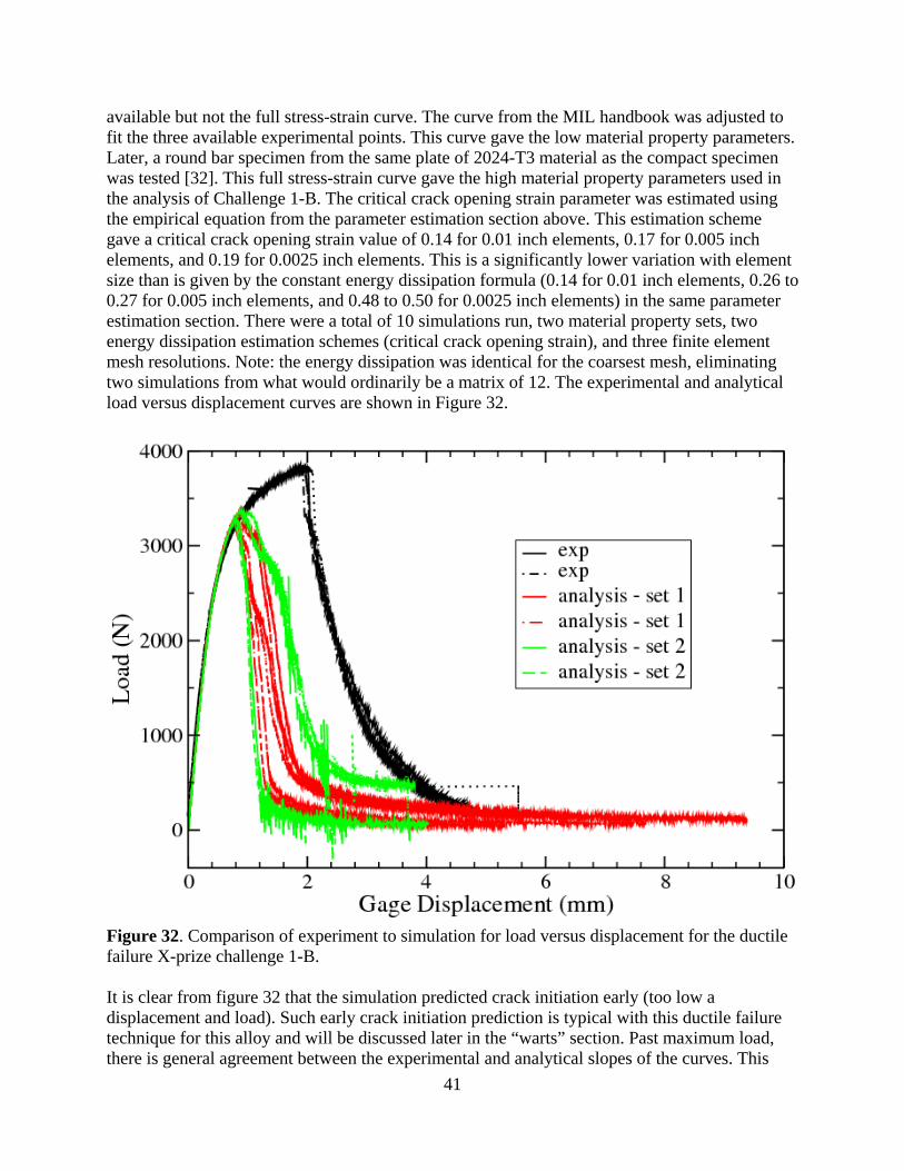
available but not the full stress-strain curve. The curve from the MIL handbook was adjusted to fit the three available experimental points. This curve gave the low material property parameters. Later, a round bar specimen from the same plate of 2024-T3 material as the compact specimen was tested [32]. This full stress-strain curve gave the high material property parameters used in the analysis of Challenge 1-B. The critical crack opening strain parameter was estimated using the empirical equation from the parameter estimation section above. This estimation scheme gave a critical crack opening strain value of 0.14 for 0.01 inch elements, 0.17 for 0.005 inch elements, and 0.19 for 0.0025 inch elements. This is a significantly lower variation with element size than is given by the constant energy dissipation formula (0.14 for 0.01 inch elements, 0.26 to 0.27 for 0.005 inch elements, and 0.48 to 0.50 for 0.0025 inch elements) in the same parameter estimation section. There were a total of 10 simulations run, two material property sets, two energy dissipation estimation schemes (critical crack opening strain), and three finite element mesh resolutions. Note: the energy dissipation was identical for the coarsest mesh, eliminating two simulations from what would ordinarily be a matrix of 12. The experimental and analytical load versus displacement curves are shown in Figure 32.

Figure 32. Comparison of experiment to simulation for load versus displacement for the ductile failure X-prize challenge 1-B. It is clear from figure 32 that the simulation predicted crack initiation early (too low a displacement and load). Such early crack initiation prediction is typical with this ductile failure technique for this alloy and will be discussed later in the “warts” section. Past maximum load, there is general agreement between the experimental and analytical slopes of the curves. This

42

indicates that the propagation behavior of the simulation is in reasonable agreement with the experiment. The final deformed shapes (after crack propagation) between the experiment and the simulation are compared in figure 33. Figure 33 indicates the simulation produces a crack path in good agreement with the experiment.

Figure 33. Comparison of experiment to simulation for deformed shape and crack path for the ductile failure X-prize challenge 1-B; left hand side is the experiment, right hand side is the pre-test analysis. The tearing parameter technique has also been used for another project, the “pipe-bomb” project which is currently underway. [33,34,35]. We have an application where an enclosed region filled with an organic compound (foam) is subjected to an external heat source (fire). The organic material will begin to degrade and release gasses upon reaching a sufficiently high temperature, thus causing pressurization of the enclosure. It is necessary to characterize the behavior of this enclosure up to and including breach. The purpose of this project is to assess the accuracy of simulation technique. A simplified geometry (a cylinder approximately 3.5 inch diameter by 14 inch long) was heated on one side via thermal radiation from an Inconel panel approximately 1 inch from the side wall. The Inconel panel was controlled to give the desired peak temperature (500 to 1000 degrees Centigrade depending on the test) on the wall of the pipe-bomb. This generated a complex temperature environment with a hot spot on one wall. An array of 28 thermocouples, surface mounted on the cylinder outside diameter, was used to sample the imposed temperature field, with one thermocouple used to provide feedback to the Inconel panel temperature controller. To simplify the boundary conditions, the cylinder was pressurized with nitrogen from a remote source. Data collection consisted of video recording of deformations during the test, as well as temperature at each thermocouple location and pressure as a function of time. The primary parameter was time to burst. The internally pressurized cylinder of the pipe-bomb can be considered a load controlled experiment. We are employing a quasistatic finite element analysis where each time step is converged to global equilibrium. Once the tensile instability (necking) is encountered in the pipe-

43

bomb wall, there is no longer an equilibrium state to be found. The tensile instability occurs prior to initiation of a ductile tear. Thus, the pipe-bomb primarily serves to investigate the accuracy of the large strain plasticity behavior in the finite element simulation. That is, in the simulation, failure pressure is defined by the inability of the simulation to converge. The temperature and pressure ramp employed in the testing requires approximately 20 minutes to burst the pipe-bomb. An adaptive time step in the analysis was truncated at a value of 1.E-09 seconds, representing an infinitesimal load increment. A typical quasistatic solution, just prior to the instability, is shown in Figure 34. The temperature field interpolated from experimental thermocouple data is shown in Figure 34-a. The “pinch” in the middle of the hot spot is an artifact of the spline interpolation scheme used and is not considered significant to the solution. The plastic strains produced by the combination of temperature and internal pressure is shown in Figure 34-b. Finally, the pipe-bomb is rotated 90 degrees on its long axis to show the bulge in the wall under the hot spot, just prior to failure in Figure 34-c.

Figure 34. Typical results from the quasistatic analysis of the “pipe-bomb” specimen just prior instability and failure; a) Temperature in degrees Kelvin, b) plastic strain, c) depiction of pre-failure bulge. To check that lack of code convergence was truly indicative of imminent pipe burst, several simulations were transferred over to a transient dynamics solution scheme where inertial terms stabilized the solution sufficiently that the failure technique was activated. In all such simulations, tearing was initiated and travelled axially the length of the thin walled test section. At the location where the wall thickness increased, the running crack changed direction and traveled around the specimen in the hoop direction. Both initiation and propagation occurred within milliseconds of the transfer to the transient dynamics scheme. The simulated failure pressures were higher than the experimental values by 10 to 30 per cent. Investigations of the effects of mesh refinement and initial aspect ratio of the elements on the burst pressure is

Temperature Degrees K

Plastic Strain

44

underway. The final deformed shape of the pipe-bomb, after burst, is compared to the simulation in Figure 35.

Figure 35. Comparison of experiment to simulation for deformed shape of the pipe-bomb after burst. Experiment on the left hand side, Analysis on the right hand side. WARTS Mesh line sensitivity For the most commonly used element type (8-node uniform gradient hex with a single integration point) the crack propagation path for the ductile failure technique discussed here traverses from one element centroid to another. This is a feature of performing all calculations at the integration point which is essentially located at the element centroid. As such, if the crack propagation direction is aligned from corner to corner of an element the numerical path will be longer than the actual path, leading to effectively retardation of crack propagation. This could be mitigated by adjusting the critical crack opening strain parameter (energy dissipation term). However, if the desire is to provide a predictive capability, such tuning of the energy dissipation is not possible at this time. We are currently working on automatic adjustment of the energy dissipation based on element size. In theory, such an adjustment could be made on element orientation as well. However, there are no current plans to explore this. Another mitigating factor is that typical meshing practice often produce elements aligned with principal stresses. Experience with this method has shown that another feature of mesh line sensitivity, difficulty in turning a corner to follow a changing load path, is not apparent. Curved crack propagation paths are readily achieved with this technique. The crack path maintains a direction perpendicular to the direction of the maximum principal strain. Given the current state of crack propagation using this methodology, mesh line sensitivity is inherent. Time/load step limitations There are stability and accuracy limits on the size of the load step that may be employed using this crack propagation methodology described in this report. Two manifestations of instability have been observed in practice. The first manifestation is element inversion which leads to the termination of solution. It has not been determined whether element inversion is an aspect of a fundamental instability or if it is a lack of robustness in the solvers used in the SIERRA

45

mechanics suite of codes. In either case, reduction in the load step size and in the artificial hourglass mode suppression has been beneficial in almost all cases. The second manifestation is in unstable crack propagation characterized by extensive cracking and failure to converge (inability to find an equilibrium state) in a single load increment. Both errors in crack propagation rate and in propagation direction have been observed. This is clearly related to the accuracy of computing the energy dissipation. In the SIERRA suite of codes, stress, strain, constitutive model variables (state variables), etc. are linearized over each load increment. If too large an increment is taken, the energy dissipated in computational failure of an element can be much too small. Figure 36 provides a graphical explanation of this phenomenon.

Figure 36. Potential effect of load increment on accuracy of energy dissipation No a priori assessment of a stable or accurate load step increment has been developed. Such stability criteria are under investigation. Load steps increments similar to the stable time step requirement (Courant limit) of transient dynamics solutions have been used with great success. This appears to be a safe (but probably expensive) estimate of an acceptable load increment to use with a quasistatic solution. At the current state of this modeling technique, the selection of an appropriate load step increment is left to the user. Solver robustness There are some issues with solver robustness. The dynamic relaxation solver, available in the legacy codes, proved to be the most robust of the solver techniques for ductile failure modeling. Dynamic relaxation has not been implemented in the SIERRA mechanics suite of codes. Currently, the FETI solver (SIERRA mechanics implementation that looks like a parallel direct solver) does not perform adequately with this approach to ductile failure. FETI appears to run into trouble when the element enters the stress decay portion of the failure process. This is not too surprising in that the element has a negative stiffness in this region. There are several

46

techniques that have been implemented (with mixed success) to attempt to mitigate this problem (diagonal scaling, diagonal shift, etc). The nonlinear conjugate gradient iterative solver has proven to be the most successful solver within the SIERRA mechanics suite of codes. This solver’s performance has been incrementally improved over the past several years to the point where its behavior is normally adequate. There are two major solver settings that have given the best results in the past. These are setting the line search parameter to “linear” and the preconditioner to “elastic”. For those special cases where the solver fails to converge, inverts an element, etc., relief can sometimes be obtained by reducing the load increment (less softening over a load step) or by reducing the hourglass suppression. This may seem counterintuitive, but for a softening element, the history involved with hourglass stiffness can cause, rather than prevent, hourglass deformations. Multiple integration point elements The current architecture in the SIERRA mechanics suite of codes lends itself to implementation of constitutive models integration point by integration point. This works wonderfully for the simple 8-node hex element with a single integration point. Higher order elements with multiple integration points can be more problematic. The behavior of most higher order elements becomes pathological when one or more integration points are passing through different paths of the constitutive model. One method to mitigate this problem would be to kill the element when one integration reaches the failure criterion. Unfortunately, this eliminated the energy dissipation portion of the failure model which is required to provide element size independent results. In addition, killing the element on one of many integration points leads to premature failure and too rapid crack propagation. Development of a compatible method to treat multiple integration points has not yet been successful but investigation is underway. Structural elements (shells) There is limited experience with shell elements and basically no experience with other structural elements (beam, membrane, etc.). The Key-Hoff shell implemented in SIERRA has a default value of five integration points through the thickness. At this default value, the shell will tolerate two to three integration points undergoing softening without pathological behavior. When the deformation is predominately membrane behavior, the shell is more likely to tolerate three integration points softening at a time. With a greater amount of bending deformation, reasonable element behavior is more likely to be achieved with two or fewer integration points undergoing softening. In almost every case, four integration points undergoing softening leads to bizarre deformations and element inversion. Therefore, it is recommended that the element be killed when three integration points remain. While the ductile failure model has been used with shell elements, there is little to no evidence that it gives correct answers. There is even less experience with other structural elements. 2024-T3 Aluminum The ductile failure techniques have been used with many materials with a good degree of success. However, recent work on 2024-T3 aluminum has shown a problem. The tearing parameter criterion predicts premature failure for this alloy. In fact, notched bar test results indicate no effect of hydrostatic (triaxial) tension on failure for this alloy. When the stress state exponent is reduced from its nominal value of four to zero, the failure model begins to reasonably predict failure of 2024-T3 aluminum. There is no explanation for this phenomenon. Observation suggests that 2024-T6 is the only alloy for which the failure model has been used

47

that exhibits failure prior to necking. That is, failure occurs on the rising portion of an engineering stress-strain curve. Whether this is a general limitation to the failure model applicability or it is specific to this alloy has not yet been determined. Because the failure model is dominated by plastic strain, it may not be surprising that this failure modeling technique does not lend itself well to relatively brittle behavior. Future testing and analysis using relatively brittle materials should be performed to further investigate this phenomenon. Shear There is currently no shear failure criterion implemented in the tearing parameter technique. It is believed that if the geometry and mesh are included in the analysis in fine enough detail, that nearly all shear failures are actually tensile in nature. A two dimensional (axisymmetric) analysis of a hole punching operation confirmed this premise for at least this one case. Here, because of the axisymmetric nature of the analysis, a sufficiently fine mesh could be applied to resolve the deformation of the workpiece around the radii of the punch and die. Failure initiated sub-surface where large tensile stresses were present in the workpiece adjacent to the relief cuts in the punch and die. However, such refinement is nearly always impractical in three dimensions. Therefore, investigation into appropriate shear failure criterion is underway. At the time of publication, no shear failure criterion has been selected. Energy dissipation No direct test for the energy dissipation (critical crack opening strain parameter) required during crack propagation exists. Energy dissipation during crack propagation should be based on material properties and adjusted based on element size. We have investigated two estimation schemes for adjusting the critical crack opening strain parameter to the initial element size, one theoretical and one empirical. The theoretical scheme appears to overstate the effect of mesh refinement. That is, as the mesh is refined, the increase in energy dissipation proposed by the theoretical scheme causes the simulated crack propagation to lag experimental observations. In addition, the theoretical scheme provides only an adjustment to the critical crack opening strain term based on element size. It does not provide a materials properties based starting point. In contrast, the empirical scheme provides a critical crack opening strain parameter based on material properties and element size. However, the empirical scheme is founded on only three materials and one test specimen. This limited basis argues for use of the empirical scheme with a great deal of caution and skepticism. For now, the best option is to perform a stable crack propagation test (like the three-hole tension test) and then run simulations, with varying mesh densities, adjusting the critical crack opening strain parameter until the simulation and experiment match. Unfortunately, it is unlikely that material, time or budget will be available for such a process. Thus, reliance on the empirical scheme will probably be required until a better approach is developed. A technique to control the critical crack opening strain parameter based on the current deformed size of the element has recently been implemented. This implementation is designed to provide a constant energy per unit area of new crack surface formed. That is, the strain energy density dissipated is adjusted based on the crack-opening dimension of the element to provide a constant energy dissipation. This technique is currently under review and assessment. CONCLUSIONS

48

A simple technique for modeling ductile failure initiation and propagation has been presented along with several cases demonstrating successful use. Guidance for using this technique including selection of model parameters has been described. Finally, limitations and suggestions for future improvements have been discussed. REFERENCES [1] Griffith, A. A., “The Phenomena of Rupture and Flaw in Solids”, Transactions, Royal Society of London, A221, 1920 [2] Barsom, J.M. and Rolfe, S. T., Fracture and Fatigue Control in Structures Applications of Fracture Mechanics, 2nd ed., Prentice-Hall, Inc, Englewood Cliffs, New Jersey, 1987. [3] Kanninen, M. F. and Popelar, C. H., Advanced Fracture Mechanics, Oxford University Press, New York, New York, 1985. [4] Owen, D. R. J., and Fawkes, A. J., Engineering Fracture Mechanics Numerical Methods and Applications, Pineridge Press Ltd., Swansea, U. K. 1983. [5] Newman, J. C., and Loss, F. J., eds., Elastic-Plastic Fracture Mechanics Technology, ASTM STP 896, American Society for Testing and Materials, Philadelphia, Pennsylvania, 1985. [6] Kachanov, L. M., “Time of the Rupture Process Under Creep Conditions”, Izvestiia Akademia Nauk, SSSR, 1958. [7] Krajcinovic, D., ”Continuum Damage Mechanics: When and How?”, International Journal of Damage Mechanics, 1995. [8] Krajcinovic, D., “Continuous Damage Mechanics Revisited: Basic Concepts and Definitions”, Journal of Applied Mechanics, 1985 [9] Krajcinovic, D., “Damage Mechanics: accomplishments, trends and needs”, International Journal of Solids and Structures, 2000. [10] Barenblatt, G. I., “The Mathematical Theory of Equilibrium Cracks in Brittle Fracture”, Advances in Applied Mechanics, Vol 7, Academic Press Inc. New York, N. Y., 1962. [11] Dugdale, D. S., “Yileding of Steel Sheets Containing Slits”, Journal of the Mechanics and Physics of Solids, 1960. [12] Tvergaard, V., “Crack Growth Predictions by Cohesive Zone Model for Ductile Fracture”, Journal of the Mechanics and Physics of Solids, 2001. [13] Tvergaard, V. and Hutchinson, J. W., “The Relation Between Crack Growth Resistance and Fracture Process Parameters in Elastic-Plastic Solids”, Journal of the Mechanics and Physics of Solids, 1992

49

[14] de Borst, R., “Computation of Post-Bifurcation and Post Failure Behavior of Strain-Softening Solids”, Computers and Structures, 1986. [15] de Borst, R., Remmers, J. J. C., and Needleman, A., “Mesh-independent Discrete numerical Representations of Cohesive-zone Models, Engineering Fracture Mechanics, 2005. [17] Wellman, G. W. and Salzbrenner, R. “Quasistatic Modeling and Testing of Exclusion Region Barrier Mock-Ups”, SAND92-0024, Sandia National Laboratories, Albuquerque, N. M., 1992. [18] Brozzo, P., Deluca, B. And Rendina, R., “A New Method for the Prediction of the Formability Limits of Metal Sheets”, Proceedings of the 7th Biennial Congress of International Deep Drawing Research Group, 1972. [19] Dawson, D.B., Antoun, B.R., and Mosher, D.A., “MAVEN Progress Report for FY98 Second Half”, Memo to distribution, Sandia National Laboratories, Livermore, California, October 5, 1998. [20] Dawson, D.B., Sangwook (Simon) Lee, and Lee, K.L., “Materials Characterization for the W80 Abnormal Mechanical V&V Milestone: Structural Alloys for WES Attachment”, SAND2005-6018 OUO, Sandia National Laboratories, Livermore, California, 2005. [21] Bazant, Zednek P. and Oh, B. H., “Crack Band Theory for Fracture of Concrete”, Materials and Structures 16, 1983. [22] de Borst, Rene, Remmers, Joris J. C., and Needleman, Alan, “Mesh-independent discrete numerical representations of cohesive-zone models”, Engineering Fracture Mechanics 17, 2006. [23] Stone, C. M., “Santos: A Two-Dimensional Finite Element Program for the Quasistatic Large Deformation, Inelastic Response of Solids, SAND90-0543, Sandia National Laboratories, Albuquerque, N. M., 1995. [24] Sierra Solid Mechanics Team, “Adagio 4.16 User’s Guide”, SAND2010-3111, Sandia National Laboratories, Albuquerque, N. M., 2010. [25] Shelton, T., Personal Communication and On-Line User Documentation, Sandia National Laboratories, Albuquerque, N. M., 2009. [26] Foulk, J., Personal Communication, Sandia National Laboratories, Livermore, N. M., 2010. [27] Newman, J. and Loss, F., eds., Elastic-Plastic Fracture Mechanics Technology, ASTM STP 896, American Society for Testing and Materials, Philadelphia, 1985. [28] Reu, P.L., Rogillio, B.R., and Wellman, G.W., “Crack Growth Measurement using Digital Image Correlation”, Experimental Analysis of Nano and Engineering Materials and Structures, 2007.

50

[29] Reu, P.L., Wellman, G.W., and Rogillio, B.R., “Stable Crack Growth Measurement using DIC as a Tool for Model Validation”, Proceedings SEM Annual Conference and Exposition on Experimental and Applied Mechanics, 2007. [30] Boyce, B.L., et.al. “Ductile Failure X-Prize”, SAND2011-????, Sandia National Laboratories, Albuquerque, N.M., 2011. [31] Military Handbook – Metallic Materials and Elements for Aerospace Vehicle Structures, MIL-HDBK-5E, Department of Defense, June, 1987. [32] Modern Industries, Inc., Materials Research Division, Certificate of Analysis Sample S-162606, EXCEL spreadsheet, Eire, Pennsylvania, July, 2010. [33] Dempsey, J.F., Wellman, G.W., Scherzinger, W.M., and Antoun, B.R., “Coupled Thermal Pressurization Failure with Verification”, SAND 2010-1123C, Proceedings of the ASME2010 International Mechanical Engineering Congress & Exposition, Vancouver, BC, Canada, Nov 11-18, 2010. [34] Antoun, B.R., Dempset, J.R., and Wellman, G.W., “Experiments and Predictions of Large Deformation and Failure in Thermo-mechanical Loading Environments”, SAND 2011-1807C, Proceedings of the 2011 SEM Annual Conference & Exposition on Experimental and Applied Mechanics, June 13-16, 2011, Uncasville, CT. [35] Romero, V., Dempsey, J.F., Wellman, G.W., Antoun, B.R., and Sherman, M., “Model Validation and UQ Techniques Applied to a Temperature Dependent Stainless-Steel Constitutive Model Tested on Heated Pipes Pressurized to Failure”, SAND-report in preparation, September 2011.

51

Distribution 1 MS0405 H. Duong 0432 1 MS1322 D. J. Littlewood 1444 1 MS0828 M. Pilch 1514 1 MS0836 A. B. Dodd 1514 1 MS3084 D. B. Dimos 1500 1 MS0557 D. M. Jones 1521 1 MS0386 C. C. O’Gorman 1522 1 MS0555 T. E. Cordova 1522 1 MS0613 T. J. Baca 1523 1 MS0372 H. E. Fang 1524 1 MS0372 N. L. Breivik 1524 1 MS0346 R. S. Chambers 1524 1 MS0372 E. Corona 1524 1 MS0824 J. Cox 1524 1 MS0346 B. Elisberg 1526 1 MS0372 J. M. Emery 1524 1 MS0372 J. Gorman 1524 1 MS0372 S. Grange 1524 1 MS0372 K. W. Gwinn 1524 1 MS0372 T. D. Hinnerichs 1524 1 MS0836 C. T. Key 1525 1 MS0372 J. Koester 1524 1 MS0372 C. S. Lo 1524 1 MS0372 K. N. Long 1524 1 MS0372 K. E. Metzinger 1524 1 MS0372 W. M. Scherzinger 1524 1 MS0840 J. M. Pott 1525 1 MS0840 J. G. Arguello 1525 1 MS0847 S. W. Attaway 1525 1 MS0840 M. M. Bailey 1525 1 MS0824 J. E. Bean 1525 1 MS0840 J. E. Bishop 1525 1 MS0836 D. A. Crawford 1525 1 MS0840 K. Dion 1525 1 MS0840 T. J. Fuller 1525 1 MS0372 J. D. Gruda 1525 1 MS0840 S. Haniff 1525 1 MS0836 E. N. Harstad 1525 1 MS0824 J. F. Holland 1525 1 MS0836 J. P. Korbin 1525 1 MS0840 D. B. Longcope 1525 1 MS0840 P. Newell 1525 1 MS0840 J. S. Rath 1525 1 MS0828 K. Ruggirello 1525

52

1 MS0836 R. G. Schmitt 1525 1 MS0836 S. C. Schumacher 1525 1 MS0836 J. S. Simmons 1525 1 MS0840 J. A. Smith 1525 1 MS0372 P. E. Specht 1525 1 MS0824 J. D. Sweetser 1525 1 MS0824 L. W. Tuttle 1525 1 MS0344 J. F. Dempsey 1526 1 MS0346 M. Neidigk 1526 1 MS1398 M. K. Neilsen 1526 1 MS0346 E. D. Reedy 1524 1 MS0372 D. Vangoethem 1526 1 MS0386 T. S. Edwards 1527 1 MS0380 J. Jung 1542 1 MS0380 M. K. Bhardwaj 1542 1 MS0380 N. K. Crane 1542 1 MS0380 G. J. Frias 1542 1 MS0380 J. E. Dolbow 1542 1 MS0380 M. W. Heinstein 1542 1 MS0380 K. D. Mish 1542 1 MS0380 K. H. Pierson 1542 1 MS0380 V. L. Porter 1542 1 MS0372 T. Shelton 1542 1 MS0380 J. D. Thomas 1542 1 MS0897 G. D. Sjaardema 1543 1 MS0110 K. F. Alvin 1220 1 MS0828 W. R. Witkowski 1544 1 MS0828 A. R. Black 1544 1 MS0386 K. J. Dowding 1544 1 MS0828 R. G. Hills 1544 1 MS0812 V. J. Romero 1544 1 MS0828 W. R. Witkowski 1544 1 MS0889 C. C. Battaile 1814 1 MS0889 T. E. Buchheit 1814 1 MS0889 B. Boyce 1831 1 MS0889 C. V. Robino 1831 1 MS0886 D. F. Susan 1831 1 MS0344 C. F. Briner 2626 1 MS1185 A. S. Gullerud 5417 1 MS0744 L. A. Akin 6233 1 MS0744 D. C. Harding 6233 1 MS1135 J. P. Petti 1534 1 MS0718 D. J. Ammerman 6234 1 MS9042 B. R. Antoun 8256 1 MS9042 J. W. Foulk 8256 1 MS9042 W. Y. Lu 8256 1 MS9404 A. Mota 8256

53

1 MS9042 J. Ostien 8256 1 MS9042 M. L. Chiesa 8259 1 MS9042 J. J. Dike 8259 1 MS9042 B. L. Kistler 8259 1 MS0840 Gerald Wellman 1527 1 MS0899 Technical Library 9536 (electronic copy)