A Simple Analysis of the Effect of Construction Materials on Bridge Impact Factors

M.L. Peterson

Chin-Gwo Chiou R. M. Gutkowski

Department of Civil Engineering

Colorado State University Fort Collins, CO 80523

June 1999

ACKNOWLEDGEMENTS

The authors wish to extend their appreciation to Dr. Donald W. Radford for his guidance and

supervision during the preparation of this report. Grateful acknowledgement also is given to Dr. Xiao Bin

Le for his inspiring advice in this effort, to Colorado State University for the use of facilities and

resources as well as cost sharing funds that were provided as a part of the MPC process and funding.

DISCLAIMER

The contents of this report reflect the views of the authors, who are responsible for the facts and

the accuracy of the information presented. This document is disseminated under the sponsorship of the

Department of Transportation, University Transportation Centers Program, in the interest of information

exchange. The U.S. Government assumes no liability for the contents or us thereof.

TABLE OF CONTENTS

1. Introduction ...................................................................................................................................1

Overview.................................................................................................................................1

Definitions of Impact Factor......................................................................................................2

International Perspective of Impact Factor..................................................................................6

2. The System Modal and Examples ....................................................................................................8

Approach.................................................................................................................................8

Review of Lagrangian Dynamics ...............................................................................................8

Derivation of an Euler-Bernoulli Beam.................................................................................... 11

The System Model.................................................................................................................. 14

Numerical Examples............................................................................................................... 17

3. Discussion and Recommendation ................................................................................................... 21

Discussion ............................................................................................................................. 21

Recommendation.................................................................................................................... 23

References ....................................................................................................................................... 25

LIST OF TABLES

Table 3.1 Ratio of impact factor of bridges built of three materials normalized to concrete

design (each bridge design has different natural frequencies)....................................... 21

Table 3.2 Ratio of impact factor of bridges built of three materials normalized to concrete

design (bridge design altered to equivalent natural frequencies in all cases) .................. 21

Table 3.3 Impact factor according to international bridge design codes ....................................... 22

Table 3.4 Ratio of impact factor (from examples 1-3) ................................................................ 22

Table 3.5 Ratio of impact factor (from examples 4-6) ................................................................ 22

Table 3.6 Comparison of ratio of impact factor (from examples 4-6)........................................... 23

1

LIST OF FIGURES

1.1 Mid-Span Deflections Under a Moving Vehicle Load ...............................................................2

1.2 International Perspective of Impact Factor................................................................................7

2.1 Lagrange=s Equation ------ Notation ........................................................................................8

2.2 Free Body and Kinetic Energy Diagrams of a Simply Supported Beam.................................... 11

2.3 Average Impact Factor Versus Span Length for Three Materials (Examples 1-3) ...................... 19

2.4 Average Impact Factor Versus Frequency for Three Materials (Examples 4-6) ......................... 20

2

EXECUTIVE SUMMARY

This research considers the influence of different construction materials on the dynamic impact

factor of bridges. The general concept of the dynamic impact factor and typical evaluation methods are

reviewed. A comparison of bridge codes from some countries is made. Then, a simply supported Euler-

Bernoulli beam is used to evaluate influence of materials on the impact factor. A numerical example is

shown with a constant vehicle loading substituted into the model using three different materials for the

bridge system. Interesting results from the model suggest that the choice of construction material is a

secondary factor in the dynamic impact factor. A large number of other factors can be evaluated in the

same manner to determine which design parameters have the greatest influence on the dynamic impact

factor. The simple method for evaluation of changes in the dynamic impact factor is expected to be useful

to practitioners and students who are interested not only in the influence of material selection, but also on

the other factors, such as pavement roughness.

1

1. INTRODUCTION

Overview

When a bridge receives vehicle loading, the vehicle suspension will react to roadway roughness

by compression and extension of the suspension system. This oscillation creates wheel-axle forces that

exceed the static weight during the time the acceleration is downward, and reduces the static weight when

acceleration is upward. This phenomenon is referred to as “impact loading” or “dynamic loading,”

commonly expressed as a portion of the static axle loads. The influence of dynamic loading on bridge

loading usually is computed using the impact factor, also known as dynamic factor, or dynamic load

allowance. The AASHTO specifications use the term impact factor, which also will be used in this report

[1].

Impact factor is an important parameter in bridge design and evaluation. As the amount and

weight of moving vehicles on roadways increase, the dynamic loading to a bridge system also increases,

and in consequence, the impact factor becomes more important. Observations and measurements indicate

that the dynamic behavior of a bridge system is a function of three primary factors [2]:

dynamic properties of the vehicle (mass, suspension, axle configuration, tires, speed)

road roughness (approach, roadway, cracks, potholes, waves)

dynamic properties of the bridge structure (span, mass, support types, materials, geometry).

It has been well established that natural frequencies of a bridge system have the primary influence

on its dynamic response. Material properties are an essential determinant of the natural frequencies of a

bridge. The influence of material properties is a primary motivation for the research.

Many investigations have been made to evaluate the impact factor of bridges. Significantly less

effort has been focused on the effect of construction materials on the impact factor. Hence, the intent of

this paper is to focus on the influence of different materials on the impact factor. The outline of this paper

is that a simple model based on a Lagrangian formulation of the Euler-Bernoulli beam is presented to

2

estimate the impact factor. This work is described after a review of definitions related to impact factor and

a review of specifications related to bridge design codes. Finally, the accuracy of bridge design codes

related to specifications of the impact factor will be examined using numerical data.

Definition of Impact Factor

The concept of a dynamic impact factor has been used in the design of bridges for years.

Generally, it has been suggested that the impact factor is defined as the amount of force, expressed as a

fraction of the static force, by which dynamic force exceeds static force. However, there is no uniformity

in the manner by which this increment is calculated from test data. The different ways of calculating the

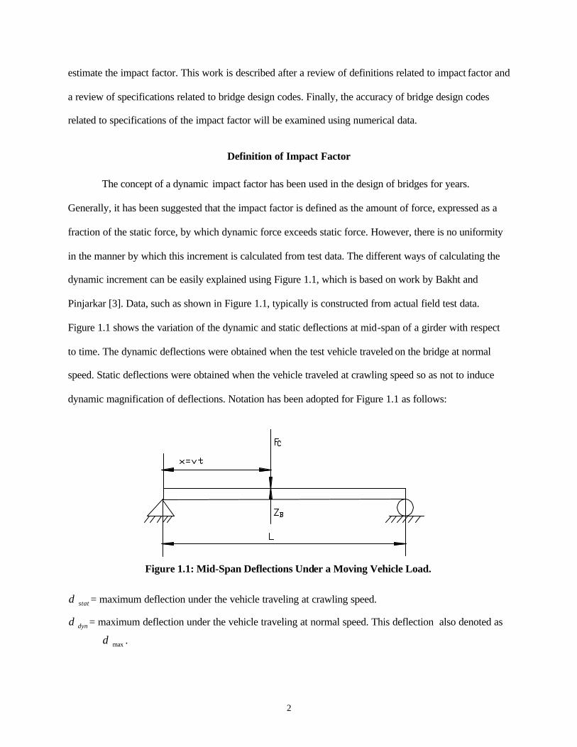
dynamic increment can be easily explained using Figure 1.1, which is based on work by Bakht and

Pinjarkar [3]. Data, such as shown in Figure 1.1, typically is constructed from actual field test data.

Figure 1.1 shows the variation of the dynamic and static deflections at mid-span of a girder with respect

to time. The dynamic deflections were obtained when the test vehicle traveled on the bridge at normal

speed. Static deflections were obtained when the vehicle traveled at crawling speed so as not to induce

dynamic magnification of deflections. Notation has been adopted for Figure 1.1 as follows:

Figure 1.1: Mid-Span Deflections Under a Moving Vehicle Load.

statδ = maximum deflection under the vehicle traveling at crawling speed.

dynδ = maximum deflection under the vehicle traveling at normal speed. This deflection also denoted as

maxδ .

3

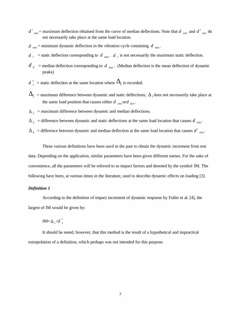
statδ ′ = maximum deflection obtained from the curve of median deflections. Note that statδ and statδ ′ do not necessarily take place at the same load location.

minδ = minimum dynamic deflection in the vibration cycle containing maxδ .

1δ = static deflection corresponding to maxδ . 1δ is not necessarily the maximum static deflection.

2δ = median deflection corresponding to maxδ . (Median deflection is the mean deflection of dynamic peaks)

*sδ = static deflection at the same location where 1∆ is recorded.

1∆ = maximum difference between dynamic and static deflections; 1∆ does not necessarily take place at

the same load position that causes either statδ or dynδ .

2∆ = maximum difference between dynamic and median deflections.

3∆ = difference between dynamic and static deflections at the same load location that causes statδ .

4∆ = difference between dynamic and median deflection at the same load location that causes statδ ′ .

These various definitions have been used in the past to obtain the dynamic increment from test

data. Depending on the application, similar parameters have been given different names. For the sake of

convenience, all the parameters will be referred to as impact factors and denoted by the symbol IM. The

following have been, at various times in the literature, used to describe dynamic effects on loading [3].

Definition 1

According to the definition of impact increment of dynamic response by Fuller et al. [4], the

largest of IM would be given by:

IM= 1∆ / *sδ

It should be noted, however, that this method is the result of a hypothetical and impractical

extrapolation of a definition, which perhaps was not intended for this purpose.

4

Definition 2

A commonly used variation of Definition 1 is that IM taken as the ratio of the measured

instantaneous dynamic response to the maximum static response. Thus,

IM= 3∆ / statδ

This definition has been used in most analytical studies.

Definition 3

When the static deflections are assumed to be the same as median deflections, Definition 2 of IM

changes to

IM= 4∆ / statδ ′

Definition 4

Definition 4 was used in Switzerland to interpret test data from the dynamic bridge tests

conducted from 1949 to 1965 [5]. According to this definition, the dynamic increment IM is given by

IM=minmax

minmax

δδδδ

+−

It is noted that this definition of the dynamic increment was abandoned in Switzerland after 1965

in favor of Definition 5.

Definition 5

According to the fifth definition, which has been used in Switzerland for tests conducted before

1945 and after 1965, the dynamic increment IM is given by

IM=2

2

δ

δδ −dyn

5

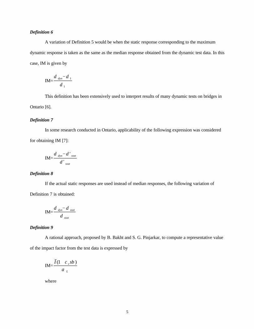
Definition 6

A variation of Definition 5 would be when the static response corresponding to the maximum

dynamic response is taken as the same as the median response obtained from the dynamic test data. In this

case, IM is given by

IM=1

1

δ

δδ −dyn

This definition has been extensively used to interpret results of many dynamic tests on bridges in

Ontario [6].

Definition 7

In some research conducted in Ontario, applicability of the following expression was considered

for obtaining IM [7]:

IM=stat

statdyn

δ

δδ

′

′−

Definition 8

If the actual static responses are used instead of median responses, the following variation of

Definition 7 is obtained:

IM=stat

statdyn

δ

δδ −

Definition 9

A rational approach, proposed by B. Bakht and S. G. Pinjarkar, to compute a representative value

of the impact factor from the test data is expressed by

IM=L

v scIα

β )1( +

where

6

I = mean value of the dynamic amplification factor [3];

vc = coefficient of variation of the dynamic amplification factor, that is , the ratio of standard deviation and mean;

s = the separation factor for dynamic loading, which has been found to have a value of 0.57 [3];

β = the safety index, from reliability based design, which typically has a value of about 3.5 for highway bridges; and

Lα = the live load factor

It is recommended that, in the absence of more rigorous analysis, the value of Lα should be taken

as 1.4 [3], which also is the live load factor specified in the Ontario Code [8].

The broad range of definitions of IM based on measured responses is a consequence of the facts

that, (a) the static response of a bridge is not necessarily the same as the median response obtained from

the dynamic test data, and (b) the maximum static and dynamic responses do not always take place under

the same load position. If the static and median responses were identical and the maximum static and

dynamic responses took place simultaneously, the diversity of definitions of IM would disappear and

Definitions 2 through 8 all would give the same value of IM for a given set of data [3].

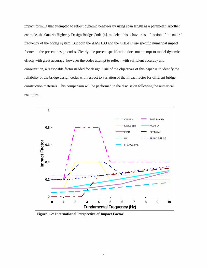
International Perspective of Impact Factor

Figure 1.2 shows various bridge engineering design specifications from around the world, which

use dramatically different factors [9]. The ordinate axis represents the load increase or impact factor and

the abscissa is the fundamental frequency of the structure. The broad variation indicates that the

international bridge design community has not yet reached a consensus about this issue. Figure 1.2 shows

bridge design specifications before 1992, more recent design codes of some countries also are included in

this paper since they have changed somewhat (AASHTO (USA) [1], OHBDC (Canada) [10], Highway

bridge design code (Taiwan) [11], and Eurocode (European) [12]). The AASHTO bridge design code and

OHBDC have been adopted by many countries. The Eurocode is accepted by most countries in the

European community. A tendency is shown, among recent design codes, that specific numerical impact

factors are used to replace formula based factors. For example, the previous AASHTO code [13] used an

7

impact formula that attempted to reflect dynamic behavior by using span length as a parameter. Another

example, the Ontario Highway Design Bridge Code [4], modeled this behavior as a function of the natural

frequency of the bridge system. But both the AASHTO and the OHBDC use specific numerical impact

factors in the present design codes. Clearly, the present specification does not attempt to model dynamic

effects with great accuracy, however the codes attempt to reflect, with sufficient accuracy and

conservation, a reasonable factor needed for design. One of the objectives of this paper is to identify the

reliability of the bridge design codes with respect to variation of the impact factor for different bridge

construction materials. This comparison will be performed in the discussion following the numerical

examples.

Figure 1.2: International Perspective of Impact Factor

0

0.2

0.4

0.6

0.8

1

0 1 2 3 4 5 6 7 8 9 10

Fundamental Frequency (Hz)

Impa

ct F

acto

r

CANADA SWISS vehicle

SWISS lane AASHTO

INDIA GERMANY

U.K. FRANCE d/l=0.5

FRANCE d/l=5

8

2. THE SYSTEM MODEL AND EXAMPLES

Approach

The approach taken in this study was to develop a small analytical model that can be used to

explore the sensitivity of bridge dynamic impact factors to a number of input variables. The initial model

uses a simply-supported Euler-Bernoulli beam to approximate response of the bridge span. The outline of

the approach is such that the derivations using the Lagrangian formulation of the Euler-Bernoulli (E-B)

beam assumptions are appropriately reviewed first. Next, the model shape function of the system are

found. Finally, the formula which determines deflection induced by a loading force at any location in the

E-B beam is presented. After this development, numerical examples are generated. The purpose of this

effort is to provide an overview of impact factors using a simple model system. This provides a

foundation for which an improved model can be incorporated into subsequent phases of the study.

Review of Lagrangian Dynamics

Lagrange’s equation, which is based upon energy concepts, is an extremely powerful device for

analysis of dynamic systems. To develop this foundation and to make it match the assumptions associated

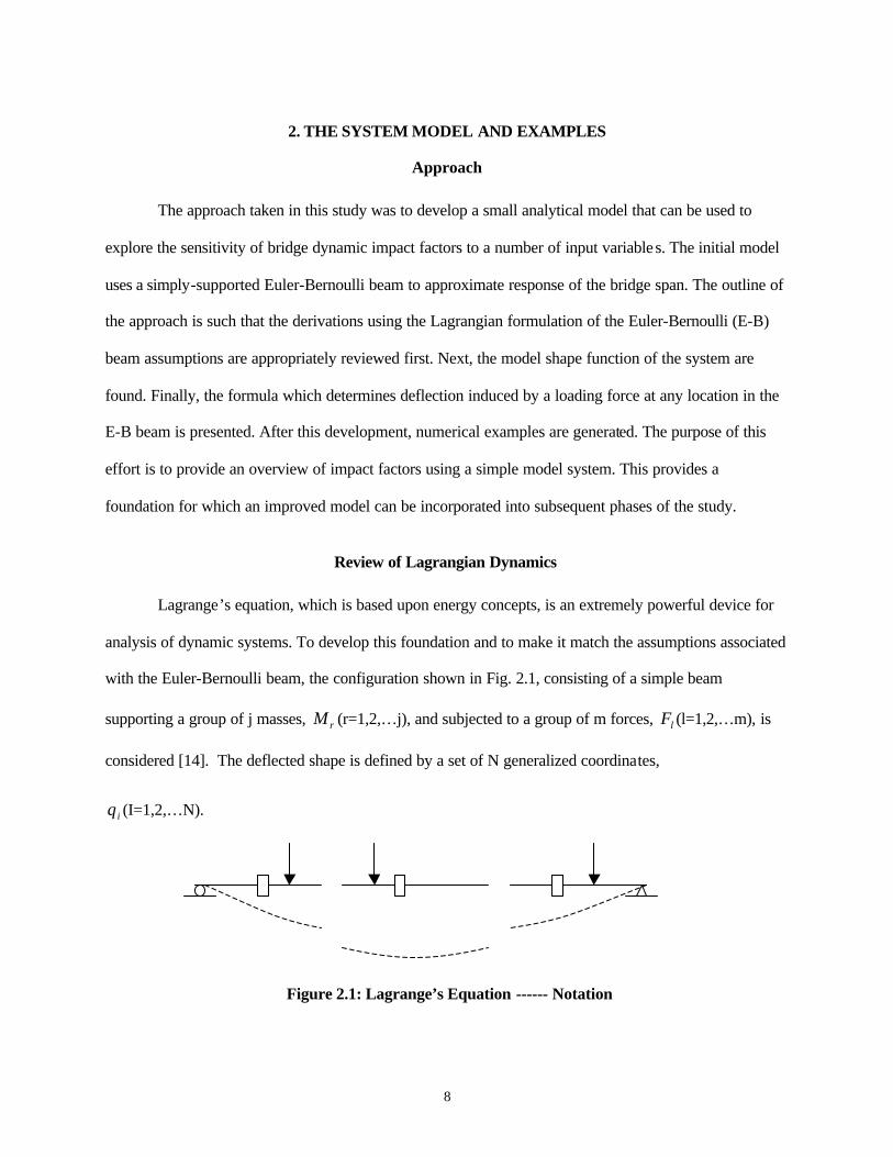
with the Euler-Bernoulli beam, the configuration shown in Fig. 2.1, consisting of a simple beam

supporting a group of j masses, rM (r=1,2,…j), and subjected to a group of m forces, lF (l=1,2,…m), is

considered [14]. The deflected shape is defined by a set of N generalized coordinates,

iq (I=1,2,…N).

Figure 2.1: Lagrange’s Equation ------ Notation

9

Suppose now that a virtual displacement is introduced consisting of a small change in one

generalized coordinate, iq . Let this change be designated by iqδ . By the principle of virtual work, the

work done by external forces during the virtual disturbance must equal the corresponding change in

internal strain energy. We may write the preceding statement as

UWWW cine δδδδ =++ (2.1)

where

eWδ = virtual work done by external loads lF

inWδ = virtual work done by inertia forces

cWδ = virtual work done by damping forces

Uδ = change in internal strain energy

Three of these terms may be expressed simply as

ii

ee q

qW

W δδ∂∂

= (a)

ii

cc q

qW

W δδ∂∂

= (b) (2.2)

ii

qqU

U δδ∂∂

= (c)

and inWδ may be expressed by

ii

rr

j

rrin q

qy

yMW δδ∂∂′′−= ∑

=

)(1

where ry is the total displacement at mass r. inWδ also can be expressed in the equivalent form as

ii

rr

j

rri

i

rr

j

rrin q

qy

yMqqy

yMdtd

W δδδ∂

′∂′+∂∂′−= ∑∑

== 11

(2.3)

The equation shown in (2.3) is based upon the fact

i

rr

i

rr

i

rr q

yy

qy

yqy

ydtd

∂′∂′+

∂∂′′=

∂∂′ )(

10

Now, we define the kinetic energy K and its derivatives as

2

1 21

rr

j

r

yMK ′= ∑=

(a)

i

rr

j

rr

i qy

yMqK

′∂′∂′=

′∂∂ ∑

=1

(b) (2.4)

i

rr

j

rr

i qy

yMqK

∂′∂′=

∂∂ ∑

=1

(c)

Furthermore, since ry is a function of iq ,

ii

rr q

qy

y ′∂∂

=′ and i

r

i

r

qy

qy

∂∂

=′′

Equation (2.4b) may therefore, be rewritten as

i

rr

j

rr

i qy

yMqK

∂∂′=

′∂∂ ∑

=1

(2.5)

If then Eqs. (2.4c) and (2.5) are substituted into Eq. (2.3), the result has the form

ii

ii

in qqK

qqK

dtd

W δδδ )()(∂∂

+′∂

∂−= (2.6)

Finally, by substituting Eqs. (2.2) and (2.6) into Eq. (2.1) and canceling iqδ , equation (2.7) is

obtained

i

e

i

c

iii qW

qW

qU

qK

qK

dtd

∂∂

=∂∂

−∂∂

+∂∂

−′∂

∂)( (2.7)

Equation (2.7) shows the kinetic energy K, the strain energy U, the work done by the damping

forces cW , and the work done by real external forces eW in terms of the generalized coordinates 1q …

Nq . When these expressions are differentiated as indicated and substituted into Eq. (2.7), the result is an

equation of motion. In the case under consideration, the term iqK ∂∂ / is zero, since kinetic energy is a

function of velocity rather than of displacement. Hence, Lagrange’s equation becomes

11

i

e

i

c

ii qW

qW

qU

qK

dtd

∂∂

=∂∂

−∂∂

+′∂

∂)( (2.8)

Derivation of an Euler-Bernoulli (E-B) Beam

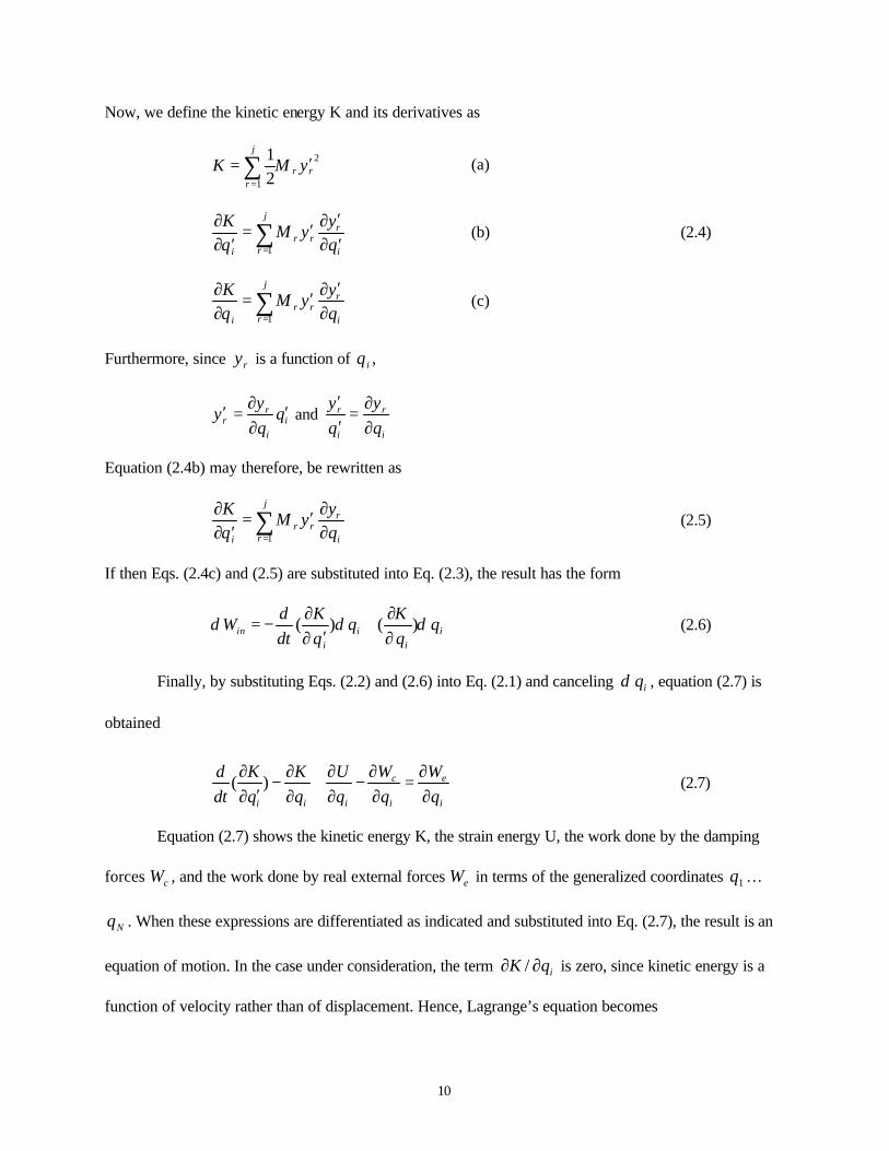
Assume a simply supported uniform beam with constant length (l), uniform distributed mass (m),

mass per length ( ρ ), and flexural rigidity (EI) as shown in Fig. 2.2. From a free body of the beam and

considering the influence of the kinetic energy, the equation of motion can be derived from Newton's

second law. Note that small displacements will be assumed (ds=dx).

F.B.D. y M+dM M V ds V+dV x dx K.E.D.

2

2

ty

dx∂∂

ρ

ρ = mass per length

Figure 2.2: Free Body and Kinetic Energy Diagrams of a Simply Supported Beam

Adding forces in the vertical direction, Newton's second law implies that

yy MaF =↑ ∑

From this addition it is then evident

2

2

]),([ty

dxdvdxtxf∂∂

=− ρ

The equation of motion could be expressed as

),(2

2

txfdxdv

ty

=+∂∂

ρ (2.9)

12

The shear and moment of a beam are

2

2

,dx

ydEIM

dxdM

v ==

which then produces from the second derivative

4

4

2

2

2

2

][x

yEI

xy

EIdxd

dxdv

∂∂

=∂∂

=

which is then substituted into (2.9), to arrive at

),(

4

4

2

2

txfxy

EIty

=∂∂

+∂∂

ρ (2.10)

To get the normal model shape, we set f(x,t)=0 and use separation of variables. Assume

)()(),( tTxXtxy = (2.11)

then substituted into (2.10) with f(x,t)=0, to arrive at

0)]()([)()]()([4

4

2

2

=+ tTxXx

EItTxX

t ∂∂

ρ∂∂

If set CTT

XXEI

=′′

=−""

)(ρ

(2.12)

then the two domains of a Euler-Bernoulli beam are

0)( "" =+ CXXEIρ

(mode shape) (2.13a)

0=−′′ CTT (time response) (2.13b)

To get the natural frequencies and the normal mode shapes of a E-B beam, we start with the

equation (2.13a). Since C=+ 2ω or C=0 gives no solution, we assume C=- 2ω . Then

0)(2

"" =−⇒ XEI

Xρω

If, for this case,

42

βρω

=EI

13

then, the resulting solution has the familiar form

)sin()cos()sinh()cosh()( xdxcxbxaxX ββββ +++=

The second derivative of the equation is

)sin()cos()sinh()cosh()( 2222" xdxcxbxaxX ββββββββ −−+=

Then it is necessary to impose boundary conditions as follows:

00)0( =+⇒= caX

0)sin()cos()sinh()cosh(0)( =+++⇒= ldlclblalX ββββ

0)0(" =−= caX

0)sin()cos()sinh()cosh()( 2222 =−−+=′′ ldlclblalX ββββββββ

0==⇒ ca

and

=−=+

0)sin()sinh(0)sin()sinh(

ldlbldlb

ββββ

0)sin()sinh(

)sin()sinh(=

−

⇒db

llll

ββββ

For a non-zero solution, the determinant of the matrix of the coefficients must equal zero. Then, it is

necessary to

0)sin()sinh(

)sin()sinh(=

− llll

ββββ

which has the result

0)sin()sinh(2 =−⇒ ll ββ

since 0)sinh( ≠lβ if 0≠lβ

0)sin( =⇒ lβ , and b=0

,....3,2,1,, ===⇒ nl

nnl nn

πβπβ

14

,....3,2,1,)(, 2242

====⇒ nEI

lnEI

EI nnnn

ρπ

ρβωβ

ρω

The solution for the shape function is then

)sin()sin()(l

xnxxX nn

πβ == (2.14)

This gives the familiar shape functions associated with the E-B beam.

The System Model

To determine the response of an E-B beam due to applied forces, the Lagrange's equation will be

used.

From Eq. (2.11)

)()(),(1

tTxXtxy nn

n∑∞

=

=

The velocity of the beam is then given by

)()(),(1

tTxXtxyn

nn∑∞

=

′=′

The kinetic energy of the complete system can be expressed as

dxtTxXdxyK n

l

nn

l 2

01

0

2 )]()([21

21 ′=′= ∫ ∑∫

∞

=

ρρ

Expanding the series, we arrive at

dxtTxXtTxXdxtTxXK mm

l

nnnn

l

nn )]()()][()([)]()([

21

01

2

01

2 ′′+′= ∫ ∑∫ ∑∞

=

∞

=

ρρ

The second term indicates the sum of all the modal cross products, which is equal to zero because of the

orthogonal condition of the shape function. Then

dxxXTdxtTxXKl

nn

nn

l

nn )(

21

)]()([21

0

2

1

22

01

2 ∫∑∫ ∑∞

=

∞

=

′=′= ρρ

and

15

dxxXTTK l

nnn

)(0

2∫′=′∂

∂ρ

dxxXTTK

dtd l

nnn

)(0

2∫′′=′∂

∂ρ

The work done by external forces during an arbitrary distortion is

dxtTxXxptFdxtTxXtxfW nn

n

l

n

l

nne )]()([)()()]()()[,(

100

1∑∫∫ ∑

∞

=

∞

=

== , if we set f(x,t)=F(t)p(x)

The rate of change of external work with respect to nT is therefore

dxxXxptFTW l

nn

e )()()(0∫=

∂∂

The internal strain energy is

dxXTEI

dxdx

ydEI

EIdx

EIM

U n

l

nn

ll 2

01

22

2

00

2

)(2

)(21

2′′=== ∫ ∑∫∫

∞

=

The rate of change of internal strain energy with respect to nT is therefore

dxXEITTU l

nnn

2

0)(∫ ′′=

∂∂

242 )()()(),sin( nnn Xl

nXx

ln

Xππ

=′′∴=Q

Then

dxXTl

nEI

TU l

nnn

2

0

4 )()( ∫=∂∂ π

Writing the Lagrange’s equation (2.8) with damping omitted and substituting from the above, we obtain

n

e

nn TW

TU

TK

dtd

∂∂

=∂∂

+′∂

∂

dxxXxptFdxXTl

nEIdxxXT

l

n

l

nn

l

nn )()()()()(00

24

0

2 ∫∫∫ =+′′ πρ (2.15)

16

Since we know by previous definition (Eq. (2.12)) that, if the last equation (2.15) is divided by the

coefficient of nT ′′ , the coefficient of nT becomes 2nω . Thus

∫∫

=+′′l

n

l

n

nnndxxX

dxxXxptFtTtT

0

2

02

)(

)()()()()(

ρω (2.16)

If damping is then added, equation (2.16) then becomes

∫∫

=+′+′′l

n

l

n

nnnnnndxxX

dxxXxptFtTtTtT

0

2

02

)(

)()()()()(2)(

ρωωξ (2.17)

In this paper, the focus is on the influence of construction materials on the theoretical value of the

impact factor. Hence, a relatively simple case of a constant force F moving across the span of a beam at

constant velocity v will be used.

From Eq. (2.14), the shape function has the form

)sin()(l

xnxX n

π=

Hence, the right-hand side of Eqs. (2.16) and (2.17) is replaced by

2/

)sin()(0

l

dxlxn

xpFl

ρ

π∫

where x is the distance from the end of the span to the force. Assume x is a function of time and is equal

to vt, where t is measured from the instant at which the force entered the span. After substitution of x=vt,

and p(x)=δ (x=vt) (δ function at x=vt, which means that p(x)=1 when x=0 and x=l, p(x)=0, otherwise),

Eqs. (2.16) and (2.17) become

)sin(2

)()( 2

lvtn

lF

tTtT nnnπ

ρω =+′′ (2.18)

)sin(2

)()(2)( 2

lvtn

lF

tTtTtT nnnnnnπ

ρωωξ =+′+′′ (2.19)

17

After imposing the initial conditions, y(x,0)=0 and y′ (x,0)=0, the solution of Eq. (2.18) is

)sin(sin12

)(22

ttl

FtT n

n

nn

nnn ω

ωωρΩ

−ΩΩ−

=

where lvnn /π=Ω . Since )()(),(1

tTxXtxy nn

n∑∞

=

= , we obtain the total solution for the deflection

)sin()sin(sin12

),(1

22 lxn

ttlF

txy nn

nn

n nnn

πω

ωωρΩ

−ΩΩ−

= ∑∞

=

If we assume viscous damping in each mode where where nnn ξωγ =/ is the fraction of critical damping

in the n-th mode, the solution then becomes

]sin)2(cos2[

cos2sin)()(4)(

)/sin(2),(

222

22

12222

tte

ttlxn

lF

txy

nnnnn

nnnn

t

nnnnnnn nnnn

n

n ωωγω

ωγ

γωγω

πρ

γ −Ω+Ω

+Ω+

ΩΩ−ΩΩ−Ω+Ω−

=

−

∞

=∑

(2.20)

which will be used as the governing equation of the system model in this research.

Numerical Examples

To evaluate the influence of construction materials on impact factors, three examples of bridges

by reinforced concrete, steel, and timber will be taken based on the information by Barker and Puckett

[15]. To get similar foundational characteristic for the bridges, three other examples with unique natural

frequencies will be shown. The dynamic deflection is calculated by the governing Eq. (2.20). And the

static deflection is based on the following formula,

])2

()([6

2/)( 222 lvtll

lEIlvtlF

ysta −−−−

= l/v ≤ t ≤ l/(2v)

EIvtlFl

vtlllEI

lvtlFysta 6

)2/(])

2()([

62/)( 3

222 −+−−−

−= 0 ≤ t ≤ l/(2v)

where

F: is the vehicle loading

l: is the span length of the bridge beam

18

v: is the velocity of the vehicle, and

t: is the time

Definition 8 of the impact factor using the static instead of the median displacement will be used

in the examples because definition 8 is used in the AASHTO code and the bridge examples are designed

based on the AASHTO code. For this case the impact factor is

IM=stat

statdyn

δδδ −

where

statδ = maximum static deflection

dynδ = maximum dynamic deflection

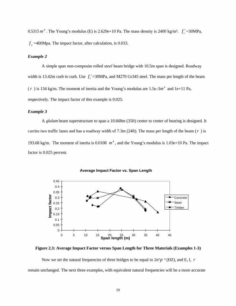
Calculations were performed using symbolic math in Maple and with Excel to process and plot

the results. The dynamic impact factors at mid-span are presented in Figs. 2.3-2.4. Figure 2.3 corresponds

to calculations obtained using examples 1-3 and Figure 2.4 corresponds to calculations obtained for

examples 4-6. The ratio analysis of the impact factor is discussed in a following section.

A constant vehicle loading (F=100KN) with a constant velocity (v=30mile/hr, 13.41m/sec) will

be assumed. An equivalent damping equal to 0.02 of critical damping (damping ratio ξ =0.02) also will

be presumed for all the examples. The examples will be calculated from information on bridges as

follows:

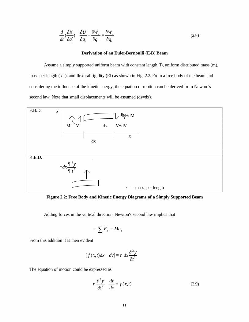
Example 1

A reinforced concrete T-beam bridge was designed for a 13.42m wide roadway and three-spans

of 10.67m-12.8m-10.67m with a skew of 30 degrees. The first span of 10.67m evaluates the impact

factor. The area of the T-beam (A) is 0.65475 m². The moment of inertia of the beam cross section (I) is

19

0.5315 4m . The Young’s modulus (E) is 2.629e+10 Pa. The mass density is 2400 kg/m³. cf ′ =30MPa,

yf =400Mpa. The impact factor, after calculation, is 0.033.

Example 2

A simple span non-composite rolled steel beam bridge with 10.5m span is designed. Roadway

width is 13.42m curb to curb. Use cf ′ =30MPa, and M270 Gr345 steel. The mass per length of the beam

( ρ ) is 134 kg/m. The moment of inertia and the Young’s modulus are 1.5e-3 4m and 1e+11 Pa,

respectively. The impact factor of this example is 0.025.

Example 3

A glulam beam superstructure to span a 10.668m (35ft) center to center of bearing is designed. It

carries two traffic lanes and has a roadway width of 7.3m (24ft). The mass per length of the beam (ρ ) is

193.68 kg/m. The moment of inertia is 0.0108 4m , and the Young’s modulus is 1.03e+10 Pa. The impact

factor is 0.025 percent.

Figure 2.3: Average Impact Factor versus Span Length for Three Materials (Examples 1-3)

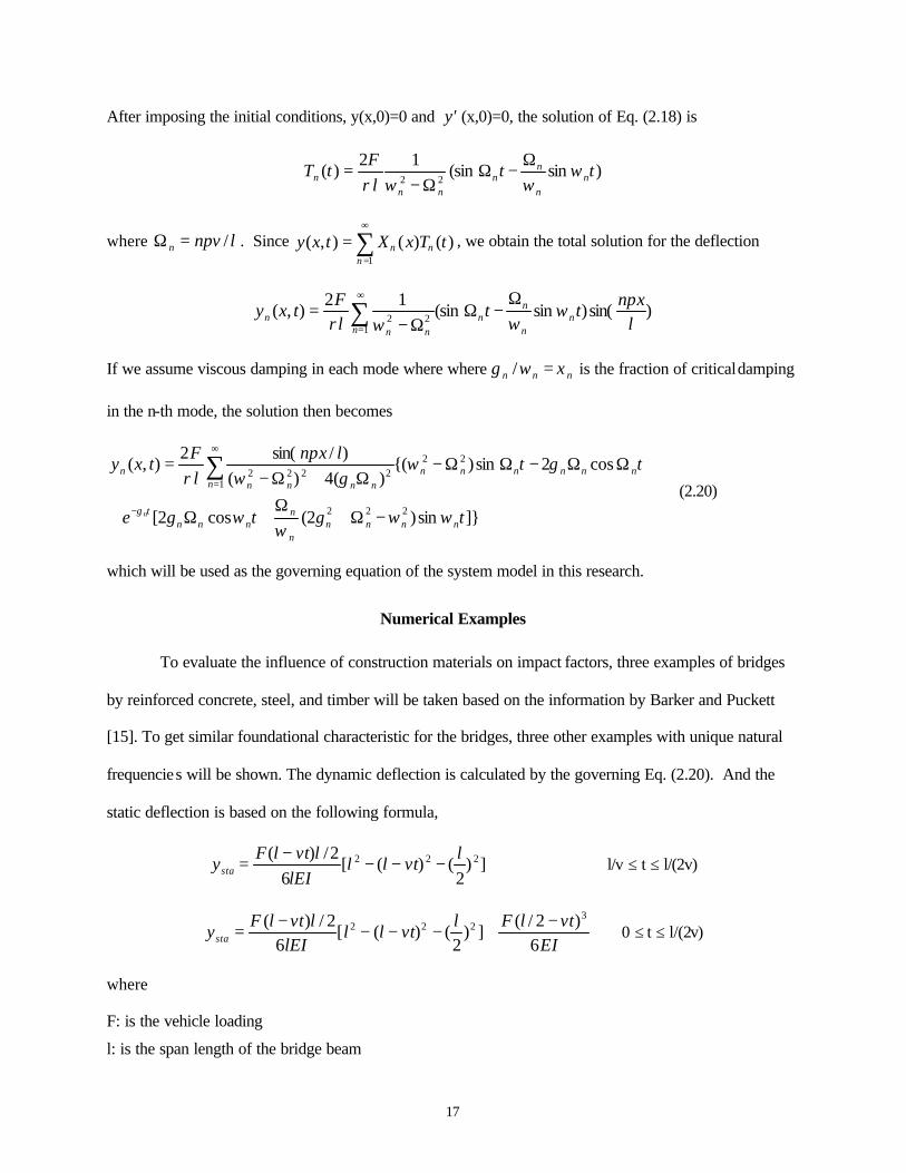
Now we set the natural frequencies of three bridges to be equal to 2n²π ² (HZ), and E, I, ρ

remain unchanged. The next three examples, with equivalent natural frequencies will be a more accurate

Average Impact Factor vs. Span Length

0

0.05

0.1

0.15

0.2

0.25

0.3

0.35

0.4

0.45

0 5 10 15 20 25 30 35 40 45Span length (m)

Impa

ct f

acto

r

Concrete

Steel

Timber

20

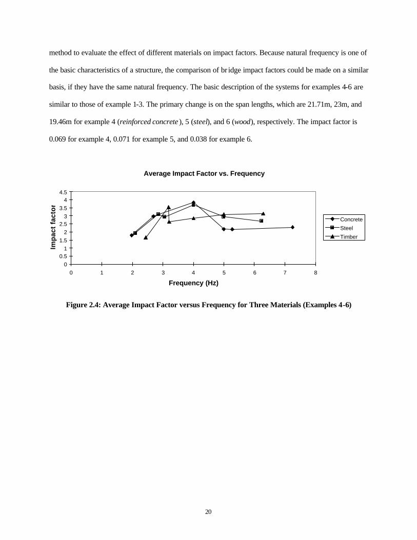
method to evaluate the effect of different materials on impact factors. Because natural frequency is one of

the basic characteristics of a structure, the comparison of br idge impact factors could be made on a similar

basis, if they have the same natural frequency. The basic description of the systems for examples 4-6 are

similar to those of example 1-3. The primary change is on the span lengths, which are 21.71m, 23m, and

19.46m for example 4 (reinforced concrete ), 5 (steel), and 6 (wood), respectively. The impact factor is

0.069 for example 4, 0.071 for example 5, and 0.038 for example 6.

Figure 2.4: Average Impact Factor versus Frequency for Three Materials (Examples 4-6)

Average Impact Factor vs. Frequency

00.5

11.5

22.5

33.5

44.5

0 1 2 3 4 5 6 7 8

Frequency (Hz)

Imp

act

fact

or

Concrete

Steel

Timber

21

3. DISCUSSION AND RECOMENDATION

Discussion

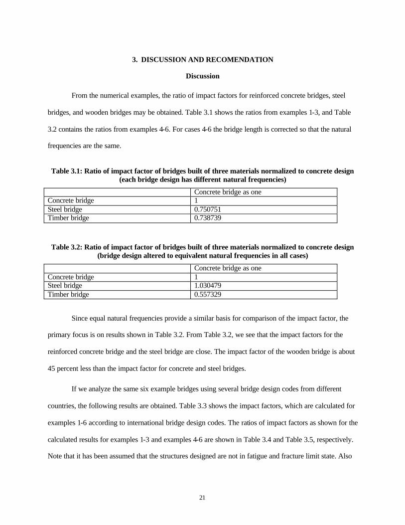
From the numerical examples, the ratio of impact factors for reinforced concrete bridges, steel

bridges, and wooden bridges may be obtained. Table 3.1 shows the ratios from examples 1-3, and Table

3.2 contains the ratios from examples 4-6. For cases 4-6 the bridge length is corrected so that the natural

frequencies are the same.

Table 3.1: Ratio of impact factor of bridges built of three materials normalized to concrete design (each bridge design has different natural frequencies)

Concrete bridge as one Concrete bridge 1 Steel bridge 0.750751 Timber bridge 0.738739

Table 3.2: Ratio of impact factor of bridges built of three materials normalized to concrete design (bridge design altered to equivalent natural frequencies in all cases)

Concrete bridge as one Concrete bridge 1 Steel bridge 1.030479 Timber bridge 0.557329

Since equal natural frequencies provide a similar basis for comparison of the impact factor, the

primary focus is on results shown in Table 3.2. From Table 3.2, we see that the impact factors for the

reinforced concrete bridge and the steel bridge are close. The impact factor of the wooden bridge is about

45 percent less than the impact factor for concrete and steel bridges.

If we analyze the same six example bridges using several bridge design codes from different

countries, the following results are obtained. Table 3.3 shows the impact factors, which are calculated for

examples 1-6 according to international bridge design codes. The ratios of impact factors as shown for the

calculated results for examples 1-3 and examples 4-6 are shown in Table 3.4 and Table 3.5, respectively.

Note that it has been assumed that the structures designed are not in fatigue and fracture limit state. Also

22

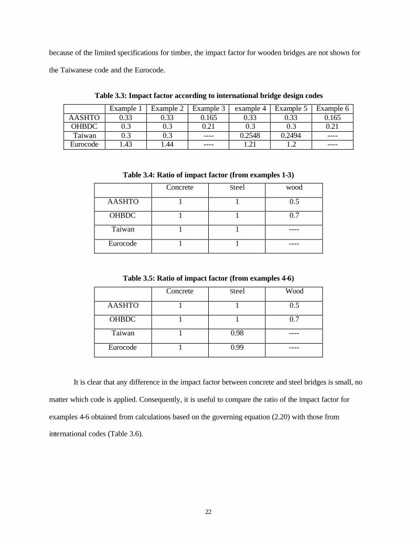
because of the limited specifications for timber, the impact factor for wooden bridges are not shown for

the Taiwanese code and the Eurocode.

Table 3.3: Impact factor according to international bridge design codes

Example 1 Example 2 Example 3 example 4 Example 5 Example 6 AASHTO 0.33 0.33 0.165 0.33 0.33 0.165 OHBDC 0.3 0.3 0.21 0.3 0.3 0.21 Taiwan 0.3 0.3 ---- 0.2548 0.2494 ----

Eurocode 1.43 1.44 ---- 1.21 1.2 ----

Table 3.4: Ratio of impact factor (from examples 1-3)

Concrete Steel wood

AASHTO 1 1 0.5

OHBDC 1 1 0.7

Taiwan 1 1 ----

Eurocode 1 1 ----

Table 3.5: Ratio of impact factor (from examples 4-6)

Concrete Steel Wood

AASHTO 1 1 0.5

OHBDC 1 1 0.7

Taiwan 1 0.98 ----

Eurocode 1 0.99 ----

It is clear that any difference in the impact factor between concrete and steel bridges is small, no

matter which code is applied. Consequently, it is useful to compare the ratio of the impact factor for

examples 4-6 obtained from calculations based on the governing equation (2.20) with those from

international codes (Table 3.6).

23

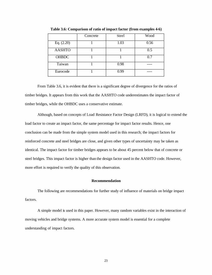
Table 3.6: Comparison of ratio of impact factor (from examples 4-6)

Concrete Steel Wood

Eq. (2.20) 1 1.03 0.56

AASHTO 1 1 0.5

OHBDC 1 1 0.7

Taiwan 1 0.98 ----

Eurocode 1 0.99 ----

From Table 3.6, it is evident that there is a significant degree of divergence for the ratios of

timber bridges. It appears from this work that the AASHTO code underestimates the impact factor of

timber bridges, while the OHBDC uses a conservative estimate.

Although, based on concepts of Load Resistance Factor Design (LRFD), it is logical to extend the

load factor to create an impact factor, the same percentage for impact factor results. Hence, one

conclusion can be made from the simple system model used in this research; the impact factors for

reinforced concrete and steel bridges are close, and given other types of uncertainty may be taken as

identical. The impact factor for timber bridges appears to be about 45 percent below that of concrete or

steel bridges. This impact factor is higher than the design factor used in the AASHTO code. However,

more effort is required to verify the quality of this observation.

Recommendation

The following are recommendations for further study of influence of materials on bridge impact

factors.

A simple model is used in this paper. However, many random variables exist in the interaction of

moving vehicles and bridge systems. A more accurate system model is essential for a complete

understanding of impact factors.

24

A large difference in research is evident between composite and non-composite materials.

Construction methods also influence the material properties. Therefore, it is necessary to investigate the

sensitivity of models to different properties which result from construction of bridges with different

designs.

Constant, single -point, loading is used in this paper, however multi-point loading should be used

to model multi-axle vehicle loading in future studies.

Multi-span bridge systems should be considered in future research.

The interaction of the suspension system of vehicle loading to the roadway roughness is a

complex and important parameter in models of bridge dynamics. This extension is to include the

suspension system of the vehicle loading has been shown to be important in predicting dynamic loading.

The dynamic impact factor is defined based on the ratio of dynamic deflection to static deflection.

The stress rather than the deflection of the bridge is of primary importance. The relationship between the

impact factor and resultant dynamic stress should be considered in future research.

25

REFERENCES

1. LRFD (Load and Resistance Factor Design) Bridge Design Specifications, AASHTO (American

Association of State Highway and Transportation Officials), Washington D. C., 1994.

2. Eui-Seung Hwang and Andrzej S. Nowak, “Dynamic Analysis of Girder Bridges,” 1989, Transportation Research Record 1223, pp 85-92, National Research Council, Washington D. C.

3. B. Bakht and S. G. Pinjarkar, “Dynamic Testing of Highway Bridges- A Review,” 1989, Transportation Research Record 1223, pp 93-100, National Research Council, Washington D. C.

4. A. H. Fuller, A. R. Eitzen, and E. F. Kelly, “Impact on Highway Bridges,” Transactions, ASCE, vol. 95, 1931, pp 1089-1117.

5. R. Cantieni, “Dynamic Load Tests on Highway Bridges in Switzerland : 60 years experience of EMPA,” Report 271, Swiss Federal Laboratories for Materials and Testing Research, Dubendorf, 1983.

6. B. Bakht, “Soil-Steel Structure Response to Live Loads,” Journal of the Geotechnical Engineering Division, ASCE, vol. 107, No. GT6, 1981, pp 779-798.

7. J. R. Billing, “ Dynamic Loading and Testing of Bridges in Ontario,” Proc., International Conference on Short and Medium span Bridges, Toronto, Canada, vol. I, 1982, pp125-139.

8. Ontario Highway Bridge Design Code, Ontario, Ministry of Transportation, Quality and Standards Divisions, Canada, 1983.

9. Paultre, P., U. Challal, and J. Proulx, “Bridge Dynamics and Dynamic Amplification Factors- A Review of Analytical and Experimental Findings,” 1992, Canadian Journal of Civil Engineering, vol. 19, pp 260-278.

10. Ontario Highway Bridge Design Code, Ontario, Ministry of Transportation, Quality and Standards Divisions, Canada, 1991.

11. Highway Bridge Design Code, Ministry of Transportation, Taiwan, 1987.

12. Eurocode, Committee of European Normalization (CEN), 1995.

13. AASHTO Bridge Design Specifications, Washington D. C., 1989.

14. Introduction to Structural Dynamics, John M. Biggs, McGraw-Hill, Inc. 1964.

15. Design of Highway Bridges, Richard M. Barker and Jay A. Puckett, John Willey & Sons, Inc. 1997.