a short introduction to r - personal homepages - vub

A short introduction to R

Luc Hens∗

Vrije Universiteit Brussel & Vesalius College

1 September 2014

Abstract

Aimed at students and teachers in an introductory statistics class orin an economics, business, or other social science class with an empiricalcomponent, this paper introduces the open-source statistical software Rwith the help of simple examples. (Econlit A220, C800)

1 What is R?

R is freely available open-source statistical software comparable to commer-cial (and often expensive) statistical software packages. R runs on Windows,MacOS, and Linux. I have used R for applied statistical work and graphingfunctions in a standard introductory statistics class and in economics classesat the undergraduate and graduate level. The aim of this paper is to give aself-contained introduction to R that demonstrates its capabilities as a teachingand research tool. This paper suffices to get started with R.

To download R, go to the R Project Home page (r-project.org) and follow the“Download” link. Select a mirror site nearby (in Belgium or nearby if you are inBelgium). Select your operating system. For MacOS 10.5 or higher, downloadthe setup program by clicking on the link R-3.1.1.pkg; the version number (3.1.1)may be more recent. For Windows, follow the link to the base distribution anddownload the setup program. Once downloaded, double-click the setup programto install R on your hard disk. If you use a smartphone, a tablet, or a computerwhere you can’t install R (for instance, because the computer is not yours), youcan run R in a web browser on Rweb (http://pbil.univ-lyon1.fr/Rweb/).You can store your R scripts and the results of the computations using freecloud services like Simplenote or Dropbox.

R is not menu-driven but uses command lines (objects, to be exact). Whenyou start R, a console window opens showing a prompt (>) at the bottom. Incommand-line software, the user writes a command after the prompt and presses“enter” to execute the command. Try this: after the prompt, type:

citation()

and press enter. The console will show the bibliographical information neededto cite R in research papers (including homework assignments; you still have

∗I would like to thank my students and Camille Vanderhoeft for comments on earlierversions of this paper.

1

to adapt the bibliographical information to the required citation style). Typedate() and press enter to display the date and time.

First, R is a calculator: to compute 2 + 5 type:

2+5

and press return. The arithmetic operators are +, -, / (division), * (multiplica-tion) and ^ (power: 23 is 2^3). To take the square root of 2 do sqrt(2).

Calculators and computer programs sometimes report numbers using scien-tific notation: 2.345e+04, where e (“exponent”) means “times ten raised tothe power . . . .” For instance, 2.345e+04 means 2.345 times 10 to the power 4:

2.345e+04 = 2.345 × 104 = 2.345 × 10000 = 23450

Similarly, 2.345e–04 means:

2.345e–04 = 2.345 × 10−4 = 2.345 × 1

10000= 0.0002345

R internally uses full precision numbers but typically displays only sevenmeaningful digits on screen. For instance, display the mathematical constantπ = 3.14 . . .:

print(pi)

You can display values with more than seven digits by adding the argumentdigits= the desired number of digits:

print(pi,digits=22)

The assignment operator <- assigns something (a value, a list of values,a formula) to an object. To create an object called shoesize and assign to itthe value 42, do

shoesize <- 42

To display the contents of the object shoesize type

print(shoesize)

(Just printing the object’s name and pressing return displays the object, too;try this).

Lists are defined by the concatenate function c(). To create an object calledmy.grades containing a list of last semester’s grades, do something like:

my.grades <- c(3.0, 3.3, 2.7, 2.3, 3.7)

Display the list by typing print(my.grades) or just my.grades.Lists can contain descriptive phrases or words rather than numbers:

my.favorite.vegetables <- c("broccoli","carrots","red beans")

R is case-sensitive: it makes a difference between upper-case and lower-caseletters. If you defined an object as shoesize (with a lower-case) and give thecommand print(Shoesize), R will respond that it doesn’t know the variableShoesize (with an upper-case).

Comments are useful to annotate R code you’d like to re-use or to documentthe sources of data files. You can insert comments in R code and data files bystarting the comment with a hash (#):

2

# The following line computes 2 times 3:

2*3

You can put a comment after a command in the same line:

2*3 # the preceding code computes 2 times 3

R is well documented. The official documentation is Venables et al. (2006)and there is plenty of additional information geared towards novices on the Rweb site (www.r-project.org , follow the link “Documentation”). If you wantto use R more intensively (for instance, for a masters thesis) I recommend tobuy one of the following books: Adler (2010), Crawley (2002), Crawley (2007),Dalgaard (2002), Fox (2002), or Verzani (2005). All are accessible to novices;I found Adler (2010) the most congenial and Crawley (2007) the most compre-hensive. You can invoke R’s built-in help by typing help.search followed bya description of the topic, enclosed in brackets and quotes. For example, if youwant to find out how to draw a box plot in R, type:

help.search("box plot")

To ask R’s help regarding a specific command—for instance, to know moredetails about how to use the date command—type:

help(date)

The menu bar of R gives access to a built-in text editor. You can usethis text editor to write R code or to create and edit data files. The texteditor also can open, edit, and save plain text files. A plain text file containsonly standard text characters (the characters on your keyboard), no formattinginformation (such as font type or font size), and often has the extension .txt.To open an existing text file, do: File > Open Document . . . . To create a newtext file, do: File > New Document. To save the file, do: File > Save. R willsave the text file with an .R extension.

If you want R to execute a line of code in the text editor, set the cursor tothe line and choose: Edit > Execute. To execute several lines of code, highlightthe code and choose: Edit > Execute.

By saving code in a separate text file, you can adapt and re-use it later.Add comment lines (starting with #) to annotate code in the text file. Teachersmay want to distribute the R code used in the course to their students. For anexample see the file STA101_R_code.R posted on the course web site of STA101.

2 Entering data

In order to be readable by R, data should follow a number of rules:

• Variable names should either contain no blank spaces and commas (year.of.birth)or be enclosed in quotes ("year of birth"). If the variable names areenclosed in quotes, the attach command (see below) will automaticallyreplace all characters that are not allowed (such as blank spaces and com-mas) by periods. For instance, the variable name "year of birth" willbe replaced by year.of.birth.

3

• Numbers should use decimal points (not commas), have no separator forthousands, and have no currency symbol. For example, $1,234,567.89should appear as: 1234567.89 (see below what to do if your spreadsheetdata have decimal commas).

• Values of qualitative data that are character strings (not numbers) cancontain blank spaces or commas but should be enclosed in quotation marks(same left as right): the variable “major” can take the value "International Affairs".

• Non-available values should be coded as NA, not as blanks or as the spread-sheet code #N/A (with a hash). NA should be capitalized: use NA, not na).

Small data sets can be entered in a command line. Suppose in an economythe primary sector accounts for 5 percent, the secondary sector for 35 percent,and the tertiary sector for 60 percent. A quick way to enter the data as lists(the blank spaces—optional—improve readability):

sector <- c("Primary","Secondary","Tertiary")

share <- c( 0.05 , 0.35 , 0.55 )

The operator <- assigns values to the objects (variables) sector and share.You can now use the objects “sector” and “ share” by calling their name. Typethe name of each object and press return to display its contents:

sector

share

It is a good idea to bind the values for the variables together by case (thatis, to make clear that the share 0.05 belongs to the primary sector, the share0.35 belongs to the secondary sector, and the share 0.55 belongs to the tertiarysector). The data.frame command does exactly this:

my.data <- data.frame(sector,share)

Display the data frame “my.data” by typing its name and pressing enter:

my.data

You can now call the variables in the data frame “my.data” by typing thename of the data frame followed by a dollar sign and the name of the variable(name.of.data.frame$name.of.variable):

my.data$sector

my.data$share

I strongly recommend to import large data sets or data sets involving morethan one variable from an external file (which will often be a spreadsheet file)rather than using the method just described. The command to import a dataset from an external file is read.table(). In what follows, I’ll use a data setconsisting of 30 students’ sex, height (cm), weight (kg), and major shown inappendix B. If you are on-line, you can load this data set using:

students <- read.table(

"http://homepages.vub.ac.be/~lmahens/students.csv",

header=TRUE,sep=",")

attach(students)

students # displays the data

names(students) # shows the names of variables

4

A simple way to enter small numeric data sets stored in a spreadsheetfile is to use the scan() command. Assume you collected the values of twostock market indices (DJIA and S&P 500) for five days. Use your spreadsheetprogram to create a new spreadsheet (in LibreOffice.org Calc: File > New >Spreadsheet). Enter the data with variables as columns, elements (cases) asrows:

column A column Brow 1 "DJIA" "SP500"

row 2 10425 1387

row 3 10220 1346

row 4 9862 1333

row 5 10367 1409

row 6 99929 1395

Save the spreadsheet file. Select the DJIA data in cells A2:A6 (don’t includethe header with the variable name) and copy. In the R console, type afterthe prompt: DJIA <- scan() and press enter. After the prompt 1:, paste thecolumn of data. Press enter twice. R has now loaded the DJIA data. Inspectwhether the values were correctly read: typing DJIA and press enter to displaythe data. Repeat for SP500 (column B): copy cells B2:B6, go the R consoleand type SP500 <- scan(), and paste the column of data. Inspect whetherthe values were correctly read: type SP500 and press enter to display the data.Bind the data in a data frame:

stock.market.data <- data.frame(DJIA,SP500)

Although the scan() method is simple, the risk of making mistakes is largeand mistakes are hard to spot. I recommend to use the read.table() commandto import any external data file. To learn more about importing data fromexternal files, read Appendix A. As this topic is rather complicated you maywant to skip the appendix for the time being.

3 Descriptive statistics

The sort() function sorts values from small to large and displays them:

sort(height)

To display just the heights of male students do:

height[sex=="Male"]

The function quantile() computes the five-number summary (minimum, firstquartile, median, third quartile, maximum); summary() computes the five-number summary and the mean:

quantile(height)

summary(height)

To compute descriptive statistics (mean, median, variance, and standard devi-ation) use the following functions:

5

mean(height)

median(height)

var(height)

sd(height)

The variance and standard deviation commands (var and sd) use the formula forsample data (with n− 1 in the denominator). This means that the R commandsd produces SD+ from Freedman, Pisani, & Purves (2007, p. 74), not SD. Tocompute SD for the height do:

number.of.entries <- length(height)

sqrt((number.of.entries-1)/number.of.entries)*sd(height)

To obtain a specific quantile (say, the 90th percentile) use:

quantile(height,.90)

There are different ways to compute quantiles (see help(quantile)), leadingto (usually) slightly different outcomes. To get the 90th percentile as defined inAnderson et al. (2007, p. 69) use:

quantile(height,.90,type=2)

All of the objects above can also be applied to the height of just the male(ot just the female) students, e.g.:

summary(height[sex=="Male"])

To cross-tabulate two variables use table(variable1,variable2). For exam-ple, to cross-tabulate sex and major from the students.csv data set, do:

table(sex,major)

4 Displaying data and distributions

To get a density histogram of the heights use:

hist(height, right=FALSE, freq=FALSE)

The convention in histograms is that class intervals include the left endpoint butnot the right, that is, the 150-to-160 cm interval includes 150 cm and does notinclude 160 cm. This is achieved with the argument right=FALSE. The argu-ment freq=FALSE is needed to get a density histogram: in a density histogram,the vertical scale is a density scale showing the proportion per horizontal unit(crowding) and the relative frequencies are the areas of the bars (Freedman,Pisani, & Purves, 2007, Chapter 3). To plot a frequency histogram where therelative frequencies are the heights of the bars—as in Anderson et al. (2007, p.33)—use the argument freq=TRUE.

To omit the title use the argument main="" (usually one types the title ofa figure in a word processor or layout program). You can control the labels ofplots with the xlab and ylab arguments. The label should be a string delimitedby quotes:

hist(height, right=FALSE, freq=FALSE, xlab = "Height (cm)")

6

R chooses appropriate class intervals, but you can control the number of classes(say, five) with the argument nclass=5 or the class limits between class intervals(breaks) with the argument breaks=c(150,160,170,180,190,200):

hist(height, right=FALSE, xlab = "Height (cm)", freq=FALSE,

breaks=c(150,160,170,180,190,200))

To retrieve the information needed to make a frequency table (class limits,frequencies) use:

hist(height, right=FALSE, freq=FALSE, plot=FALSE)$breaks

hist(height, right=FALSE, freq=FALSE, plot=FALSE)$counts

You can compute the relative and percentage relative frequencies as:

hist(height, right=FALSE, freq=FALSE, plot=FALSE)$counts/length(height)

hist(height, right=FALSE, freq=FALSE, plot=FALSE)$counts/length(height)*100

R often surrounds graphs by a box. Omit the box—as recommended by Tufte(1983, p. 127)—by adding the argument frame.plot=FALSE to the commandto generate the graph.

To obtain a stem-and-leaf display of heights use:

stem(height)

To obtain a box plot of heights use:

boxplot(height,frame.plot=FALSE)

To compare the distributions of two (or more) variables in parallel box plots(only meaningful if all variables are measured on the same scale with the sameunits of measurement) use boxplot(variable1,variable2,...). Let us com-pare the distributions of male and female students’ heights :

boxplot(height[sex=="Male"],height[sex=="Female"])

or, more elegantly:

boxplot(height ~ sex,frame.plot=FALSE)

Pie charts are a poor way to display counts of nominal data; use a bar chartinstead or—usually the best choice—display the frequency table. To generate abar chart or a pie chart of the sector shares do:

barplot(share, names = sector)

pie(share, labels = sector)

5 Scatter plots and the line of best fit

The workhorse command to make plots from data is plot(): depending onthe context, it generates scatter plots, time series diagrams, line diagrams, andmore. By adding arguments you can control the appearance of the plot: labelthe axes, control ticks and tick marks, use colors, add annotations, and muchmore.

To make a scatter plot of heights on the x -axis and weights on the y-axisuse:

7

plot(height,weight)

To control the labels (for instance, to include the units of measurement of thevariables) use the xlab and ylab arguments. The labels should be stringsdelimited by quotes:

plot(height,weight,xlab="Height (cm)",ylab="Weight (kg)",

frame.plot=FALSE)

To find the covariance and the coefficient of correlation use:

cov(height, weight)

cor(height, weight)

If there are missing values, use:

cor(height, weight, use="complete.obs")

To find the line of best fit or regression line between weight (as the dependentvariable) and height (as the independent variable) use:

fitted.model1 <- lm(weight ~ height)

In the lm object, put the dependent (y-axis) variable first, then a tilde (~)meaning “is modelled by,” then the independent (x-axis) variable. lm standsfor linear model; fitted.model1 is the name you assigned to the fitted modeland can be any name. To display the coefficients, their standard deviations,t-statistics and p-values, and the coefficient of determination (R2) use:

summary(fitted.model1)

To display just the coefficients use:

coef(fitted.model1)

To store and display the fitted values (y) use:

weight.fitted <- fitted(fitted.model1)

weight.fitted

To make a scatter plot of heights on the x -axis and weights on the y-axis dis-playing the line of best fit, first make the scatterplot:

plot(height,weight, xlab="Height (cm)",ylab="Weight(kg)",

frame.plot=FALSE)

then add the line of best fit (regression line):

lines(height,weight.fitted)

or:

abline(fitted.model1)

8

6 Pasting a graph in a word processor document

If you want to paste a graph in a word processor document, do the following.In Windows, bring the R window with the graph to the front. Do Edit > Copy.Go to your word processor document and do Edit > Paste. In MacOS, bringthe R window with the graph to the front. Choose Edit > Copy. Start thePreview application and in Preview do File > New From Clipboard. Save asa .png fie. You can now copy and paste the graph from Preview into a wordprocessor document.

To save a graph, bring the window with the graph to the front and choose inthe R menu File > Save as . . . . In Windows, save in the .png format. In MacOS,save as .pdf—that’s the only option, but you can open the .pdf in Preview andsave in .png.

7 Probability distributions

To randomly draw five numbers between 1 and 50 with and without replacementtype:

sample(1:50,5,replace=TRUE)

sample(1:50,5,replace=FALSE)

The binomial formula (Freedman, Pisani & Purves, 2007, p. 259) is com-puted using dbinom(k,n,p). More concretely, consider a binomial experimentwith 10 trials and a probability that the event of interest occurs (“success”) of0.4. To find the probability of 6 successes do:

dbinom(6,10,0.4)

To get a list all probabilities (of 0, 1, 2, ..., 10 successes) do:

dbinom(0:10,10,0.4)

To plot the normal curve do:

x <- seq(-4,+4,length=400)

y <- dnorm(x)

plot(x,y,ylab="f(x)",type="l",frame.plot=FALSE)

The cumulative normal distribution pnorm computes the area in the left tail ofthe normal curve with a mean of 0 and a standard deviation of 1 (the standardnormal curve). To find the area under the normal curve to the left of −2 do:

pnorm(-2)

To find the area under the normal curve to the right of 2 do:

pnorm(2, lower.tail=FALSE)

To find an area under the normal curve between some lower boundary (say, −1)and some upper boundary (say, +2) do:

pnorm(2) - pnorm(-1)

To compute this area and plot the normal curve with the shaded area do:

9

xlo <- -1 # the lower boundary

xup <- 2 # the upper boundary

# you don’t have to change anything in the code below:

pnorm(xup) - pnorm(xlo)

cord.x <- c(xlo,seq(xlo,xup,0.01),xup)

cord.y <- c(0,dnorm(seq(xlo,xup,0.01)),0)

curve(dnorm(x),xlim=c(-4,+4), ylab="f(x)",frame.plot=FALSE)

polygon(cord.x,cord.y,col="grey",lty="blank")

Verify the empirical rule by computing:

pnorm(+1) - pnorm(-1)



The procedures to find areas under the Student t-distribution curve aresimilar. The cumulative t-distribution is pt, and the arguments of the functionare the upper boundary and the degrees of freedom. For example, to find thearea to the left of +2 under a t-curve with 18 degrees of freedom do:

pt(+2, df = 18)

To find the area between -2 and +2 under a t-curve with 18 degrees of freedomdo:

pt(+2, df = 18) - pt(-2, df = 18)

To compute the area and plot the t density curve with the shaded area do:

tdf <- 18

tlo <- -2

tup <- +2

# you don’t have to change anything in the code below:

pt(tup, df = tdf) - pt(tlo, df = tdf)

cord.x <- c(tlo,seq(tlo,tup,0.01),tup)

cord.y <- c(0,dt(seq(tlo,tup,0.01),df=tdf),0)

curve(dt(x,df=tdf),xlim=c(-3,+3),xlab="t", ylab="f(t)",

frame.plot=FALSE)

polygon(cord.x,cord.y,col="grey",lty="blank")

To find quantiles of a variable that follows the normal distribution, use theqnorm function. To find the 25th percentile of a variable that follows the normaldistribution with a mean of 20 and a standard deviation of 5 do:

qnorm(.25, mean = 20, sd = 5)

To find the 25th percentile of the t-distribution with 18 degrees of freedom do:

qt(.25, df = 18)

10

8 Confidence intervals and hypothesis tests

Freedman, Pisani, & Purves (2007) use z-tests rather than t-tests most of thetime. That’s OK if the sample is sufficiently large: in that case the test statisticsand P -values for the z-test and t-test will be very similar. R has no z-testprocedure—use a t-test instead. Here’s how the t.test procedure works.

Assuming that the variable weight is normally distributed and the sampleis a simple random sample, the 95 percent confidence interval for the populationmean is obtained by:

t.test(weight, conf.level = .95)$conf.int

Suppose you would like to test hypotheses concerning the average weight ofthe population. Assuming that weights are normally distributed and the sampleis a simple random sample, a t-test is the appropriate method. To test the nullhypothesis that the population average (usually denoted by µ, the Greek letter“mu”) is 64 kg against the two-sided alternative that the population averagediffers from 64 kg (in either way) do:

t.test(weight, mu = 64)

To test the null hypothesis that the population average is 64 kg against theone-sided alternative that the population average is less than 64 kg do:

t.test(weight, alternative = "less", mu = 64)

To test the null hypothesis that the population average is 64 kg against theone-sided alternative that the population average is greater than 64 kg do:

t.test(weight, alternative = "greater", mu = 64)

To find a confidence interval or do a hypothesis test on a proportion or apercentage use binom.test. Suppose that you took a simple random sampleof 1,600 persons, of which 917 people are Democrats (Freedman, Pisani, &Purves, 2007, example 2 p. 382). To get the 95 percent confidence interval forthe proportion use:

binom.test(917, 1600, conf.level = .95)$conf.int

To get the 95 percent confidence interval for the percentage multiply by 100%:

100*binom.test(917, 1600, conf.level = .95)$conf.int

To test the null hypothesis that the percentage of Democrats in the populationis 55% against the one-sided alternative that the percentage is greater than 55%,do:

binom.test(917, 1600, 0.55, alternative = "greater")

9 Time series

If you work with annual time series and don’t need specific time series operationssuch as lagging a variable or make time series diagrams, the commands abovewill get you a long way. Suppose you have an annual time series of a price indexfor a country starting in 1993. The numbers can be entered as follows:

11

year <- c(1993,1994,1995,1996,1997,1998,1999)

price <- c(90.1,92.3,95.3,96.1,97.2,99.0,100.0)

You can now make a scatter plot, compute a time trend and so on. However,it’s often useful and sometimes necessary to create a time-series object. Thecommand ts() creates a time series (usually called price.ts or so) from anexisting variable price as follows:

price.ts <- ts(price,start=c(1993,1))

price.ts # displays the time series

Suppose your data have four observations per year, one for each quarter. Here’sa time series of quarterly real GDP starting in the first quarter of 1991 (expressedas an index, 2000 = 100):

gdp <- c(86.0,85.3,84.9,86.1,87.7,87.0,87.0,87.0,86.0,86.1,86.8)

Create a time series object as follows:

gdp.ts <- ts(gdp,start=c(1991,1),frequency=4)

gdp.ts # displays the time series

frequency = 4 means that there are four observations (quarters) per unit oftime (year). To plot the time series do:

plot(gdp.ts,ylab="Real GDP (index, 2000 = 100)",frame.plot=FALSE)

To compute and plot a linear time trend do:

fitted.time.trend <- lm(gdp.ts ~ time(gdp.ts))

abline(fitted.time.trend, lty="dashed")

lty stands for “line type” (in this case, a dashed line). To display the coefficientsand other statistics of the time trend use:

summary(fitted.time.trend)

To lag the time series by one period (in this case, one quarter) do:

lag(gdp.ts, k = -1)

To obtain the quarter-on-quarter growth rate of GDP do:

(gdp.ts-lag(gdp.ts,k=-1))/lag(gdp.ts,k=-1)

To obtain the year-on-year growth rate of quarterly GDP do:

(gdp.ts-lag(gdp.ts,k=-4))/lag(gdp.ts,k=-4)

Multiply by 100 to obtain percentage growth rates.R can also work with multivariate time series. The relationship between

unemployment and inflation is known as the Phillips curve. The following dataare annual time series of the unemployment rate and the inflation rate for acountry starting in 1993:

unemployment <- c(10.6,9.5,8.2,8.2,8.3,7.7,6.9,6.3,6.8,6.4,6.1)

inflation <- c( 1.4,0.8,1.5,2.2,1.5,0.2,0.5,4.3,3.8,2.9,2.8)

12

Create the time series variables:

inflation.ts <- ts(inflation ,start=c(1993,1),frequency=1)

unemployment.ts <- ts(unemployment,start=c(1993,1),frequency=1)

Plotting both series in a single diagram makes sense because they are measuredon the same scale and use the same units (percent). To plot both series overtime in a single time series diagram do:

ts.plot(inflation.ts,unemployment.ts,lty=c(1:2),frame.plot=FALSE)

legend("topright",legend=c("Inflation","Unemployment"),lty=c(1:2))

The argument lty=c(1:2) uses two different line types for the two series; touse different colors do:

ts.plot(inflation.ts,unemployment.ts, col=c(1:2),frame.plot=FALSE)

legend("topright",legend=c("Inflation","Unemployment"),lty=1,col=c(1:2))

You can explore the relationship between two time series by making a scatterplot and drawing the line of best fit. The command

plot(unemployment.ts,inflation.ts,frame.plot=FALSE)

will generate a scatter plot with points labeled by time and connected by linesshowing the time path. To obtain a plain vanilla scatter plot (with pointsindicating the observations, no time labels, no time path), use:

plot(unemployment.ts,inflation.ts,frame.plot=FALSE,xy.labels=FALSE)

(I omitted the xlab and ylab arguments for clarity.) To add the line of best fitand compute the coefficient of correlation, do:

Phillips.curve.fitted <- lm(inflation.ts ~ unemployment.ts)

abline(Phillips.curve.fitted)

cor(unemployment.ts,inflation.ts, use="pairwise.complete.obs")

(The following section is quite technical. You may want to skip it.)Working with the linear model object (lm) is tricky with time series objects,especially when there are missing values (NA) or time lags (see the R Helpentry on lm). Suppose you would like to estimate the relationship betweenunemployment and the change in the inflation rate (a simplified form of theexpectations-augmented Phillips curve). First, create and display a new timeseries of the change in the inflation rate:

change.in.inflation.ts <- inflation.ts - lag(inflation.ts, k = -1)

change.in.inflation.ts

The time series change.in.inflation starts one period later than inflation.If you try to estimate the linear relationship between unemployment and thechange in the inflation rate, R returns an error message because the two seriesare not of the same length. To make both series of the same length, use thecommand ts.union, which binds the two time series by padding the shorterseries with NAs to the total time coverage. The resulting new data frame(data2 in the example below) will have the same start and end period for allvariables:

13

data.Phillips <- ts.union(change.in.inflation.ts,unemployment.ts,dframe=TRUE)

data.Phillips

Attaching the new data frame won’t work because the variable names are alreadyin use, but you can call the new variables by:

data.Phillips$change.in.inflation.ts

data.Phillips$unemployment.ts

Here’s how to make the scatter plot, add the line of best fit, and computethe coefficient of correlation (again, I omitted the frame.plot=FALSE,xlab andylab arguments for clarity):

augmented.Phillips.curve.fitted

<- lm(data.Phillips$change.in.inflation.ts ~ data.Phillips$unemployment.ts)

summary(augmented.Phillips.curve.fitted)

cor(data.Phillips$unemployment.ts,data.Phillips$change.in.inflation.ts,

use="pairwise.complete.obs")

plot(data.Phillips$unemployment.ts,data.Phillips$change.in.inflation.ts,

xy.labels=FALSE)

abline(augmented.Phillips.curve.fitted)

To learn more about using R for advanced time series work, consult Pfaff (2006)or Shumway & Stoffer (2006).

10 Plotting functions

R is an excellent tool to plot mathematical functions. Consider the followingsupply and demand schedules:

Qs = 10 + 40P

Qd = 100 − 20P

Solve both equations for the y-axis variable (P ):

P = −10

40+

1

40Qs

P =100

20− 1

20Qd

Use seq to define the desired range of Q (here, 0 to 150 is fine, but the appro-priate range depends on the problem at hand; you may have to experiment abit):

Q <- seq(0,150)

Then define the supply and demand functions:

Ps <- -(10/40) + (1/40)*Q

Pd <- (100/20) - (1/20)*Q

Use plot to draw the supply schedule:

plot(Q,Ps,xlab="Quantity (kg)",

ylab="Price (euros per kg)",type="l")

14

Use lines to add the demand schedule to the plot you just created:

lines(Q,Pd)

Another method uses the curve(expression,from,to,...) command:

curve(-(10/40)+(1/40)*x,0,150,

xlab="Quantity (kg)", ylab="Price (euros per kg)")

curve((100/20)-(1/20)*x,add=TRUE) # adds the demand curve

To add text (such as the labels “Supply” and “Demand”) first locate the coor-dinates of the places where you want to position the text. Enter the instructionlocator(2), press enter, and then click with the left mouse button on the twopositions in the graph window. The console returns the coordinates. Then usetext:

text(130,2.6,"Supply")

text(120,0,"Demand")

The instruction locator(1) will also give the (approximate) location of theintersection between the supply and demand curve. To get the exact equilibrium(Q = 70, P = 1.5) you have to solve the system of equations. The R command tosolve systems of equations (solve) requires you to write the system of equationsin matrix form and is beyond the scope of this paper. To plot the equlibriumpoint (70, 1.5) and dashed lines showing the coordinates do:

points(70,1.5)

segments(70, 0 , 70, 1.5, lty="dashed", col="grey") # vertical

segments( 0, 1.5, 70, 1.5, lty="dashed", col="grey") # horizontal

A simple way to add a straight line to an existing plot uses the abline

function. Read abline as a-b line: a is the intercept and b is the slope orgradient of the line with equation y = a + bx. For instance, suppose that thedemand schedule shifts to:

P =120

20− 1

20Qd

To add the new demand schedule as a dashed line do:

abline(a = 120/20, b = -1/20, lty = "dashed")

lty stands for “line type”; if you omit the lty argument, abline and lines

plot a solid line. Alternatively, you can use:

curve(120/20-(1/20)*x, lty = "dashed", add=TRUE)

11 Troubleshooting R

The first things you should do when you have a problem is to check this doc-ument and use R’s built-in help function (for example, if you have a problemwith the cor command, type help(cor)). Here are some frequent problems andpossible solutions.

Problem 1. The read.table command doesn’t work. I get the error message:

15

Error in file(file, "r") : unable to open connection

In addition: Warning message:

cannot open file ’.....’, reason ’No such file or directory’

Solution: You probably made an error in the location of the data file. Care-fully check the location of the data file and compare with the location in theread.table command. Make sure you used forward leaning slashes (/), notbackslashes, and the proper identical quotes ("...", not “...”). Make sure thatthe data file is a plain text file with the .cvs or .txt extension.

Problem 2. The read.table command doesn’t work. I get the error message:

Error in read.table("...", header = TRUE, :

more columns than column names

or:

Error in scan(file, ..., na.strings, :

line 1 did not have 10 elements

Solution: Open the file in a text editor (Notepad, TextEdit). Check that thedata file has the required format: the first line contains variable names separatedby blank spaces or commas, subsequent lines contain the data values separatedby blank spaces commas. There should be as many data values per line as thereare variable names in line one. In a comma-separated file, verify that there areno redundant commas; remove redundant commas.

Problem 3. I loaded my data set using read.table. When I try to manip-ulate one of the variables (print, plot, compute descriptive statistics, ...) I getthe error message:

Error: object "..." not found

Solution: Type ls() (“list”) and press enter to see a list of the data sets inyour workspace (including the variable names generated using the attach(...)command). If the variable names don’t appear, you probably forgot to attachthe database. If the problem still occurs after you attached the database, checkwhether you included the separator (sep) argument in the read.table com-mand.

Problem 4. I typed a command and pressed enter. Nothing happened, ex-cept that the R console returns a + prompt instead of the usual < prompt.Solution: The + prompt indicates that R expects additional input. Proba-bly your previous command was incomplete; you may have forgotten a closingbracket or other input. Type the missing part of the command after the +

prompt and press enter.

Problem 5. The cor command doesn’t work. I get the error message:

Error in cor(variable1,variable2) :

missing observations in cov/cor

Solution: Your variable1 or variable2 contains missing observations (coded asNA). In that case, you have to specify what cor should do with missing obser-vations:

16

cor(variable1,variable2, use = "complete.obs")

Check help(cor) for details.

Problem 6. I tried to plot a line of best fit in the scatter plot. I don’t getan error message, but the line of best fit doesn’t appear in the scatter plot.Solution: You probably confused the y- and x-axis variables in the lm(y ~ x)

command: in the lm(y ~ x) command the y-axis variable should come first,while in the plot(x,y) command the x-axis variable should come first. y ~ x

means “y modelled by x.”

A Appendix: Importing data from an externalfile

This is an advanced topic. You can skip it if you just want to get a quickintroduction to R, but you have to read it if you want to use R for more seriouswork.

A.1 The read.table() command

It’s a good idea to store your data on a external file and import them to R theread.table() command. For beginners, importing data from an external fileis the most challenging part of getting started with R (or any other statisticalsoftware). R is flexible and can import data from files in many different ways;I’ll explain just one method (importing from a comma-separated values file).

I recommend to store all your R data in the same location. Create a newdirectory R Data in the Documents directory (MacOS) or My Documents di-rectory (Windows). Download the data file students.csv from my Statistics 101home page (Hens, 2007):

http://homepages.vub.ac.be/~lmahens/students.csv

Store students.csv in the R Data directory on your hard disk. It is importantthat your operating system shows the complete data file names including theextensions such as .txt and .csv. To view the extension of a file do the following:

– MacOS: select the relevant file(s) in the Finder and choose File > GetInfo; then click Name & Extension and deselect the ”Hide extension”checkbox(es).

– Windows: Open the R Data directory in My Computer. In the menubar of the R Data directory, choose Tools > Folder options . . .> View.Uncheck the box “Hide extensions (. . . )”. This will display the extensionsof all the files in the R Data directory.

The data should be in a plain text file (see above) with a specific format:

– Variables should be in columns, elements (cases) in rows.

– The first line should contain the variable names. The subsequent linescontain the data values. It’s possible to include comment lines to doc-ument the source and units of measurement of the data; comment linesshould start with a hash (#).

17

– Variable names and values should be separated by commas. That’s whysuch a text file is called a comma-separated values file and gets theextension .csv rather than the extension .txt. Many databases offer theoption to export data to a csv formatted file. Section 2.3 explains how toexport spreadsheet files to csv files.

Open the file students.csv with a text editor (like TextEdit in MacOS orNotePad in Windows) to see an example of a data file in plain text format.This data set shows the sex, height (in cm), weight (in kg), and major for 30students. It is a file in comma-separated values (csv) text format. I verticallyaligned the columns to improve readability, but this is not required.

"sex" ,"height","weight","major"

"Female", 172 , 63 ,"Business"

"Female", 170 , 70 ,"International Affairs"

"Female", 170 , 52 ,"Other"

"Female", 171 , 52 ,"Communications"

"Male" , 186 , 90 ,"Business"


"Male" , 170 , 66 ,"Communications"


"Male" , 175 , 75 ,"International Affairs"






















Each column represents a variable, and the first row contains the variablenames. The file contains sex, height (in centimeters), weight (in kilograms),major, and year of birth for a group of thirty students. The numbers are notincluded in quotes, the words and descriptive phrases are. Close students.csvbefore proceeding. (If you don’t have students.csv but an electronic versionof this document, copy and paste the data into a text document (in Windowsuse Notepad or Wordpad, in MacOS use TextEdit). Save the document asstudents.csv.)

18

Now we’ll tell R what the working directory is, that is, where to lookfor data. You can set the working directory with the R setwd command. Thecommand will look like this in Mac OS:

setwd("/Users/myMacBook/Documents/R Data")

and like this in Windows:

setwd("C:/Documents and Settings/User/My documents/R Data")

The text in quotation marks is the path to the working directory. To find findthe path to the working directory in Windows, open My Computer and selectany file in the R Data directory. Right-click the file and select Properties. Selectand copy the file location, which will look someting like:C:\Documents and Settings\User\My documents\R Data.

Caution: Windows uses backslashes (\) in the path, but in the setwd() com-mand you should use forward-leaning slashes (/). To find the path to the work-ing directory in Mac OS, select any file in the R Data directory and choose File> Get Info. The “where” item gives the path to the file.

You can also set the working directory via the menu:

– Mac OS: R > Preferences > Initial working directory. Click the “change”button and select the R Data directory you created. In Mac OS R re-members the working directory next time you start R, so you only haveto do this once.

– Windows (method 1): File > Change dir . . . . A dialog window opens.Browse to the R Data directory you created and click OK. In Windows Rdoesn’t remember the new working directory, so you’ll have to redo thisthe next time you start R.

In the R console check the working directory with the command getwd().Now we’re ready to read the comma-separated data table from students.csvstored in the working directory:

students <- read.table("students.csv",header=TRUE, sep=",")

The first part of the command (students <-) assigns the result of the read.tablecommand to an object called students (it can be any valid object name andshould not contain blank spaces). The students.csv argument gives the filename including the extension and enclosed in quotes. The argument header=TRUEindicates that the file contains the names of the variables as its first line (header).The argument sep="," indicates that values on each line of the file are sep-arated by a comma. To display the contents of the students object justtype students. You can now call the variables stored in the object students

as students$sex,students$height, students$weight, and students$major.Try this by typing students$height and pressing enter. It is more convenientto call the variables simply as sex, height, weight, and major. To do this wecreate a “data frame” with the attach() function:

attach(students) # creates a data frame "students"

Now type height and press enter. The console will display the values of thevariable “height.”

19

A.2 Converting a spreadsheet file to a csv file

If the data are in a spreadsheet file (using a format such as .xls, .ods, or .num-bers), first convert the spreadsheet file to a comma-separated values file.Here’s how to do this in LibreOffice.org Calc.1

First, verify whether the spreadsheet program uses decimal points: open anew spreadsheet, type in in cell A1: =pi() (the function to display the mathe-matical constant π = 3.1415927 . . .) and press enter. If the cell displays some-thing like 3.14 (possibly with more decimals) your spreadsheet program usesdecimal points. If the cell displays something like 3,14 (possibly with moredecimals) your spreadsheet program uses decimal commas and the procedure isslightly different (as explained below).

Second, open the data spreadsheet (in the example: students2.ods or stu-dents2.xls) in LibreOffice.org Calc (LibreOffice.org Calc opens Microsoft Excelspreadsheet files). Verify that the variables are in columns and the elements(cases) in rows. In the menu, select File > Save as . . . . A dialog window “Se-lect File Type” appears. Select Text CSV and leave the Hide Extension boxunchecked. The file name in dialog window will automatically get the .csv ex-tension. Select the R Data directory as the location of the .csv file. Then selectSave and click Yes to save as Text CSV. A new dialog window “Export of textfiles” appears. Leave the Character set at its default value. If your data havedecimal points select as Field delimiter a comma (,). If your data have deci-mal commas select as Field delimiter a semicolon (;). Leave the text delimiterat its default value ("). Leave the “Save cell content as shown” box checkedand the “Fixed column width” box unchecked. Note that it’s OK to save withthe .csv extension even if you used semicolons rather than commas to separatedata values. We’ll tell R in the read.table command whether the data fileuses commas or semicolons to separate values.

Open the text file (students2.cvs) in your text editor and clean it up ifnecessary: sometimes the spreadsheet may have had empty but active cells,which will show up in the csv file as redundant value separators (commas orsemicolons) at the end of a line or at the end of the document, or as blanklines at the end of the document—remove them and save the file. You can nowimport the table in R as explained in the previous section. If your data file usesdecimal points and has commas as separators the read.table() commandlooks like:

students2 <- read.table("students2.csv",header=TRUE,sep=",")

If your data file uses decimal commas and uses semicolons to separate val-ues, the read.table command should have as arguments sep=";" (values areseparated by semicolons) and dec="," (numbers have decimal commas):

students2 <- read.table("students2.csv",header=TRUE,sep=";",dec=",")

Type students2$height and press enter to display the heights.

1I recommend LibreOffice.org Calc because it gives the user more control over how thespreadsheet is exported to a csv file. LibreOffice.org Calc opens Microsoft Excel spreadsheetfiles (.xls) and allows to save them as csv files. In Microsoft Excel the instructions to savea spreadsheet file to a csv file start with: File > Save as . . . ; in iWork Pages with: File >Export. Consult the manuals or help functions of Microsoft Excel or iWork Pages for detailson exporting to csv files.

20

A.3 Exporting data to a text file

Assume that you would like to sort the students by height and export the resultto a file. First create a new data frame with the students sorted by height:

students.ordered <- students[order(height),]

(the comma before the closing bracket end is no typo; it should be there.)Then write the new data file to an external file (newdata.txt) in your workingdirectory:

write.table(students.ordered, file="newdata.txt",sep=",")

A.4 The swirl package

The swirl package is an R package that “teaches you R programming and datascience interactively, at your own pace, and right in the R console.” It coversthe same ground as this document, and more. For information on how to installand run swirl, see http://swirlstats.com.

A.5 Built-in data sets and data packages

R comes with number of built-in data sets. To get a list of the the built-indata sets do:

data()

To get a description of one of the data sets (say, ChickWeight) do:

help(ChickWeight)

To display the variable “weight” from the ChickWeight data set do

ChickWeight$weight

More data sets are available as packages. The Penn World Table (“a databasewith information on relative levels of income, output, inputs and productiv-ity, covering 167 countries between 1950 and 2011”—Feenstra et al. (2013)) isavailable as the R package pwt. To install pwt make sure that you are online.Type:

install.packages("pwt8")

Installing a package can take a couple of minutes. You only have to do this onceon the same computer: the command downloads and stores the Penn WorldTable on your hard disk. When the package pwt is installed, call it from thelibrary as follows:

library(pwt8)

You have to repeat library(pwt8) whenever you start a new R session andwant to use the Penn World Table. Open the help file on pwt:

help.start()

21

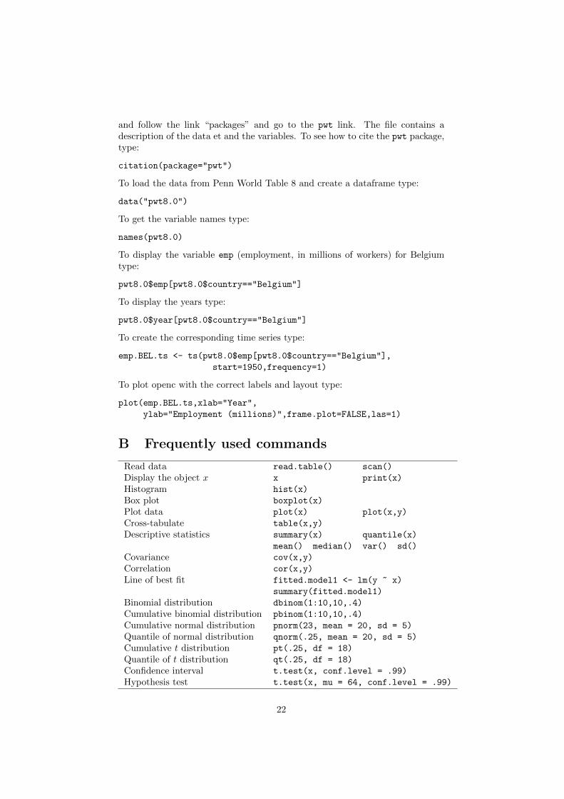
and follow the link “packages” and go to the pwt link. The file contains adescription of the data et and the variables. To see how to cite the pwt package,type:

citation(package="pwt")

To load the data from Penn World Table 8 and create a dataframe type:

data("pwt8.0")

To get the variable names type:

names(pwt8.0)

To display the variable emp (employment, in millions of workers) for Belgiumtype:

pwt8.0$emp[pwt8.0$country=="Belgium"]

To display the years type:

pwt8.0$year[pwt8.0$country=="Belgium"]

To create the corresponding time series type:

emp.BEL.ts <- ts(pwt8.0$emp[pwt8.0$country=="Belgium"],

start=1950,frequency=1)

To plot openc with the correct labels and layout type:

plot(emp.BEL.ts,xlab="Year",

ylab="Employment (millions)",frame.plot=FALSE,las=1)

B Frequently used commands

Read data read.table() scan()

Display the object x x print(x)

Histogram hist(x)

Box plot boxplot(x)

Plot data plot(x) plot(x,y)

Cross-tabulate table(x,y)

Descriptive statistics summary(x) quantile(x)

mean() median() var() sd()

Covariance cov(x,y)

Correlation cor(x,y)

Line of best fit fitted.model1 <- lm(y ~ x)

summary(fitted.model1)

Binomial distribution dbinom(1:10,10,.4)

Cumulative binomial distribution pbinom(1:10,10,.4)

Cumulative normal distribution pnorm(23, mean = 20, sd = 5)

Quantile of normal distribution qnorm(.25, mean = 20, sd = 5)

Cumulative t distribution pt(.25, df = 18)

Quantile of t distribution qt(.25, df = 18)

Confidence interval t.test(x, conf.level = .99)

Hypothesis test t.test(x, mu = 64, conf.level = .99)

22

References

Adler, J. (2010). R in a nutshell. O’Reilly, Sebastopol, CA.

Crawley, M. (2002). Statistics: An Introduction Using R. John Wiley and Sons,London.

Crawley, M. (2007). The R Book. John Wiley and Sons, Chichester (UK).

Dalgaard, P. (2002). Introductory Statistics with R. Springer, Berlin.

Feenstra, R. C., Inklaar, R., and Timmer, M. P. (2013). The Next Generationof the Penn World Table. Available for download at www.ggdc.net/pwt.

Fox, J. (2002). An R and S-Plus Companion to Applied Regression. Sage,London.

Venables, W. N., Smith, D. M., and R Development Core Team (2006). AnIntroduction to R. R Foundation for Statistical Computing, Vienna (Austria).

Verzani, J. (2005). Using R for introductory statistics. Chapman and Hall/CRC,Boca Raton (FL).

23