a short course on mean field spin glasses

A short course on mean field spin glasses

Anton Bovier1 and Irina Kurkova2

1 Weierstrass Institut fur Angewandte Analysis und Stochastik, Mohrenstrasse 39,10117 Berlin, Germany [email protected]

2 Laboratoire de Probabilites et Modeles Aleatoires, Universite Paris 6, 4, placeJussieu, B.C. 188, 75252 Paris, Cedex 5, France [email protected]

1 Preparation: The Curie-Weiss model

The main topic of this lecture series are diordered mean field spin systems.This first section will, however, be devoted to ordered spin systems, and moreprecisely essentially to the Curie-Weiss model. This will be indispensableto appreciate later the much more complicated Sherrington-Kirkpatrick spinglass.

1.1 Spin systems.

In his Ph.D. thesis in 1924, Ernst Ising [18, 19] attempted to solve a model,proposed by his advisor Lenz, intended to describe the statistical mechanics ofan interacting system of magnetic moments. The setup of the model proceedsagain from a lattice, Zd, and a finite subset, Λ ⊂ Zd. The lattice is supposedto represent the positions of the atoms in a regular crystal. Each atom isendowed with a magnetic moment that is quantized and can take only thetwo values +1 and −1, called the spin of the atom. This spin variable at sitex ∈ Λ is denoted by σx. The spins are supposed to interact via an interactionpotential φ(x, y); in addition, a magnetic field h is present. The energy of aspin configuration is then

HΛ(σ) ≡ −∑

x 6=y∈Λ

φ(x, y)σxσy − h∑x∈Λ

σx (1)

The spin system with Hamiltonian (1) with the particular choice

φ(x, y) =

{J, if |x− y| = 10, otherwise

(2)

is known as the Ising spin system or Ising model. This model has played acrucial role in the history of statistical mechanics.

2 Anton Bovier and Irina Kurkova

The essential game in statistical mechanics is to define, once a Hamiltonianis given, a probability measure, called the Gibbs measure , on the space of spin-configuration. This entails some interesting subtleties related to the fact thatwe would really do this in infinite volume, but I will not enter into these here.For finite volumes, Λ, we can easily define this probability as

µβ,h,Λ(σ) ≡ exp (−βHΛ(σ))Zβ,h,Λ

, (3)

where Zβ,h.Λ is a normalizing factor called the partition function,

Zβ,h,Λ ≡∑σ∈SΛ

exp (−βHΛ(σ)) . (4)

An interesting fact of statistical mechanics is that the behavior of the partitionfunction as a function of the parameters β and h contains an enormous amountof information.

We will callFβ,h,Λ ≡ −

1β

lnZβ,h,Λ (5)

the free energy of the spin system.The importance of the Ising model for modern statistical physics can

hardly be overestimated. With certain extensions, some of which we will dis-cuss here, it has become a paradigmatic model for systems of large numbersof interacting individual components, and the applications gained from theinsight into this model stretch far beyond the original intentions of Lenz andIsing.

1.2 Subadditivity and the existence of the free energy

The main concern of statistical mechanics is to describe systems in the limitwhen its size tends to infinity. Hence one of the first questions one asks, iswhether quantities defined for finite Λ have limits as Λ ↑ Zd. The free energy(5) is defined in such a way that one can expect this limit to exists. Sincethese questions will recur, it will be useful to see how such a result can beproven.

It will be useful to note that we can express the Hamiltonian in the equiv-alent form

HΛ(σ) =∑x,y∈Λ

φ(x, y) (σx − σy)2 − h∑x∈Λ

σx (6)

which differs from HΛ only by a constant. Now let Λ = Λ1 ∪Λ2, where Λi aredisjoint volumes. Clearly we have that

Zβ,Λ =∑

σx,x∈Λ1

∑τy,y∈Λ2

exp (−β [HΛ1(σ) +HΛ2(τ)])

× exp

−β ∑x∈Λ1

∑y∈Λ2

φ(x, y)(σx − τy)2

(7)

Mean field spin glasses 3

If φ(x, y) ≥ 0, this implies that

Zβ,Λ ≤ Zβ,Λ1Zβ,Λ2 (8)

and therefore−Fβ,Λ ≤ (−Fβ,Λ1) + (−Fβ,Λ2) (9)

The property (8) is called subadditivity of the sequence (−Fβ,Λ). The impor-tance of subadditivity is that it implies convergence, through an elementaryanalytic fact:

Lemma 1. Let an be a real-valued sequence that satisfies, for any n,m ∈ N,

an+m ≤ an + am (10)

Then, limn↑∞ n−1an exists. If, moreover, n−1an is uniformly bounded frombelow, then the limit is finite.

By successive iteration, the lemma has an immediate extension to arrays:

Lemma 2. Let an1,n2,...,nd , ni ∈ N be a real-valued array that satisfies, forany ni,mi ∈ N,

an1+m1,...,nd+md ≤ an1,...,nd + am1,...md (11)

Then, limn↑∞(n1n2 . . . , nd)−1an1,...,nd exists.If an(n1n2 . . . , nd)−1an1,...,nd ≥ b > −∞, then the limit is finite.

Lemma 2 can be used straightforwardly to prove convergence of the freeenergy over rectangular boxes:

Proposition 1. If the Gibbs free energy Fβ,Λ of a model satisfies the subaddi-tivity property (9), and if supσHΛ(σ)/|Λ| ≥ C > −∞, then, for any sequenceΛn of rectangles

limn↑∞|Λn|−1Fβ,Λn = fβ (12)

exists and is finite.

Obviously this proposition gives the existence of the free energy for Ising’smodel, but the range of applications of Proposition 1 is far wider, and vir-tually covers all lattice spin systems with bounded and absolutely summableinteractions. To see this, one needs to realize that strict subadditivity is notreally needed, as error terms arising, e.g., from boundary conditions can easilybe controlled. Further details can be found in Simon’s book [28].


1.3 The Curie–Weiss model

Although the Ising model can be solved exactly in dimensions one (easy) andtwo (hard), exact solutions in statistical mechanics are rare. To get a quickinsight into specific systems, one often introduces exactly solvable mean fieldmodels . It will be very instructive to study the simplest of these models, theCurie–Weiss model in some detail. All we need to do to go from the Ising modelto the Curie-Weiss model is to replace the nearest neighbor pair interaction ofthe Ising model by another extreme choice, namely the assumption that eachspin variable interacts with each other spin variable at any site of the latticewith exactly the same strength. Since then the actual structure of the latticebecomes irrelevant, and we simply take Λ = {1, . . . , N}. The strength of theinteraction should be chosen of order 1/N , to avoid the possibility that theHamiltonian takes on values larger than O(N). Thus, the Hamiltonian of theCurie–Weiss model is

HN (σ) = − 1N

∑1≤i,j≤N

σiσj − hN∑i=1

σi (13)

At this moment it is time to discuss the notion of macroscopic variables insome more detail. So far we have seen the magnetization, m, as a thermo-dynamic variable. It will be reasonable to define another magnetization as afunction on the configuration space: we will call

mN (σ) ≡ N−1N∑i=1

σi (14)

the empirical magnetization. Here we divided by N to have a specific mag-netization. A function of this type is called a macroscopic function, becauseit depends on all spin variables, and depends on each one of them very little(we will make these notions more rigorous in the next section).

Note that the particular structure of the Curie–Weiss model entails thatthe Hamiltonian can be written as a function of this single macroscopic func-tion:

HN (σ) = −N2

[mN (σ)]2 − hNmN (σ) ≡ NΨh(mN (σ)) (15)

This can be considered as a defining feature of mean field models.Let us now try to compute the free energy of this model. Because of the

the interaction term, this problem looks complicated at first. To overcome thisdifficulty, we do what would appear unusual from our past experience: we gofrom the ensemble of fixed magnetic field to that of fixed magnetization. Thatis, we write

Zβ,h,N =∑

m∈MN

eNβ(m2

2 +mh)zm,N (16)

where MN is the set of possible values of the magnetization, i.e.,


MN ≡ {m ∈ R : ∃σ ∈ {−1, 1}N : mN (σ) = m} (17)= {−1,−1 + 2/N, . . . , 1− 2/N, 1}

andzm,N ≡

∑σ∈{−1,1}N

1ImN (σ)=m (18)

is a ‘micro-canonical partition function’. Fortunately, the computation of thismicro-canonical partition function is easy. In fact, all possible values of m areof the form m = 1− 2k/N , where k runs from 0 to N and counts the numberof spins that have the value −1. Thus, the computation of zm,N amounts tothe most elementary combinatorial problem, the counting of the number ofsubsets of size k in the set of the first N integers. Thus,

zm,N =(

N

N(1−m)/2

)≡ N !

[N(1−m)/2]![N(1 +m)/2]!(19)

It is always useful to know the asymptotics of the logarithm of the binomialcoefficients which gives, to leading order, for m ∈MN ,

N−1 ln zm,N ∼ ln 2− I(m) (20)

whereI(m) =

1 +m

2ln(1 +m) +

1−m2

ln(1−m) (21)

is called Cramer’s entropy function and worth memorizing. Note that by itsnature it is a relative entropy.

Some elementary properties of I are useful to know: First, I is symmetric,convex, and takes its unique minimum, 0, at 0. Moreover I(1) = I(−1) = ln 2.Its derivative, I ′(m) = arcth(m), exists in (−1, 1). While I is not uniformlyLipschitz continuous on [−1, 1], it has the following property:

Lemma 3. There exists C < ∞ such that for any interval ∆ ⊂ [−1, 1] with|∆| < 0.1, maxx,y∈∆ |I(x)− I(y)| ≤ C|∆|| ln |∆||.

We would like to say that limN↑∞1N ln zm,N = ln 2 + I(m). But there is

a small problem, due to the fact that the relation (20) does only hold onthe N -dependent set MN . Otherwise, ln zm,N = −∞. A precise asymptoticstatement could be the following:

Lemma 4. For any m ∈ [−1, 1],

limε↓0

limN↑∞

1N

ln∑

m∈MM :|m−m|<ε

zm,N = ln 2 + I(m) (22)

Proof. The proof is elementary from properties of zm,N and I(m) mentionedabove and is left to the reader.


In probability theory, the following formulation of Lemma 4 is known asCramer’s theorem. It is the simplest so-called large deviation principle [12]:

Lemma 5. Let A ∈ B(R) be a Borel-subset of the real line. Define a probabilitymeasure pN by pN (A) ≡ 2−N

∑m∈MN∩A zm,N , and let I(m) be defined in (21)

Then

− infm∈A

I(m) ≤ lim infN↑∞

1N

ln pN (A) (23)

≤ lim supN↑∞

1N

ln pN (A) ≤ − infm∈A

I(m)

Moreover, I is convex, lower-semi-continuous, Lipschitz continuous on (−1, 1),bounded on [−1, 1], and equal to +∞ on [−1, 1]c.

Remark 1. The classical interpretation of the preceding theorem is the fol-lowing. The spin variables σi = ±1 are independent, identically distributedbinary random variables taking the values ±1 with equal probability. mN (σ)is the normalized sum of the first N of these random variables. pN denotesthe probability distribution of the random variable mN , which is inheritedfrom the probability distribution of the family of random variables σi. It iswell known, by the law of large numbers, that pN will concentrate on thevalue m = 0, as N tends to ∞. A large deviation principle states in a precisemanner how small the probability will be that mN take on different values. Infact, the probability that mN will be in a set A, that does not contain 0, willbe of the order exp(−Nc(A)), and the value of c(A) is precisely the smallestvalue that the function I(m) takes on the set A.

The computation of the canonical partition function is now easy:

Zβ,h,N =∑

m∈MN

(N

N(1−m)/2

)exp

(Nβ

(m2

2+ hm

))(24)

and by the preceeding lemma, one finds that:

Lemma 6. For any temperature, β−1, and magnetic field, h,

limN↑∞

−1βN

lnZβ,h,N = infm∈[0,1]

(−m2/2 + hm− β−1(ln 2− I(m)

)= f(β, h) (25)

Proof. We give the simplest proof, which, however, contains some valuablelessons. We first prove an upper bound for Zβ,h,N :

Zβ,h,N ≤ N maxm∈MN

exp(Nβ(m2

2+ hm

))( N

N(1−m)/2

)(26)

≤ N maxm∈[−1,1]

exp(Nβ(m2

2+ hm

)+N(ln 2− I(m)− JN (m))

)


Hence

N−1 lnZβ,h,N (27)

≤ N−1 lnN + maxm∈[−1,1]

(β

(m2

2+ hm

)+ ln 2− I(m)− JN (m)

)≤ ln 2 + sup

m∈[−1,1]

(β

(m2

2+ hm

)− I(m)

)+N−1O(lnN)

so that

lim supN↑∞

N−1 lnZβ,h,N ≤ β supm∈[−1,1]

(m2

2+ hm− β−1I(m)

)+ ln 2

(28)

This already looks good. Now all we need is a matching lower bound. It canbe found simply by using the property that the sum is bigger than its parts:

Zβ,h,N ≥ maxm∈MN

exp(Nβ

(m2

2+ hm

))(N

N(1−m)/2

)(29)

We see that we will be in business, up to the small problem that we need topass from the max overMN to the max over [−1, 1], after inserting the boundfor the binomial coefficient in terms of I(m). In fact, we get that

N−1 lnZβ,h,N ≥ ln 2 + β maxm∈MN

(m2

2+ hm− β−1I(m)

)(30)

− O(lnN/N)

for any N . Now, we can easily check that

maxm∈MN

∣∣∣∣ (m2

2+ hm− β−1I(m)

)(31)

− supm′∈[0,1],|m′−m|≤2/N

(m2

2+ hm− β−1I(m)

) ∣∣∣∣ ≤ C lnN/N

so that

lim infN↑∞

1βN

lnZβ,h,N ≥ β−1 ln 2 + supm∈[−1,1]

(m2

2+ hm− β−1I(m)

)(32)

and the assertion of the lemma follows immediately.

The function g(β,m) ≡ −m2/2− β−1(ln 2− I(m)) is called the Helmholtzfree energy for zero magnetic field, and

limε↓0

limN↑∞

−1βN

ln∑

m:|m−m|<ε

Zβ,m,N = g(β,m) (33)


whereZβ,m,N =

∑σ∈{−1,1}N

eβHN (σ)1ImN (σ)=m (34)

for h = 0. Thermodynamically, the function f(β, h) is then called Gibbs freeenergy, and the assertion of the lemma would then be that the Gibbs freeenergy is the Legendre transform of the Helmholtz free energy. The latteris closely related to the rate function of a large deviation principle for thedistribution of the magnetization under the Gibbs distribution. Namely, if wedefine the Gibbs distribution on the space of spin configurations

µβ,h,N (σ) ≡ e−βHN (σ)

Zβ,h,N(35)

and denote by pβ,h,N (A) ≡ µβ,h,N ({mN (σ) ∈ A}) the law of mN under thisdistribution, then we obtain very easily

Lemma 7. Let pβ,h,N be the law of mN (σ) under the Gibbs distribution. Thenthe family of probability measures pβ,h,N satisfies a large deviation principle,i.e. for all Borel subsets of R,

− infm∈A

(g(β,m)− hm) + f(β, h) ≤ lim infN↑∞

1βN

ln pβ,h,N (A) (36)

≤ lim supN↑∞

1βN

ln pβ,h,N (A)

≤ − infm∈A

(g(β,m)− hm) + f(β, h)

We see that the thermodynamic interpretation of equilibrium emerges verynicely: the equilibrium value of the magnetization, m(β, h), for a given tem-perature and magnetic field, is the value of m for which the rate function inLemma 7 vanishes, i.e., which satisfies the equation

g(β,m(β, h))− hm(β, h) = f(β, h) (37)

By the definition of f (see (25)), this is the case whenever m(β, h) realizes theinfimum in (25). If g(β,m) is strictly convex, this infimum is unique, and, aslong as g is convex, it is the set on which ∂g(β,m)

∂m = h.Note that, in our case, g(β,m) is not a convex function of m if β > 1.In fact, it has two local minima, situated at the values ±m∗β , where m∗β is

defined as the largest solution of the equation

m = tanhβm (38)

Moreover, the function g is symmetric, and so takes the same value at bothminima. As a consequence, the minimizer of the function g(β,m) −mh, themagnetization as a function of the magnetic field, is not unique at the value


h = 0 (and only at this value). For h > 0, the minimizer is the positivesolution of m = tanh(β(m+h)), while for negative h it is the negative solution.Consequently, the magnetization has a jump discontinuity at h = 0, where itjumps by 2m∗β . One says that the Curie–Weiss model exhibits a first orderphase transition.

1.4 A different view on the CW model.

We will now have a slightly different look at the Curie-Weiss model. This willbe very instructive from the later perspective of the Sherrington-Kirkpatrickmodel.

To get started, we may want to compute the distribution of the spin vari-ables as such. The perspective here is that of the product topology, so weshould consider a fixed finite set of indices which without loss we may take tobe {1, . . . ,K} and ask for the Gibbs probability that the corresponding spinvariables, σ1, . . . , σK take specific values, and then take the thermodynamiclimit.

To do these computations, it will be useful to make the following choices.The total volume of the system will be denoted K + N , where K is fixedand N will later tend to infinity. We will write σ ≡ (σ1, . . . , σK), and σ ≡(σK+1, . . . , σK+N ). We set σ = (σ, σ). We now re-write the Hamiltonian as

−HK+N (σ) =1

2(N +K)

∑i,j≤K

σiσj (39)

+1

2(N +K)

∑i,j>K

σiσj

+1

N +K

K∑i=1

σi

N+K∑j=K+1

σj .

This can be written as

−HK+N (σ) =K2

2(N +K)(mK(σ))2 (40)

+N2

2(N +K)(mN (σ))2

+N

N +K

K∑i=1

σimN (σ).

Now the first term in this sum is of order 1/N and can be neglected. AlsoN/(N +K) ∼ 1 +O(1/N). But note that N2/(N +K) = N −K(1−K/N) ∼N −K. Using these approximations, we see that, up to terms that will vanishin the limit N ↑ ∞,


µβ,N+K (σ) =Eσeβ(N−K)(mN (σ))2/2eβmN (σ)

∑Ki=1 σi

Eσeβ(N−K)(mN (σ))2/2∑σ e

βmN (σ)∑Ki=1 σi

(41)

=∫

Qβ,N (dm)e−βKm2/2eβm

∑Ki=1 σi∫

Qβ,N (dm)e−βKm2/2∏Ki=1 2 cosh(βm)

.

Now we know that Qβ,N converges to either a Dirac measure on m∗ or themixture of two Dirac measures on m∗ and −m∗. Thus it follows from (41)That µβ,N+K converges to a product measure.

But assume that we did not know anything about Qβ . Could we find outabout it?

First, we write (assuming convergence, otherwise take a subsequence)

µβ(σ) =∫

Qβ(dm)e−βKm2/2eβm

∑Ki=1 σi∫

Qβ(dm)e−βKm2/2∏Ki=1 2 cosh(βm)

(42)

Thus (41) establishes that the Gibbs measure of our model is completely de-termined by a single probability distribution, Qβ , on a scalar random variable.Thus the task of finding the Gibbs measure is reduced to finding this distri-bution. How could we do this? A natural idea would be to use the Gibbsvariational principle that say that the thermodynamic state must minimizethe free energy. For this we would just need a representation of the free energyin terms of Qβ .

To get there, we write the analog of (41) for the partition function. Thisyields

Zβ,N+K

Zβ,N=∫

Qβ,N (dm)e−βKm2/2

K∏i=1

2 cosh(βm). (43)

Now it is not hard to see that the free energy can be obtained as

limN↑∞

1Kβ

lnZβ,N+K

Zβ,N= −fβ .

Thus we get the desired representation of the free energy

−fβ =1Kβ

ln∫

Qβ,N (dm) exp(−βK

(m2/2− β−1 ln 2 cosh(βm)

)). (44)

Thus the Gibbs principle states implies that

−fβ = supQ

1Kβ

ln∫

Q(dm) exp(−βK

(m2/2− β−1 ln 2 cosh(βm)

)), (45)

where the supremum is taken over all probability measures on R. It is of coursenot hard to see that the supremum is realized by any probability measure thathas support on the minimizer of the function m2/2− β−1 ln cosh(βm).


We will see later that a curious analog, with the sup replaced by an inf,of the formula (45) is the key to the solution of the Sherrington-Kirkpatrickmodel.

Should we not have known about the Gibbs principle, we could insteadhave observed that (44) can only hold for all K, if Qβ is supported on theminimizer of the function m2/2− β−1 ln cosh(βm).

Remark 2. An other way to reach the same conclusion is to derive the theconsistency relation∫

Qβ(dm)m =∫

Qβ(dm)e−βKm2/2 [cosh(βm)]K tanh(βm)∫

Qβ(dm)e−βKm2/2 [cosh(βm)]k(46)

for arbitrary K. But then it is clear that this can hold for all K only if Qβ

is concentrated on the minimizers of the function mr/2 − β−1 ln cosh(βm),which happen also to solve the equation m∗ = tanh(βm∗) so that in the endall is consistent.


2 Random mean field models

The naive analog of the Curie–Weiss Hamiltonian with random couplingswould be

HN [ω](σ) = − 12N

∑1≤i,j≤N

Jij [ω]σiσj (47)

for, say, Jij some family of i.i.d. random variables. Thus, we must estimateP[maxσHN (σ) ≥ CN ]. But,

P[maxσ

HN (σ) ≥ CN ] ≤∑σ∈SN

P[HN (σ) ≥ CN ] (48)

=∑σ∈SN

inft≥0

e−tCNEet1

2N

∑i,j∈ΛN×ΛN

Jij [ω]σiσj

=∑σ∈SN

inft≥0

e−tCN∏

i,j∈ΛN×ΛN

Eet1

2N Jij [ω]σiσj

where we assumed that the exponential moments of Jij exist. A standard

estimate then shows that, for some constant c, Eet 12N Jij [ω]σiσj ≤ ec

t2

2N2 , andso

P[maxσ

HN (σ) ≥ CN ] ≤ 2N inft≥0

e−tCNect2/2 ≤ 2Ne−

C2N22c (49)

which tends to zero with N . Thus, our Hamiltonian is never of order N , but atbest of order

√N . The proper Hamiltonian for what is called the Sherrington–

Kirkpatrick model (or short SK-model), is thus

HSKN ≡ − 1√

2N

∑i,j∈ΛN×ΛN

Jijσiσj (50)

where the random variables Jij = Jji are i.i.d. for i ≤ j with mean zero (orat most J0N

−1/2) and variance normalized to one for i 6= j and to two fori = j In its original, and mostly considered, form, the distribution is moreovertaken to be Gaussian.

This model was introduced by Sherrington and Kirkpatrick in 1976 [27]as an attempt to furnish a simple, solvable mean-field model for the then

newly discovered class of materials called spin-glasses.

2.1 Gaussian process

This point of view consists of regarding the Hamiltonian (50) as a Gaussianrandom process indexed by the set SN , i.e. by the N -dimensional hypercube.Covariance function

cov(HN (σ), HN (σ′)) =1

2N

∑1≤i,j,l,k≤N

EJijJklσiσjσ′kσ′l (51)

=1N

∑1≤i,j≤N

σiσ′iσjσ

′j = NRN (σ, σ′)2


where RN (σ, σ′) ≡ N−1∑Ni=1 σiσ

′i is usually called the overlap between the

two configurations σ and σ′.Hamming distance dHAM (σ, σ′) ≡ #(i ≤ N : σi 6= σ′i), namely

RN (σ, σ′) = (1− 2N−1dHAM (σ, σ′)).More general class:

cov(HN (σ), HN (σ′)) = Nξ(RN (σ, σ′)) (52)

normalized such that ξ(1) = 1. p-spin SK-models, which are obtained bychoosing ξ(x) = |x|p.

Hp−SKN (σ) =

−1√Np−1

∑1≤i1,...,ip≤N

Ji1...ipσi1 . . . σip (53)

As we will see later, the difficulties in studying the statistical mechanics ofthese models is closely linked to the understanding of the extremal propertiesof the corresponding random processes. While Gaussian processes have beenheavily analyzed in the mathematical literature (see e.g. [22, 1]), the knownresults were not enough to recover the heuristic results obtained in the physicsliterature. This is one reason why this particular field of mean-field spin-glassmodels has considerable intrinsic interest for mathematics.

2.2 The generalized random energy models

Further classes of models: Use different distances!Lexicographic distance:

dN (σ, τ) ≡ N−1 (min(i : σi 6= τi)− 1) (54)

is analogous to the overlap RN (σ, τ). The corresponding Gaussian processesare then characterized by covariances given by

cov(HN (σ), HN (τ)) = NA(dN (σ, τ)) (55)

where A can be chosen to be any non-decreasing function on [0, 1], and canbe thought of as a probability distribution function. The choice of the lex-icographic distance entails some peculiar features. First, this distance is anultrametric, i.e. for any three configurations σ, τ, ρ,

dN (σ, τ) = min (dN (σ, ρ), dN (τ, ρ)) (56)


3 The simples example: the REM

We setHN (σ) = −

√NXσ (57)

where Xσ, σ ∈ SN , are 2N i.i.d. standard normal random variables.

3.1 Ground-state energy and free energy

Lemma 8. The family of random variables introduced above satisfies

limN↑∞

maxσ∈SN

N−1/2Xσ =√

2 ln 2 (58)

both almost surely and in mean.

Proof. Since everything is independent,

P[

maxσ∈SN

Xσ ≤ u]

=(

1− 1√2π

∫ ∞u

e−x2/2dx

)2N

(59)

and we just need to know how to estimate the integral appearing here. Thisis something we should get used to quickly, as it will occur all over the place.It will always be done using the fact that, for u > 0,

1ue−u

2/2(1− 2u−2

)≤∫ ∞u

e−x2/2dx ≤ 1

ue−u

2/2 (60)

2N√2π

∫ ∞uN (x)

e−z2/2dx = e−x (61)

then (for x > − lnN/ ln 2)

uN (x) =√

2N ln 2 +x√

2N ln 2− ln(N ln 2) + ln 4π

2√

2N ln 2+ o(1/

√N) (62)

Thus

P[

maxσ∈SN

Xσ ≤ uN (x)]

=(1− 2−Ne−x

)2N → e−e−x

(63)

In other terms, the random variable u−1N (maxσ∈SN Xσ) converges in distribu-

tion to a random variable with double-exponential distribution

Next we turn to the analysis of the partition function.

Zβ,N ≡ 2−N∑σ∈SN

eβ√NXσ (64)

A first guess would be that a law of large numbers might hold, implyingthat Zβ,N ∼ EZβ,N , and hence

limN↑∞

Φβ,N = limN↑∞

1N

ln EZβ,N =β2

2, a.s. (65)

Holds only for small enough values of β!


Theorem 1. In the REM,

limN↑∞

EΦβ,N =

{β2

2 , for β ≤ βcβ2c

2 + (β − βc)βc, for β ≥ βc(66)

where βc =√

2 ln 2.

Proof. We use the method of truncated second moments.We will first derive an upper bound for EΦβ,N . Note first that by Jensen’s

inequality, E lnZ ≤ ln EZ, and thus

EΦβ,N ≤β2

2(67)

On the other hand we have that

Ed

dβΦβ,N = N−1/2E

EσXσeβ√NXσ

Zβ,N(68)

≤ N−1/2E maxσ∈SN

Xσ ≤ β√

2 ln 2(1 + C/N)

for some constant C. Combining (67) and (68), we deduce that

EΦβ,N ≤ infβ0≥0

{β2

2 , for β ≤ β0

β202 + (β − β0)

√2 ln 2(1 + C/N), for β ≥ β0

(69)

It is easy to see that the infimum is realized (ignore the C/N correction)for β0 =

√2 ln 2. This shows that the right-hand side of (66) is an upper

bound.It remains to show the corresponding lower bound. Note that, since

d2

dβ2Φβ,N ≥ 0, the slope of Φβ,N is non-decreasing, so that the theorem will beproven if we can show that Φβ,N → β2/2 for all β <

√2 ln 2, i.e. that the law

of large numbers holds up to this value of β. A natural idea to prove this isto estimate the variance of the partition function One would compute

EZ2β,N = EσEσ′Eeβ

√N(Xσ+Xσ′ )

= 2−2N

∑σ 6=σ′

eNβ2

+∑σ

e2Nβ2

(70)

= eNβ2[(1− 2−N ) + 2−NeNβ

2]

where all we used is that for σ 6= σ′ Xσ and Xσ′ are independent. The secondterm in the square brackets is exponentially small if and only if β2 < ln 2. Forsuch values of β we have that


P[∣∣∣∣ln Zβ,N

EZβ,N

∣∣∣∣ > εN

]= P

[Zβ,N

EZβ,N< e−εN or

Zβ,NEZβ,N

> eεN]

≤ P

[(Zβ,N

EZβ,N− 1)2

>(1− e−εN

)2]

≤EZ2

β,N/(EZβ,N )2 − 1(1− e−εN )2

≤ 2−N + 2−NeNβ2

(1− e−εN )2(71)

which is more than enough to get (65). But of course this does not correspondto the critical value of β claimed in the proposition!

Instead of the second moment of Z one should compute a truncated versionof it, namely, for c ≥ 0,

Zβ,N (c) ≡ Eσeβ√NXσ1IXσ<c

√N (72)

An elementary computation using (60) shows that, if c > β, then

EZβ,N (c) = eβ2N

2

(1− e−Nβ

2/2

√2πN(c− β)

(1 +O(1/N)

)(73)

so that such a truncation essentially does not influence the mean partitionfunction. Now compute the mean of the square of the truncated partitionfunction (neglecting irrelevant O(1/N) errors):

EZ2β,N (c) = (1− 2−N )[EZβ,N (c)]2 + 2−NEeβ

√N2Xσ1IXσ<c

√N ) (74)

where

E e2β√NXσ1IXσ<c

√N =

e2β2N , if 2β < c

2−N e2cβN−c2N

2

(2β−c)√

2πN, otherwise,

(75)

Combined with (73) this implies that, for c/2 < β < c,

2−NE e2β√NXσ1IXσ<c

√N(

E ZN,β)2 =

e−N(c−β)2−N(2 ln 2−c2)/2

(2β − c)√N

(76)

Therefore, for all c <√

2 ln 2, and all β < c,

E

[Zβ,N (c)− EZβ,N (c)

EZβ,N (c)

]2

≤ e−Ng(c,β) (77)

with g(c, β) > 0. Thus Chebyshev’s inequality implies that


P[|Zβ,N (c)− EZβ,N (c)| > δEZβ,N (c)

]≤ δ−2e−Ng(c,β) (78)

and so, in particular,

limN↑∞

1N

E ln Zβ,N (c) = limN↑∞

1N

ln EZβ,N (c) (79)

for all β < c <√

2 ln 2 = βc. But this implies that for all β < βc, we can chosec such that

limN↑∞

1N

ln EZβ,N ≥ limN↑∞

1N

ln EZβ,N (c) =β2

2(80)

This proves the theorem.

3.2 Fluctuations and limit theorems

Theorem 1. Let P denotes the Poisson point process on R with intensitymeasure e−xdx. Then, in the REM, with α = β/

√2 ln 2, if β >

√2 ln 2,

e−N [β√

2 ln 2−ln 2]+α2 [ln(N ln 2)+ln 4π]Zβ,N

D→∫ ∞−∞

eαzP(dz) (81)

and

N (Φβ,N − EΦβ,N ) D→ ln∫ ∞−∞

eαzP(dz)− E ln∫ ∞−∞

eαzP(dz). (82)

Proof. Basically, the idea is very simple. We expect that for β large, thepartition function will be dominated by the configurations σ corresponding tothe largest values of Xσ. Thus we split Zβ,N carefully into

ZxN,β ≡ Eσeβ√NXσ1I{Xσ≤uN (x)} (83)

and Zβ,N − Zxβ,N . Let us first consider the last summand. We introduce therandom variable

WN (x) = Zβ,N − Zxβ,N = 2−N∑σ∈SN

eβ√NXσ1I{Xσ>uN (x)} (84)

It is convenient to rewrite this as (we ignore the sub-leading corrections touN (x) and only keep the explicit part of (62))

WN (x) = 2−N∑σ∈SN

eβ√NuN (u−1

N (Xσ))1I{u−1N (Xσ)>x}

= eN(β√

2 ln 2−ln 2)−α2 [ln(N ln 2)+ln 4π] (85)

×∑σ∈SN

eαu−1N (Xσ)1I{u−1

N (Xσ)>x} (86)

≡ 1C(β,N)

∑σ∈SN

eαu−1N (Xσ)1I{u−1

N (Xσ)>x} (87)


whereα ≡ β/

√2 ln 2 (88)

and C(b,N) is defined through the last identity. The key to most of whatfollows relies on the famous result on the convergence of the extreme valueprocess to a Poisson point process (for a proof see, e.g., [21]):

Theorem 2. Let PN be point process on R given by

PN ≡∑σ∈SN

δu−1N (Xσ) (89)

Then PN converges weakly to a Poisson point process on R with intensitymeasure e−xdx.

Clearly, the weak convergence of PN to P implies convergence in law ofthe right-hand side of (85), provided that eαx is integrable on [x,∞) w.r.t. thePoisson point process with intensity e−x. This is, in fact, never a problem: thePoisson point process has almost surely support on a finite set, and thereforeeαx is always a.s. integrable. Note, however, that for β ≥

√2 ln 2 the mean of

the integral is infinite, indicating the passage to the low-temperature regime.

Lemma 9. Let WN (x), α be defined as above, and let P be the Poisson pointprocess with intensity measure e−zdz. Then

C(β,N)WN (x) D→∫ ∞x

eαzP(dz) (90)

Next we show that the contribution of the truncated part of the partitionfunction is negligible compared to this contribution. For this it is enough tocompute the mean values

EZxβ,N ∼ eNβ2/2

uN (x)−β√N∫

−∞

dz√2πe−

z22

∼ eNβ2/2 e−(uN (x)−β

√N)2/2

√2π(β

√N − uN (x))

∼ 2−Nex(α−1)

α− 1eN(β

√2 ln 2−ln 2)−α2 [ln(N ln 2)+ln 4π]

=ex(α−1)

α− 11

C(β,N)(91)

so that

C(β,N)EZxβ,N ∼ex(α−1)

α− 1which tends to zero as x ↓ −∞, and so C(β,N)EZxβ,N converges to zero inprobability. The assertions of Theorem 1 follow.


3.3 The Gibbs measure

A nice way to do this consists in mapping the hypercube to the interval (0, 1]via

SN 3 σ → rN (σ) ≡ 1−N∑i=1

(1− σi)2−i−1 ∈ (0, 1] (92)

Define the pure point measure µβ,N on (0, 1] by

µβ,N ≡∑σ∈SN

δrN (σ)µβ,N (σ) (93)

Our results will be expressed in terms of the convergence of these measures.It will be understood in the sequel that the space of measures on (0, 1] isequipped with the topology of weak convergence, and all convergence resultshold with respect to this topology.

Let us introduce the Poisson point process R on the strip (0, 1]× R withintensity measure 1

2dy × e−xdx. If (Yk, Xk) denote the atoms of this process,

define a new point process Mα on (0, 1] × (0, 1] whose atoms are (Yk, wk),where

wk ≡eαXk∫

R(dy, dx)eαx(94)

for α > 1. With this notation we have that:

Theorem 3. If β >√

2 ln 2, with α = β/√

2 ln 2, then

µβ,ND→ µβ ≡

∫(0,1]×(0,1]

Mα(dy, dw)δyw (95)

Proof. With uN (x) defined in (62), we define the point processRN on (0, 1]×Rby

RN ≡∑σ∈SN

δ(rN (σ),u−1N (Xσ)) (96)

A standard result of extreme value theory (see [21], Theorem 5.7.2) is easilyadapted to yield that

RND→ R, as N ↑ ∞ (97)

Note that

µβ,N (σ) =eαu

−1N (Xσ)∑

σ eαu−1

N (Xσ)=

eαu−1N (Xσ)∫

RN (dy, dx)eαx(98)

Since∫RN (dy, dx)eαx <∞ a.s., we can define the point process

Mα,N ≡∑σ∈SN

δ(rN (σ),

exp(αu−1N

(Xσ))∫RN (dy,dx) exp(αx)

) (99)


on (0, 1]× (0, 1]. Then

µβ,N =∫Mα,N (dy, dw)δyw (100)

The only non-trivial point in the convergence proof is to show that the con-tribution to the partition functions in the denominator from atoms withuN (Xσ) < x vanishes as x ↓ −∞. But this is precisely what we have shownto be the case in the proof of part of Theorem 1. Standard arguments thenimply that first Mα,N

D→Mα, and consequently, (95).

The measure µβ is in fact closely related to a classical object in probabilitytheory, the α-stable Levy subordinator. To see this, denote by

Zα(t) ≡∫ t

0

∫ +∞

−∞eαxR(dy, dx). (101)

Clearly, the probability distribution function associated to the measure µβsatisfies, for t ∈ [0, 1], ∫ t

0

µβ(dx) =Zα(t)Zα(1)

. (102)

Lemma 10. For any 0 < α < 1, the stochastic process Zα(t) is the α-stablelevy process (subordinator) with Levy measure y−1/α−1dy.

Proof. There are various ways to prove this result. Note first that the processhas independent, identically distributed increments. It is then enough, e.g. tocompute the Laplace transform of the one-dimensional distribution, i.e. oneshows that

Ee−λZα(t) = exp(∫ ∞

0

(e−λy − 1)y−1/α−1dy

). (103)

This can be done by elementary calculus and is left to the reader.

Let us note that is is not difficult to show that the process∑σ∈SN

eαu−1N (Xσ)1IrN (σ)≤t (104)

converges in the Skorokhod J1-topology to the α-stable Levy subordinator.Hence the distribution function of the measures µβ,N to µβ can be interpretedin the sense of the corresponding convergence of their distribution functionsa stochastic processes on Skorokhod space.


3.4 The asymptotic model

In the case β > 1, we can readily interpret our asymptotic results in termsof an new statistical mechanics model for the infinite volume limit. It has thefollowing ingredients:

• State space: N;• Random Hamiltonian: x : N→ R, where xi is the i-th atom of the Poisson

process P;• Temperature: 1/α = βc/β;• Partition function: Zα =

∑i∈N e

αxi ;• Gibbs measure: µσ(i) = Zαeαxi .

Our convergence results so far can be interpreted in terms of this modelas follows:

• The partition function of the REM converges, after division by exp(β√NuN (0)),

to Zα;• If we map the Gibbs measure µα to the unit interval via

µα → µα =∑i∈N

δUi µα(i), (105)

where Ui, i ∈ N, is a family of independent random variables that are dis-tributed uniformly on the interval [0, 1]. Then µσ has the same distributionas µβ .

This is a reasonably satisfactory picture. What is lacking, however, is aproper reflection of the geometry of the Gibbs measure on the hypercube.Clearly the convergence of the embedded measures on the unit interval isinsufficient to capture this.

In the next section we will see how this should be incorporated.

3.5 The replica overlap

If we want to discuss the geometry of Gibbs measures, we first must decideon how to measure distance on the hypercube. The most natural one is theHamming distance, or its counterpart, the overlap, RN (σ, σ′). Of course wemight also want to use the ultrametric, distance dN , and we will comment onthis later.

To describe the geometry of µβ,N , we may now ask how much mass onefinds in a neighborhood of a point σ ∈ SN , i.e. we may define

φβ,N (σ, t) ≡ µβ,N (RN (σ, σ′) > t) . (106)

Clearly this defines a probability distribution on [−1, 1] (as we will see, inreality if will give zero mass to the negative numbers).


Of course these 2N functions are not very convenient. The first reflex willbe to average over the Gibbs measures, i.e. to define

ψβ,N (t) ≡∑σ∈SN

µβ,N (σ)φβ,N (σ, t) = µβ,N [ω]⊗ µβ,N [ω] (RN (σ, σ′) ∈ dz) .

(107)The following theorem expresses the limit of ψ in the form we would expect,

namely in terms of the asymptotic model.

Theorem 4. For all β >√

2 ln 2

ψβ,N (t) D→

0, if, t < 0;1−

∑i∈N µα(i)2, if 0 ≤ t < 1,

1, if t ≥ 1.(108)

Proof. The only new thing we have to show is that the function ψ increasesonly at 0 and at one; that is to say, we have to show that with probabilitytending to one the overlap RN takes on only the values one or zero.

We write for any ∆ ⊂ [−1, 1]

ψβ,N (∆) ≡ µ⊗2β,N (RN ∈ ∆) ≡ ψβ,N (∆) = Z−2

β,NEσEσ′∑t∈∆

RN (σ,σ′)=t

eβ√N(Xσ+Xσ′ )

(109)We use the truncation introduced in Section 3.2. Note first that, for anyinterval ∆,∣∣∣∣∣∣∣ψβ,N (∆)− Z−2

β,NEσEσ′∑t∈∆

RN (σ,σ′)=t

1IXσ,Xσ′≥uN (x)eβ√N(Xσ+Xσ′ )

∣∣∣∣∣∣∣ ≤2Zxβ,NZβ,N

(110)We have already seen in the proof of Theorem (1) that the right-hand side of(110) tends to zero in probability, as first N ↑ ∞ and then x ↓ −∞. On theother hand, for t 6= 1,

P[∃σ,σ,:RN (σ,σ′)=t : Xσ > uN (x) ∧Xσ′ > uN (x)

](111)

≤ Eσσ′1IRN (σ,σ′)=t 22NP [Xσ > uN (x)]2 =2e−I(t)Ne−2x

√2πN

√1− t2

by the definition of uN (x) (see (61)). This implies again that any interval∆ ⊂ [−1, 1) ∪ [−1, 0) has zero mass. To conclude the proof it is enough tocompute ψβ,N (1). Clearly

ψβ,N (1) =2−NZ2β,N

Z2β,N

(112)


By Theorem 1, one sees easily that

ψβ,N (1) D→∫e2αzP(dz)(∫eαzP(dz)

)2 (113)

It is now very easy to conclude the proof.

The empirical distance distribution.

Rather than just taking the mean of the functions φβ,N , we can naturallydefine their empirical distribution. It is natural to do this biased with theirimportance in the Gibbs measures. This lead to the object

Kβ,N ≡∑σ∈SN

µβ,N (σ)δφβ,N (σ,·). (114)

Here we think of the δ-measure as a measure on probability distribution func-tions, respectively probability measures on [−1, 1], and to Kβ,N is a randomprobability measure on the same space. This measure carries a substantialamount of information on the geometry of the Gibbs measure and is in factthe fundamental object to study.

Note that we can define an analogous object in the asymptotic model. Wejust have to decide on how to measure distance, or overlap, between the pointsin N. In view of the results above, the natural choice is to say that the overlapbetween a point and itself is one, and is zero between different points. Thenset

Kα =∑i∈N

µα(i)δ(1−µα(i))1I{·∈[0,1)}+µα(i)1I{·≥1}. (115)

A fairly simple to prove extension of Theorem 4 gives the strongest link be-tween the REM and the asymptotic model.

Theorem 5. With the standard relation between α and β,

Kβ,N → Kα, (116)

where the convergence is in distribution with respect to weak topology of mea-sures on the space to distribution functions equipped with the weak topology.

4 Derrida’s Generalized Random Energy models

We will now turn to the investigation of the second class of Gaussian modelswe have mentioned above, namely Gaussian processes whose covariance is afunction of the lexicographic distance on the hypercube (see (55)). B. Derridaintroduced these models in the case where A is a step function with finitelymany jumps as a natural generalization of the REM and called it the gener-alized random energy model (GREM)[11, 13, 14, 15]. The presentation belowis based on results obtained with I. Kurkova [6, 7, 8].


4.1 The GREM and Poisson cascades

A key in the analysis of the REM was the theory of convergence to Poissonprocesses of the extreme value statistics of (i.i.d.) random variables. In theGREM, analogous results will be needed in the correlated case.

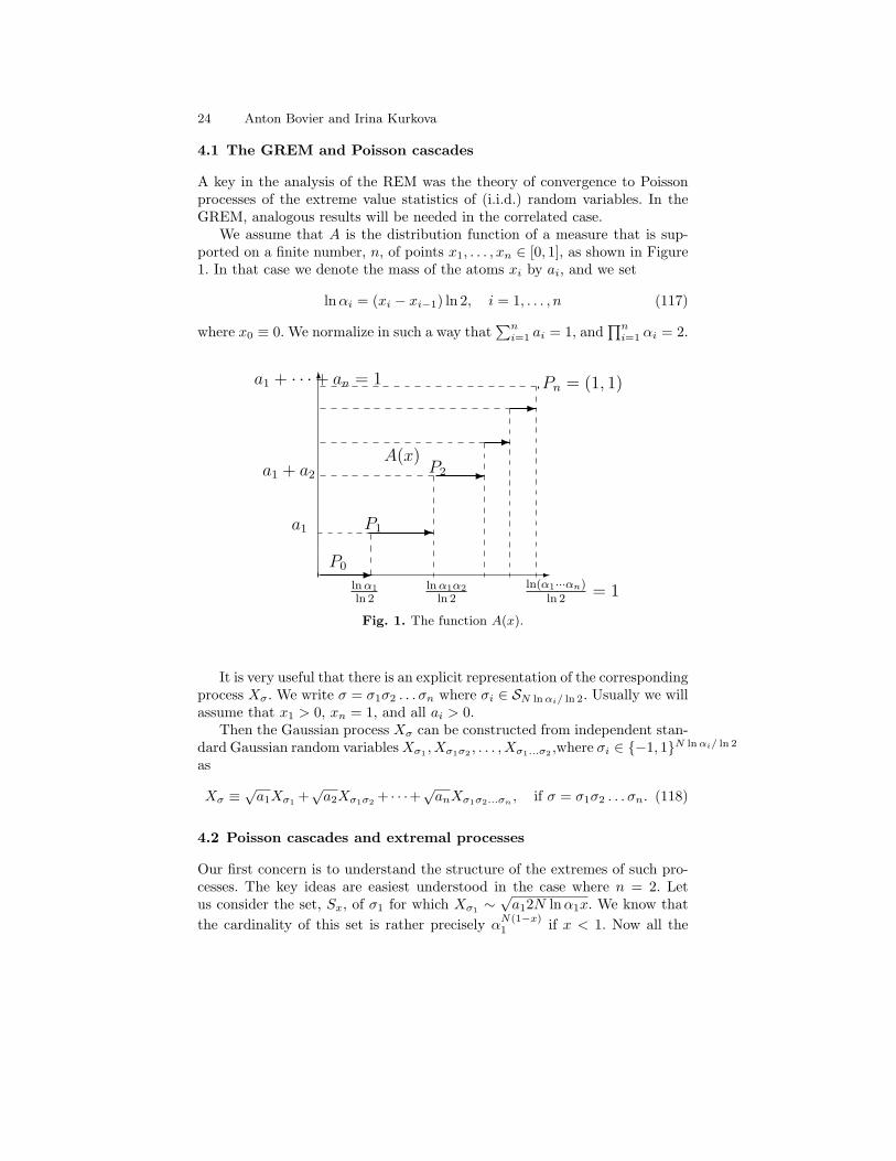
We assume that A is the distribution function of a measure that is sup-ported on a finite number, n, of points x1, . . . , xn ∈ [0, 1], as shown in Figure1. In that case we denote the mass of the atoms xi by ai, and we set

lnαi = (xi − xi−1) ln 2, i = 1, . . . , n (117)

where x0 ≡ 0. We normalize in such a way that∑ni=1 ai = 1, and

∏ni=1 αi = 2.

-

-

-

-

6

--

Pn = (1, 1)

A(x)

P1

P2

lnα1α2

ln 2ln(α1···αn)

ln 2= 1

a1 + · · ·+ an = 1

a1

a1 + a2

lnα1

ln 2

P0

Fig. 1. The function A(x).

It is very useful that there is an explicit representation of the correspondingprocess Xσ. We write σ = σ1σ2 . . . σn where σi ∈ SN lnαi/ ln 2. Usually we willassume that x1 > 0, xn = 1, and all ai > 0.

Then the Gaussian process Xσ can be constructed from independent stan-dard Gaussian random variablesXσ1 , Xσ1σ2 , . . . , Xσ1...σ2 ,where σi ∈ {−1, 1}N lnαi/ ln 2

as

Xσ ≡√a1Xσ1 +

√a2Xσ1σ2 + · · ·+

√anXσ1σ2...σn , if σ = σ1σ2 . . . σn. (118)

4.2 Poisson cascades and extremal processes

Our first concern is to understand the structure of the extremes of such pro-cesses. The key ideas are easiest understood in the case where n = 2. Letus consider the set, Sx, of σ1 for which Xσ1 ∼

√a12N lnα1x. We know that

the cardinality of this set is rather precisely αN(1−x)1 if x < 1. Now all the


αN(1−x)1 αN2 = 2Nα−xN1 random variables Xσ1σ2 with σ1 ∈ Sx are indepen-

dent, so that we know that their maximum is roughly√

2a2N(ln 2− x lnα1).Hence, the maximum of the Xσ with σ1 ∈ Sx is√

a12N ln a1x+√

2a2N(ln 2− x lnα1) (119)

Finally, to determine the overall maximum, it suffices to find the value of xthat maximizes this quantity, which turns out to be given by x∗ = a1 ln 2

lnα1,

provided the constraint a1 ln 2lnα1

< 1 is satisfied. In that case we also find that√a12N ln a1x+

√2a2N(ln 2− x∗ lnα1) =

√2 ln 2 (120)

i.e. the same value as in the REM. On the other hand, if a1 ln 2lnα1

> 1, themaximum is realized by selecting the largest values in the first generation,corresponding to x = 1, and then for each of them the extremal membersof the corresponding second generation. The value of the maximum is then(roughly) √

a12N ln a1 +√

2a2N lnα2 ≤√

2 ln 2 (121)

where equality holds only in the borderline case a1 ln 2lnα1

= 1, which requiresmore care. The condition a1 ln 2

lnα1< 1 has a nice interpretation: it simply means

that the function A(x) < x, for all x ∈ (0, 1).In terms of the point processes, the above considerations suggest the fol-

lowing picture (which actually holds true): If a1 ln 2lnα1

< 1, the point process∑σSN

δu−1N (Xσ) → P (122)

exactly as in the REM, while in the opposite case this process would surelyconverge to zero. On the other hand, we can construct (in both cases) anotherpoint processes, ∑

σ=σ1σ2∈{−1,+1}Nδ√a1u

−1lnα1,N

(Xσ1+√a2u−1lnα2,N

(Xσ1σ2 ) (123)

where we setuα,N (x) ≡ uN lnα/ ln 2(x) (124)

This point process will converge to a process obtained from a Poisson cascade:The process ∑

σ1∈{−1,+1}lnα1N

δu−1α1,N

(Xσ1 ) (125)

converges to a Poisson point process, and, for any σ1, so do the point processes∑σ2∈{−1,+1}lnα2N

δu−1α2,N

(Xσ1σ2 ) (126)


Then the two-dimensional point process∑σ=σ1σ2∈{−1,+1}N

δ(u−1α1,N

(Xσ1 ),u−1α2,N

(Xσ1σ2 )) (127)

converges to a Poisson cascade in R2: we place the Poisson process (alwayswith intensity measure e−xdx) on R, and then, for each atom, we place anindependent PPP on the line orthogonal to the first line that passes throughthat atom. Adding up the atoms of these processes with the right weight yieldsthe limit of the process defined in (123). Now this second point process doesnot yield the extremal process, as long as the first one exists, i.e. as long asthe process (122) does not converge to zero. Interestingly, when we reach theborderline, the process (122) converges to the PPP with intensity Ke−xdxwith 0 < K < 1, while the cascade process yields points that differ from thoseof this process only in the sub-leading order.

Having understood the particular case of two levels, it is not difficult tofigure out the general situation.

The next result tells us which Poisson point processes we can construct.

Theorem 1. Let 0 < ai < 1, αi > 1, i = 1, 2, . . . , n with∑ni=1 ai = 1. Set

α ≡∏ni=1 αi. Then the point process∑

σ=σ1...σn∈{−1,+1}N ln α/ ln 2

δu−1α,N (

√a1Xσ1+

√a2Xσ1σ2+···+√anXσ1σ2...σn ) (128)

converges weakly to the Poisson point process P on R with intensity measureKe−xdx, K ∈ R, if and only if, for all i = 2, 3, . . . , n,

ai + ai+1 + · · ·+ an ≥ ln(αiαi+1 · · ·αn)/ ln α (129)

Furthermore, if all inequalities in (129) are strict, then the constant K = 1.If some of them are equalities, then 0 < K < 1.

Remark 3. An explicit formula for K can be found in [6].

Remark 4. The conditions (129) can be expressed as A(x) ≤ x for all x ∈(0, 1).

Theorem 2. Let αi ≥ 1, and set α ≡∏ki=1 αi. Let Yσ1 , Yσ1σ2 ,

. . . , Yσ1...σk be identically distributed random variables, such that the vectors(Yσ1)σ1∈{−1,1}N lnα1/ ln α , (Yσ1σ2)σ2∈{−1,1}N lnα2/ ln α , . . . . . . . . . ,(Yσ1σ2...σk)σk∈{−1,1}N lnαk/ ln α are independent. Let vN,1(x), . . . , vN,k(x) be func-tions on R such that the following point processes∑

σ1

δvN,1(Yσ1 ) → P1∑σ2

δvN,2(Yσ1σ2 ) → P2 ∀σ1

· · ·∑σk

δvN,k(Yσ1σ2...σk ) → Pk ∀σ1 . . . σk−1 (130)


converge weakly to Poisson point processes, P1, . . . ,Pk, on R with intensitymeasures K1e

−xdx, . . . ,Kke−xdx, for some constants K1, . . . ,Kk. Then the

point processes on Rk,

P(k)N ≡

∑σ1

δvN,1(Yσ1 )

∑σ2

δvN,2(Yσ1σ2 ) · · ·∑σk

δvN,k(Yσ1σ2...σk ) → P(k) (131)

converge weakly to point processes P(k) on Rk, called Poisson cascades with klevels.

Poisson cascades are best understood in terms of the following iterativeconstruction. If k = 1, it is just a Poisson point process on R with intensitymeasure K1e

−xdx. To construct P(2) on R2, we place the process P(1) fork = 1 on the axis of the first coordinate and through each of its points draw astraight line parallel to the axis of the second coordinate. Then we put on eachof these lines independently a Poisson point process with intensity measureK2e

−xdx. These points on R2 form the process P(2). This procedure is nowsimply iterated k times.

Theorems 1 and 2 combined tell us which are the different point processesthat may be constructed in the GREM.

Theorem 3. Let αi ≥ 1, 0 < ai < 1, such that∏ni=1 αi = 2,

∑ni=1 ai = 1. Let

J1, J2, . . . , Jm ∈ N be the indices such that 0 = J0 < J1 < J2 < · · · < Jm = n.We denote by al ≡

∑Jli=Jl−1+1 ai, αl ≡

∏Jli=Jl−1+1 αi, l = 1, 2, . . . ,m, and set

Xσ1...σJl−1σJl−1+1σJl−1+2···σJl ≡

1√al

Jl−Jl−1∑i=1

√aJl−1+iXσJ1 ...σJl−1+i (132)

To a partition J1, J2, . . . , Jm, we associate the function AJ obtained byjoining the sequence of straight line segments going from (xJi , A(xJi) to(xJ+1i , A(x[Ji+1), i = 0,m − 1. A partition is admissible, if A(x) ≤ AJ(x),for all x ∈ [0, 1]. Then, for any admissible partition, the point process

P(m)N ≡

∑σ1...σJ1

δu−1α1,N

(Xσ1...σJ1)

∑σJ1+1...σJ2

δu−1α2,N

(Xσ1...σJ1σJ1+1......σJ2

)· · ·

· · ·∑

σJm−1+1...σJm

δu−1αm,N

(Xσ1...σJm−1σJm−1+1...σJm

)(133)

converges weakly to the process P(m) on Rm defined in Theorem 2 with con-stants K1, . . . ,Km. If AJ(x) < A(x), for all x ∈ (xJi , xJi+1), then

Kl = 1 (134)

Otherwise 0 < Kl < 1.


6

-

-

-

��

-

-

---"

"""

""

��

-

PJ2

PJm = (1, 1)

PJ1a1

A(x)

A(x)

ln(α1α2)ln 2

PJ0ln α1

ln 2= q1 = q2= q0

a1 + a2

ln(α1···αm)ln 2

= 1

a1 + · · ·+ am = 1

Fig. 2. The concave hull of A(x).

Having constructed all possible point processes, we now find the extremalprocess by choosing the one that yields the largest values. It is easy to see thatthis is achieved if as many intermediate hierarchies as possible are groupedtogether. In terms of the geometrical construction just described, this meansthat we must choose the partition J in such a way that the function AJ hasno convex pieces, i.e. that AJ is the concave hull, A, of the function A (seeFig. 2). (The concave hull, A, of a function A is the smallest concave functionsuch that A(x) ≥ A(x), for all x in the domain considered.) Algorithmically,this is achieved by setting J0 ≡ 0, and

Jl ≡ min{J > Jl−1 : AJl−1+1,J > AJ+1,k ∀k ≥ J + 1} (135)

where Aj,k ≡∑ki=j ai/(2 ln(

∏ki=j αi)).

Set γl ≡√al/√

2 ln αl, l = 1, 2, . . . ,m. Clearly, by (135), γ1 > γ2 > · · · >γm. Define the function UJ,N by

UJ,N (x) ≡m∑l=1

(√2Nal ln αl −N−1/2γl(ln(N(ln αl)) + ln 4π)/2

)+ N−1/2x (136)

and the point process

EN ≡∑

σ∈{−1,1}NδU−1

J,N (Xσ) (137)

Theorem 4. (i) The point process EN converges weakly, as N ↑ ∞, to thepoint process on R


E ≡∫

RmP(m)(dx1, . . . , dxm)δ∑m

l=1 γlxl(138)

where P(m) is the Poisson cascade introduced in Theorem 3 correspondingto the partition J1, . . . , Jm given by (135).

(ii)E exists, since γ1 > · · · > γm. It is the cluster point process on R containingan a.s. finite number of points in any interval [b,∞), b ∈ R. The probabilitythat there exists at least one point of E in the interval [b,∞) is decreasingexponentially, as b ↑ ∞.

The formal proofs of these theorems can be found in [6].

4.3 Convergence of the partition function

We will now turn to the study of the Gibbs measures. Technically, the mainstep in the proof will be to show that the infinite-volume limit of the properlyrescaled partition function can be expressed as a certain functional of Poissoncascade processes, as suggested by Ruelle [25].

For any sequence of indices, Ji, such that the function AJ is concave, thepartition function can be written as:

Zβ,N = e∑mj=1

(βN√

2aj ln αj−βγj [ln(N ln αj)+ln 4π]/2)× (139)

Eσ1...σJ1eβγ1u

−1α1,N

(Xσ1...σJ1) · · ·EσJm−1+1...σJm

eβγmu

−1αm,N

(Xσ1...σJm−1σJm−1+1...σJm

)

Clearly, not all of these representations can be useful, i.e the sums in the sec-ond line should converge to a finite random variable. For this to happen, fromwhat we learned in the REM, each of the sums should be at ‘low temperature’,meaning here that βγ` > 1. Moreover, we should expect that there is a rela-tion to the maximum process; in fact, this will follow from the condition thatγi > γi+1, for all i that appear. Thus we will have to choose the partition Jthat yields the extremal process, and we have to cut the representation (140)at some temperature-dependent level, Jl(β), and treat the remaining hierar-chies as high-temperature REM’s, i.e. replace them by their mean value. Thelevel l(β) is determined by

l(β) ≡ max{l ≥ 1 : βγl > 1} (140)

and l(β) ≡ 0 if βγ1 ≤ 1.From these considerations it is now very simple to compute the asymptotics

of partition function. The resulting formula for the free energy was first foundin [9]:

Theorem 5. [9] With the notation introduced above,

limN→∞

Φβ,N = β

l(β)∑i=1

√2ai ln αi +

n∑i=Jl(β)+1

β2ai/2, a.s. (141)


The condition that for β ≤ βc, l(β) = 0, defines the critical temperature,βc = 1/γ1.

The more precise asymptotics of the partition function is as follows.

Theorem 6. Let J1, J2, . . . , Jm ∈ N, be the sequence of indices defined by(135) and l(β) defined by (140). Then, with the notations introduced above,

e−β∑l(β)j=1

(N√

2aj ln αj−γj [ln(N ln αj)+ln 4π]/2)−Nβ2∑n

i=Jl(β)+1 ai/2Zβ,N

D→ C(β)∫

Rl(β)eβ∑l(β)i=1 γixiP(l(β))(dx1 . . . dxl(β)) (142)

This integral is over the process P(l(β)) on Rl(β) from Theorem 2 with constantsKj from Theorem 3. The constant C(β) satisfies

C(β) = 1, ifβγl(β)+1 < 1, (143)

and 0 < C(β) < 1, otherwise.

Remark 5. An explicit formula for C(β) is given in [6].

The integrals over the Poisson cascades appearing in Theorem 6 are to beunderstood as∫

Rmeβγ1x1+···+βγmxmP(m)(dx1 . . . dxm) (144)

≡ limx↓−∞

∫(x1,...,xm)∈Rm,

∃i,1≤i≤m:γ1x1+···+γixi>(γ1+···+γi)x

eβγ1x1+···+βγmxmP(m)(dx1 . . . dxm)

The existence of these limits requires the conditions on the γi mentionedbefore, and thus can be seen as responsible for the selection of the partitionJ and the cut-off level l(β). Namely [6]:

Proposition 2. Assume that γ1 > γ2 > . . . > γm > 0, and βγm > 1. Then

(i) For any a ∈ R the process P(m) contains a.s. a finite number of points(x1, . . . , xm) such that γ1x1 + · · ·+ γmxm > a.

(ii)The limit in (144) exists and is finite a.s.

4.4 The asymptotic model

As in the REM, we are able to reinterpret the convergence of the partitionfunction in terms of an asymptotic statistical mechanics model.

This time, it has the following ingredients:

• State space: N`, that should be though of as an `-level tree with infinitebranching number;

• A sequence,γ ≡ (γ1 > γ2 > · · · > γ`) of numbers;


• Random Hamiltonian: H`γ : N` → R, where

H`γ =∑k=1

γkxik , (145)

and xik is the ik-th atom of the Poisson process P(k);• Temperature: 1/β;• Partition function: Zβ =

∑i∈N` e

βH(i);• Gibbs measure:

µ`β,γ(i) = Z`βeβH`γ(i). (146)

Our convergence results so far can be interpreted in terms of this modelas follows:

• The partition function of the GREM converges, after multiplication withthe correct scaling factor, to Zβ ;

A new feature compared to the situation in the REM is that that state spaceN` of the asymptotic model carries a natural non-trivial distance, namely thehierarchical distance, respectively the corresponding hierarchical overlap

d(i, j) =1`

(min(k : ik 6= jk)− 1). (147)

This allows to define in the asymptotic model the analog of the local massdistribution (see (106) as

φβ(i, t) ≡ µβ (d(i, j) > t) . (148)

This allows also to write the empirical distance distribution function for theasymptotic model in in the form

Kβ ≡∑i∈N`

µβ(i)δφβ(i,·) (149)

Clearly we expect Kβ to be related to the analogous object in the GREM, i.e.to Kβ,N defined as in (114). The only additional ingredient is a translationbetween the overlap on the hypercube and the tree-overlap (148). This is infact given by the following Lemma:

Lemma 11. Let

q` ≡∑n=1

ln αnln 2

, (150)

and let f(q) ≡ sup{k : qk ≤ q}/`(β). For any β, for q ≤ qmax ≡ q`(β),

limN↑∞

µ⊗2β,N (RN (σ, σ′) ≤ q) = µ⊗2

β (d(i, j) ≤ f(q)) . (151)


A nontrivial aspect of the lemma above is that the overlap defined in termsof the non-hierarchical RN is asymptotically given in terms of the distributionof a hierarchical overlap, d. In fact, it would be quite a bit easier to show that

limN↑∞

µ⊗2β,N (dN (σ, σ′) ≤ q) = µ⊗2

β (d(i, j) ≤ f(q)) . (152)

where dN is defined in (54). The fact that the two distances are asymptoticallythe same on the support of the Gibbs measures is remarkable and the simplestinstance of the apparent universality of ultrametric structures in spin glasses.Bolthausen and Kistler [5] (see also Jana [20]) have shown that the sameoccurs in a class of models where the covariance depends on several differenthierarchical distances.

The main result on the limiting Gibbs measures can now be formulated asfollows:

Theorem 7. Under the assumptions and with the notation of Lemma (11)

limN↑∞Kβ,N = Kfβ , (153)

where f : [0, qmax]→ [0, 1] is defined in Lemma 11 and

Kfβ =∑i∈N`

µβ(i)δφβ(i,f(·)). (154)

We see that in the aysmptotic model, we have so far three ingredients: 1)the Poisson cascade; 2) the weights γi; 3) the mapping f from that readjuststhe tree-distance.

In fact, Kβ as a probability distribution on distributions of distances con-tains a lot of gauge invariance. In particular, neither the measures µβ nor theunderlying space N` play a particular role. In fact, there is a canonical way toshift all the structure into the ultrametric and to chose as a canonical spacethe interval [0, 1] and as a canonical measure on it the Lebesgue measure. Todo this, chose a one-to-one map,

θ : N` → [0, 1] (155)

such that for any Borel set, A ⊂ B([0, 1],

|A| = µβ(θ−1(A)). (156)

Then define the overlap, γ1, on [0, 1], by

γ1(x, y) = f−1(d(θ−1(x), θ−1(y)

)). (157)

Note that this overlap structure is now random, and in fact contains all theremaining randomness of the system. Then we can write Kfβ as


Kfβ =∫ 1

0

dxδ|{y:γ1(x,y)>·}|. (158)

This representation allows, in fact, to put all GREMs on a single footing.Namely, one can show that the random overlaps γ1 can all be obtained bya deterministic time change from the genealogical distance of a particularcontinuous time branching process, the so-called Neveu CBP. This observationgoes back to an unpublished paper of Neveu [24] and was elaborated on byBertoin and LeGall [3] and the present authors [8].

5 Gaussian comparison and applications

We now return to the study of the SK type models. We will emphasize herethe role of classical comparison results for Gaussian processes. A clever use ofthem will allow to connect the SK models with the GREMs discussed above.We begin by recalling the basic comparison theorem.

5.1 A theorem of Slepian-Kahane

Lemma 12. Let X and Y be two independent n-dimensional Gaussian vec-tors. Let D1 and D2 be subsets of {1, . . . , n} × {1, . . . , n}. Assume that

EXiXj ≤ EYiYj , if (i, j) ∈ D1

EXiXj ≥ EYiYj , if (i, j) ∈ D2 (159)EXiXj = EYiYj , if (i, j) 6∈ D1 ∪D2

Let f be a function on Rn, such that its second derivatives satisfy

∂2

∂xi∂xjf(x) ≥ 0, if (i, j) ∈ D1

∂2

∂xi∂xjf(x) ≤ 0, if (i, j) ∈ D2 (160)

ThenEf(X) ≤ Ef(Y ) (161)

Proof. The first step of the proof consists of writing

f(X)− f(Y ) =∫ 1

0

dtd

dtf(Xt) (162)

where we define the interpolating process

Xt ≡√tX +

√1− t Y (163)


Next observe that

d

dtf(Xt) =

12

n∑i=1

∂

∂xif(Xt)

(t−1/2Xi − (1− t)−1/2Yi

)(164)

Finally, we use the generalization of the standard Gaussian integration byparts formula to the multivariate setting, namely:

Lemma 13. Let Xi, i ∈ {1, . . . , n} be a multivariate Gaussian process, andlet g : Rn → R be a differentiable function of at most polynomial growth. Then

Eg(X)Xi =n∑j=1

E(XiXj)E∂

∂xjg(X) (165)

Applied to the mean of the left-hand side of (164) this yields

Ef(X)− Ef(Y ) =12

∑i,j

∫0,1

dt (EXiXj − EYiYj) E∂2

∂xj∂xif(Xt) (166)

from which the assertion of the theorem can be read off.

Note that Equation (166) has the flavor of the fundamental theorem ofcalculus on the space of Gaussian processes.

5.2 The thermodynamic limit through comparison

Theorem 8. [17] Assume that Xσ is a normalized Gaussian process on SNwith covariance

EXσXτ = ξ(RN (σ, τ)) (167)

where ξ : [−1, 1]→ [0, 1] is convex and even. Then

limN↑∞

−1βN

E ln Eσeβ√NXσ ≡ fβ (168)

exists.

Proof. The proof of this fact is frightfully easy, once you think about us-ing Theorem 12. Choose any 1 < M < N . Let σ = (σ, σ) where σ =(σ1, σ2, . . . , σM ), and σ = (σM+1, . . . , σN ). Define independent Gaussian pro-cesses X and X on SM and SN−M , respectively, such that

EXσXτ = ξ(RM (σ, τ)) (169)

andEXσXτ = ξ(RN−M (σ, τ) (170)

Set


Yσ ≡√

MN Xσ +

√N−MN Xσ (171)

Clearly,

EYσYτ = MN ξ(RM (σ, τ)) + N−M

N ξ(RN−M (σ, τ)) (172)

≥ ξ(MN RM (σ, τ) + N−M

N (RN−M (σ, τ)))

= ξ(RN (σ, τ))

Define real-valued functions FN (x) ≡ ln Eσeβ√Nxσ on R2N . It is straightfor-

ward thatEFN (Y ) = EFM (X) + EFN−M (X) (173)

A simple computation shows that, for σ 6= τ ,

∂2

∂xσ∂xτFN (x) = −2−2Nβ2Neβ

√N(xσ+xτ )

Z2β,N

≤ 0 (174)

Thus, Theorem 12 tells us that

EFN (X) ≥ EFN (Y ) = EFM (X) + EFN−M (X) (175)

This implies that the sequence −EFN (X) is subadditive, and this in turnimplies (see Section 1.2) that the free energy exists , provided it is bounded,which is easy to verify (see e.g. the discussion on the correct normalization inthe SK model).

The same ideas can be used for other types of Gaussian processes, e.g. theGREM-type models discussed above [10].

Convergence of the free energy in mean implies readily almost sure con-vergence. This follows from a general concentration of measure principle forfunctions of Gaussian random variables.

5.3 An extended comparison principle.

As I have mentioned, comparison of the free energy of SK models to simplermodels do not immediately seem to work. The idea is to use comparison on amuch richer class of processes. Basically, rather than comparing one processto another, we construct an extended process on a product space and usecomparison on this richer space. Let us first explain this in an abstract setting.We have a process X on a space S equipped with a probability measure Eσ.We want to compute as usual the average of the logarithm of the partitionfunction F (X) = ln EσeβXσ . Now consider a second space T equipped witha probability law Eα. Choose a Gaussian process, Y , independent of X, onthis space, and define a further independent process, Z, on the product spaceS×T . Define real valued functions, G,H, on the space of real valued functionson T and S×T , respectively, via G(y) ≡ ln Eαeβyα and H(z) = ln EσEαeβzσ,α .Note that H(X+Y ) = F (X)+G(Y ). Assume that the covariances are chosensuch that


cov(Xσ, Xσ′) + cov(Yα, Yα′) ≥ cov(Zσ,α, Zσ′,α′) (176)

Since we know that the second derivatives of H are negative, we get fromTheorem 12 that

EF (X) + EG(Y ) = EH(X + Y ) ≤ EH(Z) (177)

This is a useful relation if we know how to compute EG(Y ) and EH(Z). Thisidea may look a bit crazy at first sight, but we must remember that we havea lot of freedom in choosing the auxiliary spaces and processes to our con-venience. Before turning to the issue whether we can find useful computableprocesses Y and Z, let us see why we could hope to find in this way sharpbounds.

5.4 The extended variational principle and thermodynamicequilibrium

To do so, we will show that, in principle, we can represent the free energyin the thermodynamic limit in the form EH(Z) − EG(Y ). To this end letS = SM and T = SN , both equipped with their natural probability measureEσ. We will think of N � M , and both tending to infinity eventually. Wewrite again S × T 3 σ = (σ, σ). Consider the process Xσ on SN+M withcovariance ξ(RN+M (σ, σ′)). We would like to write this as

Xσ = Xσ + Xσ + Zσ (178)

where all three processes are independent. Note that here and in the sequelequalities between random variables are understood to hold in distribution.Moreover, we demand that

cov(Xσ, Xσ′) = ξ( MN+MRM (σ, σ′)) (179)

andcov(Xσ, Xσ′) = ξ( N

N+MRN (σ, σ′)) (180)

Obviously, this implies that

cov(Zσ, Zσ′) = ξ(

MN+MRM (σ, σ′) + N

N+MRN (σ, σ′))

(181)

− ξ(

MN+MRM (σ, σ′)

)− ξ

(N

N+MRN (σ, σ′))

(we will not worry about the existence of such a decomposition; if ξ(x) =xp, we can use the explicit representation in terms of p-spin interactions toconstruct them). Now we first note that, by super-additivity [2]

limM↑∞

1βM

lim infN↑∞

E logZβ,N+M

Zβ,N= −fβ (182)


Thus we need a suitable representation for Zβ,N+MZβ,N

. But

Zβ,N+M

Zβ,N=

Eσeβ√N+M(Xσ+Zσ+Xσ)

Eσeβ√N+M

(√(1−M/(N+M))Xσ

) (183)

Now we want to express the random variables in the denominator in the form√(1−M/(N +M))Xσ = Xσ + Yσ (184)

where Y is independent of X. Comparing covariances, this implies that

cov(Yσ, Yσ′) = (1−M/(N +M))ξ(RN (σ, σ′))

− ξ(

NN+MRN (σ, σ′)

)(185)

As we will be interested in taking the limit N ↑ ∞ before M ↑ ∞, we mayexpand in M/(N +M) to see that to leading order in M/(N +M),

cov(Yσ, Yσ′) ∼ MN+MRN (σ, σ′)ξ′

(N

N+MRN (σ, σ′))

− MN+M ξ

(N

N+MRN (σ, σ′))

(186)

Finally, we note that the random variables Xσ are negligible in the limitN ↑ ∞, since their variance is smaller than ξ(M/(N + M)) and hence theirmaximum is bounded by

√ξ(M/(N +M))M ln 2, which even after multipli-

cation with√N +M gives no contribution in the limit if ξ tends to zero faster

than linearly at zero, which we can safely assume. Thus we see that we canindeed express the free energy as

fβ = − limM↑∞

lim infN↑∞

1βM

E lnEσEσeβ

√N+MZσ,σ

Eσeβ√N+MYσ

(187)

where the measure Eσ can be chosen as a probability measure defined byEσ(·) = Eσeβ

√N+MXσ (·)/Zβ,N,M where Zβ,N,M ≡ Eσeβ

√N+MXσ . Of course

this representation is quite pointless, because it is certainly uncomputable,since E is effectively the limiting Gibbs measure that we are looking for. How-ever, at this point there occurs a certain miracle: the (asymptotic) covariancesof the processes X,Y, Z satisfy

ξ(x) + yξ′(y)− ξ(y) ≥ xξ′(y) (188)

for all x, y ∈ [−1, 1], if ξ is convex and even. This comes as a surprise, sincewe did not do anything to impose such a relation! But it has the remarkableconsequence that asymptotically, by virtue of Lemma 12 it implies the bound

E ln Eσeβ√MXσ ≤ E ln

EσEσeβ√N+MZσ,σ

Eσeβ√N+MYσ

(189)


(if the processes are taken to have the asymptotic form of the covariances).Moreover, this bound will hold even if we replace the measure E by some otherprobability measure, and even if we replace the overlap RN on the space SNby some other function, e.g. the ultrametric dN . Seen the other way around,we can conclude that a lower bound of the form (177) can actually be made asgood as we want, provided we choose the right measure E. This observation isdue to Aizenman, Sims, and Starr [2]. They call the auxiliary structure madefrom a space T , a probability measure Eα on T , a normalized distance q onT , and the corresponding processes, Y and Z, a random overlap structure

cov(Yα, Yα′) = q(α, α′)ξ′(q(α, α′))− ξ(q(α, α′)) (190)

and the process Zσ,α on SN × [0, 1] with covariance

cov(Zσ,α, Zσ′,α′) ≡ RN (σ, σ′)ξ′(q(α, α′)) (191)

With these choices, and naturally Xσ our original process with covarianceξ(RN ), the equation (176) is satisfied, and hence the inequality (177) holds,no matter what choice of q and Eα we make. Restricting these choices tothe random genealogies obtained from Neveu’s process by a time change withsome probability distribution function m, and Eα the Lebesgue measure on[0, 1], gives the bound we want.

This bound would be quite useless if we could not compute the right-handside. Fortunately, one can get rather explicit expressions. We need to computetwo objects:

EαEσeβ√NZσ,α (192)

andEαeβ

√NYα (193)

In the former we use that Z has the representation

Zσ,α = N−1/2N∑i=1

σizα,i (194)

where the processes zα,i are independent for different i and have covariance

cov(zα,i, zα′,i) = ξ′(q(α, α′)) (195)

Thus at least the σ- average is trivial:

EαEσeβ√NZσ,α = Eα

N∏i=1

eln cosh(βzα,i) (196)

Thus we see that, in any case, we obtain bounds that only involve objects thatwe introduced ourselves and that thus can be manipulated to be computable.In fact, such computations have been done in the context of the Parisi solution[23]. A useful mathematical reference is [4].

This is the form derived in Aizenman, Sims, and Starr [2].


5.5 Parisi auxiliary systems

The key idea of the Parisi solution is to chose as an auxiliary system as theasymptotic model of the GREM.

That is, the space T in this case is chosen as a n-level infinite tree Nnequipped with the measure µβ defined in (146).T is naturally endowed with its tree overlap, d(i, j) ≡ n−1(min{` : i` 6=

j`} − 1). This distance will play the role of the distance q on T . Finally, wedefine the processes Yi and Zi,σ with covariances

cov(Yi, Yj) = d(i, j)ξ′(d(i, j))− ξ(d(i, j)) ≡ h(d(i, j)) (197)

and the process Zσ,i on SN × T with covariance

cov(Zσ,j , Zσ′,j) ≡ RN (σ, σ′)ξ′(d(i, j)) (198)

It is easy to see that such processes can be constructed as long as h, ξ′ areincreasing functions. E.g.

Yi =n∑`=1

√h(`/n)− h((`− 1)/n)Y (`)

i1...i`(199)

where Y (`)i1...i`

are independent standard normal random variables. In this way,we have constructed an explicit random overlap structure, which correspondsindeed to the one generating the Parisi solution.

Note that also the auxiliary structure depends only on the information con-tained in the empirical distance distribution, Kβ , associated with the asymp-totic model. In fact we could alternatively use T = [01] equipped with theLebesgue measure and the random overlap γ1, as defined in (158). While thisis nice conceptually, for actual computations the form above will be moreuseful, however.

5.6 Computing with Poisson cascades

Lemma 14. Assume that P be a Poisson process with intensity measuree−xdx. and let Zi,j, i ∈ N, j ∈ N and Y be iid standard normal randomvariables. Let gj : R → R, j = 1, . . . ,M , be smooth functions, such that, forall |m| ≤ 2, there exist C <∞, independent of N , such that

EY emgi(Y ) ≡ eLi(m) < C (200)

Let xi be the atoms of the Poisson process P with intensity measure e−xdx.Then

E ln∑∞i=1 e

αxi+∑Mj=1 gj(Zi,j)∑∞

i=1 eαxi

=M∑j=1

αLj(1/α). (201)


Proof. Let for simplicity M = 1. The numerator on the left in (201) can bewritten as ∫

eαzP(dz)

where P is the point process

P ≡∑j

δzj+α−1g(Yj)

This follows from a general fact about Poisson point processes: if N ≡∑i δxi

is a Poisson point process with intensity measure λ on E, and Yi are iidrandom variables with distribution ρ, then

N ≡∑i

δxi+Yi

is a Poisson process with intensity measure λ ∗ ρ on the set E + suppρ. Thisfollows from the representation of N as

N =Nλ∑i=1

δXi

where Nλ is Poisson with parameter∫Eλ(dx) ≡ |λ| (if this is finite), and Xi

iid random variables with distribution λ/|λ|. Clearly

N =∑i

δxi+Yi =Nλ∑i=1

δXi+Yi

is again of the form of a PPP, and the distribution of Xi + Yi is λ ∗ ρ/|λ|.Since the total intensity of the process is the parameter of Nλ, |λ|, it followsthat the intensity measure of this process is the one we claimed.

Thus, in our case, P is a PPP whose intensity measure is the convolutionof the measure e−zdz and the distribution of the random variable α−1g(Y ).A simple computation shows that this is EY eg(Y )/αe−zdz, i.e. a multiple ofthe original intensity measure!

Finally, one makes the elementary but surprising and remarkable obser-vation that the Poisson point process

∑j δz+ln EY eg(Y )/α has the same intensity

measure, and therefore,∑j eαzj+g(Yj) has the same law as

∑j eαzj [EY eg(Y )/α]α:

multiplying each atom with an iid random variable leads to the same processas multiplying each atom by a suitable constant! The assertion of the Lemmafollows immediately.

Remark 6. Nobody seems to know who made this discovery. Michael Aizen-man told me about it and attributed to David Ruelle, but one cannot find itin his paper. A slightly different proof from the one above can be found in[26].


Let us look first at (193). We can then write∑i

eHnγ(i+β

√MYi =

∑i

eHnγ(i)+β

√MYin−1+

√h(xn)−h(xn−1)Y

(n)i

=∑

i1...in−1

e∑n−1`=1 γ`xi1...σ`+β

√MYin−1

×∑in

eγnxin−1,in+β

√M√h(1)−h(1−1/n)Y

(n)in−1,in (202)

Using Lemma 14, the last factor can be replaced by

Eineγnxin−1,in+β

√M√h(1)−h(1−1/n)Y

(n)in−1,in (203)

→[∫

dz√2πe−

z22 ezmnβ

√M√h(1)−h(1−1/n)

]1/mn∑in

eγnxi (204)

= eβ2M

2 mn(h(1)−h(1−1/n))∑in

eγnxi (205)

(we use throughout mn = 1/γn). Note that the last factor is independent ofthe random variables xi1,...,i` with ` < n. Thus

E ln∑i

eαxi+β√MYi = E ln

∑i1,...,in−1

e∑n−1`=1 γ`xi1,...,in−1+β

√MYi1,...,in−1

+β2M

2mn(h(1)− h(1− 1/n)) + E ln

∑in

eγnxi (206)

The first term now has the same form as the original one with n replaced byn − 1, and thus the procedure can obviously iterated. As the final result, weget that a consequence, we get that

M−1E ln∑i exi+β

√MYi∑

i exi

=n∑`=1

β2

2m`(h(1− `/n)− h(1− (`− 1)/n))

=β2

2

∫ 1

0

m(x)xξ′′(x)dx (207)

The computation of the expression (192) is now very similar, but gives amore complicated result since the analogs of the expressions (203) cannot becomputed explicitly. Thus, after the k-th step, we end up with a new functionof the remaining random variables Yi1...in−k . The result can be expressed inthe form


1M

E ln EiEσeβ√MZσ,i = ζ(0, h,m, β) (208)

(here h is the magnetic field (which we have so far hidden in the notation)that can be taken as a parameter of the a priori distribution on the σ suchthat Eσi(·) ≡ 1

2 cosh(βh)

∑σi=±1 e

βhσi(·)) where ζ(1, h) = ln cosh(βh), and

ζ(xa−1, h) =1ma

ln∫

dz√2πe−z

2/2emaζ(xa,h+z√ξ′(xa)−ξ′(x)) (209)

(we put xa = a/n).In all of the preceeding discussion, the choice of the parameter n and of

the numbers mi = 1/γ1 is still free. FromWe can now announce Guerra’s bound in the following form:

Theorem 9. [16] Let ζ(t, h,m, b) be the function defined in terms of the re-cursion (209). Then

limN↑∞

N−1E lnZβ,h,N ≤ infmζ(0, h,m, β)− β2

2

∫ 1

0

m(x)xξ′′(x)dx (210)

where the infimum is over all probability distribution functions m on the unitinterval.

Remark 7. It is also interesting to see that the recursive form of the functionζ above can also be represented in a closed form as the solution of a partialdifferential equation. Consider the case ξ(x) = x2/2. Then ζ is the solution ofthe differential equation

∂

∂tζ(t, h) +

12

(∂2

∂h2ζ(t, h) +m(t)

(∂

∂hζ(t, h)

)2)

= 0 (211)

with final conditionζ(1, h) = ln cosh(βh) (212)

If m is a step function, it is easy to see that a solution is obtained by setting,for x ∈ [xa−1, xa),

ζ(x, h) =1ma

ln Ezemaζ(xa,h+z√xa−x) (213)

For general convex ξ, analogous expressions can be obtained through changesof variables [16].

5.7 Talagrand’s theorem

In both approaches, it pays to write down the expression of the differencebetween the free energy and the lower bound, since this takes a very suggestiveform.


To do this, we just have to use formula (166) with

Xtσ,α ≡

√t(Xσ + Yα) +

√1− tZσ,α (214)

and f(Xt) replaced by H(Xt) = ln EσEαeβ√NZtσ,α . This gives the equality

H(X + Y )−H(Z) =12

E∫ 1

0

dtµ⊗2β,t,N (dσ, dα)

(ξ(RN (σ, σ′))

+ q(α, α′)ξ′(q(α, α′))

− ξ(q(α, α′))−RN (σ, σ′)ξ′(q(α, α′)))

(215)

where the measure µβ,t,N is defined as

µβ,t,N (·) ≡ EσEαeβ√NXtσ,α(·)

EσEαeβ√NXtσ,α

(216)

where we interpret the measure µβ,t,N as a joint distribution on SN × [0, 1].Note that for convex and even ξ, the function ξ(RN (σ, σ′))+q(α, α′)ξ′(q(α, α′))−ξ(q(α, α′)) vanishes if and only if RN (σ, σ′) = q(α, α′). Thus for the left handside of (215) to vanish, the replicated interpolating product measure should(for almost all t), concentrate on configurations where the overlaps in the σ-variables coincide with the genealogical distances of the α-variables. Thus wesee that the inequality in Theorem 9 will turn into an equality if it is possibleto choose the parameters of the reservoir system in such a way that the theoverlap distribution on SN aligns with the genealogical distance distributionin the reservoir once the systems are coupled by the interpolation.

This latter fact was proven very recently, and not long after the discoveryof Guerra’s bound, by M. Talagrand [29].

Theorem 10. [29] Let ζ(t, h,m, b) be the function defined in terms of (211)and (212). Then

limN↑∞

N−1E lnZβ,h,N = infm

(ζ(0, h,m, .β)− β2

2

∫ 1

0

m(x)xξ′′(x)dx)

(217)

where the infimum is over all probability distribution functions m on the unitinterval.

I will not give the complex proof which the interested reader should studyin the original paper [29], but I will make some comments on the key ideas.First, Talagrand proves more than the assertion 217. What he actually provesis the following. For any ε > 0, there exists a positive integer n(ε) < ∞, anda probability distribution function mn that is a step function with n steps,such that for all t > ε,


limN↑∞

Eµ⊗2β,t,N (dσ, dα)

(ξ(RN (σ, σ′)) + q(α, α′)ξ′(q(α, α′))

−ξ(q(α, α′))−RN (σ, σ′)ξ′(q(α, α′)))

= 0 (218)

if the measure µb,t,N corresponds to the genealogical distance obtained fromthis function m. That is to say, if the coupling parameter t is large enough, theSK model can be aligned to a GREM with any desired number of hierarchies.

References

1. R.J. Adler. On excursion sets, tube formulas and maxima of random fields.Ann. Appl. Probab., 10(1):1–74, 2000.

2. M. Aizenman, R. Sims, and S.L. Starr. An extended variational principle forthe SK spin-glass model. Phys. Rev. B, 6821(21):4403–4403, 2003.

3. J. Bertoin and J.-F. Le Gall. The Bolthausen-Sznitman coalescent and the ge-nealogy of continuous-state branching processes. Probab. Theory Related Fields,117(2):249–266, 2000.

4. E. Bolthausen and A.-S. Sznitman. On Ruelle’s probability cascades and anabstract cavity method. Comm. Math. Phys., 197(2):247–276, 1998.

5. Erwin Bolthausen and Nicola Kistler. On a nonhierarchical version of the gen-eralized random energy model. Ann. Appl. Probab., 16(1):1–14, 2006.

6. A. Bovier and I. Kurkova. Derrida’s generalised random energy models. I. Mod-els with finitely many hierarchies. Ann. Inst. H. Poincare Probab. Statist.,40(4):439–480, 2004.

7. A. Bovier and I. Kurkova. Derrida’s generalized random energy models. II.Models with continuous hierarchies. Ann. Inst. H. Poincare Probab. Statist.,40(4):481–495, 2004.

8. A. Bovier and I. Kurkova. Gibbs measures of Derrida’s generalized randomenergy models and genealogies of Neveu’s continuous state branching processe.In Spin glasses, volume 1900 of Lecture Notes in Math. Springer, Berlin, 2007.

9. D. Capocaccia, M. Cassandro, and P. Picco. On the existence of thermodynam-ics for the generalized random energy model. J. Statist. Phys., 46(3-4):493–505,1987.

10. P. Contucci, M. Degli Esposti, C. Giardina, and S. Graffi. Thermodynami-cal limit for correlated Gaussian random energy models. Comm. Math. Phys.,236(1):55–63, 2003.

11. B. Derrida. A generalisation of the random energy model that includes correla-tions between the energies. J. Phys. Lett., 46:401–407, 1985.

12. R.S. Ellis. Entropy, large deviations, and statistical mechanics, volume 271 ofGrundlehren der Mathematischen Wissenschaften [Fundamental Principles ofMathematical Sciences]. Springer-Verlag, New York, 1985.

13. E. Gardner and B. Derrida. Magnetic properties and function q(x) of the gen-eralised random energy model. J. Phys. C, 19:5783–5798, 1986.

14. E. Gardner and B. Derrida. Solution of the generalised random energy model.J. Phys. C, 19:2253–2274, 1986.

15. E. Gardner and B. Derrida. The probability distribution of the partition functionof the random energy model. J. Phys. A, 22(12):1975–1981, 1989.


16. F. Guerra. Broken replica symmetry bounds in the mean field spin glass model.Comm. Math. Phys., 233(1):1–12, 2003.

17. F. Guerra and F. L. Toninelli. The thermodynamic limit in mean field spin glassmodels. Comm. Math. Phys., 230(1):71–79, 2002.

18. E. Ising. Beitrag zur Theorie des Ferro- und Paramagnetismus. Ph.D. thesis,Univ. Hamburg, 1924.

19. E. Ising. Zeitschrift. f. Physik, 31:253, 1925.20. Nabin Kumar Jana. Contributions to random energy models. Thesis, 2008.21. M.R. Leadbetter, G. Lindgren, and H. Rootzen. Extremes and related properties

of random sequences and processes. Springer Series in Statistics. Springer-Verlag,New York, 1983.

22. M. Ledoux and M. Talagrand. Probability in Banach spaces, volume 23 of Ergeb-nisse der Mathematik und ihrer Grenzgebiete (3) [Results in Mathematics andRelated Areas (3)]. Springer-Verlag, Berlin, 1991.

23. M. Mezard, G. Parisi, and M.A. Virasoro. Spin glass theory and beyond, volume 9of World Scientific Lecture Notes in Physics. World Scientific Publishing Co.Inc., Teaneck, NJ, 1987.

24. J. Neveu. A continuous state branching process in relation with the GREMmodel of spin glass theory. rapport interne 267, Ecole Polytechnique Paris,1992.

25. D. Ruelle. A mathematical reformulation of Derrida’s REM and GREM. Comm.Math. Phys., 108(2):225–239, 1987.

26. A. Ruzmaikina and M. Aizenman. Characterization of invariant measures atthe leading edge for competing particle systems. Ann. Probab., 33(1):82–113,2005.

27. D. Sherrington and S. Kirkpatrick. Solvable model of a spin glas. Phys. Rev.Letts., 35:1792–1796, 1972.

28. B. Simon. The statistical mechanics of lattice gases. Vol. I. Princeton Series inPhysics. Princeton University Press, Princeton, NJ, 1993.

29. Michel Talagrand. The Parisi formula. Ann. of Math. (2), 163(1):221–263, 2006.

Index

Aizenman, M., 27

binomial coefficientasymptotics, 5

concentration of measure, 24convexity, 9Cramer entropy, 5Curie, P., 4Curie–Weiss model, 4

distanceultrametric, 13

entropyCramer, 5

ferromagnetism, 2free energy

in SK model, 33of spin system , 2

Gaussianprocess, 13

Gibbs measure, 2Guerra’s bound, 32

integration by partsGaussian

multivariate, 23Ising model, 1Ising, E., 1isotherm, 9

Kirkpatrick, S., 12

large deviationprinciple, 6

mean field models, 4metastate, 20

non-convexity, 9

Parisi solution, 28partition function, 2point process

Poisson, 17Poisson process

of extremes, 18pure state, 20

random overlap structure, 27random process

Gaussian, 13

Sherrington, D., 12Sherrington–Kirkpatrick (SK)-model,

12Sims, R., 27spin

configuration, 1variable, 1

spin-glass, 12Starr, S.L., 27sub-additivity, 24subadditivity, 3

Talagrand’s theorem, 33Talagrand, M., 33

Weiss, P., 4

a short course on mean field spin glasses

Documents