1

A Set-based Approach for Coordination of

Multi-level Collaborative Design Studies

Xin Chen1, Atif Riaz2, Marin D. Guenov3, Arturo Molina-Cristóbal4 Cranfield University, Bedford, Bedfordshire, MK43 0AL, United Kingdom

Presented in this paper is a framework for design coordination of hierarchical (multi-level)

design studies. The proposed framework utilizes margin management and set-based design

principles for handling the challenges associated with vertical and horizontal design

coordination. The former is based on flexible constraints/margins, while the latter is handled

by intersecting feasible design spaces across different teams. The framework is demonstrated

with an industrial test-case from the UK ATI APPROCONE (Advanced PROduct CONcept

analysis Environment) project.

Nomenclature

𝑥𝑙𝑖 = 𝑖𝑡ℎ local variable

𝑥𝑠𝑖 = 𝑖𝑡ℎ shared variable

𝑡𝑖𝑗 = target variable as a requirement of the 𝑖𝑡ℎ subspace and target of the 𝑗𝑡ℎ subspace

𝑟𝑖𝑗 = response variable as a output of the 𝑖𝑡ℎ subspace and input of the 𝑗𝑡ℎ subspace

𝑦𝑖𝑗 = coupled variable as a output of the 𝑖𝑡ℎ subspace and input of the 𝑗𝑡ℎ subspace

𝐹𝑖,𝑗 = computational workflow of the 𝑗𝑡ℎ subspace at the 𝑖𝑡ℎ level

𝑔𝑖,𝑗 = constraint of the 𝑗𝑡ℎ subspace at the 𝑖𝑡ℎ level

𝑔𝑖,𝑗𝑘 = constraint connecting of the 𝑗𝑡ℎ and 𝑘𝑡ℎ subspace at the 𝑖𝑡ℎ level

𝑔𝑖,𝑗∗ = additional constraint of the 𝑗𝑡ℎ subspace at the 𝑖𝑡ℎ level due to an interface

𝐹𝑖,𝑗 = objective function of the 𝑗𝑡ℎ subspace at the 𝑖𝑡ℎ level

𝑎𝑖,𝑗 = assumption variable the 𝑗𝑡ℎ subspace at the 𝑖𝑡ℎ level

𝑊𝑇𝑂/𝑆 = wing loading at take-off

𝑇𝑆𝐿/𝑊𝑇𝑂 = thrust to weight ratio at take-off

𝑇𝑂𝐹𝐿 = take-off field distance

𝐿𝐹𝐿 = landing field distance

𝑉𝐴𝑝𝑝 = approaching velocity

𝑇𝑇𝐶 = time to climb

𝑅𝑑𝑒𝑠 = design range

𝑁𝑝𝑎𝑥 = number of passengers

𝑀𝑎𝑐ℎ𝑐𝑟𝑧 = cruise Mach number

ℎ𝑐𝑟𝑢𝑖𝑠𝑒 = cruise altitude

𝛼 = thrust lapse

𝛽 = weight ratio at different stages of mission

𝑛𝐸𝑛𝑔 = number of engines

𝑆𝐹𝐶 = specific fuel consumption

𝑊𝑇𝑂 = take-off weight

1 Research Fellow, Centre for Aeronautics, School of Aerospace, Transport, and Manufacturing. 2 Lecturer, Centre for Aeronautics, School of Aerospace, Transport, and Manufacturing. 3 Professor, Head of Centre, Centre for Aeronautics, School of Aerospace, Transport, and Manufacturing, AIAA

Senior Member. 4 Lecturer, Centre for Aeronautics, School of Aerospace, Transport, and Manufacturing.

2

𝑊𝑒 = empty weight

𝑊𝑓 = fuel weight

𝑊𝑤𝑖𝑛𝑔𝑠𝑡𝑟 = wing structure weight

𝐴𝑅 = aspect ratio

𝐶𝐷0 = zero lift drag coefficient

𝜆 = taper ratio

𝐶𝑙𝑚𝑎𝑥𝐵 = maximum lift coefficient of 2D airfoil (clean configuration)

𝐶𝐿𝑚𝑎𝑥𝐿𝐷 = maximum lift coefficient of 3D wing (with high lift devices deployed in landing configuration)

Λ0.25 = sweep angle of the wing quarter chord line

𝑘 = engine scaling factors

𝑇𝐸𝑂𝑅 = end of runway thrust

𝑇𝑇𝑂𝐶 = top of climb thrust

𝑇𝑀𝐶𝑅 = mid-cruise thrust

𝑊𝑖𝑛𝑇𝑂𝐶 = Intake airflow rate at top of climb

𝑇𝐷𝑃 = Thrust at design point

𝐵𝑃𝑅 = bypass ratio

𝐹𝑃𝑅 = fan pressure ratio

𝐶𝑃𝑅𝐿 = low pressure compressor pressure ratio

𝐶𝑃𝑅𝐻 = high pressure compressor pressure ratio

𝑐𝑆 = chord of slat

𝑐𝐹 = chord of flap

∆𝑐𝑆 = gap between wing and slat when deployed

∆𝑐𝐹 = gap between wing and flap when deployed

𝑥𝐹𝑆 = front spar location

𝑥𝑅𝑆 = rear spar location

𝑀𝑎𝑟 = margin

𝑑𝑇𝑖𝑝 = displacement of wing tip

𝜎𝑊𝑚𝑎𝑥 = maximum stress in wing structure

𝛿𝑇𝑖𝑝 = displacement of wing tip

I. Introduction

Following the conceptual phase, the design of complex (large-scale) systems, such as transport aircraft, involves

multiple (often geographically distributed) teams working simultaneously on separate aspects (sub-problems) of the

overall system. These sub-problems are organized in a hierarchical structure, i.e. the top-level system is divided into

a number of subsystems, each of which is further divided into its own subsystems/components, as indicated by the

rectangles shown in Fig. 1. For instance, an aircraft (level 1) may be decomposed to airframe and propulsion, at level

2. Further down, the airframe may include wing, fuselage, empennage, etc. at level 3 and so forth.

Fig. 1 Hierarchical (multi-level) systems.

3

The complex couplings between different sub-problems (within and across levels) make design coordination a

difficult task. The term design coordination [1] [2] refers to the activity of managing collaboration (i.e. planning and

scheduling tasks and resources) across multiple teams in order to avoid design issues and resolve conflicts between

them. Poor coordination techniques may lead to either costly and time consuming redesign iterations, or to oversized

(suboptimal) solutions.

There are two main challenges associated with the design coordination in distributed hierarchical systems.

The first challenge is related to the handling of risk and uncertainty between levels of the hierarchical

decomposition. This is referred to as vertical integration in this paper (see Fig. 1). During the early design stages, a

number of assumptions are made by higher-level teams, due to lack of information. These assumptions are then set as

constraints or targets for the lower-levels teams, and may have significant impact later in the design process. If

assumptions made at higher level are too optimistic, this may lead to no feasible solution at lower-level, resulting in

nugatory redesign iterations. Traditionally, this problem is accounted for by the introduction of “fixed” margins at

higher-level. However, if assumptions made at higher level are too conservative (i.e. with large margin), this may lead

to oversized (under-performing) design solutions.

The second challenge is related to conflict resolution [3] between two or more teams (sub-problems) which are

coupled through shared and/or feedback variables. This is referred to as horizontal integration (see Fig. 1) . The shared

variables are those parameters whose values are decided by more than one team (sub-problems) in order to meet their

respective targets. Whereas a feedback variable refers to a parameter which is calculated as output from one sub-

problem and required as input by another sub-problem, provided the two sub-problems are connected in a loop. More

details about the coupling (shared and feedback) variables are provided in the next section. In order to resolve the

conflicts due to coupling variables, iterations between the sub-problems are necessary to find the converged values

for the coupling variables. In the case of a single “flat” computational workflow where all the sub-problems are

connected together, computational treatments such as “fixed point iterations” [4] can be employed to solve these

conflicts. In practice, beside other business constraints, the hierarchical (multi-level) design problems are distributed

and disjointed, therefore manual iterations are employed between the interconnected teams (sub-problems). These

manual iterations (e.g., through email communications) could take a long time (months in the case of power plant

integration), ultimately leading to non-converged (sub-optimal) design solutions due to the time limitations.

The main objective of the research presented in this paper is, therefore, to develop a method for effective

management of design coordination between multiple (hierarchical) teams.

The rest of this paper is organized as follows. Section II outlines the state of the art tools and methods related to

the presented research. In Section III, basic terminology and concepts related to the research are described. Section

IV presents the proposed methodology. In Section V, the methodology is evaluated by using an industrial test-case.

Finally conclusions are drawn and future work is outlined in Section VI.

II. State of the Art

Effective design coordination can help reduce costly rework iterations, and improve the quality of the design. A

number of coordination frameworks have developed over the last couple of decades to manage design coordination of

distributed design processes. For instance, Andreasen et al. developed the “Design Coordination Framework” (DCF)

[1] which is able to support coordination of various complex aspects of product development. Similarly, Tichem and

Storm developed a tool, “Design for X” (DFX) [5] for coordination of design activities. These design coordination

frameworks focus on the planning and scheduling of the tasks and resources, without addressing how to handle the

design issues resulting from conflicts between two or more teams (sub-problems).

In recent years, the multidisciplinary design optimization (MDO) approach has been investigated quite extensively

with regard to managing design coordination in collaborative design problems. MDO is commonly viewed as a tool

for the design of complex systems that coherently exploits the synergism of mutually interacting phenomena [6].

Various MDO architectures have been proposed, including multiple discipline feasible (MDF) [7], concurrent

subspace optimization (CSSO) [8], bi-level integrated system synthesis (BLISS) [9], collaborative optimization (CO)

[10], and analytical target cascading (ATC) [11]. Martins and Lambe provide an extensive review of different MDO

architectures [12]. Among the various MDO methods, ATC can be employed for hierarchical (multi-level) systems

for translating the overall design targets of a system to the specifications of the constituent lower-level sub-problems

[13].

Although ATC provides a systematic approach for design coordination in hierarchical (multi-level) systems in

order to resolve conflicts between different teams (sub-problems), there are several shortcomings associated with it:

ATC (and in general each of the optimization-based approaches) has the tendency to exploit assumptions

present in the computational models and to drive the design towards a solution that, while promising to the

4

optimizer, may be infeasible due to neglected interfaces (e.g., spatial clashes between a structure team and a

system team), which results in costly redesign iterations later in the design process.

ATC is an automated (push-button) method, i.e. once the optimization problem is formulated and the

computation started, the designer has to wait until convergence (which is not guaranteed). If the requirements

get changed, the whole process of ATC needs to be started all over again. In addition, the designer does not

gain insight into the process of how the solution of each sub-problem converges. That is, if there are no

feasible solutions obtained after the optimization process has finished, the designer would not be able to

decide e.g. how to expand the design space or which constraints to relax.

ATC requires fixed values for targets, which is difficult to decide at higher-levels especially for

unconventional designs where limited information and/or knowledge is available. If the targets are too

optimistic, the optimization may end up without a feasible solution. In that case, the targets should be

modified and the process needs to be re-started.

ATC cannot be applied with models of varying fidelity across the design process. For instance, during the

conceptual design of transport aircraft, low-order models (with various assumptions and neglected interface)

are employed to obtain a single design solution, which is then passed down to the lower-level teams for

analysis with higher order models as more details become available. However, these multi-fidelity models

cannot be handled simultaneously in ATC.

III. Background

This section is divided into three subsections. First, the terminology related to the hierarchical (multi-level) design

problems is described. Next, a review of analytical target cascading (ATC) is provided. Finally, set-based design

techniques are outlined.

A. Terminology

The basic terminology related to the design of distributed hierarchical (multi-level) systems is explained with the help

of Fig. 2.

Fig. 2 Problem formulation and terminology.

Local and shared design variables

“Design variables” are decision parameters whose values are selected by the designers, while maximizing the

system’s performance and satisfying all constraints. Regarding design problems of hierarchical (multi-level) systems,

these variables can be divided into two categories: local and shared.

Local design variables: Variables that are unique to a specific sub-problems are called local variables. A single

design team is in charge of deciding the value of the local design variables (i.e. the performance variables of other

teams are not dependent on this variable). In this paper, the local design variables are represented by the symbol 𝑥𝑙 as

shown in Fig. 2, e.g., 𝑥𝑙1 is the set of local design variables of system 1 (SP-1).

Shared design variables: If a particular design variable affects the performance parameters of two or more teams,

then it is referred to as a shared design variable. The shared design variables are represented by the symbol, 𝑥𝑠. Coupled systems and linking variables

5

Two sub-problems are coupled if both need values of input variables which are produced by the other sub-problem

as output. For instance, in Fig. 2, SS-2 and SS-3 are coupled through parameters 𝑦23 and 𝑦32. Here, 𝑦23 is the output

of SS-2, and the input of SS-3. Similarly, SS-2 requires the value of 𝑦32 as input which is calculated by SS-3. In this

paper, those variable which make at least two sub-problem coupled are referred to as linking variables.

Target and response variables

Target variables: If a team (or sub-problem) requires another team to meet a specified value for a particular

variable, then this variable is referred to as a target variable. In the present document, target variables are represented

by 𝑡. Two cases for target variables may exist: vertical and horizontal. In the vertical case, a higher-level system

specifies a target to lower-level system (𝑡12 in Fig. 2). For example, weight targets are usually specified by the top-

level team to individual lower-level systems teams. On the other hand, in the ‘horizontal’ case, a system specifies a

target to another team at the same level (𝑡54 in Fig. 2). For example, required electrical power is a target specified by

the electric environmental control system (ECS) for the electrical power & distribution system in order to size electric

generators. Target variables become (performance) constraints for the recipient systems.

Response variables: These variables are passed from lower-level systems to higher-level systems, e.g., the weight

of all the systems may be aggregated at top-level. In the present document, response variables are represented by 𝑟.

For instance, 𝑟21 in Fig. 2 represents the response parameter from SP-2 to SP-1.

B. Analytical Target Cascading (ATC)

The formulation of ATC [11] is illustrated in Fig. 3. The top level system targets are cascaded through all teams

in the hierarchy, and response variables are passed from the lower-level systems to the higher-level system. Local

optimizers (as indicated by the green circular arrows) are used in each subsystem, so that the top level targets are met

as closely as possible. There is no interaction between systems/teams horizontally, but only vertical interaction

between systems/teams in ATC. Therefore, all sub-problems within a level can be solved concurrently, since their

parameters do not depend on the solution of sub-problems from the same level. The consistency of the entire system

relies on the coordination strategy as indicated by the red arrow in Fig. 3.

The optimization studies for all systems/teams are executed for each iteration of the coordination loop. At the end

of each iteration of the coordination loop the target values are updated, and then the optimization studies for all

systems/teams are executed again. This process continues until all the shared design variables and coupling variables

are converged. The constraints in ATC are considered as hard constraints. That is, if at any stage, the performance

requirements or the values of quantitative assumptions need to be changed, the whole optimizations studies would

have to be executed again.

Fig. 3 Formulation of analytical target cascading (ATC).

C. Set-Based Design (SBD) and Design Exploration

In the set-based design (SBD) approach [14][15], the design is kept open by the parallel development of multiple

design solutions, which allows delaying critical decisions. As more design knowledge is gained, the set of possible

solutions is narrowed-down to converge on a final design by discarding infeasible and inferior solutions. The SBD

approach has the advantage of reducing redesign iterations that result from wrong decisions made earlier with

6

imprecise knowledge. Unlike the Point-based design (PBD), which focuses on selecting the best design, the SBD

focuses on eliminating the worst designs. The expectation is that the gradual reduction should enable the designers to

bring more knowledge early into the conceptual design stage by considering wider design spaces, resulting in better

understanding of the design space through trade-offs.

In previous research [16], several enablers for SBD, including the interactive iso-contour and parallel coordinate

plot were developed. The former can be used for constraint analysis, where a multi-dimensional design space is

projected into 2D slices). As shown in Fig. 4 (a), the designer can change the value of constraints and other design

variables ‘on the fly’, and the feasible region plot is updated accordingly. The parallel coordinates plot (PCP) is used

to visualize the high-dimensional spaces, where each vertical axis is a variable and the design solutions are represented

as polylines, as shown in Fig. 4 (b). The PCP is useful for interactive down-selection of solutions based on specified

criteria.

Fig. 4 Iso-contour and parallel coordinate plot.

7

IV. Methodology

The proposed methodology employs SBD and margin management for the coordination of hierarchical (multi-

level) collaborative design studies. An overview of the individual steps of the proposed approach is shown in Fig. 5.

Fig. 5: Overview of the proposed methodology.

The first step involves the classification and arrangement of the sub-problems in a hierarchical structure. Here, the

overall design problem is first divided into multiple sub-problems, and then structured into multiple levels of the

hierarchy. Typically, this decomposition is based on the product structures or the engineering disciplines comprising

the problem. The second step is the creation of computational workflows for each of the sub-problems. Here, the

design teams for each of the identified sub-problem specify all the computational (behavior) models with inputs and

outputs. These models are then orchestrated into computational workflows for each team. Instead of manual

orchestration, automatic (dynamic) workflow creation methods [17] [18] can be employed.

The third step is the specification of design variables, parameters, and assumption variables for each sub-problem.

In the proposed method, the design variables are decided by the designers within each sub-design problem, while the

parameters are usually pre-defined and remain fixed in the design process. The assumption variables can be considered

as a special case of parameters, whose values are dependent on studies not been conducted yet are beyond the scope

of the current sub-design problem.

These variables and parameters are later used to identify target and coupling variables in steps 4a and 4b,

respectively. In step 5a and 5b, a set-based design approach is employed to handle vertical and horizontal coordination

strategy, respectively. Here, the assumption variables at level (𝑖) become the targets at level (𝑖 + 1). Unlike existing

methods (such as analytical target cascading) where fixed values for assumption variables are considered, a range

(interval) of values is used which allows to conduct trade-offs between too optimistic and conservative design

solutions. Similarly, in step 5b, a set of values for shared design variables and linking variables are considered in

order to resolve conflicts between coupling sub-problems (teams). The rest of this section presents these coordination

strategies in more detail.

A. Vertical coordination strategy

The vertical coordination is illustrated in Fig. 6, with the 𝑗𝑡ℎ sub-system at the 𝑖𝑡ℎ level and the 𝑘𝑡ℎ sub-system at

the 𝑖 + 1𝑡ℎ level. For simplicity, the former will be referred to as the higher level while the latter will be referred to as

the lower level.

8

Fig. 6 schematic illustration of the vertical coordination

The computational model of the higher level can be represented in the form of a function:

𝒚𝒊,𝒋 = 𝐹𝑖,𝑗(𝒙𝒊,𝒋, 𝒑𝒊,𝒋, 𝒂𝒊,𝒋) ( 1 )

where 𝒚𝒊,𝒋 is the vector of the sub-system’s performance outputs, while 𝒙𝒊,𝒋, 𝒑𝒊,𝒋, and 𝒂𝒊,𝒋 are the vectors of design

variables, parameters, and assumption variables, respectively. For instance, at conceptual aircraft level the braking

distance during landing can be estimated by [19]:

𝑠𝐵 =𝛽(𝑊𝑇𝑂/𝑆)

𝜌𝑔0𝜉𝐿ln{1 + (𝐶𝐷 + 𝐶𝐶𝑅 − 𝜇𝐵𝐶𝐿)/[(𝜇𝐵 −

𝛼(𝑇𝑆𝐿/𝑊𝑇𝑂)

𝛽)𝐶𝐿𝑚𝑎𝑥

𝑘𝑇𝐷2 ]}

( 2 )

In this equation, the wing loading (𝑊𝑇𝑂/𝑆) and thrust to weight ratio (𝑇𝑆𝐿/𝑊𝑇𝑂), are normally considered as design

variables, while the weight fraction at landing (𝛽), air density (𝜌), gravity (𝑔0), and ratio of touch down speed and

stall speed (𝑘𝑇𝐷), can be considered as parameters. The maximum lift coefficient at landing (𝐶𝐿𝑚𝑎𝑥) is dependent on

the high-lift devices which have not been designed yet, therefore an assumption need to be made for its value. Similarly

the (reverse) thrust lapse (𝛼), brake coefficient (𝜇𝐵), lift coefficients (𝐶𝐿), drag coefficient (𝐶𝐷), and additional drag

coefficient due to high-lift device and spoilers (𝐶𝐷𝑅) can also be considered as assumptions.

To define a feasible combination of 𝑊𝑇𝑂/𝑆 and 𝑇𝑆𝐿/𝑊𝑇𝑂, constraints can be specified on performance variables,

such as landing distance, take-off distance, cruise Mach number, etc. These constraints can be noted as functions of

the design variable:

𝑔𝑖,𝑗(𝒙𝒊,𝒋) ≤ 0 ( 3 )

Constraint analysis can be conducted by plotting all the constraints over the design space of 𝑊𝑇𝑂/𝑆 and 𝑇𝑆𝐿/𝑊𝑇𝑂

as illustrated in Fig. 7 (a).

9

Fig. 7 Constraint analysis for wing loading and thrust to weight ratio

Normally, the designer will prefer a lower 𝑇𝑆𝐿/𝑊𝑇𝑂, which will lead to a smaller engine and lower fuel consumption,

while higher 𝑊𝑇𝑂/𝑆 results in a smaller wing and therefore lower weight. The black dot in Fig. 7 (a) indicates a typical

choice corresponding to the above considerations. Based on experience, the designer may wish to leave some distance

from the active constraint to account for uncertainty. Alternatively, another approach will be to formulate the design

problem as an optimization problem.

Once the higher-level design problem is solved, the design variables will then be passed down as parameters to

the lower level, as indicated by the solid blue lines in Fig. 6. In the illustrative example, the wing loading and thrust

to weight ratio are now fixed as parameters in the more detailed definition of the airframe.

In general, the assumption variables 𝒂𝒊 from the higher level will become either a target or a design variable for

the lower level, indicated by the solid or dashed orange line in Fig. 6, respectively. A target can be formulated as a

constraint 𝑔𝑖+1,𝑘(𝒙𝒊,𝒋). This is, for instance, the assumed 𝐶𝐿𝑚𝑎𝑥 will become a target to design the high-lift devices.

It should be noted that the feasible region is dependent on the assumptions. For instance, if the value of 𝐶𝐿𝑚𝑎𝑥 is

reduced from 2.5 to 2.0, the locations of the constraints will be shifted as illustrated in Fig. 7 (b). Normally, the

assumptions are based on experience. If the values at the higher level are too optimistic, there is risk that, no feasible

solution can be found at the lower level. This in turn would lead to iterations between levels. If the assumption is too

pessimistic, the design will become very conservative. In such a case, it will lead to over-sized wing and engine.

In the proposed method, the use of a set exploration is advocated in the cases where the concept designer at top

level feels that the perceived high uncertainty justifies sampling a region of the feasible design space, rather than

committing too early to a potentially very conservative margin. This is enabled by employing design of experiment

(DoE) of both the design and assumption variables. An example of DoE result is illustrated in the left part of Fig. 8,

where two iso-contours for TOFL=1000ft corresponding to 𝐶𝐿𝑚𝑎𝑥 between 2.0 and 2.5 are shown. By changing the

value of 𝐶𝐿𝑚𝑎𝑥, the points within the blue area can be considered as a set of potential design solutions. Unlike in PBD

approach where a single solution is passed to lower-level teams, a set of solutions is passed down in the proposed

approach.

10

Fig. 8 illustrative example of vertical coordination with set-based approach

In the lower levels, DoEs also need to be conducted. As there are a set of assumption variables passed down from

the higher level, the constraint (target) now becomes flexible. For simplicity, in this illustrative example, considered

are only two design variables: the chord-wise and span-wise of the inboard slat. The DoE results at the lower level are

shown in the right part of Fig. 8. By choosing different points in the higher level, the constraint in the lower level will

be updated accordingly. For instance, if point A is chosen, the constraint on 𝐶𝐿𝑚𝑎𝑥 can now be relaxed to 2.25 as

indicated by lower right part of Fig. 8. The upper right part of the same figure shows the constraint 𝐶𝐿𝑚𝑎𝑥≥ 2.13,

corresponding to point B from the higher design space. This interactive exploration is used to further down select the

points passed down to the next level.

B. Horizontal Coordination Strategy

The horizontal coordination is illustrated in Fig. 9, which contains the 𝑗𝑡ℎ sub-system and the 𝑘𝑡ℎ sub-system at

the 𝑖𝑡ℎ level. For simplicity, the assumptions, parameters, and objective functions are not shown in the figure.

11

Fig. 9 Schematic illustration of the proposed approach for horizontal coordination

Suppose two teams work separately in designing these two sub-systems, where the local constraints are noted as

𝑔𝑖,𝑗(𝒙𝒊,𝒋) and 𝑔𝑖,𝑘(𝒙𝒊,𝒌), respectively. In an ideal situation, these sub-systems are purely independent of each other,

and there will be no iterations between the respective teams. However in practice, the specification of one sub-system

may have an impact on the other. Potentially this could lead to conflicting requirements. In such a case, the two teams

need to communicate and find solutions which are feasible with regard to each team’s objectives. This problem is

defined as the horizontal coordination. Three different scenarios are considered:

1) Shared variables (see also Section III.A) between the two teams: In this scenario, an intersection of feasible

regions can be obtained by overlapping the constraints. The design solutions in this intersection area will be feasible

for both teams.

2) Linking variables (see also Section III.A) between the two teams: In this case, the outputs of one team are used

as the inputs to the other. For design coordination, the dependent team may start with some assumptions about these

linking variables and the other team can use these assumptions as targets/constraints. Similar to the case of vertical

coordination strategy proposed in Section IV.A, a set of values will be used, regarding both the assumptions and

targets.

3) The relationship between the design variables of the two teams are implicit (indicated by the dashed red

lines/arrows in Fig. 9). In this case, the interface can be mathematically represented as a constraint between the design

variables across different sub-problems, such as:

𝑔𝑖,𝑗𝑘(𝒙𝒊,𝒋, 𝒙𝒊,𝒌) ≤ 0 ( 4 )

An example of the third scenario can be the interface between the high-lift system and the structural layout, as

shown in Fig. 10, where the location of the spars should enable the accommodation of the slat and flap, along with

some additional space for actuation systems.

Fig. 10 Interface between high-lift system and the structural layout

12

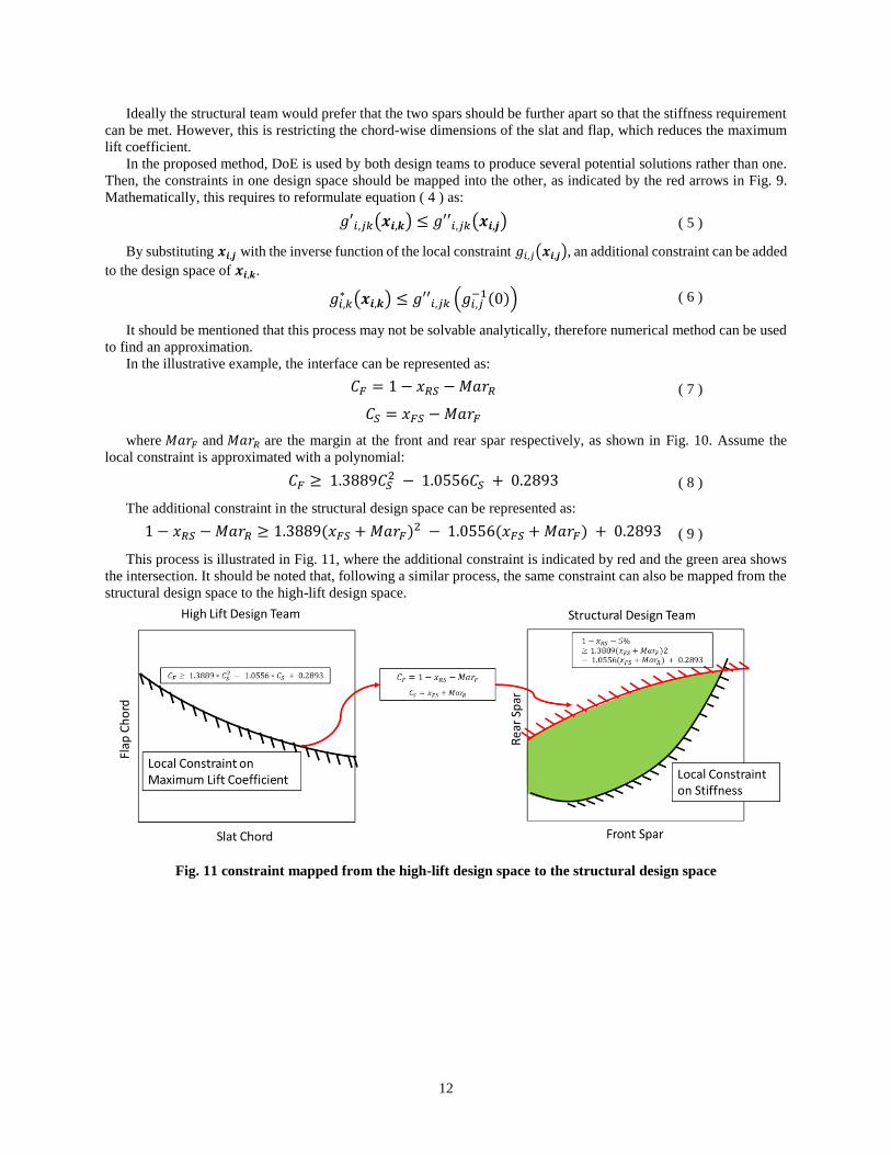
Ideally the structural team would prefer that the two spars should be further apart so that the stiffness requirement

can be met. However, this is restricting the chord-wise dimensions of the slat and flap, which reduces the maximum

lift coefficient.

In the proposed method, DoE is used by both design teams to produce several potential solutions rather than one.

Then, the constraints in one design space should be mapped into the other, as indicated by the red arrows in Fig. 9.

Mathematically, this requires to reformulate equation ( 4 ) as:

𝑔′𝑖,𝑗𝑘(𝒙𝒊,𝒌) ≤ 𝑔′′𝑖,𝑗𝑘(𝒙𝒊,𝒋) ( 5 )

By substituting 𝒙𝒊,𝒋 with the inverse function of the local constraint 𝑔𝑖,𝑗(𝒙𝒊,𝒋), an additional constraint can be added

to the design space of 𝒙𝒊,𝒌.

𝑔𝑖,𝑘∗ (𝒙𝒊,𝒌) ≤ 𝑔′′𝑖,𝑗𝑘 (𝑔𝑖,𝑗

−1(0)) ( 6 )

It should be mentioned that this process may not be solvable analytically, therefore numerical method can be used

to find an approximation.

In the illustrative example, the interface can be represented as:

𝐶𝐹 = 1 − 𝑥𝑅𝑆 −𝑀𝑎𝑟𝑅

𝐶𝑆 = 𝑥𝐹𝑆 −𝑀𝑎𝑟𝐹

( 7 )

where 𝑀𝑎𝑟𝐹 and 𝑀𝑎𝑟𝑅 are the margin at the front and rear spar respectively, as shown in Fig. 10. Assume the

local constraint is approximated with a polynomial:

𝐶𝐹 ≥ 1.3889𝐶𝑆2 − 1.0556𝐶𝑆 + 0.2893 ( 8 )

The additional constraint in the structural design space can be represented as:

1 − 𝑥𝑅𝑆 −𝑀𝑎𝑟𝑅 ≥ 1.3889(𝑥𝐹𝑆 +𝑀𝑎𝑟𝐹)2 − 1.0556(𝑥𝐹𝑆 +𝑀𝑎𝑟𝐹) + 0.2893 ( 9 )

This process is illustrated in Fig. 11, where the additional constraint is indicated by red and the green area shows

the intersection. It should be noted that, following a similar process, the same constraint can also be mapped from the

structural design space to the high-lift design space.

Fig. 11 constraint mapped from the high-lift design space to the structural design space

13

V. Evaluation

In this section, the proposed method is evaluated through a realistic (but not real) aircraft sizing test-case which is

specified in Section V.A. The coordination process is then demonstrated in Section V.B, using an in-house software,

AirCADia [16], [24]. In Section V.C, the proposed method is compared with point-based coordination and feedback

from practicing designers is summarized in section V.D.

A. Test-case Specification

The test-case is organized in three levels, as illustrated in Fig. 12.

Fig. 12 Test-case overview

The first level has a single workflow noted as 𝐹1,1, for selection of wing loading, thrust to weight ratio, and aspect

ratio. The workflow is comprised of constraint analysis, Breguet range equation, and simple algebraic equations to

calculate the actual wing area and thrust. Top Level Requirements (TLRs) are used either as input parameters (e.g.

design range, number of passengers, cruise Mach number and altitude, etc.) or as constraints (e.g. take-off and landing

field length, and climb rate, etc.). In the computation, assumptions are made for aerodynamic coefficients such as

𝐶𝐿𝑚𝑎𝑥, 𝐶𝐷0 , etc. Also assumed are the values for engine thrust lapse rate 𝛼 and specific fuel consumption 𝑆𝐹𝐶 at

different Mach numbers and altitudes.

The second level is separated into airframe and engine, noted as 𝐹2,1 and 𝐹2,2, respectively. In the airframe sizing

problem, a NASA code, FLOPS [19] is used along with some empirical equations from [20]. The task is to define the

basic aircraft geometry (e.g. aspect ratio 𝐴𝑅, wing taper ratio 𝑇𝑅, etc.), given the take-off weight 𝑊𝑇𝑂, reference wing

area 𝑆, and sea level static thrust 𝑇𝑆𝐿 from level 1. In the engine design problem, NPSS [21] is used for analysis. The

task is to match the thrust requirements and specific fuel consumptions at different conditions. These requirements

correspond to the, 𝑆𝐹𝐶, and 𝜶 from level 1.

The third decomposition level concerns the airframe. It consists of the design of high-lift devices 𝐹3,1 and structural

layout 𝐹3,2, respectively, given the wing geometry from level 2. Other (airframe/wing) systems are not considered in

this demonstration for simplicity. The design variables of the high lift system include the chord length of the slat and

flap as illustrated in Fig. 10. ESDU [22] models are used to obtain the whole wing’s maximum lift coefficient (with

high-lift device deployed) which should be no less than the value assumed in level 1. The structural design focuses on

14

the front and rear spar location, using a medium-order model, NeoCASS [23]. A constraint is set on the displacement

of the wing tip. In this level, minimizing the weights of the high-lift devices and structure (wing box) are considered

as objectives.

B. Demonstration of the Proposed Framework

In this section, the proposed methodology is demonstrated through the test-case presented in the previous section.

A design of experiment (DoE) study is conducted to populate the design spaces in each sub-problem, using the in-

house software, AirCADia [16], [24]. Within the same environment, results are visualized and interactive trade-off

studies are conducted to coordinate the assumptions (vertically) and interfaces (horizontally). The expected outcomes

are sets of feasible solutions at each level which will comply with all the constraints, while maintaining promising

performance.

The setup of DoE at the top level is summarized in Table 1.

Table 1 DoE setup at level 1

Category Variables Value/Range Levels

Design Variable 𝑊𝑇𝑂/𝑆 [500, 700] 𝑘𝑔/𝑚2 6

𝑇𝑆𝐿/𝑊𝑇𝑂 [0.25, 0.40] 6

Parameter ℎ𝐶𝑟𝑢𝑖𝑠𝑒 11278 𝑚 (37000 𝑓𝑡) N/A

𝑅𝑑𝑒𝑠 5556 𝑘𝑚 (3000 𝑛.𝑚)

𝑁𝑃𝑎𝑥 160

Assumption 𝐴𝑅 [8.5, 9.5] 3

𝛼𝐶𝑟 [0.18, 0.22] 3

𝐶𝐿𝑚𝑎𝑥𝐿𝐷 [2.8, 3.2] 3

𝑊𝐸/𝑊𝑇𝑂 [0.50, 0.52] 3

𝑆𝐹𝐶 [17, 19] 𝑔/(𝑘𝑁 ∙ 𝑠) 3

Constraint 𝑇𝑂𝐹𝐿 ≤ 2200𝑚 N/A

𝐿𝐹𝐿 ≤ 1900𝑚

𝑀𝑎𝑐ℎ𝐶𝑟 ≥ 0.78 (Maximum 0.82)

ℎ𝐶𝑒𝑖𝑙𝑖𝑛𝑔 ≥ 11887𝑚(39000𝑓𝑡)

𝑅𝐶𝑙𝑖𝑚𝑏 ≥ 1.524𝑚/𝑠(300𝑓𝑡/𝑚𝑖𝑛) One Engine Inoperative During Take-off

The results are shown in Fig. 13 as contour plots, where the green points are the DoE samples and the solid lines

are the constraints. The infeasible regions in each design space are indicated by red areas. As explained in Section

IV.A, the positions of the constraints are dependent on the values of the assumption variables. For Instance, three

different feasible design spaces are shown in Fig. 13 (a), (b), and (c), which are corresponding to (not exclusively)

one pessimistic, one nominal, and one optimistic assumption setting, respectively. In AirCADia, the designer can

specify arbitrary combination of the assumption values in Table 1 and the contour plots will be updated without any

additional model evaluation.

15

Fig. 13 Contour plot of DoE at level 1

The blue points in each design space are representative design solutions of interest in this specific case-study. As

a result, the designer may want to keep a reduced set of 𝑊𝑇𝑂/𝑆 and 𝑇𝑆𝐿/𝑊𝑇𝑂 for further analysis. Then the Breguet

range equation is used for estimation of the take-off weight 𝑊𝑇𝑂. It should be noted that since the assumption variables:

𝑊𝐸/𝑊𝑇𝑂 and 𝑆𝐹𝐶 are specified as intervals, the resulting values of takeoff weight will become a set as well. By

applying the following equations, a set of actual wing areas and sea level static thrusts will be produced and passed

down to the next level:

𝑆 = 𝑊𝑇𝑂/(

𝑊𝑇𝑂

𝑆)

𝑇𝑆𝐿 = 𝑊𝑇𝑂( 𝑇𝑆𝐿𝑊𝑇𝑂

)/𝑛𝐸𝑛𝑔

( 10 )

As mentioned earlier, the second level is divided into airframe and engine design problems, respectively, which in

practice, could be conducted collaboratively by different industrial partners.

In this demonstration, the airframe design involves specification of the aircraft geometry and scaling of a baseline

(rubberized) engine. The scaling factors 𝑘𝑀𝑇𝑂 , 𝑘𝑀𝐶𝐿 , and 𝑘𝑀𝐶𝑅 are corresponding to the baseline engine’s power

rating code: Maximum Take-Off, Maximum CLimb, and Maximum CRuise. Specifically, the upper and lower bounds

of 𝑘𝑀𝑇𝑂 is based on the set of 𝑇𝑆𝐿 from the first level, while the bounds of 𝑘𝑀𝐶𝐿 and 𝑘𝑀𝐶𝑅 are defined such that in the

baseline engine the lower rating thrusts will not exceed the higher ones (e.g. 𝑀𝑇𝑂 ≥ 𝑀𝐶𝐿 > 𝑀𝐶𝑅). The constraints

on range and landing filed length are kept as the same from the first level, while the cruise Mach and service ceiling

are now fixed as inputs for the FLOPS model. The constraint on take-off field length is reduced to 1900 m as it is

identified that most designs in this level are able to meet the original constraint (𝑇𝑂𝐹𝐿 ≤ 2200𝑚) from the first level.

Two new constraints are added on the Time to Climb (𝑇𝑇𝐶) and Approaching Velocity (𝑉𝐴𝑝𝑝). The feasible solutions

will produce the thrust requirements for End of Run way (𝑇𝐸𝑂𝑅), Top of Climb (𝑇𝑇𝑂𝐶), and Mid-CRuise (𝑇𝑀𝐶𝑅). These

requirements are then passed to the engine design team as constraints, where the actual thrusts are produced separately

as output engine performances. Therefore these are considered as the target and responses variables (see also Section

III.A and Section IV.B) between the two teams. It should be noted that the thrust requirements are different from the

power ratings mentioned above.

For the purpose of design coordination, if a set/range of thrust requirements were produced by the airframe design

team (rather than fixed values), then the engine team would have more design freedom, that is, the constraints will

become more flexible. It should be noted that at the top level, assumptions have already been made on the engine

thrust lapse ratio 𝛼 at different flight segments. The thrust requirements from the airframe team (𝑇𝐸𝑂𝑅, 𝑇𝑇𝑂𝐶 , and

𝑇𝑀𝐶𝑅) are actually equivalent to these𝛼’s and can be regarded as an revision of the latter. In addition, the specific fuel

consumption from the top level is formulated as another constraint for engine design. The DoE setups at level 2 for

the airframe and engine designs are shown in Table 2 and Table 3, respectively.

16

Table 2 DoE setup at level 2 for airframe design

Category Variables Value/Range Levels

Design Variable 𝑊𝑇𝑂 [72000, 75000]𝑘𝑔 5

𝑆 [120, 130] 𝑚2 5

𝐴𝑅 [9, 10] 3

𝑇𝑅 [0.24, 0.27] 3

𝑘𝑀𝑇𝑂 [0.88, 1.12] 5

𝑘𝑀𝐶𝐿 [0.97, 1.17] 5

𝑘𝑀𝐶𝑅 [0.9, 1.03] 5

Parameter ℎ𝐶𝑟𝑢𝑖𝑠𝑒 11278 𝑚 (37000 𝑓𝑡) N/A

𝛬0.25 25 degree

𝑁𝑃𝑎𝑥 160

𝑀𝑎𝑐ℎ𝐶𝑟 0.78

Constraint 𝑇𝑂𝐹𝐿 ≤ 1900𝑚 N/A

𝐿𝐹𝐿 ≤ 1900𝑚

𝑅𝐷𝑒𝑠 ≥ 3000𝑛𝑚

𝑉𝐴𝑝𝑝 ≤ 133𝑘𝑡𝑠

𝑇𝑇𝐶 ≤ 26𝑚𝑖𝑛

Table 3 DoE setup at level 2 for engine design

Category Variables Value/Range Levels

Design Variable 𝑊𝑖𝑛𝑇𝑂𝐶 [136, 181]𝑘𝑔/𝑠 4

𝑇𝐷𝑃 [26.7, 31.1]𝑘𝑁 4

𝐵𝑃𝑅 [5.5, 6.5] 3

𝐹𝑃𝑅 [1.6, 1.7] 3

𝐶𝑃𝑅𝐿 [3.0, 3.2] 2

𝐶𝑃𝑅𝐻 [10, 11] 2

Parameter ℎ𝐶𝑟𝑢𝑖𝑠𝑒 11278 𝑚 (35000 𝑓𝑡) N/A

𝑀𝑎𝑐ℎ𝐶𝑟 0.82

Constraint 𝑇𝐸𝑂𝑅 ≥ 𝑇𝐸𝑂𝑅∗ ∈ [95, 107] 𝑘𝑁 N/A

𝑇𝑇𝑂𝐶 ≥ 𝑇𝑇𝑂𝐶∗ ∈ [23, 32]𝑘𝑁

𝑇𝑀𝐶𝑅 ≥ 𝑇𝑀𝐶𝑅∗ ∈ [18.7, 19.4]𝑘𝑁

𝑆𝐹𝐶 ≤ 𝑆𝐹𝐶∗, 𝑆𝐹𝐶∗ ∈ [17, 19]𝑔/(𝑘𝑁 ∙ 𝑠)

The results of airframe design are shown in Fig. 14. As the design space is high-dimensional, multiple contour

plots can be used to visualize the feasible regions. Here two examples are shown in Fig. 14 (a) and (b), which represent

the feasible design space for take-off weight, wing area, aspect ratio, and taper ratio. The resulting thrust requirements

are shown in Fig. 14 (c) and (d), where green colour indicates feasible while red indicates infeasible. The End of

Runway thrusts are clustered in five levels because it’s mainly influenced by the scaling factor 𝑘𝑀𝑇𝑂 (which has 5

levels in the DOE), while the Top of Climb and Mid Cruise thrusts are also influenced by the airframe geometry

parameters, therefore more evenly distributed. The upper and lower bounds of each thrust requirement are represented

by the blue intervals on each axis, obtained as projections of the envelopes containing all the feasible points. These

intervals are [95, 107], [23, 32], and [18.7, 19.4], for 𝑇𝐸𝑂𝑅 , 𝑇𝑇𝑂𝐶 , and 𝑇𝑀𝐶𝑅 , respectively. As discussed earlier, they

are then be passed to the engine design team as flexible constraints as listed in Table 3. A parallel coordinates plot of

all the variable is shown in Fig. 15.

17

Fig. 14 DoE results of airframe design at level 2

Fig. 15 DoE results of airframe design at level 2 in parallel coordinate plot

The results of engine design are shown in Fig. 16 (a) and (b), representing two extreme cases with the least and

most stringent constraint setups, respectively. In Fig. 16 (a), all the thrust requirements are set to their lower bounds,

while the SFC constraint is at its upper limit (refer to Table 3). It can be seen that the end of runway thrust is the active

constraint in this case. In Fig. 16 (b), all the constraint values are set to the other end, except the top of climb thrust,

because among all the engines produced in the DOE study, the highest 𝑇𝑇𝑂𝐶 is 27.2 kN while the original upper limit

is 32 kN. In this case, the SFC becomes an active constraint. Although the design space has been substantially reduced,

there are still enough feasible solutions.

18

Fig. 16 DoE results of engine design at level 2

In practice, the designer can interactively explore the values of constraints by selecting an arbitrary feasible

airframe (with a combination of the engine scaling factors), and use the resulting 𝑇𝐸𝑂𝑅, 𝑇𝑇𝑂𝐶 , and 𝑇𝑀𝐶𝑅 requirements

as constraints for the engine down selection. This process is illustrated in Fig. 17, where the solid and dashed circles

indicate two different airframes (respectively in Fig. 17 (a)) and their corresponding thrust requirements (respectively

in Fig. 17(b)). The different feasible design spaces for the engine team are shown in Fig. 17 (c) and Fig. 17 (d),

respectively.

Fig. 17 Design Coordination between engine and airframe

19

The third level is divided into structural and high-lift design. For a given wing geometry, the layout of spars and

movables (flaps and slats) have to be specified, considering not only their local requirements (regarding strength and

aerodynamics), but also the spatial relationship between them. The DoE setups are summarized in Table 4 and Table

5, respectively.

Table 4 DoE setup at level 3 for structural design

Category Variables Value/Range Levels

Design Variable 𝑥𝐹𝑅 [0.2, 0.4] 6

𝑥𝑅𝑆 [0.6, 0.8] 6

Parameter 𝑆 124 𝑚2 N/A

𝐴𝑅 9.5

𝑇𝑅 0.27

Λ0.25 25 𝑑𝑒𝑔𝑟𝑒𝑒

Constraint 𝑑𝑡𝑖𝑝 ≤ 1𝑚 N/A

𝑊𝑊𝑖𝑛𝑔𝑠𝑡𝑟 ≤ 5000𝑘𝑔

𝜎𝑊𝑚𝑎𝑥 ≤ 140𝑀𝑃𝑎

Table 5 DoE setup at level 2 for high-lift design

Category Variables Value/Range Levels

Design Variable 𝑐𝐹 [0.25, 0.35] 5

𝑐𝑆 [0.1, 0.15] 5

∆𝑐𝐹 [0.02, 0.08] 4

∆𝑐𝑆 [0.02, 0.08] 4

Parameter 𝑆 124 𝑚2 N/A

𝐴𝑅 9.5

𝑇𝑅 0.27

Λ0.25 25 𝑑𝑒𝑔𝑟𝑒𝑒

Constraint 𝐶𝐿𝑚𝑎𝑥𝐿𝐷 ≥ 𝐶𝐿𝑚𝑎𝑥𝐿𝐷

∗ , 𝐶𝐿𝑚𝑎𝑥𝐿𝐷

∗ ∈ [2.8, 3.2] N/A

The result of the structural DOE is shown in Fig. 18, where (a) is the design space of the front and rear spar location,

and (b) is the PCP of all the variables. It can be seen that the output results are highly non-linear. However in general,

the feasible region is situated in the bottom left part of the design space, which means that in this case it is beneficial

to put both spars close to the leading edge.

Fig. 18 DoE results of structural design at level 3

The results of the high-lift DOE is shown in Fig. 19 where (a) and (b) are the contour plots of different 2D projections

of the high-dimensional design space. This is as expected, because larger flap and slat sizes will lead to higher values

for 𝐶𝐿𝑚𝑎𝑥𝐿𝐷.

20

Fig. 19 DoE results of high-lift design at level 3

As explained in Section IV.B, there is an interface between the structure and high-lift devices (see Fig. 10 and equation

( 7 )). Because there are no shared variables between the structural and high-lift design team, the constraints in one

design space need to be mapped into the other for design coordination. In this case, as the structural design space is

highly non-linear, it is more convenient to convert the constraints for high-lift devices.

From Fig. 19 (a), the following relationships can be obtained with approximation:

𝐶𝑆 ≥ 5.71𝐶𝐹2 − 4.54𝐶𝐹 + 0.95 ( 11 )

Substituting equation ( 7 ) in equation ( 11 ), an additional constraints for the structural design is defined:

𝑥𝐹𝑆 −𝑀𝑎𝑟𝐹 ≥ 5.71(1 − 𝑥𝑅𝑆 −𝑀𝑎𝑟𝑅)2 − 4.54(1 − 𝑥𝑅𝑆

−𝑀𝑎𝑟𝑅) + 0.95 ( 12 )

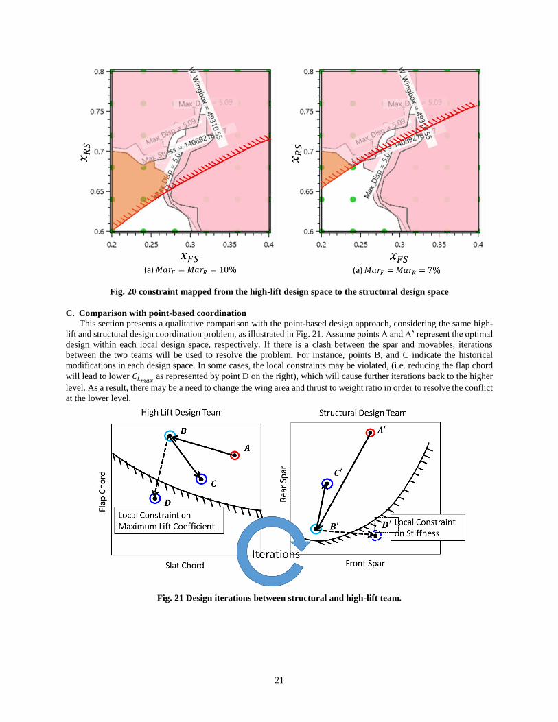
The red lines in Fig. 20 are the additional constraints mapped from the high-lift design space into the structural design

space, and the while areas are the feasible regions for both high-lift and structural design teams. Based on the values

of the margins (𝑀𝑎𝑟𝐹 and 𝑀𝑎𝑟𝑅), the position of the constraint will be different as illustrated by Fig. 20 (a) and (b).

21

Fig. 20 constraint mapped from the high-lift design space to the structural design space

C. Comparison with point-based coordination

This section presents a qualitative comparison with the point-based design approach, considering the same high-

lift and structural design coordination problem, as illustrated in Fig. 21. Assume points A and A’ represent the optimal

design within each local design space, respectively. If there is a clash between the spar and movables, iterations

between the two teams will be used to resolve the problem. For instance, points B, and C indicate the historical

modifications in each design space. In some cases, the local constraints may be violated, (i.e. reducing the flap chord

will lead to lower 𝐶𝐿𝑚𝑎𝑥 as represented by point D on the right), which will cause further iterations back to the higher

level. As a result, there may be a need to change the wing area and thrust to weight ratio in order to resolve the conflict

at the lower level.

Fig. 21 Design iterations between structural and high-lift team.

22

VI. Conclusions

Presented in this paper is a framework for the design coordination of hierarchical (multi-level) collaborative design

studies. The need for solving such problems arose from interaction with the industrial partners in the APROCONE

project.

By employing margin management and set-based design principles and methods, the proposed framework enables

coordination and conflict resolution between design teams within and/or across different product (design)

decomposition levels. Two strategies for handling vertical and horizontal design coordination are proposed. The

former is based on flexible margins/targets while the latter is handled by intersecting feasible design spaces of the

collaborating teams.

An industrially relevant test-case, similar to the one presented here was used to demonstrate the proposed

framework to the APROCONE consortium. The usefulness of the proposed approach was largely confirmed by

practicing engineers and architects from the industrial partners.

Future work includes:

1) Further generalization of the framework, especially regarding the horizontal integration. This requires

advancing the technique to map constraints across different domains analytically or numerically. This will

also be useful for extracting design rules so that knowledge can be reused in future products.

2) Development of a method to handle models with evolving fidelity. For instance, by updating the results from

lower-order models with higher-order ones as more details become available.

3) Reduce the computational cost, by using more efficient sampling strategies and surrogate modelling

techniques.

4) Development of probabilistic metrics for quantitative evaluation of the approach. This involves estimates for

potential nugatory iterations in both point-based and set-based approaches.

Acknowledgments

The research leading to these results has received funding from the Aerospace Technology Institute (ATI) in the UK,

under the Advanced Product Concept Analysis Environment (APROCONE) project (Ref no. 113092).

References

[1] M. M. Andreasen, A. H. B. Duffy, K. J. MacCallum, J. Bowen, and T. Storm, “The Design Co-ordination

Framework: key elements for effective product development,” in 1st Int. Engineering Design Debate, 1996,

pp. 151–172.

[2] A. H. B. Duffy, M. M. Andreasen, K. J. MacCallumx, and L. N. Reijers, “Design Coordination for Concurrent

Engineering,” J. Eng. Des., 1993.

[3] S. C.-Y. Lu, J. Cai, W. Burkett, and F. Udwadia, “A Methodology for Collaborative Design Process and

Conflict Analysis,” CIRP Ann., 2007.

[4] K. S. Trivedi, A. Bobbio, J. Muppala, K. S. Trivedi, A. Bobbio, and J. Muppala, “Fixed-Point Iteration,” in

Reliability and Availability Engineering, 2017.

[5] M. Tichem, “Designer support for product structuring--development of a DFX tool within the design

coordination framework,” Comput. Ind., 1997.

[6] T. Zang and L. Green, “Multidisciplinary design optimization techniques - Implications and opportunities for

fluid dynamics research,” 2013.

[7] E. J. Cramer, J. E. Dennis, Jr., P. D. Frank, R. M. Lewis, and G. R. Shubin, “Problem Formulation for

Multidisciplinary Optimization,” SIAM J. Optim., 2005.

[8] J. Sobieszczanski-Sobieski, “Optimization by decomposition: A Step from Hierarchic to Non- Hierarchic

systems.,” Nasa Tech. Memo., 1988.

[9] J. Sobieszczanski-Sobieski, T. D. Altus, M. Phillips, and R. Sandusky, “Bilevel Integrated System Synthesis,”

AIAA J., 2000.

[10] R. D. Braun, “Collaborative optimization: An architecture for large-scale distributed design,” 1996.

[11] H. M. Kim, N. F. Michelena, P. Y. Papalambros, and T. Jiang, “Target Cascading in Optimal System Design,”

J. Mech. Des., 2003.

[12] J. R. R. A. Martins and A. B. Lambe, “Multidisciplinary Design Optimization: A Survey of Architectures,”

AIAA J., 2013.

[13] H. M. Kim, D. G. Rideout, P. Y. Papalambros, and J. L. Stein, “Analytical Target Cascading in Automotive

Vehicle Design,” J. Mech. Des., 2003.

[14] D. K. Sobek, A. Ward, and J. Liker, “Toyota’s principles of set-based concurrent engineering,” Sloan Manage.

23

Rev., 1999.

[15] A. Riaz, M. D. Guenov, and A. Molina-Cristóbal, “Set-Based Approach to Passenger Aircraft Family Design,”

J. Aircr., vol. 54, no. 1, pp. 310–326, Jan. 2017.

[16] M. D. Guenov, M. Nunez, A. Molina-Cristóbal, V. Datta, and A. Riaz, “Aircadia – an Interactive Tool for the

Composition and Exploration of Aircraft Computational Studies At Early Design Stage,” 29th Congr. Int.

Counc. Aeronaut. Sci., 2014.

[17] L. K. Balachandran and M. D. Guenov, “Computational Workflow Management for Conceptual Design of

Complex Systems,” J. Aircr., vol. 47, no. 2, pp. 699–703, Mar. 2010.

[18] Y. Bile, A. Riaz, M. D. Guenov, and A. Molina-Cristobal, “Towards Automating the Sizing Process in

Conceptual (Airframe) Systems Architecting,” in AIAA/ASCE/AHS/ASC Structures, Structural Dynamics, and

Materials, 2018.

[19] L. A. Mccullers, “Aircraft configuration optimization including optimized flight profiles,” in Symposium on

Recent Experiences in Multidisciplinary Analysis and Optimization, 1984.

[20] D. P. Raymer, Aircraft design : a conceptual approach, 5th edn. Reston: American Institute of Aeronautics

and Astronautics, 2012.

[21] J. K. Lytle, “The Numerical Propulsion System Simulation: An Overview,” 2000.

[22] “ESDU 99031 Computer program for estimation of lift curve to maximum lift for wing-fuselage combinations

with high-lift devices at low speeds.”

[23] L. Cavagna, S. Ricci, and L. Riccobene, “A Fast Tool for Structural Sizing, Aeroelastic Analysis and

Optimization in Aircraft Conceptual Design,” in 50th AIAA/ASME/ASCE/AHS/ASC Structures, Structural

Dynamics, and Materials Conference, 2009.

[24] M. D. Guenov, M. Nunez, A. Molina-Cristóbal, V. Sripawadkul, V. C. Datta, and A. Riaz, “Composition,

Management, and Exploration of Computational Studies at Early Design Stage,” in Computational

Intelligence in Aerospace Sciences, Progress in Astronautics and Aeronautics, M. Vasile and V. M. Becerra,

Eds. Reston: American Institute of Aeronautics and Astronautics, 2014, pp. 415–460.