a sequential pattern mining approach to design taxonomies
TRANSCRIPT

THEORETICAL ADVANCES
A sequential pattern mining approach to design taxonomiesfor hierarchical music genre recognition
Sylvain Iloga1,2,3• Olivier Romain2
• Maurice Tchuente3
Received: 31 December 2015 / Accepted: 8 September 2016
� Springer-Verlag London 2016
Abstract In this paper, music genre taxonomies are used
to design hierarchical classifiers that perform better than
flat classifiers. More precisely, a novel method based on
sequential pattern mining techniques is proposed for the
extraction of relevant characteristics that enable to propose
a vector representation of music genres. From this repre-
sentation, the agglomerative hierarchical clustering algo-
rithm is used to produce music genre taxonomies.
Experiments are realized on the GTZAN dataset for per-
formances evaluation. A second evaluation on GTZAN
augmented by Afro genres has been made. The results
show that the hierarchical classifiers obtained with the
proposed taxonomies reach accuracies of 91.6 % (more
than 7 % higher than the performances of the existing
hierarchical classifiers).
Keywords Audio processing � Automatic taxonomy
generation � Music genre recognition � Hierarchicalclassification � Sequential pattern mining � Histogrammining
1 Introduction
Nowadays, broadcast radio is a source of multimedia
content under-exploited. Digital radio stations broadcast
meta-data (traffic, music cover, meteorological data, radio
name, etc.), and, by using the RDS norm, FM analogue
bands deliver various information. These meta-data enrich
not only the diversity of available broadcast content, but
also the possibilities of indexing this content, either using
the contained meta-data, or via original features extracted
from the radio signal themselves. It is necessary to develop
new search engines that enable the internet user to navigate
efficiently through these multimedia streams produced by
radio broadcast. The use of audio indexing techniques in
the broadcast media market will also be critical for radio on
demand applications. These technologies will provide new
services such as criterion-based programming (genre- or
artist- specific, publicity filtering, etc.). The two main
issues in such applications are the simultaneous demodu-
lation of entire broadcast bands and the music genre clas-
sification. While the first issue has been solved [1], the
second one remains pending.
The extraction of some information from music samples
is currently the subject of many studies. To improve the
efficiency of recognition systems, several authors have
proposed hierarchical approaches. The main idea is that a
classifier applied at an inner node of the taxonomy allows
solving a classification problem with a small number of
classes. Therefore, these approaches are more efficient than
flat multi-class classifiers [2].
Several taxonomies have been designed to perform
hierarchical classification in various domains. A detailed
review of performance evaluation based on taxonomies can
be found in [3]. The 3 following motivations for the use of
taxonomies in music genres classification are stated in [4]:
& Sylvain Iloga
Olivier Romain
Maurice Tchuente
1 Higher Teachers’ Training College, Department of Computer
Science, University of Maroua, P.O. Box 55, Maroua,
Cameroon
2 Laboratoire ETIS, UMR 8051, Universite de Cergy-Pontoise,
CNRS, ENSEA, av du ponceau, 95000 Cergy-Pontoise,
France
3 IRD UMI 209 UMMISCO and LIRIMA, University of
Yaounde 1, P.O. Box 337, Yaounde, Cameroon
123
Pattern Anal Applic
DOI 10.1007/s10044-016-0582-7
1. Taxonomies improve usability and search success rate.
2. A hierarchy enables to identify the existing links of
dependence between the genres.
3. Hierarchical classifiers based on taxonomies implement
the divide-and-conquer principle that makes the errors
concentrate within the given level of the hierarchy.
In music genre recognition, most of the existing tax-
onomies are human-generated [2, 4–6]. Other
authors [7, 8] proposed techniques to automatically gen-
erate taxonomies. However, in some of these publica-
tions [4, 6], experiments were not cross-validated, and it is
difficult to compare the real performances of the classifiers.
Additionally the gain in accuracy provided by the existing
methods is generally low. The manually generated tax-
onomies proposed in [2, 4–6] exhibit accuracy gains not
greater than 5.1 %. The same observation is made in [7]
where the proposed automatically generated taxonomies
provide accuracy gains not greater than 2 %. The highest
accuracy gain reached 14.67 % and was obtained by the
automatically generated taxonomy proposed in [8].
In this paper, a new approach to extract taxonomies of
music genres is proposed. It is mainly based on sequential
pattern mining techniques. Given a family G of music genres,
these techniques are used to initially identify relevant sets of
characteristics for each genre of G. These features enable to
propose a vector representation for each genre. The similar-
ities between these vectors are then used as input to the
Agglomerative Hierarchical Clustering (AHC) algorithm [9],
in order to generate a taxonomy. Finally, the generated tax-
onomy is tested in a hierarchical classification process.
The rest of this paper is organized as follows: The state
of the art is presented in Sect. 2, and a detailed description
of the proposed approach is given in Sect. 3. Experimental
results are presented in Sect. 4 and the last section is
devoted to the conclusion.
2 State of the art
2.1 Hierarchical music genres classification
As noted earlier in Sect. 1, some previous work on hierar-
chical music genre classification have relied on human-
generated taxonomies. A classical way to manually design
genre taxonomies consists in gathering the genres according
to some general descriptors such as the feeling (soft, noisy,
etc.), the geographical origin (Afro, Latino, etc.), the music
instruments used (piano, guitar, etc.) and the language
(English, French, etc.). Such manually generated taxonomies
may not match with the natural groups of genres detected
when low-level music descriptors are used [7]. This differ-
ence results from the fact that manually generated hierar-
chies often use human semantics, and therefore are mainly
suitable for human use, while the automatically generated
taxonomies are optimized for computational classifiers [4].
This is why in [10], Pachet analyzed existing taxonomies of
music genres and derived some criteria that should lead the
design of a taxonomy of music genres.
In [2], Brecheisen relied on the manually generated tax-
onomy presented in Fig. 1a to design a hierarchical classifier
for 11 music genres (500 songs, 30 s each) after extracting the
5 following music descriptors: Mel Frequency Cepstral
Coefficients (MFCCs), spectral flux, spectral rolloff, beat
histogram and pitch histogram. He used Support Vector
Machines (SVMs) as classifiers and after a 90–10 % cross-
validation, his hierarchical classifier performed slightly worse
than the flat classifier: This method reached 72.01 % for the
flat classifier and 70.03 % for the hierarchical classifier.
Tao manually generated in [4] the taxonomy presented
in Fig. 1b to realize the hierarchical classification of the 10
genres of GTZAN [11]. After extracting 7 music descrip-
tors, he used SVMs with linear kernels implemented in the
LibSVM library as classifier. No cross-validation was
realized. He performed one single training step including
70 % of the data and one test step including 30 % of the
data. He obtained accuracies of 72 % for the flat classifier
and 72.7 % for the hierarchical classifier. Tao also pro-
posed in [4] an approach to automatically design music
genres taxonomies. The taxonomy was then generated by
applying a hierarchical clustering algorithm. The main
limitation of this method is the fact that the taxonomy
depends on the selected classifier. Indeed, two genres
naturally different may be represented by vectors close to
one another, due to a poor classifier. These automatically
generated taxonomies were not used for hierarchical clas-
sification in that work.
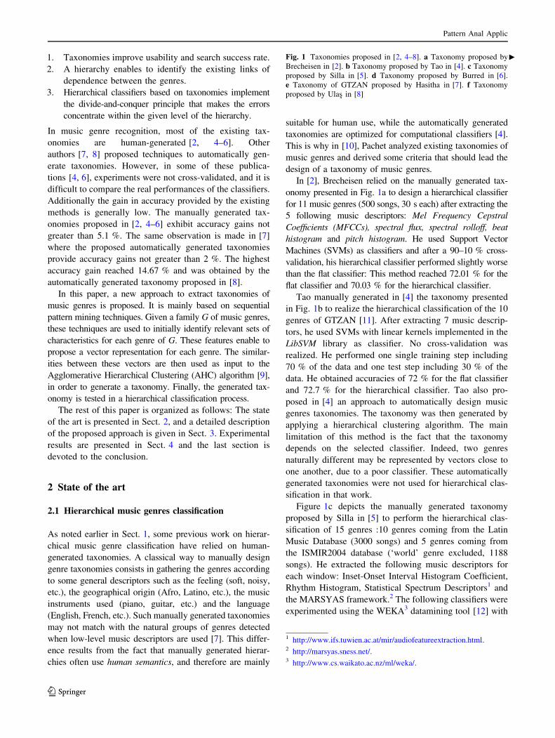
Figure 1c depicts the manually generated taxonomy
proposed by Silla in [5] to perform the hierarchical clas-
sification of 15 genres :10 genres coming from the Latin
Music Database (3000 songs) and 5 genres coming from
the ISMIR2004 database (‘world’ genre excluded, 1188
songs). He extracted the following music descriptors for
each window: Inset-Onset Interval Histogram Coefficient,
Rhythm Histogram, Statistical Spectrum Descriptors1 and
the MARSYAS framework.2 The following classifiers were
experimented using the WEKA3 datamining tool [12] with
cFig. 1 Taxonomies proposed in [2, 4–8]. a Taxonomy proposed by
Brecheisen in [2]. b Taxonomy proposed by Tao in [4]. c Taxonomy
proposed by Silla in [5]. d Taxonomy proposed by Burred in [6].
e Taxonomy of GTZAN proposed by Hasitha in [7]. f Taxonomy
proposed by Ulas in [8]
1 http://www.ifs.tuwien.ac.at/mir/audiofeatureextraction.html.2 http://marsyas.sness.net/.3 http://www.cs.waikato.ac.nz/ml/weka/.
Pattern Anal Applic
123

Pattern Anal Applic
123

default parameters: K-Nearest Neighbors (KNNs), Naive
Bayes (NBs), Multi Layers Perceptrons (MLPs) and SVMs.
After a 80–20 % cross-validation, the best accuracy he
obtained for his hierarchical classification was 78.82 %.
In [6], Burred performed the hierarchical classification of
the 10 genres of the MIREX2005 database (1515 songs, 30 s
each) using themanually generated audio taxonomy shown in
Fig. 1d. He extracted 15music descriptors and used Gaussian
Mixture Models (GMMs) developed into a M2K framework
(using MATLAB integration modules) as classifiers. No
cross-validation was realized. The training and the classifi-
cation phases, respectively, included 66.4 and 33.6 % of the
data. He obtained accuracies of 54.12 and 59.22 %, respec-
tively, for the flat and the hierarchical classifiers.
In [7], Hasitha proposed an approach to automatically
generate music genres taxonomies. He extracted 13 music
descriptors to describe each audio window. Taxonomies
were generated for the two following experimental data-
bases: GTZAN presented in Fig. 1e and HBA (15 genres,
500 songs per genre, 30 s each). The PROjected CLUS-
tering algorithm (PROCLUS) [13] executed in a top-down
manner was used to generate taxonomies. This algorithm
enables the user to control the breadth of the generated
taxonomy by setting the number K of desired clusters. They
selected the K-Mediods method for distance measurement.
The algorithm starts with a single cluster containing all the
genres as input, then the output clusters are used as input
for the next step in a repetitive manner until the generation
of clusters containing only one genre. LibSVM, Sequential
Minimal Optimization (SMO that is SVMs with polyno-
mial kernel), KNNs, Decision Trees (DTs), Logistic
Regression (LOG) and MLPs were combined during the
classification phase. At each node of the hierarchy, he
selected both the best attribute as proposed in [14] and the
suitable classifier to be used. Attribute selection is com-
monly performed by techniques like Principle Component
Analysis (PCA) and Linear Discriminant Analysis (LDA).
Most of the widely used attribute selection techniques in
music genre classification are described in [14]. The hier-
archical classification produced the following results: (1)
On GTZAN, the hierarchical classifier obtained 72.9 %,
while the corresponding flat classifier produced 70.9 %. (2)
On HBA, the hierarchical classifier obtained 78.6 %, while
the corresponding flat classifier produced 77.2 %.
In [8], Ulas used GMMs to model the inter-genre sim-
ilarities in order to automatically generate the taxonomy
presented in Fig. 1f. After the taxonomy generation, these
GMMs were later used to perform hierarchical classifica-
tion. For each audio window, he extracted 7 timbre music
descriptors. Experiments were realized on 9 genres all
coming from the GTZAN database (‘blues’ excluded), but
only 20 songs were considered per genre. To automatically
construct the hierarchy of N genres, he proceeded as
follows:
1. Consider each genre as a cluster of size 1.
2. Train one GMM for each cluster using the songs of all
the genres belonging to the considered cluster
3. Realize the flat classification of the songs of each
cluster considering these models ; this step leads to a
confusion matrix C ¼ fcijg.4. Find the two clusters i� and j� having the highest
confusion value in C and merge them into a new
cluster: ði�; j�Þ ¼ argmax cij with ði 6¼ jÞ5. Repeat steps 2–4 until one single cluster is obtained.
The 90–10 % cross-validation he performed provided
accuracies of 63.33 % for the flat classifier and 78 % for
the hierarchical classifier.
2.2 Sequential patterns in music genres
classification
Many authors have already used sequential pattern mining
techniques to perform music genres classification. Con-
klin [15]modeled themelodyof a songas a sequential pattern.
He extracted a list of association rules for the two classes of his
training database composed of 102Austrian and 93Swiss folk
song melodies. The classification phase was realized by a
decision list method based on these association rules. Lin [16]
extracted Significant Repeating Patterns from the rhythm and
the melody of music excerpts to build training databases. To
realize the classification of a candidate song c, he adopted a
dynamic programming approach to measure the similarities
between c and the content of the various training databases.
In [17, 18], Ren first transformed each music piece into a
sequential pattern composed of hiddenMarkovmodel indices.
The frequent sequential patterns of each genre are then dis-
covered, and their occurrence frequencies are calculated.
Finally, K-NN (in [17]) and SVMs (in [18]) classifiers are
used during the classification phase. The main difference
between these work and the proposed approach relies on the
semantic of the sequential patterns. Table 1 presents the
details of related work on hierarchical music genre classifi-
cation and on flat music genre classification using sequential
pattern mining techniques.
Before describing the methodology of the approach pro-
posed here, basic concepts about sequential patterns and some
sequential pattern mining algorithms are first presented. In the
following, an item is considered as the smallest information
that can be found in a sequential pattern database d. Thus anitem can for example be an integer or a character identifying
an information. Let X ¼ fx1; x2; . . .; xkg be the set of all the
items appearing in d. A subset of X is called an itemset. We
assume here that all the items of an itemset are sorted in a
Pattern Anal Applic
123
given order, such as alphabetic or numeric order. A sequential
pattern s ¼ hs1; s2; . . .; smi is an ordered list of itemsets si �X with i 2 ½1;m�. The number of itemsets of s denoted |s| is
called the size of s. The total number of items in s denoted
l(s) is called the length of s. A sequential pattern a ¼ha1; a2; . . .; ami is a sub-sequence of another sequential pat-
tern b ¼ hb1; b2; . . .; bniðaYbÞ if there exist i1; i2; . . .; imsuch that the two following conditions are verified [19]: (1)
1� i1\i2\ � � �\im � n; (2)
a1 � bi1 ; a2 � bi2 ; . . .; and am � bim . When a is a sub-se-
quence of b, b is called super-sequence of a and it can be saidthat b contains a.
A sequential patterns database d ¼ fs1; s2; . . .; sng is a
set of sequential patterns and jdj is the number of
sequential patterns in d. As described in Eq. 1, the fre-
quency of a sequential pattern a in d denoted freqða; dÞ, isthe number of sequential patterns in d which contain a. Thesupport of a sequential pattern a in d denoted supða; dÞ isobtained by dividing the frequency of a by jdj. Given a
minimum support threshold min sup, a sequential pattern ais frequent if and only if its support is greater than min sup.
More formally, given d and min sup:
freqða; dÞ ¼ jfsjs 2 d and aYsgj
supða; dÞ ¼ freqða; dÞjdj
ða is frequentÞ , ðsupða; dÞ�min supÞ
8>><
>>:
ð1Þ
For instance, let X ¼ f1; 2; . . .; 8g and d ¼ fs1; s2; s3; s4gbe the sequential patterns database of Table 2. Consider
a ¼ hð6Þð27Þi:
1. The super-sequences of a in d are s1; s3 and s4. The
corresponding items are written in bold in the table.
2. freqða; dÞ ¼ jfs1; s3; s4gj ¼ 3 and supða; dÞ ¼ 34
3. for min sup ¼ 0:5, a is frequent. But for
min sup ¼ 0:9, a is not frequent.
The problem of frequent sequential pattern mining can be
specified as follows: given a sequential pattern database d and
a minimum support threshold min sup, one would like to
discover all the frequent sub-sequences of the sequential
patterns of d with respect to min sup. The following algo-
rithms have been developed to perform frequent sequential
pattern mining: Apriori [20], GSP [21], SPADE [22], Free-
span [23] and Prefixspan [19]. Several other algorithms have
been developed and a detailed survey on sequential pattern
mining algorithms can be found in [24].
2.3 Problem statement
As presented in Table 1, the existing hierarchical
approaches [2, 4, 7] show accuracy gains not greater than
2 %. The taxonomies used in [2, 4–6] are generated by
humans and no cross-validation is applied in [4, 6, 7]
Table 1 Performances of the cited work in hierarchical music genres classification and flat music genres classification using sequential patterns
mining techniques
Referenced
work
Number of
genres
Songs per
genre
Taxo. Auto.
Generated
Database Classifiers Cross
valid.
Flat
acc.
Hier.
acc.
Gain
acc.
Year
Brecheisen [2] 11 �30 No Custom SVM Yes 72.01 70.03 -1.98 2006
Tao [4] 10 100 No GTZAN SVM No 72.01 72.69 þ0.68 2005
Silla [5] 15 [52, 615] No ISMIR 2005,
LMD
KNN, MLP, NB,
SVM
Yes – 78.82 – 2009
Burred [6] 10 [100 No MIREX 2005 GMMs No 54.12 59.22 þ5:1 2003
Hasitha [7] 15 500 Yes HBA KNN, DT, LOG, No 77.2 78.6 þ1.4 2012
10 100 (PROCLUS) GTZAN SVM, MLP 70.9 72.9 þ2
Ulas [8] 9 20 Yes (GMMs) GTZAN GMMs Yes 63.33 78 þ14:67 2005
Conklin [15] 2 f93; 102g – Essen Folk
Song
Decision list,
Association rules
Yes 77 – – 2009
Lin [16] 7 – – Custom Dynamic
Programming
No 49.18 – – 2004
Ren [17] 5 [354, 785] – Magnatunes,
Dortmund
KNN No 74.19 – – 2010
Ren [18] 10 100 – GTZAN SVMs Yes 74.5 – – 2011
Bold represents that in these related works: (1) the taxonomies were generated manually, (2) the classification phases were not cross-validated
and (3) the accuracy gains were very low
Table 2 Database dNo. Content
s1 hð23Þð167Þð3Þð267Þð24Þis2 hð15Þð169Þð4Þis3 hð56Þð2478Þð37Þis4 hð168Þð2357Þi
Pattern Anal Applic
123

during the classification step. This is a drawback because a
classifier may generate good classification results for par-
ticular training and test sets of the considered database,
and exhibit poor classification accuracy after cross-vali-
dation. On the other hand, the automatic generation of
taxonomies is useful for huge music databases that are
difficult or even impossible to handle manually. Another
advantage of automatic generation is that a priori knowl-
edge or particular expertise on the genres is not required.
The natural clusters existing in the database are automati-
cally detected according to the selected low-level music
descriptors. Nevertheless, the experts’ contributions may
be essential to validate the resulting taxonomy.
This paper aims at providing better classification per-
formances than existing work by proposing an automatic
approach for taxonomy generation. Sequential pattern
mining techniques are applied to propose new vectorial
music genres descriptors. These vectors are later used as
input for a hierarchical clustering algorithm to generate the
taxonomy. Cross-validation is applied during the classifi-
cation step. Several commonly used classifiers are used to
illustrate the performance gains obtained with the corre-
sponding hierarchical classifiers.
3 The proposed approach
3.1 Main idea
The main idea of this work is based on a fundamental
observation about both music samples and genres. When
listening to some music excerpts, one has the impression of
shifting from one genre to another. This happens when the
corresponding genres have strong similarities. For exam-
ple, a song may seem to belong to reggae at its beginning,
but transits to country for a while before shifting to blues.
Let G ¼ fg1; g2; . . .; gNg be a family of genres and let c be
a song. The previous remark allows to see c as a sequence
of genres of G, each term of the sequence corresponding to
a short time interval. In some cases, it is even difficult to
assign a particular genre to a short time interval of a music
excerpt because it has some characteristics that can be
found in several genres. Therefore, the notation presented
in Eq. 2 is adopted for a song where ðgj1gj2. . .gjkjÞ is the setof the possible genres corresponding to the time interval of
index j. Such an expression is called a sequential pattern
i.e., a sequence of subsets of genres’ labels.
c ¼ ðg11. . .g1k1Þðg21. . .g2k2Þ. . .ðgw1. . .gwkwÞ ð2Þ
3.2 Methodology
To perform hierarchical classification, the methodology
presented in Fig. 2 and proposed in this paper proceeds in
10 steps grouped in the 6 following phases: Music
descriptors extraction (steps 1–3), transformation into
sequential patterns (steps 4–5), characteristic sequential
patterns extraction (steps 6–7), computation of vector
descriptors for genres (step 8), hierarchical clustering (step
9) and hierarchical classification (step 10). Details about
each step are presented below:
1. Choose the time interval.
2. Choose the features that will be used.
3. Represent each training song c as a sequence c ¼v1v2. . .vw of vectors of descriptors.
4. For each genre gi, apply a clustering algorithm on the
collection of vectors of descriptors corresponding to
its training songs to obtain k central vectors per genre.
5. Transform each representation c ¼ v1v2. . .vw into a
sequential pattern as indicated by Eq. 2 where
Fig. 2 Methodology of the proposed approach
Pattern Anal Applic
123

ðgj1gj2. . .gjkjÞ is the set of genres associated with the
nearest central vectors of vj. This generates a
database di of sequential patterns for each genre gi.
6. Apply a sequential pattern mining algorithm on di tocompute the set ri of frequent patterns of each genre
gi.
7. Extract from ri the set ui of characteristics frequent
patterns corresponding to gi.
8. Use all the uið1� i�NÞ to compute the vector
descriptor Ui�!
of genre gi for i ¼ 1; . . .;N. Ui�!
is a
positive N-dimensional real vector with normalized
components.
9. Build the taxonomy based on the vector descrip-
tors computed at step 8 by applying a hierarchical
clustering algorithm.
10. Perform the hierarchical classification based on the
computed taxonomy using an efficient flat classifier.
3.3 Music descriptors extraction
The time interval of the first step of the methodology is
set at one second. Therefore, music features were
extracted from music excerpts within texture windows of
one second as it was done in [25]. In a survey proposed
in 2010, Mitrovic drew a list of 70 highly utilized audio
descriptors based on 200 publications [26]. For steps 2
and 3 of the methodology, timbre music descriptors have
been adopted to generate a taxonomy. The following
wide-spread short term timbre music descriptors to gen-
erate the taxonomy are extracted: Mel Frequency Cep-
stral Coefficients (MFCCs), Spectral centroid, Spectral
rolloff, Spectral flux and Zero crossing rate. Details about
the extraction of these music descriptors can be found
in [25].
After the taxonomy generation, some rhythm music
descriptors were extracted and combined with the previous
timbre music descriptors during the classification step. The
4 following rhythm music descriptors were extracted: bpm
peak values (1), Rhythm Patterns (200), Rhythm Histogram
(60) and Statistical Spectrum Descriptor (140). These
rhythm music descriptors have been selected because they
provided an accuracy of 74.9 % when Lidy made the flat
classification of GTZAN in [27]. They were extracted
using the online available MATLAB framework [28]
developed by Lidy. The selected rhythm music descriptors
were not used for the taxonomy generation because they
required a considerable amount of data (more than one
second) to produce reliable results.
3.4 Transformation of a song into a sequential
pattern
As shown in Fig. 3, the global transformation process
includes a training step. During the training of each genre
of the family G, the collection of vectors of music
descriptors (one per second) coming from all its training
excerpts was taken into account. The k-means method was
first applied to cluster the collection of vectors into k clus-
ters. This produces k central vectors per music genre as
stated in the 4th step of the methodology. After the training
step, the K-NN algorithm has been applied to perform the
transformation as specified in step 5 of the methodology.
3.4.1 Transformation with the NN algorithm
Let us first present the simple case of the K-NN algorithm
with K ¼ 1. To obtain the sequential pattern of a music
excerpt c, its sequence of vectors of music descriptors is
first extracted. This produces c ¼ v1v2. . .vw. For each
Fig. 3 Transformation of a song into a sequential pattern
Pattern Anal Applic
123

vector vj of c, the Nearest Neighbor algorithm is applied to
determine its nearest central vector among all the central
vectors of the N genres. Then vj is replaced by the genre
associated with this central vector. Therefore, c is trans-
formed into the sequential pattern hðgi1Þðgi2Þ. . .ðgiwÞi. Aspresented in Fig. 4, the resulting representation adheres
with the one of Eq. 2.
Consider the song c of Fig. 4 represented as a sequence
of 5 vectors. If squares, circles and triangles represent
respectively the central vectors of genres classical, jazz
and blues then the corresponding sequential pattern is c =
h(jazz) (blues) (classical) (blues) (classical) i. This means
that the first second of c contain characteristics of jazz, the
next second contains those of blues, and so on. When this
principle is applied to all the training excerpts of each
genre gi, it outputs one training sequential patterns data-
base di.
3.4.2 First transformation with the K-NN algorithm
With the NN algorithm, one single central vector is con-
sidered to determine the genre gij associated with a vector
vj of a song c. But an information is still unexploited
because in the neighborhood of vj, there may exist several
other central vectors associated with other genres. To avoid
this situation, the K-NN algorithm with ðK[ 1Þ is applied.We thus determine the set of all the genres associated with
the K nearest central vectors of vj. Then vj is replaced by
this set of genres which becomes an itemset that may
contain more than one genre. c is then transformed into the
sequential pattern hsi1 ; si2 ; . . .; siwi where every sij is a set of
genres as shown in Fig. 5.
When the 4-NN algorithm is applied in Fig. 5 in similar
conditions as those of Fig. 4, the song c is transformed into
the sequential pattern c = h(classical jazz) (blues) (classicaljazz) (classical jazz blues) (classical blues) i. This means
that the first second of c contains characteristics of clas-
sical and jazz, the next second contains characteristics of
blues, and so on. This principle is applied to all the training
songs of each genre gi of G to obtain one training
sequential patterns database di.
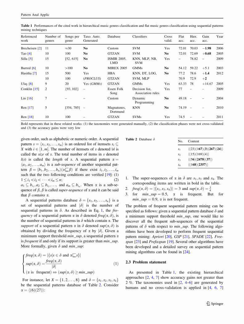
3.4.3 Second transformation with the K-NN algorithm
The first transformation of a song using the K-NN algo-
rithm with ðK[ 1Þ is limited for high values of K. Indeed,
if the value of K is large, the itemset corresponding to any
vector vj of music descriptors may always be
ðg1; g2; . . .; gNÞ because all the N genres may be found in
the neighborhoods of vj, but not in the same proportions. In
such a situation, the same sequential pattern may be gen-
erated for each training song. This limitation comes from
the fact that the number of central vectors of the genres
appearing in the neighborhoods vj is not considered during
the transformation. As shown in Fig. 6, the itemsets asso-
ciated with vectors v1 and v3 are the same (composed of
squares and circles) when the first transformation is
applied, but they are different with the second transfor-
mation. According to this figure, the song c can therefore
be seen as a sequence of Histograms ðH1H2. . .HwÞ. Eachhistogram Hj is having N bins fg1; g2; . . .; gNg and the
height of bin k (namely HjðkÞ) is the number of central
vectors of genre gk found in the neighborhoods of vector vj.
To avoid the situation where HjðkÞ ¼ 0 in the histogram, 1
is intentionally added to the number of central vectors of
genre gk found in the neighborhoods the vector vj. With
this last transformation, one will need to mine sequences of
frequent histograms to derive the vector of descriptors of
each genre.
Histograms (colour histograms) are widely used in
image and video information retrieval. Surveys on the
theory and applications of image and video mining tech-
niques are respectively proposed in [29, 30]. In [31], Fer-
nando performed frequent itemset mining for image
classification. In that work, he proposed a simple method to
convert a local colour histogram of an image into a
Fig. 4 Transformation of a song with the NN approach. Squares,
circles and triangles represent respectively the central vectors of 3
genres g1; g2 and g3
Fig. 5 First transformation of a song with the K-NN approach
(K ¼ 4). Squares, circles and triangles represent respectively the
central vectors of 3 genres g1; g2 and g3
Pattern Anal Applic
123
particular type of itemset. A similar method is applied in
this paper to convert sequences of histograms into
sequential patterns as presented in Fig. 6. This transfor-
mation enables to mine frequent sequences of histograms
with common sequential pattern mining algorithms. In
order to transform the sequence of histograms
ðH1H2. . .HwÞ of a song c into a sequential pattern, one can
proceed as follows:
1. An item is now considered as a pair (g, y), g being a
genre label and y a positive integer.
2. The kth bin of histogram Hj is converted into the item
ðgk;HjðkÞÞ.3. Histogram Hj becomes the itemset sj ¼ fðgk;HjðkÞÞg
with k ¼ 1. . .N.
4. The sequence of histograms ðH1H2. . .HwÞ of c becomes
the sequential pattern hðs1Þðs2Þ. . .ðswÞi where each sj is
the itemset derived from Hj.
One can observe that with this transformation, the resulting
sequential patterns are composed of itemsets containing
always exactly N items. This was not the case with the first
transformation with the K-NN algorithm (K[ 1). In these
conditions, an itemset sj1 is included in another itemset sj2(i.e: sj1 � sj2Þ if ðHj1ðkÞ�Hj2ðkÞÞ for k ¼ 1. . .N. The other
concepts (sub-sequence, super-sequence, support, frequent
sequence, etc.) previously defined in Sect. 2.2 remain the
same. All the common sequential pattern mining algorithms
can be adapted to mine frequent histograms. This can be
done by filtering the output of the considered algorithm so
that only sequences composed of itemsets containing exactly
N items are taken into account. This allows to remain con-
sistent with the methodology because adapted versions of
common sequential pattern mining algorithms are finally
used to mine frequent sequences of histograms. In the rest of
the paper, the first and the second K-NN transformations
ðK[ 1Þ will be, respectively, referenced as the K-NN
approach and the histogram approach.
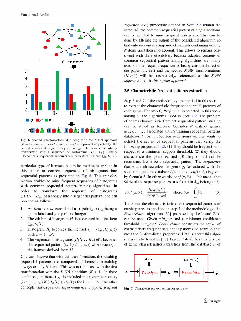
3.5 Characteristic frequent patterns extraction
Step 6 and 7 of the methodology are applied in this section
to extract the characteristic frequent sequential patterns of
each genre. For step 6, Prefixspan is selected in this work
among all the algorithms listed in Sect. 2.2. The problem
of genres characteristic frequent sequential patterns mining
can be stated as follows: Consider N distinct genres
g1; g2; . . .; gN associated with N training sequential patterns
databases d1; d2; . . .; dN . For each genre gi, one wants to
extract the set ui of sequential patterns that verify the
following properties [32]: (1) They should be frequent with
respect to a minimum support threshold, (2) they should
characterize the genre gi, and (3) they should not be
redundant. Let a be a sequential pattern. The confidence
that a can characterize the genre gi (associated with the
sequential patterns database di) denoted conf ða; diÞ is givenby formula 3. In other words, conf ða; diÞ ¼ 0:9 means that
90 % of the super-sequences of a found in dall belong to di.
conf ða; diÞ ¼freqða; diÞfreqða; dallÞ
where dall ¼[N
i¼1
di ð3Þ
To extract the characteristic frequent sequential patterns of
music genres as specified in step 7 of the methodology, the
FeatureMine algorithm [32] proposed by Lesh and Zaki
can be used. Given min sup and a minimum confidence
threshold min conf , FeatureMine constructs the set ui of
characteristic frequent sequential patterns of genre gi that
meet the 3 afore-listed properties. Details about this algo-
rithm can be found in [32]. Figure 7 describes this process
of genre characteristics extraction from the database di of
Fig. 6 Second transformation of a song with the K-NN approach
(K ¼ 4). Squares, circles and triangles represent respectively the
central vectors of 3 genres g1; g2 and g3. The song c is initially
transformed into a sequence of histograms ðH1. . .H5Þ. Finally
c becomes a sequential pattern where each item is a pair ðgk;HjðkÞÞ
Fig. 7 Characteristics extraction for genre gi
Pattern Anal Applic
123

genre gi. Generally for N genres, it is advised to set
min conf to 1Nfor each genre [32]. This value is adopted in
the rest of this paper.
3.6 Vector associated with a genre
This section details the 8th step of the methodology by
computing a new descriptor for each genre. Consider a
song c associated with the sequential pattern Sc. Let ui ¼ffi1; fi2; . . .; fijuijg be the set of characteristic sequential
patterns of gi output by FeatureMine. The song c is rep-
resented as the vector c!¼ ðx1ðcÞ; . . .;xNðcÞÞ where eachxiðcÞ is the percentage of the characteristic frequent
sequences of the genre gi contained in Sc as shown in
Eq. 4. For instance, c!¼ ð0:55; 0:67; 0:75Þ means that
c contains 55 % of the characteristic sequences of genre g1,
67 % of the characteristic sequences of genre g2 and 75 %
of the characteristic sequences of genre g3.
xiðcÞ ¼Pjuij
j¼1 yijðcÞjuij
with yijðcÞ ¼1 if fijYSc
0 otherwise
�
ð4Þ
The proposed descriptor of genre gi is the vector Ui�! ¼
ðh1ðgiÞ; . . .; hNðgiÞÞ where each hjðgiÞ is the normalized
sum of the jth components of the vectors c! associated with
the songs c 2 di as shown in Eq. 5.
hjðgiÞ ¼100
jdijX
c2dixjðcÞ
!
ð5Þ
According to this representation, Ui�! ¼ ð40; 75; 55Þ means
that genre gi contains 40 % of the characteristic sequences
of genre g1, 75 % of the characteristic sequences of genre
g2, and 55 % of the characteristic sequences of genre g3.
3.7 Taxonomies generation
This section is devoted to the taxonomy generation as
specified in step 9 of the methodology. To achieve this
goal, the similarity between two genres must first be
computed. In this work, the similarity between two music
genres is considered as the mathematical distance
between their associated vectors. The 4 following dis-
tances have been selected: Euclidean distance de, Man-
hattan distance dm, Tchebychev distance dt and Cosine
distance da extracted from the dot product of their asso-
ciated vectors. Equation 6 shows how to compute these
distances for two vectors Ui�! ¼ fui1; ui2; . . .; uiNg and
Uj�! ¼ fuj1; uj2; . . .; ujNg, respectively associated with
genres gi and gj.
deð Ui�!
; Uj�!Þ ¼
ffiffiffiffiffiffiffiffiffiffiffiffiffiffiffiffiffiffiffiffiffiffiffiffiffiffiffiffiffiffiffi
XN
k¼1
uik ujk� �2
vuut (Euclidean)
dmð Ui�!
; Uj�!Þ ¼
XN
k¼1
uik ujk��
�� (Manhattan)
dtð Ui�!
; Uj�!Þ ¼ max
1� k�Nuik ujk��
�� (Tchebychev)
dað Ui�!
; Uj�!Þ ¼ arccos
Ui�!
: Uj�!
j Ui�!j:j Uj
�!j
!
(Cosine)
ð6Þ
The similarity between two genres allows to perform the
hierarchical clustering of music genres. The similarity
matrix (square and symmetric) between all the genres gi 2G is first built. This matrix will then enable us to realize the
hierarchical clustering of the N genres. This operation can
easily be realized by the AHC [9] algorithm that outputs a
detailed dendrogram of the N genres from which the tax-
onomy can be derived. The principle of this algorithm is as
follows: initially, each genre gi is considered as a cluster of
size 1. At each step, the two closest clusters are found and
merged into a new cluster. The process is repeated until
one single cluster is obtained. AHC involves the existence
of a distance measure between two clusters. There exist
several possible distances between clusters. The 4 follow-
ing distances have been considered in this work: the min-
imum, the centroid, the average and the maximum
distances.
4 Experimental results
4.1 Experiments on GTZAN
The proposed method was experimented on the GTZAN
database [25] composed of 10 music genres: blues,
classical, country, disco, hiphop, jazz, metal, pop, reg-
gae and rock. In the rest of the paper, these genres will,
respectively, be represented in figures by the acronyms:
bl, cl, co, di, hi, ja, me, po, re and ro. Each genre being
represented by 100 ‘.wav’ files (30 s, 22,050 Hz, 32 bits
floating point, mono). It is important to note that 7.2 %
of the excerpts of GTZAN come from the same
recording (including 5 % being exact duplicates) and
10.8 % of the database is mislabelled [33]. The 9 first
steps of the methodology have been applied to GTZAN
as follows:
Steps 1–3: To compute the music descriptors listed in
Sect. 3.3, each music excerpt was split into windows of
about 20 ms, each window having 512 samples with an
overlap of 50 % between two consecutive windows. The
Pattern Anal Applic
123
mean of the music features was calculated for each texture
window of one second.
Steps 4–5: To transform a song into a sequential pat-
tern, the k-means algorithm was applied to generate
k central vectors per genre. Experiments are realized
in [34] to select a suitable value of k. In that paper, it was
proposed to apply the k-means algorithm to transform a
music excerpt into a Markov chain of genres. To select the
value of k, flat classification experiments on a dataset
composed of 10 music genres including 4 Cameroonian
genres were performed. Up to 30 different values of
k taken between 5 and 150 with a step of 5 were tested.
The training was done with 90 songs per genre, and 10
songs were used per genre for the flat classification stage.
The highest accuracy value (84 %) was reached for k ¼95 and k ¼ 100. It is according to these experiments that
k is set to 100 in this paper.
The K-NN approach was applied for K ¼ 6; 7; 8; 9; 10,
and the histogram approach for K ¼ 50 and K ¼ 100. This
enabled us to analyze the impact of the value of K on the
vector descriptor U!
of genres. After these analysis, only
the values K ¼ 10 and K ¼ 50 were finally selected,
respectively, for the K-NN and histogram approaches
during the taxonomy generation.
With the simple NN approach, each training song of
30 s was then transformed into a sequential pattern. In
contrast, the length of the sequential patterns generated
with the K-NN and the histogram approaches was too
large (hundreds of items). Under such conditions, Pre-
fixSpan can generate millions of sequences if the whole
song is considered. For this reason, every training song of
30 s was split into 6 consecutive songs of 5s each before
being converted into a sequential pattern. The maximum
length of the generated sequences decreased from 300 to
50 items.
Steps 6–7: Adapted versions of PrefixSpan and Fea-
tureMine were developed in C language. After setting
min conf to 110
(because GTZAN has 10 genres), the pro-
cess described in Fig. 7 was applied by successively exe-
cuting the PrefixSpan and FeatureMine on GTZAN. The
minimum support threshold varied from one transformation
to another in order to extract a reasonable number of
characteristic sequential patterns per genre. Table 3 shows
the number of characteristic frequent sequential patterns
found for each genre. In this table, the K-NN approach is
applied with K ¼ 10 and the histogram approach is applied
with K ¼ 50.
Step 8: The vectors associated with the various genres
were later calculated as explained in Sect. 3.6. Each line of
Table 4a–h shows the components of the vector associated
with the corresponding genre in GTZAN. Table 4a reveals
that with the NN algorithm, in the vector representing a
genre gi, the dominant component is always the ith com-
ponent. This is a nice coherence property that is not sat-
isfied by the other approaches.
The vector descriptors obtained with the K-NN approach
were calculated for K ¼ 6; . . .; 10, and a particular config-
uration was observed for K ¼ 7; 9; 10 respectively as shown
in Table 4b–d: the vectors representing country, reggae and
rock were dominated by the component corresponding to
blues. The same situation occurred in the vectors of disco
and metal that were dominated by their components corre-
sponding to hiphop. These confusions may be due to the
strong timbre similarities existing between these genres.
Therefore, it is possible to deduce that these genres may
later belong to the same clusters in the resulting taxonomy.
This observation led to the selection of the value K ¼ 10
during the taxonomy generation.
Similarly, the value K ¼ 50 was selected for the his-
togram approach because in Table 4e–f, the vector de-
scriptors are similar for K ¼ 50 and K ¼ 100. In these
tables, the vectors representing classical and jazz are
dominated by the component corresponding to country.
Thus, one can guess that these 3 genres may belong to the
same cluster and this was later observable in the resulting
taxonomy.
Step 9: From the vector representation, the distance
matrix between the genres of GTZAN is calculated using
the 4 distances described in Sect. 3.7. Finally, the AHC
clustering algorithm was applied to realize the hierarchical
clustering and generate dendrograms from which a taxon-
omy was extracted. The 4 cluster distances presented in
Sect. 3.7 were used to achieve this goal. These pairs of
distance measures generated the 6 dendrograms presented
in Fig. 8a–f. Table 5a–c specify the dendrogram generated
by each pair, respectively, for the NN, the K-NN (K ¼ 10)
and the histogram (K ¼ 50) approaches.
The contents of dendrograms DG1, DG2 and DG3 are
similar. From these 3 dendrograms generated by the NN
and the K-NN approaches, the taxonomy T1 of GTZAN
presented in Fig. 9a was derived. The histogram approach
generated dendrograms DG4, DG5 and DG6. DG4 is not
similar to DG5 and DG6. DG5 and DG6 are quite similar,
only the location of genre pop changes from DG5 to DG6.
Table 3 Number of frequent characteristic sequences extracted by
FeatureMine for the genres of GTZAN
bl cl co di hi ja me po re ro
NN 146 871 193 301 244 271 198 391 194 243
K-NN 82 487 154 755 274 707 1618 577 170 597
Histo. 96 226 75 74 110 190 119 166 77 42
Pattern Anal Applic
123

Table 4 Genres vectors in GTZAN (one vector per line)
bl cl co di hi ja me po re ro
(a)—Simple NN with min sup ¼ 0:5
bl 59.6 6.4 51.6 37.4 39.5 26.7 33.1 24.5 46.8 46.2
cl 21.6 60.1 28.1 4.9 5.5 56.1 4.3 2.6 18.9 12.0
co 56.8 15.4 59.3 33.0 35.6 37.2 33.1 17.3 53.8 48.4
di 41.7 1.8 35.7 59.2 57.8 8.5 57.2 43.6 43.8 50.1
hi 40.7 1.8 35.2 54.1 59.0 8.8 50.2 44.6 43.0 47.6
ja 38.8 34.8 44.1 14.1 14.1 59.4 15.7 5.6 35.1 26.5
me 34.2 0.5 26.9 50.8 50.1 3.9 59.9 36.6 36.0 45.0
po 35.0 2.8 26.6 49.4 52.6 7.4 39.2 58.1 31.1 36.2
re 51.0 5.1 52.5 37.6 39.8 21.1 38.2 23.4 59.7 52.0
ro 52.7 5.3 50.1 45.6 46.5 18.8 47.4 26.8 56.2 60.1
(b)—K-NN approach with K ¼ 7 and min sup ¼ 0:75
bl 82.7 53.5 75.6 56.2 63.0 59.5 47.9 45.0 69.6 69.2
cl 56.7 81.2 59.9 11.2 14.4 75.6 7.7 5.7 37.7 33.2
co 82.3 60.5 81.4 51.4 56.9 66.5 43.8 34.4 75.8 72.5
di 73.3 18.2 62.1 81.1 82.1 27.2 75.9 69.8 70.1 71.6
hi 72.3 21.9 59.5 76.8 81.2 29.6 70.0 72.1 66.6 68.5
ja 73.5 78.6 77.4 27.7 32.5 80.8 22.8 15.7 61.4 55.9
me 71.1 12.7 57.5 81.7 81.9 21.3 81.1 69.2 66.2 69.6
po 61.5 17.4 46.4 74.7 79.5 22.4 66.5 80.4 54.0 56.5
re 80.9 44.1 78.2 62.9 69.0 53.4 55.2 47.8 80.3 77.0
ro 85.1 38.4 80.2 68.9 73.4 49.0 63.2 51.0 82.4 81.9
(c)—K-NN approach with K ¼ 9 and min sup ¼ 0:85
bl 90.5 62.4 86.1 63.8 72.4 67.6 53.6 57.0 82.5 75.9
cl 66.7 88.7 68.9 15.0 20.9 84.6 9.6 9.1 49.4 40.9
co 90.1 71.0 89.4 59.6 67.8 75.0 49.7 47.1 85.3 79.6
di 84.3 25.8 76.9 88.9 90.9 35.2 83.2 83.6 83.0 78.1
hi 83.6 29.7 74.8 84.3 88.9 36.8 77.7 82.0 80.1 75.1
ja 83.4 87.9 85.3 34.2 43.6 89.0 27.6 25.1 73.0 65.4
me 85.2 18.7 76.7 88.8 91.1 27.9 89.1 83.3 82.8 78.3
po 74.8 22.4 63.0 82.6 87.3 27.1 76.4 88.2 69.8 62.6
re 89.3 56.4 87.1 72.8 79.5 64.1 63.6 61.6 88.5 83.6
ro 93.3 48.8 91.1 78.2 83.9 58.1 71.5 66.7 92.0 89.3
(d)—K-NN approach with K ¼ 10 and min sup ¼ 0:85
bl 90.0 59.9 85.1 60.6 70.5 65.4 52.2 54.7 81.3 74.4
cl 64.4 88.8 68.0 12.9 19.7 83.8 8.5 8.6 45.4 36.5
co 90.4 69.8 89.2 56.2 65.9 74.9 47.5 44.9 83.7 77.9
di 85.9 23.6 77.0 88.5 90.6 33.4 83.5 83.5 84.9 79.2
hi 85.1 27.2 75.0 83.4 88.3 35.0 77.6 81.3 82.2 76.1
ja 82.0 87.7 84.4 31.5 41.3 88.7 25.9 23.9 69.5 60.9
me 85.8 16.2 75.4 88.9 91.0 25.0 88.6 84.8 84.6 79.3
po 75.4 20.1 62.1 81.0 86.2 25.5 75.8 87.9 72.6 62.6
re 89.4 53.7 86.2 71.0 78.9 62.5 62.9 60.9 88.6 83.0
ro 94.0 45.5 90.1 77.5 83.4 55.6 70.9 66.5 92.2 89.0
(e)—Histogram approach with K ¼ 50 and min sup ¼ 0:005
bl 1.34 0.47 0.99 0.42 0.42 0.59 0.32 0.31 0.33 0.19
cl 1.34 1.74 2.14 0.01 0.02 1.59 0.02 0.01 0.18 0.16
co 0.59 0.43 1.17 0.20 0.18 0.53 0.12 0.10 0.28 0.30
di 0.24 0.02 0.12 0.95 0.55 0.05 0.49 0.41 0.39 0.25
hi 0.33 0.05 0.19 0.73 0.99 0.09 0.60 0.58 0.48 0.23
Pattern Anal Applic
123

But this difference cannot be neglected. Thus the 3 tax-
onomies T2; T3 and T4 of GTZAN presented in Fig. 9b–d
are, respectively, derived from dendrograms DG4, DG5 and
DG6.
4.2 Experiments on GTZAN1
In order to experience the consistency of the proposed
method, experiments have been realized on a new
database composed of a combination of GTZAN and 5
Afro genres. The proposed name of this new database is
GTZAN?. The 5 new genres are: bikutsi, makossa,
bamileke, salsa and zouk. In the rest of the paper, these 5
genres will be represented in figures by the acronyms: bi,
ma, ba, sa and zo. Each Afro genre was represented by
100 ‘.wav’ files of 30 s each with the same properties as
those of GTZAN. Zouk is a French-Caribbean genre and
salsa is a genre having Cuban origins, but here many
Table 4 continued
bl cl co di hi ja me po re ro
ja 1.00 0.90 1.52 0.10 0.06 1.31 0.10 0.02 0.24 0.37
me 0.23 0.01 0.06 0.69 0.68 0.05 1.02 0.55 0.43 0.16
po 0.40 0.06 0.14 0.88 1.38 0.08 1.12 1.53 0.68 0.13
re 0.28 0.12 0.29 0.46 0.41 0.20 0.37 0.30 0.89 0.43
ro 0.26 0.13 0.35 0.32 0.25 0.23 0.24 0.15 0.38 0.74
(f)—Histogram approach with K ¼ 100 and min sup ¼ 0:005
bl 1.42 0.44 1.31 0.44 0.45 0.61 0.30 0.31 0.29 0.21
cl 1.41 1.82 2.32 0.02 0.03 1.79 0.02 0.02 0.13 0.14
co 0.70 0.43 1.27 0.21 0.19 0.52 0.12 0.10 0.16 0.19
di 0.30 0.02 0.09 0.97 0.62 0.05 0.46 0.42 0.41 0.29
hi 0.40 0.05 0.18 0.78 1.04 0.07 0.57 0.59 0.48 0.31
ja 1.02 0.95 1.63 0.07 0.05 1.36 0.09 0.01 0.12 0.28
me 0.23 0.01 0.07 0.66 0.72 0.05 1.01 0.56 0.55 0.30
po 0.49 0.05 0.15 1.07 1.52 0.06 1.21 1.54 0.89 0.12
re 0.25 0.11 0.20 0.41 0.39 0.15 0.35 0.29 0.83 0.32
ro 0.25 0.12 0.27 0.32 0.27 0.19 0.24 0.15 0.27 0.75
The highest component of each vector is bold
Fig. 8 Automatically generated dendrograms of GTZAN. a Dendrogram DG1. b Dendrogram DG2. c Dendrogram DG3. d Dendrogram DG4.
e Dendrogram DG5. f Dendrogram DG6
Pattern Anal Applic
123

salsa samples played by Cameroonian singers have been
included. The 3 remaining new genres are Cameroonian
genres, and their short descriptions can be found
online [35].
The first nine steps of the methodology followed in
Sect. 4.1 for GTZAN have been followed for GTZAN?.
However, at step 7, min conf was set to 115for FeatureMine
because GTZAN? has 15 genres. As it was done on
GTZAN, the associated vectors of each genre were cal-
culated and the AHC algorithm was applied to generate
dendrograms. Due to space constraints, only the NN and
the K-NN approaches are presented for GTZAN?. For the
same reason, the components of the vectors associated with
the genres of GTZAN? are not presented. The number of
characteristic sequences extracted by FeatureMine for each
genre is presented in Table 6. The 4 dendrograms presented
in Fig. 10a–d were obtained for GTZAN?. Table 7 spec-
ifies the dendrogram generated by each pair of distance
measures for the NN approach. The dendrogram DG03
presented in Fig. 10c was generated for all the 16 pairs of
distances with the K-NN approach (K ¼ 10). From the
general shapes of these automatically generated dendro-
grams, the taxonomy T 0 of GTZAN? presented in Fig. 11
was derived.
4.3 Properties of the generated taxonomies
The taxonomies of GTZAN generated by the proposed
method share some similarities with the existing tax-
onomies presented in Fig. 1b–f [4, 7, 8]. Additionally, the
proposed method generates taxonomies satisfying the fol-
lowing criteria proposed by Pachet in [10]:
1. Objectivity: The proposed method generates objective
taxonomies because a taxon is a music genre defined as
a vector composed of N elements calculated with
Eq. 5.
2. Similarity: The proposed taxonomies allow search by
similarity because if two genres of G belong to the
same cluster, their associated vectors are close with
respect to the similarity measure.
Table 5 Dendrograms generated on GTZAN
de dm dt da
(a) The NN approach
Max DG2 DG2 DG2 DG2
Ave DG2 DG1 DG2 DG2
Cen DG1 DG1 DG1 DG1
Min DG3 DG3 DG3 DG1
(b) The K-NN approach (K ¼ 10)
Max DG2 DG2 DG1 DG2
Ave DG2 DG2 DG1 DG2
Cen DG2 DG2 DG1 DG2
Min DG3 DG3 DG3 DG1
(c) The histogram approach (K ¼ 50)
Max DG6 DG5 DG5 DG4
Ave DG5 DG5 DG6 DG4
Cen DG6 DG5 DG6 DG4
Min DG5 DG5 DG6 DG4
Fig. 9 Proposed taxonomies T1;T2;T3 and T4 of GTZAN. T1 is
generated by the NN and the K-NN approaches. T2; T3 and T4 are
generated by the histogram approach. a Taxonomy T1. b Taxonomy
T2. c Taxonomy T3. d Taxonomy T4
Table 6 Number of frequent characteristic sequences extracted by
FeatureMine for the genres of GTZAN?
bi bl cl co di hi ja ma
NN 226 39 812 72 96 97 189 82
K-NN 540 10 450 28 53 26 234 46
me ba po re ro sa zo
NN 87 192 127 80 68 140 133
K-NN 82 124 84 22 41 402 542
Pattern Anal Applic
123

3. Consistency: The proposed taxonomies are consistent
because the semantic of the links remains the same
throughout the taxonomies.
4. Evolutivity: As it can be observed in Figs. 9a and 11,
the taxonomy of GTZAN generated by the NN and the
K-NN approaches is preserved in the taxonomy of
GTZAN? generated by these approaches. Therefore
the proposed method is experimentally evolutive
because it is capable to cope with new genres.
4.4 Time performance for dendrogram generation
The proposed taxonomies were generated off-line and once
on a personal computer having the following properties: (1)
Processors: Intel(R) Core(TM) i7-2670QM CPU @2.2GHz
2.2GHz (2) RAM: 8 GB. Table 8 gives details about the
maximum time taken to generate a dendrogram.
4.5 Hierarchical genres classification
This section shows how to perform the hierarchical classi-
fication which is the last step of the methodology. Experi-
ments on flat and hierarchical classifiers were performed
using the MEKA [36] data mining tool. Recently developed
in 2014, MEKA is an extension of WEKA [12] that enables
multi-label classification. A detailed evaluation and analy-
sis of some of the main multi-label classification methods in
MIR can be found in [37]. MEKA was selected because it
includes a meta classifier named HASEL that enables the
user to clearly specify a taxonomy in an ‘.arff’ file. Then the
user selects a basic WEKA classifier to be applied with this
taxonomy. HASEL partitions labels into subsets based on
the defined hierarchy. It assumes that a dot ‘.’ in the attri-
bute name defines hierarchical branches. Figure 12 presents
the header of the ‘.arff’ file in which the taxonomy of
GTZAN was described.
Several music genres classifiers are presented in [38].
The 4 following basic classifiers have been selected (their
WEKA/MEKA corresponding names are in brackets):
SVMs with polynomial kernels (SMO), Multi Layers Per-
ceptrons (MLP), Decision Trees (J48) and KNNs (IBk). All
these classifiers were used with their default settings in
MEKA. After a 10-fold cross-validation (90–10 %), the
results presented in Table 9a–b were obtained for GTZAN
and GTZAN?.
Experimental results show that the hierarchical classifiers
based on the proposed taxonomies always outperform the
corresponding flat classifiers. The best classification results
were obtained with the MLP and SMO classifiers in the two
Fig. 10 Automatically generated dendrograms of GTZAN?. a Dendrogram DG01. b Dendrogram DG0
2. c Dendrogram DG03. d Dendrogram DG0
4
Table 7 Dendrograms of GTZAN? with the NN
de dm dt da
max DG03 DG0
3 DG01 DG0
3
ave DG01 DG0
3 DG04 DG0
1
cen DG01 DG0
3 DG04 DG0
1
min DG02 DG0
2 DG04 DG0
2
Fig. 11 Proposed taxonomy T 0 of GTZAN?
Pattern Anal Applic
123

experimental databases with accuracies greater than 80 %.
However, classification with MLP took several hours unlike
the other classifiers for which just a couple of seconds was
needed. Hierarchical classification based on IBk and SMO
always showed minimum accuracy gains close to 10 %. The
minimum accuracy gains provided by J48 classifier are
always close to 20 % and MLP gave minimum accuracy
gains reaching 40 % in GTZAN?. Additionally, the hier-
archical classification accuracies are close for GTZAN?
and GTZAN. This can be explained by the fact that the
proposed method generated evolutive taxonomies for the
NN and the K-NN approaches.
In fact, 45of the new added Afro genres are gathered in
the same cluster C3 in the taxonomy T 0 of GTZAN?.
Therefore, a single classifier is trained and dedicated to
separate them at this level. This reduces considerably the
error rate for these 4 new genres. The preservation of the
taxonomy T1 of GTZAN implies that almost all the songs
that were accurately classified in GTZAN were also
accurately classified in GTZAN?.
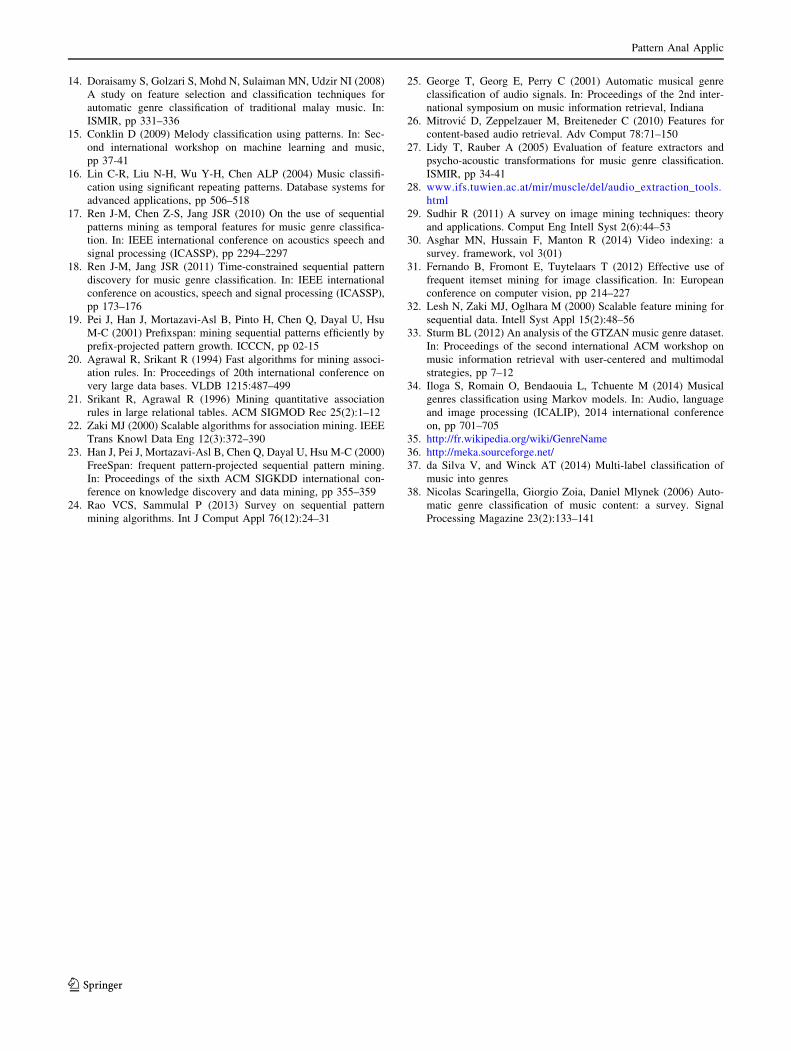
4.6 Comparisons with related work
The taxonomy proposed here for GTZAN has been com-
pared with the taxonomies of Fig. 1b, e, f (genre ‘blues’
excluded) used, respectively, in [4, 7, 8]. The best hierar-
chical classification performance of this work was com-
pared with those in these three papers. To make
comparisons with [8] in which only 9 genres of GTZAN
are considered, a new taxonomy T 01 was generated for the
database GTZAN blues (GTZAN without the genre ‘blues’)
using the NN and the K-NN approaches. The resulting
taxonomy T 01 was almost identical to T1 presented in
Fig. 9a with ‘blues’ removed from cluster C3. Table 10
gives details about the hierarchical classification results on
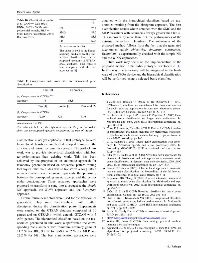
GTZAN blues based on the approach.
As shown in Table 11a, the best performance (85.3 %)
obtained by the approach proposed here with MLP clearly
improves the best performance (78 %) obtained in [8].
Table 11b shows comparisons for GTZAN. These com-
parisons show that the hierarchical classifiers proposed in
this work outperform with more than 7 % the results pre-
sented in [4, 7, 8].
5 Conclusion
The new radio prototype based on FPGA technologies
developed in [1] is already able to perform the concurrent
demodulation of entire broadcast bands. But music genre
Table 8 Time performance for
dendrogram generationStep Max. time Result
Descriptors extraction �5 s/song 1 Sequence of vectors of descriptors/song
k-means �2 min/genre 100 central vectors/genre
K-NN �1 s/song 1 sequential pattern/song
PrefixSpan �(around 15 min)/genre 1 sequential pattern database/genre
FeatureMine �(1 h) Many characteristics for each genre
Genre vector �1 s/genre 1 vector/genre
AHC �1 s 1 dendrogram
Fig. 12 Headers of the ‘arff’ file describing the proposed taxonomy
of GTZAN in MEKA
Table 9 Classification results with IBk = KNNs, SMO = SVMs with
polynomial kernels, MLP = Multi Layers Perceptrons, J48 = Decision
Trees
Flat T1 T2 T3 T4 Min Gain
(a) Results in GTZAN
IBk 63.8 74.2 77.3 81.6 84.4 ?10.4
SMO 72.3 81.7 85.5 90.2 91.2 ?9.4
MLP 68.4 85 87.4 90.9 91.6 ?16.6
J48 47.3 67.7 68.5 76.1 79.3 20.4
Flat T 0 Gain
(b) Results in GTZAN?
IBk 65.4 77.1 ?11.7
SMO 75.5 85.2 ?9.7
MLP 41.9 82.1 ?40.2
J48 47.3 69.5 ?22.2
Accuracies are in (%)
Pattern Anal Applic
123
classification is not yet applicable in that prototype. Several
hierarchical classifiers have been developed to improve the
efficiency of music recognition systems. The goal of this
work was to provide hierarchical classification with bet-
ter performances than existing work. This has been
achieved by the proposal of an automatic approach for
taxonomy generation based on sequential pattern mining
techniques. The main idea was to transform a song into a
sequence where each element represents the proximity
between the corresponding music excerpt and the genres
under consideration. Three separated approaches were
proposed to transform a song into a sequence: the simple
NN approach, the K-NN approach and the histogram
approach.
Timbre music descriptors were used for the taxonomies
generation. They were then combined with rhythm
descriptors during the classification phase. Experiments
were carried on the GTZAN database composed of 10
genres and on GTZAN? which extends GTZAN with 5
Afro genres. The hierarchical classifiers based on the tax-
onomies generated in this work outperformed the corre-
sponding flat classifiers with minimum accuracy gains of
11.7 % for IBk, 9.7 % for SMO, 40.2 % for MLP and
22.2 % for J48. The best classification accuracies were
obtained with the hierarchical classifiers based on tax-
onomies resulting from the histogram approach. The best
classification results where obtained with the SMO and the
MLP classifiers with accuracies always greater than 80 %.
This improves by more than 7 % the performances of the
existing hierarchical classifiers. The robustness of the
proposed method follows from the fact that the generated
taxonomies satisfy objectivity, similarity, consistency.
Evolutivity is experimentally checked with the simple NN
and the K-NN approaches.
Future work may focus on the implementation of the
proposed method in the radio prototype developed in [1].
In this way, the taxonomy will be integrated in the hard-
ware of the FPGA device and the hierarchical classification
will be performed using a selected basic classifier.
References
1. Tietche BH, Romain O, Denby B, De Dieuleveult F (2012)
FPGA-based simultaneous multichannel fm broadcast receiver
for audio indexing applications in consumer electronics scenar-
ios. IEEE Trans Consum Electron 58(4):1153–1161
2. Brecheisen S, Kriegel H-P, Kunath P, Pryakhin A (2006) Hier-
archical genre classification for large music collections. In:
Multimedia and expo, 2006 IEEE international conference on,
pp 1385–1388
3. Costa E, Lorena A, Carvalho ACPLF, Freitas A (2007) A review
of performance evaluation measures for hierarchical classifiers.
In: Evaluation methods for machine learning II: papers from the
AAAI-2007 workshop, pp 1–6
4. Li T, Ogihara M (2005) Music genre classification with taxon-
omy. In: Acoustics, speech, and signal processing, 2005. In:
Proceedings.(ICASSP’05). IEEE international conference on, vol.
5, pp. v-197
5. Silla Jr CN, Freitas A et al (2009) Novel top-down approaches for
hierarchical classification and their application to automatic music
genre classification. In: Systems, man and cybernetics, 2009. SMC
2009. IEEE international conference on, pp 3499–3504
6. Burred JJ, Lerch A (2003) A hierarchical approach to automatic
musical genre classification. In: Proceedings of the 6th interna-
tional conference on digital audio effects, pp 8–11
7. Ariyaratne HB, Zhang D (2012) A novel automatic hierarchical
approach to music genre classification. In: Multimedia and expo
workshops (ICMEW), 2012 IEEE international conference on,
pp 564–569
8. Bagcı U, Erzin E (2005) Boosting classifiers for music genre
classification. Comput Inf Sci-ISCIS 2005:575–584
9. Shao X, Xu C, Kankanhalli MS (2004) Unsupervised classifica-
tion of music genre using hidden markov model. In: Multimedia
and expo, 2004. ICME’04. 2004 IEEE international conference
on, vol 3, pp 2023–2026
10. Pachet F, Cazaly D et al (2000) A taxonomy of musical genres.
RIAO, pp 1238–1245
11. http://marsyasweb.appspot.com/download/data_sets/
12. Witten IH, Frank E (2005) Data mining: practical machine
learning tools and techniques
13. Aggarwal CC, Wolf JL, Yu PS, Procopiuc C, Park JS (1999) Fast
algorithms for projected clustering. ACM SIGMoD Rec
28(2):61–72
Table 10 Classification results
in GTZANblues with IBk =
KNNs, SMO = SVMs with
polynomial kernels, MLP =
Multi Layers Perceptrons, J48 =
Decision Trees
T 01
IBk 75.7
SMO 83.7
MLP 85.3
J48 69.4
Accuracies are in (%)
The value in bold is the highest
accuracy produced by the hier-
archical classifier based on the
proposed taxonomy of GTZAN,
blues excluded. This value is
later compared with the best
accuracy in [8]
Table 11 Comparisons with work cited for hierarchical genre
classification
Ulas [8] This work T 01
(a) Comparisons in GTZAN blues
Accuracy 78 85.3
Tao [4] Hasitha [7] This work T4
(b) Comparisons in GTZAN
Accuracy 72.69 72.9 91.6
Accuracies are in (%)
The values in bold are the highest accuracies. They are in bold to
show that the proposed approach outperforms the state of the art
Pattern Anal Applic
123
14. Doraisamy S, Golzari S, Mohd N, Sulaiman MN, Udzir NI (2008)
A study on feature selection and classification techniques for
automatic genre classification of traditional malay music. In:
ISMIR, pp 331–336
15. Conklin D (2009) Melody classification using patterns. In: Sec-
ond international workshop on machine learning and music,
pp 37-41
16. Lin C-R, Liu N-H, Wu Y-H, Chen ALP (2004) Music classifi-
cation using significant repeating patterns. Database systems for
advanced applications, pp 506–518
17. Ren J-M, Chen Z-S, Jang JSR (2010) On the use of sequential
patterns mining as temporal features for music genre classifica-
tion. In: IEEE international conference on acoustics speech and
signal processing (ICASSP), pp 2294–2297
18. Ren J-M, Jang JSR (2011) Time-constrained sequential pattern
discovery for music genre classification. In: IEEE international
conference on acoustics, speech and signal processing (ICASSP),
pp 173–176
19. Pei J, Han J, Mortazavi-Asl B, Pinto H, Chen Q, Dayal U, Hsu
M-C (2001) Prefixspan: mining sequential patterns efficiently by
prefix-projected pattern growth. ICCCN, pp 02-15
20. Agrawal R, Srikant R (1994) Fast algorithms for mining associ-
ation rules. In: Proceedings of 20th international conference on
very large data bases. VLDB 1215:487–499
21. Srikant R, Agrawal R (1996) Mining quantitative association
rules in large relational tables. ACM SIGMOD Rec 25(2):1–12
22. Zaki MJ (2000) Scalable algorithms for association mining. IEEE
Trans Knowl Data Eng 12(3):372–390
23. Han J, Pei J, Mortazavi-Asl B, Chen Q, Dayal U, Hsu M-C (2000)
FreeSpan: frequent pattern-projected sequential pattern mining.
In: Proceedings of the sixth ACM SIGKDD international con-
ference on knowledge discovery and data mining, pp 355–359
24. Rao VCS, Sammulal P (2013) Survey on sequential pattern
mining algorithms. Int J Comput Appl 76(12):24–31
25. George T, Georg E, Perry C (2001) Automatic musical genre
classification of audio signals. In: Proceedings of the 2nd inter-
national symposium on music information retrieval, Indiana
26. Mitrovic D, Zeppelzauer M, Breiteneder C (2010) Features for
content-based audio retrieval. Adv Comput 78:71–150
27. Lidy T, Rauber A (2005) Evaluation of feature extractors and
psycho-acoustic transformations for music genre classification.
ISMIR, pp 34-41
28. www.ifs.tuwien.ac.at/mir/muscle/del/audio_extraction_tools.
html
29. Sudhir R (2011) A survey on image mining techniques: theory
and applications. Comput Eng Intell Syst 2(6):44–53
30. Asghar MN, Hussain F, Manton R (2014) Video indexing: a
survey. framework, vol 3(01)
31. Fernando B, Fromont E, Tuytelaars T (2012) Effective use of
frequent itemset mining for image classification. In: European
conference on computer vision, pp 214–227
32. Lesh N, Zaki MJ, Oglhara M (2000) Scalable feature mining for
sequential data. Intell Syst Appl 15(2):48–56
33. Sturm BL (2012) An analysis of the GTZAN music genre dataset.
In: Proceedings of the second international ACM workshop on
music information retrieval with user-centered and multimodal
strategies, pp 7–12
34. Iloga S, Romain O, Bendaouia L, Tchuente M (2014) Musical
genres classification using Markov models. In: Audio, language
and image processing (ICALIP), 2014 international conference
on, pp 701–705
35. http://fr.wikipedia.org/wiki/GenreName
36. http://meka.sourceforge.net/
37. da Silva V, and Winck AT (2014) Multi-label classification of
music into genres
38. Nicolas Scaringella, Giorgio Zoia, Daniel Mlynek (2006) Auto-
matic genre classification of music content: a survey. Signal
Processing Magazine 23(2):133–141
Pattern Anal Applic
123