HAL Id: hal-01632947https://hal.inria.fr/hal-01632947

Submitted on 10 Nov 2017

HAL is a multi-disciplinary open accessarchive for the deposit and dissemination of sci-entific research documents, whether they are pub-lished or not. The documents may come fromteaching and research institutions in France orabroad, or from public or private research centers.

L’archive ouverte pluridisciplinaire HAL, estdestinée au dépôt et à la diffusion de documentsscientifiques de niveau recherche, publiés ou non,émanant des établissements d’enseignement et derecherche français ou étrangers, des laboratoirespublics ou privés.

A Semi-automatic Proof of Strong connectivityRan Chen, Jean-Jacques Lévy

To cite this version:Ran Chen, Jean-Jacques Lévy. A Semi-automatic Proof of Strong connectivity. 9th Working Confer-ence on Verified Software: Theories, Tools and Experiments (VSTTE), Jul 2017, Heidelberg, Germany.�hal-01632947�

A Semi-automatic Proof of Strong connectivity

Ran Chen1? and Jean-Jacques Levy2

1 Inria Saclay & Iscas Beijing chenr@ios.ac.cn2 Inria Paris jean-jacques.levy@inria.fr

Abstract. We present a formal proof of the classical Tarjan-1972 algo-rithm for finding strongly connected components in directed graphs. Weuse the Why3 system to express these proofs and fully check them bycomputer. The Why3-logic is a simple multi-sorted first-order logic aug-mented by inductive predicates. Furthermore it provides useful librariesfor lists and sets. The Why3 system allows the description of programs ina Why3-ML programming language (a first-order programming languagewith ML syntax) and provides interfaces to various state-of-the-art au-tomatic provers and to manual interactive proof-checkers (we use mainlyCoq). We do not claim that this proof is new, although we could not finda formal proof of that algorithm in the literature. But one importantpoint of our article is that our proof is here completely presented andhuman readable.

1 Introduction

Formal proofs about programs are often very long and have to face a hugeamount of cases due to the multiplicity of variables, the details of programs, andthe description of their meta-theories. This is very frustrating since we would liketo explain these formal proofs and publish them in scientific articles. Howeverif one considers simple algorithms, we would expect to explain their proofs ofcorrectness in the same way as we explain a mathematical proof for a not toocomplex theorem. This surely can be done on algorithms dealing with simplerecursive structures [5, 29, 19]. But we take here the example of an algorithm ongraphs where sharing and combinatorial properties holds.

Tarjan-1972’s algorithm for finding strongly connected components in di-rected graphs is very magic [26, 1, 24]. It consists in an efficient depth-first searchin graphs which traces the bases of the strongly connected components. It com-putes in linear time the strongly connected components. In textbooks, the pre-sentation uses an imperative programming style that we will refresh in section 2,but for the sake of the simplicity of the proof, we will describe this algorithmin a functional programming style with abstract values for vertices in graphs,with functions between vertices and their successors, and with data types suchthat lists (representing immutable stacks) and sets. This programming style willmuch ease the readability of our formal proof.

? Partly supported by ANR-13-LAB3-0007, http://www.spark-2014.org/proofinuseand National Natural Science Foundation of China (Grant No. 61672504)

We use the Why3 system [14, 3] and the Why3-logic to express these proofs.Our proof is rather short, namely 235 lines (38 lemmas) including the pro-gram texts. Most of the lemmas and the 74 proof obligations generated by theWhy3 system for our program are proved automatically using Alt-Ergo (1.30),CVC3 (2.4.1), CVC4 (1.5-prerelease), Eprover (1.9), Spass (3.5), Yices (1.0.4),Z3 (4.4.0) except 2 of them which are manually checked by Coq (8.6) with a fewssreflect features [13, 15]. Coq proofs are 233-line long (65 + 168).

Our claim is that the details of our proof are human readable and intuitive.The proof will be fully described in our paper. Therefore it could be an exampleof teaching algorithms with their formal proofs. Finally our article can present auseful step to compare with other formal methods, for instance within Isabelleor Coq [22, 18, 28, 27, 16, 6, 8, 7, 2, 21, 20].

The next section will present the algorithm; section 3 and 4 present theinvariants and pre-/post-conditions, section 5 describes the formal proof. Weconclude in section 6.

2 The algorithm

A strongly connected component in a directed graph is a nonempty maximal setof vertices in which any pair of vertices can be joined by a path. Therefore whentwo vertices x and y are in such a component, there exist paths from x to y andfrom y to x. In the rest of the paper we shall just say connected components forstrongly connected components.

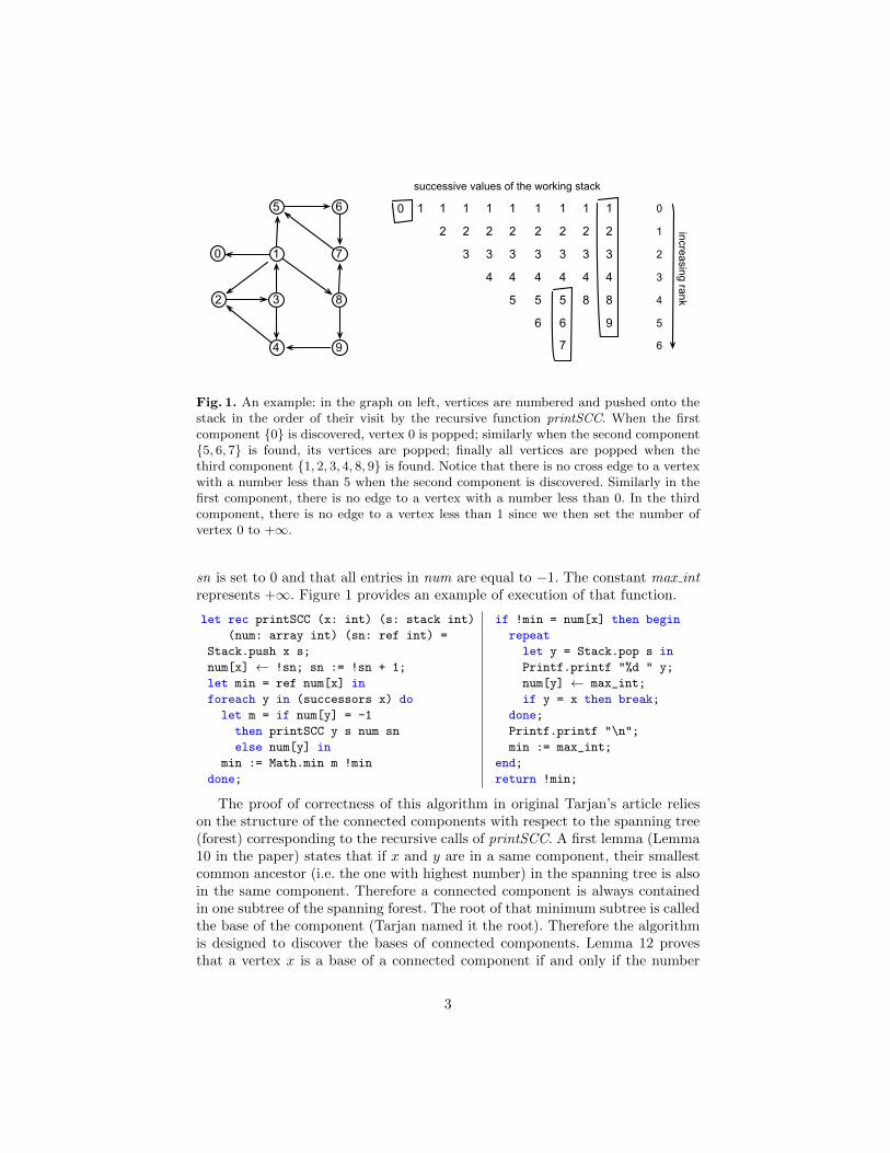
Tarjan-1972 algorithm [26, 1, 24] for finding (strongly) connected componentsin a directed graph performs a single depth-first search traversal. It maintains astack of visited vertices and a numbering of vertices. Initially the stack is emptyand the serial number of all vertices is −1. Then vertices get increasing serialnumbers in the order of their visit. Each vertex is visited once. The search isrealized by a recursive function which starts from any unvisited vertex x, pushesit on the stack, visits the directly reachable vertices from x, and returns theminimum value of the numbers of all vertices accessible from x by at most onecross-edge. A cross-edge is an edge between an unvisited vertex and an alreadyvisited vertex. If there is no such edge, the returned value is +∞. When thereturned value is equal to the number of x, a new component cc containing xis found and all vertices of cc are then at top of the stack, x being the low-est. Therefore the stack is popped until x and the numbers of the componentmembers are set to +∞, which withdraws them from further calculations in thefollowing visits of vertices.

To make this algorithm more explicit, we consider the below recursive func-tion printSCC which prints the connected components reachable from any givenvertex x and returns an integer. It works with a given stack s, an array num ofnumbers, and a current serial number sn. The program written in two columnsadopts a syntax close to the one of (Why3-)ML. The set of vertices directlyreachable from vertex x by a single edge is represented by the set (successorsx). This set can be implemented by a list of integers. We suppose that initially

2

1 1 1 1 1

2 2 2 2

3 3 3

4 4

5

1

2

3

4

5

6

1 1

2 2

3 3

4 4

8 8

1

2

3

4

5

6 9

7

successive values of the working stack

0

1

2

3

4

5

6

increasing rank2 83

4 9

1 7

5 6

0

0

Fig. 1. An example: in the graph on left, vertices are numbered and pushed onto thestack in the order of their visit by the recursive function printSCC. When the firstcomponent {0} is discovered, vertex 0 is popped; similarly when the second component{5, 6, 7} is found, its vertices are popped; finally all vertices are popped when thethird component {1, 2, 3, 4, 8, 9} is found. Notice that there is no cross edge to a vertexwith a number less than 5 when the second component is discovered. Similarly in thefirst component, there is no edge to a vertex with a number less than 0. In the thirdcomponent, there is no edge to a vertex less than 1 since we then set the number ofvertex 0 to +∞.

sn is set to 0 and that all entries in num are equal to −1. The constant max intrepresents +∞. Figure 1 provides an example of execution of that function.

let rec printSCC (x: int) (s: stack int)

(num: array int) (sn: ref int) =

Stack.push x s;

num[x] ← !sn; sn := !sn + 1;

let min = ref num[x] in

foreach y in (successors x) do

let m = if num[y] = -1

then printSCC y s num sn

else num[y] in

min := Math.min m !min

done;

if !min = num[x] then begin

repeat

let y = Stack.pop s in

Printf.printf "%d " y;

num[y] ← max_int;

if y = x then break;

done;

Printf.printf "\n";

min := max_int;

end;

return !min;

The proof of correctness of this algorithm in original Tarjan’s article relieson the structure of the connected components with respect to the spanning tree(forest) corresponding to the recursive calls of printSCC. A first lemma (Lemma10 in the paper) states that if x and y are in a same component, their smallestcommon ancestor (i.e. the one with highest number) in the spanning tree is alsoin the same component. Therefore a connected component is always containedin one subtree of the spanning forest. The root of that minimum subtree is calledthe base of the component (Tarjan named it the root). Therefore the algorithmis designed to discover the bases of connected components. Lemma 12 provesthat a vertex x is a base of a connected component if and only if the number

3

Fig. 2. Spanning forest: LOWLINK(x) is 0, 1, 1, 1, 2, 5, 5, 5, 4, 4 for 0 ≤ x ≤ 9

of x is equal to the value of so-called LOWLINK(x), which corresponds to thevalue computed by printSCC with x as input.

LOWLINK(x) = min ( {num[x]} ∪ {num[y] | x ∗=⇒ z ↪→ y

∧ x and y are in the same connected component} )

where x∗

=⇒ z means that z is a descendant of x in the spanning forest andz ↪→ y means that there is a cross-edge from z to y (that is either an edge toan ancestor y of x, or to a cousin y of x, or to a descendant y of a child of x).Notice that in the second case, cousin y could only be at left of x in the spanningtree. The trick of the algorithm is that the LOWLINK function can be simplycalculated through a single depth-first-search.

The proof of that Lemma 12 is about spanning trees and not about therecursive function which implements the depth-first-search. In order to make aformal proof of the algorithm, we may either formalize spanning trees and extracta program from these formal specifications, or directly manipulate the programand adapt the previous abstract proof to the various steps of this program. Weprefer the latter alternative which is more speaking to a programmer and maybeeasier to understand.

Our program will be expressed in a functional programming style. Thus weavoid side-effects and mutable variables. This Why3-ML program is based on twomutually recursive functions dfs1 and dfs which respectively take as argumentsa vertex x and a set of vertices roots, and which return the number n of theoldest vertex accessible by at most one cross-edge. Both functions work with anenvironment represented by a record with four fields: stack for the working stack,sccs for the set of already computed connected components, sn for the currentavailable serial number and num for the numbering mapping. The environmentat end of both functions is also returned in their results. Thus the result of dfs1and dfs is a pair (n, e′) where n is the number of the oldest vertex accessible

4

by at most one cross-edge and e’ is the environment at end of these functions.The main program tarjan calls dfs with all vertices as roots and an emptyenvironment, i.e. an empty stack, an empty set of connected components, a nullserial number and a constant mapping of vertices to −1.

let rec dfs1 x e =

let n = e.sn in

let (n1, e1) = dfs (successors x) (add_stack_incr x e) in

let (s2, s3) = split x e1.stack in

if n1 < n then (n1, e1) else

(max_int(), {stack = s3; sccs = add (elements s2) e1.sccs;

sn = e1.sn; num = set_max_int s2 e1.num})

with dfs roots e = if is_empty roots then (max_int(), e) else

let x = choose roots in

let roots’ = remove x roots in

let (n1, e1) = if e.num[x] 6= -1 then (e.num[x], e) else dfs1 x e in

let (n2, e2) = dfs roots’ e1 in (min n1 n2, e2)

let tarjan () =

let e0 = {stack = Nil; sccs = empty; sn = 0; num = const (-1)} in

let (_, e’) = dfs vertices e0 in e’.sccs

The data structures used by these functions are the ones of the Why3 stan-dard library. For lists we have the constructors Nil, Cons and the function el-ements which returns the set of elements of a list. For finite sets, we have theempty set empty, and functions add to add an element to a set, remove to re-move an element from a set, choose to pick an element in a set, and cardinal,is empty with intuitive meanings. We also use maps (instead of mutable arrays)with functions const denoting the constant function, [] to get the value of anelement and [←] to create a new map with an element set to a given value.Thus we can define an abstract type vertex for vertices and a constant verticesfor the finite set of all vertices in the graph. The type env of environments is arecord with the four fields stack, sccs, sn and num whose meanings were statedabove.

type vertex

constant vertices: set vertex

function successors vertex : set vertex

function max_int (): int = cardinal vertices

type env = {stack: list vertex; sccs: set (set vertex);

sn: int; num: map vertex int}

Finally the function dfs1 uses the following three functions. Two of themhandle environments: add stack incr pushes a vertex on the stack and sets itsnumber to the value of the current serial number which is then incremented,set max int sets all the elements of a stack to max int(). The polymorphic func-tion split returns the pair of sublists produced by decomposing a list with respectto the first occurrence of an element.

let add_stack_incr x e = let n = e.sn in

5

{stack = Cons x e.stack; sccs = e.sccs; sn = n+1; num = e.num[x ← n]}

let rec set_max_int (s : list vertex)(f : map vertex int) =

match s with

| Nil → f

| Cons x s’ → (set_max_int s’ f)[x ← max_int()]

end

let rec split (x : α) (s: list α) : (list α, list α) =

match s with

| Nil → (Nil, Nil)

| Cons y s’ → if x = y then (Cons x Nil, s’) else

let (s1’, s2) = split x s’ in ((Cons y s1’), s2)

end

We will assume that the imperative program printSCC behaves as the func-tions dfs1 and dfs. Our formal proof will only work on these two functions.We experimented several formal proofs of imperative versions, but they alwayslooked over-complex (that complexity is mainly notational, since one alwayshas to refer to the value of a variable at a given point of the program). To beconvinced that the functions dfs1 and dfs follow the algorithm in the originalpaper, we notice that instead of printing the connected components, we accu-mulate them in the sccs field of environments and produce them as the resultof the main function tarjan. We also use dfs to recursively execute the iterativeloop of printSCC. The heart of the algorithm is in the body of function dfs1where we split the working stack with respect to the vertex x giving two lists s2and s3 (the last element of s2 is x ). Then we test if the elements of s2 forms anew connected component. In fact this test could be done before splitting, butthe formal proof looks clearer if we keep them in that order.

Notice a small modification between our presentation and the one of theoriginal version. In dfs1, we test n1 < n instead of n1 6= n. In the imperativeprogram, the minimum is initialized to the number of x. Thus this initial valueis used for two distinct purposes: the case when x is the root of a new connectedcomponent and the case when x is the top of the working stack. In the lattercase we prefer returning +∞ for dfs which corresponds to the simpler formula E .

LOWLINK(x) = min {num[y] | x ∗=⇒ z ↪→ y (E)

∧ x and y are in the same connected component}

A final remark is that we could have inlined dfs1 in dfs or transformed thecall to dfs1 into a call to dfs with a singleton set of roots as argument. Bothalternatives do not simplify the proof, nor the invariants. Altogether we feel ourpresentation easier to read.

3 Invariants

This algorithm collects connected components in the sccs field of environmentsand we have to maintain that property along the execution of the program.

6

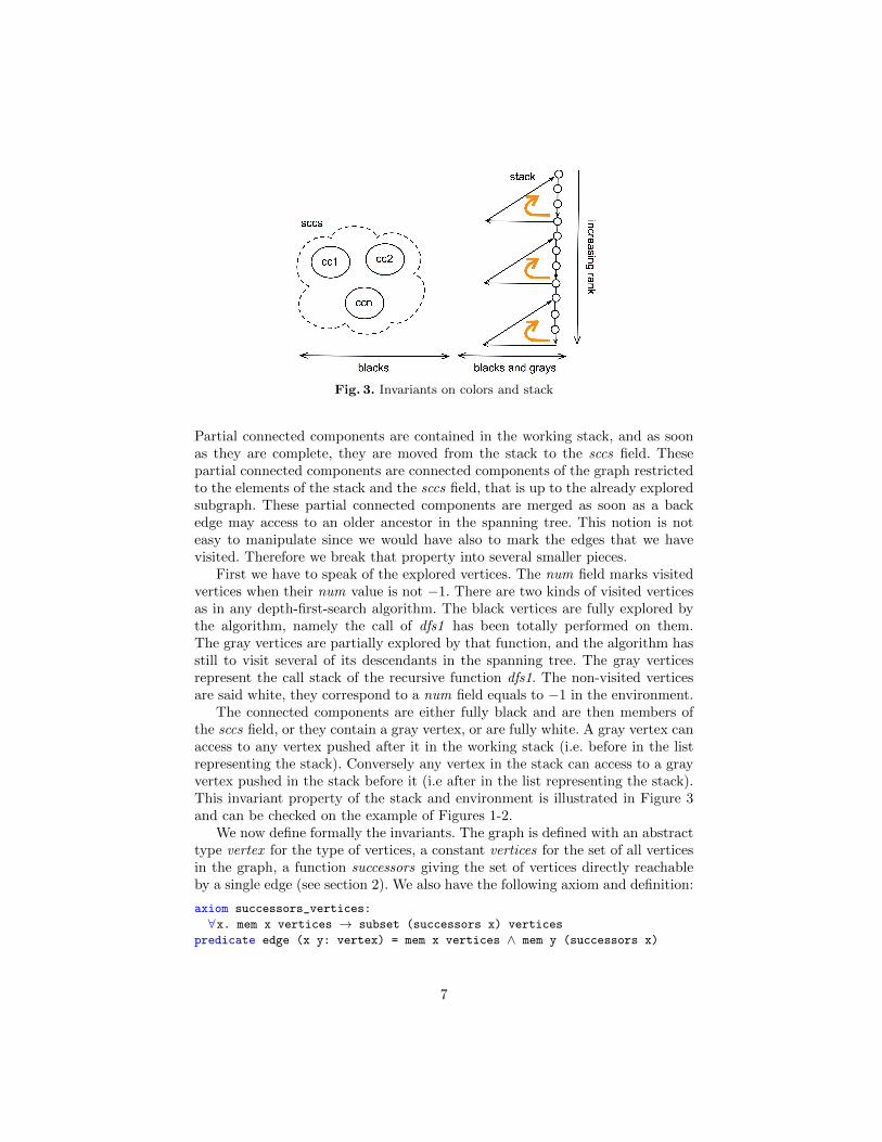
Fig. 3. Invariants on colors and stack

Partial connected components are contained in the working stack, and as soonas they are complete, they are moved from the stack to the sccs field. Thesepartial connected components are connected components of the graph restrictedto the elements of the stack and the sccs field, that is up to the already exploredsubgraph. These partial connected components are merged as soon as a backedge may access to an older ancestor in the spanning tree. This notion is noteasy to manipulate since we would have also to mark the edges that we havevisited. Therefore we break that property into several smaller pieces.

First we have to speak of the explored vertices. The num field marks visitedvertices when their num value is not −1. There are two kinds of visited verticesas in any depth-first-search algorithm. The black vertices are fully explored bythe algorithm, namely the call of dfs1 has been totally performed on them.The gray vertices are partially explored by that function, and the algorithm hasstill to visit several of its descendants in the spanning tree. The gray verticesrepresent the call stack of the recursive function dfs1. The non-visited verticesare said white, they correspond to a num field equals to −1 in the environment.

The connected components are either fully black and are then members ofthe sccs field, or they contain a gray vertex, or are fully white. A gray vertex canaccess to any vertex pushed after it in the working stack (i.e. before in the listrepresenting the stack). Conversely any vertex in the stack can access to a grayvertex pushed in the stack before it (i.e after in the list representing the stack).This invariant property of the stack and environment is illustrated in Figure 3and can be checked on the example of Figures 1-2.

We now define formally the invariants. The graph is defined with an abstracttype vertex for the type of vertices, a constant vertices for the set of all verticesin the graph, a function successors giving the set of vertices directly reachableby a single edge (see section 2). We also have the following axiom and definition:

axiom successors_vertices:

∀x. mem x vertices → subset (successors x) vertices

predicate edge (x y: vertex) = mem x vertices ∧ mem y (successors x)

7

where mem and subset are the predicates denoting the membership in a setand the subset relation between two sets. Therefore edge is the binary relationdefining the graph. The Why3 standard library defines paths in graphs as aninductive predicate and we also use a reachability predicate:

inductive path vertex (list vertex) vertex =

| Path_empty: ∀x: vertex. path x Nil x

| Path_cons: ∀x y z: vertex, l: list vertex.

edge x y → path y l z → path x (Cons x l) z

predicate reachable (x y: vertex) = ∃l. path x l y

Strongly connected components are naturally defined as non-empty maximalsets of vertices connected in both ways by paths.

predicate in_same_scc (x y: vertex) = reachable x y ∧ reachable y x

predicate is_subscc (s: set vertex) =

∀x y. mem x s → mem y s → in_same_scc x y

predicate is_scc (s: set vertex) = not is_empty s ∧is_subscc s ∧ (∀s’. subset s s’ → is_subscc s’ → s == s’)

The colors of vertices are defined by membership to two sets: blacks and graysfor the set of black and gray vertices. A white vertex is neither in blacks, nor ingrays. (The grays set can also be implicit, since gray vertices are the non-blackelements of the working stack, but we feel simpler to keep it explicit). These twosets blacks and grays are ghost variables for the Why3-ML program. They areused inside the logic of the proof, but they affect neither the control flow, northe result of the program. We will treat them differently since blacks will be anew ghost field in environments and grays will be an extra ghost argument tothe functions dfs1, dfs and tarjan. Adding the gray set as another new field ofenvironments was intractable in the proof. We will discuss that point later. Thusthe new type of environments is as follows:

type env = {ghost blacks: set vertex; stack: list vertex;

sccs: set (set vertex); sn: int; num: map vertex int}

and the main invariant (I) of our program will be: (I)

wf_env e grays ∧ ∀cc. mem cc e.sccs ↔ subset cc e.blacks ∧ is_scc cc

where wf env defines a well formed environment and the other conjunct specifiesthat the black connected components are exactly the elements of the sccs field.

The definition of a well formed environment is done in three steps. First wedefine a well formed coloring: the grays and blacks sets are disjoint subsets ofvertices in the graph; the elements of the stack is the union of grays and thedifference of blacks and the union of elements of sccs; the elements of sccs areall black. The operations union, inter, diff on sets are defined in the Why3standard library. But we had to define the big union set of axiomatically.

predicate wf_color (e: env) (grays: set vertex) =

let {stack = s; blacks = b; sccs = ccs} = e in

subset (union grays b) vertices ∧ inter b grays == empty ∧

8

elements s == union grays (diff b (set_of ccs)) ∧subset (set_of ccs) b

In the next two steps, we use two new predicates and a new definition. Theno black to white predicate states that there is no edge from a black vertex toa white vertex. Any depth-first search respects that property since the blackset is saturated by reachability. The simplelist predicate says that a list has norepetitions i.e. there is no more than one occurrence of any element. Our workingstack satisfies that predicate since any vertex is visited no more than once. (Thenum occ function belongs to the Why3 standard library)

predicate no_black_to_white (blacks grays: set vertex) =

∀x x’. edge x x’ → mem x blacks → mem x’ (union blacks grays)

predicate simplelist (l: list α) = ∀x. num_occ x l ≤ 1

The rank function gives the position of an element in a list starting from theend of the list. In a working stack of length `, the ranks of the bottom and topof the stack are 0 and ` − 1 (see Figures 1 and 3). The rank function allows toorder vertices in the stack with respect to their positions. It could be done justwith numbers of the vertices, but we shall discuss that point later. (lmem andlength are the Why3 functions for membership in and length of a list)

function rank (x: α) (s: list α): int =

match s with

| Nil → max_int()

| Cons y s’ → if x = y && not (lmem x s’) then length s’ else rank x s’

end

The well formed numbering is a bit long to state formally, but is quite easy tounderstand. Numbers of vertices can be −1, non-negative or +∞ (i.e. max int()).Finite numbers range between −1 and sn (excluded). The serial number sn isthe number of non-white vertices. A vertex has number +∞ if and only if it is inthe set of already discovered connected components. It has number −1 exactlywhen it is a white vertex. Finally numbers of vertices in the stack are orderedas their ranks.

A well-formed environment is well colored, well numbered, respects the non-black-to-white property, contains a stack without repetitions and the partialconnected components property described above. Thus there should be a pathbetween any gray vertex and any higher-ranked vertex in the stack, and con-versely any vertex in the stack can reach a lower-ranked gray vertex (see Fig-ure 3).

predicate wf_num (e: env) (grays: set vertex) =

let {stack = s; blacks = b; sccs = ccs; sn = n; num = f} = e in

(∀x. -1 ≤ f[x] < n ≤ max_int() ∨ f[x] = max_int()) ∧n = cardinal (union grays b) ∧(∀x. f[x] = max_int() ↔ mem x (set_of ccs)) ∧(∀x. f[x] = -1 ↔ not mem x (union grays b)) ∧(∀x y. lmem x s → lmem y s → f[x] < f[y] ↔ rank x s < rank y s)

9

predicate wf_env (e: env) (grays: set vertex) = let s = e.stack in

wf_color e grays ∧ wf_num e grays ∧no_black_to_white e.blacks grays ∧ simplelist s ∧(∀x y. mem x grays → lmem y s → rank x s ≤ rank y s → reachable x y)

∧(∀y. lmem y s → ∃x. mem x grays ∧ rank x s ≤ rank y s ∧ reachable y x)

4 Pre-/Post-conditions

The previous invariant (I) of Section 3 is surely a pre-condition and a post-condition of the dfs1 and dfs functions. We have several simple extra pre-conditions, namely the argument x of dfs1 should be a white vertex and allgray vertices must reach x. Similarly for dfs, the vertices in roots can all beaccessed by all gray vertices.

The post-conditions are more subtle. The simplest one is the monotony prop-erty subenv which relates the environments at the beginning and at the end ofthe function. It states that the working stack is extended by a new black area,that the black set of vertices and the set of discovered connected components areaugmented, and that the numbers of vertices in the initial stack are unchanged.Vertices whose numbers change are either the new white vertices pushed ontothe stack or the vertices moved to the sccs field; in the latter case they do notbelong to the initial stack. (++ is the infix append operator)

predicate subenv (e e’: env) =

(∃s. e’.stack = s ++ e.stack ∧ subset (elements s) e’.blacks) ∧subset e.blacks e’.blacks ∧ subset e.sccs e’.sccs ∧(∀x. lmem x e.stack → e.num[x] = e’.num[x])

There are four main post-conditions. For dfs1, the last one P4 tells that thewhite vertex x argument of dfs1 is blackened at the end of the function. Theother post-conditions give properties of the number n returned in the resultingpair. One way of specifying n is to give its definition by equation (E) of Section 2.Then we would have to handle white paths which are not easy to handle. Insteadof paths we will only consider edges with the following three post-conditionswhich describe implicit properties of the result n. Post-condition P1 says that ncannot be greater than the number of x. Then n is either +∞ and then x is alsonumbered +∞, or n is the number of some vertex in the stack reachable from x(post-condition P2). Thirdly if an edge starts from the new part of the resultingstack to a vertex y in the old stack, then n is smaller than the number of thaty (post-condition P3). For dfs, all roots are either black or gray at the end ofthe function (post-condition P ′1). The other post-conditions P ′2, P ′3, P ′4 are thenatural extension to sets of the post-conditions of dfs1. These post-conditionsuse the following predicates.

predicate num_reachable (n: int) (x: vertex) (e: env) =

∃y. lmem y e.stack ∧ n = e.num[y] ∧ reachable x y

10

predicate xedge_to (s1 s3: list vertex) (y: vertex) =

(∃s2. s1 = s2 ++ s3 ∧ ∃x. lmem x s2 ∧ edge x y) ∧ lmem y s3

predicate access_to (s: set vertex) (y: vertex) =

∀x. mem x s → reachable x y

The function dfs1 can now be written as follows.

let rec dfs1 x e (ghost grays) =

requires{mem x vertices}

requires{access_to grays x}

requires{not mem x (union e.blacks grays)}

(* invariants *)

requires{wf_env e grays}

requires{∀cc. mem cc e.sccs ↔ subset cc e.blacks ∧ is_scc cc}

returns{(_, e’) → wf_env e’ grays}

returns{(_, e’) → ∀cc. mem cc e’.sccs ↔ subset cc e’.blacks ∧ is_scc cc}

(* post-conditions *)

returns{(n, e’) → n ≤ e’.num[x]} (*P1*)

returns{(n, e’) → n = max_int() ∨ num_reachable n x e’} (*P2*)

returns{(n, e’) → ∀y. xedge_to e’.stack e.stack y → n ≤ e’.num[y]} (*P3*)

returns{(_, e’) → mem x e’.blacks} (*P4*)

(* monotony *)

returns{(_, e’) → subenv e e’}

let n = e.sn in

let (n1, e1) = dfs (successors x) (add_stack_incr x e) (add x grays) in

let (s2, s3) = split x e1.stack in

if n1 < n then (n1, add_blacks x e1) else

(max_int(), {blacks = add x e1.blacks; stack = s3;

sccs = add (elements s2) e1.sccs; sn = e1.sn;

num = set_max_int s2 e1.num})

(The keywords “requires” and “returns” represent pre- and post-conditions; “re-turns” allows pattern matching on the result). The functions dfs and tarjan havesimilar pre-/post-conditions.

with dfs roots e (ghost grays) =

requires{subset roots vertices}

requires{∀x. mem x roots → access_to grays x}

(* invariants *)

requires{wf_env e grays}

requires{∀cc. mem cc e.sccs ↔ subset cc e.blacks ∧ is_scc cc}

returns{(_, e’) → wf_env e’ grays}

returns{(_, e’) → ∀cc. mem cc e’.sccs ↔ subset cc e’.blacks ∧ is_scc cc}

(* post-conditions *)

returns{(n, e’) → ∀x. mem x roots → n ≤ e’.num[x]}

returns{(n, e’) → n = max_int() ∨ ∃x. mem x roots ∧ num_reachable n x e’}

returns{(n, e’) → ∀y. xedge_to e’.stack e.stack y → n ≤ e’.num[y]}

returns{(_, e’) → subset roots (union e’.blacks grays)}

(* monotony *)

returns{(_, e’) → subenv e e’}

11

if is_empty roots then (max_int(), e) else

let x = choose roots in

let roots’ = remove x roots in

let (n1, e1) = if e.num[x] 6= -1 then (e.num[x], e)

else dfs1 x e grays in

let (n2, e2) = dfs roots’ e1 grays in (min n1 n2, e2)

let tarjan () =

returns{r → ∀cc. mem cc r ↔ subset cc vertices ∧ is_scc cc}

let e0 = {blacks = empty; stack = Nil; sccs = empty;

sn = 0; num = const (-1)} in

let (_, e’) = dfs vertices e0 empty in e’.sccs

5 The formal proof

The proof of these post-conditions relies on three main remarks inside dfs1. Inthe function dfs, proofs are more routine and could be treated automatically.

First as we already discussed about partial connected components, it is clearthat when the stack e1.stack is split into two pieces s2 and s3 with x as the lastelement in s2, the elements of s2 form a subset of a connected component. Anyvertex y in s2 has higher rank than x and since x is gray in the call of dfs onthe successors of x, invariant (I) at end of dfs says that x reaches y. Conversely,we remark that the extension of the stack s3 appended with x is black by themonotony condition at end of dfs. Therefore the elements of s2 are either blackor x. So invariant (I) at end of dfs says that vertex y in s2 can reach a grayvertex z of lower rank, since s2 only contains black vertices and x, the rank ofz is smaller than or equal to the rank of x. Therefore again by invariant (I) atend of dfs, there is a path from z to x. Hence any element of s2 is connectedboth ways to x and therefore the elements of s2 form a subset of a connectedcomponent.

In dfs1, in case we have n1 < n, we prove that there is a gray vertex inthe connected component of x (i.e. the same component as all elements in s2).Therefore the connected component is not fully black and it cannot be insertedin the sccs field of the environment. By post-condition P ′2 of dfs, we know thanx can reach a vertex y in the stack with number n1 (n1 cannot be +∞ sincen1 < n = e.sn ≤ +∞). We also have by the monotony condition in dfs:

e1.num[y] = n1 < n = e.sn

= (add_stack_incr x e}).num[x]

= e1.num[x]

By invariant (I), the vertex y has a strictly smaller rank than x. Again by (I),the vertex y can reach a gray vertex z with rank lower than y in the stack at endof dfs. Therefore x can reach z gray with lower rank. Thus z can also reach x byinvariant (I). We indeed proved there is a gray vertex z in the same connectedcomponent as x.

In dfs1, in case we have n1 ≥ n, we prove that s2 is the connected componentof x. Let us consider a vertex y in the same connected component as x. We show

12

that y belongs to s2. We proceed by contradiction. Suppose y is not in s2. Sincethere is a path from x in s2 to y not in s2, there is an edge from x′ to y′ on thatpath such that x′ is in s2 and y′ is not in s2. Moreover x′ and y′ are in the samecomponent as x. We have three subcases:

– y′ is in the set union of all members of sccs. This means that x is also inthat big union. Therefore x would be black. Impossible since x is white.

– y′ is in the working stack e1.stack but not in the s2 part. Therefore y′ isin s3 (the other part of the split) and has rank strictly lower than the oneof x. By (I) at end of dfs, we have that the number of y′ is strictly lessthan the number of x. Then there are two cases. When x′ is x, Then y′ is asuccessor of x. Post-condition P ′1 states that n1 is smaller than the numberof y′. Then n1 < n. Impossible. When x′ is not x, the vertex x′ is not thelast element of s2 and the edge from x′ to y′ crosses the border between thestacks e1.stack and Cons x s3, which are the stacks at end and beginning ofdfs. Hence n1 is less than the number of y′ in e1 by post-condition P ′3. Thusn1 < n. Impossible.

– y′ is white. When x′ = x, then y′ is in the successors of x. It cannot be whiteby post-condition P ′4. When x′ is not x, vertex x′ is in the black extension ofthe stack at end of dfs. Therefore x′ is black. This is impossible since thereis no edge from a black vertex to a white vertex.

Thus the elements of s2 form a complete connected component. At end of dfs1,the vertex x is turned to black and therefore the component can be inserted inthe field sccs of the current environment.

The three main above remarks are implemented in the Why3-ML programby adding intermediate assertions in the body of dfs1. Namely the body is now:

let n = e.sn in

let (n1, e1) = dfs (successors x) (add_stack_incr x e) (add x grays) in

let (s2, s3) = split x e1.stack in

assert{is_last x s2 ∧ s3 = e.stack ∧subset (elements s2) (add x e1.blacks)};

assert{is_subscc (elements s2)};

if n1 < n then begin

assert{∃y. mem y grays ∧ lmem y e1.stack ∧ e1.num[y] < e1.num[x] ∧reachable x y};

(n1, add_blacks x e1) end

else begin

assert{∀y. in_same_scc y x → lmem y s2};

assert{is_scc (elements s2)};

assert{inter grays (elements s2) = empty};

(max_int(), {blacks = add x e1.blacks; stack = s3;

sccs = add (elements s2) e1.sccs; sn = e1.sn;

num = set_max_int s2 e1.num}) end

where the polymorphic predicate is last is defined by:

predicate is_last (x: α) (s: list α) = ∃s’. s = s’ ++ Cons x Nil

13

These assertions are proved automatically except for the third and the fourthones manually proved in Coq along the lines of the second and the third remarksexplained above. All pre-conditions and post-conditions are automatically proved(see Table 1 or the detailed session at [9]). These Coq proofs use the compactssreflect syntax, several lemmas proved in Why3 and are 65+168 line-long. Thebody of the functions dfs and tarjan is unchanged except for two assertionswhich ease the behaviour of the automatic provers. In dfs, one adds

assert{e.num[x] 6= -1 ↔ (lmem x e.stack ∨ mem x e.blacks)};

before the −1 test for the number of x. In tarjan we add this assertion

assert{subset vertices e’.blacks};

which ensures the blackness of all vertices before returning the result. Noticefinally the sixth assertion in dfs1 which caused us many problems and eases theautomatic proof of properties about sets.

There is no space here to fully describe the lemmas that we added in ourproof. We have 8 lemmas about ranks in lists, 4 about simple lists, 12 aboutsets, 3 about sets of sets, 2 about paths, 5 about connected components, 4special ones to show proof obligations. We present three typical lemmas. Thefirst one states that when the vertex x is in the list s, the rank of x in s isinvariant by the extension of s.

lemma rank_app_r:

∀x:α, s s’. lmem x s → rank x s = rank x (s’ ++ s)

The second lemma shows that when a path l joins x to y and the vertex xis in a set s and the vertex y is not in s, then there is an edge from vertex x′

in s to vertex y′ not in s such that x reaches x′ and y′ reaches y. In fact x′ andy′ are on that path l. This lemma is critical to reduce properties on paths toproperties on edges.

lemma xset_path_xedge:

∀x y l s. mem x s → not mem y s → path x l y →∃x’ y’. mem x’ s ∧ not mem y’ s ∧ edge x’ y’ ∧

reachable x x’ ∧ reachable y’ y

The third lemma is used in the second assertion in the body of dfs1. Thestatement is not interesting by itself and this lemma is part of the four specializedlemmas. It shows the use of the by logical connector in Why3 [11]. This operatoris no more than an explicit cut-rule meaning that in order to prove A withA by B, one can prove B and B → A in current environment.

lemma subscc_after_last_gray:

∀x e g s2 s3. wf_env e (add x g) →let {blacks = b; stack = s} = e in

s = s2 ++ s3 → is_last x s2 →subset (elements s2) (add x b) → is_subscc (elements s2)

by (access_to (add x g) x

by inter (add x g) (elements s2) == add x empty)

∧ access_from x (elements s2)

14

provers Alt- CVC3 CVC4 Coq E- Spass Yices Z3 all #VC #POErgo prover

38 lemmas 2.35 0.23 5.79 0.66 0.75 0.21 9.99 77 38split 0.09 0.2 0.29 6 6add stack incr 0.01 0.01 1 1add blacks 0.01 0.01 1 1set max int 0.02 0.02 1 1dfs1 53.52 12.88 36.39 3.06 28.06 9.01 142.92 218 24dfs 4.6 0.23 11.63 0.31 16.77 51 35tarjan 0.44 0.44 16 6

total 61.04 13.54 53.81 3.06 28.72 0.75 0.21 9.32 170.45 371 112

Table 1. These are the provers results in seconds on a 3.3 GHz Intel Core i5 proces-sor. The two last columns contains the numbers of verification conditions and proofobligations. Notice that there could be several VCs per proof obligation.

6 Conclusion

We presented a formal proof of Tarjan’s algorithm for computing strongly con-nected components in a graph. There are other (less efficient) algorithms. Wedid prove the two-passes Kosaraju’s algorithm in a similar way, but the prooffor Tarjan is more involved. Many of the lemmas in our proof can be used forother algorithms on graphs such as acyclicity test, articulation points, or bicon-nected components. We had to fight with properties on sets, maybe because ofa misusage of the Why3 library and the distinction between == (membership inboth directions) and the extensional equality =.

In our presentation, we treated differently the blacks and grays sets. Themain reason is that the automatic provers have difficulties when the data is toostructured. We indeed started with flat formalizations where environment fieldswere passed as arguments of the functions. Then the automatic provers workedsplendidly. But the presentation was uglier [10]. As soon as you have structuressuch as records, the automatic proofs are more complex and we had to help themwith the inlining strategies of the Why3 ide. At time of writing this article, wecould not succeed in introducing the grays set in the environment.

We also use the rank function and it is unclear if reasoning with the numfield could be sufficient. Indeed if you want to escape painful properties aboutspanning trees and white paths, you have to speak about positions in the workingstack. The ranks are an explicit expression of these positions. Moreover we hadversions of Tarjan algorithm with just ranks and no numbers. The properties arethen simpler, since there are less many variables in the algorithm: stack, blacks,grays, sccs and functions return ranks. But we experienced that the presentationis further from the initial sequential algorithm and therefore was less convincing.

We also said that white paths are difficult to handle and we then took animplicit description of the results of functions dfs1 and dfs. One of the reasons

15

is that a white path is a volatile notion, since its color could be modified on itsintermediate vertices. The proofs are indeed longer than with simple edges.

Notice also that we only prove partial correctness. Total correctness is veryeasy since a variant with lexicographic ordering on the pair made of the numberof white vertices and the number of roots is clearly decreasing.

This comes to the comparison with other formalisms. We have a similar prooffully in Coq/ssreflect [12] with the Mathematical Components library. The proofis 920-line long and a version with explicit expression of the results is 951-linelong for the version of our algorithm with just ranks and no numbers dependingupon the accounting of the Coq parts. Notice that the use of MathematicalComponents makes Coq proofs much shorter. Still our proof is between two orfour times shorter (up to the accounting of our Coq proofs), and we think thatour proof is also much more readable. Coq demanded some agility to follow thesame partial correctness proof. It would also be interesting to redo our proofin Isabelle or another system. In the literature, many articles are about graphconcurrent algorithms, either embedded in Coq [25] or in separation logic [17, 23]or both. None of them treat strong connectivity except [22] by Kosaraju methodand with reasoning more on spanning trees than on the effective program.

Hence, for a non-obvious algorithm, Why3 allowed us to achieve a not toolong formal proof, not much sophisticated, as simple-minded as first-order logic,and fully described in this article. The system is easy to use, but very unstablewhich makes uneasy incremental development, although the replay function [4]of the Why3 ide greatly helps. But we gained in readability, which seems to usa very important criterion in formal proofs of programs. Thus we were able topresent here the full details of this formal proof.

Acknowledgments

Thanks to the Why3 group at Inria-Saclay/LRI-Orsay for very valuable advices,to Cyril Cohen and Laurent Thery for their fantastic expertise in Coq proofs, toClaude Marche and the reviewers for many corrections.

References

1. Aho, A.V., Hopcroft, J.E., Ullman, J.D.: The Design and Analysis of ComputerAlgorithms. Addison-Wesley (1974)

2. Appel, A.W.: Verified Functional Algorithms. www.cs.princeton.edu/~appel/

vfa/ (August 2016)3. Bobot, F., Filliatre, J.C., Marche, C., Melquiond, G., Paskevich, A.: The Why3

platform, version 0.86.1. LRI, CNRS & Univ. Paris-Sud & INRIA Saclay, version0.86.1 edn. (May 2015), why3.lri.fr/download/manual-0.86.1.pdf

4. Bobot, F., Filliatre, J.C., Marche, C., Melquiond, G., Paskevich, A.: PreservingUser Proofs Across Specification Changes. In: Cohen, E., Rybalchenko, A. (eds.)Fifth Working Conference on Verified Software: Theories, Tools and Experiments.vol. 8164, pp. 191–201. Springer, Atherton, United States (May 2013), hal.inria.fr/hal-00875395

16

5. Bobot, F., Filliatre, J.C., Marche, C., Paskevich, A.: Let’s Verify This with Why3.Software Tools for Technology Transfer (STTT) 17(6), 709–727 (2015), hal.inria.fr/hal-00967132

6. Chargueraud, A.: Program verification through characteristic formulae. In: Hu-dak, P., Weirich, S. (eds.) Proceeding of the 15th ACM SIGPLAN interna-tional conference on Functional programming (ICFP). pp. 321–332. ACM (2010),arthur.chargueraud.org/research/2010/cfml

7. Chargueraud, A.: Higher-order representation predicates in separation logic. In:Proceedings of the 5th ACM SIGPLAN Conference on Certified Programs andProofs. pp. 3–14. CPP 2016, ACM, New York, NY, USA (January 2016)

8. Chargueraud, A., Pottier, F.: Machine-checked verification of the correctness andamortized complexity of an efficient union-find implementation. In: Proceedings ofthe 6th International Conference on Interactive Theorem Proving (ITP) (August2015)

9. Chen, R., Levy, J.J.: Full script of Tarjan SCC Why3 proof. Tech. rep., Iscas andInria (2017), jeanjacqueslevy.net/why3/graph/abs/scct/2/scc.html

10. Chen, R., Levy, J.J.: Une preuve formelle de l’algorithme de Tarjan-1972 pourtrouver les composantes fortement connexes dans un graphe. In: JFLA (2017)

11. Clochard, M.: Preuves taillees en biseau. In: vingt-huitiemes Journees Franco-phones des Langages Applicatifs (JFLA). Gourette, France (Jan 2017), hal.inria.fr/hal-01404935

12. Cohen, C., Thery, L.: Full script of Tarjan SCC Coq/ssreflect proof. Tech. rep.,Inria (2017), github.com/CohenCyril/tarjan

13. Coq Development Team: The coq 8.5 standard library. Tech. rep., Inria (2015),coq.inria.fr/distrib/current/stdlib

14. Filliatre, J.C., Paskevich, A.: Why3 — where programs meet provers. In: Felleisen,M., Gardner, P. (eds.) Proceedings of the 22nd European Symposium on Program-ming. Lecture Notes in Computer Science, vol. 7792, pp. 125–128. Springer (Mar2013)

15. Gonthier, G., Mahboubi, A., Tassi, E.: A Small Scale Reflection Extension forthe Coq system. Rapport de recherche RR-6455, INRIA (2008), hal.inria.fr/inria-00258384

16. Gonthier, G., et al.: Finite graphs in mathematical components (2012), ssr.

msr-inria.inria.fr/~jenkins/current/Ssreflect.fingraph.html, The full li-brary is available at www.msr-inria.fr/projects/mathematical-components-2

17. Hobor, A., Villard, J.: The ramifications of sharing in data structures. In: Pro-ceedings of the 40th Annual ACM SIGPLAN-SIGACT Symposium on Principlesof Programming Languages. pp. 523–536. POPL ’13, ACM, New York, NY, USA(2013), doi.acm.org/10.1145/2429069.2429131

18. Lammich, P., Neumann, R.: A framework for verifying depth-first search algo-rithms. In: Proceedings of the 2015 Conference on Certified Programs and Proofs.pp. 137–146. CPP ’15, ACM, New York, NY, USA (2015), doi.acm.org/10.1145/2676724.2693165

19. Levy, J.J.: Essays for the Luca Cardelli Fest, chap. Simple proofs of simple pro-grams in Why3. Microsoft Research Cambridge, MSR-TR-2014-104 (2014)

20. Mehta, F., Nipkow, T.: Proving pointer programs in higher-order logic. In: CADE(2003)

21. Poskitt, C.M., Plump, D.: Hoare logic for graph programs. In: VSTTE (2010)22. Pottier, F.: Depth-first search and strong connectivity in Coq. In: Journees Fran-

cophones des Langages Applicatifs (JFLA 2015) (Jan 2015)

17

23. Raad, A., Hobor, A., Villard, J., Gardner, P.: Verifying Concurrent Graph Al-gorithms, pp. 314–334. Springer International Publishing, Cham (2016), dx.doi.org/10.1007/978-3-319-47958-3_17

24. Sedgewick, R., Wayne, K.: Algorithms, 4th Edition. Addison-Wesley (2011)25. Sergey, I., Nanevski, A., Banerjee, A.: Mechanized verification of fine-grained con-

current programs. In: Proceedings of the 36th ACM SIGPLAN Conference onProgramming Language Design and Implementation. pp. 77–87. PLDI ’15, ACM,New York, NY, USA (2015), doi.acm.org/10.1145/2737924.2737964

26. Tarjan, R.: Depth first search and linear graph algorithms. SIAM Journal on Com-puting (1972)

27. Thery, L.: Formally-proven Kosaraju’s algorithm (2015), Inria report, Hal-01095533

28. Wengener, I.: A simplified correctness proof for a well-known algorithm comput-ing strongly connected components. Information Processing Letters 83(1), 17–19(2002)

29. Why3 Development Team: Why3 gallery of programs. Tech. rep., CNRS and Inria(2016), toccata.lri.fr/gallery

18