a segment-based speaker verification system using summit
TRANSCRIPT
A Segment-Based Speaker Verification System
Using SUMMIT
by
Sridevi Vedula Sarma
B.S., Cornell University, 1994
Submitted to the Department of Electrical Engineeringand Computer Science
in partial fulfillment of the requirements for the degree of
Master of Science in Electrical Engineering and Computer Science
at the
MASSACHUSETTS INSTITUTE OF TECHNOLOGY
April 1997
@ Massachusetts Institute of Technology 1997. All rights reserved.
A uthor ........ .................... .... ............ ...Department of Electrical Engineering
and Computer Sciencee_. Anril 9. 1Q97
Certified by........................ ,Victor W. Zue
Senior Research ScientistTJ isupervisor
.....rthur C. SmithArthur C. Smith
Accepted by.
Chairman, Departmental Committee on Graduate Students
JUL 2 4 1997 Eng.
I

A Segment-Based Speaker Verification System Using SUMMIT
bySridevi V. Sarma
Submitted to the Department of Electrical Engineering
and Computer Science
on April 20, 1997 in partial fulfillment of the
requirements for the degree of
Master of Science in Electrical Engineering and Computer Science
Abstract
This thesis describes the development of a segment-based speaker verification
system. Our investigation is motivated by past observations that speaker-specific
cues may manifest themselves differently depending on the manner of articulation
of the phonemes. By treating the speech signal as a concatenation of phone-sized
units, one may be able to capitalize on measurements for such units more readily. A
potential side benefit of such an approach is that one may be able to achieve good
performance with unit (i.e., phonetic inventory) and feature sizes that are smaller
than what would normally be required for a frame-based system, thus deriving the
benefit of reduced computation.
To carry out our investigation, we started with the segment-based speech recogni-
tion system developed in our group called SUMMIT [43], and modified it to suit our
needs. The speech signal was first transformed into a hierarchical segment network
using frame-based measurements. Next, acoustic models for each speaker were devel-
oped for a small set of six phoneme broad classes. The models represented feature
statistics with diagonal Gaussians, which characterized the principle components of
the feature set. The feature vector included averages of MFCCs, plus three prosodic
measurements: energy, fundamental frequency (FO), and duration. The size and con-
tent of the feature vector were determined through a greedy algorithm optimized on
overall speaker verification performance.
To facilitate a comparison with previously reported work [19, 2], our speaker verifi-
cation experiments were carried out using 168 speakers from the TIMIT corpus. Each
speaker-specific model was developed from the eight SI and SX sentences. Verifica-
tion was performed using the two SA sentences common to all speakers. To classify a
speaker, a Viterbi forced alignment was determined for each test utterance, and the
forced alignment score of the purported speaker was compared with those obtained
with the models of the speaker's competitors. Ideally, the purported speaker's score
should be compared to scores of every other system user. To reduce the computation,
we adopted a procedure in which the score for the purported speaker is compared
only to scores of a cohort set consisting of a small set of acoustically similar speakers.
These scores were then rank ordered and the user was accepted if his/her model's
score was within the top N scores, where N is a parameter we varied in our experi-
ments. To test for false acceptance, we used only the members of a speaker's cohort
set as impostors. We have found this method to significantly reduce computation
while minimally affecting overall performance.
We were able to achieve a performance of 0% false rejection of true users and 4.85%
false acceptance of impostors, with a simple system design. We reduced computation
significantly through the use of a small number of features representing broad-classes,
diagonal Gaussian speaker models, and using only cohort sets during testing.
Thesis Supervisor: Victor W. Zue
Title: Senior Research Scientist

Acknowledgments
The Spoken Language Systems (SLS) group provides the ideal research environment,a place where one can grow extensively both academically and emotionally. I cannoteven begin to describe how much I have learned from all members of this group. Myexperience begins with my thesis advisor Dr. Victor Zue, for whom I have the deepestrespect and gratitude. Victor not only gave me the wonderful opportunity to be apart of the SLS group, but he also provided his full support and confidence theselast 16 months. We communicated frequently with productive meetings, and I oftenfound Victor pondering over my project in his own free time along with myself. Weworked as a team and without his optimism and motivation, I may not have had thestrength to dig myself out of the bad times.
I would also like to thank my good friend Rajan Naik for all his support, love, andencouragement in my academics. He lifted my spirits up when I was down and stoodby my side unconditionally.
I also wish to thank all the other members of the Spoken Language Group for all ofthe support and friendship they have provided me. In particular I would like to thank:
Jane Chang for her time and patience in teaching me everything there is to knowabout the SLS libraries and programming languages to successfully pursue my re-search. I am deeply in debt to her and hope to help another group member half asmuch as she has helped me.
Giovanni Flammia for all his help in brushing up my skills in C and Latex and forpatiently teaching me Perl. In addition to sharing his vast background in all pro-gramming languages and the Internet, he also shared a sense of humor which oftenmade stressful times durable.
Michelle Spina for being such a good friend and colleague. She always encouraged meand guided me through rough times by sharing her experiences in academia. She alsopatiently helped me out during my learning, stages of programming in C and C++.
Mike McCandless for his patience with my pestering him with technical questionsabout how to use the recognizer and of course always having a solution to my bugs.
Ben Serridge for being a great office-mate and for giving me a beautiful bouquet offlowers after I took my oral qualifiers!
Tim Hazen for teaching me details about various methods of speech and speakerrecognition.
Ray Lau, Alex Manos, and Ray Chun for all the help they've provided and questionsthey've answered.
Jim Hugunin for introducing me to Python.
Jim Glass for acting as another supportive advisor by discussing my work, offeringgreat advice, and for relating his experiences in the field.
Lee Hetherington for his spur of the moment advice and ideas.
Stephanie Seneff for her advice about being a female at M.I.T, and of course for mak-ing me realize how much I have yet to learn!
David Goddeau, Joe Polifroni, and Christine Pao for keeping our systems up andrunning, which was a difficult task this year.
Vicky Palay and Sally Lee for everything they have done for the group and for dealingpatiently with my concerns.
I would also like to thank colleagues outside SLS who have helped me tremendouslyin adjusting to M.I.T. Babak Ayazifar taught me how to survive and succeed hereand is a reliable mentor, not to mention an excellent teacher. Likewise, I cannotthank Stark Draper enough as he was my sole partner my first semester at M.I.T. Weworked well together and I learned a great deal from him.
I would also like to acknowledge my two best childhood friends Paulina Vaca andGarrett Robbins. They make me laugh until my stomach hurts, and they allow meto escape this technical world to catch a glimpse of the world of literature and art.
Finally, I wish to thank my family for all their love and support. Without their en-couragement to succeed in life in all my endeavors, and their stress of importance forhigher education, I may not have had the strength to come this far.
This research was supported partially by NSF and DARPA.

Contents
1 Speaker Verification 11
1.1 Introduction . . . . . . . . . . . . . . . . . . . . . . . . . . . . . . . . 11
1.2 Previous Research ............................. 12
1.3 D iscussion . . . . . . . . . . . . . . . . . . . . . . . . . . . . . . . . . 15
1.4 Thesis Objective and Outline ......... ............ 16
2 System Description 18
2.1 Introduction .. ....... .. . ........ . .... .. . ... . 18
2.2 Corpus . . . . . . . . . . . . . . . . . . . . . . . . . . . . . . . . .. . 19
2.2.1 TIM IT . . . . . . . . . . . . . ... . . . . .. . . . . . . . . . 20
2.2.2 Broad Classes ........................... 20
2.3 Signal Representations .......................... 21
2.3.1 M FCCs . . . . . . . . . . . . .. . . . . . . . . . . . . . . . . 21
2.3.2 Prosodic Features ......................... 22
2.4 Segm entation ............................... 23
2.5 Measurement Search ........................... 25
2.6 Speaker M odels .............................. 27
2.7 Speaker Classification ........................... 28
2.7.1 Cohort Sets ....................... ..... 29
2.7.2 Verification Process ........................ 30
2.7.3 Scoring . . . . . . . . . . . . . . . . . . . . . . . . . . . . . . . 31
3 Experimental Results & Analysis
3.1 Overview .. .......................
3.2 Performance Measures .................
3.3 Feature Search ......... . . . ..
3.3.1 Results Using 168 Speakers ..........
3.3.2 Results Using 80 Speakers . . . . . . . ..
3.4 System Performance ..................
3.5 Performance Comparison . ...............
3.5.1 HMM Approach ....... . ....
3.5.2 Neural Network Approach . . . . . . . . . . .
3.5.3 Performance versus Computational Efficiency
4 Conclusions & Future Work
4.1 Summ ary ...... . . ......... ..........
4.2 Future W ork ....... .... .... .............
4.2.1 Robustness Issues . . . . . . . . . . . . . . . . ..
4.2.2 Exhaustive Search for Robust Features . . . . . . . . . .
4.2.3 Feature-Motivated Broad Class Selections . . . . . . . .
4.2.4 Representing Features With More Complex Distributions
4.2.5 Adaptation of Models . . . . . . . . . .
4.2.6 Incorporating into GALAXY . . . . . . . . . . . .
A Mel-frequency Cepstral Coefficients
B Linear Prediction Analysis
B.1 Estimation of Fundamental Frequency
C Feature Search Results
33
.. .. ... .. 33
. . . . . . . . 34
. . .. ... .. 34
. .. .. ... . 36
.. . . . . . . 47
. .. ... ... 50
. . . . . . . . 52
.. .. .. . 54
. . . . . . . . 55
. . . . . . . . . 55
59
.. . 59
.. . 60
. . . 60
. . . 62
. . . 62
. . . 63
. . . 63
. . . 64
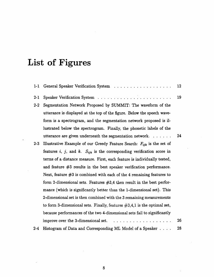
List of Figures
1-1 General Speaker Verification System . ................. 12
2-1 Speaker Verification System ....................... 19
2-2 Segmentation Network Proposed by SUMMIT: The waveform of the
utterance is displayed at the top of the figure. Below the speech wave-
form is a spectrogram, and the segmentation network proposed is il-
lustrated below the spectrogram. Finally, the phonetic labels of the
utterance are given underneath the segmentation network. ...... . 24
2-3 Illustrative Example of our Greedy Feature Search: Fijk is the set of
features i, j, and k. Sijk is the corresponding verification score in
terms of a distance measure. First, each feature is individually tested,
and feature #3 results in the best speaker verification performance.
Next, feature #3 is combined with each of the 4 remaining features to
form 2-dimensional sets. Features #3,4 then result in the best perfor-
mance (which is significantly better than the 1-dimensional set). This
2-dimensional set is then combined with the 3 remaining measurements
to form 3-dimensional sets. Finally, features #3,4,1 is the optimal set,
because performances of the two 4-dimensional sets fail to significantly
improve over the 3-dimensional set. . .................. 26
2-4 Histogram of Data and Corresponding ML Model of a Speaker . . .. 28
2-5 Speaker FO Models and Cohorts: '-' models represent the true female
speaker and '-.' models are 5 of her cohorts. The '.' models represent
a female outlier and the '+' models represent a male outlier of the true
speaker's cohort set.............................
2-6 Speaker Verification Testing Procedure . ................
3-1 ROC Curve for Energy and Corresponding Performance Distance
3-2 Distances for 1-Dimensional Feature Sets
3-3
3-4
3-5
3-6
3-7
3-8
3-9
3-10
3-11
Duration models of 4 Speakers . . . . . . . . . . . . . ...
Energy models of 4 Speakers . . . . . . . . . . . ......
Distances for 2-Dimensional Feature Sets . . . . . . . . . .
Distances for 3-Dimensional Feature Sets . . . . . . . . . .
Distances for 6-Dimensional Feature Sets . . . . . . . . . .
Distances for 7-Dimensional Feature Sets . . . . . . . . . .
Distances for Best Feature Sets of Each Search Stage . .
Distances for the First Stage of Search using New Data . .
Distances for the Second Stage of Search using New Data .
3-12 ROC Curves Using 168 Speakers and Normalizing Results Using 14
Cohorts ..................................
4-1 ROC curves for Optimal Feature Set: Models are trained on TIMIT
data and tested on either TIMIT or NTIMIT . .............
4-2 ROC curves for the Optimal Feature Set Before and After Adaptation
A-i MFSC Filter Banks ............................
A-2 Block Diagram for Computing MFCCs . ................
B-I Production of Speech Signals . ......................
B-2 The Autocorrelation Function of the Error Residual for a Short Time
Interval .................................
. . . . . . . 38
. . . . . . 39
. . . . . . 40
. . . . . . 41
. . . . . . 42
. . . . . . 43
. . . . . . 45
. . . . . . 46
. . . . . . 49
. . . . . . 51
List of Tables
2-1 Phone Distributions of Broad Manner Classes . . . . . . . . . . . . .
3-1 One Dimensional Feature Set Results . . . . . . . . . . . . . . . . . .
3-2 Average Mahalanobis Distances for 4 Speakers' Duration and Energy
M odels . . . . . . . . . . . . . . . . . . . . . . . . . . . . . . . . . . .
3-3 One Dimensional Feature Set Results . . . . . . . . . . . . . . . . . .
3-4 Two Dimensional Feature Set Results . . . . . . . . . . . . . . . . . .
3-5 Comparing SUMMIT to an HMM and Neural Network System . . .
3-6 Number of Training Parameters .....................
C-1
C-2
C-3
C-4
C-5
C-6
Two Dimensional Feature Set Results .
Three Dimensional Feature Set Results
Four-Dimensional Feature Set Results.
Five-Dimensional Feature Set Results
Six Dimensional Feature Set Results
Seven Dimensional Feature Set Results
. . . . . . . . . . . . 72
.. . . . . . . . . . . 73
. . . . . . . . . . . . 73
. . . . . . . . . . . . 73
. . . . . . . . . . . . 74
. . . . . . . . . . . . 74

Chapter 1
Speaker Verification
1.1 Introduction
Speaker verification involves the task of automatically verifying a person's identity by
his/her speech through the use of a computer. The outcome of speaker verification is
a binary decision as to whether or not the incoming voice belongs to the purported
speaker. Speaker verification has been pursued actively by researchers, because it is
presently a palpable task with many uses that involve security access authorizations.
In the past, applications for speaker verification systems mainly involved physical
access control, automatic telephone transaction control (e.g., bank-by-phone), and
computer data access control. However, due to the revolution in telecommunications,
uses for speaker verification systems also include Internet access control, and cellular
telephone authorizations.
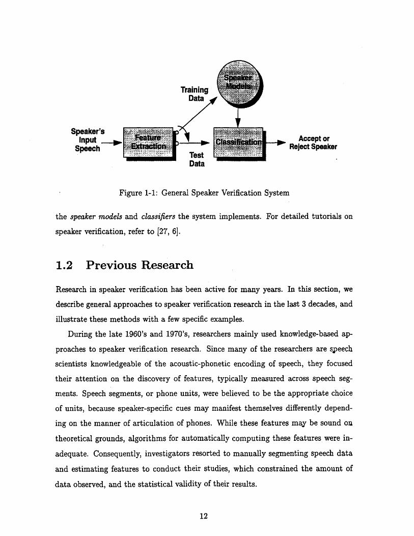
Figure 1-1 illustrates the basic components of a speaker verification system. The
feature extraction component attempts to capture acoustic measurements from the
user's speech signal that are relevant to inter-speaker differences. During training,
the acoustic features are used to build speaker-specific models. During testing, mea-
surements extracted from the test data are scored against the stored speaker models
to see how well the test data match the reference models. The speaker is accepted or
rejected based on this score. Of.course, many details are left out of the block diagram,
such as the type of text the system prompts, the features the system extracts, and
TrainingData
Speaker',Input
SpeechAccept or
Reject Speaker
Figure 1-1: General Speaker Verification System
the speaker models and classifiers the system implements. For detailed tutorials on
speaker verification, refer to [27, 6].
1.2 Previous Research
Research in speaker verification has been active for many years. In this section, we
describe general approaches to speaker verification research in the last 3 decades, and
illustrate these methods with a few specific examples.
During the late 1960's and 1970's, researchers mainly used knowledge-based ap-
proaches to speaker verification research. Since many of the researchers are speech
scientists knowledgeable of the acoustic-phonetic encoding of speech, they focused
their attention on the discovery of features, typically measured across speech seg-
ments. Speech segments, or phone units, were believed to be the appropriate choice
of units, because speaker-specific cues may manifest themselves differently depend-
ing on the manner of articulation of phones. While these features may be sound on
theoretical grounds, algorithms for automatically computing these features were in-
adequate. Consequently, investigators resorted to manually segmenting speech data
and estimating features to conduct their studies, which constrained the amount of
data observed, and the statistical validity of their results.
One example of research done in this era is the doctoral thesis of Wolf [40]. Wolf
found specific segmental measurements that discriminated well among speakers. He
investigated 17 different features such as, fundamental frequency (FO), glottal source
spectral slopes, duration, and features characterizing vowel and nasal spectra. During
training, 21 male speakers repeated 6 short sentences 10 times. Nine of the repetitions
of each utterance were used to develop speaker templates consisting of means and
variances of the features. The remaining sentences were used to test the speakers.
During testing, Euclidean distances between test data and speaker templates were
used to classify speakers. Wolf used the F-ratio analysis of variance to evaluate the
speaker-discriminating abilities of the measurements. The F-ratio is a weighted ratio
of the variance of speaker means to the average of speaker variances. Wolf found that
features with high F-ratios resulted in 100% speaker classification accuracy.
Wolf's study showed that segment-based features discriminate well among speak-
ers. Using phonetic units is also advantageous, because the verification can be inde-
pendent of the particular words the users says. However, Wolf extracted the features
from manually segmented speech data. Consequently, he could not build an auto-
mated speaker verification system that derived the benefits of his knowledge-based
approach. Other studies that also used knowledge-based approaches to speaker veri-
fication are described in [37, 14].
In the 1980s, researchers abandoned the notion of using segment-based measure-
ments for speaker verification, because algorithms to automatically segment speech
remained inadequate. Instead, investigators began using measurements that are easily
computed automatically, such as features extracted from speech frames. Frame-based
features may not necessarily distinguish speakers well. However, these measurements
allowed researchers to build automated systems. These systems typically modeled
speakers with word templates. The templates represented speech frames of words
with feature centroids. Just as before, speakers were classified with distances com-
puted between test feature vectors and centroids.
One of the earliest automated speaker verification systems was implemented in the
early 1980's at Texas Instruments (TI) corporate headquarters in Dallas, Texas [6].
The system automatically computed features from 6 frames for each word, regardless
of the word's duration. Specifically, each frame used the output of a 14 channel filter
bank, uniformly spaced between 300 and 3000Hz, as a 14x1 spectral amplitude feature
vector. During training, templates for 16 words were constructed for each speaker.
During testing, the system prompted 4-word utterances constructed randomly from
the 16 word bank. A Euclidean distance between measurements of test frames and
reference frames was then computed, and used to make a verification decision. At the
time, the system achieved 99.1% acceptance rate of valid users, and 0.7% acceptance
rate of impostors. Similar speaker verification systems that use template matching
classification techniques are described in [15, 9].
As mentioned above, these pioneering systems typically modeled words with tem-
plates for each speaker. Templates do not capture variations in the acoustic feature
space, because each frame is represented by a fixed acoustic centroid. Consequently,
the templates are not robust models of speech. In addition, the system is dependent
on the words the users says during verification.
In the early 1990s, statistical models of speech became popular for speech recog-
nition, because the models represent the acoustic feature space with a distribution,
rather than a fixed centroid. As a result, researchers began applying the technology to
speaker verification. Specifically, speaker verification research focused on investigat-
ing hidden Markov models (HMMs), because HMMs were becoming very successful in
speech recognition [32]. Many investigators simply modified existing speech recogni-
tion systems for speaker verification, in hopes of achieving high performance. HMMs
are developed from frame-based features; therefore, investigators neglected to further
explore segment-based features. In fact, most of the studies use frame-based cepstral
measurements, and compare different HMM speaker models to each other.
An HMM models speech production as a process that is only capable of being in
a finite number of different states, and each state generates either a finite number of
outputs or a continuum of outputs. The system transitions from one state to another
at discrete intervals of time, and each state produces a probabilistic output [27]. In a
speaker verification system, each speaker is typically represented by an HMM, which
may capture statistics of any component of speech such as a sub-phone, phone, sub-
word, word etc. To verify the speaker, the test sentence is scored by the HMM. The
score represents the probability of an observation sequence, given a test sequence and
a speaker HMM.
Furui and Matsui investigated various HMM systems for speaker verification. In
one study [25], they built a word-independent speaker verification system and com-
pared discrete HMM to continuous HMM speaker models. The speaker verification
system computed frame-based cepstral features, and the corpus consisted of 23 male
and 13 female speakers, recorded during three sessions over a period of 6 months. Ten
sentences were used to train both continuous and discrete HMMs for each speaker, and
5 sentences were used to test the speakers. During testing, the purported speaker's
cumulative likelihood score was used to make a verification decision. Furui and Mat-
sui reached a performance of 98.1% speaker verification rate, using continuous HMMs.
Other studies that are based on HMMs include [24, 35, 34].
Recently, investigators have applied other statistical methods, such as neural net-
works, to speaker verification. Neural networks have also been successful in other
tasks, such as speech and handwriting recognition. They are statistical pattern
classifiers that utilize a dense interconnection of simple computational elements, or
nodes [20]. The layers of nodes operate in parallel, with the set of node outputs in
a given layer providing the inputs to each of the nodes in a subsequent layer. In a
speaker verification system, each speaker is typically represented by a unique neural
network. When a test utterance is applied, a verification decision is based on the
score for the speaker's models. Some examples of systems that use neural networks
to represent and classify speakers are [41, 3, 18, 28, 36].
1.3 Discussion
Thirty years ago, researchers manually computed segment-based acoustic features,
and modeled the speech signal with templates consisting of acoustic centroids. Presently,
systems automatically compute frame-based acoustic features, and use statistical
models to represent the speech signals, such as HMMs and neural networks. As Matsui
and Furui showed in one of their studies [25], most statistical methods give improved
performance over template methods. In addition, frame-based measurements are easy
to compute and are successful in speaker verification. However, segment-based fea-
tures have been proven to carry speaker-specific cues, and may result in equivalent
performance with less dimensionality.
1.4 Thesis Objective and Outline
The ultimate goal of speaker verification research is to develop user-friendly, high per-
formance systems, that are computationally efficient and robust in all environments.
In this study, we strive to develop a competitive segment-based speaker verification
system that requires minimal computation. We automatically compute segment-
based measurements, and use statistical models of speech to represent speakers. Es-
sentially, we combine two successful approaches to speaker verification, knowledge-
based and statistical. As a result, we hope to achieve competitive speaker verification
performance with minimal computation. We do not investigate robustness issues
specifically. However, we explore acoustic features that have been proven to be ro-
bust in the past, such as fundamental frequency and energy [41, 17].
To achieve our goal, we modified SUMMIT, a state-of-the-art speech recognition
system developed at MIT [43], for speaker verification. We chose SUMMIT for the
following reasons. First, SUMMIT treats the speech signal as a concatenation of
segments, which allows us to capitalize on the speaker-discriminating abilities of such
units. Second, SUMMIT allows us to model the features statistically; therefore we
can also capture feature-varying attributes in the speech signal. Finally, SUMMIT
employs search algorithms, which allows us to modify the algorithms to conduct a
search for an optimal feature set. We search for an optimal feature set from an initial
pool of measurements, which include cepstral and prosodic measurements.
Details of our speaker verification system and its design are given in chapter 2.
The system description is followed by a presentation of our experimental results and
analysis in chapter 3. Finally, chapter 4 summarizes conclusions of our system results,
and proposes future work in speaker verification.
Chapter 2
System Description
2.1 Introduction
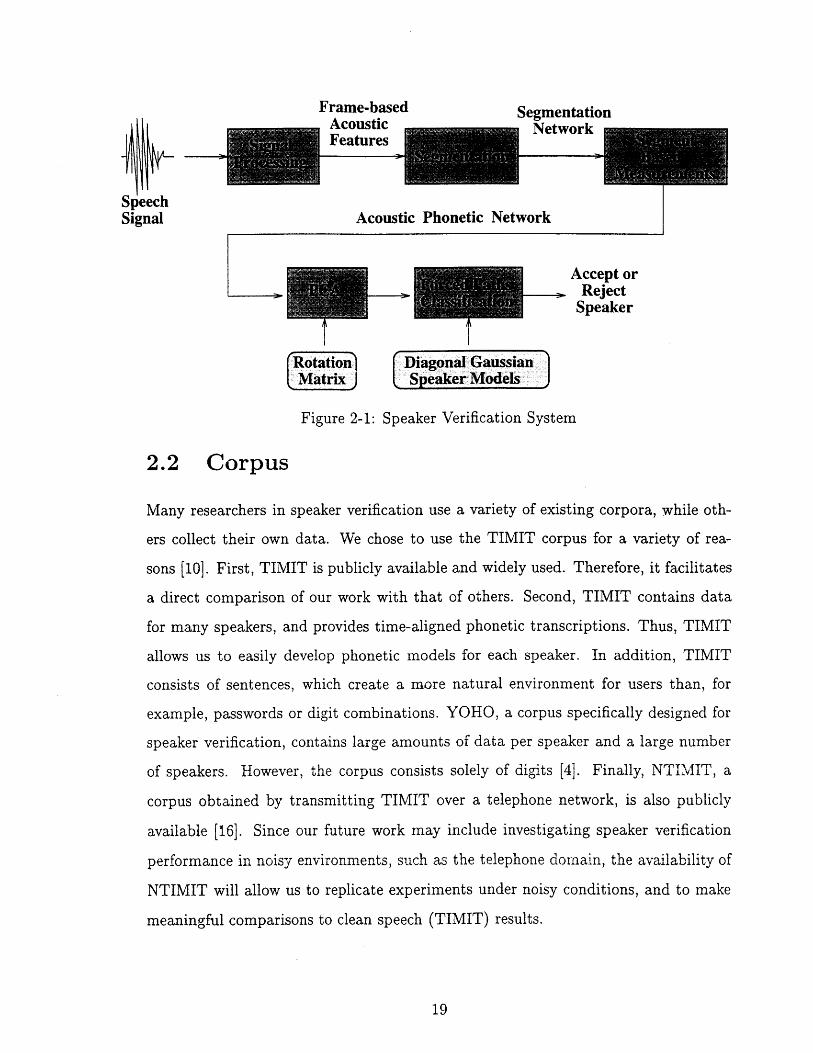
In this chapter, we describe the components of our speaker verification system. Fig-
ure 2-1 summarizes our system with a block diagram, whose building blocks are
components of SUMMIT, modified to suit our needs. Initially, signal processing trans-
forms the speech samples to frame-based acoustic features. These features are then
used to propose a segmentation network for the utterance. Next, the acoustic mea-
surements are averaged across segments, and rotated into a space that de-correlates
them, via principal components analysis (PCA) (section 2.6). During training, di-
agonal Gaussian speaker models are developed. During testing, the speaker models
are used to compute forced alignment scores (section 2.7.3) for test utterances. Fi-
nally, the scores (section 2.7.3) are used to classify speakers, and make a verification
decision.
This chapter begins with a description of the corpus used to train and evaluate
our system. Next, the acoustic features selected to represent the speech signal are
discussed. Thereafter, the algorithm used to create a segmentation network from
the frame-based features is described, and followed by a discussion of a search for an
optimal set of segment-based measurements. Finally, details are given on how speaker
models were developed, and how speakers were classified.
Frame-based Se m
-~/~fr-SpeechSignal
TIrRotation ( Diagonal Gaussian
Matrix peakerModels
Figure 2-1: Speaker Verification System
2.2 Corpus
Many researchers in speaker verification use a variety of existing corpora, while oth-
ers collect their own data. We chose to use the TIMIT corpus for a variety of rea-
sons [10]. First, TIMIT is publicly available and widely used. Therefore, it facilitates
a direct comparison of our work with that of others. Second, TIMIT contains data
for many speakers, and provides time-aligned phonetic transcriptions. Thus, TIMIT
allows us to easily develop phonetic models for each speaker. In addition, TIMIT
consists of sentences, which create a more natural environment for users than, for
example, passwords or digit combinations. YOHO, a corpus specifically designed for
speaker verification, contains large amounts of data per speaker and a large number
of speakers. However, the corpus consists solely of digits [4]. Finally, NTIMIT, a
corpus obtained by transmitting TIMIT over a telephone network, is also publicly
available [16]. Since our future work may include investigating speaker verification
performance in noisy environments, such as the telephone domain, the availability of
NTIMIT will allow us to replicate experiments under noisy conditions, and to make
meaningful comparisons to clean speech (TIMIT) results.
'' -- -b--entati n~A ^,%mvý+vrnentation
2.2.1 TIMIT
TIMIT consists of 630 speakers, 70% male and 30% female, who represent 8 major
dialect regions of the United States. We selected a subset of 168 speakers (TIMIT's
standard NIST-test and NIST-dev sets) for evaluation. Each speaker read a total of
10 sentences, 2 dialect (SA), 5 phonemically rich (SX), and 3 other (SI) sentences.
The 2 SA utterances are the same across all speakers, while the 3 SI sentences are
unique to each speaker. A collection of 450 SX sentences in TIMIT are each read
by 7 speakers, whereas 1890 sentences from the Brown corpus were each read by
one speaker. We used 8 sentences (SX,SI) to develop each speaker model, and the
remaining 2 SA sentences to test each speaker. Since 8 utterances may not adequately
model a speaker's sound patterns, it is necessary to compensate for the lack of training
data. In this study, the complexity of the speaker models is reduced by forming broad
phonetic classes.
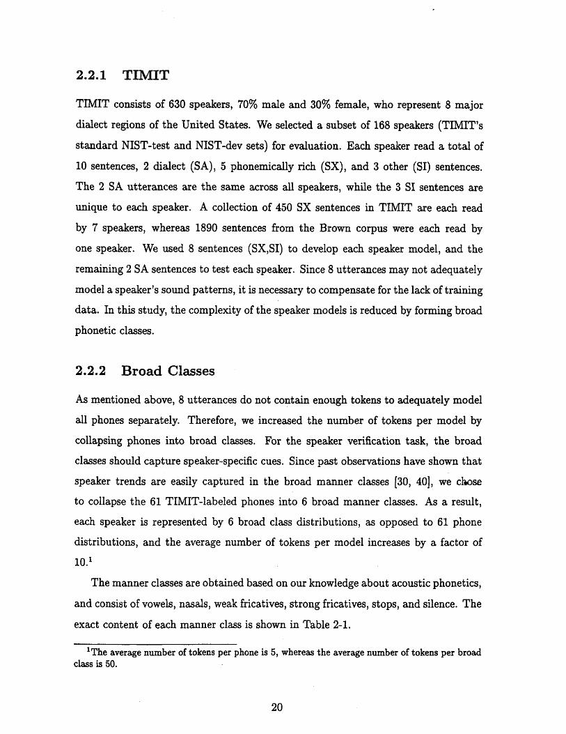
2.2.2 Broad Classes
As mentioned above, 8 utterances do not contain enough tokens to adequately model
all phones separately. Therefore, we increased the number of tokens per model by
collapsing phones into broad classes. For the speaker verification task, the broad
classes should capture speaker-specific cues. Since past observations have shown that
speaker trends are easily captured in the broad manner classes [30, 40], we chose
to collapse the 61 TIMIT-labeled phones into 6 broad manner classes. As a result,
each speaker is represented by 6 broad class distributions, as opposed to 61 phone
distributions, and the average number of tokens per model increases by a factor of
10.1
The manner classes are obtained based on our knowledge about acoustic phonetics,
and consist of vowels, nasals, weak fricatives, strong fricatives, stops, and silence. The
exact content of each manner class is shown in Table 2-1.
1The average number of tokens per phone is 5, whereas the average number of tokens per broadclass is 50.
CLASS PHONESVowels iy,ih,eh,aa,ay,ix,ey,oy,aw,w,r,1,el,er,ah,ax,ao,ow,uh,axr,ax-
h,ux,ae
Stops b,d,g,p,t,k
Nasals m,em,n,en,nx,ng,eng,dx,q
Strong Frics s,sh,z,zh,ch,jh
Weak Frics f,th,dh,v,hh,hv
Silence pcl,tcl,kcl,bcl,dcl,gcl,pau,epi,h#
Table 2-1: Phone Distributions of Broad Manner Classes
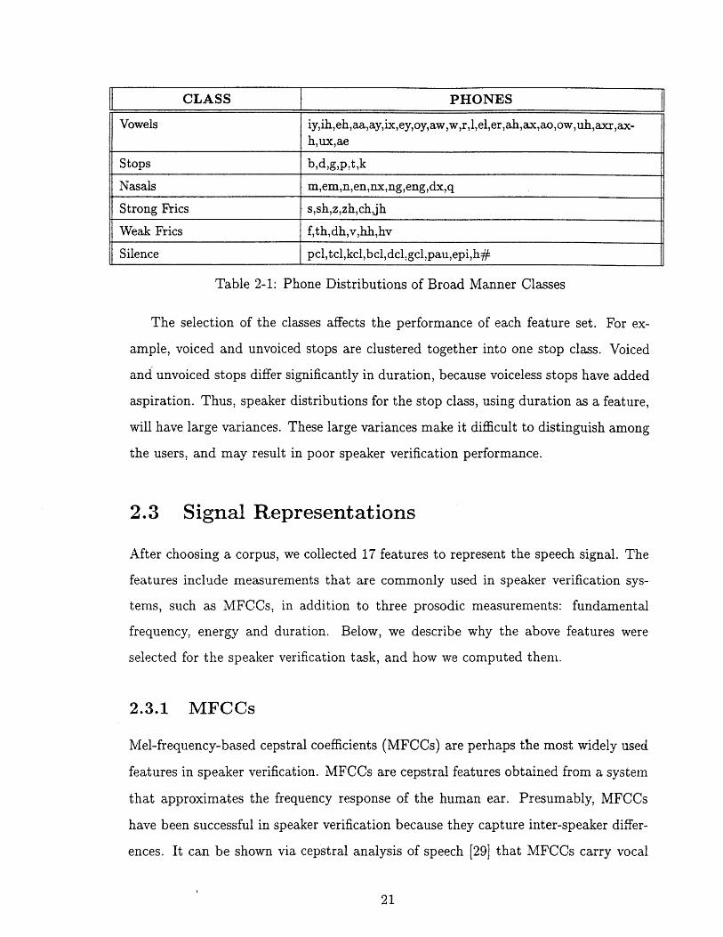
The selection of the classes affects the performance of each feature set. For ex-
ample, voiced and unvoiced stops are clustered together into one stop class. Voiced
and unvoiced stops differ significantly in duration, because voiceless stops have added
aspiration. Thus, speaker distributions for the stop class, using duration as a feature,
will have large variances. These large variances make it difficult to distinguish among
the users, and may result in poor speaker verification performance.
2.3 Signal Representations
After choosing a corpus, we collected 17 features to represent the speech signal. The
features include measurements that are commonly used in speaker verification sys-
tems, such as MFCCs, in addition to three prosodic measurements: fundamental
frequency, energy and duration. Below, we describe why the above features were
selected for the speaker verification task, and how we computed them.
2.3.1 MFCCs
Mel-frequency-based cepstral coefficients (MFCCs) are perhaps the most widely used
features in speaker verification. MFCCs are cepstral features obtained from a system
that approximates the frequency response of the human ear. Presumably, MFCCs
have been successful in speaker verification because they capture inter-speaker differ-
ences. It can be shown via cepstral analysis of speech [29] that MFCCs carry vocal

tract information (i.e., formant frequency locations), as well as fundamental frequency
information. The vocal tract system function is dependent on the shape and size of
the vocal tract, which is unique to a speaker and the sound that is being produced.
Fundamental frequency (FO) also carries speaker-specific information, because FO is
dependent on accents, different phonological forms, behavior and other individualistic
.factors [41, 1].
To compute MFCCs, the speech signal was processed through a number of steps.
First, the digitized utterances were initially passed through a pre-emphasis filter,
which enhances higher frequency components of the speech samples, and attenuates
lower frequency components. Next, a short time Fourier transform (STFT) of the
samples was computed at an analysis rate of 200 Hz, using a 20.5 ms Hamming
window. The STFT thus produced one frame of spectral coefficients every 5 seconds.
Then, each of the coefficients was squared component-wise to produce the power
spectral density (PSD) for each frame. Thereafter, the logarithm of the PSD was
computed and the resulting coefficients were processed by an auditory filter bank,
which produced mel-frequency spectral coefficients (MFSCs). Finally, the MFSCs
were rotated by the discrete cosine transform (DCT) matrix. The matrix transformed
the mel-frequency spectral coefficients (MFSCs) to 14 less correlated MFCCs. More
details are given in Appendix A.
2.3.2 Prosodic Features
In addition to MFCCs, we decided to explore three prosodic features: fundamental fre-
quency (FO), energy and duration. These features attempt to measure psychophysical
perceptions of intonation, stress, and rhythm, which are presumably characteristics
humans use to differentiate between speakers [6]. Prosodic features have also proven
to be robust in noisy environments [41, 17, 1]. Therefore, these features show great
potential for the speaker verification task.
To estimate FO, we used the ESPS tracker, in particular the FORMANT func-
tion [7]. For each frame of sampled data, FORMANT estimates speech formant tra-
jectories, fundamental frequency, and other related information. The ESPS formant
tracker implements the linear prediction analysis method, described in Appendix B, to
estimate FO. FORMANT also uses dynamic programming and continuity constraints
to optimize the estimates of FO over frames. Although the tracker also estimates
probabilities of voicing for each frame, we retained FO information for every frame,
regardless of whether the underlying sounds were voiced or unvoiced.
To compute energy, the power spectral density coefficients for each frame, obtained
in the same manner as described in section 2.3.1, were summed. We computed the
logarithm of this sum to convert energy to the decibel (dB) scale. The logarithm of
duration was also computed in our experiments.
2.4 Segmentation
Once frame-based acoustic features are computed, the system proposes possible seg-
mentations for the utterance. The goal of the segmenter is to prune the segment
search space using inexpensive methods, without deleting valid segments. During
segmentation, frame-based MFCCs are used to first establish acoustic landmarks in
the utterance. Then, a network of possible acoustic-phonetic segments are created
from the landmarks.
Acoustic landmarks are established in two steps. First, the algorithm identifies
regions of abrupt spectral changes, and places primary landmarks at these locations.
Next, secondary landmarks are added to ensure that a specified number of boundaries
are marked within a given duration. To create the network of possible acoustic-
phonetic segments, the procedure then fully connects all possible primary landmarks
for every deleted secondary landmark.
An analysis of the networks proposed using this algorithm shows that on a devel-
opment set, there are an average of 2.4 landmarks proposed for every transcription
landmark, and 7 segments hypothesized for every transcription segment [12]. The
multi-level description of the segmentation is illustrated in Figure 2-2 for the utter-
ance "Delta three fifteen". The segmentation algorithm is described in more detail
in [11].
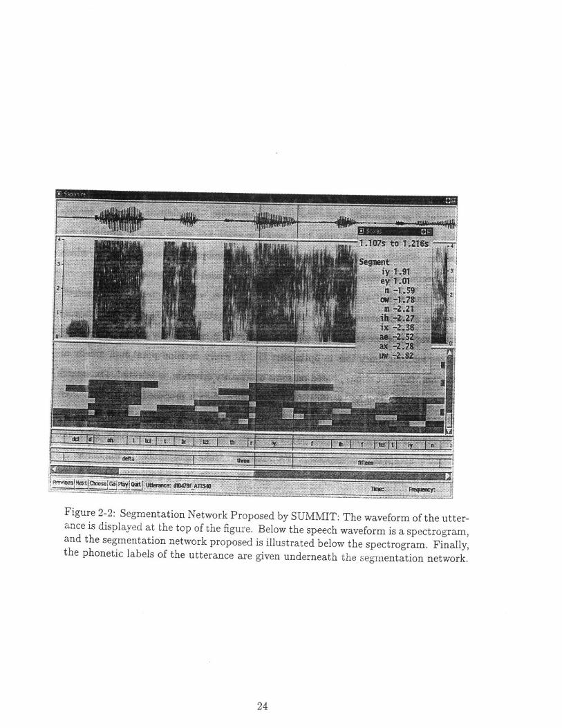
Figure 2-2: Segmentation Network Proposed by SUMMIT: The waveform of the utter-ance is displayed at the top of the figure. Below the speech waveform is a spectrogram,and the segmentation network proposed is illustrated below the spectrogram. Finally,the phonetic labels of the utterance are given underneath the segmentation network.
24
2.5 Measurement Search
Each of the segments proposed by the segmentation algorithm is described by a set
of acoustic features. The set of 17 measurements discussed above represents a pool of
possible features to characterize segments. We did not use all 17 measurements in the
system for the following reasons. First, some features may be useful in discriminating
speakers well, while others may not. Second, some of the measurements may be
correlated or essentially carry the same information. In addition, training models
with high dimensionality may be a problem since not much data is available per
speaker. Finally, computation increases as the number of features increases, which
may become expensive if all 17 measurements are used in the system.
To find a (sub)-optimal subset of the 17 features, we conducted a greedy search,
because an exhaustive search is computationally prohibitive. A greedy search may
not always produce an optimal solution. However, it significantly prunes large search
spaces without much loss in optimality [5]. At every decision point in a greedy al-
gorithm, the best choice, based on some optimality criterion, is selected. Our search
criterion is the speaker verification performance of each proposed feature set. Per-
formance is measured in terms of a distance metric describe in detail in section 3.2.
The measure minimizes the two types of errors, false rejection of true users (FR) and
the false acceptance of impostors (FA). However, false acceptances of impostors are
considered more costly. Below, we describe the greedy feature search, which is also
illustrated in Figure 2-3 for an initial pool of 5 features.
The search algorithm begins by obtaining FR rates and FA rates for the 168 test
speakers, using each of the 17 features. Thus we obtain 17 performance results cor-
responding to each measurement. The feature that results in the smallest distance
measure (best performance) is chosen as the best 1-dimensional measurement. Next,
the best 1-dimensional feature is combined with each of the remaining measurements.
Two-dimensional feature sets are grouped in this fashion, and are each used to test
the 168 speakers. The best 2-dimensional feature vector, in terms of speaker verifica-
tion performance, is then used for the next stage of the search. The search continues
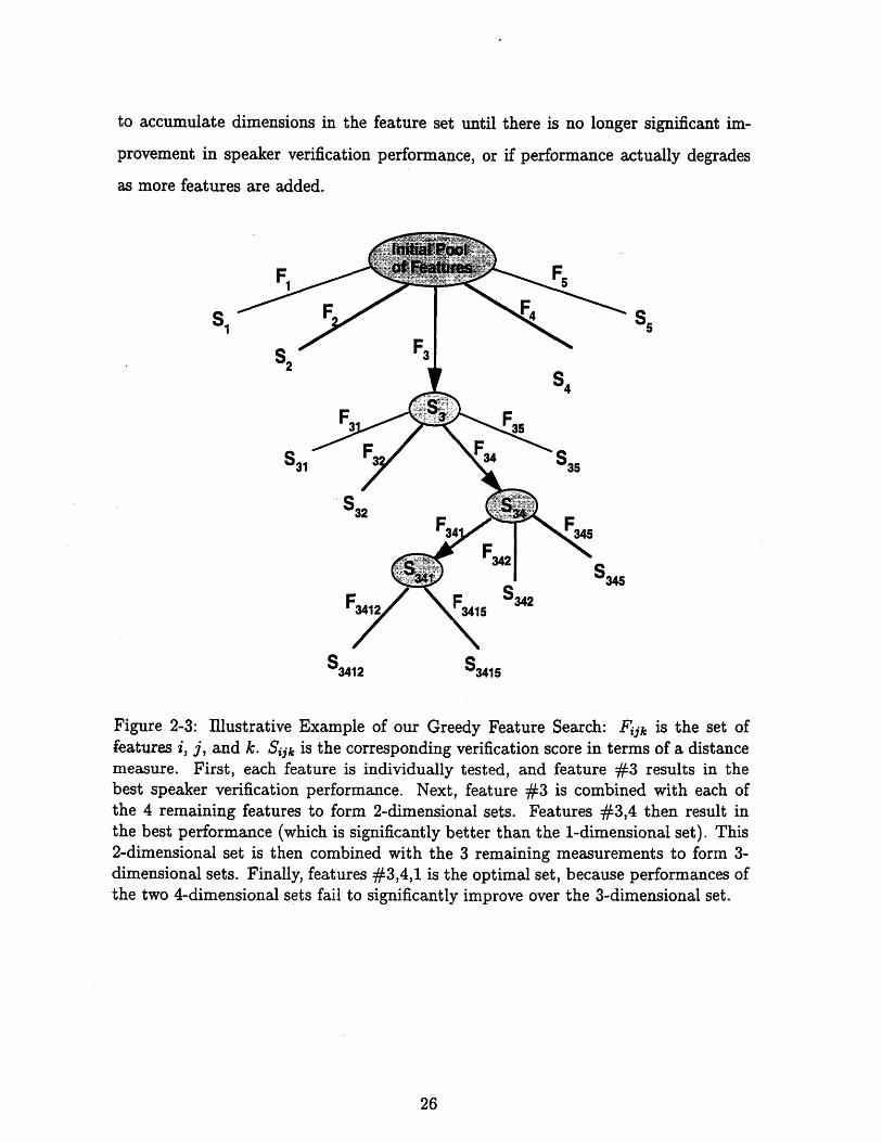
to accumulate dimensions in the feature set until there is no longer significant im-
provement in speaker verification performance, or if performance actually degrades
as more features are added.
S3412 S3415
Figure 2-3: Illustrative Example of our Greedy Feature Search: Fijk is the set offeatures i, j, and k. Sijk is the corresponding verification score in terms of a distancemeasure. First, each feature is individually tested, and feature #3 results in thebest speaker verification performance. Next, feature #3 is combined with each ofthe 4 remaining features to form 2-dimensional sets. Features #3,4 then result inthe best performance (which is significantly better than the 1-dimensional set). This2-dimensional set is then combined with the 3 remaining measurements to form 3-dimensional sets. Finally, features #3,4,1 is the optimal set, because performances ofthe two 4-dimensional sets fail to significantly improve over the 3-dimensional set.

2.6 Speaker Models
During training, statistical models of segment-based acoustic features are developed
for each speaker. Specifically, the speaker models consist of diagonal Gaussian proba-
bility density functions (pdfs). We chose to represent the acoustic space with Gaussian
distributions because features of speech data, such as cepstral coefficients, fit these
bell-shaped curves well [381. Diagonal distributions were implemented because they
have few parameters to train (diagonal covariance matrices), and thus do not require
much training data to accurately estimate the parameters. However, features that
are correlated are not modeled well with diagonal covariance matrices.
To ensure that the features fit the diagonal models better, principal components
analysis (PCA) was performed on the acoustic features before developing the models.
PCA rotates a d-dimensional space to a set of orthogonal dimensions (less than or
equal to the dimension d). As a result, the full covariance matrix of the original space
is transformed to a diagonal matrix in the new space. In principle, PCA also allows
us to reduce the dimensionality of the feature vectors. However, in our experiments,
we did not reduce dimensionality with PCA since the feature search already prunes
the number of features used in the system.
The Gaussian distributions that model the acoustic features for each speaker are
developed using the maximum likelihood (ML) estimation procedure. The mathe-
matical expressions for the ML estimates for the means, variances and the a priori
class probability estimates for a particular speaker model are shown below. An ex-
ample of a speaker model developed using the ML procedure is shown in Figure 2-4.
Figure 2-4 illustrates a histogram of a speaker's training data and the corresponding
model developed. It is apparent that a single diagonal Gaussian cannot completely
model the data for each class. Mixtures of diagonal Gaussians may fit the data better.
However, there are more parameters to train mixtures of Gaussians, which require
more data than are available.
j = the jth broad class
nj = the number of tokens for class j

n = the total number of tokens for all classes
Xj,k = the kth data token for class j
Pj = the ML estimate of the mean for class j
-6F = the ML estimate of the variance for class j
P(j) = a priori probability for class j
k=11 n"173= (Xij,k
P(j) = njn
stops
40 50 60 70 80 90 100
40 50 60 70 80 90 100
1 - 1
40 50 60 70 80 90 100energy
10 -
30 40 50 60 70 80 90 100
,20Wieri
10 "
30 40 50 60 70 80 90 100
10
s-irncs
30 40 50 60 70 80 90 100energy
Figure 2-4: Histogram of Data and Corresponding ML Model of a Speaker
2.7 Speaker Classification
Once speaker models are developed, test utterances are scored against these models
to classify speakers and make verification decisions. Below we describe our testing
conditions, which use the concept of cohort normalization. Next, we describe the
verification process and conclude with a description of how scores are computed.
0 15-0 I
0'30
60
20
30
AAIII.
i
2.7.1 Cohort Sets
During testing, it is ideal to compare the utterances to all speaker models in the
system, and accept the purported speaker if his/her model scores best against the
test data. However, computation becomes more expensive as speakers are added to
the system. Since speaker verification is simply a binary decision of accepting or
rejecting a purported speaker, the task should be independent of the user population
size.
To keep our system independent of the number of users and computationally
efficient, we implemented a technique called cohort normalization. For each speaker,
we pre-detected a small set of speakers, called a cohort set, who are acoustically
similar to the purported speaker.2 During testing, we only test the speakers in the
cohort set for the purported speaker. Speakers outside the cohort set are considered
outliers that have low probabilities of scoring well against the purported speaker's
test data. Therefore, results using just cohorts during testing may minimally affect
speaker verification performance, and can be normalized to emulate results using all
speakers during testing. Detailed results of the normalization are given in section 3.4.
For each feature set, we found S nearest neighbors (cohorts) for each speaker
using the Mahalanobis distance metric [39]. Specifically, pi and P2, o~ and a , are
d-dimensional mean vectors and dxd-dimensional covariance matrices for two speaker
models, respectively. The Mahalanobis distance squared, D2, between the two speak-
ers is then
D2(1, 2) = (Ai -P2i)2i=1
where
2 22= +lai 2a2i
nl + n 2 nl + n2
2The size of each cohort set is a parameter we varied in our experiments.
and nl and n2 are the number of data vectors for speaker one and speaker two,
respectively.
Once the speaker models were developed, this metric was applied to every possible
pair of speakers. The distances were then sorted for each speaker, and the cohorts
were chosen to be the S closest neighbors to each speaker.
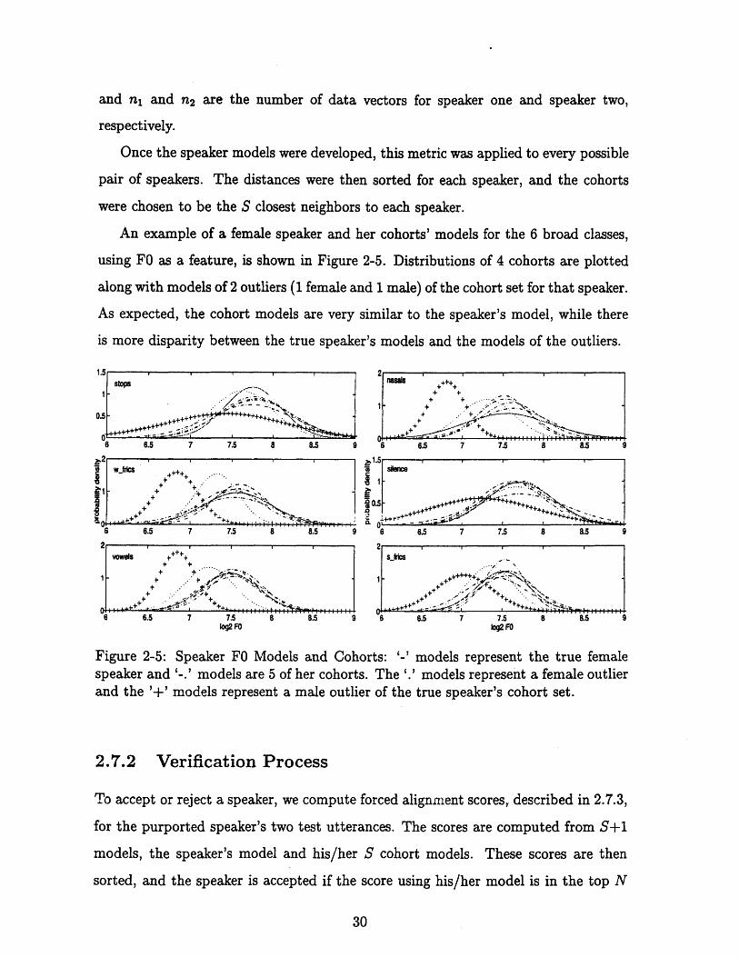
An example of a female speaker and her cohorts' models for the 6 broad classes,
using FO as a feature, is shown in Figure 2-5. Distributions of 4 cohorts are plotted
along with models of 2 outliers (1 female and 1 male) of the cohort set for that speaker.
As expected, the cohort models are very similar to the speaker's model, while there
is more disparity between the true speaker's models and the models of the outliers.
++ 4. - ,
S +
6.5 7 7.5 8 8.5
wels +++++ +
+ + ' .. ,
4. -:,- ' ". ,
6.5 7 7.5 8 8.51og2 FO
2 nsal ++++i+ +
+ +
+ 4, + -. ....• '.• -· .P ./ .• _. ,.,. ,4.4. .. ,. • - •s.".•.6 6.5 7 7.5 8 8.5 9
I. silence
OI .. ..,. ": ....•iI '••• •0.5 6. +7.++ ++++ +++i+++++++ ~ ++~~ii-~
6 6.5 7 7.5 8 8.5 9
1og2 FO
Figure 2-5: Speaker FO Models and Cohorts: '-' models represent the true femalespeaker and '-.' models are 5 of her cohorts. The '.' models represent a female outlierand the '+' models represent a male outlier of the true speaker's cohort set.
2.7.2 Verification Process
To accept or reject a speaker, we compute forced alignment scores, described in 2.7.3,
for the purported speaker's two test utterances. The scores are computed from S+1
models, the speaker's model and his/her S cohort models. These scores are then
sorted, and the speaker is accepted if the score using his/her model is in the top N
•iw
6SI
6
· · · · ·
PTut·k~-
"'''''
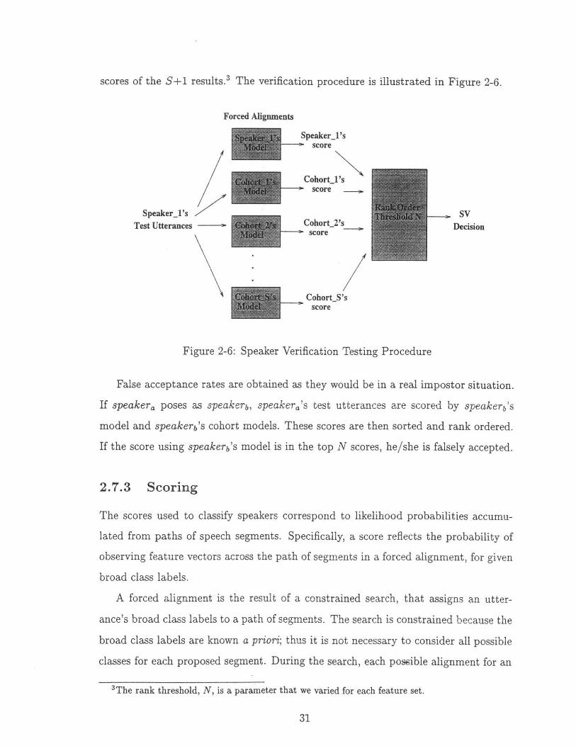
scores of the S+1 results.3 The verification procedure is illustrated in Figure 2-6.
Forced Alignments
/Speaker_l's
- score
I N.
7Z,SpeaKer_'s /s
Test Utterances -
Cohort_l's- score
Cohort_2's- score
SV
Decision
/"
CohortS'sscore
Figure 2-6: Speaker Verification Testing Procedure
False acceptance rates are obtained as they would be in a real impostor situation.
If speakera poses as speakerb, speakera's test utterances are scored by speakerb's
model and speakerb's cohort models. These scores are then sorted and rank ordered.
If the score using speakerb's model is in the top N scores, he/she is falsely accepted.
2.7.3 Scoring
The scores used to classify speakers correspond to likelihood probabilities accumu-
lated from paths of speech segments. Specifically, a score reflects the probability of
observing feature vectors across the path of segments in a forced alignment, for given
broad class labels.
A forced alignment is the result of a constrained search, that assigns an utter-
ance's broad class labels to a path of segments. The search is constrained because the
broad class labels are known a priori; thus it is not necessary to consider all possible
classes for each proposed segment. During the search, each possible alignment for an
3The rank threshold, N, is a parameter that we varied for each feature set.
I \
utterance accumulates likelihood scores. These likelihood scores reflect the probabil-
ities of observing feature vectors across the segments in the alignment, for the given
labels. The path of segments that corresponds to the highest likelihood score, which
is used to classify speakers, is chosen as the forced alignment for the test utterance.
Normally, likelihood scores are accumulated along all possible paths. However,
the system implements the Viterbi algorithm to find the forced alignment without
scoring all possible segmentation paths. The Viterbi algorithm is based on dynamic
programming methods, and prunes the search without any loss in optimality. Details
of the Viterbi algorithm can be found in [33, 5].
Chapter 3 presents the detailed results of our feature search, followed by analysis.
The performance effects of using only cohorts during testing is then illustrated, and
the overall system performance is compared to that of two similar speaker verification
systems.
Chapter 3
Experimental Results & Analysis
3.1 Overview
To evaluate a speaker verification system, it is necessary to observe how performance
is affected as components and test conditions alter. For example, acoustic features,
models and classifiers are system components that affect performance. In our case, we
have limited the scope of our investigation to examining the sensitivity of performance
to acoustic features. We then varied test conditions by observing performances of
features using a different set of speakers.
This chapter first describes performance measures used for speaker verification.
Then, the results of the greedy feature search conducted on the set of 168 test speak-
ers is presented. In addition, we conducted the same experiment using a set of 80
speakers who are not part of the test set to ensure that the feature selection process is
independent of the speakers used. Thereafter, system performance using cohort sets
as well as the performance using the entire test set are reported. Finally, our results
are compared to those of two other systems that are also evaluated on the TIMIT
corpus.

3.2 Performance Measures
The performance of a speaker verification system is typically measured in terms of
two types of errors: false rejections of true users (FR) and false acceptances of im-
postors (FA). Performance is often illustrated with conventional receiver operating
characteristic (ROC) curves, which plot the rates of FR versus the rates of FA for
some varying parameter.
A popular single number measure of performance is the equal error rate (EER),
which is the rate at which the two errors (FR and FA) are equal. EER is thus the
intersection between the ROC curve and the line FR=FA. Many researchers design
speaker verification systems to minimize the EER. However, minimizing this measure
does not allow for different costs to be associated with FA and FR. For high security
applications such as bank-by-phone authorizations, minimizing false acceptances of
impostors is the first priority. Rejecting a true user may annoy the user. However,
accepting an impostor may be costly to the customer.
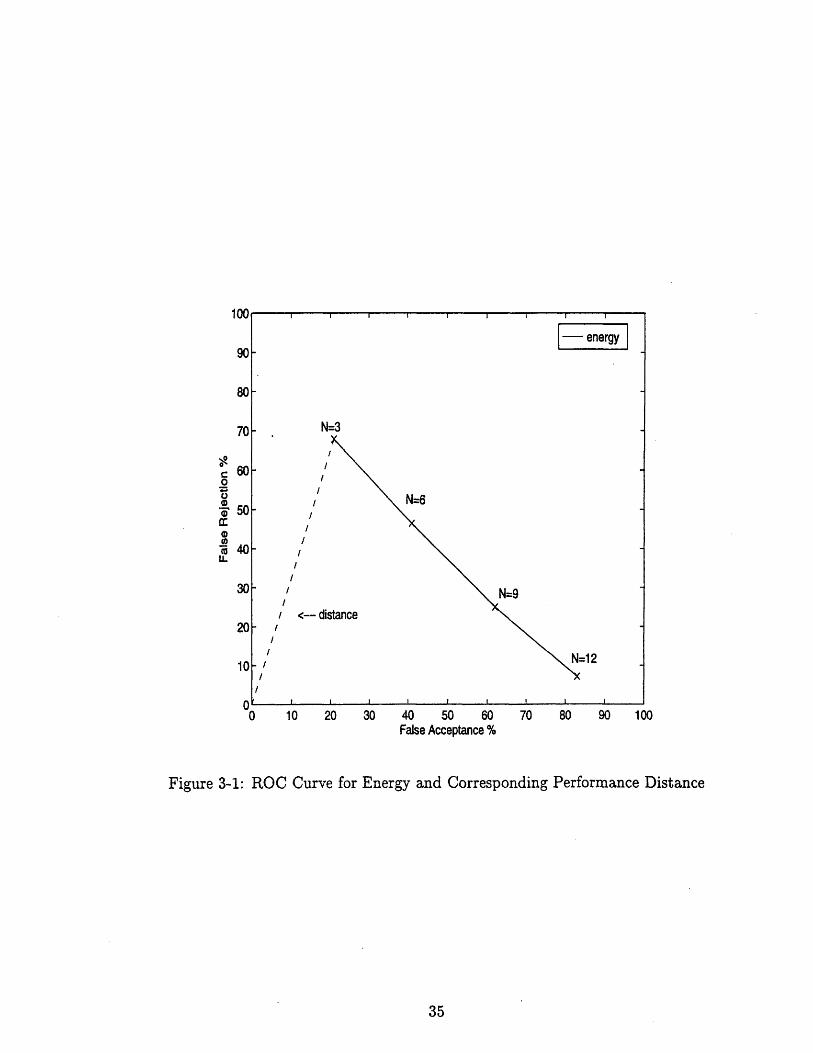
While our goal is to minimize both types of errors, we have chosen to weigh the
cost of false acceptances of impostors more than the cost of false, re-ec=ions of true
users. Specifically, we first obtain the ROC for each feature set by varying the rank
threshold, N (3, 6, 9, 12). The system's performance is then measured in terms of a
distance between the point on the feature's ROC curve that corresponds to the rank
threshold N = 3, to the origin, which corresponds to the ideal performance of 0%
error. Figure 3-1 uses the ROC curve for energy as an example to illustrate how we
computed this distance. The smaller the distance, the more robust the system is to
false acceptances of impostors.
3.3 Feature Search
In this section, we present the results of the greedy feature search using 168 test
speakers, which is followed by a discussion of the seconad p p:tiai serziC c~~dUuctd o n
a different set of 80 speakers. Both searches were conducted using a cohort set size
N3energy
N=3
I
S - i~
'I
0 10 20 30 40 50 60False Acceptance %
70 80 90 100
Figure 3-1: ROC Curve for Energy and Corresponding Performance Distance
I V
90
70
60
50
40
30
20
10 :12
=1II I I | T I I
A ^4%
E
.
-
-
-
-
-
_
of 14, and the results reported are not normalized.'
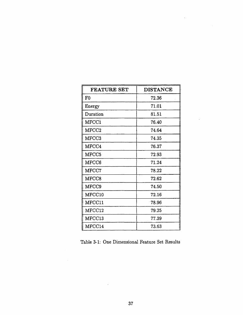
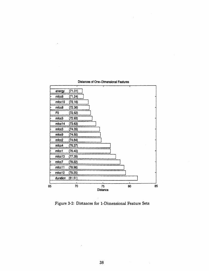
3.3.1 Results Using 168 Speakers
The first stage of the search evaluates the speaker verification performance of in-
dividual features. Performances of the one-dimensional measurements are given in
Table 3-1, and are illustrated in Figure 3-2. Figure 3-2 shows that the top 10 features,
in particular the higher order MFCCs, FO, and energy, result in similar performances.
We disregarded all other features for subsequent search stages, because they resulted
in significantly worse performance than the top 10 features. We realized that such
pruning will result in a search that is not greedy in the strictest sense of the word.
Past observations have shown that MFCCs and prosodic features are useful for
speaker verification [19, 41, 17]. In our search, we found that two of the three prosodic
measurements investigated performed well. Specifically, energy ranked first in the set
of 17 features, and FO ranked fourth. However, duration ranked last in the first stage
of the feature search. Perhaps duration performed poorly because of the way the
broad classes were formed. Many of the 6 manner classes selected, such as stops
and weak fricatives, consist of both voiced and unvoiced phones, which are mainly
distinguished by duration. Consequently, the variances of duration for these classes
are large for all distributions, and the speaker models are often indistinguishable if
the means do not differ by much. As a result, speaker verification performance is
poor.
Figure 3-3 illustrates these large variances (on the order of 10s) of 4 speakers'
duration models of stop consonants and weak fricatives. The 4 speakers are within
a cohort set. Thus, during testing, these speakers are compared to each other and
the remaining members of the cohort set. As shown in Figure 3-3, it is difficult to
reliably distinguish among the 4 distributions. In fact, we computed the average
Mahalanobis distance between the 4 cohort models for the best and worst features,
er::y and duration, respectliey. These distancs azre shown i' Table 3-2, which
1After the search, the normalization is applied to the optimal feature set to obtain the estimatedsystem performance.
FEATURE SET DISTANCE
FO 72.36
Energy 71.01
Duration 81.51
MFCC1 76.40
MFCC2 74.64
MFCC3 74.35
MFCC4 76.37
MFCC5 72.93
MFCC6 71.24
MFCC7 78.22
MFCC8 72.62
MFCC9 74.50
MFCC10 72.16
MFCC11 78.96
MFCC12 79.25
MFCC13 77.39
MFCC14 73.63
Table 3-1: One Dimensional Feature Set Results
Distances of One-Dimensional Features
energy (71.01)- mfcc6 (71.24)
mfccl0 (72.16)mfcc8 (72.36)FO (72.62)mfcc5 (72.93)mfccl4 (73.63)mfcc3 (74.35)
mfcc9 (74.50)
mfcc2 (74.64)
mfcc4 (76.37)mfccl (76.40)
mfccl3 (77.39)
mfcc7 (78.22)mfccl 1 (78.96)mfccl2 (79.25)duration (81.51)
75Distance
Figure 3-2: Distances for 1-Dimensional Feature Sets

illustrates that the duration models are more similar (smaller distance) to each other
than the energy models, discussed below.
Perhaps duration as a measurement could have performed better if our broad
classes were selected knowing a priori that duration was to be the measured feature.
An appropriate selection of broad classes would then be voiced stops, unvoiced stops,
voiced fricatives, unvoiced fricatives, long vowels, short vowels etc. Essentially, the
classes would have similar duration characteristics.
1.5
C0
0
.M 0.50I-
n
x 10
-5000 -4500 -4000 -3500 -3000log duration
X10-4
-2500
log duration
Figure 3-3: Duration models of 4 Speakers
Energy, on the other hand, performed the best in the first stage of the search, sug-
gesting that the energy characteristics within classes are similar. Thus, we expect the
opposite trends in the statistics of energy. For example, the energy of strong fricatives
is much larger than the energy of weak fricatives. Thus, the strong fricatives' and
weak fricatives' models for energy have smaller variances than the duration models
1-
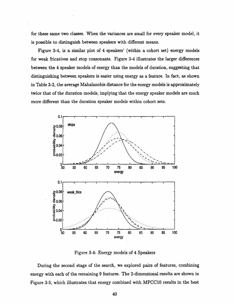
for these same two classes. When the variances are small for every speaker model, it
is possible to distinguish between speakers with different means.
Figure 3-4, is a similar plot of 4 speakers' (within a cohort set) energy models
for weak fricatives and stop consonants. Figure 3-4 illustrates the larger differences
between the 4 speaker models of energy than the models of duration, suggesting that
distinguishing between speakers is easier using energy as a feature. In fact, as shown
in Table 3-2, the average Mahalanobis distance for the energy models is approximately
twice that of the duration models, implying that the energy speaker models are much
more different than the duration speaker models within cohort sets.
55 60 65 70 75energy
80 85 90 95
energy
Figure 3-4: Energy models of 4 Speakers
During the second stage of the search, we explored pairs of features, combining
energy with each of the remaining 9 features. The 2-dimensional results are shown in
Figure 3-5, which illustrates that energy combined with MFCC10 results in the best
0.1
>0.08
" 0.06
- 0.02
05
Sstops
.IN
.- --
0

Feature Mahalanobis DistanceDuration 0.479Energy 0.926
Table 3-2: Average Mahalanobis Distances for 4 Speakers' Duration and EnergyModels
speaker verification performance, according to our distance measure. Furthermore,
there is a noticeable improvement in performance by the addition of another mea-
surement to the feature set, since the distances are smaller for the 2-dimensional sets
than for individual measurements. The performance improvement suggests that the
additional features carry further speaker-specific information. Also, the dimension of
the feature set is small enough that model parameters can be sufficiently estimated
from the 8 training utterances available per speaker.
Distances of Two-DimensionaFFeatures
60 65
Figure 3-5: Distances for 2-Dimensional Feature Sets
energymfcc6 (57.76)
energy_mfcc2 (59.06)
energyFO (60.72)
40 45 50 55Distance
erenergymfcclO (52.72)
energylmfcc3 (53.78)
energymfcc5 (54.36)
energymfccl4 (54.77)
energy mfcc8 (55.64)
energymfcc9 (55.68)
I I l I. i

During the third stage of the search, energy and MFCC10 were combined with
the 8 remaining measurements. The 3-dimensional results are shown in Figure 3-
6, which illustrates that the best 3-dimensional feature set is energy combined with
MFCC10 and MFCC5. We continued our feature search, since performance continued
to significantly improve, and accumulated dimensions to the feature vector in the
manner illustrated above. The results for 4 and 5-dimensional feature sets, along
with the numerical results of stages 2-7, are given in appendix C.
Distances of Three-Dimensional Features
energymfccl0 5 (43.04)
energy3mfcc10U6 (43.87)
energymfcc10_9 (44.13)
energymfcc10_14 (47.23)
energymfccl0O8 (48.49)
energy mfcclO_3 (49.20)
energy_mfcclO_FO (50.25)
energy.mfccl0_2 (52.39)
25 30 35 40 45 50 55 60Distance
Figure 3-6: Distances for 3-Dimensional Feature Sets
The 5-dimensional feature set that resulted in the best speaker verification perfor-
mance included energy, MFCC10, MFCC5, MFCC8, and MFCC6. These measure-
ments were then combined with each of the 5 remaining features. The six-dimensional
results are shown in Figure 3-7, which illustrates that the best 6-dimensional feature
set consists of energy, MFCC10, MFCC5, MFCC8, MFCC6, and MFCC14.
:

Distances of Six-Dimensional Features
energy_mfccl _5_8_6_14 (31.28)
energy_mfcc10_5_8_6_3 (31.39)
energy_mfcc10_5_8_6_9 (33.92)
energy_mfcc10_5_8_6_2 (34.01)
energy_mfccl0_5_8_6_FO (35.40)
10 15 20 25 30 35 40 45Distance
Figure 3-7: Distances for 6-Dimensional Feature Sets
I I i I I I
Next, we combined the 7-dimensional features sets to see if additional features
improved performance over the best set of 6 features found above. The results for the
7-dimensional sets are illustrated in Figure 3-8, which shows that all 7-dimensional
feature sets perform worse than the best 6-dimensional feature set. To observe
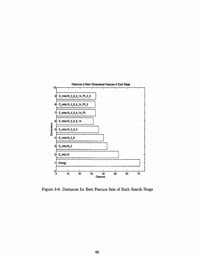
whether performance continued to degrade as features accumulated, we formed 8
and 9-dimensional feature sets. These sets were formed by adding FO and MFCC9 to
the best 7-dimensional feature set.
Figure 3-9 shows the results for the 8 and 9-dimensional feature sets, along with
the best results of each stage of the search. As illustrated in Figure 3-9, speaker
verification performance initially improves as more measurements are added to the
feature set, because the additional features contribute further speaker-specific infor-
mation. Also, there are sufficient amounts of training data to accurately estimate
the model parameters. However, adding features eventually degrades performance,
presumably because not enough training data is available to accurately estimate the
model parameters.
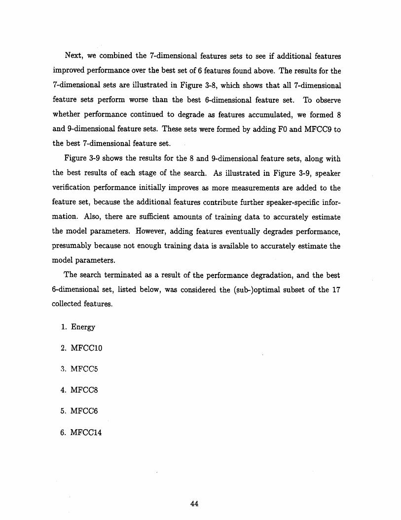
The search terminated as a result of the performance degradation, and the best
6-dimensional set, listed below, was considered the (sub-)optimal subset of the 17
collected features.
1. Energy
2. MFCC10
3. MFCC5
4. MFCC8
5. MFCC6
6. MFCC14
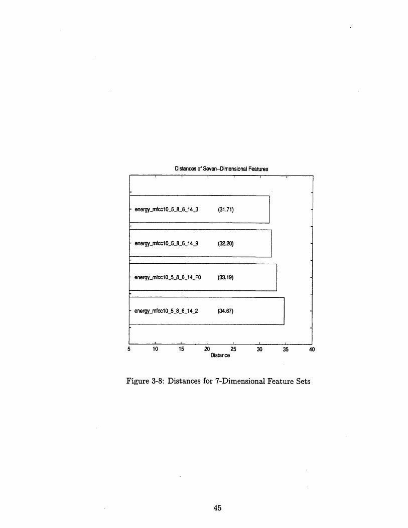
Distances of Seven-Dimensional FeaturesI i I I
energy_mfcc10_5_8_6_14_3 (31.71)
energy mfccl0_5_8_6_14 9 (32.20)
energymfcc 10._583__14_FO (33.19)
energymfccl0_5_8_6_14_2 (34.67)5 10 5 20 25 30 35 4
5 10 15 20 25 30 35 40Distance
Figure 3-8: Distances for 7-Dimensional Feature Sets
-
-
-
-
Distances of Best-Dimensional Features of Each Stage
- E_mfccl0_5_8_6_14_FO_3_9j
- Emfccl0_5_8_6_14_FO_3
- Emfcc10_5_8_6_14_FO
- E_mfcc10_5_8_6_14
- E mfcc10_5_8_6
- EmfcclO_ 5_8
- E mfccl0.5
-Emfccl0
- Energy
0 10 20 30 40Distance
50 60 70
Figure 3-9: Distances for Best Feature Sets of Each Search Stage
1 %
||
.d
3.3.2 Results Using 80 Speakers
The (sub-)optimal 6-dimensional feature set found using 168 test speakers should
be independent of the user population. To ensure that the feature search does not
produce significantly different results using another set of speakers, we conducted
an identical search using a set of 80 different users. The 80 speakers are a subset
of TIMIT's NIST-train set. This speaker set does not contain any speakers in the
original test set of 168 speakers. However, the 80 speakers have the same ratio of
males to females (2 to 1) as the first test set.
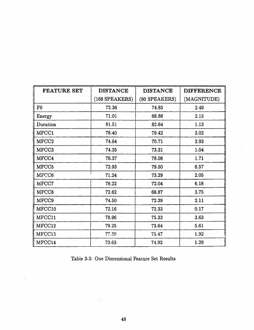
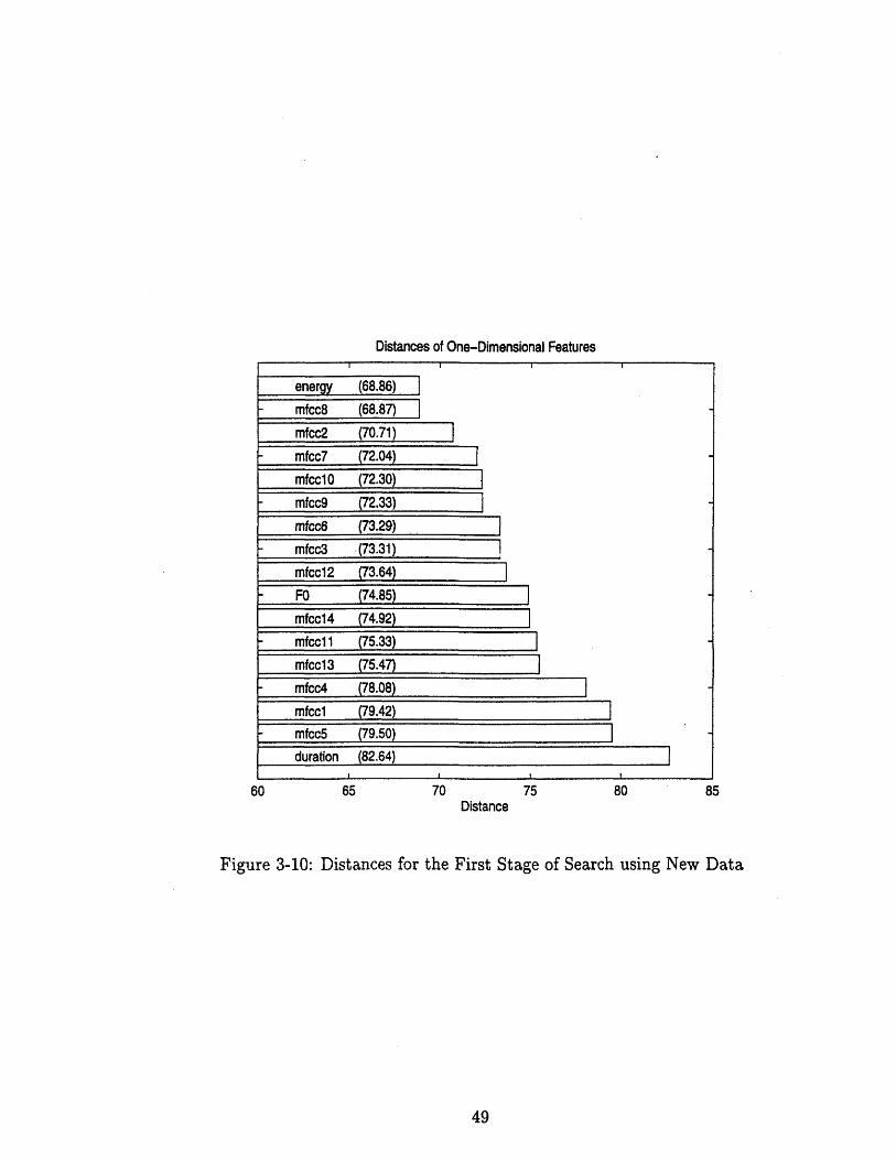
As before, we began the search by testing individual features from the initial
pool of 17 measurements. Table 3-3 and Figure 3-10 illustrate the results of the
first stage of the search. The results are similar to those obtained previously in the
first stage. Specifically, 8 out of the top 10 features from this search are included
in the top 10 features from the first search. However, the rankings of most features
changed. Unlike the first search, most of the 17 features in this search result in
similar performances and show potential to be useful features for speaker verification.
However, to replicate our search experiments, we still eliminated. 7 features and kept
the top 10 measurements for the remaining stages of the search. The top ranking
features still consisted of energy, FO, and the higher order MFCCs, with the exception
of the highly ranked MFCC2. As before, energy performed the best, and duration
performed the worst.
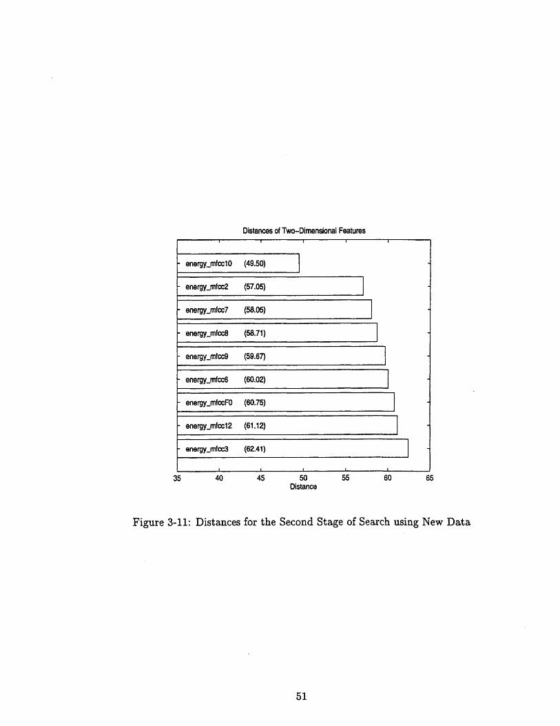
Since energy is still the best 1-dimensional feature, it was combined with the
remaining 9 of the top 10 features. These 2-dimensional sets were evaluated, and
performance results are given in Table 3-4. Figure 3-11 shows that the best pair of
features is energy and MFCC10, which is the same top performing 2-dimensional set
of the first search.
Due to time constraints, we terminated the search at this stage. However, we
believe that the performances of features have not significantly changed by testing
on a new set of speakers. The differences in the performances of some features are
presumably due to the fact that the new set is half the size of the former test set of
FEATURE SET DISTANCE DISTANCE DIFFERENCE
(168 SPEAKERS) (80 SPEAKERS) (MAGNITUDE)
FO 72.36 74.85 2.49
Energy 71.01 68.86 2.15
Duration 81.51 82.64 1.13
MFCC1 76.40 79.42 3.02
MFCC2 74.64 70.71 3.93
MFCC3 74.35 73.31 1.04
MFCC4 76.37 78.08 1.71
MFCC5 72.93 79.50 6.57
MFCC6 71.24 73.29 2.05
MFCC7 78.22 72.04 6.18
MFCC8 72.62 68.87 3.75
MFCC9 74.50 72.39 2.11
MFCC10 72.16 72.33 0.17
MFCC11 78.96 75.33 3.63
MFCC12 79.25 73.64 5.61
MFCC13 77.39 75.47 1.92
MFCC14 73.63 74.92 1.29
Table 3-3: One Dimensional Feature Set Results
Distances of One-Dimensional Features
energy (68.86)-Imfcc8 (68.87)m 2 of /7n 71\
mfcc7 (72.04)mfccl0 (72.30)-mfcc9 (72.33)mfcc6 (73.29)mfcc3 (73.31)
mfccl2 (73.64)-FO (74.85)
mfccl4 (74.92)
mfccl 1 (75.33)
mfccl3 (75.47)mfcc4 (78.08)
mfccl (79.42)mfcc5 (79.50)
duration (82.64)
Distance
Figure 3-10: Distances for the First Stage of Search using New Data
I

168 speakers.
FEATURE SET DISTANCE DISTANCE DIFFERENCE
(168 SPEAKERS) (80 SPEAKERS) (MAGNITUDE)
Energy .MFCC8 55.64 58.71 3.07
EnergyMFCC2 59.06 57.05 2.01
EnergyMFCC7 - 58.05 -
EnergyMFCC10 52.72 49.50 3.22
EnergyMFCC9 55.68 59.67 3.99
EnergyMFCC6 57.76 60.02 2.26
EnergyMFCC3 53.78 65.96 12.18
EnergyMFCC12 - 57.80 -
EnergyFO 60.72 53.95 6.77
Table 3-4: Two Dimensional Feature Set Results
3.4 System Performance
As mentioned in section 2.7.1, computation during testing is reduced by only scoring
test data against the purported speaker's model and models of the purported speaker's
cohort set, as opposed to all speaker models in the system. This technique is based on
the assumption that speaker models outside of the cohort set will not adversely affect
speaker verification performance. Since these outliers are considered too different
from the purported speaker, their models are expected to match the test data poorly
compared to the speaker models within the cohort set. If this is the case, the ROC
curves corresponding to performance using all speakers during testing can be obtained
from the ROC curves using only cohort sets during testing, via normalization. The
normalization divides the number of false acceptances obtained for a feature set, using
for each speaker only the S speakers in his/her cohort set as impostors, by the number
of possible false acceptances when all the remaining 167 speakers pose as impostors
for each speaker (168 speakers x 167 impostors).
Distances of Two-Dimensional Features
- energymfcclO0 (49.50)
- energymfcc2 (57.05)
energy-mfcc7 (58.05)
energymfcc8 (58.71)
energy-mfcc9 (59.67)
-energy-mfcc6 (60.02)
energy_mfccFO (60.75)
energymfccl2 (61.12)
energymfcc3 (62.41)
II f I f
35 40 45 50Distance
55 60 65
Figure 3-11: Distances for the Second Stage of Search using New Data
In both searches described above, we used a cohort set size of 14. We normalized
the results for the optimal 6-dimensional feature set found using 168 test speakers, and
obtained a performance of 0% false rejection of true users and 6.54% false acceptance
of impostors. To verify whether these normalized approximations are reasonably close
to performance using all speakers during testing, we repeated the experiment on the
optimal feature set using all 168 speakers during testing. Figure 3-12 plots the ROC
curve for the optimal feature set obtained using all speakers as impostors, and the
normalized ROC curve obtained using 14 impostors per speaker. As Figure 3-12
illustrates, the normalized results are very similar to the results obtained using all
speakers during testing (0% false rejection of true users and 4.85% false acceptance
of impostors).
The curves do not match exactly, suggesting that the ranks of the speaker model's
score and cohort speaker models' scores were not always the top 15 of 168 scores. In
fact, the rank of the true speaker's model within the 15 cohort scores is always greater
than or equal to the rank of the same model's score within 168 scores. This results in
smaller rates of FR and FA for each rank threshold for the normalized cohort results
(•etter perfocrnzce). IiHo ,er, the cLrves aie ~if•ar enough that usirg coort sets
to reduce computation during testing appears to have no significant adverse affects
on speaker verification performance.
3.5 Performance Comparison
In order to evaluate the advantages and disadvantages of our approach to the speaker
verification task, it is necessary to compare our system's performance and design to
those of other systems. Often, it is difficult to compare systems unequivocally because
the data used to evaluate the systems and the evaluation methods may differ. In order
to make somewhat meaningful comparisons, we compare our system with two other
systems, described below, that also use the TIMIT corpus.

I- m mhnrte- 14I0rCOnoI[s
5 10 15 20 25 30False Acceptance %
35 40 45 50
Figure 3-12: ROC Curves Using 168 Speakers and Normalizing RIesiuts Using 14Cohorts
c30
6=25
20• 20U.
'1
'.1'I
SIiii
1t
I I I I I I I
I ~I"~T~T i
3.5.1 HMM Approach
A state-of-the-art HMM speech recognition system, built by Lamel and Gauvain [19],
was recently modified for speaker recognition. The system extracts frame-based
acoustic features, which include 15 MFCCs, first derivatives of the MFCCs, energy,
and the first and second derivative of energy. During training, 8 utterances (2 SA,
3 SX and 3 SI) were used to build speaker models. To develop the speaker models,
a general speaker-independent model of 40 phonetic classes was trained on the 462
speakers in the TIMIT NIST-train set. This model then served as a seed model to
be used to adapt, via the maximum a posteriori procedure (MAP discussed in sec-
tion 4.2.5), each speaker-specific model. During adaptation, the speaker models were
modified to represent 31 broad phonetic classes, rather than 40. During testing, 168
speakers from TIMIT's NIST-test and NTST-dev sets were evaluated. The 168 speaker
models were combined in parallel into one large HMM, which was used to recognize
the test speech of the remaining 2 SX sentences of each user. To classify speakers,
the system used the phone-based acoustic likelihoods produced by the HMM on the
set of 31 broad class models. The speaker model with the highest acoustic likelihood
was identified as the speaker.
Lamel and Gauvain reported 98.8% speaker identification accuracy using 1 test
utterance and 100% accuracy using 2 test utterances. Since we perform mini-speaker
identification tests in our system, these HMM results can be compared to our results
when we use all speakers during testing. Essentially, if we were to convert the HMM
speaker identification system above into a speaker verification system that implements
our decision algorithm, the system achieves 0% false rejection of true users with 0%
false acceptance of impostors.
Lamel's system is evaluated on the same set of 168 test speakers as our test
set. However, the sentences used during testing are two SX, whereas we test each
speaker using the 2 SA utterances. Unlike the SA sentences, the SX sentences are
each repeated 7 times by 7 different speakers. Thus, a test sentence may be included
in the training set, suggesting that the system may have seen the same sequence

of phones (spoken by different speakers) in both testing and training stages. As a
result, better performance may result over a system which tests completely different
orthography than the training data.
3.5.2 Neural Network Approach
Another competitive system that uses the TIMIT corpus is a neural network-based
speaker identification system built by Younes Bennani [2]. The system computes 16
frame-based cepstral coefficients derived from linear prediction coefficients (LPCs).
Before training, acoustic vectors computed from the 5 SX utterances for 102 speak-
ers were grouped together into homogeneous classes, via a non-supervised k-means
algorithm. 2 Each of the 102 test speakers was then assigned to the class to which
the majority of the speaker's acoustic vectors belonged. During training, a typology
detector and a set of expert modules (neural networks), which discriminate between
speakers of the same typology, were developed. During testing, 102 speakers were
evaluated using 3 SI sentences. To classify speakers, a score computed from a weight-
ing of scores of the typology detection module with those of the expert modules is
used.
Bennani's neural network system achieved a performance of 100% identification
accuracy. Again, if the system implements the speaker verification decision algorithm
we use, it would result in 0% false rejection of true users with 0% false acceptance
of impostors. Table 3-5 summarizes the design and performance of the two systems
discussed above and of our system.
3.5.3 Performance versus Computational Efficiency
As illustrated above, there are high performance speaker verification systems that are
evaluated on the TIMIT corpus. Although both of the systems described above use
TIMIT, they evaluate the systems on either a different set of sentences, or a different
2Exact speaker set is not reported in reference paper, but the set is not the same as our test setof 168 speakers.
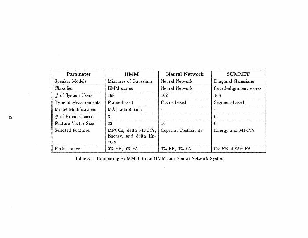
Parameter HMM Neural Network SUMMIT
Speaker Models Mixtures of Gaussians Neural Network Diagonal Gaussians
Classifier HMM scores Neural Network forced-alignment scores
# of System Users 168 102 168
Type of Measurements Frame-based Frame-based Segment-based
Model Modifications MAP adaptation -
# of Broad Classes 31 - 6
Feature Vector Size 32 16 6
Selected Features MFCCs, delta MFCCs, Cepstral Coefficients Energy and MFCCsEnergy, and dkelta En-ergy
Performance 0% FR, 0% FA 0% FR, 0% FA 0% FR, 4.85% FA
Table 3-5: Comparing SUMMIT to an HMM and Neural Network System
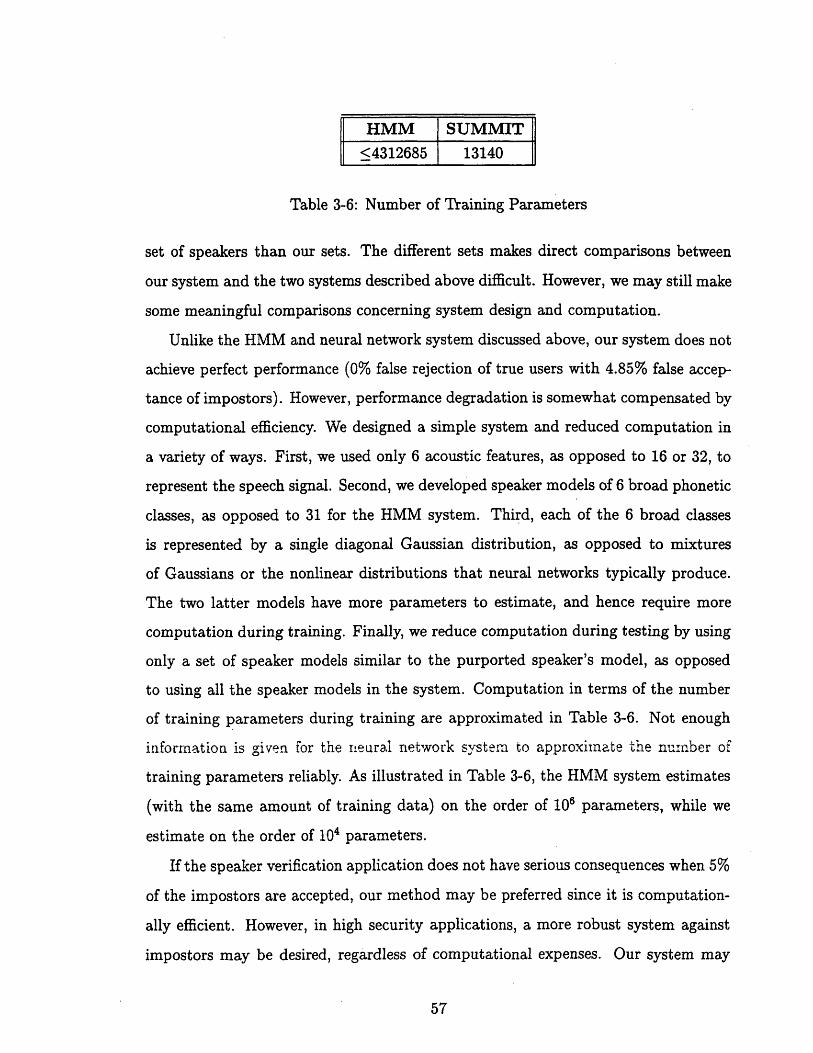
HMM SUMMIT<4312685 13140
Table 3-6: Number of Training Parameters
set of speakers than our sets. The different sets makes direct comparisons between
our system and the two systems described above difficult. However, we may still make
some meaningful comparisons concerning system design and computation.
Unlike the HMM and neural network system discussed above, our system does not
achieve perfect performance (0% false rejection of true users with 4.85% false accep-
tance of impostors). However, performance degradation is somewhat compensated by
computational efficiency. We designed a simple system and reduced computation in
a variety of ways. First, we used only 6 acoustic features, as opposed to 16 or 32, to
represent the speech signal. Second, we developed speaker models of 6 broad phonetic
classes, as opposed to 31 for the HMM system. Third, each of the 6 broad classes
is represented by a single diagonal Gaussian distribution, as opposed to mixtures
of Gaussians or the nonlinear distributions that neural networks typically produce.
The two latter models have more parameters to estimate, and hence require more
computation during training. Finally, we reduce computation during testing by using
only a set of speaker models similar to the purported speaker's model, as opposed
to using all the speaker models in the system. Computation in terms of the number
of training parameters during training are approximated in Table 3-6. Not enough
i.nformrnation is given for the neura.l network system to approximate the number of
training parameters reliably. As illustrated in Table 3-6, the HMM system estimates
(with the same amount of training data) on the order of 106 parameters, while we
estimate on the order of 104 parameters.
If the speaker verification application does not have serious consequences when 5%
of the impostors are accepted, our method may be preferred since it is computation-
ally efficient. However, in high security applications, a more robust system against
impostors may be desired, regardless of computational expenses. Our system may
improve in performance and robustness by better modeling of features, and/or better
selections of broad classes, for example. Such future work is discussed in the final
chapter.

Chapter 4
Conclusions & Future Work
4.1 Summary
This thesis attempted to achieve two goals. The first was to build a competitive
segment-based speaker verification system, and the second goal was to build a com-
putationally efficient system. Often, these goals cannot be achieved simultaneously.
Systems that achieve 0% error may not be computationally efficient. Below, we briefly
discuss how we significantly reduced computation while maintaining good speaker
verification performance.
As described in section 3.2, our system achieves a performance of 0% false re-
jection of true users and 4.85% false acceptance of impostors. Although the false
acceptance rate is not 0%, we significantly reduced computation in many ways. As
previously mentioned, the system uses a small number of features, a small number
of phonetic models per speaker, few model parameters, and few competing speakers
during testing. We believe that the system is able to achieve good performance with a
simple design because we treated speech as a concatenation of segments, rather than
frames. Past observations show that speech segments carry speaker-specific informa-
tion. Therefore, by considering the speech signal as a concatenation of phone-size
units, we capitalized on measurements for such units more readily.
4.2 Future Work
In this section, we discuss possible future work in connection with our research. This
work includes exploring robustness issues, conducting an exhaustive search for opti-
mal acoustic features, selecting broad classes based on acoustic criteria, representing
features with more complex distributions, and adapting speaker models. Finally,
we plan to incorporate our speaker verification system into a web-based information
access system called GALAXY.
4.2.1 Robustness Issues
An important future topic to investigate is the robustness of the system in various
acoustic environments. Although we achieved good speaker verification performance
on the TIMIT corpus, the training environment matched the testing environment.
In reality, these two environments usually differ. For example, training data may be
collected in a quiet environment over a microphone, while test data are transmitted
through a noisier environment over a telephone. The noisy environment and lim-
ited bandwidth cause feature statistics to change; thus test data are mis-matched to
trained models.
To appreciate the magnitude of the degradation in performance due to mis-
matched environments, we evaluated our system using speaker models trained on
TIMIT and tested on NTIMIT. As mentioned in section 2.2, NTIMIT is TIMIT
transmitted over a telephone network. Figure 4-1 gives an indication of how SV per-
fornmance degrades when testing on mis-matched da-a. To achieve 0% false rejection
of true users, the system falsely accepts 48.27% of impostors on NTIMIT test data,
suggesting the necessity to design a robust system for noisy environments. Perhaps
an algorithm could be adopted to re-estimate the speaker model parameters trained
on clean speech to better fit noisy test data. Alternatively, it may be necessary to
search for better acoustic features for the noisy environment.
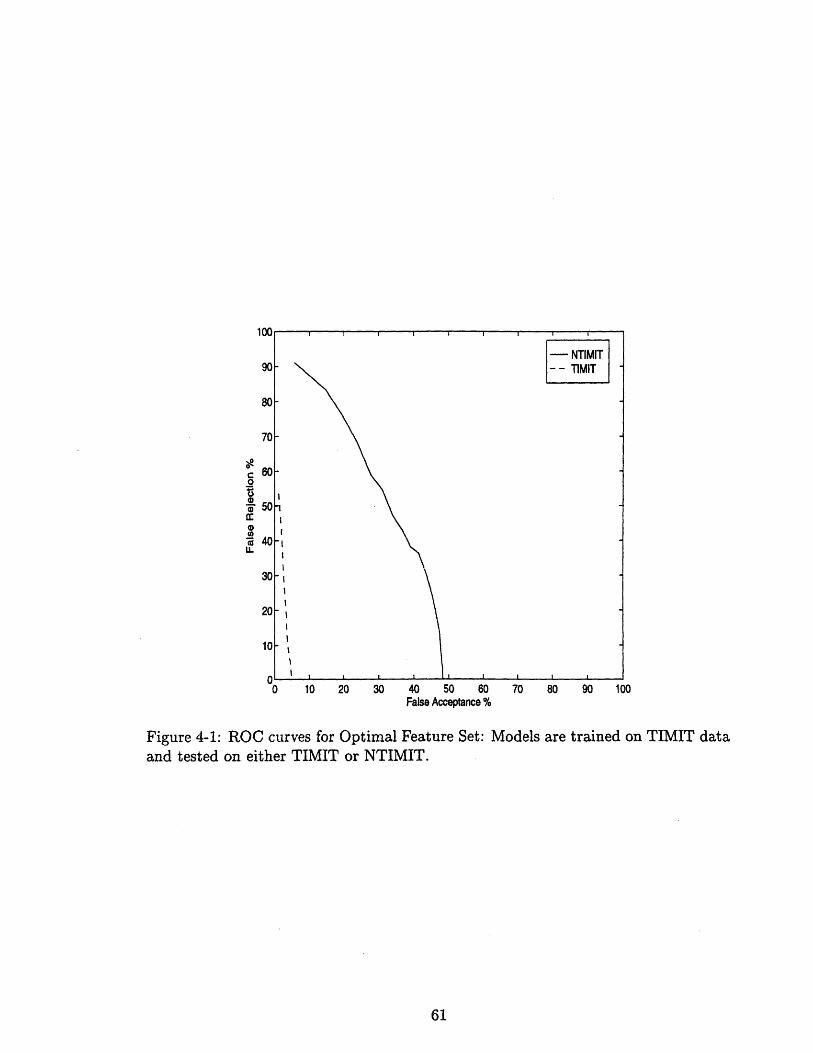
NTIM I I
NTIMIT
0 10 20 30 40 50 60False Acceptance %
Figure 4-1: ROC curves for Optimal Feature Set: Moand tested on either TIMIT or NTIMIT.
70 80 90 100
dels are trained on TIMIT data
5
50
Z 40U.
I_K i
nL , =, I I i I i I I I I
I-- 1MIT I
I I I I
U-
I I I Iti
4.2.2 Exhaustive Search for Robust Features
In this thesis, we conducted a greedy search with pruning for a (sub)-optimal set of
acoustic features. Since we did not explore all possible feature sets formed from the
17 selected measurements, we do not know whether or not the best feature set found
from the greedy search is optimal. To ensure that a feature set formed from a pool of
measurements is optimal, an exhaustive search without pruning should be conducted.
Optimality may be more important in domains where performance degrades signifi-
cantly with different feature sets, as in noisy environments. As illustrated above, our
(sub)-optimal feature set results in good performance when train and test environ-
ments are clean. However, performance degrades significantly with the same feature
set, when testing in a noisy domain.
In the future, we plan to use a program called SAILS to help us extract optimal and
robust features. SAILS [31] was originally used to extract optimal acoustic attributes
that signify phonetic contrasts for speech recognition. It allows the user to vary
parameters such as frequency range and time interval for measuring any set of features
for selected speakers' phonemes, and their left and right phonetic contexts. For
example, if the algorithm explores MFCCs, SAILS finds optimal places to start and
end measuring the coefficients (SAILS specifies a range in the segment to compute
over, such as 30%-70% of the segment), as well as which coefficients best discriminate
between speakers' phonemes.
4.2.3 Feature-Motivated Broad Class Selections
As observed in this thesis, our selection of the broad manner classes affected the
performance of various features, especially duration. In the past, duration has been
proven to be robust and speaker-specific [41]. However, the classes we selected did not
reflect different duration characteristics. As a result, the variances of duration were
large for all speakers models, and the performance scores using duration ranked last
in the scores for the 1-dimensional stage for both searches conducted. Thus, duration
was eliminated in the search for optimal features.
In order to prevent disregarding potentially useful features for speaker verifica-
tion, and to ensure that each broad class has small variances, we plan to select broad
classes by using an unsupervised clustering algorithm. Unsupervised clustering algo-
rithms, such as the K-means algorithm, group phones into classes based on acoustic
characteristics. Thus, unlike the manner classes, each broad class should have similar
acoustic statistics. As a result, the speaker models will have small variances for all
features, which makes distinguishing between speakers easier than if the models have
large variances. In turn, we hope to improve speaker verification performance.
4.2.4 Representing Features With More Complex Distribu-
tions
Future work also includes exploring more complex feature distributions than diagonal
Gaussians. We chose to represent the broad class acoustic statistics with diagonal
Gaussians, which have few parameters to train, to reduce computation. As a result we
traded model accuracy for computation. Essentially, we forced the acoustic features
for each class to be represented by a mean vector and a diagonal covariance matrix,
which assumes that the features are uncorrelated random variables. Features may
be more accurately modeled with mixtures of diagonal Gaussians, or full covariance
Gaussians. Given enough data, more complex models may improve speaker verifica-
tion performance. However, computation increases, since complex models have many
parameters to estimate during training.
4.2.5 Adaptation of Models
Often, little training data are available per speaker. As a result the speaker models
estimated from the data are not reliable. Ideally, one would like to obtain accurate
models from little training data so that users will not be required to speak many
utterances before being able to use the system. To reliably represent speakers with
little training data, many investigators apply adaptation techniques to the speaker
models. Specifically, the means, variances, and a priori broad class probabilities are
typically adapted from the statistics of a well-trained speaker-independent model.
As a first attempt to observe performance effects due to adaptation of speaker
models, we modified the a priori class probabilities of each speaker model. Specifically,
we first trained a speaker-independent (SI) model using data from the 462 speakers'
data from the NIST-train set of TIMIT. These estimates were then adapted to each
speaker model. This simple technique forced the a priori estimates to be accurate and
consistent across all speakers. The a priori class probabilities should be independent
of speakers since the probability of observing a particular broad class in a segment is
dependent only on the lexicon in the corpus.
Figure 4-2 illustrates the performance, before and after applying our adaptation
method, evaluated on the original 168 test speakers using the optimal 6-dimensional
feature set. As shown in the figure, there is no significant improvement in performance
when we only adapt the a priori class probabilities. Perhaps the a priori estimates
did not differ significantly from speaker to speaker before adaptation, resulting in
little performance differences. The insignificant improvement after adaptation of the
a prioris suggests that more complex adaptation techniques that modify means and
variances are required to improve the speaker models, and in turn improve speaker
verification performance.
In the future, we plan to implement the maximum a-posteriori probability (MAP)
adaptation procedure, a common method for adapting all the statistics of models.
MAP provides a way to incorporate prior information into the estimation process, by
assuming an a-priori distribution of the parameters that are being estimated. Details
on the MAP technique can be found in [39, 23].
4.2.6 Incorporating i~ito GALAXY
Finally, we plan to incorporate our speaker verification system into the GALAXY
conversational system [13]. GALAXY is a system currently under development in our
group that enables information access using spoken dialogue. Presently, GALAXY
can access the information sources on the Internet via speech for four applications:
weather reports, airline travel information, automobile sales information, and the
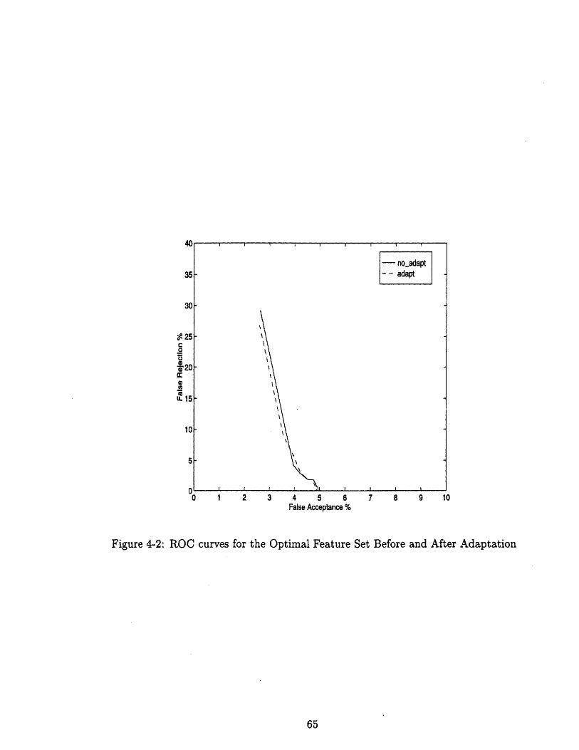
25
?20
LL 15
10
5
0 1 2
rI I
- noadaptS adapt
3 4 5 6False Acceptance %
7 8 9 10
Figure 4-2: ROC curves for the Optimal Feature Set Before and After Adaptation
II I i i , i ill i , f i I

Boston city guide.
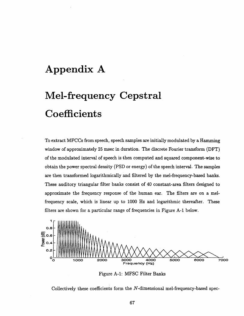
Appendix A
Mel-frequency Cepstral
Coefficients
To extract MFCCs from speech, speech samples are initially modulated by a Hamming
window of approximately 25 msec in duration. The discrete Fourier transform (DFT)
of the modulated interval of speech is then computed and squared component-wise to
obtain the power spectral density (PSD or energy) of the speech interval. The samples
are then transformed logarithmically and filtered by the mel-frequency-based banks.
These auditory triangular filter banks consist of 40 constant-area filters designed to
approximate the frequency response of the human ear. The filters are on a mel-
frequency scale, which is linear up to 1000 Hz and logarithmic thereafter. These
filters are shown for a particular range of frequencies in Figure A-i below.
O 1000 2000 3000 4000 5000 6000Frequency (Hz)
Figure A-i: MFSC Filter Banks
Collectively these coefficients form the N-dimensional mel-frequency-based spec-
0.8
~ 0.6
0.4
0.2
7000
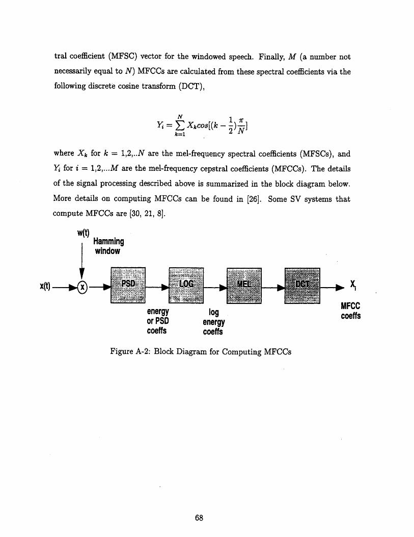
tral coefficient (MFSC) vector for the windowed speech. Finally, M (a number not
necessarily equal to N) MFCCs are calculated from these spectral coefficients via the
following discrete cosine transform (DCT),
N
1 = Z xkcos[(k - ) ]k=12
where Xk for k = 1,2,..N are the mel-frequency spectral coefficients (MFSCs), and
Y, for i = 1,2,...M are the mel-frequency cepstral coefficients (MFCCs). The details
of the signal processing described above is summarized in the block diagram below.
More details on computing MFCCs can be found in [26]. Some SV systems that
compute MFCCs are [30, 21, 8].
w(t)iUrnmminn
MFCCcoeffsenergy log
or PSD energycoeffs coeffs
Figure A-2: Block Diagram for Computing MFCCs
X(t) -
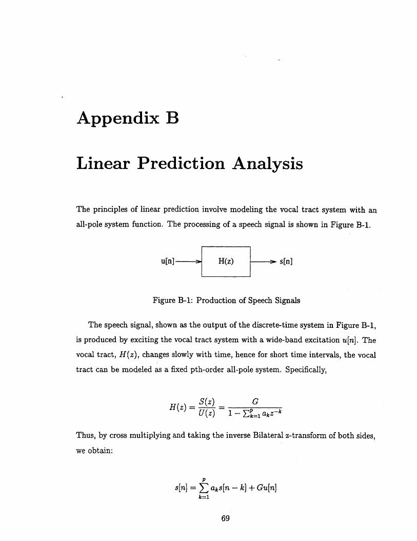
Appendix B
Linear Prediction Analysis
The principles of linear prediction involve modeling the vocal tract system with an
all-pole system function. The processing of a speech signal is shown in Figure B-1.
u[n] = H(z) s[n]
Figure B-1: Production of Speech Signals
The speech signal, shown as the output of the discrete-time system in Figure B-l,
is produced by exciting the vocal tract system with a wide-band excitation u[n]. The
vocal tract, H(z), changes slowly with time, hence for short time intervals, the vocal
tract can be modeled as a fixed pth-order all-pole system. Specifically,
SH(z) (z) GU(z) 1 - EP=z az -k
Thus, by cross multiplying and taking the inverse Bilateral z-transform of both sides,
we obtain:
p
s[n] = aks[n - k] + Gu[n]k=1

The goal of linear prediction analysis is to estimate the ak's and G from s[n]. The
predicted signal is defined as:
P
[n]= Laks[n -k]k=1
which leaves a residual error e[n] = s[n] - 9[n] ~ Gu[n] (this is approximately true
when the estimates ak's are very good). The ak's are chosen to minimize the residual
error. SV systems that use LPCs for acoustic features are [18, 42, 3]. For a tutorial
on LPC analysis, refer to [22].
B.1 Estimation of Fundamental Frequency
There are many methods to approximate FO, such as cepstral analysis and LPC
analysis. We describe the approximation of FO using linear prediction analysis below.
Refer to [29] for the method of approximating FO from cepstral coefficients. In order
to estimate the fundamental frequency using LPC analysis, the autocorrelation of the
error function is computed. During a fixed time interval of the speech signal, si[n] can
be assumed to be N points in length, which makes the autocorrelation function of
the error, Re[kl], a finite sum for each n. Specifically,
N-1-kRe[k] = Z einje[n + k]
n=1
When the speech signal is voiced, u[n] is assumed a train of narrow glottal pulses.
The signal is then windowed over an interval, and a few of the pulses remain in the
interval if the window is larger than a few pulse periods. Note that the fundamental
frequency is simply the reciprocal of the fundamental period of the pulses. The
autocorrelation function of the residual error exhibits local maxima where the pulses
occur. An example of the error autocorrelation function for a voiced time interval
is illustrated in Figure B-2. These functions are plotted for every frame, and the
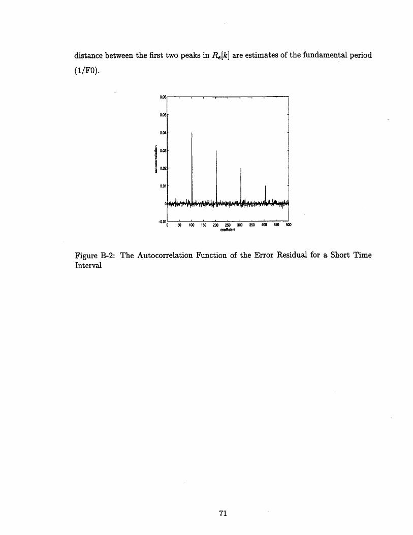
distance between the first two peaks in Re[k] are estimates of the fundamental period
(1/FO).
-40 50 100 150 200 250 300 350 400 450
coeffident
Figure B-2: The Autocorrelation Function of the Error Residual for aInterval
Short Time
U.ULiI r I
0~jh I, ,
u| .......
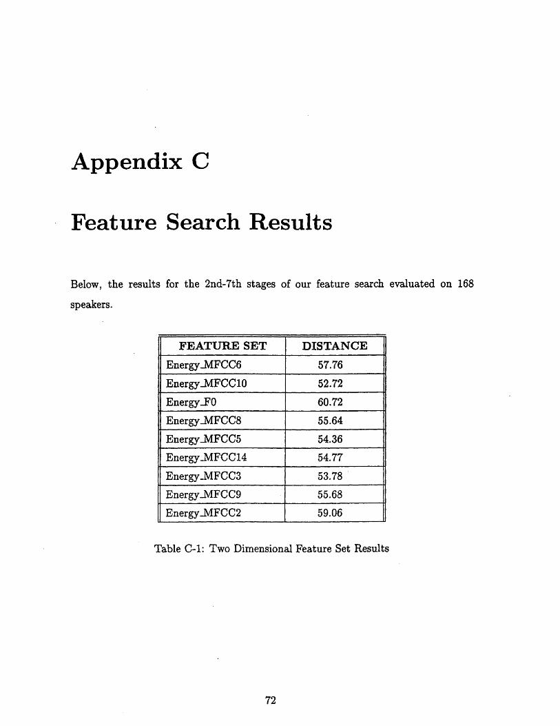
Appendix C
Feature Search Results
Below, the results for the 2nd-7th stages of our feature search evaluated on 168
speakers.
FEATURE SET DISTANCE
Energy.MFCC6 57.76
EnergyMFCC10 52.72
EnergyFO 60.72
Energy_MFCC8 55.64
Energy.MFCC5 54.36
EnergyMFCC14 54.77
EnergyMFCC3 53.78
EnergyMVIFCC9 55.68
Energy.MFCC2 59.06
Table C-1: Two Dimensional Feature Set Results
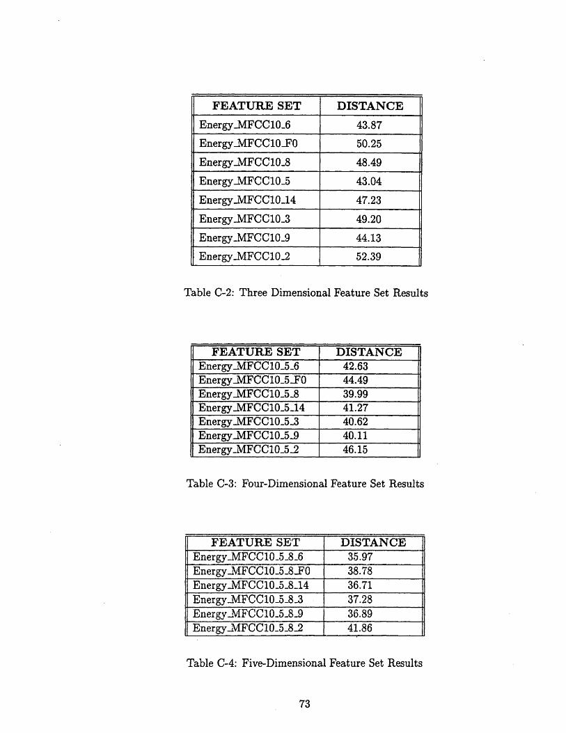
FEATURE SET DISTANCE
EnergyMFCC10_6 43.87
EnergyMFCC10.FO 50.25
EnergyMFCC10-8 48.49
EnergyMFCC10_5 43.04
Energy-MFCC10_14 47.23
EnergyMFCC10 3 49.20
EnergyMFCC10_9 44.13
EnergyMFCC10_2 52.39
Table C-2: Three Dimensional Feature Set Results
FEATURE SET DISTANCEEnergyMFCC 105-6 42.63EnergyJMFCC105.FO 44.49EnergyMFCC105-8 39.99Energy _MFCC10_5-14 41.27EnergyMFCC10O5_3 40.62EnergyiMFCC10_5-9 40.11Energy_MFCC10_5_2 46.15
Table C-3: Four-Dimensional Feature Set Results
FEATURE SET DISTANCEEnergyMFCC10_5_8_6 35.97Energy MFCC10-5-8FO 38.78Energy.MFCC10_5 _814 36.71EnergyMVIFCC10_5_8_3 37.28EnergyMFCC10-5-8-9 36.89EnergyMFCCl0_5O82 41.86
Table C-4: Five-Dimensional Feature Set Results
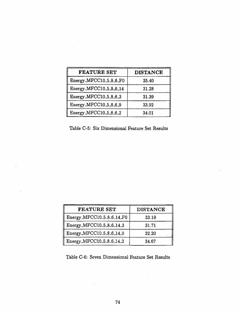
FEATURE SET DISTANCE
EnergyMFCC10_5.8 _6F0 35.40
EnergyMFCC105 8 _6_14 31.28
EnergyMFCC105_8 _6 3 31.39
Energy.MFCC105_8_6_-9 33.92
Energy MFCC10_5_8_6_2 34.01
Table C-5: Six Dimensional Feature Set Results
FEATURE SET DISTANCE
Energy MFCC10_5_8 _614_0 33.19
Energy•MFCC10_5 _86_14,3 31.71
Energy.MFCC10_5_8 _6_14_9 32.20
EnergyMFCC10_5_8_6_14_2 34.67
Table C-6: Seven Dimensional Feature Set Results
Bibliography
[1] B. Atal. Automatic speaker recognition based on pitch contours. JASA, 52:1687-
1697, 1972.
[2] Y. Bennani. Speaker identification through modular connectionist architecture:
evaluation on the timit database. In Proceedings of the 1992 International Con-
ference on Spoken Language Processing, pages 607-610, 1992.
[3] Y. Bennani and P. Gallinari. On the use of tddn-extracted features information
in talker identification. In Proceedings of the 1991 International Conference on
Acoustics, Speech, and Signal Processing, pages 385-388. IEEE, 1991.
[4] J. Campbell. Testing with he yoho cd-rom voice verification corpus. In Pro-
ceedings of the 1995 International Conference on Acoustics, Speech, and Signal
Processing, pages 341-344. IEEE, 1995.
[5] T. Cormen, C. Leiserson, and R. Rivest. Introduction to Algorithms. The MIT
Press, 1990.
[6] G. Doddington. Speaker recognition-identifying people by their voices. Proceed-
ings of the IEEE, 73(11):1651-1663, November 1985.
[7] G. Doddington and B. Secrest. An integrated pitch tracking algorithm for speech
systems. In Proceedings of the 1983 International Conference on Acoustics,
Speech, and Signal Processing, pages 1352-1355, 1983.

[8] K. Farrel and R. Mammone. Speaker identification using neural networks. In
Proceedings of the 1994 International Conference on Acoustics, Speech, and Sig-
nal Processing, pages 165-168. IEEE, 1994.
[9] D. Gaganelis. A novel approach to speaker verification. In Proceedings of the 1991
International Conference on Acoustics, Speech, and Signal Processing, pages 373-
376. IEEE, 1991.
[10] J. Garofolo, L. Lamel, W. Fisher, J. Fiscus, D. Pallett, and N. Dahlgren. Darpa
timit acoustic-phonetic continuous speech corpus cd-rom. In National Institute
of Standards and Technology, 1990.
[11] J. Glass. Finding acoustic regularities in speech: applications to phonetic recog-
nition. PhD thesis, Massachusetts Institute of Technology, 1988.
[12] J. Glass, J. Chang, and M. McCandless. A probabilistic framework for feature-
based speech recognition. In Proceedings of the 1996 International Conference
on Spoken Language Processing, 1996.
[13] D. Goddeau, E. Brill, J. Glass, C. Pao, M. Phillips, J. Polifroni, S. Seneff, and
V. Zue. Galaxy: A human-language interface to on-line travel information. In
Proceedings of the 1994 International Conference on Spoken Language Process-
ing, 1994.
[14] U. Goldstein. An Investigation of Vowel Formant Tracks for Purposes of Speaker
Identification. PhD thesis, Mvassachusetts Institute of Technology, 1975.
[15] S. Hangai and K. Miyauchi. Speaker identification based on multipulse excitation
and lpc vocal-tract model. In Proceedings of the 1990 International Conference
on Spoken Language Processing, pages 1269-1272, 1990.
[16] C. Jankowski, A. Kalyanswamy, S. Basson, and J. Spitz. N-timit:a phonetically
balanced, continuous speech, telephone bandwidth speech database. In ICAASP,
pages 109-112, 1990.
[17] C. Jankowski, T. Quatieri, and D. Reynolds. Measuring fine structure in speech:
Application to speaker identification. In Proceedings of the 1995 International
Conference on Acoustics, Speech, and Signal Processing, pages 325-328. IEEE,
1995.
[18] I. Jou, S. Lee, and M. Lin. A neural network based speaker verification sys-
tem. In Proceedings of the 1990 International Conference on Spoken Language
Processing, pages 1273-1276, 1990.
[19] L. Lamel. A phone-based approach to non-linguistic speech feature identification.
Computer Speech and Language, 9:87-103, 1995.
[20] R. Lippman. An introduction to computing with neural nets. IEEE ASSP
Magazine, 1987.
[21] M. Lund, C. Lee, and C. Lee. A distributed decision approach to speaker verifica-
tion. In Proceedings of the 1994 International Conference on Acoustics, Speech,
and Signal Processing, pages 141-144. IEEE, 1994.
[22] J. Makhoul. Linear prediction: A tutorial review. Proceedings of the IEEE,
63(4), April 1975.
[23] J. Makhoul, R. Schwartz, and G. Zavaliagkos. Adaptation algorithms for bbn's
phonetically tied mixture system. In ARPA SCSTW, pages 82-87, 1995.
[24] T. Matsui and S. Furui. A text independent speaker recognition method robust
against utterance variations. In Proceedings of the 1991 International Conference
on Acoustics, Speech, and Signal Processing, pages 377-380. IEEE, 1991.
[25] T. Matsui and S. Furui. Comparison of text-independent speaker recognition
methods using vq distortion and discrete/continuous hmms. IEEE Transactions
on Signal Processing, 2(157), 1992.
[26] H. Meng. The use of distinctive features for automatic speech recognition, 1991.
[27] J. Naik. Speaker verification:a tutorial. IEEE Communications Magazine, pages
42-47, January 1990.
[28] J. Oglesby and J. Mason. Radial basis function networks for speaker recognition.
In Proceedings of the 1991 International Conference on Acoustics, Speech, and
Signal Processing, pages 393-396. IEEE, 1991.
[29] A. Oppenheim and R. Schafer. Discrete- Time Signal Processing. PTR Prentice
Hall, Inc., 1989.
[30] E. Parris and M. Carey. Discriminative phonemes for speaker identification. In
Proceedings of the 1994 International Conference on Spoken Language Process-
ing, pages 1843-1846, 1994.
[31] M. Phillips and V. Zue. Automatic discovery of acoustic measurements for pho-
netic classification. In Proceedings of the 1992 International Conference on Spo-
ken Language Processing, pages 795-798, 1992.
[32] L. Rabiner. A tutorial on hidden markov models and selected applications in
speech recognition. Proceedings of the IEEE, 77(2):257-286, February 1989.
[33] L. Rabiner and B.H. Juang. Fundamentals of Speech Recognition. PTR Prentice
Hall, Inc., 1993.
[34] Rosenburg, DeLong, Lee, Juang, and Soong. The use of cohort normalized scores
for speaker verification. In Proceedings of the 1992 International Conference on
Spoken Language Processing, pages 599-602, 1992.
[35] A. Rosenburg, C. Lee, and S. Gokcen. Connected word talker verification using
whole word hidden markov models. In Proceedings of the 1991 International
Conference on Acoustics, Speech, and Signal Processing, pages 381-384. IEEE,
1991.
r26] L. Rudasi and S. Zahorian. Text-independent talker identification with neural
networks. In Proceedings of the 1991 International Conference on Acoustics,
Speech, and Signal Processing, pages 389-392. IEEE, 1991.
[37] M. Sambur. Speaker Recognition and Verification using Linear Prediction Anal-
ysis. PhD thesis, Massachusetts Institute of Technology, 1972.
[38] Y. Tohkura. A weighted cepstral distance measure for speech recognition. Com-
puter Speech and Language, 35:1414, 1987.
[39] H. Van Trees. Detection, Estimation, and Modulation Theory (Part I). John
Wiley and Sons, Inc., 1968.
[40] J. Wolf. Acoustic Measurements for Speaker Recognition. PhD thesis, Mas-
sachusetts Institute of Technology, 1969.
[41] B. Yegnanarayana, S. Wagh, and S. Rajendra. A speaker verification system
using prosodic features. In Proceedings of the 1994 International Conference on
Spoken Language Processing, pages 1867-1870, 1994.
[42] H. Yin and T. Zhou. Speaker recognition using static and dynamic cepstral
feature by a learning neural network. In Proceedings of the 1990 International
Conference on Spoken Language Processing, pages 1277-1280, 1990.
[43] V. Zue, M. Phillips, and S. Seneff. The mit summit speech recognition system: A
progress report. In Proceedings DARPA Speech and Natural Language Workshop,
pages 179-189, 1989.