a scheduling-based routing network architecture omar y. tahboub & javed i. khan multimedia &...
Post on 22-Dec-2015
214 views
TRANSCRIPT

A Scheduling-based Routing Network Architecture
Omar Y. Tahboub & Javed I. KhanMultimedia & Communication Networks Research Lab (MediaNet)
Kent State University

Outline Introduction
The Scheduling-based Routing Network Architecture
Case Study: An Institutional Remote Data Backup & Recovery Network
Performance Evaluation.
Conclusion and Future Work
Outline Introduction
The Scheduling-based Routing Network Architecture
Case Study: An Institutional Remote Data Backup & Recovery Network
Performance Evaluation.
Conclusion and Future Work

Introduction Bandwidth-intensity will be dominating aspect in future emergent Internet
applications.
Will pose network capacity demands beyond imagination reaching Gigabytes and yet Terabytes per day.
Internet2 [1] model will likely be the reference architectural model for the next generation high-performance networks.
The Internet2 Dynamic Circuit Networking (DCN) [2] will also be the key communication paradigm.
Multi Protocol Labeling Switching (MPLS) [3] play a central role massive data flow routing, switching and forwarding

Introduction
Finally, on the basis of the case study, we carried out a performance evaluation study: Demonstrated two simulation experiments. Compared the performance between the scheduled data backup transfer to the
conventional non-scheduled.
We first describe a scheduling-based routing network architecture namely DCN@MPLS [4,5].
Implements DCN operation at the MPLS level.Enables time-scheduled route (LSP) information to be disseminated into MPLS domains.
Second, we present a case study focusing on remote backup and recovery networking application.
Utilized the Ohio Super Computing Network OSCnet backbone.Connects 11 universities in the state of Ohio,

Outline Introduction
The Scheduling-based Routing Network Architecture
Case Study: An Institutional Remote Data Backup & Recovery Network
Performance Evaluation
Conclusion and Future Work

The Scheduling-based Routing Network Architecture
Figure 1: The DCN@MPLS Network Architecture [4][5]

The Network Tier
For each edge ei E, bwi denotes its bandwidth (bps) and li denotes its propagation delay in seconds.
Figure 2: The Network Tier
Represented by G = (N, E).
N = {n1, n2, …, nm} be the set of m label switch routers.
E = {e1, e2, …, en} be the set of edges (links),
Each edge ei in E connects a pair of label switch routers (nu, nv) N.
For each switch router ni in N, ci : service rate in bits per second (bps) and bi: the available storage buffer in bits.
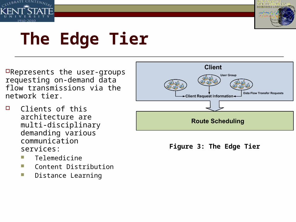
The Edge Tier
Clients of this architecture are multi-disciplinary demanding various communication services: Telemedicine Content Distribution Distance Learning
Figure 3: The Edge Tier
Represents the user-groups requesting on-demand data flow transmissions via the network tier.
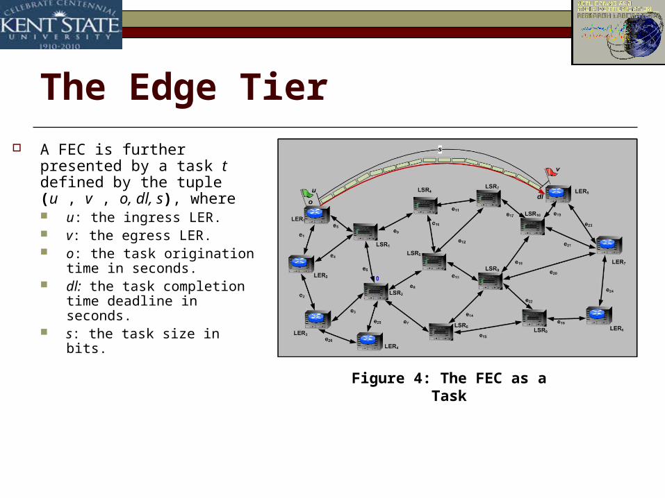
The Edge Tier
A FEC is further presented by a task t defined by the tuple (u , v , o, dl, s), where u: the ingress LER. v: the egress LER. o: the task origination time
in seconds. dl: the task completion
time deadline in seconds. s: the task size in bits.
Figure 4: The FEC as a Task

The Routing Tier
The main task of the route scheduling tier is computing time-scheduled routes in the underlying network domain.
Figure 5: The Routing Tier
Consists of the route scheduling solver.

The Routing Tier
Let set RT ={ r1, r2, …, ri,…, rn} defines a route schedule as a set of routes, where each task has a route (is committed to a task).
Figure 6: The LSP Specifications
Given a MPLS domain G = (N, E)
Let T denote the set of n tasks
Let the route (LSP) ri be a solution to task ti, defined as an ordered set of k node hops (switch routers)
Hi = {ui, ni,2,…, ni,j, …, ni,(k-1), vi}, or as k-1 link (edge) hops.
Li = {ei,1, ei,2,.., ei,j, …, ei,k-1}, where ei,j connects ni,(j-1) and ni,j.
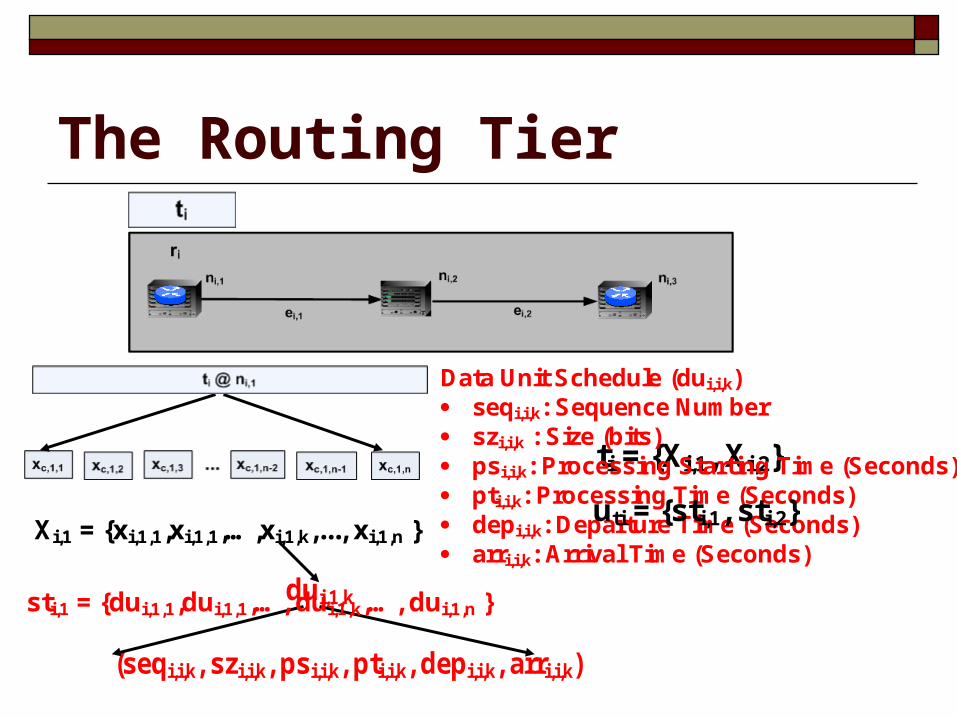
Xi,1 = {xi,1,1,xi,1,1,…,xi,1,k,..., xi,1,n }
The Routing Tier
ti = {Xi,1, Xi,2}
dui,1,k
(seqi,i,k, szi,i,k, psi,i,k, pti,i,k, depi,i,k, arri,i,k)
Data Unit Schedule (dui,i,k)· seqi,i,k: Sequence Number· szi,i,k : Size (bits)· psi,i,k: Processing Starting Time (Seconds)· pti,i,k: Processing Time (Seconds)· depi,i,k: Departure Time (Seconds)· arri,i,k: Arrival Time (Seconds)
sti,1 = {dui,1,1,dui,1,1,…, dui,1,k,…, dui,1,n }
uti = {sti,1, sti,2}

The Scheduling Tier
Figure 7: The Scheduling Tier
This tier consists of three entities: Node Resource Information Base (NRIB) Link Resource Information Base (LRIB) and Router server.

The Scheduling TierThe Node Resource Information Base (NRIB)
Node resources information includes: Available service capacity
(bps)
Total service capacity (bps)
Total input/output buffers capacity (bytes) and
Available input/output buffer capacities (bytes).
Figure 8: The NRIBxi,j,k
a
xi,j,k
b
Insert (out-rsvi,j,k)1
(k, i, ni,j, szi,j,k,(depi,j,k – pti,j,k), depi,j,k)
Insert (in-rsvi,j,k)2
(k, i, ni,j+1, szi,j,k, arri,j,k)
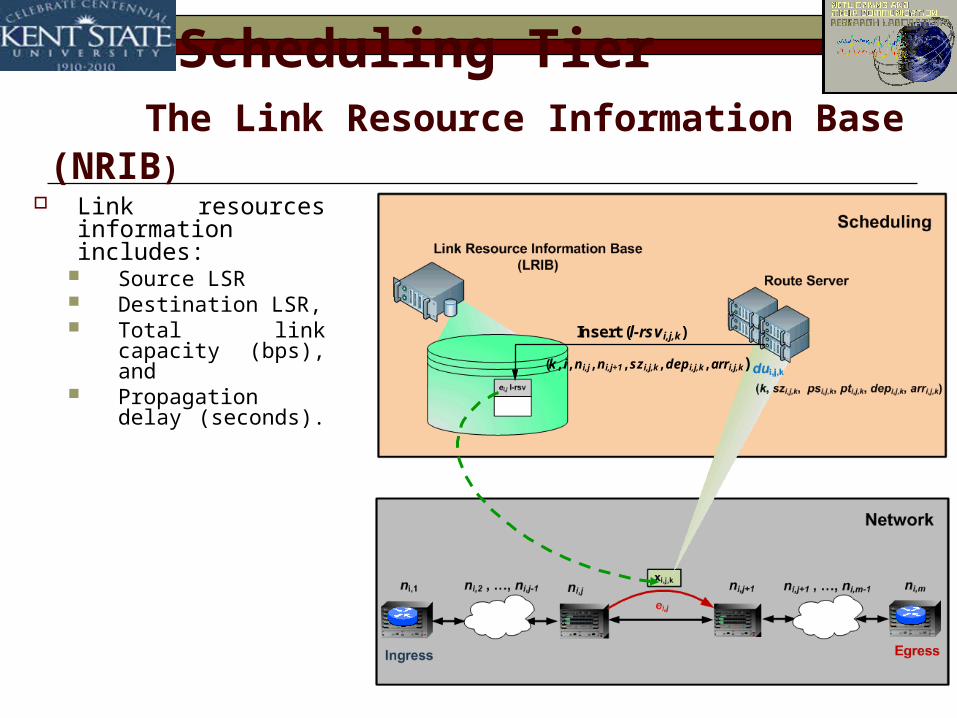
The Scheduling TierThe Link Resource Information Base (NRIB)
Link resources information includes: Source LSR Destination LSR, Total link capacity
(bps), and Propagation delay
(seconds).
Figure 9: The NRIB
Insert (l-rsvi,j,k)
(k, i, ni,j, ni,j+1, szi,j,k, depi,j,k, arri,j,k)
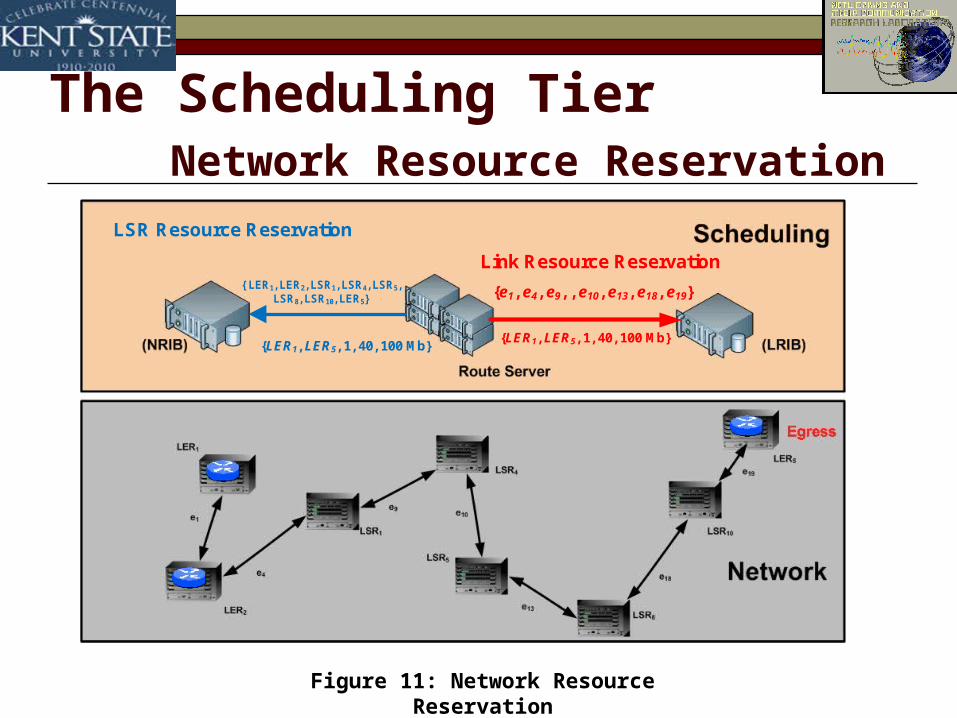
The Scheduling Tier Network Resource Reservation
Figure 11: Network Resource Reservation
{ LER1, LER2, LSR1, LSR4, LSR5, LSR8, LSR10, LER5}
LSR Resource Reservation
{LER1, LER5, 1, 40, 100 Mb}
Link Resource Reservation
{e1, e4, e9, , e10, e13, e18, e19}
{LER1, LER5, 1, 40, 100 Mb}
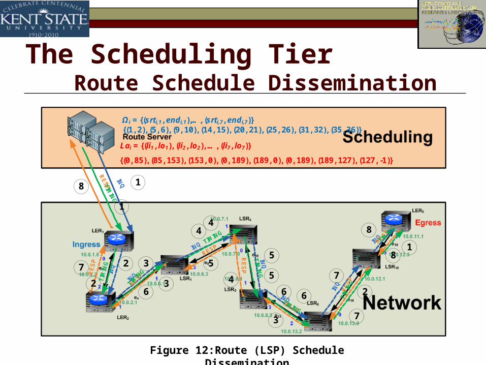
The Scheduling TierRoute Schedule Dissemination
INQ
INQ
INQ
INQ
INQ
INQ
INQ
INQ
1
2 3
4
5
6
7
8RESP
RE
SP
RESP
RE
SP
RESP
RESPRE
SP
RE
SP
1
2
3
4
5
6
7
8
Lai = {(li1, lo1), (li2, lo2), …, (li7, lo7)}
{(0, 85), (85, 153), (153, 0), (0, 189), (189, 0), (0, 189), (189, 127), (127, -1)}
TIMIN
G
1
2 3
4
5
6
7
8
TIM
ING
TIMIN
G
TIMINGT
IMIN
G
TIMING
TIM
ING
TIMIN
G
Ωi = {(srti,1, endi,1),…, (srti,7, endi,7)}{(1, 2), (5, 6), (9, 10), (14, 15), (20, 21), (25, 26), (31, 32), (35, 36)}
Figure 12:Route (LSP) Schedule Dissemination

Outline Introduction
The Scheduling-based Routing Network Architecture
Case Study: An Institutional Remote Data Backup & Recovery Network
Performance Evaluation.
Conclusion and Future Work

Case Study: An Institutional Remote Data Backup & Recovery Network
We utilize the Ohio Supercomputing Computing [6] network OSCnet as practical network backbone.
Safeguarding data and information against all types of disasters is an urgency.
Offline remote data backup & Recovery Networks serves an efficient solution.
In organizational Information centers, data & information backup is performed in a daily, weekly and monthly basis.

Case Study:The OSCnet Network Backbone
Figure 13: The OSCnet Network Backbone

Case Study:Backup Mirror Site Assignment
Table 1: Backup Mirror Sites Assignment

Case Study:Data Backup Transfer Demands
Table 2: Projected Daily Transfer Demands

Case Study:Critical Performance Challenges
Figure 14: Sample Average Shortest Path Length
Stable
Chaotic Will Chock out other bandwidth
contending Applications

Case Study:Critical Performance Challenges
Figure 15: Sample Aggregate Shortest Path Load

Figure 16: The Four-Tier OSCnet-based Network Architecture
Case Study: The Network Architecture

Outline Introduction
The Scheduling-based Routing Network Architecture
Case Study: An Institutional Remote Data Backup & Recovery Network
Performance Evaluation.
Conclusion and Future Work
Performance Evaluation
To demonstrate the performance incentives of scheduled-based data transfer over the classical transfer scheme.
Compares the performance achieved by scheduled backup data transfer to the classical unscheduled scheme.
This study is conducted as a simulation study of the OSCnet network backbone shown by Figure 13.

Simulation Experiment-1 Setup
Link capacity allocation:
Unscheduled: Day = 100%, Night = 100% Scheduled: Day = 10%, Night = 90%
Number of Tasks: 156.
Performance Metrics: Average Shortest Path Length at Link Load 90% Aggregate Shortest Path Load at Link Load 90%
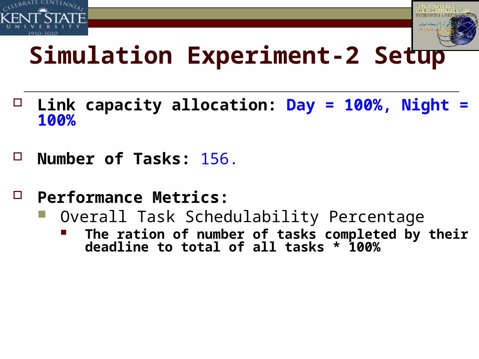
Simulation Experiment-2 Setup
Link capacity allocation: Day = 100%, Night = 100%
Number of Tasks: 156.
Performance Metrics: Overall Task Schedulability Percentage
The ration of number of tasks completed by their deadline to total of all tasks * 100%

Simulation Experiment-1 Results
Figure 16: Average Shortest Path Length
Unscheduled
Scheduled
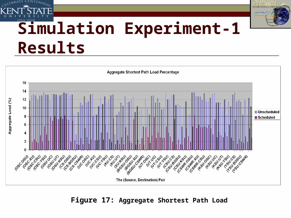
Simulation Experiment-1 Results
Figure 17: Aggregate Shortest Path Load

Simulation Experiment-2 Results
Figure 17: Overall Task Schedulability
Outline Introduction
The Scheduling-based Routing Network Architecture
Case Study: An Institutional Remote Data Backup & Recovery Network
Performance Evaluation.
Conclusion and Future Work

Conclusion and Future Work
On the basis of the performance evaluation stud, it can be concluded that Scheduling-based routing significantly improves: The Average Shortest Path Length. The Aggregate Load of the Shortest Path. The Overall Task Schedulability.
Presented a four-tier scheduling-based routing architecture namely DCN@MPLS.
Demonstrated a OSCnet-based remote data backup case study.

Conclusion and Future Work
The Scheduling-based data backup and recovery Near-optimal mirror site exploration and Selection Heuristics.
Hierarchical scheduling-based routing network architecture DCN@MPLS is a centralized architecture.
MPLS & CR-LDP Protocol Extensions Timed Route Schedule Dissemination in MPLS networks
Pathway Intermittency Route Scheduling in Physically/Logically Intermittent Networks

Thank You !

References
[1] The Internet2, Wikipedia, url: http://en.wikipedia.org/wiki/Internet2.
[2] Internet2 Consortium, “Internet2’s Dynamic Circuit Network”, 2008.
[3] E. Rosen, A. Viswanathan, and R. Callon, “Multiprotocol Label Switching Architecture”, RFC 3031, January, 2001.
[4] O. Tahboub, “DCN@MPLS: A Network Architectural Model for Dynamic Circuit Networking at Multiple Protocol Label Switching”, TR-2009-02-01, MediaNet Lab, , 2009.
[5] Tahboub, O., Khan, J., “DCN@MPLS: A Network Architectural Model for Dynamic Circuit Networking at Multiple Protocol Label Switching”, The First International Workshop on Concurrent Communication ConCom 2009, Seattle, WA, 2009.
[6] The Ohio Super Computing Network, url: http://www.osc.edu/oscnet/