i |

A SCALABLE RECOMMENDER SYSTEM

Using Latent Topics and Alternating Least Squares

Techniques

András Péter Kolbert

Dissertation presented as partial requirement for obtaining

the Master’s degree in Advanced Analytics

i |

A SCALABLE RECOMMENDER SYSTEM

Using Latent Topics and Alternating Least Squares Techniques

20

17

András Péter Kolbert

MAA

MAA

i |

NOVA Information Management School

Instituto Superior de Estatística e Gestão de Informação

Universidade Nova de Lisboa

A Scalable Recommender System Using Latent Topics and Alternating

Least Squares Techniques

by

András Péter Kolbert

Dissertation presented as partial requirement for obtaining the Master’s degree in Advanced

Analytics

Advisor: Mauro Castelli

August 2017

i |

Abstract

A recommender system is one of the major techniques that handles information overload

problem of Information Retrieval. Improves access and proactively recommends relevant

information to each user, based on preferences and objectives. During the implementation

and planning phases, designers have to cope with several issues and challenges that need

proper attention. This thesis aims to show the issues and challenges in developing high-quality

recommender systems.

A paper solves a current research problem in the field of job recommendations using a

distributed algorithmic framework built on top of Spark for parallel computation which allows

the algorithm to scale linearly with the growing number of users.

The final solution consists of two different recommenders which could be utilised for different

purposes. The first method is mainly driven by latent topics among users, meanwhile the

second technique utilises a latent factor algorithm that directly addresses the preference-

confidence paradigm.

Keywords: job recommendation, matrix factorisation, alternating least squares, latent dirichlet allocation, scalable

ii |

Acknowledgements

First, I would like to thank my thesis instructor, Mauro Castelli, for the guidance and support

he has provided me throughout the whole process, from the very beginning to the end. I have

been extremely lucky to have a supervisor who cared so much about my work and who

responded to my questions and queries promptly.

Secondly, I must express my gratitude to Ildikó Kolbert, my sister, for her continued support

and suggestions. I was amazed by her willingness to proof read countless pages.

Furthermore, I would like to thank to Steve Austen, for the suggestions he made in reference

to this work.

Completing this work would have been all more difficult without a flatmate and friend like

Matt Parkin, who experienced all of the ups and downs of my research and helped me out

whenever I needed.

Finally, I would like to acknowledge university colleagues and friends who supported me

during my time in Lisbon. I feel honoured to have had the chance to work together with Beáta

Babiaková, Carolina Duarte and Illya Olegovich Bakurov on various data science projects and

continuously learn from them. Also, I would like to thank Andrea Vergati, Federico Sisci and

Giuseppe Parisi for the happy time we spent together during my time in Lisbon.

iii |

Table of Contents

1 Chapter 1 ....................................................................................................................... 1

1.1 Introduction ............................................................................................................. 1

1.1.1 Context ............................................................................................................ 1

1.2 Motivations ............................................................................................................. 2

1.2.1 Benefits for the providers ................................................................................. 2

1.2.2 Benefits for the users ....................................................................................... 2

1.3 Document Structure ................................................................................................ 3

2 Chapter 2 ....................................................................................................................... 4

2.1 Recommender Systems overview ........................................................................... 4

2.2 Formal definition ..................................................................................................... 5

2.3 User preferences .................................................................................................... 6

2.3.1 Implicit and explicit feedback ........................................................................... 6

2.4 Bias in user preferences ......................................................................................... 7

2.5 Related works ......................................................................................................... 7

3 Chapter 3 ....................................................................................................................... 9

3.1 Basic algorithms ..................................................................................................... 9

3.2 Heuristic recommenders ....................................................................................... 10

3.2.1 Similarity measures........................................................................................ 10

3.3 Content-based recommenders .............................................................................. 12

3.3.1 Pre-processing ............................................................................................... 13

3.4 Collaborative filtering ............................................................................................ 15

4 Chapter 4 ..................................................................................................................... 17

4.1 Matrix Factorisation ............................................................................................... 17

4.2 Principal Component Analysis .............................................................................. 19

4.3 Singular Value Decomposition .............................................................................. 20

4.4 Limitations of most optimization algorithms ........................................................... 23

4.5 Additional challenges and solutions ...................................................................... 24

4.5.1 Biases ............................................................................................................ 24

4.5.2 Temporal dynamics........................................................................................ 24

4.5.3 Synonymity .................................................................................................... 25

5 Chapter 5 ..................................................................................................................... 27

5.1 Hybrid recommenders ........................................................................................... 27

5.1.1 Parallelized hybridization ............................................................................... 27

iv |

5.1.2 Pipelined approach ........................................................................................ 30

5.1.3 Monolithic design ........................................................................................... 32

5.1.4 Hybrid System Experiments ........................................................................... 33

6 Chapter 6 ..................................................................................................................... 35

6.1 Challenges ............................................................................................................ 35

6.1.1 Cold start ....................................................................................................... 35

6.1.2 Sparsity .......................................................................................................... 35

6.1.3 Diversity and serendipity ................................................................................ 37

6.1.4 Scalability ...................................................................................................... 38

7 Chapter 7 ..................................................................................................................... 39

7.1 Evaluating recommender systems ........................................................................ 39

7.1.1 Measures ....................................................................................................... 40

7.1.2 Methodology .................................................................................................. 41

8 Chapter 8 ..................................................................................................................... 42

8.1 Problem formulation .............................................................................................. 42

8.2 Used technology ................................................................................................... 43

8.3 Description of data ................................................................................................ 44

8.4 Data preparation and exploration .......................................................................... 45

8.5 Challenges ............................................................................................................ 50

8.5.1 Cold-start problem ......................................................................................... 50

8.5.2 Scalability ...................................................................................................... 51

8.5.3 Sparsity .......................................................................................................... 51

8.6 Model training ....................................................................................................... 51

8.6.1 Latent user profile segments .......................................................................... 52

8.6.2 Alternating least squares ............................................................................... 53

8.6.3 Recommending to existing and online updating for new users ....................... 54

8.7 Evaluation methods .............................................................................................. 55

8.8 Optimisation and training ...................................................................................... 56

8.8.1 Latent topic approach .................................................................................... 56

8.8.2 Alternating least squares ............................................................................... 57

8.8.3 Overall optimisation results ............................................................................ 62

9 Chapter 9 ..................................................................................................................... 63

9.1 Conclusions .......................................................................................................... 63

9.2 Future work ........................................................................................................... 64

10 Chapter 10 ............................................................................................................... 65

10.1 References / Bibliography ..................................................................................... 65

v |

Table of Figures

Figure 1 - A traditional utility matrix example representing movie ratings on a 1–5 scale .................... 5

Figure 2 - Collaborative Filtering at Spotify (Bernhardsson, 2013) ....................................................... 18

Figure 3 – Parallelized hybridization (Brusilovsky et al, 2007) .............................................................. 27

Figure 4 – Weighted scheme (Brusilovsky et al, 2007) ......................................................................... 28

Figure 5 – Switching technique (Brusilovsky et al, 2007)...................................................................... 29

Figure 6 – Mixed strategies (Brusilovsky et al, 2007) ........................................................................... 29

Figure 7 – Pipelined approach (Brusilovsky et al, 2007) ....................................................................... 30

Figure 8 – Cascade hybrids (Brusilovsky et al, 2007) ............................................................................ 30

Figure 9 – Meta-level hybrids (Brusilovsky et al, 2007) ........................................................................ 31

Figure 10 – Monolithic hybrids (Brusilovsky et al, 2007) ...................................................................... 32

Figure 11 – Feature combination hybrids (Brusilovsky et al, 2007) ...................................................... 32

Figure 12 – Feature augmentation hybrids (Brusilovsky et al, 2007) ................................................... 33

Figure 13 – Users registered location ................................................................................................... 47

Figure 14 – Job postings registered position ........................................................................................ 48

Figure 15 – Number of interactions since jobs were posted ................................................................ 48

Figure 16 – Average number of interactions ........................................................................................ 49

Figure 17 – Account’s event interactions ............................................................................................. 50

Figure 18 – LDA technique to derive recommendations ...................................................................... 53

Figure 19 – ALS pseudo code ................................................................................................................ 54

Figure 20 – Rank Score by latent topics ................................................................................................ 57

Figure 21 – Rank score by regularisation parameter ............................................................................ 58

Figure 22 – Rank score by iterations ..................................................................................................... 59

Figure 23 – Computational costs by iterations ..................................................................................... 59

Figure 24 – Rank score by alpha values ................................................................................................ 60

Figure 25 – Computational costs by latent features ............................................................................. 61

Table of Tables

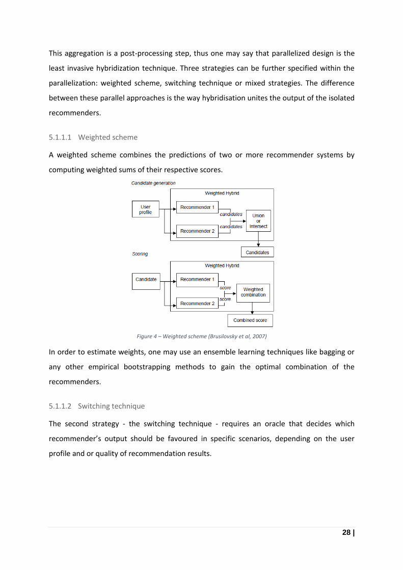
Table 1 – Evaluation metrics (Avazpour et al, 2014) ............................................................................ 40

Table 2 – Descriptive Statistics.............................................................................................................. 45

Table 3 - Result summary for 3-fold cross validation ........................................................................... 61

1 |

1 Chapter 1

1.1 Introduction

1.1.1 Context

The volume of structured and unstructured data has grown at an exponential scale in recent

years. As a result of this rapid data growth, we are deluged with information and a plethora

of choices in any product or service. It is natural to get lost in the range of options. Information

overload has reached a point where the available information cannot be processed simply by

the human mind, it needs special guidance.

Recommender systems (hereinafter RS) are one of the major techniques to handle this

information overload problem from the field of Information Retrieval. These systems have

emerged to help users navigate through this increased content, often leveraging user-specific

data that is collected from users. It improves access and proactively recommends relevant

information to each user based on preferences and objectives.

During the implementation and planning phases, designers have to cope with several issues

and challenges that need proper attention. This thesis aims to show the issues and challenges

in developing high-quality recommender systems. This paper also aims to solve a current

research problem in the field of job recommendations. More specifically, with a given large

dataset that consists of anonymized user profiles, job postings, and interactions, the aim is to

predict the job postings that a user will positively interact with by clicking on, or bookmarking

it. This prediction is will be evaluated on various approaches while using a scalable

computation solution.

The project makes use of Apache Spark, a distributed big data processing framework. The

study will introduce an algorithmic framework built on top of Spark for parallel computation

which allows the algorithm to scale linearly with the growing number of users. The use of

Spark also provides the advantage of interactive computation and minimal processing time as

compared to traditional MapReduce paradigm. This implementation enable us to process

more than 230 million interactions from 1.5 million users in 5 months timeframe.

2 |

1.2 Motivations

The following section assess the possible benefits and motivations for both users and

providers for developing recommender systems.

1.2.1 Benefits for the providers

One out of the many opportunities for the providers, is to get a better understanding of users’

needs. Describing and knowing users’ preferences can boost sales figures, marketing activity,

product performance or even their supply chain management by improving production or

logistic efficiency. For instance the logistic efficiency increase can be achieved by investigating

various item associations, based on geographical area which allows the businesses to monitor

and balance stock levels in an optimal manner. Having known the item associations and

having optimised stock level, the users are targeted with relevant recommendations, at the

right time and place. This relevancy leads to an enhanced user experience which implies

higher retention rate to the business owners. Furthermore, it also enables the providers to

efficiently solve the so called long-tail problem. The long-tail refers to items that are rare and

obscure. Online vendors, unlike retailers can have these items on “stock”, using a broad

meaning for stock because frequently there’s no physical entity to store at all. A

recommender system can ensure that having a more diverse online platform, we can still

communicate to the right people and target relevant segments with matching products. One

positive side of optimising customer journeys is to generate more sales, but also to satisfy

users’ needs to a greater extent.

1.2.2 Benefits for the users

Recommender systems (RS) are not only beneficial for the service providers but also to the

users (PU et al, 2011). RS can help providers identify latent needs, desires or preferences

which a consumer might not be able to realise by himself/herself, due to the lack of

information about the product's availability.

For instance, finding an interesting and informative article that one may not look for

specifically, but may take pleasure in reading after being recommended. Users may also find

their most desired job posting due to a recommendation which might have a long term impact

on their life.

3 |

To conclude, one may see that this level of personalisation can be used in varying

circumstances for various benefits but it is worth emphasizing that in most cases it is a win-

win scenario for both parties.

1.3 Document Structure

This paper is structured in nine chapters.

Chapter 2 presents an overview about recommender systems. It includes a general

introduction, a formal definition and the relevance of such systems. It also shows in more

details the two different methods of rating data and describes the major difference in

modelling them. The chapter closes with detailing the most relevant related works and

research platforms.

Chapter 3 describes basic and heuristic based recommenders, highlighting their strengths and

weaknesses.

Chapter 4 presents additional advanced and model based techniques that the current state

of the art generally favours for specific problem formulations.

Chapter 5 gives a detailed overview about hybridization and presents the different strategies

in depth.

Chapter 6 presents the main challenges that need special attention during the practical

implementation phase.

Chapter 7 describes the main metrics and methodologies used for evaluating solutions in the

field.

Chapter 8 presents a job recommendation problem and propose a scalable solution. Here it

is further explained how the algorithmic approach works and also the used technology for

implementation phase, experimental setup and result analysis to understand the current

benefits and drawbacks of this solution. Finally, a short summary and discussion is presented

about the results.

Chapter 9 presents some conclusions about the presented work and a discussion about future

research lines.

4 |

2 Chapter 2

This chapter presents an overview about recommender systems, which is followed by a

formal definition. It is followed by a description of the different user feedbacks, related works

and the chapter end with categorising the currently active research hubs.

2.1 Recommender Systems overview

The concept of Recommender Systems (RS) initiates from the idea of information reuse, and

persistent preferences. RS can be defined as the set of software tools and techniques, that

provide suggestions for items that are of interest for a given user profile. (Ricci et al, 2011)

RS has the ability to guide users in a personalized way towards interesting objects in a large

search space (Burke, 2002). A naive user may not even recognise that most of their online

activities are supported and influenced by various recommendations in order to provide them

relevant content which can help in their decision making process. This guidance is the

system’s ability to predict whether an individual would prefer an item based on their profile.

The overall aim of such systems is to deal with the information overload problem by retrieving

vital information out of a large search space.

The structure of such systems depends on the particular domain and on the characteristics of

the available data. The most popular domains include social tags, search queries, social

connections, books, news, movies, music, services and products in general. There are also

recommender systems for experts, collaborators, jokes (Eigentaste, 2001), restaurants (Ricci

and Nguyen, 2017), garments (Iwata et al, 2017), financial services, life insurance, online

dating, Twitter pages (Gupta et al, 2013), and many others.

The large number of domains using RS is a testimony to the several usefulness of this

technique in enhancing provider-user interactions.

5 |

2.2 Formal definition

A traditional recommender system problem consists of a set of users, items and ratings. Let’s

introduce the following notation:

● Users: u = {u1, u2, . . . , un} U ∈ U1×n

● Items: I = {i1, i2, . . . , im} I ∈ I1×m

● Ratings: R = {r11, r12, . . . , rnm} R ∈ Rn×m

rui element is devoted to the rating, interaction or any sort of feature which represents a user

u ∈ U interest on a particular item i ∈ I. Generally, recommender problems have to tackle a

very sparse rating matrix, suggesting that there are many unknown relations between an item

and a user u.

Figure 1 - A traditional utility matrix example representing movie ratings on a 1–5 scale

One may note that most of the user-movie pairs are blanks, which means that the user has

not rated the movie yet. In this example the users have rated 36% of the items (9/25) has

higher density than most real word scenarios. This means that a typical user may rate or

interact with only a tiny fraction of all available items. According to the literature, the density

of the rating matrix in commercial recommender systems is often less than 1% (Tang et al,

2013, p.4).

The usual aim of any recommender systems is to be able predict the missing ratings for the

user ui on a non-rated item ij; or to recommend particular item sets or neighbourhoods which

are the most likely to be of interest for the given users.

6 |

2.3 User preferences

2.3.1 Implicit and explicit feedback

Fundamentally, the utility matrix shown previously can contain two types of rating data,

which need to be distinguished and modelled differently. Most convenient is the high quality

explicit feedback, which includes explicit input from users regarding their interest in products,

typically using a concrete rating scale. This type of feedback can be directly interpreted as the

user’s preferences, making it easier to make extrapolations from the data to predict future

ratings. For instance, Netflix collects star ratings for movies or YouTube users indicate their

preferences for videos by hitting thumbs-up and down buttons. Although explicit feedback

tends to have higher quality, and is in general easier to model, this kind of pure information

is not always available.

Thus, one may use behavioural data to infer user preferences from the more abundant

implicit feedback, which indirectly reflect opinion through observing user behaviour: such as

purchase history, browsing history, search patterns or mouse movements. The aim is to

transform user behaviour into user preferences which can be a difficult task to solve.

Modelling implicit feedback is a difficult but an important problem.

Essentially, there are two main challenges in modelling preferences using implicit feedback

data. By observing users behaviour, we can infer which items they probably like and thus

chose to consume. However, this does not necessarily indicate a positive view of the product.

For instance observing a purchase for an individual, may have just happened for gifting

purposes on behalf of someone else, or took place but the user was not satisfied with the

item and eventually it leads to a negative experience. Implicit feedback is not capable of

accounting for these factors on its own.

Meanwhile, explicit recommenders tend to focus on the gathered information – those user-

item pairs that we know their ratings – which provide a balanced picture on the user

preference. Thus, the remaining user-item relationships, which typically constitute the vast

majority of the data, are treated as “missing data” and are omitted from the analysis. This is

impossible with implicit feedback, as concentrating only on the gathered feedback will leave

us with the positive feedback, greatly misrepresenting the full user profile. Hence, it is crucial

to address also the missing data, which is where most negative feedback is expected to be

7 |

found. In implicit feedback datasets, non-interaction of a user with an item does not

necessarily indicate that an item is irrelevant for the user, it can also mean that the user is

unaware of the item’s existence. The significance of positive feedbacks are much larger than

the missing negative feedbacks, therefore the feedback types should be weighted

(normalized) differently in the model.

2.4 Bias in user preferences

Another important aspect of user feedback is the user bias. Raw ratings also encapsulate the

user’s viewpoint, the way they rate items. There are always some users who tend to give

higher (or lower) ratings than others (explicit), or on average be more active in general than

the others (implicit), or some items may be higher (or lower) rated than others, because they

are widely perceived as better (or worse) than the others. For instance, two users liking and

disliking similar movies, but one being a bit more critical and rates average movies 1.5-2 out

of 5 meanwhile the other user is a movie enthusiast who rates the average films 4 out of 5.

According to previously conducted experiments, most recommender systems perform better

if user and item biases are taken into account (Adomavicius et al, 2014). Therefore a proposed

solution is explained in a later section.

2.5 Related works

Recommender Systems is a burgeoning research area. There are multiple mediums that foster

the advancement of this field:

● Research articles, conferences and workshops

○ ACM Conference on Recommender Systems - The most significant annual

conference where all the papers focus on recommender technology and

applications.

○ ACM Transactions on Information Systems

○ ACM UMAP (User Modeling, Adaptation and Personalization) User Modeling.

○ ACM HT (Hypertext and Social Media) - Hypertext and Social Media (HT)

WWW, ACM SIGIR - many relevant discussions related to RSs.

○ ACM IUI FLAIRS, Web Intelligence

● Undergraduate and graduate level online/offline courses, blog posts and tutorials.

8 |

● Recommender System handbook (Ricci et al, 2011), and several academic journals

related to RSs were published. A few examples AI Communications (2008), IEEE

intelligent Systems ACM Transactions on Computer-Human Interaction (2005) and

many others.

● Netflix prize competition - One of the key events that significantly boosted research in

RSs.

Other relevant research papers will be presented throughout the paper.

9 |

3 Chapter 3

The following chapter presents various algorithms; starting from basic type of algorithms to

more complex forms.

3.1 Basic algorithms

The simplest type of recommendations are given by non-personalised (NP) systems. As one

may suspect, these methods do not take into account an individual’s preferences thus the

recommendations are identical for all the users. These can be seen as an item suggestion or

an item set that the user might like although it is independent of the specific consumer

behaviour (Poriya et al, 2014; Khatwani and Chandak, 2016). NP systems use data about what

consumers have said about an item and derive a global expectation of how an average user

would rate them. NP can be mainly categorized into two types: aggregated opinion

recommender and basic product association recommender. Various examples exist for the

NP approach, as it is often combined with personalised recommenders in the initial phase

when there is no available information about the given user.

For instance, restaurant guides like TripAdvisor or Yelp tend to use aggregated opinion

techniques to display ratings of items. News websites also make use of this type of algorithm

by showing the most popular articles or trending news to the users. Many commercial

websites also show the products with the highest demand on their page as a form of

recommendation. Aggregated opinion techniques can be useful to obtain a view of what the

vast majority of people prefer, however, a major disadvantage is they lack context around the

suggestion.

An example can be given using the previously mentioned most popular articles. In general,

the value of information tends to decrease over time (Moody and Walsh, 1999). Using the top

average ratings from users (explicit) or most visited (implicit) pages, may suggest articles that

many users were interested in an article from 10 years back, following a live feed about an

ongoing election. Most probably this article became less and less relevant over time, even if

it is classified as the most popular page. This example illustrates one of the drawbacks of using

only top rated items for recommendation as it misses the time as contextual information but

that is easy to avoid with recency based trending. In addition to the lack of context, these

10 |

measures are able to describe a group of observations but fail to recognise an individual’s

taste and adjust suggestions accordingly.

The NP systems can be a good approach when the system lacks any sort of interactions

(cookies, registered users, location etc.) so cannot associate behaviour data to a specific user.

In these anonym cases, blindly showing items which tend to be the most favoured on average

can be a solution. However, these assumptions may not be relevant for many users.

3.2 Heuristic recommenders

After reviewing the most basic aggregated approaches, the following section is intended to

describe heuristic based approaches.

Heuristic (also called memory-based) RS employ specific heuristic formulae - such as vector-

based similarity or correlation measures - to calculate recommendations. For memory based

recommenders, the prediction process needs similarity evaluation in order to generate

nearest neighbourhoods which can be utilised for score prediction. Memory-based

techniques continuously analyse user and item data to calculate recommendations and can

be classified in the following main groups: Collaborative Filtering, Content-Based (CB)

techniques and Hybrid approaches.

3.2.1 Similarity measures

Modelling distance and similarity between various features is an important step in

recommender systems. Chiefly, the aim is to find similar items and users in order to find a

relevant neighbourhoods. This section shows some of the popular similarity measures that

are widely used in collaborative filtering.

Probably the simplest distance measures out of the many is Euclidean distance (Gower, 1982)

and its generalised counterpart, the Minkowski distance (Schafer, 2007).

Euclidean distance:

● N number of dimensions

● and are the attributes of data objects x and y

Minkowski distance (generalization of Euclidean distance):

11 |

Another common approach is cosine similarity (Sidorov, 2014). As the name suggests, this

measures the similarity based on the cosine of the angle between vector x and y in an n-

dimensional space.

Similarity can also be assessed based on correlation which means the linear relationship

between objects. The most commonly used correlation in recommender systems (Ricci et al,

2011) is Pearson correlation, which can be formulated as follows:

● are the standard deviation of the corresponding vectors

Pearson’s correlation coefficient ranges from negative one to positive one. Positive

relationship indicates that the variables increase or decrease together, whereas negative

value implies that the variables move in the opposite direction to each other. Traditionally,

most of the recommender systems have used either the cosine similarity or the Pearson

correlation - or one of their many variations.

For instance Adjusted Cosine (AC) whereas mean-centred ratings are compared. This mean-

centred property eliminates one of the important drawbacks of similarity computation using

cosine measure: the difference in rating scale between different users are not taken into

account. The adjusted cosine similarity offsets this drawback by subtracting the

corresponding user average from each co-rated pair. (Wei et al, 2012)

12 |

Formally, the similarity between items i and j using this scheme is given by:

● average rating of user u

● adjusted rating scale

Broadly speaking, the described similarity scores allow the model to select trusted neighbours

whose ratings are used in the predictions and they also provide the means to give more, or

less importance to these neighbours in the prediction. Therefore, the computation of the

similarity weights is a crucial part of building neighbourhoods based recommender systems,

as it can have a significant impact on both its accuracy and performance.

The previously mentioned neighbourhood can be defined by items (content based

recommenders) or users (collaborative filtering). Collaborative and content-based

recommender algorithms are the most applied and most popular approaches among

RS (Lü et al, 2012; Ricci et al, 2011). The following two sections provide an overview of

these methods.

3.3 Content-based recommenders

Content-based recommenders (CB) make use of content characteristics of items that the user

has previously rated or favoured. The basis of these systems is to analyse a set of documents,

descriptions or any other attributes of items and build a profile of user interests based on

these features. This profile is a structured representation of user interest for the purpose of

recommending new relevant items.

One may note that, the users are independent in CB approach, as these techniques exploits

solely ratings provided by the user to build his/her own profile. It means that these systems

can tackle the so-called new-items problem, which is one specific type of cold-start problem.

They are capable of making recommendations on items, which are not yet rated by any users.

Although CB methods resolve the new item problem, they still suffer when a new user

appears in the system (Ricci et al, 2011). In case a new user registers, these systems

13 |

fail to make recommendations, hence the user profile is missing. This topic can be

tackled in various ways which are presented in chapter six.

It is worth pointing out that CB can provide explanation to the users; the descriptions that

caused an item to be recommended. Explanation on CB systems can be provided by explicitly

listing content features that can promote users’ trust in the system. Transparency is an

important aspect of an RS.

Conversely, CB recommenders are prone to become over specialised and lack the capability

to find the unexpected. The system recommends items whose score are high when matched

against the user profile, therefore the user gets similar items as recommendations. This leads

to another well-known issue in RS which is the serendipity problem. Serendipity can be

described as a surprise, delight in a sense that something unexpected resulted, this problem

is explained in more depth in chapter six.

3.3.1 Pre-processing

In order to perform CB recommendations, various pre-processing steps are required to

structure and extract features from the available information about the items. Most of the

techniques which are applied through the content analysis stage are taken from Information

Retrieval Systems.

In some cases features can be immediately available for use in modelling similarity based on

the content. The most obvious example is user ratings (as it was shown before). In addition,

item features can also be used for positioning and linking items together. An example is the

product category for an item in an e-commerce website.

In some cases these features are not that obvious. Feature engineering is needed to transform

and discover the information from the given dataset. The data can be in various format

document collection or corpus like news articles, blog posts, web pages, research papers, item

descriptions or visual content like images or videos. For the textual data, the overall aim is to

be able to identify a set of words or characteristics which can separate the dissimilar items

and cohere the similar ones.

Term Frequency (TF) and Inverse Document Frequency (IDF) is used to model these additional

features. These concepts are mainly used in information retrieval systems but can also be

14 |

applied in content based filtering mechanisms. They are used to determine the relative

importance of a document, article, news item, movie, book or any sort of textual corpus.

(Jurafsky and Martin, 2000)

The frequency of a word in a document can be formulated as follows:

,

Where

● is the number of times word i appears in document j

● is the number of most frequent term in the document j

TF measures how relative frequency of a specific term in document j. It is not simply the actual

frequency, since documents can have varying length, thus it is need to be normalised. For this

purpose, the frequency is often divided either by the length of the documents, or by the

frequency number of the most occurring term in the document (as in the above formula) to

prevent a bias towards longer documents.

IDF is the inverse of the document frequency among the whole corpus of documents.

Where

● N is the Total number of documents

● Ni is the number of documents with term t in it

IDF measures how much information the word provides and it negates the effect of high

frequency words in determining the importance of an item. The sum product of TF and IDF

gives the TF-IDF score which values describe a vector space. This value space can be used to

find similar items by a distance measure which can help quantify the interrelationship

between items and eventually create new useful features.

15 |

3.4 Collaborative filtering

Whereas content based systems try to recommend similar items to those items that a given

user has previously liked, collaborative RS tries to identify a group of users who share similar

characteristics or tastes. CF relies on pattern of users’ behaviour or ratings without the need

for exogenous information about either items or users. It tries to capture the interactions

between users and items by computing a similarity index between users and recommend

items.

Commonly used CF methods are correlation based (Manolis and Konstantinos, 2004, also see

Mahapatra et al, 2011), Bayesian network (Miyahara and Pazzani, 2000) and association rules

techniques (Lin et al, 2002).

Generally, users are clustered based on their preferences with the aim of representing group

of individuals who tend to share common taste and like similar items. The cluster that has

the highest correlation with the specific target user can be used in collaborative

recommender systems to represent affinities among user’s preferences.

The neighbourhood based approach uses the ratings to find the most correlated features in

order to predict ratings for new items. These algorithms require computation that grows with

both the number of customers and the number of products. With millions of customers and

products, a typical web based recommender system running existing algorithms will suffer

serious scalability problems. The majority of implementations are not scalable therefore can

be questionable for most real-world scenarios (Sarwar et al, 2002).

Contrastingly, model based approaches use ratings to create a predictive model. These

models are based on an offline pre-processing or "model-learning" phase at run-time. In this

phase, user and item features are captured by a set of model parameters which are learned

from the training set and used to predict ratings.

Therefore, the recommendations are produced using the learned model which makes it

possible to apply to real-world problems. However, these models are usually updated or re-

trained periodically.

Several different model based techniques have been applied in terms of RSs, including

Bayesian belief nets CF (Miyahara and Pazzani, 2000), Artificial neural network (ANN) (Oord

et al, 2013; Kim et al, 2005), Markov Decision processes based Collaborative Filtering

(Brafman et al, 2012), Latent Semantic Analysis (Di Noia, 2012), Latent Dirichlet Allocation

16 |

(Agarwal and Chen, 2010), Boltzmann Machines (Abdollahi, 2016), Support Vector Machines

(SVM) (Min and Han, 2005) and Singular Value Decomposition (SVD) (Koren et al, 2009). The

following chapter provide details about model based recommenders.

17 |

4 Chapter 4

In machine learning, the goal is to find solutions to problems which are generalizable and can

be applied on unseen data with certain confidence. In order to obtain a statistically sound and

reliable result, the amount of underlying data needs to support this result while considering

that the computation complexity often grows exponentially with the dimensionality.

In the context of RS, the number of items available in a dataset is usually much higher than

the number of items rated by a user. This sparsity is a widely-known problem in the

recommender systems literature (Amatriain, 2011). The dataset defines a sparse high-

dimensional space which means that the number of observations by features is not

significantly numerous. This phenomenon is usually referred as the curse of dimensionality.

The following sections will describe the main data pre-processing dimensionality reduction

techniques - Principal Component Analysis, Singular Value Decomposition and a few

enhancements - which can tackle this serious problem. In addition to providing information

about different matrix factorisation techniques, this chapter also shows how to efficiently

transform these approaches into a supervised model based dimensionality reduction

technique and a powerful recommender system.

4.1 Matrix Factorisation

On top of reducing the dimensionality, matrix factorisation methods can also help uncover

latent features that explain observed ratings. Furthermore, the identified factors might be

used to explain interrelationships among the variables too. The latent factors are capable of

solving the synonym problem, which refers to the tendency of a number of the same or

very similar items to have different names or entries. The prevalence of synonyms

increase the competitive advantage of the model based matrix factorisation

approaches over the memory based CF systems. The synonyms problem is detailed in

more depth after introducing the different matrix factorisation techniques.

The latent factor approach tries to explain ratings by characterising both items and users set.

For instance a song recommender system’s item factors might measure obvious dimensions,

such as rock versus pop, amount of bass or acousticness factors.

18 |

These factors could be easily digested for humans though this is not the case for most of the

real world applications.

Figure 2 - Collaborative Filtering at Spotify (Bernhardsson, 2013) The example above illustrates that latent factors might correspond with human assumptions

like music genre. As the graph shows, the two latent factors separate classical music well from

the others, however the other genres are not clearly separated.

In addition to describing items, these factors can also be applied for users. In this case, each

factor measures how much the user like the item that score high on the corresponding factor.

It captures the user’s overall interest in the item’s characteristics.

Matrix factorisation models map both users and items to a joint fact space, whereas user-

item interactions are modelled as inner products in that space. The resulting dot product is

captures the previously mentioned interrelationships between users and items. This

approximates the rating matrix leading to the following estimates:

Where

● pu indicates how much user likes f latent factors

● qi measures how much one particular item obtains from f latent factors

The dot product of the two gives the approximation on the u user’s taste on i item. Matrix

factorisation is known as one of the most successful realizations of latent factor models and

can produce better accuracy than classic nearest neighbour methods when dealing with

19 |

product recommendations because of the incorporation of additional information such as

implicit feedback and temporal effects (Guan et al, 2016).

4.2 Principal Component Analysis

Principal Component Analysis (PCA) is a factorisation method which can be applied in terms

of a collaborative filtering approach.

PCA is a statistical technique for dimensionality reduction which identifies the correlated

variables and the linearly uncorrelated Principal Components in a given dataset. The

components are orthogonal and each of them is linear combinations of the input variables,

which account for as much of the remaining variation as possible. The PCs are ordered based

on how much variance they can explain from the total variance.

Although PCA is a powerful technique, it does have important limitations. First of all, PCA

relies on the empirical data set to be a linear combination of a certain basis (Amatriain et al,

2011; Nagarnaik and Thomas, 2015). However, most real world data requires nonlinear

methods in order to perform tasks that involve the analysis and discovery of patterns

successfully. For non-linear data, generalizations of PCA have been proposed, such as Kernel

PCA (Mika et al, 1999). Kernel PCA extends conventional PCA to a high dimensional feature

space using the “kernel trick” which makes it possible to extract nonlinear principal

components without expensive computation (Leeuw, 2006).

The second assumption of PCA is that, the data has been drawn from a Gaussian distribution

(unimodal) (Rummel, 1970). In case this assumption does not hold and the data is drawn from

a multi-modal Gaussian or a non-Gaussian distribution, there is no warranty that the principal

components are the best estimator anymore (consistent, unbiased, efficient...). (Pearlmuttery

and Parraz, 1996; Tellinghuisen, 2008) Moreover, the strongly predictive information may lie

in directions of small variance, which gets removed by PCA.

Even though PCA has some limitations, there are systems which rely on this technique.

Goldberg et al, 2001 proposed an approach to use PCA in the context of an online joke

recommendation system. Wang et al also employs PCA data reduction technique to dense

the movie population space using a hybrid approach with k-means clustering and genetic

algorithms (Wang et al, 2014).

20 |

Recent trend shows greater interest in supervised dimensionality reduction techniques (e.g.

distance metric learning algorithms) which retain keeping features useful for the specific task.

PCA can produce interesting insights of the data but may not be as powerful as Singular Value

Decomposition, Alternating Least Squares or Non-Negative Matrix Factorisation techniques.

4.3 Singular Value Decomposition

PCA is not the only matrix factorisation method used for collaborative filtering. A particular

realization of the Matrix Factorisation approach is the Singular Value Decomposition (SVD),

which is related to PCA. The aim of SVD is to find a lower dimensional feature space where

the new features and the weight of each features can represent the original data points.

Recently, SVD models have gained popularity, thanks to their attractive accuracy and

scalability, for example see (Zhou et al, 2015; Ricci et al 2011; Guan et al, 2016; Mori et al,

2016)

SVD factorises a matrix into three matrices: U, Σ, and V such that

Where

● A is a M x N matrix

● U is an M x M orthonormal matrix, whose columns are called left singular

vectors.

● Σ is a diagonal matrix with nonnegative diagonals in descending order, whose

diagonals are called singular values,

● V is an N x N orthonormal matrix, whose columns are called right singular

vectors.

The aim of SVD is to derive an estimation of data matrix A by low-rank matrix . The matrix

provides the best lower rank approximation of the original matrix A, in terms of Frobenius

norm. This can be obtained by reducing the diagonal n x n matrix and keep only the first k

largest values to obtain a smaller Σ nxn matrix, and also reduce the U and V matrices

accordingly. After that, the reconstructed matrix

21 |

,

is the closest rank-k matrix to A.

In addition to the derived estimation, SVD also provides both signal enhancement and noise

suppression. Various studies have pointed out (Porsani et al, 2010; Shiau et al, 2007) that the

low-rank approximation of the original space is better than the original space itself due to

filtering out of the small singular values that introduce “noise” in the data.

Apart from noise, another important challenge is the sparsity of the ratings matrices For

example, the density of the famous Netflix and Movielens data sets are 1.18% and 4.61%,

respectively, which means that only a few elements are rated while most of them are

unknown (Guan et al, 2016).

In terms of recommender systems, the matrix A may represent the rating matrix, the

previously mentioned set where users are rows, movies are columns, and the individual

entries are specific ratings. Once the SVD is performed, it is possible to predict a rating by

looking up the entry for the appropriate user/movie pair in the matrix .

Applying SVD in the collaborative filtering domain requires factoring the rating matrix. The

conventional SVD is undefined in case the matrix is incomplete. Earlier systems relied on

various imputation techniques to fill in the missing ratings and make the matrix dense.

However, the imputation significantly increase the size of the matrix. Hence the computation

of a general SVD grows with the number of users and products it can be challenging to

compute on non-sparse imputed matrices.

As a result, recent works suggested modelling the observed ratings only, without the need of

imputation. The initial version of this approach in the context of the Netflix Prize was

presented by Simon Funk in his Try This at Home blogpost (Funk, 2006).

“SVD of ginormous matrices is... well, no fun“ (Simon Funk)

The decomposition of the sparse matrix is done by using an iterative approach to minimize

the loss function.

To learn the factor vectors (pu and qi), the system minimizes the regularized squared error

on the set of known ratings:

22 |

The above cost function is the Mean Square Error (MSE) distance measure between the

original rating matrix and the approximated matrix. This minimization problem is usually

solved with Stochastic Gradient Descent (SGD), Bias Stochastic Gradient Descent (B-SGD)

(Aberger, 2014), Alternating Least Square (ALS), or Weighted Alternating Least Square (W-

ALS) technique (Zhou et al, 2008). All these algorithms are scalable and can be run on

distributed Hadoop system (Gemulla et al, 2011)

Stochastic Gradient Descent (SGD) computes a parameter update for each training example

and .

It modifies the parameters by a magnitude proportional to in the opposite direction of the

gradient, yielding :

The importance that SGD computes a parameter for each training example is a crucial

property of this method. Instead of looping over every single training case like gradient

descent, SGD provides a more computationally cost efficient method. It takes out such

complexity as it depends only on one instance selected randomly.

However, one of the issues with this method is that it can lead to some serious over-fitting of

our data and in order to solve this problem, we can try and regularize our SVD stochastic

gradient descent method. To prevent overfitting during the optimization process of

minimising the squared error of the real rating and the estimated rating matrix, a common

technique is to use Tikhonov regularization to transform the low rank approximation problem

into the following:

23 |

The lambda term is used for regularizing the model such that it will not overfit the training

data. Exact value of the parameter λ is data-dependent and determined by cross validation.

The resulting model will not be a true SVD of the rating matrix, as the component matrices

are no longer orthogonal, but tends to be more accurate at predicting unseen preferences

than the unregularised SVD.

4.4 Limitations of most optimization algorithms

The previous regularised cost function contains m users and n items. For a typical application,

m * n can easily reach a few billion. This huge number of terms is limiting for most direct

optimization techniques such as stochastic gradient descent. This lead us to the Hu et al

(2008) suggested alternative efficient optimization process the Alternative Least Squares

optimization problem, which works in the same way as the SVD stochastic gradient descent

algorithm excluding the fact that it keeps rotating between fixing the and the . ALS

holds either the item vectors fixed or the user vectors fixed, therefore the cost function

becomes quadratic so its global minimum can be readily computed.

Pseudo steps for minimising the cost function:

1. Initialize matrix

2. Hold the user vectors fixed and solve the quadratic equation for the item

vectors.

3. Hold the item vectors fixed and solve the quadratic equation for the user

vectors.

4. Repeat Steps 2 and 3 until a stopping criterion is satisfied.

One important difference is that at each step the algorithm finds the exact minimum; without

taking small steps in a downward direction. A single iteration generally moves much further

than an iteration of a gradient descent algorithm, therefore it needs fewer iterations for

convergence.

Since the system computes each qi independently of the other item factors and computes

each p j independently of the other users and other user factors, this gives rise to the

possibility of massive parallelization of the algorithm.

24 |

4.5 Additional challenges and solutions

4.5.1 Biases

The previously introduced user rating bias problem can be also taken into account in matrix

factorisation. The idea behind modelling bias is that the rating itself contains two elements,

the user bias and the normalised rating.

Where:

- rating

- user bias of user u

- normalised rating

It applies to the matrix factorisation similarly:

Where

- item bias of item i

User and item biases can be directly applied to the ALS algorithm minimisation problem,

modifying the formula as follows:

4.5.2 Temporal dynamics

Ratings may be affected by temporal effects. Customer preferences for products are drifting

over time. An example has already been detailed earlier about the most visited news article,

and how the information value is decreasing over time. User preferences for items can

constantly change as new items arises and old items fades out. In addition to the changing

25 |

item set, customer taste is also evolving, leading them to ever redefine their taste. Therefore,

modelling temporal effects can improve accuracy significantly. One may think about seasonal

effects: different items are interesting for users before Christmas or during the summer

holiday season. The rating predictions are manifested by the fact that item bias or user

preferences will not be a constant but a function that changes over time. Hence the bias and

user preferences become time-dependent.

4.5.3 Synonymity

Synonymy is the tendency of having similar items with different entities or names. Most

recommender systems may find it challenging to make distinction between closely related

items or even the same item just with another entity. Synonymy would make items that are

highly related to seem dissimilar if they use a different set of synonyms. This set can be name

itself, item description, item tags or any documents related to the description of the item.

As Singular Value Decomposition maps related items into topics, it is also able to deal with

the problem of synonymy (words with the same or similar meanings) and polysemy (words

with multiple meanings). Using SVD, documents can be indexed with a smaller set of

dimensions instead of all the words in the dictionary.

Collaborative Filtering systems usually find no match between the two terms to be able to

compute their similarity. Different methods, such as automatic term expansion, the

construction of a thesaurus, and SVD, especially Latent Semantic Indexing (LSI) are capable of

solving the synonymy problem.

LSI, also named as latent semantic analysis (LSA), is an extension to the traditional vector

based document representation. One form of vector representation has already been shown

earlier, the TF-IDF technique. LSI using this term-document matrix (m x n values, whereas m

represents the unique terms and n is the different documents) to perform SVD.

As it was shown before, the SVD maps this term-document matrix (A) into a USVT, where U is

called as the term-concept matrix, S the singular values and V is the computed document-

concept matrix. The further steps are the same as shown before, reducing the rank of the

matrices S and U by a chosen k.

The last step is to build the LSI index, which for the following formula is responsible:

26 |

Where is an n × k matrix including the original n documents in their LSI representation as

k dimensional vectors.

LSI tries to overcome the existing problems of the vector space model by identifying semantic

association between words, which can improve synonym handling. The performance of LSI in

addressing the synonymy problem is impressive at higher recall levels where precision is

ordinarily quite low, thus representing large proportional improvements. However, the

performance of the LSI method at the lowest levels of recall is poor (Deerwester et al, 1990).

The shortcoming of these methods is that some added terms may have different meanings

from what is intended, which sometimes leads to rapid degradation of recommendation

performance. Alternative to LSI is based upon a different type of probability model of

document generation which is called Latent Dirichlet Allocation (LDA), introduced by Blei et

al, (2003). LDA is a probabilistic topic model, where each item of a collection is modeled as a

finite mixture over an underlying set of topics. In the context of text modeling, the topic

probabilities provide an explicit representation of a document. LDA can also be interpreted

as matrix factorization where document over keyword probability distribution can be split

into two different distributions: the topic over keyword distribution, and the document over

topic distribution.

Both LDA and LSA techniques allow us to find a low dimensional representation for a set of

documents with regard to the simple term by document matrix and capable of dealing with

the discussed synonymity challenge successfully (Jin et al, 2013).

27 |

5 Chapter 5

The following chapter describes the taxonomy of Hybrid recommender systems meanwhile

presenting and evaluating the differences in the various design approaches. The chapter

concludes with experimental results.

5.1 Hybrid recommenders

Hybrid recommender systems combine two or more recommendation techniques to gain

better performance with fewer of the drawbacks of the individual components.

The most common is to combine collaborative filtering with some other techniques, in an

attempt to avoid specific issues, like cold start problem. For instance, we have seen that both

content-based filtering and collaborative filtering have their own strengths and weaknesses.

A system that combines these two techniques can take advantage from both the presentation

of the content and the similarity among users.

Although, this hybridization process can follow different approaches. According to Burke’s

(2012) taxonomy about recommendation paradigms and hybridization designs, three notable

hybridization design strategies can be distinguished; parallelized hybridization, pipelined

approach and monolithic designs. The following sections gives a comprehensive overview

about the main elements of various designs, based on Burke’s work.

5.1.1 Parallelized hybridization

The parallelized hybridization design employ several recommenders side by side and employ

a specific hybridization mechanism to aggregate their outputs.

Figure 3 – Parallelized hybridization (Brusilovsky et al, 2007)

28 |

This aggregation is a post-processing step, thus one may say that parallelized design is the

least invasive hybridization technique. Three strategies can be further specified within the

parallelization: weighted scheme, switching technique or mixed strategies. The difference

between these parallel approaches is the way hybridisation unites the output of the isolated

recommenders.

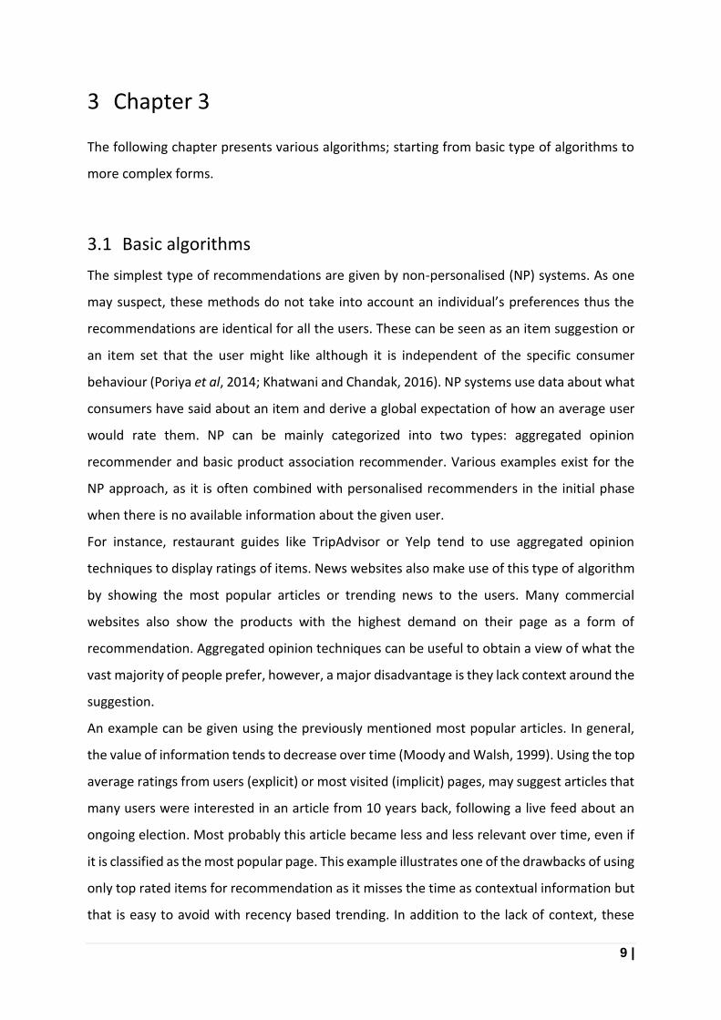
5.1.1.1 Weighted scheme

A weighted scheme combines the predictions of two or more recommender systems by

computing weighted sums of their respective scores.

Figure 4 – Weighted scheme (Brusilovsky et al, 2007)

In order to estimate weights, one may use an ensemble learning techniques like bagging or

any other empirical bootstrapping methods to gain the optimal combination of the

recommenders.

5.1.1.2 Switching technique

The second strategy - the switching technique - requires an oracle that decides which

recommender’s output should be favoured in specific scenarios, depending on the user

profile and or quality of recommendation results.

29 |

Figure 5 – Switching technique (Brusilovsky et al, 2007)

For instance to overcome the cold/start problem a knowledge based and collaborative

switching hybrid could initially make knowledge based recommendations until enough rating

data are available.

5.1.1.3 Mixed strategies

The third strategy within the parallelization is the mixed hybrid approach, whereas the results

of various recommender systems are combined at the level of the user interface, in which the

results from different techniques are presented along each other.

Figure 6 – Mixed strategies (Brusilovsky et al, 2007)

30 |

Thus the recommendation result for user u and item i is a set of tuples, representing the score

of each constituting recommenders.

5.1.2 Pipelined approach

The second type of hybridization is the pipeline approach. In this strategy, the different

recommender systems are placed into a pipeline. This implementation follows stages

whereas the techniques are sequentially combined and the last module generates the final

recommendations.

Figure 7 – Pipelined approach (Brusilovsky et al, 2007)

As with the parallelized approach, the pipelined approach also has further variants similarly

to the parallelized approach, namely the cascade and the meta-level strategies.

5.1.2.1 Cascade hybrids

Following the cascade logic, the recommender component n, is limited to items that were

also recommended by the preceding recommenders.

Figure 8 – Cascade hybrids (Brusilovsky et al, 2007)

31 |

For this reason, the following component cannot add new items to the list, but can exclude

items. In case the sequential order is changed and the components remained unchanged, it

will not have any effect on the final recommended list of items. However, it can introduce

some changes in the ordering of the list of recommended items as it solely depends on the

last technique. This is a crucial attribute as the system can help in reducing the overall

variance since the possibly overfitted items would fall out from the chain. Although this is a

trade-off between variance and bias, as a bad performing component which contains

erroneous assumptions in the learning algorithm will introduce a significant bias in the overall

system’s recommendation capability.

Meta-level hybrids

In a meta-level hybridization design, one recommender builds a model that is exploited by

the principal recommender to make recommendations. A typical use for meta-level hybrids

can be a CB recommender that builds user models based on weighted term vectors, and a CF

identifies similar peers based on the previous results from the CB results but makes

recommendations based on ratings.

Figure 9 – Meta-level hybrids (Brusilovsky et al, 2007)

32 |

5.1.3 Monolithic design

Whereas the parallelization and pipeline approach consist of two or more components whose

result are combined in a certain way, the monolithic hybridization implements only one

recommendation system.

Figure 10 – Monolithic hybrids (Brusilovsky et al, 2007)

The monolithic approach integrates aspects of different recommenders’ strategies into a

single algorithm. The hybridization is "virtual" in a sense that features/knowledge sources of

different paradigms are combined. Monolithic design use only a single recommender system

that integrates multiple approaches by pre-processing and combining various knowledge

source like ratings and user demographics or explicit requirements into one learning

algorithm. The hybridization is achieved by a built-in modification of the algorithm to exploit

different types of inputs.

5.1.3.1 Feature combination hybrids

Figure 11 – Feature combination hybrids (Brusilovsky et al, 2007)

33 |

Feature combination techniques combine various features like users’ rating data with content

features of catalogue items, enabling the system to identify new hybrid features.

5.1.3.2 Feature augmentation hybrids

Figure 12 – Feature augmentation hybrids (Brusilovsky et al, 2007)

Feature augmentation is another approach for integrating several recommendation

algorithms. This design technique does not simply combine and pre-process several types of

input but also applies more complex transformations during processing. The output of a

contributing system augments the feature space of the actual recommender by pre-

processing its knowledge sources. This technique is more flexible and adds fewer

dimensions than the feature combination method.

5.1.4 Hybrid System Experiments

The hybrid recommendation approach can provide synergistic improvement compared to

simple basic recommendation algorithms.

According to the experimental results; hybrid systems showed dominance over basic

recommendation systems. This synergy was found under situations like with smaller session

34 |

size, sparse recommendation density. This result means that hybridization can conquer cold

start problem which was innate for some basic recommendation systems.

The study of Burke (2002) showed this synergy. Aslanian et al (2016) also proved that their

proposed hybrid solution could better deal with the cold-start problem than the state-of-art

algorithms. Wei et al (2017) empirically tested that tight coupling of CF approach and deep

learning neural network is feasible and very effective for cold start item recommendation.

Zhitomirsky-Geffet, et al (2017) also developed a hybrid approach by combining two or more

traditional similarity metrics such as Pearson correlation, log-likelihood and Tanimoto

coefficient to tackle several well-known problems including cold start item recommendation.

Several other studies have also been conducted hybrid recommendation experiments and

proved the effectiveness improvement of hybrid systems.

35 |

6 Chapter 6

6.1 Challenges

Today, several recommender systems have been developed for different domains however,

they are not precise enough to fulfil the information needs of users. Therefore, it is necessary

to build higher quality recommender systems. In designing such recommenders, designers

face several issues and challenges that need proper attention. The following section highlights

the main issues and challenges and presents new research papers and solutions towards fine-

tuned and high-quality recommender systems.

6.1.1 Cold start

The cold-start problem was already mentioned in the section of CB recommenders and CF

methods. This challenge can be divided into two categories; cold-start items and cold-start

users. The problem arises when a new user or a new item has been added to the system. In

case that happens a traditional collaborative algorithm cannot recommend a new item to the

users until some users rate it and also, new users are unlikely to be given good

recommendations, due to the lack of their rating or purchase history.

Various approaches have been developed to mitigate this problem. Most of the solutions

focus on, or are related to the sparsity issue, hence they are presented together in the next

section.

6.1.2 Sparsity

The sparsity problem is closely related to the cold start problem and most of the proposed

solutions address both challenges.

Sparsity arises from the fact that most of the online systems contain thousands or millions of

items and even the most active users will only rate a few of the total number of available

items. The rating data then contains only minimal number of pairs between item (I) and user

(U), making the utility matrix sparse. High sparsity creates enormous challenge to achieving

high quality recommendations, as well as to the number of predictions that the systems is

able to compute.

36 |

The possible number of item predictions can be measured with the coverage metric, which is

defined as the percentage of items that has been rated and the percentage of items that each

algorithm could provide recommendations for. As nearest neighbour algorithms rely on exact

matches, the result is poor coverage and accuracy.

Several methods have been introduced to address the cold start and the data sparsity

problems. Most of the proposed methods to address item cold-start adopt content-based

approach; they utilize the content of new items in order to identify similar user profiles and

subsequently recommend these new items to them.

Content supported hybrid CF algorithms can address the sparsity problem as they do not rely

solely on user ratings. These approaches often use external content information which can be

used to produce predictions for new users and items.

Yuan et al (2016) propose a deep learning based matching algorithm to solve cold-start and

sparsity problems in CF based recommendation systems without major changes in the existing

system. Jian Wei et al developed a similar approach, using a hybrid recommendation model

to address the cold start problem, which explores the item content features learned from a

deep learning neural network and applies them to the time SVD++ CF model. Kim et al (2012)

published a paper about hybrid recommenders based on user similarity and content boosted

recommenders used in conjunction with interaction-based collaborative filtering to address

the cold start and sparsity problems in this domain.

External information can also be related to the user, external social information. Shaghayegh

et al (2011) presented a solution which use social networks’ information in order to fill the

gap and detect similarities between users. In this community based solution, features were

extracted from different dimensions of social networks to help recommendation

systems in solving cold-start problem based on the found latent similarities. Li and Tang

(2016) investigated how to provide a recommendation to a new user, based on a previous

group of user opinions, by utilizing techniques from social choice theory. Social choice theory

has developed models for aggregating individual preferences and judgments, so as to reach a

collective decision. In socially aware systems, user benefit from their trust and connections

with others as they can find other peers, those who they trust. Pitsilis and Knapskog (2012)

demonstrated an approach which used trust to exploit the latent relationships between users.

37 |

In this way, the opinions of distant participants can be discovered and used by users who do

not need to be known to each other.

6.1.3 Diversity and serendipity

Accuracy is a crucial part of recommender systems but chasing the accuracy curve may not

always be the right call. In the recent years, the focus of RS research has shifted to such

objectives as ensuring the suggested items are novel and the recommended population is

diverse. In a real life system people tend to like divers recommendations which help them to

discover something relevant but not expected. Therefore it is crucial to make sure set of

recommended items are as interesting and engaging as possible.

Increasing serendipity can be the key to increase novelty and positive discovery from the

users. The meaning of serendipity can be described as “happy and unexpected discovery by

accident” (Kaminskas and Bridge, 2014, p.1), originated from the 18th century. Serendipity

can be described as a surprise, delight in a sense that something unexpected resulted. It is

commonly agreed that serendipity consists of two components – surprise and relevance.

Meanwhile relevance is fairly easy to measure user ratings or any other feedback from the

users, surprise of recommendations is difficult to capture, as the notion of an item being

unexpected is difficult to measure without explicitly asking the users for their opinion.

There are several formulae which try to capture and quantify serendipity itself. The key

concept is the need of prior primitive estimate of obviousness, one such metric that

represents overall popularity of an item. Intuitively, by downgrading items that are highly

popular, one can increase serendipity. Therefore our intuition would say that an increase in

serendipity will lead to higher diversity. On the other hand, correctness dictates more

constraint which leads to a decrease in serendipity.

The results of Kaminskas and Bridge (2014) validate the former intuition that a MF approach

which tends to provide more accurate suggestions leads to less surprising ones, meanwhile a

user-based neighbourhood approach performs better in terms of surprise. (Murakami et al,

2008)

38 |

6.1.4 Scalability

As RS are designed to help users navigate in large collections of items, one of the most

important goal of such is systems is to scale up to real datasets.

When numbers of existing users and items grow tremendously, traditional CF algorithms will

suffer serious scalability problems, with computational resources going beyond practical or

acceptable levels. However, certain memory-based CF algorithms, such as the item-based

Pearson correlation CF algorithm can achieve satisfactory scalability. Traditional CF algorithms

calculate similarities between all pairs of items which is a bottleneck in such systems. Instead

of using a brute force, all pairs approach, item based Pearson CF calculates the similarity

between the pair of co-rated items by a user. This is especially beneficial in case the rating

matrix is sparse (which is generally the case).

Model-based CF algorithms, such as clustering algorithms, address the scalability problem by

partitioning users within a smaller and highly similar cluster, and using this and neighbouring

partitions for predictions. Meanwhile the computation complexity decreases the prediction

quality may decrease as well. It is worth noting that there are trade-offs between scalability

and prediction performance.

Dimensionality reduction techniques such as SVD can deal with the scalability problem and

quickly produce good quality recommendations, but they have to undergo expensive matrix

factorisation steps. This expensive step can be iterated in a Hadoop environment using

distributed computation. An incremental dimensional reduction algorithm precomputes the

decomposition offline, using existing users and items. After certain amount of new ratings or

users have been added to the database, the algorithm is able to update the existing system

without re/computing the low dimensional model from scratch. This second epoch takes

place online. Thus it makes the recommender system highly scalable.

39 |

7 Chapter 7

7.1 Evaluating recommender systems

There are many different recommender systems, serving diverse purposes. For this reason a

unified general evaluation strategy does not exist which would apply to all the problems. To

find the optimal solution for a specific problem, the results have to be evaluated with task

specific quantitative evaluation techniques. Not only the applied algorithm and recommender

technique can differ, but also the overall aim of the recommender system.

Therefore, this multi-faceted characteristic of recommendation systems lead us to consider

multiple dimensions for recommender evaluation such as correctness, coverage, diversity,

novelty, serendipity, robustness, learning rate, usability, scalability or stability. (Shanni and

Gunawardana, 2011)

● Correctness aims to measure the similarity between the predicted recommendations

and the previously assumed correct recommendations.

● Coverage is the set of items or user space the recommendation system can

recommend out of the total number of items or users.

● Diversity stands for how diverse are the recommended items in a list.

● Novelty is the system’s ability to recommend items that are new or to recommend

items to unknown users.

● Serendipity as an evaluation dimension is defined as how successful the system is in

providing surprising yet beneficial recommendations.

● Robustness is the system tolerance level towards bias or false information.

● Learning rate stands for how fast can the system incorporate new information to

update its recommendation list

● Usability dimension is about the user effort to adapt to the new system

● Scalability stands for measuring the algorithm performance; how scalable the system

is with respect to the number of users

40 |

The table below summarises the main measures that can be used to evaluate the

recommender systems by the specified dimensions.

7.1.1 Measures

Dimension Metric/Technique

Correctness

Ratings: Root Mean Square Error (RMSE), Normalized RMSE

(NRMSE), Mean Absolute Error (MAE), Normalized MAE

(NMAE)

Quantitative

Ranking: Normalized Distance-based Performance Measure

(NDPM), Spearman correlation, Kendall correlation, Normalized

Discounted Cumulative Gain (NDCG)

Classification: Precision, Recall, False Positive Rate, Specificity,

F-Measure, Receiver Operating Characteristics (ROC)

Coverage

Catalogue Coverage, Weighted Catalogue Coverage, Prediction

Coverage, Weighted Prediction Coverage

Diversity

Diversity Measure, Relative Diversity, Precision-Diversity Curve, Q-

Statistics, Set theoretic difference of recommendation lists

Novelty

Comparing recommendation list and user profiles, Counting

popular items

Serendipity Comparing recommendation list and user profiles, rateability

Robustness Prediction shift, average hit ratio, average rank

Learning rate Correctness over time

Usability User studies (survey, observation, monitoring)

Scalability Training time, recommendation throughput

Stability Prediction shift

Table 1 – Evaluation metrics (Avazpour et al, 2014)

41 |

7.1.2 Methodology

The methodology for evaluating the selected interest dimension can be online or offline

experiments. Online experiments run large scale experiments on a deployed system, which

we call online experiments. These experiments are often called A/B testing, which evaluates

the performance of the recommenders on real users which are oblivious to the conducted

experiment. The easiest measures for online evaluation is the Click-Through Rate (CTR) and

the conversion rate (CR) of the recommendations. It is worth pointing out that in some cases,

such experiments are risky. For instance a test system that provides irrelevant

recommendations, may discourage the test users from system ever again. Thus, the

experiment can have a negative effect on the system, which may be unacceptable in

commercial applications.

In most cases the only accessible and acceptable approach is to perform offline experiments

using existing data sets and a protocol that models user behaviour to estimate recommender

performance measures such as prediction accuracy. Offline evaluation typically uses split-

validation techniques based on the historical data.

This chapter has presented a range of dimensions and metrics which are used for the

evaluation of a recommender system. Also covered the different evaluation methodologies

and evaluation strategies for explicit and implicit ratings. Based on this, the practical part will

introduce the evaluation metric that the paper has used for the job recommendation problem

(Shani and Gunawardana, 2011).

42 |

8 Chapter 8

In this section we present our solution for the RecSys Challenge 2016.1 The Recsys Challenge

- as it was mentioned in the beginning - is an annual competition within the field of

recommender systems.

The challenge from 2016 was based on data provided by Xing.com2; a platform designed for

business networking, finding new job opportunities or just to establish and document

networks of people that one may know and trust professionally. On this website users can

interact with job posting and apply for positions.

8.1 Problem formulation

The challenge can be described as follows: given the profile information of the users, the

content of job postings and the historical log of each user's activities, predict a ranked list of

items that a set of target users will positively interact with, within the following week. Quality

metrics such as serendipity and novelty are not taken into account.

This particular business domain requires fast actions. An algorithm which requires hours or

even days to generate recommendations after a new user interact with the system, can

potentially lead to loss of information value. Therefore, the aim of our experiments is to

propose an efficient and scalable solutions for the job recommendation problem and also to

be able to react quickly after a new interaction has been inserted into the system.

Scalability is not just about speed. It has an important characteristic that the memory of the

program is bounded independent of data. For instance, it can mean that a dataset is not

completely loaded into memory before starting a learning process or feature engineering.

Vowpal Wabbit (Agarwal et al, 2011; VW github), an open source, fast out-of-core learning

system library originally developed at Yahoo! Research and currently being developed at

Microsoft Research, gives the definition of scalability in machine learning as: “There are two

ways to have a fast learning algorithm: (a) start with a slow algorithm and speed it up, or (b)

build an intrinsically fast learning algorithm. This project is about approach (b), and it’s

reached a state where it may be useful to others as a platform for research and

1 http://2016.recsyschallenge.com/; https://github.com/recsyschallenge/2016 2 https://recsys.xing.com/

43 |

experimentation”. Other researches (Paliouras, 1993, p.10 also see at Krueger et al, 2015)

define scalability as the linear increase in resources required, following a linear increase in

the requested output.

Both definitions can be interpreted as having learning algorithms that can manage any kind

of datasets, without consuming ever growing, exponential amount of resources, like memory.

Thus we can conclude that the algorithmic part of the solution is crucial, but this can also be

enhanced by having a distributed parallel solution which can execute iterative task with

increased speed.

The following sections are sentenced to provide details about our solution. Apart from

describing the main steps of developing the recommender system, the used technology side

is also briefly covered. In order, the section covering technology is presented first, followed

by that which describes data exploration and model training.

8.2 Used technology

The whole project makes use of distributed memory and the abstraction layer of Apache

Spark to help in implementing the machine learning algorithms for recommendation engine

and processing vast amount of data in reasonable time. Spark has an extensive set of

developer libraries and APIs; it also has a comprehensive support for various languages such

as Java, Python, R and Scala. The use of Hadoop environment and Spark enabled us to use the

framework for data ingestion, data processing, data exploration and visualisation, and

modelling the recommender task.

Spark has a concept of distributed memory abstraction which is called as Resilient Distributed

Dataset, which helps in reducing the disk writes and promotes the in-memory data processing

(Spark, 2016). Spark tries to keep things data iteratively in memory, whereas other big data

technicques like MapReduce involves more reading and writing from disk.

Although Spark’s performance advantage over MapReduce is known, Juwei Shi et al ’s paper

presents an in-depth analysis for performance differences between the two frameworks.

They executed various experiments using well known techniques such as Word Count, k-

means and PageRank algorithms. Generally, these experiments consisted a data read and

write process from an HDFS file for a mapper which was written to and from a SequenceFile

44 |

in between, before being written to an output file from a reducer. When the chain of multiple

jobs were needed, Spark executed the process flow much faster.

The paper also quantifies this advantage, stating that Spark is approximately 2.5x, 5x, and 5x

faster than the counterparts MapReduce for Word Count, k-means, and PageRank,

respectively.

Spark's ability to store data in memory and rapidly run repeated queries makes it well-suited

to train machine learning algorithms. Running broadly similar queries again and again at scale,

significantly reduces the required time to iterate through a set of possible solutions to find

the most efficient set of parameters. In ideal scenarios, it can be up to 100 times faster than

MapReduce. Based on these studies and results, we have decided to use Spark for this

particular problem.

After assessing the technology side, the next chapter summarises the main steps in

formulating the final solution.

8.3 Description of data

The provided datasets consist of four datasets - information about users, items, interactions

and impressions. The transactions time interval is from 19th August 2015 and 9th November

2015.

Users - 1.5M users

The dataset contains detailed user profiles. The attributes for the users are: career level,

discipline, industry, country, region, job roles, experience entries class, experience years in

total, experience years in current, educational degree and field of studies.

Items - 1.3M items

The set of items have common attributes to the users set, for example: career level, discipline,

industry, country, and region.

Interactions - 8.8M events

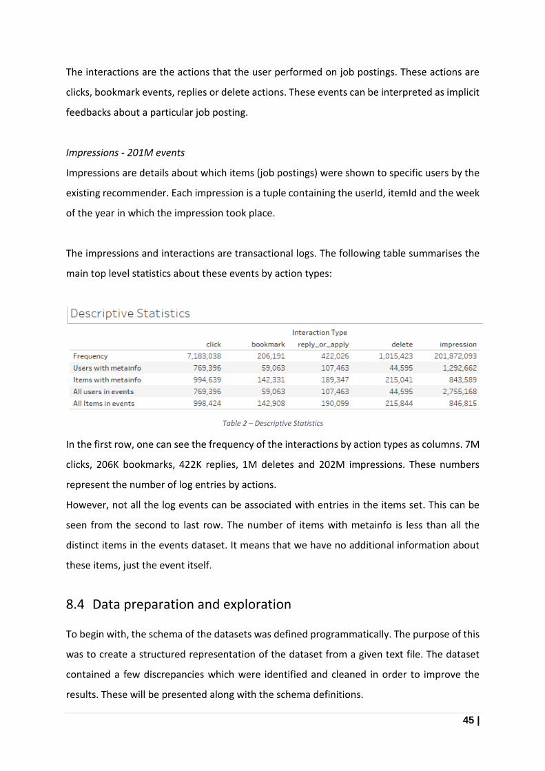
45 |

The interactions are the actions that the user performed on job postings. These actions are

clicks, bookmark events, replies or delete actions. These events can be interpreted as implicit

feedbacks about a particular job posting.

Impressions - 201M events

Impressions are details about which items (job postings) were shown to specific users by the

existing recommender. Each impression is a tuple containing the userId, itemId and the week

of the year in which the impression took place.

The impressions and interactions are transactional logs. The following table summarises the

main top level statistics about these events by action types:

Table 2 – Descriptive Statistics

In the first row, one can see the frequency of the interactions by action types as columns. 7M

clicks, 206K bookmarks, 422K replies, 1M deletes and 202M impressions. These numbers

represent the number of log entries by actions.

However, not all the log events can be associated with entries in the items set. This can be

seen from the second to last row. The number of items with metainfo is less than all the

distinct items in the events dataset. It means that we have no additional information about

these items, just the event itself.

8.4 Data preparation and exploration

To begin with, the schema of the datasets was defined programmatically. The purpose of this

was to create a structured representation of the dataset from a given text file. The dataset

contained a few discrepancies which were identified and cleaned in order to improve the

results. These will be presented along with the schema definitions.

46 |

Users schema

The users table originally contained 1.5 million users. The sanity check showed that not all the

user were unique, therefore the duplicated users had to be removed. After cleaning, the

unique number of users stood at 1,367,057; 91% of the original table. All of the user attributes

represented anonymized data.

Defined schema:

|-- id: integer

|-- jobroles: string:

❖ comma-separated list of job role terms (numeric IDs) that were extracted from the user's current job title. 0 means that there

was no known jobrole detected for the user.

|-- career_level: integer

❖ career level ID (e.g. beginner, experienced, manager)

|-- discipline_id: integer

❖ anonymized IDs represent disciplines such as "Consulting", "HR", etc.

|-- industry_id: integer

❖ anonymized IDs represent industries such as "Internet", "Automotive", "Finance", etc.

|-- country: string

❖ describes the country in which the user is currently working:

|-- region: integer

❖ Describes the region for some users (only within Germany)

|-- experience_n_entries_class: integer

❖ identifies the number of CV entries that the user has listed as work experiences

|-- experience_years_experience: integer

❖ is the estimated number of years of work experience that the user has

|-- experience_years_in_current: integer

❖ estimated university degree of the user

|-- edu_degree: integer

❖ estimated university degree of the user:

|-- edu_fieldofstudies: integer

❖ comma-separated fields of studies that the user studied. Entries refer to broad field of studies such as Engineering, Economics

and Legal etc.

Most of the users are located in Germany, Switzerland and Austria.

47 |

Figure 13 – Users registered location

One might expect a user to prioritise their interest in those roles posted closer to their current

location. However, in a considerable number of cases, users interacted with items that were

further away than their neighbouring regions.

Items schema

The items dataset contains rich meta information about job postings. No duplications were

identified in the item set.

Defined schema

|--id: integer

|-- title: string

|-- career_level: integer

|-- discipline_id: integer

|-- industry_id: integer

|-- country: string

|-- region: integer

|-- latitude: integer

|-- longitude: integer

|-- employment: integer

|-- tags: string

|-- created_at: integer

|-- active_during_test: boolean

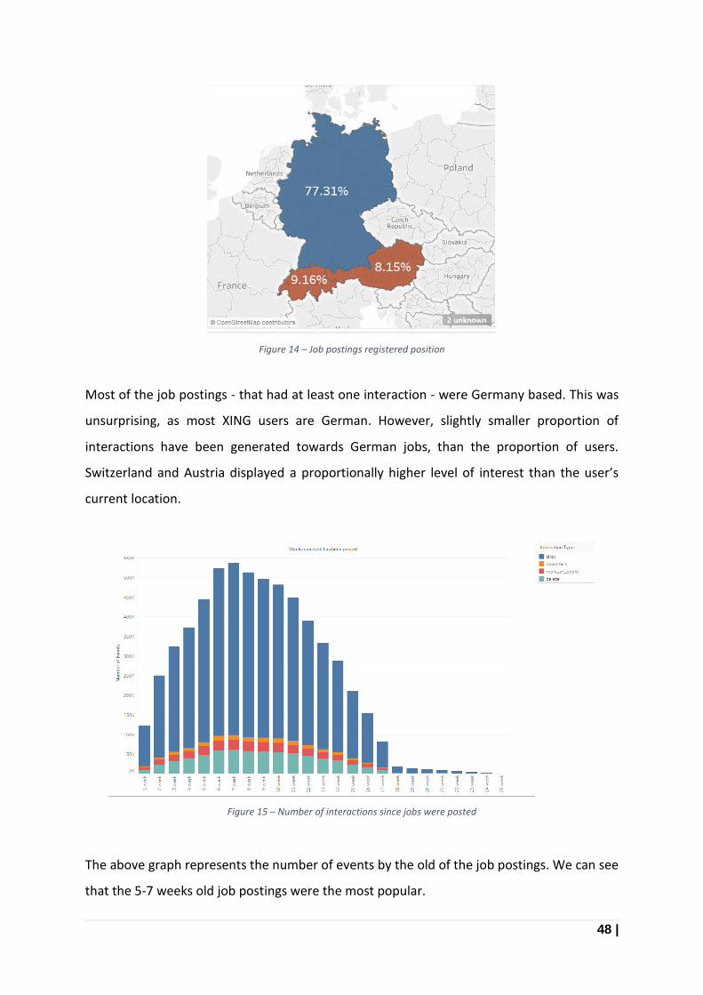
48 |

Figure 14 – Job postings registered position

Most of the job postings - that had at least one interaction - were Germany based. This was

unsurprising, as most XING users are German. However, slightly smaller proportion of

interactions have been generated towards German jobs, than the proportion of users.

Switzerland and Austria displayed a proportionally higher level of interest than the user’s

current location.

Figure 15 – Number of interactions since jobs were posted

The above graph represents the number of events by the old of the job postings. We can see

that the 5-7 weeks old job postings were the most popular.

49 |

Events schema

The raw impressions and interactions tables were transformed into a similar structure and

appended into a common data collection which was named as events table.

Defined schema:

|-- user_id: integer

|-- item_id: integer

|-- interaction_type: integer

❖ 0 - impressions

❖ 1 - clicks on job postings

❖ 2 - bookmarks

❖ 3 - replies, indicating that users intended to apply for the job

❖ 4 - deletes which corresponds to removing an item that the user no longer wants to see

|-- created_at: integer - unix timestamp

|-- cnt: integer - Number of interactions

Originally, the impression dataset itself did not contain an exact datetime for the specific

event; just the specific week of the year. Therefore the available week information was

allocated uniformly to each Wednesday of the particular week of the year. Also, the user-

item-week tuple for impressions were summarised and stored as the number of interactions.

These impressions were defined as the part of the list of items that an existing recommender

system had shown to the users (not all the recommended items were available). There is no

guarantee that the item was indeed a preferred item for the user.

On the contrary, interactions are user actions which can be used with higher confidence. An

average user clicked on 5.5 different job offers, which means that “click” is the most general

interaction type.

Figure 16 – Average number of interactions

The underlying distribution shows that there are thirty-seven thousand users who did not

have any interactions during the 5 months period. These users were treated as cold starters.

50 |

Figure 17 – Account’s event interactions

8.5 Challenges

8.5.1 Cold-start problem

As it has been pointed out, there were users that had had no activity (interactions) or even

impressions over the training period, but had already had in the test phase. For these users,

only some basic profile information might be available, without links to specific job items.

However, content based techniques could have faced difficulties if the user profile defined a

generic discipline or industry which applied to too many other users. In these cases, too many

job items might have been considered appropriate with the same level of estimated

confidence. The opposite could also have been a barrier, as an overly-specific profile could

have resulted in a limited number of matching jobs. Therefore, the solution needed to be able

to describe user and item segments without specifically categorising them into one cluster.

The proposed solution should would have been required to transform the available meta-

information into a latent space, in order to help to estimate interesting job offers for the

users.

51 |

8.5.2 Scalability

The system needed to be responsive and able to react to changes as fast as possible, due to

quickly-changing nature of the job-market. For each new users’ feature vector, the

representation was required to be updated swiftly, following each website interaction. This

could only be achieved if the solution was scalable and could be updated near real-time, with

online calculations.

8.5.3 Sparsity

1.363 million job postings were available in the given dataset. On average, users interacted

with 5.5 items during the 5 months timeframe which made the dataset extremely sparse. Our

task was to formulate a solution which used the given ratings that users have certain

interactions with and predicted their preference for the rest of the job items.

The number of unobserved ratings was substantial, thus traditional naive approaches could

be used for this problem.

A naive approach would have tried to estimate the ratings for each job posting for each user.

This would have led to a solution where the system estimated ratings for all items and users,

which would have meant 1.86 x 10¹² estimations. Also, transforming the ratings into a dense

rating matrix was not only not recommended, but likely unfeasible from a computational

perspective; it would have led to a huge 1.363M x 0.94M matrix.

In order to meet the scalability requirement, the model had to first find a way to reduce the

dimensionality.

8.6 Model training

Our study focused on developing an effective approach to making high-quality

recommendations, even when sufficient data was unavailable. Furthermore, the model would

be required to react quickly without needing to be retrained, whenever a new interaction

occurred in the system.

Our solution can be divided into three sections

1. Deriving latent topic segments from users meta information to provide

recommendations based on latent features and users’ feature distribution.

52 |

2. Scalable matrix factorisation solution utilising the power of Alternating Least Squares

technique.

3. Online feature vector creation for new users.

8.6.1 Latent user profile segments

The user dataset contained meta information about each users. Using this data it would be

possilbe to create new features and quantify relations between each entity.

Similarity between previous job roles or education should have brought two individuals

closer, but their profile may not have been exactly the same. Also, working in the same

industry with similar experience does not necessarily mean that the two individuals’ would

share the same interests.

Our approach was mainly driven by the fact that each individual belonged to a certain group

of people, each sharing a specific probability. Each user’s available information about their

previous job roles, discipline, degree, field of studies were transformed into a document

representation which described their own profile.

This text representation was further analysed and a latent model was fit to discover

underlying latent topics within the users, to segment them into semantically coherent parts.

A major benefit of using the proposed Latent Dirichlet Allocation (LDA) based approach was

the fact that each user had their own topic distribution with each underlying topic segment,

thus providing an implicit representation of the user’s profile. This profile helped us give a

higher weight for individual preferences and provides more personalised recommendation as

an explicit popularity based approach.

8.6.1.1 Deriving recommendations from latent topics

We utilised the extracted latent topic models to provide recommendations for the users.

53 |

Figure 18 – LDA technique to derive recommendations

Active users implicit ratings were used to aggregate opinions and distribute across latent

topics. Each latent topic was associated with a list of job postings which were the most

relevant for the specific segment. Next, the user’s topic distribution was used to redistribute

these preferences and calculate which job offers were potentially the most relevant, given

the user meta information. Each user had some sort of content information. By utilising the

content information of users, we were able to provide recommendations for users who didn’t

have any interactions in the system.

8.6.2 Alternating least squares

This approach utilises the power of the ALS matrix factorisation technique to model the job

recommendation problem.

We estimated a low-rank latent matrix factorisation representation of the ratings and users

to use the trained model to make predictions. The low rank representation was able to

uncover the latent factors that explained the observed user preferences towards job postings.

Each iteration attempted to find optimal weights to minimise the least squares between

predicted and actual ratings, whilst using a lambda regularisation to penalise complexity in

order to reduce the variance of the model.

54 |

In addition, the algorithm used an iterative approach, which leveraged Spark’s efficient

support for distributed computation.

Formula:

With each iteration, the algorithm fixed one factor in order to solve the equation for the

other. This process continued until the algorithm reached the predefined maximum number

of iterations. The optimal number of epochs was tuned based on convergence which will be

presented in the optimisation phase.

Figure 19 – ALS pseudo code

8.6.3 Recommending to existing and online updating for new users

The trained ALS model could provide recommendations for existing users only. The

recommendation was derived from the latent representations of users (u) and the job latent

factor matrix by multiplying the vector u and the matrix which scored the job postings. This

score gave us the ability to rank the items by users and evaluate them. The evaluation is

discussed in the next section.

55 |

Even though the model could not provide recommendations for users without interactions, it

was able to produce predictions for users whose first interaction had just occurred. The

method used the existing, trained model, without the need to recompute the latent matrix

and features. This was a crucial property, as it enabled the system to give personalised

recommendations to users who had no prior interactions.

The procedure differed between new and existing users, as the former did not initially have a

latent representation. The full item interaction vectors of existing users were used to compute

a similar latent representation for new users, by multiplying their corresponding full item

vector by the transpose of the latent job matrix. This allowed the method to compute

predictions for new users as soon as an interaction was received, using Spark streaming. This

did not require recalculation of the computationally more exhaustive model, which could be

instead scheduled offline after a certain period. For instance, the system could retrain and

trigger the ALS pipeline overnight, and during the day the algorithm could still produce

predictions for new users whose first interactions occurred during the day.

8.7 Evaluation methods

It is essential to emphasise that this problem was based on implicit feedback, and thus we did

not have reliable ratings for which job postings were not favoured. This is due to the

previously explained fact, that the lack of and interaction could arise from various reasons

and did not necessarily mean that a job posting was disliked. Although it would be reasonable

to assume that there were many instances of users neglecting to interact with job postings

due to lack of interest, it could also have been the case that it was not found. Traditional Root

Mean Square Error, or any other precision based metrics, would not have been suitable for

this problem, as they require the information about the non-favoured items. Even though we

may have been able to make the assumption that increased interactions was synonymous

with greater interest (and vice versa), implicit ratings cannot confirm this.

As the precision based evaluation technique was not appropriate in our case, a recall-oriented

approach was needed. The recommendation of each suggested methods could be interpreted

as an ordered list of items for user, where the top item is that which is predicted to be the

most preferred for the specific user. In order to evaluate these recommendations, we applied

56 |

a rank based evaluation, where the measure was based on each user's’ ordered interactions

(from the most interacted posts to the least).

If the rank score for a specific user u and specific item i was 0, it meant that the job post i was

predicted to be the most favoured by the user u. On the other hand, if this score was 1, it

indicated that the particular job post was likely the least desired for user u and thus placed at

the end of the list.

This formula described a minimisation problem and therefore the lower values for the

average rank evaluation were favoured, as they indicated that the ranking of actually

interacted job postings were closer to the top of the recommended lists.

8.8 Optimisation and training

The presented approaches contain parameters which can be tuned to gain higher

performance. The following section describes the optimisation process for both.

8.8.1 Latent topic approach

The first approach aimed to extract latent features from the user profiles. According to the

experimental results, the number of extracted topics did have an impact on the performance.

This solution identified similar neighbourhoods and used this knowledge to derive

recommendations without iterative training. For parameter tuning, we tuned the number of

latent topics, which were identified in the user profiles.

57 |

Figure 20 – Rank Score by latent topics

The model used the observed implicit ratings in the training set to identify the popular items

for each topic. The more topics that were available, the more granularity we gained. However,

we also introduced additional complexity and computation costs.

The results show that the evaluated rank score decreased monotonically as the number of

latent topics increased. This means that as the user profiles became more and more specific

to a particular user segment, it was able to utilise the additional knowledge and increase the

quality of the recommendations. However, after a certain point (around 100 latent topics),

the decrease slowed and it did not lead to significant improvement in the evaluated score. It

is possible due to the fact that additional latent topics are highly correlated and they cannot

separate further the users, thus resulting in similar top ranked items.

In evaluating the results, we decided to select 100 latent topics from the best performing

experiment. In this way, the model reached 0.36754 rank score on the training and 0.41415

on the test set.

8.8.2 Alternating least squares

In order to optimise the second technique, it required to tune more parameters in order to

reach the best results.

The implementation allowed us to estimate the parameters using grid search with cross

validation. The hyperparameter tuning was conducted using a 3 fold-cross validation on the

training set.

58 |

The model optimisation process was driven by the following parameters:

● Lambda, which controls the regularisation in the formula. Increasing this value may

have increased bias but decreased variance.

● Iterations, which is the number of maximum iterations the algorithm alternated

between both user and item feature vectors.

● Alpha, which is a parameter responsible for the baseline confidence in the observed

implicit rating values. It is associated with the confidence matrix, where

, thus, decreasing this would decrease the variability in

confidence between various ratings.

● Rank, which is the number of latent factors in the model.

8.8.2.1 Lambda, the regularisation parameter

The optimisation began by testing the regularisation parameter lambda (λ). The λ is

responsible for penalising complex solution, thereby reducing variance. This ensures the

generalisability of our model, helping to control the overfitting phenomena. The graph below

shows the test and validation error using different lambda values.

Figure 21 – Rank score by regularisation parameter

One may note that a lower lambda value allows the model to learn the test data, instead of

extracting general features from the training process. This leads to overfitting. On the other

hand, a higher value introduces too much bias into the model, preventing it to find the optimal

solution. The empirical results showed, that the optimal choice of 0.05 as a λ parameter

59 |

performed the best, while fixing other parameters accordingly (10 latent features, 30

iterations, 10 alpha).

8.8.2.2 Iterations, the number of training epochs

Different iteration numbers were tested while other parameters were fixed (0.05 lambda

value, 10 latent features and 10 alpha value).

Figure 22 – Rank score by iterations

According to the figure, we can state that the rank score monotonically decreases. However,

the improvement diminishes gradually. After 30 iterations it slows significantly, allowing us to

conclude that the algorithm converges within 30 iterations.

Figure 23 – Computational costs by iterations

Also, it is worth pointing out that the algorithm’s computational costs increase linearly with

respect of the number of iterations.

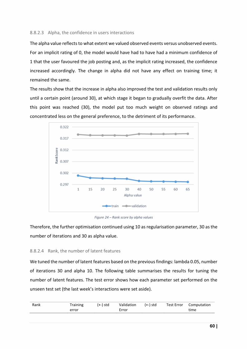
60 |

8.8.2.3 Alpha, the confidence in users interactions

The alpha value reflects to what extent we valued observed events versus unobserved events.

For an implicit rating of 0, the model would have had to have had a minimum confidence of

1 that the user favoured the job posting and, as the implicit rating increased, the confidence

increased accordingly. The change in alpha did not have any effect on training time; it

remained the same.

The results show that the increase in alpha also improved the test and validation results only

until a certain point (around 30), at which stage it began to gradually overfit the data. After

this point was reached (30), the model put too much weight on observed ratings and

concentrated less on the general preference, to the detriment of its performance.

Figure 24 – Rank score by alpha values

Therefore, the further optimisation continued using 10 as regularisation parameter, 30 as the

number of iterations and 30 as alpha value.

8.8.2.4 Rank, the number of latent features

We tuned the number of latent features based on the previous findings: lambda 0.05, number

of iterations 30 and alpha 10. The following table summarises the results for tuning the

number of latent features. The test error shows how each parameter set performed on the

unseen test set (the last week’s interactions were set aside).

Rank Training error

(+-) std Validation Error

(+-) std Test Error Computation time

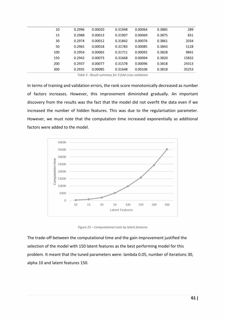
61 |

10 0.2996 0.00020 0.31948 0.00064 0.3885 289

15 0.2988 0.00013 0.31907 0.00069 0.3875 831

30 0.2974 0.00012 0.31842 0.00076 0.3861 2034

50 0.2965 0.00018 0.31783 0.00085 0.3843 5128

100 0.2954 0.00065 0.31711 0.00092 0.3828 9841

150 0.2942 0.00073 0.31668 0.00094 0.3820 15832

200 0.2937 0.00077 0.31578 0.00096 0.3818 24313

300 0.2935 0.00085 0.31648 0.00106 0.3818 35253

Table 3 - Result summary for 3-fold cross validation

In terms of training and validation errors, the rank score monotonically decreased as number

of factors increases. However, this improvement diminished gradually. An important

discovery from the results was the fact that the model did not overfit the data even if we

increased the number of hidden features. This was due to the regularisation parameter.

However, we must note that the computation time increased exponentially as additional

factors were added to the model.

Figure 25 – Computational costs by latent features

The trade-off between the computational time and the gain improvement justified the

selection of the model with 150 latent features as the best performing model for this

problem. It meant that the tuned parameters were: lambda 0.05, number of iterations 30,

alpha 10 and latent features 150.

62 |

8.8.3 Overall optimisation results

After evaluating all the parameters we can conclude that both approaches provided

reasonable results for the problem. The best training score using cross validation was reached

with the second method, train results of 0.3820. Meanwhile the first approach final score is

higher (0.41415), we must note that this technique is also able to provide recommendations

for users, who have not had any interactions with the platform, as it is based on the provided

user meta information. Therefore these methods could be used in parallel with each other

as a hybrid solution. Even though the second approach cannot provide recommendations for

users without interactions, after the first interaction the model is able to use these new

interactions and estimate further job preferences based on them.

63 |

9 Chapter 9

This chapter summarizes the main points of our thesis and concluding whether our

achievements have fulfilled the problem definition. Then, future work is presented.

9.1 Conclusions

The paper provided an overview about recommender systems with an introduction and

formal definition of these systems. It described various approaches from basic and heuristic

based recommenders to additional advanced model based techniques that the current state

of the art generally favours for specific problem formulations. We also discussed the issues

and challenges in developing recommender systems that needed special attention during the

practical implementation phase. The last chapter presented the job recommendation

problem and proposed scalable solutions. The problem definition from section 8 was stated

as follows:

“...given the profile information of the users, the content of job postings and the historical

log of each user's activities, the key task is to predict a ranked list of items that a set of

target users will positively interact with, within the following week. “

Our final solution consisted of two different recommenders which could be utilised for

different purposes. The first method used the user attributes and combined them into various

latent features which helped in identifying smaller segments. This solution was mainly driven

by the fact that each individual belongs to certain group of people with a specific probability.

The groups were formed by analysing and identifying certain latent topics between previous

job roles and position which helped quantifying the amount a user belonged to each one of

them.

The second method provided a latent factor algorithm that directly addressed the preference-

confidence paradigm. Even if the secondly proposed ALS model could identify personalised

recommendations with lower test scores the first model could be used in parallel to provide

recommendations for new users.

64 |

9.2 Future work

In this section we present issues which should be explored further to improve our

recommender system:

● Constraint based recommendations: The current implementation does not have any

constraints. However, it is more than likely that a job recommender platforms like

XING, does have important constraints; for example visa eligibility or the expiry of a

particular job posting.

● Contextual information: To further improve the system, we could have used additional

contextual information such as information describing time, users’ most recent

location area (not the registered location) and the items location to adjust the

recommendations. Also it would be interesting to enrich the job attributes with job

description and categorise jobs based on hidden features.

● Explanation to users: One limitation of our method is the way the neighbourhood style

explanation was generated, as it may not convey the reasoning behind the

recommendation. Therefore, the credibility of the system be improved with

explanations for recommended items.

● Further evaluation: Additional testing over a longer period of time would be beneficial,

with a larger variety of users. This could increase the confidence and show an overtime

performance of the model. When the users behaviours was analysed then the

measurements that would enable to assess the quality of the recommendations.

Based on those analyses appropriate improvements could be introduced.

● New Item problem: An important limitation must be pointed out, whereas job

postings without any interactions would not be recommended to users as potential

candidates with the current settings. Item content information could be used to solve

this problem.

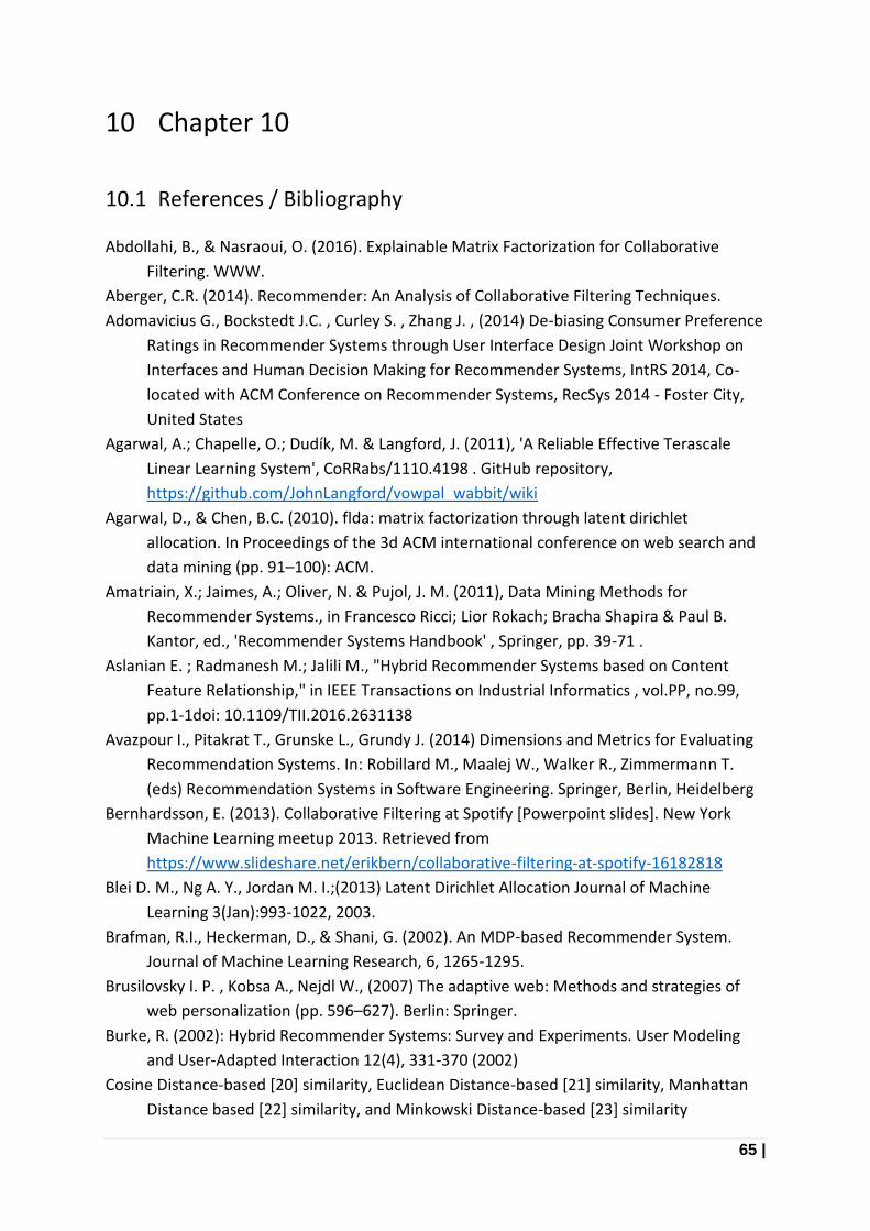
65 |

10 Chapter 10

10.1 References / Bibliography

Abdollahi, B., & Nasraoui, O. (2016). Explainable Matrix Factorization for Collaborative

Filtering. WWW.

Aberger, C.R. (2014). Recommender: An Analysis of Collaborative Filtering Techniques.

Adomavicius G., Bockstedt J.C. , Curley S. , Zhang J. , (2014) De-biasing Consumer Preference

Ratings in Recommender Systems through User Interface Design Joint Workshop on

Interfaces and Human Decision Making for Recommender Systems, IntRS 2014, Co-

located with ACM Conference on Recommender Systems, RecSys 2014 - Foster City,

United States

Agarwal, A.; Chapelle, O.; Dudík, M. & Langford, J. (2011), 'A Reliable Effective Terascale

Linear Learning System', CoRRabs/1110.4198 . GitHub repository,

https://github.com/JohnLangford/vowpal_wabbit/wiki

Agarwal, D., & Chen, B.C. (2010). flda: matrix factorization through latent dirichlet

allocation. In Proceedings of the 3d ACM international conference on web search and

data mining (pp. 91–100): ACM.

Amatriain, X.; Jaimes, A.; Oliver, N. & Pujol, J. M. (2011), Data Mining Methods for

Recommender Systems., in Francesco Ricci; Lior Rokach; Bracha Shapira & Paul B.

Kantor, ed., 'Recommender Systems Handbook' , Springer, pp. 39-71 .

Aslanian E. ; Radmanesh M.; Jalili M., "Hybrid Recommender Systems based on Content

Feature Relationship," in IEEE Transactions on Industrial Informatics , vol.PP, no.99,

pp.1-1doi: 10.1109/TII.2016.2631138

Avazpour I., Pitakrat T., Grunske L., Grundy J. (2014) Dimensions and Metrics for Evaluating

Recommendation Systems. In: Robillard M., Maalej W., Walker R., Zimmermann T.

(eds) Recommendation Systems in Software Engineering. Springer, Berlin, Heidelberg

Bernhardsson, E. (2013). Collaborative Filtering at Spotify [Powerpoint slides]. New York

Machine Learning meetup 2013. Retrieved from

https://www.slideshare.net/erikbern/collaborative-filtering-at-spotify-16182818

Blei D. M., Ng A. Y., Jordan M. I.;(2013) Latent Dirichlet Allocation Journal of Machine

Learning 3(Jan):993-1022, 2003.

Brafman, R.I., Heckerman, D., & Shani, G. (2002). An MDP-based Recommender System.

Journal of Machine Learning Research, 6, 1265-1295.

Brusilovsky I. P. , Kobsa A., Nejdl W., (2007) The adaptive web: Methods and strategies of

web personalization (pp. 596–627). Berlin: Springer.

Burke, R. (2002): Hybrid Recommender Systems: Survey and Experiments. User Modeling

and User-Adapted Interaction 12(4), 331-370 (2002)

Cosine Distance-based [20] similarity, Euclidean Distance-based [21] similarity, Manhattan

Distance based [22] similarity, and Minkowski Distance-based [23] similarity

66 |

Deerwester S., Dumais S. T. , Furnas G. W. , Landauer T. K., and Harshman R., “Indexing by

latent semantic analysis,” Journal of the American Society for Information Science, vol.

41, no. 6, pp. 391–407, 1990.

Di Noia, T., Mirizzi, R., Ostuni, V.C., Romito, D., Zanker, M.: Linked open data to support

content-based recommender systems. In: Proceedings of the 8th International

Conference on Semantic Systems, pp. 1–8. ACM (2012)

Funk S. (2006) Netflix Update: Try This at Home The Evolution of Cybernetics journal

Accessible http://sifter.org/simon/journal/20061211.html

G. Young and A. Householder. Discussion of a set of points in terms of their mutual

distances. Pages 19-22 of: Psychometrika, 3. 1938

Gemulla, R., Nijkamp, E., Haas, P. J., & Sismanis, Y. (2011). Large-scale matrix factorization

with distributed stochastic gradient descent (pp. 69–77). New York, New York, USA:

ACM. doi:10.1145/2020408.2020426

Goldberg K., Roeder T., Gupta D., and Perkins C.. (2001) Information Retrieval, 4(2), 133-151.

July 2001. Current site available from: http://eigentaste.berkeley.edu/

Gower J.C., Euclidean distance geometry The Mathematical Scientist, Vol. 7 (1982), pp. 1-14

Guan X., Li CT., Guan Y. (2016) Enhanced SVD for Collaborative Filtering. In: Bailey J., Khan L.,

Washio T., Dobbie G., Huang J., Wang R. (eds) Advances in Knowledge Discovery and

Data Mining. PAKDD 2016. Lecture Notes in Computer Science, vol 9652. Springer,

Cham

Gupta, P., Goel, A., Lin, J., Sharma, A., Wang, D., Zadeh, R.: Wtf: the who to follow service at

twitter. In: Proceedings of the 22nd International Conference on World Wide Web

Conference (2013), Rio De Janeiro, Brasil (2013)

Hu Y. , Koren Y. and Volinsky C. , "Collaborative Filtering for Implicit Feedback Datasets,"

2008 Eighth IEEE International Conference on Data Mining, Pisa, 2008, pp. 263-272.

doi: 10.1109/ICDM.2008.22

Iwata, T., Sawada, H., & Wanatabe, S. (2011). Fashion Coordinates Recommender System

Using Photographs from Fashion Magazines. IJCAI.

Jin H., Zhang L., Du L. (2013) Semantic Title Evaluation and Recommendation Based on Topic

Models. In: Pei J., Tseng V.S., Cao L., Motoda H., Xu G. (eds) Advances in Knowledge

Discovery and Data Mining. PAKDD 2013. Lecture Notes in Computer Science, vol

7819. Springer, Berlin, Heidelberg

Jurafsky, D., Martin, J. H. (2000), Speech and language processing : an introduction to

natural language processing, computational linguistics, and speech recognition ,

Pearson Prentice Hall , Upper Saddle River, N.J. .

Kaminskas M., (2014) 20 D., Measuring surprise in recommender systems, in: Proceedings of

the Workshop on Recommender Systems Evaluation: Dimensions and Design

(Workshop Programme of the 8th ACM Conference on Recommender Systems), 2014.

Kaminskas M., Bridge D. (2014): Measuring Surprise in Recommender Systems Workshop on

Recommender Systems Evaluation: Dimensions and Design (REDD 2014) at ACM

RecSys 2014,

67 |

Khatwani S. and Chandak M. B. (2016), "Building Personalized and Non Personalized

recommendation systems," 2016 International Conference on Automatic Control and

Dynamic Optimization Techniques (ICACDOT), Pune, 2016, pp. 623-628. doi:

10.1109/ICACDOT.2016.7877661

Kim M.W., Kim E.J., Ryu J.W. (2005) Collaborative Filtering for Recommendation Using

Neural Networks. In: Gervasi O. et al. (eds) Computational Science and Its Applications

– ICCSA 2005. ICCSA 2005. Lecture Notes in Computer Science, vol 3480. Springer,

Berlin, Heidelberg

Kim Y. S., Krzywicki A., Wobcke W., Mahidadia A., Compton P., Cai X. and Bain M. (2012)

Hybrid Techniques to Address Cold Start Problems for People to People

Recommendation in Social Networks DOI: 10.1007/978-3-642-32695-0_20

Koren Y., Bel R. l and Volinsky C., "Matrix Factorization Techniques for Recommender

Systems," in Computer, vol. 42, no. 8, pp. 30-37, Aug. 2009. doi: 10.1109/MC.2009.263

Krueger T., Panknin D., Braun M.,(2015): Fast Cross-Validation via Sequential Testing Journal

of Machine Learning Research, 16:1103-1155, 2015

Leeuw J.D.: (2006) "Nonlinear Principal Component Analysis and Related Techniques", 2006:

Greenacre, M. and Blasius, J. (eds), Multiple Correspondence Analysis and Related

Methods, Chapman & Hall/CRC Press, Boca Raton, USA. [GS 57] pp. 107-133

Li L., Tang X. (2016) A Solution to the Cold-Start Problem in Recommender Systems Based on

Social Choice Theory. In: Lavangnananda K., Phon-Amnuaisuk S., Engchuan W., Chan J.

(eds) Intelligent and Evolutionary Systems. Proceedings in Adaptation, Learning and

Optimization, vol 5. Springer, Cham

Lin, W., Alvarez, S.A. & Ruiz, C. Data Mining and Knowledge Discovery (2002) 6: 83.

doi:10.1023/A:1013284820704

Lü L., Medo M. , Yeung C. H. , Zhang Y.-C., Zhang Z.-K., and ZhouT. (2012), “Recommender

systems,” Physics Reports, vol. 519, no. 1, pp. 1–49, 2012.

Mahapatra, S., Tareen, A., & Yang, Y. (2011). A Cold Start Recommendation System Using

Item Correlation and User Similarity.

Manolis V. and Konstantinos G. M. (2004) Collaborative Filtering Enhanced By Demographic

Correlation, Department of Applied Informatics, University of Macedonia Egnatia 156,

P.O. 1591, 54006, Thessaloniki, Greece E-mail: {mans,kmarg}@uom.gr

Mika S., Schölkopf B., Smola A., Müller K. T., Scholz M., and Rätsch G.. 1999. Kernel PCA and

de-noising in feature spaces. In Proceedings of the 1998 conference on Advances in

neural information processing systems II, David A. Cohn (Ed.). MIT Press, Cambridge,

MA, USA, 536-542.

Min SH., Han I. (2005) Recommender Systems Using Support Vector Machines. In: Lowe D.,

Gaedke M. (eds) Web Engineering. ICWE 2005. Lecture Notes in Computer Science, vol

3579. Springer, Berlin, Heidelberg

Miyahara K., Pazzani M.J. (2000) Collaborative Filtering with the Simple Bayesian Classifier.

In: Mizoguchi R., Slaney J. (eds) PRICAI 2000 Topics in Artificial Intelligence. PRICAI

2000. Lecture Notes in Computer Science, vol 1886. Springer, Berlin, Heidelberg

68 |

Moody, D. L. & Walsh, P. (1999), Measuring the Value Of Information - An Asset Valuation

Approach., in Jan Pries-Heje; Claudio U. Ciborra; Karlheinz Kautz; Josep Valor; Ellen

Christiaanse; David E. Avison & Claus Heje, ed., 'ECIS' , Copenhagen Business School, ,

pp. 496-512 .

Mori K., Nguyen T., Harada T. and Thawonmas R., "An Improvement of Matrix Factorization

with Bound Constraints for Recommender Systems," 2016 5th IIAI International

Congress on Advanced Applied Informatics (IIAI-AAI), Kumamoto, 2016, pp. 103-

106.doi: 10.1109/IIAI-AAI.2016.244

Murakami T., Mori K., Orihara R. (2008) Metrics for Evaluating the Serendipity of

Recommendation Lists. In: Satoh K., Inokuchi A., Nagao K., Kawamura T. (eds) New

Frontiers in Artificial Intelligence. JSAI 2007. Lecture Notes in Computer Science, vol

4914. Springer, Berlin, Heidelberg

Nagarnaik P. and Thomas A., "Survey on recommendation system methods," 2015 2nd

International Conference on Electronics and Communication Systems (ICECS),

Coimbatore, 2015, pp. 1603-1608.doi: 10.1109/ECS.2015.7124857

Oord A. V. D., Dieleman S. and Schrauwen B. (2013) Advances in Neural Information

Processing Systems 26 (2013). 26.

Paliouras G. (1993) Scalability of Machine Learning Algorithms, Master's thesis, Department

of Computer Science, University of Manchester, (1993)

Pearlmuttery, B.A., & Parraz, L.C. (1996). A Context-Sensitive Generalization of ICA.

Pitsilis G, Knapskog S. J. (2012) Social Trust as a solution to address

Poriya A., Bhagat T., Patel N. and Sharma R.. Article: Non-Personalized Recommender

Systems and User-based Collaborative Recommender Systems. International Journal

of Applied Information Systems 6(9):22-27, March 2014.

Porsani M. J. , Silva M. G. , Melo P. E. M., Ursin B.. (2010) SVD filtering applied to ground-roll

attenuation. Journal of Geophysics and Engineering 7:3, 284-289. Online publication

date: 22-Jun-2010.

Pu P, Chen L, Hu R.(2011) A user-centric evaluation framework for recommender systems.

In: Proceedings of the fifth ACM conference on Recommender Systems (RecSys’11),

ACM, New York, NY, USA; 2011. p. 57–164.

RecSys Challenge 2016: http://2016.recsyschallenge.com/ ,

https://github.com/recsyschallenge/2016

Ricci, F., Rokach, L., Shapira, B.: Introduction to Recommender Systems Handbook. In: Ricci,

F., Rokach, L., Shapira, B. (eds.) Recommender Systems Handbook, pp. 1–35. Springer

(2011). DOI 10.1007/978-0-387-85820-3 1

Ricci F. and Nguyen Q. N. (2007), "Acquiring and Revising Preferences in a Critique-Based

Mobile Recommender System," in IEEE Intelligent Systems, vol. 22, no. 3, pp. 22-29,

May-June 2007.doi: 10.1109/MIS.2007.43

Rummel, R. J. (1970). Applied factor analysis. Evanston, IL: Northwestern University Press.

pp 227

69 |

Sarwar, B. M., Karypis, G., Konstan, J. & Reidl, J. (2002). Recommender Systems for Large-

Scale E-Commerce: Scalable Neighborhood Formation Using Clustering. Proceedings of

the 5th International Conference on Computer and Information Technology (ICCIT), .

Schafer J.B., Frankowski D., Herlocker J., Sen S. (2007) Collaborative Filtering Recommender

Systems. In: Brusilovsky P., Kobsa A., Nejdl W. (eds) The Adaptive Web. Lecture Notes

in Computer Science, vol 4321. Springer, Berlin, Heidelberg

Shaghayegh S. and William C., (2011) Community-Based Recommendations: a Solution to

the Cold Start Problem. In: Workshop on Recommender Systems and the Social Web

(RSWEB), held in conjunction with ACM RecSys’11, 23 October, 2011, Chicago.

Shani, G. & Gunawardana, A. (2011), 'Evaluating recommendation systems', Recommender

Systems Handbook , 257--297.

Shiau T.S., Cheng C.H and Tsai M. S. (2007) Application of Singular Value Decomposition

Technique to System Identification by Doping an Optimum Signal 中國機械工程學刊

第二十八卷第六期第605~616頁(民國九十六年) Journal of the Chinese Society of

Mechanical Engineers, Vol.28, No.6, pp.605~616(2007)

Sidorov, G; Gelbukh, A; Gomez-Adorno, H y Pinto, D.Soft Similarity and Soft Cosine

Measure: Similarity of Features in Vector Space Model. Comp. y Sist. [online]. 2014,

vol.18, n.3, pp.491-504. ISSN 1405-5546. http://dx.doi.org/10.13053/CyS-18-3-2043.

Spark, Spark Programming Guide (2016) Spark 2.0.0 Documentation, Spark.apache.org,

Accessible http://spark.apache.org/docs/2.0.0/programming-guide.html#resilient-

distributed-datasets-rdds

sparsity-inherent problems of Recommender systems .CoRR abs/1208.1004 (2012).

Tang, J., Hu, X. & Liu, H. Soc. Netw. Anal. Min. (2013) 3: 1113. doi:10.1007/s13278-013-

0141-9

Tellinghuisen, J. 2008. Least squares with non-normal data: Estimating experimental

variance functions. 2008 Feb;133(2):161-6. doi: 10.1039/b708709h.

Wang Z., Yu X., Feng N. and Wang Z. (2014) An improved collaborative movie

recommendation system using computational intelligence J. Vis. Lang. Comput. J. Vis.

Lang. Comput. Vol 25, pp 667 - 675

Wei, J, He, J, Chen, K, Zhou, Y & Tang, Z 2017, 'Collaborative filtering and deep learning

based recommendation system for cold start items' Expert Systems with Applications,

vol 69, pp. 29-39. DOI: 0.1016/j.eswa.2016.09.040

Wei S., Ye N., Zhang S., Huang X. and Zhu J., "Item-Based Collaborative Filtering

Recommendation Algorithm Combining Item Category with Interestingness Measure,"

2012 International Conference on Computer Science and Service System, Nanjing,

2012, pp. 2038-2041.doi: 10.1109/CSSS.2012.507

Yuan J., Shalaby W., Korayem M., Lin D., AlJadda K. and Luo J. (2016) , "Solving cold-start

problem in large-scale recommendation engines: A deep learning approach," 2016

IEEE International Conference on Big Data (Big Data), Washington, DC, 2016, pp. 1901-

1910.doi: 10.1109/BigData.2016.7840810

70 |

Zhitomirsky-Geffet M., et al, (2017), "Risk analysis and prediction in welfare institutions

using a recommender system", AI & SOCIETY, pp. , 2017, ISSN 0951-5666.

Zhou, X., He, J., Huang, G., Zhang, Y.: (2015)15 SVD-based incremental approaches for

recommender systems. J. Comput. Syst. Sci. 81(4) 713-733

Zhou Y., Wilkinson D., Schreiber R., Pan R. (2008) Large-Scale Parallel Collaborative Filtering

for the Netflix Prize. In: Fleischer R., Xu J. (eds) Algorithmic Aspects in Information and

Management. AAIM 2008. Lecture Notes in Computer Science, vol 5034. Springer,

Berlin, Heidelberg