a sampling model for validity

125

A Sampling Model for ValidityMichael T. KaneNational League for Nursing

A multifacet sampling model, based ongeneralizability theory, is developed for the mea-surement of dispositional attributes. Dispositionsare defined in terms of universes of observations,and the value of the disposition is given by the uni-verse score, the mean over the universe defining thedisposition. Observed scores provide estimates ofuniverse scores, and errors of measurement are in-troduced in order to maintain consistency in theseestimates. The sampling model provides a straight-forward interpretation of validity in terms of the ac-curacy of estimates of the universe scores, and of

reliability in terms of the consistency among theseestimates. A third property of measurements, im-port, is defined in terms of all of the implicationsof a measurement. The model provides the basis fora detailed analysis of standardization and of thesystematic errors that standardization creates; forexample, the hypothesis that increases in reliabilitymay cause decreases in validity is easily derivedfrom the model. The model also suggests an expli-cit mechanism for relating the refinement of mea-surement procedures to the development of lawsand theories.

1. Introduction

The technical quality of behavioral measurements is evaluated in terms of two properties-relia-bility and validity. Validity involves the interpretation of the observed score as representative of someexternal property, and reliability deals with the consistency among observed scores. In general terms,reliability is concerned with precision and validity is concerned with accuracy (Stallings & Gillmore,1971). Since a very precise estimate of the wrong attribute is less useful than a relatively imprecise es-timate of the intended attribute, validity is generally considered to be more important than reliability.However, the evidence for the validity of most behavioral measurements is less adequate than the evi-dence for their reliability. Ebel (196~) has aptly described this dilemma:

Validity has long been one of the major deities in the pantheon of the psychometrician. It is uni-versally praised, but the good works done in its name are remarkably few. Test validation, infact, is widely regarded as the least satisfactory aspect of test development. (p. 640)

This situation has not improved markedly since 1961. The statement often found in introductory text-books equating validity with the extent to which scores measure &dquo;what they are intended to measure&dquo;

Downloaded from the Digital Conservancy at the University of Minnesota, http://purl.umn.edu/93227. May be reproduced with no cost by students and faculty for academic use. Non-academic reproduction

requires payment of royalties through the Copyright Clearance Center, http://www.copyright.com/

126

provides an extreme example of the conceptual problems that surround validity, since it suggests theexistence of a &dquo;true&dquo; value for an attribute, without specifying what this 66true99 value represents.

Ebel (1961) has also pointed out that physics does not seem to encounter problems of validation.Indeed, in the classic analysis of physical measurement, Campbell (1957) did not employ a separateconcept of validity defined in terms of the relationship between observed values and &dquo;true&dquo; values. In

developing and evaluating measurement procedures for physical properties, such as length and mass,the interpretation of the properties is closely tied to the observations that are used in their measure-ment, and therefore validity is built into the measurements. Because the connection between the in-terpretation of physical attributes and their measurement is often particularly straightforward, sev-eral of the examples used in this paper will involve physical measurement.

The multifacet sampling model developed in this paper is based on generalizability theory (Cron-bach, Gleser, Nan da, & Rajaratnam, 1972). Although most of the results are stated in terms of vari-ance components, the development of the model emphasizes conceptual rather than technical issues.The most useful results of the sampling model deal with the questions that should be asked and thegeneral form of the answers that should be sought in analyzing measurements.

Measurements are analyzed by examining how observations are related to their intended inter-pretation. The model provides an analysis of reliability, validity, errors of measurement, the distinc-tion between random errors and systematic errors, standardization, and the role of theory in inter-preting measurement. Within the sampling model the issues of reliability, validity, and errors of mea-surement arise naturally as requirements for the intended interpretations to be meaningful. Since thedevelopment of the model’s implications is quite long, and, in some ways relatively convoluted, anoverview of the main points in the development may provide a useful road map.

Section 11 examines the interpretation of attributes as dispositions defined in terms of universes ofpossible observations. The value assigned to an attribute is defined as the expected value over thisuniverse, and measurements are interpreted as estimates of this expected value. Because the esti-mates are based on samples from the universe defining the attribute, the model is a sampling model.Estimates of the attribute’s value based on different samples will not generally be equal, and in orderto maintain consistency, an explicit theory of errors is introduced.

Section III provides a brief outline of generalizability theory and introduces a sampling model forvalidity. The validity of measurements of a dispositional attribute is defined in terms of the accuracywith which the observed scores estimate the expected value for the appropriate universe.

Section f’~ examines the effects of standardization on measurement procedures. Standardizedmeasurements involve two kinds of errors: random errors, which vary from one observation to an-

other, and systematic errors, which are constant for a series of observations. Reliability is associatedwith random errors, and validity is associated with systematic errors.

Section V explores the relationship between theory and measurement. A third property of mea-surement is introduced by defining the concept of import in terms of all of the inferences that can bedrawn from an observed score. Import is associated with the connotation of attribute labels, whilevalidity is associated with denotation of attribute labels. This section reviews some powerful tech-niques for controlling errors of measurement.

Finally, Section VI examines the assumptions underlying the sampling model and presents someconcluding comments. In particular, the problems associated with the sampling assumptions are dis-cussed within the broader context of the problem of inductive inference.

EL The Interpretation of Measurable Attributes

Lord and Novick (1968, p. 17) define measurement as &dquo;a procedure for the assignment of num-



127

bers ... to specified properties of experimental units in such a way as to characterize and preservespecified relationships in the behavioral domain.&dquo; According to Nunnally (1967, p. 2), 661~easurementconsists of rules for assigning numbers to objects to represent quantities of ~ttrib~teso’9 Campbell(1957, p~ 267) defines physical measurement as &dquo;the process of assigning numbers to representqualities.&dquo;

According to each of these definitions, measurement involves a functional relationship betweenreal numbers and the members of some class of objects. Depending on the attribute being considered,the objects may take a variety of forms, including physical objects, persons, and various complex sys-tems. The rules used to assign the numbers may also vary considerably. The process of measurement,however, always involves a mapping of object o into a real number, P., representing the value of theattribute for o. The fact that the number is assigned to the object of measurement involves a funda-mental theoretical commitment, in that it implies that the attribute depends only on the object ofmeasurement and does not depend on any other conditions that may prevail when the observationsare made. For example, the statement that the length of a metal bar is 1.5 meters treats length as aproperty of the bar and implies that length does not depend, for example, on the location, orientation,or temperature of the bar, or on the identity of the observer.

Attributes

There are at least three kinds of attributes in science (see Ellis, 1968): basic attributes, derived at-tributes, and theoretical attributes. This paper is concerned mainly with the measurement of basicand derived attributes, but theoretical attributes will also be discussed briefly under the heading ofconstruct validity,

A basic attribute represents an observed ordering on some property. It is noticed, for example,that some objects are easier to move than others and that this ordering of the objects remains thesame regardless of their location, who attempts to move them, or when they are moved. It is conven-ient, therefore, to think of &dquo;resistance to movement&dquo; as a property, or attribute, of the objects; and alarge class of solid objects can be characterized by this property. Where such an ordinal propertyexists for a class of objects, a basic attribute can be developed by assigning numbers to the objectscorresponding to their ordering. Basic attributes are generally the first kind of attribute developed ina science.

A basic attribute can always be viewed as a disposition, or a tendency, to produce a certain reac-tion to some test conditions (Carnap, 1953, 1966). Dispositions may be qualitative or quantitative. Fora qualitative d~,~~®~~t~®~z9 the object is said to have the attribute if and only if a specific reaction occursin the presence of appropriate test conditions. For example, an object is said to be a magnet if, whenplaced near a small piece of iron that is free to move (the test condition), it causes the iron to move(the reaction). For a quantitative disposition, a number is assigned to the object on the basis of thestrength of the reaction to the test conditions. The magnitude of the attribute of being magnetic, orthe strength of a magnet, can be defined in terms of the force it exerts on a piece of iron.

The basic attribute, mass, is derived from the qualitative ordering of objects in terms of their re-sistance to movement; and the measurement of ~n~ss9 using balances and springs, reflects this origin.In many cases, however, the procedures used to measure a basic attribute do not reflect the originalqualitative ordering so closely. The attribute temperature is based on the ordering of objects in termsof perceived warmth or coolness. The ordinary operations for measuring temperature, however, in-volve the expansion of liquids. Since it is known empirically that the volume of a liquid is closely re-lated to perceptions of warmth, and since measurements based on liquid thermometers have much



128

higher interobserver agreement than perceptions of warmth, thermometers have been substituted forperceived warmth in measuring temperature.

Derived attributes are constants in empirical laws (see 1950). After measurements of somebasic attributes are available, empirical laws stating relationships among the basic attributes may bedeveloped, and these laws often involve constants that can also be treated as measurable attributes.For example, the length of metal bars is found to depend on their temperature, and the empirical lawstating this relationship contains a constant, k, called the coefficient of thermal expansion of the bar.The value of k varies from one bar to another but remains relatively constant from one observation toanother on a given bar. It is convenient, therefore, to interpret k as a property of the bar by assumingthat it depends on the bar but not on the conditions prevailing when the bar is observed. The constantk is called a derived attribute because its interpretation depends on, or is derived from, the law relat-ing the basic attributes length and temperature.

Theoretical attributes are not directly observable but can be assigned a number indirectly be-cause of their connection, through a theory, to one or more observable attributes. It is sometimes pos-sible to explain a number of laws in terms of a few postulates defining a theory, and these postulatesgenerally involve theoretical attributes. Through the network of relationships constituting the theory,the theoretical attributes are connected to the basic and derived attributes that appear in the lawsthat the theory is designed to explain. The existence of the theory makes it possible to interpret ob-served scores on two levels. First, they may be interpreted as more-or-less direct estimates of a basic orderived attribute. Second, the same observations may be interpreted as indirect indicators of an un-observable theoretical construct.

Operational Definitions

The rules that are used to assign a value to basic and derived attributes are usually called oper-atioiial definitions (Bridgman, 1927). The rules are operational in the sense that they are stated interms of the operations performed in measuring the attribute. The rules are said to be definitions be-cause they provide an interpretation for the numbers assigned as values of the attribute (see Carnap,1953; Ennis, 1973; Hempel, 1960).

Operational definitions generally include two kinds of rules-structural rules and selection rules.The structural rules specify the kind of observations that are to be used and the way in which num-bers are derived from these observations. The structural rules may be more or less elaborate, but theyalways leave some issues open; for example, a particular observer would not be named. The selection,rules specify the range of conditions that may be tolerated for the various characteristics of the obser-vations. Some characteristics may be fixed, and some may be defined in terms of classes of conditions.lt is assumed that the characteristics not mentioned in the structural rules need not be controlled atall.

Operational definitions do not specify particular observations; they specify classes, or universes,of observations. The definition of an attribute can always be made more precise and more completeby specifying particular conditions of observation, but it would be impossible to specify all of thecharacteristics that might influence an observation. Operational definitions are designed to achievesome generality of application while providing a clear indication of the kind of observations allowed.The universe of observations specified by the definition is generally somewhat fuzzy, in the sense thatthere are marginal cases in which it is not clear whether the observation should be included in the uni-verse. This ambiguity is tolerated because it facilitates the development of scientific laws (Toulmin,



129

1953) and does not represent a serious problem in practice. It does, however, complicate the interpre-tation of sampling models, and these complications will be examined in the last section of this paper.

It is sometimes claimed that measurements of operationally defined attributes are valid by defini-tion. It is maintained that the operations used to measure the attribute define the attribute, and theresults of these operations are, by definition, the values of the attribute. According to this view, no in-terpretation is to be given to measurements beyond the fact that they result from particular opera-tions. In practice, however, the operational definitions of even the most narrowly defined attributesinvolve classes of observations rather than particular observations. No operational definition in sci-ence specifies a particular observer (John Jones), particular equipment (voltmeter No. 6), or a particu-lar time and place. If the results of a particular observation could not be interpreted in terms of a uni-verse of similar observations, these results would be of little interest. To assign a value to an attributeis to make a claim about a universe of observations.

Although restrictions may be placed on the qualifications of observers and on the type of equip-ment used, these restrictions define classes of observations rather than particular observations. Acomplete description of a single observation would require exhaustive specification of all of the condi-tions under which the observation is made. The definition of a dispositional attribute specifies onlysome of the conditions of observation, thereby allowing the other conditions to vary, and describes aclass of observations rather than a single observation. Since few of these observations will actually bemade for any object of measurement, the value of the attribute is inferred rather than observed.

Therefore, each observation provides information about a. universe of observations that could havebeen made. This generalization from particular observations to the universe defining an attribute is acardinal feature of measurement.

The Object of measurement

The object, or unit, to which a number is assigned by measurement is the object of iiieastiremeiit.The operational definition of an attribute specifies a class of observations for each object of measure-ment, and any of these observations could be used to estimate the value of the attribute for the objectof measurement. Also, each observation can provide information about different objects of measure-ment ; and if the measurement is to be interpreted unambiguously, the object of measurement mustbe clearly identified.

For example, in a study of anxiety, an observation might consist of the response of a person tosome stimulus in a particular context. For such observations, the person is usually considered to bethe object of measurement, and the level of anxiety is attributed to the person. In examining the de-gree to which various stimuli or contexts provoke anxiety, however, the objects of measurement wouldbe stimuli or contexts, respectively. More complicated objects of measurement can also be con-sidered. For example, the differential impact of stimuli on different persons could be described bytaking person-stimulus pairs as the objects of measurement; in this case, the attribute would indicatehow much anxiety the stimulus causes in the person. Cardinet, Tourneur, and Allal (1976) have dis-cussed how the interpretation of an observation depends on the definition of the object of measure-ment.

The specification of the object of measurement is a conceptual issue and is not uniquely deter-mined by the nature of the observations that are made. As the above examples illustrate, a single ob-servation can provide information about a variety of objects of measurement. Similarly, many differ-ent observations may be used to measure a particular attribute for an object of measurement. The set



130

of all possible objects of measurement for an attribute will be referred to as the population for the at-tribute.

The distinction that is often drawn in psychology between a state and a trait depends on a distinc-tion between different kinds of objects of measurement. If the object of measurement is considered tobe a person in a particular context, then the attribute being measured is a state variable, which is as-sumed to be a function of both the person and the time. It is expected that the value associated with astate variable will change as the context changes over time. For a trait, the object of measurement isthe person, and the value of the trait variable is assumed to be independent of time. It is recognized,of course, that the behaviors associated with the trait may be exhibited to different degrees in differ-ent contexts, but the value assigned to the trait is assumed not to change. For a trait variable, changesin the observed variable over time are treated as errors of measurement; for a state variable such dif-ferences are accounted for by differences in the value of the state variable.

In the physical sciences, distinctions among different kinds of objects of measurement are oftendrawn very carefully. In their introductory treatment of mechanics, Corben and Stehl (1960) state thefollowing assumptions:

A particle is described when its position in space is given and when the values of certain param-eters such as mass, electric charge, and magnetic moment are given. By our definition of a par-ticle, these parameters must have constant values because they describe the internal constitutionof the particle. If these parameters do vary with time, we are not dealing with a simple particle.The position of a particle may, of course, vary with time. (p. 6)

Therefore, the mass, charge, and magnetic moment are to be treated as trait variables, with particlesas their objects of measurement; position is to be treated as a state variable which varies over timeand therefore has particle-time combinations as its objects of measurement.

The Use of Invariance m Inferences Thickets

Attributes are &dquo;constructed&dquo; by specifying universes of observations. Measurements of attributesare based on samples from these universes. In order to interpret a measurement as the value of an at-tribute for the object of measurement, there must be generalization from a sample of observations toa universe of observations. A central concern of a theory of measurement is therefore the justificationof such inferences.

The evidence for a scientific inference is generally provided by appeal to laws (Hempel, 1965); andbecause the justification of inferences is their major function, Toulmin (1953) refers to scientific lawsas &dquo;inference tickets.&dquo; The type of law that is needed to justify the interpretation of observations asmeasurements is an invariance property. An Invariance property, or invariance law, states that the re-sults of a certain kind of observation do not depend on some of the conditions of observation. Invari-ance laws are needed for the interpretation of measurement because measurement assigns a value toan object of measurement and not to an observation.

The attribute is identified with a universe of observations and not with a particular observation.Any observation from this universe could be used to assign a value for the attribute to the object ofmeasurement. The observed score, Xoi, for an observation is the real number to the observa-tion by the structural rules for the attribute. A different but equally legitimate observed score, Xillcould be obtained by changing the conditions of observation in accordance with the selection rules.

When an observed score is interpreted as a measurement, it is assumed that this observed scorerepresents the value of the attribute for the object of measurement. Since different observations will



131

yield different observed scores for an object of measurement, the following relationship must hold, atleast approximately, in order to avoid inconsistency:

F ....I I

where and i’ represent any two observations that satisfy the definition of the attribute. That is, theobserved scores must be approximately invariant over the universe of observations defining the attri-bute. Since the two quantities in Equation 1 are observable, this assertion is testable for any pair ofobservations, and Equation I is an empirical hypothesis.

Equation 1 is an invariance law stating that the observed scores are invariant over the universe de-fining the attribute. For a given object of measurement, o, all observations included in the definitionof the attribute should assign the same value to the object of rne~sur~~r~~~t9 and if they do, this com-mon value may be taken to be the value of the attribute for the object of measurement, o. Note thatthe invariance properties required for the measurement depend on the definition of the attribute be-ing measured. If the two quantities in Equation awere not taken as measurements of the same attri-bute for the same object of measurement, there would be no reason to require that they should havethe same value.

Considering again the example discussed earlier, if anxiety is interpreted as a trait, the situationsin which observations are made are conditions of observation, and invariance over situations is as-sumed. If anxiety is interpreted as a state, the objects of measurement are persons in situations, andchanges in the attribute value as a function of the situation are consistent with this interpretation.

Invariance laws are involved in measurement because they justify inferences from samples of ob-servations to a universe of observations. If all of the observations in the universe give the same resultfor any object of measurement, then any one of these observations would provide complete informa-tion about the universe. If Equation 1 holds for all pairs of observations defining an attribute, it pro-vides the necessary justification for inferences from observed scores to the attribute value. To the ex-tent that observations fail to satisfy Equation 1, such inferences will be inconsistent (Suppes, 1974).Therefore, the invariance law in Equation I is necessary for the interpretation of observations as mea-surements of dispositional attributes.

Errors of Measurement

The inconsistency arising from violations of Equation 1 oan be eliminated by introducing the con-cept of an error of measurement. The result of any observation on an object, o, is taken to be the sumof the &dquo;true&dquo; value of the t09 plus an error of measurement, e,,i,

Since neither the &dquo;true&dquo; score nor the error is directly observable, Equation 2 is not a testable hypoth-esis ; rather, it is a definition of the error, eai.

However, the values assigned to the errors are not arbitrary. Given the universe defining an attri-bute and a value for the true score, the errors are determined empirically. If the observed scores haveapproximately the same value, the values assigned to the errors can be small. If the observed scores ona given object of measurement vary widely, the values assigned to the errors must be large. Small er-rors of measurement are, of course, generally perferred over large errors of measurement, and there-fore Equation 2 provides a relative criterion for evaluating measurement procedures.

Classical test theory defines the value of an attribute for an object of measurement as the ex-pected value over all observations included in the definition of the attribute. This choice is convenient



132

because it minimizes the mean-square error. With this definition of true score, it is easy to show thatthe expected value of the errors is zero for each object of measurement and, therefore, that the errorvariance for each object of measurement is equal to its observed score variance. Such object-specificerror variances are very useful because they indicate the accuracy of estimates of the true score foreach object of measurement,. However, the direct estimation of the object-specific error variance re-quires repeated observations on each object of measurement, and this is often not practical.

A more easily estimated parameter is the average error variance, 02 (e), over all objects of measure-ment. The average error variance is more widely used than the object-specific error variance becauseit can be estimated with pairs of observations on each object of measurement. The covariance be-tween true scores and errors of measurement can be shown to be zero, and therefore the observedscore variance can be partitioned as

where 62(t~ is the variance in the true scores over the population and o2(~~ is the average error vari-ance.

Errors of Measurement as Constructs

In the absence of assumptions about attributes and objects, the concept of an error of measure-meant is unnecessary. If attention is restricted to observations, there is no reason to reject the hypoth-esis that every observation is perfectly accurate. Suppose, for example, that two observers putthermometers into the same glass of water at the same time. Suppose further that one of the observersrecords the temperature as 20° C and the other observer records the temperature as 22° C. These twoobservations differ in several ways, for example, in terms of the observer, the thermometer, and theposition in the water. If the two numbers, 20 and 22, are assigned to the observations, there is no rea-son to assume that either observation should be said to contain any error. The two observations oc-curred as they occurred. The need for a concept of error arises only when attention is shifted from ob-servation to measurement and assumptions about invariance are introduced.

The usual analysis of the example given above considers temperature to be the attribute and theglass of water at a particular time to be the object of measurement. The temperature is assumed to bea function of the water and the time and to be invariant over thermometers, locations in the glass, andobservers. This implies that the two observations described above should agree with each other, andany discrepancy between them is explained by an error of measurement.

In general, any two observations on an object of measurement will produce different numericalresults. Since measurement is intended to map each object into one real number, theory must be ad-justed in one of two ways. One approach is to redefine the objects of measurement so that the differ-ent observations apply to different objects. In the example above, the objects of measurement couldbe redefined to be the small volumes of water surrounding each thermometer, thus explaining the dif-ferences between the two measurements by the fact that they apply to different objects. An alternativeapproach leaves the definition of the object of measurement unchanged but introduces an explicittheory of errors. It is thereby recognized that the observations used in measurement depend on theconditions of observation and not just on the object of measurement.

Relative Error

For many applications, the error variance is not a very good index for the accuracy of measure-ment. The magnitude of the error variance could be changed simply by changing the scale (e.g.,



133

inches to feet), and the evaluation of a measurement procedure should not depend on such an arbi-trary choice. It is not the absolute magnitude of the error variance that is significant but the magni-tude relative to the degree of precision needed for some purpose.

The precision required of measurement procedures varies widely. An astronomer can often toler-ate errors of thousands of kilometers, while a crystallographer might consider an error of a thou-sandth of a centimeter to be unacceptable. The magnitude of the errors that can be tolerated dependson the magnitude of the quantities being measured, and therefore the degree of precision is often re-ported relative to the magnitude of the quantities being measured. The practice of reporting the mag-nitude of measurement errors in relative terms is general enough in the physical sciences to be in-cluded in an introductory textbook (Physical Science Study Committee, 1968):

If a surveyor measures a distance with great care he might get 100.132 meters ±0.3 cm. His workis a great deal more accurate than that done when the width of a book page is measured to thenearest millimeter with a ruler, even though his error is something like three times as big as whatanyone would perhaps make on the page in ten seconds’ work. This sometimes finds expressionin another way when the estimated spread of measurements, the tolerance, is stated, using dec-imal fractions, or percentage. Thus the surveyor would say his length was 100.132 meters~-0.003°70, while the page is just 20.1 cm. ±0.5%. (p. 14)

The emphasis on stating the magnitude of the errors in relative terms has been even more pronouncedin the social sciences (Lord & Novick, 1968):

... the effectiveness of a test as a measuring instrument usually does not depend merely on thestandard error of measurement, but rather on the ratio of the standard error of measurement tothe standard deviation of observed scores in the group. (p. 252)A suitable index for the relative magnitude of errors of measurement is suggested by the fact that

measurements are based on qualitative orderings of some kind, and the numbers assigned by themeasurement procedure should reflect this qualitative ordering. As a minimal requirement, the er-rors should not be so large as to cause significant fluctuations in the ranks assigned to objects fromone set of observations to another (Cronbach & Gleser, 1964). The consistency of the ranking of ob-jects of measurement from one set of observations to another can be estimated by the correlation be-tween the two sets of observed scores. Correlations indicate the degree of linear relationship betweentwo variables; but in the absence of serious departures from linearity, they reflect the consistency ofrankings from one variable to the other. Therefore, correlation coefficients and indices that areclosely related to correlation coefficients (i.e., general izab il ity coefficients) have been widely used inevaluating the precision of measurements. In particular, correlation coefficients constitute the basicmathematical machinery in classical test theory.

The Role of Theory

The analysis of measurement errors depends on the assumption that attributes apply to specifickinds of objects of measurement and that certain invariance properties hold. The introduction of anexplicit theory of errors represents a decision not to study some kinds of phenomena. In the examplediscussed earlier, the decision to interpret the difference between the two thermometer readings, 20and 22, in terms of errors of measurement is essentially a decision not to investigate temperature vari-ations within the liquid; this decision, which is not dictated by empirical findings, reflects a choiceamong several possible research strategies. By specifying the objects to be studied and the attributesto be assigned to these objects, the interpretation given to measurements shapes and is shaped bytheory.



134

In order to make its task more manageable, every science tends to restrict what it treats explicitly.Errors of measurement provide a way of handling observed variations that are not to be given an ex-plicit description or explanation. This makes it possible to minimize the number of objects of mea-surement that need to be considered and therefore to simplify both descriptions of phenomena andthe theories designed to explain phenomena. As the science develops, it may be able to analyze phe-nomena that had earlier been relegated to error, thus decreasing the error; but there is always somevariation which is intentionally left unexplained. Errors of measurement may be viewed as conces-sions to the brute fact that the world of observations is not as simple as might be desired.

The specification of the attributes and the objects of measurement to be studied determines howobservations are described and organized, and this influences the kinds of questions addressed by thescience, i.e., the paradigm for the science. A change in the definitions of attributes and objects ofmeasurement (i.e., a change in the definition of error) represents a shift in the way that phenomenaare perceived and described, and the resulting changes may be significant enough to be called a scien-tific revolution (Kuhn, 1970). For example, the changes introduced into physics by the special theoryof relativity are basically changes in the invariance properties associated with length and time (Frank,1953). In classical mechanics, length and time are assumed to be invariant with respect to the ob-server ; but in the theory of relativity, length and time depend on the observer’s frame of reference.The special theory of relativity had a revolutionary impact because it modified the objects of measure-ment, and therefore the assumed invariance laws, for the fundamental attributes of physics.

ML A Sampling for Validity

By definition, the value of an attribute for an object of measurement is the expected value over allobservations in the universe defining the attribute for the object. If this universe score were available,it would be a perfectly accurate measure of the dispositional attribute. However, the universe score isgenerally not available, and samples of observations must be used to estimate it. This suggests the fol-lowing definition of validity for attributes which are interpreted as dispositions:

A measurement procedure is said to be valid for a dispositional attribute to the extent that it pro-vides accurate estimates of the expected value over the universe of observations defining the at-tribute.

Validity reflects the accuracy of inferences from an observed score to the value of the attribute-theexpected value over the universe-where accuracy is defined in terms of the expected squared error inestimation. Validity is a matter of degree, rather than all or none, and depends on the design of themeasurement procedure and the interpretation of the attribute.

The sampling model based on this definition of validity is a multifacet model in the sense that theuniverse defining an attribute may involve observations that vary along a number of dimensions orfacets. Previous discussions of sampling models for validity (e.g., see Kaiser & Michael, 1975; 34c-Donald, 1978 ; Tryon, 1957) have generally been restricted to sampling from a single facet. By employ-ing generalizability theory (Cronbach et a]., 1972), the multifacet sampling model discussed in thispaper provides a more comprehensive analysis of the sampling designs associated with measurementprocedures than the unifacet sampling models can provide.

Of the many approaches to validity that have been suggested (Cronbach, 1971), construct validityis the most general and can be interpreted as including all of the others. It emphasizes the legitimacywith which various inferences can be drawn on the basis of observed scores and allows for a wide

range of techniques, corresponding to the range of inferences to be drawn. In its emphasis on infer-ences from observed scores to the expected value over a universe of observations, the sampling model



135

can be interpreted as a type of construct validity. The sampling model also raises questions usually in-cluded under content validity. The specification of the universe is, of course, a central concern for thesampling model, and this involves the kind of issue that is treated by content validity. Criterionvalidity is not included in this discussion of the sampling model because it does not come into play un-til after a valid criterion is available; the sampling model provides a mechanism for developing suchcriteria for dispositional attributes.

The remainder of this paper develops the implications of the sampling model. In this section, it isassumed that measurements consist of random samples from the universe defining the attribute be-ing measured; this assumption is relatively unrealistic for many measurements, but the analysis ofthis simple case provides a convenient vehicle for elaborating the definition of validity and for devel-oping some notation. This section also provides a brief introduction to generalizability theory.

Theory

Generalizability theory (see Brennan, in press; Cronbach et al., 1972) allows for the existence ofmultiple sources of variation in measurements and uses ANOVA to estimate variance components fordifferent effects. An observation on an object of measurement is assumed to be sampled from a uni-verse of observations. The observations in the universe are described by the conditions under whichthey are made, and the set of all conditions of a particular type is called a/ace~. For example, in be-havioral measurement, the universe often includes an item facet, an occasion facet, and a rater facet.

Cronbach et al. (1972, p. 20) have drawn a distinction between C8 studies, or generalizabilitystudies, which estimate the variability associated with various facets, and D studies, or decision

studies, which provide the data for substantive decisions. The purpose of the G study is to estimatecomponents of variance, which may then be used to evaluate the dependability of measurement. Inthis paper, the term &dquo;measurement procedure&dquo; will often be used in place of the term &dquo;D study.&dquo; Aaaac~~za~°canea2~ procedure employs the same design over a number of separate studies. The term &dquo;D

study&dquo; suggests that the sampling design for measurements of an attribute is likely to change fromone study to another. Although the possibility of such changes in design is explicitly considered at sev-eral places in this paper, much of the discussion will focus on standardized procedures which may beused in several D studies.

Based on the distinction between G studies and D studies, Cronbach et al. (1972, p. 20) dis-tinguish between two universes. In conducting a G study, certain facets are investigated and variancecomponents for these facets are estimated. The facets investigated in the G study define a uiiiverse ofadniissible observations. In interpreting the observations in a D study as measurements, inferencesare drawn to the universe of observations defining an attribute, and this universe is called the iiiiiverseq/’.g’e~em~’z~f’OM.

The universe score is the expected value of the observed score over the universe of generalization.Universe scores are not directly observable but can be estimated by the mean over a sample of obser-vations ; that is, for each object of measurement, the observed score is used as an estimate of the uni-verse score. Therefore, generalizations from observed scores to universe scores are of central concern,and the dependability of such generalizations is described by a generalizability coefficient.

Cronbach et al. (1972, p. 97) define a generalizability coefficieiit as the ratio of the universe scorevariance to the expected observed score variance for the D study design. The universe score variancein a generalizability coefficient is analogous to the true score variance of classical test theory, and theexpected observed score variance is analogous to the observed score variance of classical test theory. Ageneralizability coefficient can be interpreted in two ways (Kane & Brennan, 1977). First, it is approx-



136

iniately egual to the correlation between observed scores for two independent random samples of ob-servations from the universe of generalization. Second, it is approximately equal to the expected valueof the squared correlation between the observed score and the universe score.

A Linear Model

Generalizability theory allows for the use of a variety of linear models in designing and interpret-ing both G studies and D studies. The universe of generalization typically involves a number of facets;and, in principle, the model for observed scores could explicitly represent each of these facets. For thesake of simplicity, however, a one-facet model with replications will be used as a basis for discussionthroughout this paper. In this simple model, only one facet is considered explicitly; all other facets areassumed to be sampled randomly and independently and are subsumed under the replication facet.The observed scores are represented by the linear model: e

where

p is the grand tmean9a:, is the main effect for the object of

measurement, o; q

a, is the main effect for the i facet;

a&dquo;, is the oi interaction anda, is the replication effect.

The linear model in Equation 4 represents the observed scores in the universe of ~er~ey°alizatio~a9 itis not intended to represent the sampling design for any particular G study or D study. Because theeffects are defined in terms of differences among expected values of observed scores (e.g., a~ is definedas the expected observed score for the object, 0, over i and r minus the grand mean, ~), each effect inthe model is uncorrelated with every other effect, and the expected value of each effect over any of itssubscripts is zero. Equation 4 is essentially a generalization of Equation 2. The main difference be-tween the classical test theory model in Equation 2 and the linear model in Equation 4 is that theclassical model assumes the existence of only two sources of variance in the observed score, while themodel in Equation 4 explicitly considers four sources of variance and could easily be extended to in-clude additional facets.

The model in Equation 4 includes two facets, labeled i and r; and for each of these facets, there isa universe of conditions from which the conditions in a particular study may be drawn. The universefor each facet may be either finite or infinite, but for the sake of simplicity, it is assumed in this paperthat the universe of conditions for each facet is infinite. From a G study in which the i facet is crossedwith objects of measurement, o, and replications are nested within oi combinations, four componentsof variance can be independently estimated. The variance components for the four random effects inEquation 4 are designated as 0~(0), o’(i), 02(oi), and o’(r).

In a D study, the observed scores are usually based on the sum or average taken over a sample ofobservations, and capital letters are used to designate the average effect over a sample of observa-tions. The variance components for the average values of the i main effect, the oi interaction, and rep-locations, over a sample of iii conditions of the i facet and aa,. replications, are given by



137

The relationships listed in Equations 5a to 5c can be used to estimate variance components for Dstudies involving any values for’a; and ~a,. once the required random effects variance components areestimated in G studies. The estimation of variance components is discussed in detail by Cornfield andTukey (1956), Cronbach et al. (1972), Lindquist (1953), Brennan (1977, in press), Smith (197~), and bytextbooks on experimental design (e.g., Winer, 1971). Some of the virtues and limitations of gener-alizability theory are discussed by Rozeboom (1966), Ebel (1974), and Lumsden (1976).

Measurements Based on Random from the Universe of Generalization

Most measurement procedures do not involve independent random sampling from the universe ofgeneralization, but it is convenient to start with this assumption. For a D study with 1 nested within cm(a separate sample of conditions of the 1 facet is drawn for each observation on each object of mea-surement), the observed scores can be represented as

r- --Ir -u

where o represents the object of measurement indicates a sample of 11, conditions of the i facet, andR indicates a sample of ii,. replications for each condition of the i facet. Again, the replication indexrepresents the effect of all facets other than the i facet. Since the effects in Equation 6 are uncor-related, the expected observed score variance over the population and over the universe of generaliza-tion is

The universe score 11&dquo;, for the object of measurement, o, is given by

and the universe score variance is given by

Where observations are randomly sampled from the universe of generalization for each object of mesa-surement, the expected value of the observed score over repeated applications of the measurementprocedure is equal to the universe score, and the observed score is an unbiased estimate of the uni-verse score.

In analyzing errors of measurement, Cronbach et at. (1972, p. 76) distinguish between the error Ain point estimates of universe scores and the error 6 in estimates of the universe score expressed as de-viations from the grand mean, p. The error of measurement for a point estimate of ~,>9 based on X()//{,is

Since I and R are randomly sampled for each measurement, the expected value of A~ over repeatedmeasurements is zero, and the observed score is an unbiased estimate of the universe score for o. The

expected value of the squared error in point estimates, over I and ~, is given by

which represents the error variance for point estimates of universe scores.



138

If conditions of the facet are sampled independently for each observation, the expected value ofXolR over the population is equal to the grand mean, ~a9 and the error in estimating universe deviationscores is ~- -,

Since I and R are independently sampled for each observation ofo, the expected value of d~,&dquo;z over theuniverse is also zero, and the observed deviation score is an unbiased estimate of the universe devia-tion score. The variance in dom is equal to the variance in /J.,,[R, as given in Equation 11.

The covariance, taken over the population, of the errors A,,, on two administrations of the mea-surement procedure is given by

Since the i and r facets are sampled independently for each observation, taking an expected valueover o automatically involves taking expected values over I, I’, R, and ~2’. Therefore, the expectedvalue over each of the crossproducts in Equation 13 is zero, and the errors ~,x are uncorrelated. Simi-larly, the covariance of the errors ÓoIR for two administrations of the measurement procedure is alsoequal to zero.

In classical test theory, errors of measurement have an expected value of zero and are uncor-related across pairs of observations. Errors of measurement that satisfy these requirements will becalled random errors. It is clear from the discussion just presented that for a measurement procedurebased on independent random samples from the universe of generalization, all errors of measurementare random errors.

Cronbach et al. (1972) defi~~e ~ generatizabitity coefficient as the ratio of universe score varianceto expected observed score variance. From Equations 7 and 9, the gencralizability coefficient is givenby

where the notation &dquo;(g2&dquo; emphasizes the interpretation of the coefficient as an index of the squaredcorrelation between observed scores and universe scores. The generalizability coefficient in Equation14 incorporates tests of two separate invariance laws-one for the ’facet and the other for the replica-tion facet. Since the replication facet represents the effects of all but one of the facets in the universeof generalization, the second of the two invariance laws is very general. If the observed scores for eachobject of measurement are approximately invariant over the a facet, the variance components for the ieffect and the ®i interaction will be small. Similarly, if observed scores are invariant over all other fac-ets in the universe of generalization, the replication variance component will be small. In general,each of the variance components in the error variance is associated with an invariance law.

The value of the generalizability coefficient depends on how thoroughly the measurement proce-dure samples the universe of generalization, and this is determined by the design of the procedureand by the definition of the attribute being measured. In particular, the more narrowly the universe ofgeneralization is conceived, the more dependable the measurements will be.

By using Equation 5 with Equation 14, the generalizability coefficient can be estimated for anynumber of conditions of the facet and any number of replications. Increasing the sample sizes forvarious facets provides a simple way of improving the dependability of measurements. However, thereare practical limits on sample sizes; and later in this paper, more sophisticated approaches to the con-trol of measurement errors will be discussed.



139

A Universe Sampling Model for ValiditySince the universe score for each object of measurement has been stipulated to be the value of the

attribute for the object, a measurement procedure is valid to the extent that it estimates the universescores accurately. For a measurement procedure consisting of random sampling from the universe ofgeneralization, the observed score is an unbiased estimate of the universe score, and the random er-rors in Equation 10 are the only errors of measurement. Since the generalizability coefficient in Equa-tion 14 indicates how accurately universe scores can be inferred from observed scores, it can be inter-preted as a validity coefficient. Therefore, if a dispositional attribute were clearly specified in terms ofa universe of generalization and if random samples could be drawn from this universe, validationwould be relatively straightforward. Unfortunately, the universe of generalization is usually not soclearly defined, and this complicates the analysis of validity.

Although a Generalizability coefficient can be an index of validity, most estimated generalizabilitycoefficients are not validity coefficients. The interpretation of Equation 14 as a validity coefficient de-pends on the strong sampling assumption that the observed scores are based on random samplesfrom the intended universe of generalization. For most observed scores, inferences are made to a uni-verse of generalization that is much broader than the universe from which the observations are

sampled. It is not unusual, for example, for inferences to be drawn about broadly defined universes ofbehaviors on the basis of responses to a particular type of written test item. In such cases, it is unrea-sonable to assume that the observations are a random sample from the universe of generalization forthe attribute. Cronbach et al. (1972, p. 352) have pointed out that &dquo;investigators often choose proce-dures for evaluating the reliability that implicitly define a universe narrower than their substantivetheory calls for. When they do so, they underestimate the ’error’ of measurement, that is, the error ofgeneralization.&dquo;

For most attributes, standardization is used to control errors of measurement, which tend to beunacceptably large when observations are randomly sampled from the universe of generalization, andstandardization involves an explicit decision not to use random sampling. A standardized measure-ment procedure samples observations from a subuniverse of the universe of generalization and there-fore requires a more elaborate model for validity than that presented in this section.

Also, it is typically the case that there are unintended violations of the sampling assumptions inthe G study. The effects of unintended departures from the random sampling assumption cannot beevaluated accurately, and therefore the interpretation of G-study results must always be somewhattentative. The violation of sampling assumptions is, of course, a general problem in research, and thecloudin~ of interpretations that results from such violations is not unique to the sampling model or togeneralizability theory. However, sampling problems tend to be especially acute in G studies becausethe number of variance components to be estimated may be quite large. Establishing the validity of ameasurement procedure requires the empirical testing of a number of invariance laws, and this task isnot necessarily a simpler task than the testing of other empirical laws. The problem of induction thatarises in verifying scientific laws and some of the solutions that have been proposed will be discussedmore fully in the last section of this paper.

IV. Standardization and the Universe of Allowable Observations

As indicated earlier, the inclusion of an explicit theory of errors makes it possible for relativelysimple theories to provide a consistent account of a wide range of observations. The inconsistency thatwould otherwise arise in the theories because of violations of invariance properties is accounted for by



140

the errors of measurement, and since the magnitude of these errors can be estimated, their effects canbe taken into account in interpreting the results of measurement. Although an explicit theory of er-rors is always useful, its advantages are most pronounced when the errors involved are small. It is de-sirable that the error variance be as small as possible because errors decrease the accuracy of the in-ferences that can be drawn from measurements.

There are three ways to decrease the error variance and therefore to increase the precision of mea-surement. The first way is to base each measurement on a larger sample of observations; this ap-its widely used in both the physical and behavioral sciences and is discussed in detail by Cron-bach et al. (1972). A second way to reduce errors is to change the definition of the attribute by restrict-ing the universe of generalization; the more narrowly the universe of generalization is defined, thesmaller the errors will be. The third method for controlling errors of measurement is to standardizesome aspects of the measurement procedure. Standardization can be very effective in reducing errorsof measurement, but it can also be misleading and therefore requires careful examination. The re-mainder of this section deals with standardization.

Standardization of ~~ ~ Procedures

Since errors of measurement result from variations in the conditions of observation, the errors

may be reduced by controlling the conditions of observation. If the observations on an object of mea-surement vary as some facet varies, these observations may be made more consistent by having all ob-servations involve the same condition of the facet.

If all applications of a measurement procedure employ a particular condition, or set of condi-tions, of a facet, the procedure is said to be st~~~c~~aAcliz~d on the facet. Standardization of the l’ facet

changes the design of the measurement procedure so that all observations are associated with thesame 1*, of the f~eet9 but it does not alter the definition of the attribute. Standardizationis not intended to imply a change in the universe of generalization, and the universe score for object,o, is still ~~9 as given by Equation 8.

The observed score for a measurement procedure with the i facet standardized to 1* can be repre-sented by

The expected value of the observed score over repeated application of the standardized measurementprocedure is given by

For a standardized measurement procedure. the observed score is a biased estimate of theuniverse score unless the last two terms in Equation 16 happen to be zero. The error for point esti-mates of universe scores also reflects this bias:

. -- I --,

Equation 17 differs from the corresponding expression for the error of an unstandardized measure-ment procedure, as given by Equation 10, in that its first term is a constant for all observations and itssecond term is a constant for all observations on a particular object of measurement. The expectedvalue of the error A.~ over repeated observations on the object, o, is given by



141

The two constants in Equation 18 represent bias in the standardized procedure’s estimates of uni-verse scores. The expected squared error over replications for object, cJ9 is given by

The expected value of Equation 19 over random samples, I~9 from the i facet is the same as the ex-pected value of the corresponding squared error !J.2 aIR for the unstandardized procedure, given byEquation 11. Therefore, standardization on randomly chosen conditions of a facet does not generallydecrease the squared error for point estimates of universe scores.

If 1* could be chosen so that the two constants in Equation 19 are small compared to the first twovariance components in Equation 11, the expected squared error over R for the standardized niea-surement procedure would be smaller than the expected squared error for the unstandardized proce-dure, and a biased estimate with a small variance may be preferred to an unbiased estimate with alarge variance. Another possibility is to &dquo;calibrate&dquo; the measurement procedure by estimating thevalue of a,~ and subtracting this value from all observed scores. However, there are serious problemsin estimating aN: (Cronbach et al., 1972, p. 101); and for most practical applications, standardizationcannot be expected to improve the accuracy of point estimates of universe scores.

Standardization is a much more promising approach when universe scores are estimated relativeto the expected universe score in the population. If all observations have I* as the conditions of the ifacet, the expected value of the observed score over the population is

and, assuming that JAI* is known, the error in estimating universe deviation scores from observed devi-ation scores is

The main effect ei* does not appear in Equation 21 because it is a constant for all observed scores andtherefore has no effect on the differences between observed scores and the expected observed score.

The expected value of d~,n,~9 over repeated applications of the standardized measurement proce-dure is given by

Therefore, the standardized measurement procedure is also biased in its estimates of universe devia-tion scores; but the magnitude of the bias, consisting only of the interaction effect, ~~,,av is smaller

than it is for point estimates of universe scores. For a standardized measurement procedure, the c~l*interaction is a constant for each object of measurement. Therefore, unless Ctol* is zero for all objectsof measurement, universe deviation scores are systematically overestimated for some objects of mea-surement and are systematically underestimated for others.

The expected value, over replications, of the squared error in estimating the universe deviationscore for object, o, is

If an 1* with a small ol* interaction were available, the expected squared error could be reduced evenfurther, but this is usually not practical. The expected value of Equation 23 over the possible choicesfor 1* is



142

which is smaller than the expected squared error 620fR for the unstandardized, procedure. Therefore,standardization tends to decrease the errors in estimates of deviation scores even if standardization ison randomly chosen conditions of the i facet.

I

The main advantage in standardization is that it can reduce the error variance. Standardization ismost useful when observed scores are used to estimate universe deviation scores and the main effectvariance for the standardized facet is relatively large. Standardization of the i facet eliminates o’(I)from the error variance for estimates of universe deviation scores but not from the error variance for

point estimates.

Systematic E~~®~~

Standardization can be a powerful tool for controlling errors of measurement for universe devia-tion scores, but there is a price to be paid for this reduction in error variance. If the conditions of the ifacet are the same for all observations, the effects ai* and a,,,- are constants over replications of themeasurement procedure. For a given object of measurement, therefore, standardization changessome effects from random variables to constants. Components of the error that are constant for allobservations on an object of measurement are called errors (Cronbach et ale~ 1972, p. 358).The effect cr,* is a general systematic error, since it is a constant over all observations for all objects ofmeasurement. The interaction effect9 ~ol*, is a ~s~~eci fic ~ys~temc~tic e~°~°c~~°9 which is a constant for eachobject of measurement but may vary from one object of measurement to another.

Systematic errors differ from random errors in two ways. First, since their expected value overreplications of the standardized measurement procedure is not zero, the systematic errors introducebias into estimates of the universe scores. The main effect a,t~ is the same for all objects of measure-ment and represents a general bias, which is present in A but not in 6. The interaction effect, ~0,*9 is aspecific bias for each object of measurement, 0, and it affects both kinds of errors. Since the systemat-ic errors are constants for each object of measurement, they do not tend to &dquo;cancel out&dquo; over a seriesof observations9 and therefore increasing the number of replications does not decrease the systematicerror variance.

Second, the systematic errors are correlated across administrations of the measurement proce-dure. Since the expected value of Equation 18 over the population is ~,*9 the expected value over I ofthe covariance between the errors A on two independent administrations of the standardized pro-cedure is given by

Similarly, the expected covariance between the errors d on two independent administrations of thestandardized measurement procedure is also given by ~(c~~o Thus, for the standardized procedure,both types of errors of measurement are correlated, and the average correlation depends on the vari-ance of the specific systematic errors (see Lord & Novick, 1968, page 181). Since the systematic errorsare correlated across observations, they increase the consistency among observations for each objectof measurement and therefore increase reliability while decreasing validity.

The Universe of Allowable ~~~~~~t~®~~ and Reliability

In standardizing the i facet by requiring that every measurement involve the conditions 1*, a new



143

kind of universe, the universe of allowable observations, is introduced. The universe of allowable ob-servations is a subset of the universe of generalization and includes all observations in the universe ofgeneralization that have the appropriate condition for each standardized facet. An instance of thestandardized measurement procedure is a randomly sampled observation from the universe of allow-able observations, which defines the measurement procedure in the same way that the universe ofgeneralization defines an attribute (both are &dquo;extensive&dquo; definitions). By constrast, an instance of theunstandardized measurement procedure is a randomly sampled observation from the full universe ofgeneralization.

The question of validity has been examined in terms of how well observations estimate the uni-verse score, or how well the measurement procedure satisfies the invariance laws associ-ated with the attribute. As a result of standardization, however, the observations that are actuallyused to estimate universe scores are drawn from a subuniverse of the universe of generalization. A na-tural question to ask, then, is how well the observed scores generalize to this universe of allowable ob-servations. This question is equivalent to the question of how well repeated applications of the proce-dure (i.e., repeated samples of observations from the universe of allowable observations) agree witheach other, and this issue is usually treated under the heading of reliability. Therefore, reliabilitv isdefined in terms of the universe of allowable observations:

A measurement procedure is reliable to the extent that its observed scores provide dependableestimates of the expected value over the universe of allowable observations.

According to this definition, a measurement procedure is reliable if the observed scores for each ob-ject of measurement cluster around the expected observed score for repeated application of the stan-dardized procedure. This definition is consistent with classical test theory if the &dquo;true score&dquo; is de-fined as the expected value over the universe of allowable observations.

Reliability is defined as a property of a measurement procedure and does not depend on the defi-nition of the attribute. As noted earlier, validity depends on both the measurement procedure and theattribute being measured. Reliability provides an index of consistency among observed scores, andvalidity provides justification for an interpretation of observed scores in terms of the universe of gen-eralization defining an attribute.

Random E~®~~ and Reliability Coefficients

Since the attribute is defined in terms of the universe of generalization, measurements of the at-tribute involve inferences to the universe of generalization rather than to the universe of allowable ob-servations. However, the reliability of the standardized procedure is also of interest; therefore, the de-pendability of inferences from observed scores to the expected value over the universe of allowable ob-J.1:f, is often examined. In doing so, the i facet is treated as a fixed effect.

If the i facet were treated as fixed, the variance components for the facet would be confoundedwith those for the other facets and would not be estimated independently. If the z facet is not includedin the analysis of the G study, the facet would be what Cronbach et al. (1972, p. 122) call a &dquo;hiddenfacet.&dquo; With the a facet fixed, the universe score variance is

The expected value of the covariance term in Equation 26 is zero; but for any particular 7*, this co-variance may be either positive or negative. Subsequent development and discussion is simplified con-siderably by taking the expected value of Equation 26 over conditions of the faceto



144

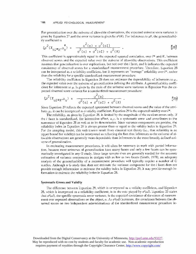
For generalization over the universe of allowable observations, the expected universe score variance isgiven by Equation 27 and the error variance is given by a2(R). For inferences to ~<*. the generalizabil-ity coefficient is

This coefficient is approximately equal to the expected squared correlation, over 1* and I2, betweenobserved scores and the expected value over the universe of allowable observations. This coefficientassumes that generalization is over replications, but not over the i facet, and it indicates the expectedconsistency of observed scores for a standardized measurement procedure. Therefore, Equation 28can be interpreted as a reliability coefficient, but it represents an &dquo;average&dquo; reliability over 1*, ratherthan the reliability for a specific standardized measurement procedure.

The reliability coefficient in Equation 28 does not estimate the dependability of inferences to 11,,,the expected value over the universe of generalization defining the attribute. A generalizability coeffi-cient for inferences to p~, is given by the ratio of the universe score variance in Equation 9 to the ex-pected observed score variance for a standardized measurement procedure:

Since Equation 29 reflects the expected agreement between observed scores and the value of the attri-bute, ¡.aeo, it can be interpreted as a validity coefficient. Equation 29 is the expected validity over 1*.

The reliability, as given by Equation 28, is limited by the magnitude of the random errors only. Ifthe facet is standardized, the interaction effect, ao,~, is a systematic error and contributes to thenumerator of Equation 28 as well as to its denominator. Since variance components are positive, thereliability index in Equation 28 is always greater than or equal to the validity index in Equation 29.For the sampling model, this well-known result from classical test theory (i.e., that reliability is anupper bound for validity) can be interpreted as reflecting the fact that inferences to the universe of al-lowable observations are generally more dependable than inferences to the more broadly defined uni-verse of generalization.

In evaluating measurement procedures, it will often be necessary to work with partial informa-tion, because most universes of generalization have many facets and only a few facets can be syste-matically investigated in any G study. Since large sample sizes are generally needed for the accurateestimation of variance components in designs with as few as two facets (Smith, 1978), an adequateanalysis of the generalizability of a measurement procedure will typically require a number of Gstudies. Although a G study that does not estimate the variance component for the i facet does notprovide enough information to estimate the validity index in Equation 29, it may provide enough in-formation to estimate the reliability index in Equation 28.

Systematic Errors and validity

The difference between Equation 29, which is interpreted as a validity coefficient, and Equation28, which is interpreted as a reliability coefficient, is in the role played by o~(o7). Equation 25 statesthat a2(~I), the specific systematic error variance, is the expected covariance of the errors of measure-ment over repeated observations on the object, o. As c~(o7) increases, the covariance between the ob-served scores on two independent administrations of the standardized measurement procedure in-



145

creases, and thus the reliability increases. However, as a2(ol) increases, the validity coefficient inEquation 29 decreases. By contrast, both the reliability and validity are decreasing functions of oz(~Z),the random error variance.

For a standardized measurement procedure, taking the expected value over repeated measure-ments implies taking an expected value over ~Z but not over I; and the expected value over the uni-verse of allowable observations, pt, is analogous to the &dquo;true&dquo; score of classical test theory. In the lim-it, as the number of replications approaches infinity, the magnitude of the random errors approacheszero, and the observed score approaches Vt. Therefore, pj is a parameter for which the standardizedmeasurement procedure provides unbiased estimates. Since the measurement procedure is intendedto provide estimates of the universe score, pi,,, the correlation between ii, and pt provides an index ofthe agreement between what the procedure actually estimates without bias and what it is intended toestimate. The expected value over I of the squared correlation between pt and IA,, is approximatelyequal to

Equation 30 is approximately equal to the squared correlation between the universe score and an ob-served score for which the sampling of the universe of allowable observations is sufficiently thoroughso that random errors can be ignored; in the limit, as 11,- approaches infinity, a2(IZ) approaches zeroand Equation 29 reduces to Equation 30. Since a2(R) cannot be negative, Equation 30 provides anupper bound on Equation 29 and therefore provides an upper bound on the validity of the

standardized measurement procedure.Equation 30 can be represented as a validity coefficient corrected for attenuation.

where the numerator of Equation 31 is the validity coefficient given by Equation 29 and the denomi-nator is the reliability coefficient given by Equation 28. ~~2(~;~; ~) represents a disattenuated validitycoefficient for the standardized measurement procedure.

The Reliability-Validity Paradox

The inference from the observed score to the universe score can be separated into two parts. Thefirst part is an inference from the observed score to pt~, the expected value over the universe of allow-able observations; and the second part is an inference from /1~ to /1°’ the expected value over the uni-verse of generalization, or the universe score. The dependability of inferences from observed scores touniverse scores can be factored to reflect these two partial inferences:

The first factor in Equation 32 is a reliability coefficient and represents the dependability of infer-ences from observed scores to p~-. The second factor in Equation 32 is a disattenuated validity coeffi-cient and represents the dependability of inferences from pj to ~o.

It is clear from Equation 28 that the reliability, which is the first factor in Equation 32, is im-

proved by increasing the impact of the oI interaction variance. This can be accomplished by selecting



146

a single condition for standardization on the z facet. Since the ol interaction is the specific systematicerror, this approach to improving reliability has an undesirable consequence; as can be seen fromEquation 30, it decreases the disattenuated validity coefficient, which is the second factor in Equation32 and thereby decreases the overall validity. Therefore, attempts to increase reliability by standard-ization of the measurement procedure may decrease validity (Lord & Novick, 1968, p. 334).

Convergent Validity

The sampling model analyzes reliability and validity in terms of the evidence for inferences fromobserved scores. In its emphasis on the justification of inferences, or interpretations, the samplingmodel is akin to the more general view of validity embodied in construct validity (Cronbach & Meehl,1955), which is discussed in a later section. At this point, it is convenient to discuss one form of con-struct validity, namely, convergent validity (Campbell & Fiske, 1959), in terms of the sampling model.

Convergent validity is generally evaluated in terms of the correlations between measurements ofan attribute obtained by several different methods. If these correlations are low, the observed scoresare seen as being contaminated by method variance, and the validity of any of the methods for mea-suring the attribute must be doubted. If the correlations are higher, convergent validity is supported.The logic of convergent validity requires that several different methods be available for the measure-ment of an attribute and therefore assumes that the attribute is a general property not tied to a partic-ular method of observation.

The convergent validity of a measurement procedure can be examined by letting the i facet repre-sent different methods of observation (e.g., objective tests, ratings, observation procedures). A mea-surement procedure employing a particular method is standardized to that condition of the methodfacet. With 1* representing a standardized method, the reliability of a measurement procedure canbe represented by Equation 28, and its validity can be represented by Equation 29. The validity coeffi-cient in Equation 29 is approximately equal to the expected correlation between scores based on dif-ferent methods (Kane & Brennan, 1977), and therefore it provides an index of the average &dquo;conver-gent validity&dquo; over pairs of methods.

Convergent validity (Campbell & Fiske, 1959) has generally been analyzed in terms of the correla-tions between specific pairs of methods, rather than the average correlation given by an intraclass cor-relation coefficient like Equation 29. Boruch and Wolins (1970) have advocated the use of ANOVA topartition observed score variance into components for traits, method, and random error; however,Schmitt, Coyle9 and Saari (1977) have criticized the use of the analysis of variance in evaluating con-vergent validity because it does not provide information about the convergent validity for particularmethods. The choice of a specific methodology is not crucial for the sampling model. Although thispaper has used analysis-of-variance models to develop the sampling model, correlational methodswould be more appropriate whenever the properties of specific methods were of interest.

Convergent validity is basically invariance over methods and depends on the interpretation of theattribute as a general property that is not linked to a specific method of observation. Assuming that Irepresents a method, the systematic errors ~ol are the object-method interactions. For a particularmethod I*, ~o,~ represents the specific systematic error that results from using method 1*. A largevalue for o2(0~ means that method has a serious effect on the results of measurement, and thereforegeneralization over methods is not appropriate.

The definition of an attribute implies invariance over all facets in the universe of generalization,including those that are standardized. If all of the invariance properties were tested and verified, thenthe measurement procedure would be valid. If some of the invariance properties were tested and no



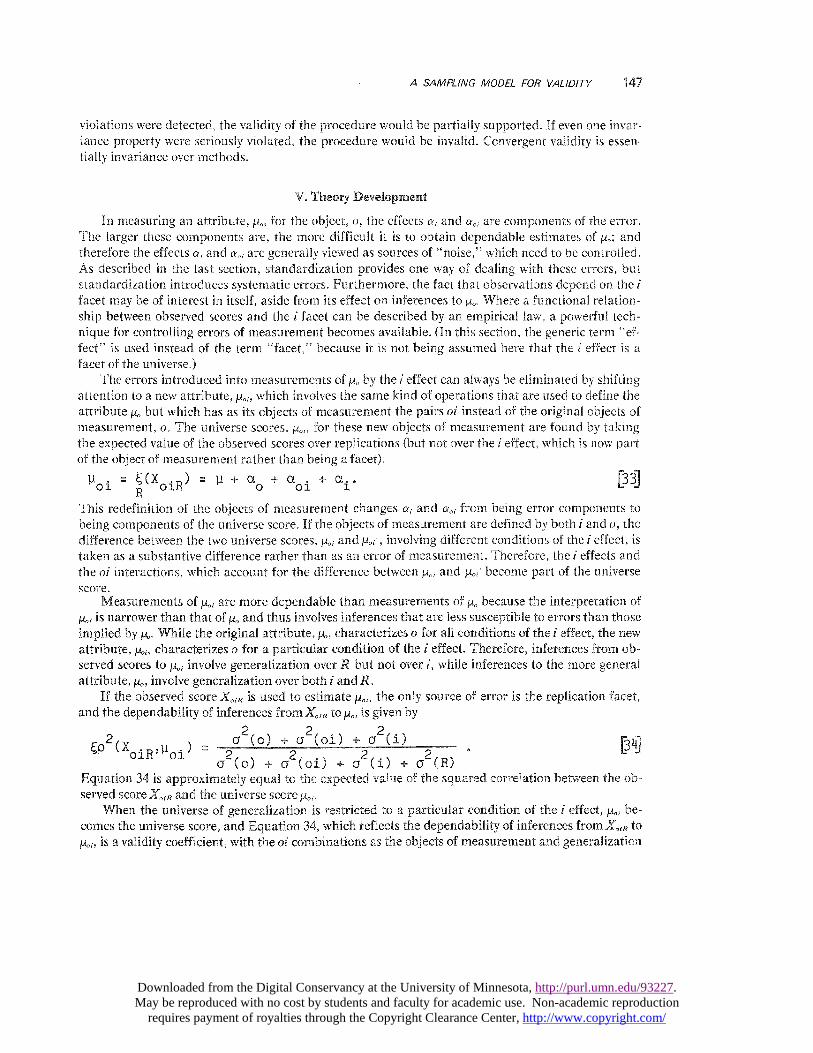
147

violations were detected, the validity of the procedure would be partially supported. If even one invar-iance property were seriously violated, the procedure would be invalid. Convergent validity is essen-tially invariance over methods.

V. Theory Development

In measuring an attribute, ~~, for the object, o, the effects a; and ai are components of the error.The larger these components are, the more difficult it is to obtain dependable estimates of ~n; andtherefore the effects a; and ~o; are generally viewed as sources of &dquo;noise,&dquo; which need to be controlled.As described in the last section, standardization provides one way of dealing with these errors, butstandardization introduces systematic errors. Furthermore, the fact that observations depend on the ifacet may be of interest in itself, aside from its effect on inferences to 1A.. Where a functional relation-ship between observed scores and the i facet can be described by an empirical law, a powerful tech-nique for controlling errors of measurement becomes available. (In this section, the generic term &dquo;ef-

fect&dquo; is used instead of the term &dquo;facet,&dquo; because it is not being assumed here that the i effect is afacet of the universe.)

The errors introduced into measurements of p. by the i effect can always be eliminated by shiftingattention to a new attribute, ~o;, which involves the same kind of operations that are used to define theattribute p~o but which has as its objects of measurement the pairs ®i instead of the original objects ofmeasurement, o. The universe scores, /loi’ for these new objects of measurement are found by takingthe expected value of the observed scores over replications (but not over the i effect, which is now partof the object of measurement rather than being a facet):

This redefinition of the objects of measurement changes cr~ and c~a; from being error components tobeing components of the universe score. If the ®byects ®f measurement are defined by both i and ®9 thedifference between the two universe scores, p~; and p~o;’, involving different conditions of the i effect, istaken as a substantive difference rather than as an error of measurement. Therefore, the i effects andthe ®i interactions, which account for the difference between JAoi and ~oz’ become part of the universescore.

Measurements of p., are more dependable than measurements of V,, because the interpretation of~o; is narrower than that of ii, and thus involves inferences that are less susceptible to errors than thoseimplied by 00. While the original attribute, /-10, characterizes o for all conditions of the effect, the newattribute, ~~, characterizes o for a particular condition of the effect. Therefore, inferences from ob-served scores to tAi involve generalization over R but not over i, while inferences to the more generalattribute, JAo, involve generalization over both i andR.

If the observed score XoiR is used to estimate JAoi’ the only source of error is the replication facet,and the dependability of inferences from XoiR to ~o; is given by

Equation 34 is approximately equal to the expected value of the squared correlation between the ob-served score XoLR and the universe score ~.

When the universe of generalization is restricted to a particular condition of the effect, /Áoi be-comes the universe score, and Equation 34, which reflects the dependability of inferences from Xo~R to~oi9 is a validity coefficient, with the ~a~ combinations as the objects of measurement and generalization



148

over l~. This validity coefficient 4Q2(X,i&dquo; IA,,i) is never less than the validity coefficient ~~Z(X~,~,t9 ~) withobjects of measurement, o, and generalization over i and R. Restricting the universe of generalizationiniproves the validity of measurement whenever 02(oi) or its greater than zero. (Under the sameconditions, standardization of the i facet improves reliability but does not necessarily improvevalidity.)

The increase in validity obtained by restricting the universe of generalization is part of a trade-offby which errors of measurement are reduced but the interpretation of the attribute is narrowed. Ahigh value for Equation 34 indicates that an inference from the observed score ~,~ to the universescore l.Aoi is dependable and therefore provides justification for such inferences. However, if Equation34 is to be a validity coefficient, inferences must be limited to the universe score p,,i for a specific valueof i. The value of Equation 34 does not indicate the dependability of inferences from ~~; to p,,; , theuniverse score for the same value of o and a different value of i, or to p~~9 the expected value of IA,,i overall values of i. Therefore, a high value for 4Q’(Xi,, fi~;) provides support for a relatively limited set ofinferences.

The expected squared correlation between the universe score IAi and the universe score IA. is ap-proximately equal to

Equation 35 can be derived by substituting &dquo;I&dquo; for ‘6I99 in Equation 14 and setting ~2(1~) equal to zero.That is, Equation 35 provides an index of dependability of inferences to bi. for observed scores basedon a single condition of the facet and an infinite number of replications. Furthermore, by comparingEquations 14, 34, and 35, it is clear that

&dquo; -. ~ ~ &dquo;&dquo;&dquo;&dquo;

Equation 36 partitions the dependability of inferences from ~;R to W,, into two parts. The first part,~~2(K~1~, f~~,.), represents the dependability of inferences from to ~~~, the expected value over repli-cations for a particular value of a. The second part, ~~Z(~o19~)9 is the dependability of inferences from~~; to P.. For the investigator who intends to generalize to the universe score, li., therefore, there is nobenefit in fixing the condition of the effect. As a matter of fact, the dependability of inferences to IA,would be improved by explicitly recognizing the i effect as a facet and by sampling it more

thoroughly.The main benefit derived from restricting the universe of generalization is the increase in validity

or the dependability of inferences from observed scores to universe scores. The main disadvantage inrestricting the universe of generalization is that it can lead to a large increase in the number of objectsof measurement in the population. If there were No objects in the original population and N condi-tions of the i effect, there are No N objects in the new population.

The choice between the more narrowly defined attribute, Vi, and the more broadly defined attri-bute, pu, must be made on pragmatic grounds; as Kaplan (1964, p. 77) has put it, &dquo;it is easy to

sharpen concepts as much as we like9 wh~t is hard is to determine whether this sharpness is worthachieving in a particular way.&dquo; For example, in analyzing data for a group of persons on several formsof a test, the investigator doing a generalizability study would often assume that the test forms aresampled from a universe of test forms and would generalize over test forms to IA.. However, the investi-gator could generalize to the universe scores ~01 for specific test forms, i, and thereby treat the scoreson the different test forms as separate variables. Covariance structure analysis (J6reskog, 1978; Linn



149

& Werts, 1979) provides one way to analyze the relationships among the different test forms. Covari-ance structure analysis seeks to estimate the reliability of particular measures by analyzing the vari-ances and covariances for these measures in terms of a specific model for the structure of the mea-sures.

In general, the investigator who views the attribute broadly enough so that the different condi-tions of the effect are associated with the same attribute will generalize to ~&dquo; while the investigatorwho is interested in the relationship among scores for specific conditions of the 1 effect will generalizeto p,,,, for the different test forms.

Inferences That Go the Model

In some cases, it is possible to characterize how 00i depends on i and c~ by developing an empiricallaw of the form:

where,f represents some function, v. is a variable that depends on o but does not depend on i, and WI isa variable that depends on i but not on o. An important special case of Equation 37 has the followingform:

where represents some function, and i* is a particular condition of the i facet. A new variable, 001*’ isdefined in terms of a specific reference condition, i*, for the i effect. This new variable can be substi-tuted for vo because it is a function of o but not of i. The fact that measurements of 001 and of y,;v aremore dependable than measurements of 00 facilitates the development of laws of the form given byEquation 38.

If a law like that in Equation 38 can be developed, the limitation inherent in measurements of p4,ican be overcome. With the help of Equation 38, information about pi.i* for any object provides infor-mation about 001 for all conditions of the effect for which w, is known. Inferences from observations

involving one condition of the i effect to what would be expected for another condition of the i effectare more difficult to develop than inferences based on invariance laws, but this more complicated ap-proach provides a more detailed analysis of the relationship between o and i.

The law of thermal expansion, relating length to temperature provides a good example of thekind of law indicated by Equation 38. Since variations in temperature generate errors in measure-ments of length, the accuracy of measurement can be improved by defining a new quantity, /,,~ as thelength of a bar, b, at temperature t. The object of measurement for lbt is a bar-temperature combina-tion, ht, instead of a bar. The attribute lb’ has a smaller universe of generalization than the attributeli,, and the direct interpretation of measurements of /,, are restricted to the temperature t. However,this restriction is effectively eliminated by the law of thermal expansion, which can be written as

where t* is some fixed reference temperature. (For convenience, t* is often taken to be 20’C, a com-fortable value for room temperature.) For a fairly wide range of temperature, the coefficient ofthermal expansion, k, is a constant. Because temperature variations introduce error into measure-ments of /,, lht~ can be measured more dependably than h. Since temperatures can be measured veryaccurately, and since Equation 39 provides a good fit to data over a wide range of temperatures, fix-ing the temperature for measurements of length does not seriously limit the interpretation of thesemeasurements.



150

Examples of the model in Equation 37 are provided by latent trait theories (Lord, 1980; ~right ~Stone, 1979), which represent the probability that a person answers an item correctly in terms of theability of the person and one or more item parameters. The ability parameter is an attribute of theperson and is assumed to depend on the person but not on the sample of items used to estimate it.The item parameters are attributes of items and are assumed to depend on the items but not on thesample of persons used to estimate them. Once the ability and item parameters for the latent traitnzodel are estimated, an equation like Equation 37 can be used to estimate the performance of eachperson to each item.

Note that an invariance property is a special case of Equation 38. In particular, if the function, ~,is such that ~,; is a constant for all valnes of i, JAoi is invariant with respect to the i facet. In such cases,there is no loss involved in taking o, instead of oi, as the object of measurement and there is some gainin simplicity. (In practice, it is often convenient to assume that p,i is invariant with respect to the i fa-cet, even where this assumption is known not to hold exactly.)

The Biidge A~~I®~The observations involved in measurement are of interest mainly because they support inferences.

These inferences are of two kinds. First, there is an inference from the observation to the universescore. Second, there are inferences from one universe score to other universe scores and to other ob-servations. Using the bridge analogy of Cornfield and Tukey (1956, p. 912), these two inferences canbe viewed as two spans of a bridge crossing a river. The first span represents inferences from the ob-served score to a universe score, and the second span represents inferences from the universe score tothe universe scores for other attributes. If the second span is firmly supported by empirical laws, itmay be made quite long without weakening the total inference, thus making it profitable to shortenthe first span by narrowing the universe of generalization.

Inferences from observed scores to the universe score JAoi for the restricted universe of generaliza-tion have a higher validity than inferences to /10. Therefore, restricting the universe strengthens thefirst span. A well-confirmed law of the type given in Equation 38 provides a strong second span byjustifying inferences from one universe score to another. In such cases, restricting the universe of gen-eralization does not limit the generality of the inferences; the second span is simply bearing more re-sponsibility for the total inferences.

The of Measurements

In discussing inferences that go beyond the universe of generalization, it is useful to define a thirdproperty of measurement in addition to reliability and validity, This third property, the import ofmeasurement, is associated with the total significance of what can be inferred from the measurement.Hempel (1952) introduced import in terms of an example: i

... we might define the hage of a person as the product of his height in millimeters .and his agein years. This definition is operationally adequate and the term &dquo;hage&dquo; thus introduced wouldhave relatively high precision and uniformity of usage; but it lacks theoretical import, for wehave no general laws connecting the hage of a person with other characteristics. (p. 46)

Import is a qualitative concept, which emphasizes the scope and significance of the inferences thatcan be drawn from a measurement.

The invariance laws that justify the interpretation of observations as measurements provide a coreof import to all measurements. These laws support inferences from the observed scores to the universe



151

score and, also, to all other observed scores in the universe of generalization. If the attribute is not in-volved in any other empirical laws, the invariance laws define the total import of the measurement.The extent to which the invariance laws lend import to measurements depends in part on the general-ity of these laws. If attention is restricted to the invariance properties implied by their definitions, theattribute 1A,, has greater import than the attribute ~o;. As such, measurements of ¡.aeoi do not justify infer-ences to other conditions of the i facet. Measurement of /10, on the other hand, involves generalizationover all conditions of the i facet.

In practice, the development of empirical laws can lead to simultaneous increases in both thevalidity and the import of measurements. This is accomplished by partitioning the universe of gener-alization into a number of more narrowly defined subuniverses, while connecting the universe scoresfor these subuniverses through empirical laws. Physics has used this strategy very effectively. Mea-surement of such basic attributes as length have been gradually refined by restricting various facets intheir universe of generalization. At the same time, the import of length measurements has been in-creased by theories like Euclidian geometry and classical mechanics.

The of Theories

Attributes that play a central role in fundamental theories have greater import than attributeswhich are involved in one or two isolated empirical l~ws, or in no laws at all. The empirical laws thatdetermine the content of a theory and provide confirmation for the theory add to the import of all ofthe attributes involved in the theory. Theories extend the range of inferences that may be drawn frommeasurements and therefore increase their import. However, according to the sampling model, thevalidation of measurements that are interpreted as dispositions does not depend on theory.

Measurements of a disposition are valid to the extent that they provide accurate estimates of uni-verse scores. The existence of laws or theories involving a dispositional attribute has no direct bearingon the validity of measurements of the attribute. For example, within atomic theory, the law ofthermal expansion, Equation 39, can be at least partially explained in terms of the motion ofmolecules. However, the theory is not necessary in order to interpret the coefficient of thermal expan-sion, k, which is simply the rate at which length changes as a function of temperature. The theory pro-vides a causal explanation of thermal expansion but is not needed for the interpretation of k as a dis-positional attribute and is therefore not used in validating measurements of k.

This point of view is generally consistent with the interpretation of measurements in science. Inhis analysis of measurement in physics, Campbell ~I921, p. 134) concluded that &dquo;measurement is es-sential to the discovery of laws&dquo; but he did not use the laws to evaluate measurement procedures.Similarly, Suppes and Zinnes (1963) and, more recently, Krantz, Luce, Suppes, and Tversky(1971)did not find it necessary to consider most of the laws involving attributes in their detailed analyses ofmeasurement.

Although they do not have a direct role in validating measurements for dispositional attributes,theories have a significant indirect influence on the validity of such measurements. They make itfeasible to restrict the universe of generalization for attributes are therefore to increase the validity ofmeasurements without decreasing their import. These more narrowly defined attributes depend onthe theories for much of their import, while the magnitude of the errors of measurement are reducedbecause fewer invariance properties are required.

The ‘~&dquo;~~d~®ff Between and t

If import is ignored, it is easy to generate measurements with a high degree of validity by definingthe universe of generalization narrowly enough so that the inferences to the universe scores involve



152

generalization over few facets. Such inferences are likely to be very dependable. In the limiting case,where observations are interpreted simply as observations, there is no inference and, therefore, nochance of an invalid inference.

However, the issue of import cannot be ignored, and trade-offs between validity and import mustbe made; Kaplan’s (1964, p. 77) question about the appropriate degree of sharpness for conceptsmust be addressed. The researcher who interprets observations narrowly draws more accurate infer-ences but also says less about the world than the researcher who interprets observations broadly. Thechoice between narrow but dependable interpretations and broader, but less dependable, interpreta-tions is a choice of strategy. The continuum of available options has strict operationalism at one endand construct validity at the other end.

Strict operationalism tries to define attributes narrowly enough to insure that the validity of theinterpretations is essentially perfect (Bechtoldt, 1959). The strict operationalist is unwilling to giveany hostages to the future in the form of assumed invariance properties that might turn out to be onlyapproximations. Strict operationalism is the strategy of pure empiricism, and theory plays essentiallyno role. As described by Cronbach and ~eehl (1955), construct validity defines an attribute in termsof all of the relationships in which it appears. From the standpoint of construct validity, the definitionof an attribute entails various laws; and in order for a measurement procedure to be valid, all of theselaws must be satisfied.

Constmct Validity

According to the American Psychological Association Standards (American Psychological Associ-ation, 1974), a psychological construct is &dquo;a theoretical idea developed to explain and to organizesome aspects of existing knowledge,&dquo; and construct validity occurs &dquo;when one evaluates a test orother set of operations in light of the specified construct&dquo; (p. 29). Cronbach and Meehl (1954) sum-marized the logic of construct validity by saying,

Construct validation takes place when an investigator believes that his [or her] instrument re-flects a particular construct, to which are attached certain meanings. The proposed interpreta-tion generates specific testable hypotheses, which are a means of confirming or disconfirmingthe claim. (p. 255)

A dispositional attribute is defined by its universe of generalization, and the laws involved in givingmeaning to such constructs are the invariance properties. The sampling model assumes that the inter-pretation of a measurement generates testable hypotheses-the invariance properties, which can beused to test the validity of the interpretation.

The sampling model is generally consistent with construct validity. Like construct validity, it sug-gests that validity is more accurately represented as a series of upper bounds than as a single number.Since most attributes assume invariance over a number of facets, it will usually require a series ofstudies to establish invariance over all of the potentially important facets. If one or more of the re-quired invariance properties does not hold, there are two general options available (see Cronbach &

Meehl, 1955, p. 260-264). First, the measurement procedure can be modified, possibly by samplingmore thoroughly or by standardizing some facets. Second, the attribute’s definition can be changedby restricting the universe of generalization.

Although the sampling model is consistent with construct validity in most ways, it is less generalin the interpretations to which it can be applied. The sampling model emphasizes the interpretationof attributes as dispositions, which are defined in terms of universes of observations, while construct



153

validity applies to a variety of constructs ranging from theoretical attributes embedded in extensivenetworks to basic dispositions. Theoretical constructs derive their meaning from the axioms of atheory (Braithwaite, 1953) and are said to be defined implicitly by the network of laws implied by theaxioms of the theory. Measurements of an implicitly defined construct are validated by verifying thetheory. Because Cronbach and Meehl (1955) tend to emphasize the role of theory in providing an im-plicit definition for theoretical constructs, they suggest that all of the laws involving an attributeshould be used in validating measurements of the attribute.

Because construct validity may apply to any kind of interpretation, it is more general than thesampling model. However, the dispositional interpretations emphasized by the sampling model areparticularly important in science because they are especially relevant to the central activity of sci-ence-theory testing. In order to avoid circularity, the measurements that are used to test a theorymust not depend on the theory for their validity. Therefore, in testing theories, dispositional interpre-tations are typically emphasized in place of more theory-laden interpretations.

The observations used to measure a theoretical attribute can generally be interpreted on at leasttwo levels. First, the observations can be interpreted as samples from the universe of generalizationdefining a disposition. The sampling model suggests methods that are appropriate for evaluating thevalidity of a dispositional interpretation. Second, the observations can be interpreted as reflecting atheoretical construct which is implicitly defined by a theory. Although Cronbach (1980b) has sug-gested that a distinction be drawn between laws involved in the &dquo;core meaning&dquo; of a construct andother hypotheses that &dquo;we are ready to abar~d®~9&dquo; there are no general criteria for deciding which ofthe laws in which an attribute appears are most relevant to its construct validity.

Use of the F 1 ~e~®~k---~, ~~~ct~eal Consideration

In those cases where extensive theory exists, the effort required to test all of the implications ofthe theory is likely to be prohibitive for any investigator. And since theories in the behavioral sciencesare often rather loose, the evidence for validity derived from the theory is likely to be ambiguous atbest and inconsistent at worst. By assuming that the theory as a whole implicitly defines constructs,Cronbach and Meehl (1955) present an extremely formidable task to the investigator seeking to estab-lish construct validity, and it would be useful to establish priorities for which laws or theories shouldbe included in validity studies.

The sampling model’s distinction between validity and import provides a basis for setting priori-ties. Validity is defined in terms of invariance over a universe of generalization and is associated withthe &dquo;meaning&dquo; of an attribute in the narrow sense of denotation. Import is defined in terms of all ofthe relationships in which the attribute is involved and is associated with &dquo;meaning&dquo; in the broadersense of connotation. The sampling model emphasizes the interpretation of attributes as dispositionsand equates validation with the testing of invariance laws9 the theory as a whole defines the import ofmeasurements and therefore has a strong, but indirect, effect on validation.

By checking the invariance laws, the investigator establishes that the measurements support in-ferences of some generality and are not simply reports of isolated incidents. The invariance laws pro-vide the &dquo;core meaning,&dquo; or denotation, for basic attributes. The core meaning of derived attributesincludes their defining laws (e.g., the law of thermal expansion for the coefficient of thermal expan-sion) in addition to the invariance laws. The validation of theoretical attributes, which are implicitlydefined by a theory, involves the confirmation of the theory as a whole. However, even for the mosttheoretical of constructs, the sampling model suggests a reasonable place to begin the study ofvalidity.



154

a The of Sampling M eI~ for ValidityThe sampling model is basically quite simple. A dispositional attribute is defined in terms of a

universe of generalization. The &dquo;true&dquo; value of the attribute is the universe score, equal to the ex-pected value over the universe of generalization. Measurement involves inferences from observationsto the expected value over the universe defining an attribute, and a measurement procedure is valid tothe extent that its inferences about universe scores are accurate. For these inferences to be justified,certain invariance laws must hold, at least approximately, and these laws should be verifiedempirically.

Although the application of the model becomes more complicated when standardization andtheory development are considered, the basic premises remain quite simple. The sampling modelmakes no assumptions about underlying structures or processes; it neither affirms nor denies the ex-istence of such theoretical constructs. It makes no assumptions about the distribution of observedscores, the distribution of universe scores, or the relationships between different kinds of scores. Themodel does not dictate what kinds of conditions can be defined as facets. The only restriction put onthe universe of generalization is that it be sufficiently well defined that it is possible to test the invar-iance laws associated with the universe.

to the Sampling Model

A number of authors (Gillmore, 1979; Loevinger, 1965; Rozeboom, 1966) have objected tosampling models by pointing out that measurements do not generally consist of random samples froma clearly defined universe of generalization. Within the sampling model, the sequence of inferencesinvolved in going from observed scores to universe scores can be analyzed explicitly, thus making itunnecessary to assume that measurement involves random sampling from the universe of generaliza-tion. However, the model does require that universes be defined well enough to allow for the testing ofthe invariance laws.

Some progress has been made in developing more precise definitions for universes. For example,Anderson (1972), Bormuth (1970), and Popham (197~) have proposed methods for the specification ofthe item facet for achievement tests, and Fiske (1977) and Wiggins (1973) have discussed the defini-tions of a variety of facets. However, there is still considerable ambiguity in the universe definitionsfor scientific attributes. In discussing the semantics of natural languages, Clark and Clark (1977, p.412) have pointed out that &dquo;the boundaries for most categories are fuzzy. There is no clear boundarybetween trees and one category shades off into the other.&dquo; Similarly, Nagel (1971, p. 30) talksabout the &dquo;penumbra of vagueness&dquo; of all scientific terms. The sampling assumptions required forthe interpretation of measurement are typically not satisfied exactly; like all models, the samplingmodel is only an approximation.

In light of the substantial difficulties in drawing random samples from the universe of generaliza-tion, the verification of the invariance laws presents a serious problem. The invariance laws are gener-al empirical laws, and their testing involves inductive inferences similar to those involved in the test-ing of any empirical laws. In practice, a measurement procedure is evaluated in a series of studies inwhich its invariance laws are examined.

Invariance Laws and Inductive Inference

Even a cursory review of the issues involved in inductive inference would go far beyond the scopeof this paper, but some general remarks on this topic may put the problem of testing the invariance



155

laws into perspective. According to Popper (1965, 1968), laws are conjectures which are subject topossible refutation but not to confirmation. A general law applies to many observations, and any ofthese observations could be used to test the law. A deterministic law that fails a single test or a statisti-cal law that fails a large proportion of its tests is refuted. A law which is subjected to a wide variety ofempirical tests without being refuted is supported by these tests.

There is a clear lack of symmetry in Popper’s views; a law can be decisively refuted, but even alarge number of studies cannot definitely confirm the law. The more challenges of various kinds thata law has been exposed to without being refuted, the more strongly it is considered to be supported,but the law is never completely confirmed. In discussing validation, Cronbach (1980a) has made asimilar point:

The job of validation is not to support an interpretation, but to find out what might be wrongwith it. A proposition deserves some degree of trust only when it has survived serious attempts tofalsify it. (p. 103)

In a sense, Popper replaces the concept of confirmation by the concept of degree of confidence. A lawis subjected to empirical challenges, and confidence in the law increases whenever it meets a chal-lenge (Lakatos, 1970).

According to the sampling model, the definition of an attribute involves a universe of generaliza-tion. The claim that a measurement procedure generates valid measurements of the attribute is

equivalent to the conjecture that the observed scores are invariant with respect to sampling from thisuniverse. This conjecture can be decomposed into a number of specific invariance laws, each of whichapplies to a specific facet. A successful test of any one of the invariance laws, based on a randomsample of conditions from the facet, provides direct support for the specific invariance law and somesupport for the cluster of invariance laws associated with the attribute. As more and more invariance

properties are investigated without encountering refutations, the degree of confidence in the validityof the measurements increases.

The strength of the evidence for validity provided by invariance over a particular facet will dependon the facet studied. If there is some reason to suspect that the facet may have a large effect on ob-served scores, evidence for invariance over that facet answers a serious challenge and therefore pro-vides strong support. Note that G studies, which sample from only part of a facet, do not test invari--ance over the full facet. They do provide evidence for invariance over the subuniverse sampled. Be-cause they answer one possible challenge to the invariance law, they provide some evidence forvalidity, but they are not very effective in establishing the limits of the universe.

Since it is usually not possible to estimate variance components for more than a few facets withouthaving very large sample sizes, the validation of most measurement procedures will require a series ofstudies in which the invariance properties are systematically investigated. Those facets that are ex-pected to introduce the greatest error variance should be investigated first. Subsequently, other facetscan be investigated. The resulting sequence of upper bounds on validity is perhaps less satisfactorythan a point estimate of validity, but it is probably more realistic to consider any coefficient resultingfrom a G study as an upper bound than as an unbiased point estimate of validity.

The ~r~c ~~~ Effect in ~~ff~~~n~ ~Jn~~a~~~~~ of Generalization

Throughout most of this paper, it has been tacitly assumed that the conditions defining a facetare given and that the task is to check the appropriate invariance laws. For purposes of exposition,this assumption has been convenient, but in practice the situation is never quite this simple. Although



156

Popper (1965, 1968) has emphasized the testing of laws, the invariance requirement may also be ad-dressed by defining facets so that the observations are invariant over the facet.

Toulmin (1953) described scientific laws as rules of inference, rather than as inductive generaliza-tions. The question to be asked about such rules of inference is not whether or not they are true, buthow widely they apply. Toulmin’s analysis is quite different from Popper’s; but for the purposes ofthis paper, these two views are complementary. Toulmin’s (1953) treatment of scientific laws as rulesof inference fits the sampling model especially well. The whole purpose of the invariance properties is,in fact, to justify inferences from observed scores to universe scores.

As applied to the invariance la~s9 thc task of determining how widely the law applies is closelyconnected with the task of clarifying the boundaries of the universe of generalization. Toulmin makesthe point that the range of applicability of a law is generally not known when the law is first proposed,and one of the aims of ei-npirical research is to determine how widely the law applies. The aim ofempirical investigations of the invariance laws is to see how widely observed scores can be generalized.

In most cases, decisions about whether or not to generalize over a class of conditions will depend,in part, on whether observations are invariant over the conditions. If the observations are not invari-ant over a facet, including the facet in the universe of generalization would decrease the validity ofmeasurements of the attribute; therefore, the facet is not likely to be included in the definition of theuniverse. However, if the observations are invariant over the facet, including the facet in the universewould not decrease validity and would increase the usefulness of the measurements. The universe ofgeneralization is designed so that the invariance laws will hold. Lumsden (1976, p. 271) makes asimilar suggestion.

Random from the Universe of Aflowable 0bseiwationu

The purpose of G studies is to provide data that can be used in the design of effective measure-ment procedures. In particular, an important goal in designing a measurement procedure is to reducethe number of facets that must be randomly sampled in obtaining an observed score. There are threeways to do this. First, if G studies show that all of the variance components (for the main effect andinteractions) for a facet arc zero, there is no need to be concerned about how this facet is sampled.Second, facets that have been standardized are not sampled in estimating universe scores, althoughthe magnitude of the systematic errors for these facets must be estimated in G studies. Third, if theuniverse of generalization is restricted in connection with the development of theory, thus defining anew attribute, measurements of the new attribute will not involve sampling of the facet.

All of these modifications of the measurement procedure tend to decrease the number of facetsthat are randomly sampled for each observed score. The only facets that need to be sampled random-ly arc those for which interactions with the object of measurements are fairly large and apparentlyrandom. Efforts to obtain random samples can be concentrated on these faccts; and if the number ofsuch facets can be decreased, the difficulty in taking random samples from the universe of allowableobservations is reduced.

The Role of in the Universe of Generalization

The universe of generalization is, to a large extent, shaped by theory. This occurs in at least threeways. First, as discussed earlier, those effects that are explicitly involved in the theory are treated asfixed conditions in the universe of generalization rather than as facets.



157

Second, theory often suggests the kinds of observations that should be considered equivalent inthe sense of belonging to the same universe of generalization. For example, a cognitive psychologistmight put the responses to a certain question into the same universe of generalization, whether thequestion was written, spoken, or projected on a screen and whether the responses were made byspeaking, writing, pressing a button, or giving a hand signal. Since the observations in this universehave few surface features in common, it is the theoretical assumptions about cognitive processes thatsupplies impetus for putting them into the same universe of generalization. One advantage of design-ing attributes to fit a theory is that the import of the theory is built into the attribute.

Third, instead of defining an attribute in terms of the mean over the universe of generalization orin terms of a particular condition of a facet, it is often useful to define the attribute in terms of an&dquo;ideal&dquo; limiting condition which never occurs in practice. This avoids having the properties of themeasurements determined by any particular condition of observation. The interpretation of humanabilities in terms of the best performance, rather than typical performance, involves this kind of idealcondition. Since the best performance can occur only if the person has adequate time to finish thetask, abilities are associated with neither a fixed time limit nor with the mean over a time-limit facet.The assumption that the time limit does not affect performance substantially could be investigated byconducting an experiment in which the time limit is extended; if performance improves significantly,the time limit is too short.

The Steady State Requirement

Cronbach et al. (1972, p. 364) have stated that because generalizability theory &dquo;treats conditionswithin a facet as unordered it will not deal adequately with the stability of scores that are subject totrends , , ,&dquo; and that &dquo;the concept of universe score is of dubious value if the universe stretches over aperiod when the person’s status is changing regularly and appreciably.&dquo; According to the samplingmodel, to generalize over a facet is to treat the variability of observed scores due to the sampling of thefacet as error. If conditions of some kind are considered a facet, the attribute is the expected valueover all conditions of the facet and is not associated with any particular condition. For a relationshipto exist between observed scores and the conditions of a facet, each observed score must be associatedwith a particular condition of the facet, and this is not consistent with the interpretation of the facetas a source of error. Therefore, an effect cannot be interpreted as a facet and at the same time as anattribute to be systematically investigated.

The problems associated with trends can be eliminated as soon as the trend is detected; this is ac-complished by restricting the universe of generalization for each observation to a fixed condition ofthe facet involved and by treating the trend as an empirical law. Undetected trends will tend to causethe variance components for the facet to be large, and therefore the examination of variance compo-nents can facilitate the detection of trends.

The Analysis-of-Variance as a Tool

Although the analysis of variance is a useful tool for the sampling gnodel, the formal statisticalmodels defining variance components should not be allowed to obscure the fundamental concernsembodied in the invariance properties. As Cronbach (1976) has observed, the technical apparatus ofgeneralizability theory is less important than the questions suggested by the theory. The samplingmodel provides a framework for considering the issues that arise naturally in the interpretation of



158

measurements, The three types of issues that have been identified are those associated with reliability,validity, and import. For convenience, most of the discussion of these issues has been in terms of vari-ance components, but the same points could have been made using other terminology. In fact, wherethere is interest in the relationship among the observed scores for particular conditions of a facet, cor-relation coefficients might be preferred.

In some cases, it may be necessary to employ controlled experiments in investigating the effects ofa facet. For example, if an attribute is assumed to be unaffected by short periods of &dquo;coaching,&dquo; as isoften the case for aptitudes, it might be necessary to conduct controlled studies to check this assump-tion and to analyze the resulting data in a way that is consistent with the design of the study. Thesampling model requires that the invariance properties implicit in the definition of an attribute be in-vestigated; it does not specify how these invariance properties should be investigated.

Concluding Co1nnlentu

A dispositional attribute is defined in terms of a universe of generalization, and the universe scorefor the attribute is the expected value over this universe. Therefore, the universe score is a parameterdefined over the universe of generalization, rather than a hypothetical entity. Although the samplingmodel is basically quite simple, its application can be very difficult for two reasons. First, most mea-surement procedures are not designed in terms of random sampling from the universe of generaliza-tion, and therefore inferences from observed scores to the universe scores may be quite complicated.

The second and more fundamental difficulty is encountered in defining the universe of general-ization. As noted earlier, some progress has been made in the methodology for defining universes, butit is still true that the universes associated with most attributes are quite fuzzy. The difficulties in-volved in defining universes, and subsequently sampling from these universes, arise for measurementprocedures in all of the sciences. Violations of sampling assumptions introduce vagueness into whatwould otherwise be a precise statistical model, but they do not preclude effective use of the samplingmodel. Rather, the sampling model highlights the weakness of some inferences that are routinelymade in interpreting measurements and should therefore encourage research aimed at defining uni-verses more precisely.

Although the sampling model makes few assumptions, it provides an analysis of many issues as-sociated with the dependability of measurement. The sampling model makes it possible to givevalidity a straightforward interpretation and to draw a clear distinction between reliability andvalidity The model provides the basis for a detailed analysis of standardization and of the resultingsystematic errors. The conclusions that reliability is an upper bound on validity and that some meansof improving reliability may cause validity to decrease are easily derived from the model. Further-more, the model suggests an explicit mechanism for relating the refinement of measurement proce-dures to the development of laws and theories.

References

American Psychological Association. Standards foreducational and psychological tests. WashingtonDC: Author, 1974.

Anderson, R. C. How to construct achievement teststo assess comprehension. Review of Education Re-search, 1972, 42. 145-170.

Bechtoldt, M. P. Construct validity: A critique.American Psychologist, 1959, 14, 619-629.

Bormuth, J. K. On the theory of achievement testitems. Chicago: University of Chicago Press, 1970.

Boruch, R. F., & Wolins, L. A procedure for estima-tion of trait, method, and error variance attribut-able to a measure. Educational and PsychologicalMeasurement, 1970, 30, 547-574.

Braithwaite, R. B. Scientific explanation. Cambridge,England: Cambridge University Press, 1953.



159

Brennan, R. L. Generalizability analysis: Principlesand procedures (ACT Technical Bulletin No. 26).Iowa City IA: American College Testing Program,1977.

Brennan, R. L. Elements of generalizability theory(ACT Monograph 16). Iowa City IA: AmericanCollege Testing Program, in press.

Bridgman, P. W. The logic of modern physics. NewYork: Macmillan, 1927.

Campbell, D. T., & Fiske, D. W. Convergent and dis-criminant validation by the multitrait-multi-method matrix. Psychological Bulletin, 1959, 56,81-105.

Campbell, N. R. What is science? London: Methuen,1921.

Campbell, N. R. Foundations of science. New York:Dover Publications, 1957. (Originally published asPhysics: The elements. Cambridge, England:Cambridge University Press, 1920)

Cardinet, J., Tourneur, Y., & Allal, L. The symmetryof generalizability theory: Applications to educa-tional measurement. Journal of Educational Mea -surement, 1976, 13, 119-134.

Carnap, R. Testability and meaning. In H. Feigl &M. Brodbeck (Eds.), Readings in the philosophy ofscience. New York: Appleton-Century-Crofts,1953.

Carnap, R. The philosophy of science (M. Gardner,Ed.). New York: Basic Books, 1966.

Clark, H. H., & Clark, E. V. Psychology and langu-age. New York: Harcourt Brace Jovanovich, 1977.

Corben, H., & Stehl, P. Classical mechanics (2nd ed.).New York: John Wiley & Sons, 1960.

Cornfield, J., & Tukey, J. W. Average values of meansquares in factorials. Annals of Mathematical Sta-tistics, 1956, 27, 907-949.

Cronbach, L. J. Test validation. In R. L. Thorndike(Ed.), Educational measurement (2nd ed.). Wash-ington DC: American Council on Education,1971.

Cronbach, L. J. On the design of educational mea-sures. In D. N. M. de Gruijter & L. J. T. van der

Kamp (Eds.), Advances in psychological and edu-cational measurement. New York: John Wiley &Sons, 1976.

Cronbach, L. J. Validity on parole: How can we gostraight? New Directions for Testing and Mea-surement, 1980, 5, 99-108. (a)

Cronbach, L. J. Discussion. In Proceedings of confer-ence on construct validity in psychological mea-surement. Princeton NJ: Educational TestingService, 1980. (b)

Cronbach, L. J., & Gleser, G. C. The signal/noise ra-tio in the comparison of reliability coefficients.

Educational and Psychological Measurement,1964, 24, 467-480.

Cronbach, L. J., Gleser, G. C., Nanda, H., &

Rajaratnam, N. The dependability of behavioralmeasurements: Theory of generalizability forscores and profiles. New York: Wiley, 1972.

Cronbach, L. J., & Meehl, P. E. Construct validity inpsychological tests. Psychological Bulletin, 1955,52, 281-302.

Ebel, R. Must all tests be valid? American

Psychologist, 1961, 16, 640-647.Ebel, R. L. Explorations in reliability theory. Con-

temporary Psychology, 1974, 19, 81-83.Ellis, B. Basic concepts of measurement. Cambridge,

England: Cambridge University Press, 1968.Ennis, R. H. Operational definitions. In H. S.

Broudy, R. H. Ennis, & L. I. Krimerman (Eds.),Philosophy of educational research. New York:John Wiley & Sons, 1973.

Fiske, D. W. Measuring the concepts of personality.Chicago: Aldine, 1971.

Frank, P. Philosophical interpretations and misinter-pretations of the theory of relativity. In H. Feigl &M. Brodbeck (Eds.), Readings in the philosophy ofscience. New York: Appleton-Century-Crofts,1953.

Gillmore, G. M. An introduction to generalizabilitytheory as a contributor to evaluation research

(EAC Report No. 79-14). Seattle: University ofWashington, Educational Assessment Center,1979.

Hempel, C. G. Fundamentals of concept formation inempirical science. Chicago: The University of Chi-cago Press, 1952.

Hempel, C. G. Operationism, observation, andtheoretical terms. In A. Danto & S. Morgenbesser(Eds.), Philosophy of science. New York: NewAmerican Library, 1960.

Hempel, C. G. Aspects of scientific explanation andother essays in the philosophy of science. GlencoeIL: Free Press, 1965.

Jöreskog, K. G. Structural analysis of covariance andcorrelation matrices. Psychometrika, 1978, 43,443-477.

Kaiser, H. J., & Michael, W. B. Domain validity andgeneralizability. Educational and PsychologicalMeasurement, 1975, 35, 31-35.

Kane, M. T., & Brennan, R. L. The generalizabilityof class means. Review of Educational Research,1977, 47, 267-292.

Kaplan, A. The conduct of inquiry. San Francisco:Chandler, 1964.

Krantz, D., Luce, R. D., Suppes, P., & Tversky, A.Foundations of measurement (Vol. 1). New York:Academic Press, 1971.



160

Kuhn, T. S. The structure of scientific revolutions(2nd ed.). Chicago: University of Chicago Press,1970.

Lakatos, I. Falsification and the methodology of sci-entific research programs. In I. Lakatos & A.

Musgrave (Eds.), Criticism and the growth ofknowledge. London: Cambridge University Press,1970.

Lindquist, E. F. Design and analysis of experimentsin psychology and education. Boston: HoughtonMifflin, 1953.

Linn, R., & Werts, C. Covariance structures and theiranalysis. New Directions for Testing and Measure-ment, 1979, 4, 53-73.

Loevinger, L. Person and population as psychometricconcepts. Psychological Review, 1965, 72,143-155.

Lord, F. M. Applications of item response theory topractical testing problems. Hillsdale NJ: Erlbaum,1980.

Lord, F. M., & Novick, M. R. Statistical theories ofmental test scores. Reading MA: Addison-Wesley,1968.

Lumsden, J. Test theory. Annual Review ofPsychology. 1976, 27, 254-280.

McDonald, R. P. Generalizability in factorable do-mains : "Domain validity and generalizability."Educational and Psychological Measurement.1978, 38, 75-79.

Meehl, P. E. On the circularity of the law of effect.Psychological Bulletin, 1950, 47, 52-75.

Nagel, E. Theory and observation. In E. Nagel, S.

Bromberger, & A. Gumbaum, Observation andtheory in science. Baltimore : The Johns HopkinsPress, 1971.

Nunnally, J. C. Psychometric theory. New York: Mc-Graw Hill, 1967.

Physical Science Study Committee. College physics(U. Haber-Schain, Ed.). Boston: Heath, 1968.

Popham, W. J. Criterion-referenced measurement.Englewood Cliffs NJ: Prentice-Hall, 1978.

Popper, K. R. Conjecture and refutation: The growthof scientific knowledge. New York: Harper &Row, 1965.

Popper, K. R. The logic of scientific discovery. NewYork: Harper & Row, 1968.

Rozeboom, W. W. Foundations of the theory ofprediction. Homewood IL: Dorsey Press, 1966.

Schmitt, N., Coyle, B. W., & Saari, B. B. A reviewand critique of analyses of multitrait-multimethodmatrices. Multivariate Behavioral Research, 1977,12, 447-478.

Smith, P. L. Sampling errors of variance componentsin small sample multifacet generalizabilitystudies. Journal of Educational Statistics, 1978, 3,319-346.

Stallings, W. M., & Gillmore, G. M. A note on "ac-curacy" and "precision." Journal of EducationalMeasurement, 1971 , 8, 127-129.

Suppes, P. The structure of theories and the analysisof data. In W. F. Suppe (Ed.), The structure of sci-entific theories. Urbana IL: The University of Il-linois Press, 1974.

Suppes, P., & Zinnes, J. L. Basic measurement

theory. In R. D. Luce, R. R. Bush, & E. Galanter(Eds.), Handbook of mathematical psychology(Vol. 1). New York: John Wiley & Sons, 1963.

Toulmin, S. The philosophy of science. London:Hutchinson’s Universal Library, 1953.

Tryon, R. C. Reliability and behavior domain

validity; reformulation and historical critique.Psychological Bulletin, 1957, 54, 229-249.

Wiggins, J. S. Personality and prediction: Principlesof personality assessment. Reading MA: Addison-Wesley, 1973.

Winer, D. J. Statistical principles in experimental de-sign (2nd ed.). New York: McGraw-Hill, 1971.

Wright, B. D., & Stone, M. H. Best test design.Chicago: Mesa Press, 1979.

Authors Address

Send requests for reprints or further information toMichael T. Kane, American College Testing Pro-gram, P.O. Box 168, Iowa City IA 52243.



a sampling model for validity

Documents