a runge-kutta method for solving second order odes directly papers/pert vol. 10 (2) aug....

Pertanika 10(2), 209-217 (1987)

A Runge-Kutta Method for Solving Second Order ODEs Directly

MOHAMED B. SULEIMAN, JALIL ABD. GHANI and MOHRI B. IDRISMathematics Department,

Faculty of Science and Environmental Studies,Universiti Pertanian Malaysia,

43400 Serdang, Selangor, Malaysia.

Key words: Second order ordinary differential equations (ODEs); Runge-Kutta method; lineardifferential operator; extrapolated; tolerances.

ABSTRAK

Satu kaedah Runge-Kutta bagi menyelesaikan masalah persamaan pembezaan biasa (PPB)peringkat dua secara terus ditakrifkan. Persamaan syarat bagi pekali-pekali diterbitkan denganmenggunakan pengoperasi linear dan pembezaan separa. Proses penerbitan ini berbeza daripadacara Fehlberg (1964) di mana ia menggunakan transformasi dan pembezaan separa sahaja bagikaedahnya. Prestasi kaedah ini dibandingkan dengan kaedah Fehlberg (4, 5) ke atas beberapa masa-lah peringkat dua.

ABSTRACT

A Runge-Kutta method for solving second order ODEs directly is defined. The equations ofcondition for the coefficients are derived using a linear operator and partial differentiation. Thisderivation differs from Fehlberg s (1964) where the uses a transformation and partial differentiationonly for his method. The performance of the method is compared with the Fehlberg (4, 5) method onsome second order problems.

1. INTRODUCTIONThe general system of second order ordinary dif-ferential equations is given by

y" = f(x, y, y') , a < x < b

y( a ) = V > y' ( a ) = V

where

1J

and the methods commonly used to solve (1.2)are either the Adams-Moulton or the Runge-Kutta classes of methods if (1.2) is non-stiff orthe Backward Differentiation (BDF) class ofmethods if it is stiff. However, Fehlberg (1964)derived the Runge-Kutta class of methods to

1 solve (1.1) directly. His class of methods is givenb y

y n + ) = y - n + 1 - (1.3)

T h e usual technique of solving (1.1) is toreduce it to a system of first order equations,

(1-2)z' = f*(x,z),z(a) =where z = [y, y ]

w ere

n+1

and

+ c3()k3)h2 + 0(hm + 5)

h >

= f ( x n + a i h • y n . y"n)

MOHAMED BIN SULEIMAN, JALIL ABD. GHANI AND MOHRI BIN IDRIS

^n ^ 1 1 1 2'where c. , i = 1, 2, 3; j = 0, 1 ares-dimensionalcolumn vectors and a , i - 1, 2, 3, and y ,

1 j

6. , Pj, j = 0, 1 are constants.By using a transformation in (1.3), Fehlberg

derived the equations of conditions involving thec. and the other constants by the total use ofpartial differentiation. Suleiman (1979) hasshown that for many problems, it is more effi-cient to solve (1.1) using the Generalised Adamsmethod directly rather than using the Adamsmethod when (1.1) is reduced to a first ordersystem.

Here we will present another family ofRunge-Kutta formulae and derive the relevantequations of condition using both linearoperators and partial differentiations.

2. T H E RUNGE-KUTTA FORMULAIn general the Runge-Kutta formula for solving(1.1) directly is given by

Definition1 he method in (2.1) is said to be of order p if p isthe largest integer such that

y(*n+ h) - y i%; - "y K*n> -

y ' (x n ) ,h) = 0(hP+1

and y' (xn+ h) - y' (xfl) - h*(xn , y' (xn) ,

y ' (x n ) ,h) = 0 (h p ) at least.

For ease of notation in deriving the equations ofcondition for the constants in (2.1) and (2.2),(1.1) will henceforth be assumed to be a singleequation.Define the linear operator

where the subscript n means evaluation at thepoint(xn ,yn ,y'n).Define also the operator

dx2. + f i )

dy dy (2.4)

and

'l - r

where

with

a r =

2*~ 2

2s=l

r -12 b

s=lrs

R - 1 1

R

r=l

c r k r

r -1

s=lb k )

rs s ;

(2.1)

(2.2)

- i= 2 cr 2 1-rC j(y') i-r-J(0J

r=o j=o

dxr

where 'C are binomial coefficients.r

Then the following relationships are true,

(2.5)

= Df(xn ,y n ,y'n) (2.6)

and

Lj f(xn , y , y' ) = Di f(xn , yn , y^) (2.7)

i.e., the operator L. is obtained by expandingthe operator D' and then replacing the terms yandfn by y' and f respectively.

Note that,

Here Cf , c* , af , af§ and b f s are constants. L f f ( xn > ^n ' >"n ) t (Dl)?f(Xn • n • ^n^

210 PERTANIKA VOL. 10 NO. 2, 1987

A RUNGE-KUTTA METHOD FOR SOLVING SECOND ORDER ODEs DIRECTLY

We have

= (D2f+fy'(Df)y/ n

= [L1L2f+(L1fyO(L1f)

f2.'(Df)

(2.8)

+ 2ffyfy-] } ln+0(h 4 )

(I he subscript 1 * denotes I aylor).It follows from (2.2) that,

k2 = f(xn + ha2 , yn + ha2y'n , y'n + ha,k, ]

k3 = f(xn+ ha3 , yn h2a 3 x \ , y'n

Using (2.5)

h ( a 3 - b 3 2 ) k j +hb32k2)

k4 = f(xn + ha4 , yn + ha4y'n + h2 (a^k, + a42k2

y'n + h K - b42 - b43>kl+ hb42k2 + hb43k3>

and Taylor's expansion for k vcan be written as,

(2.9)

and from (2.7), (2.8) and (2.9)

/n = [ ° 3 f + fy' ( ° 2 0 + 3(D0 (Dfy0

+ 6 f(D fy)

k2=f+ha2(D0+illV_(D202!

+ 0(h4).

Since,

y ' n + h ( a 3 - b 3 2 ) k , + h b 3 2 k 2

3!(D30

(2.12)

2fy(DO+f2y'(Df) J n

(2.10)

Hence, from (2.1) and using (2.8) for y" , y'" ,y'v, and (2.10), the Taylor's expansion for $* then k can be written asand <J> can be written as,

•jL [D2f+fy'(Df)

• 2 f f ».]}•!„ + 0 ( h 3 )

k3 = f(xn + ha3 , yn • n , y'n

+ h 2 b 3 2 ( « 2 ( D f n ) + ^ « 22 ( D 2 f n ) + . . . ) ) ,

(2 .13)

> (2.11) a n j n e n c e Taylor's expansion for k is

k3 = f + ha3 (Df) + h2a31ffy + h2a2b32(Df)fy'

+ | 2 a22 b32 (D

2f)fy- + | 2 « 32 (D2f) + | 3 a 3

3 ( D 3 f )

+ h3 a3a31 f(Dfy) + h3a2a3b32(Df) (Dfy0 In+ 0(h4)

f4 K° 0 + fy'(D20 + 3(DfXDfy

PERTANIKA VOL. 10 NO. 2, 1987

(2.14)

2.11

MOHAMED BIN SULEIMAN, JALIL ABD GHANI AND MOHRI BIN IDRIS

Observe that,

+h 2 (a 4 1 k 1 + a42n

S u b s t i t u t i n g k ] a n d k , us ing (2 .2) a n d (2.12)

respect ively , we get

• • < * ' 0(h)

and

* ( x n ' y n ' y n ' h ) = (c l + C 2 ^

+ c 2 a 2 ( D O I n + O ( h 2 )

(2.18)

/ + h(a4 - b 4 2 - b43)kj + hb42k2 + hb43k3 Comparing (2.18) and (2.11), we have

= y ; + h a 4 f + h 2 [ ( a 2 b 4 2 + a 3 b 4 3 ) ( D 0

b42 + a 3

= 1

c, + c2 = 1

c 2 a 2 = l/2

(2.19)

Hence k 4can be written as

a system ot three equations with four unknowns,and there exists a one-parameter family ofsolutions.

By taking C | = - c ? = j - « 2 = 1 and c*.

N >n t (a41

a b o v e ' w e h a v e t h e

order two

as

methods of

+ ha 2 b 3 2 b 4 3 (Df ) ( fy ' ) + . . - ] l

and Taylor's expansion for k 4 is,

k4 = f + ha4 (Df) + h2 (a41 + a42)ffy

+ h 2 (a 2 b 4 2 + a 3b 4 3) (D0fy' + h3 «2a

(2.15)

(2.20)

For R = 3,

f fy

fy '

+ h3a2b32b42 (Df) (fy')2 + h2 a2 (D2f)

(2.21)

Substituting k j , k2and k3using(2.2), (2.12) and(2.14) respectively, we have

f(Dfy)

I

(2.16) 'b -•

Recall equation (2.1). Where R = 2, we have,

(2.17)

c*a2h(D0ln + 0(2.22)

c3a2b32h2(D0fy-



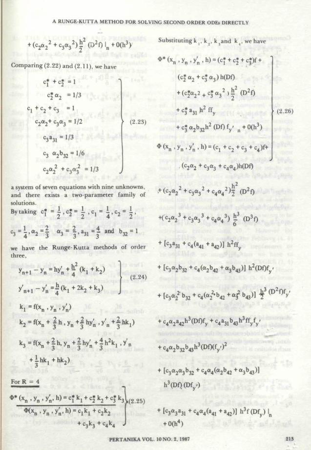
Comparing (2.22) and (2.11), we have

c* + c* = 1i i

c j o , =1/3

C l + c 2 + c3 =1

C 2 a 2 + C 3 a 3 = X>2

c3a31 = 1/3

C3 a 2 b 32 =

3 a 32 • 1/3

(2.23)

Substituting k r k2 , k 3 and k4 , we have

( c | a 2 + c * a 3 ) h ( D f )

+ (c|a22 + c*a32)ll2 (D20

+ c*a31h2ffy

+ c*a,b,,h2(Df)f' +0(h3)

3 2 3 2 v Y n v /

* (Xn > vn > *n > h> = ( c l + C2 + C3 + C4>f+

• <c2a2 + C3a3 + c4a4)h(Df)

(2.26)

a system of seven equations with nine unknowns, , 2 . 2and there exists a two-parameter family of 2 2 3 3 4solutions.

By taking c* = I , c* = I , cx = I , c2 = i , 3 + c a 3 + 3, h3

= 1 = 2 = 2 = 4 a n d b ^ ^ ^ ^C3 4 ' a 2 3 a 3 3 ' a31 3 a n 32

we have the Runge-Kutta methods of order + fC3a31 + C4<a41 + a 42^ h 2 f fy

three,

)o (D2f)

(2.24)

k i= f ( xn'yn .y;)

k-i = f(x + - h , y +4 hyl , y' + — hk1)

k 3 =f(x n + |h ,y n + |hy^ + |h 2 k 1 ,y ' n

+ Ihk1+hk2)

For R = 4

[c 3 a 2 b 3 2 + c 4 (a 2 b 4 2 + a 3 b 4 3 ) ] h2(Df)fy-

[c3a22'b32 + C 4( a 2 2 ' b 42 + a 3 2 b 43) l

C4 2 42 vUI/xy C4 d31 43 y 3

c 4a 2b 3 2b 4 3h 3 (Df)(f y ' ) 2

[ c 3 a 2 a 3 b 3 2 + c 4 a 4 ( a 2 b 4 2 + a 3 b 4 3 )

• c3k3 + c4k4 ^

+ [c3a3a31 + c4a4(a41 +a42)] h3f(Dfy) ln

+ 0(h4)

PERTANIKA VOL. 10 NO. 2, 1987 213


Comparing (2.26) with (2.11), we have~* + ~* + ~ * — i

1 2 1 ~~

c*«2 + c*a3 = l/3

c^a7 1- c a , - l/o

Cj +C 2

c2a2 +

C2a2"2 '

C 2 a 2 3 •

C3*

+ C :

c3a.

H C 3 <

hc3<

C3 a31 :

«2b32 "

! + c 4

3 + C 4 « 4

*32 + C 4

*33 + C 4

= 1/6

1/12

«42

= 1

= 1/2

= 1/3

= 1/4

c 3 a 3 1 + c 4 ( a 4 1 + a 4 2 ) =1/3

c3a2b32 + c4 (a2b42

c4a4(a2b4 2

- 1/6

C4a2a42

C4a31b43

C4 a2b32b43

C3 a3 a31 + C 4 a 4 <a41 + a42)

= 1/12

= 1/12

= 1/24

= 1/4

!= 1/8

U'

A system of 17 equations with 16 unknowns. It ispossible by careful choice of the values of the un-knowns to render some of the equations redundant, permitting the existence of a solution. Onesuch solution is

C l " = I ' C2 = 2 >C* = 6 ' W '

Then

(2.28)

For local error (I.e.) control of the computedsolution, a third order formula of the y is

} n

required. Keeping k ( and k ; the same, the firsttwo equations of (2.23) give us the formula

Then the Le. ^ Jn { - y n r This is the localerror for y^ |g Taking yn (as the solution at x^+ )

is the extrapolated solution.

For a system of equations,

3f.define —L = [

9y(j)

3f. 3f,

3y/j)

, j=0 , 1

and the operators L and D to be

L= A + y ' T 3_+ fT -L- D =3 b '3x 3y by dx

fn

Lj is the operator obtained by expanding D'and then replace y' and I by y' and f respectively.

The same result then follows.


A RUNGE KUTTA METHOD FOR SOLVING SECOND ORDER ODEs DIRECTLY

3. THE ALGORITHM AND PROBLEMSTESTED

The following algorithm is used, and is calledthe EXGRK (3, 4) method, i.e. the extrapolatedgeneralised Runge-Kutta methods of order 3 and4.Step 1: Choose tolerance, €Step 2: Put x = a, y - H , y' = TJ ' ,

r o J o 7 o

h = 0.2.€w

Step 3: Putn = 0Step 4: Put x = x + h

r n + 1 n

Step 5: If x n + ] > b goto step 9Step 6: Evaluate kJf k2, k.^ k 4and then find

Evaluate "T" andh |

5 = 0.5(f—)*

Step 7: If 8 < 0.1,IfO.K 5 < 2If 5 >2

h ->0.1hh -* 5hh -*2h

Step 8: If r n + ] > e go to step 4, i.e. reject ya + 1 .I f r n l < e , n - > > n + l and go to step 4.

Step 9: yn+1is the extrapolated value.

The following single equations were used onthe code EXGRK (3, 4) developed.

Problem 1,

y " = - y , y(0) = 0,y'(0) = 1, 0 < x < 20Theoretical solutions;y(x) = sin xy' (x) = cos x

Problem 2,y " ^ - y + x,y(0) = l , y ' ( 0 ) = 2,0 < x < 2 0Theoretical solutions;

yw -y'(x) --

Problem 3,

y'' •• =y'(0)

S i n X T C O b A T A

= cos x — sin x + 1

-300xy' - 300y, y(0) = 1,= 0, 0 < x < 10

Theoretical solutions

y(x) =

y'(x)

i- 150x

= - 3 0 0 x e 15Ox

EPSNCOUN1NFAIL

NFEVAL

EMAX

Method

Al

Problem 4,

y " = - ( n - + 0.000l)y +0.0001 sin 7T x ,

y(0) = 0,y'(0) = 7Tt0 < X<TT

Theoretical solutions,y(x) = sin TT xy'(x) » cos TTX

Using the EXGRK (3, 4) algorithm describ-ed, (1.1) was solved and compared with theRunge-Kutta —Fehberg (4, 5) method given inFehlberg (1970) using the same stepsize strategyas the above algorithm when (1.1) is reduced to asystem of first order equations. One reason whythe Fehlberg (4, 5) method is being comparedwith is that it is currently one of the mostpopular Runge-Kutta class of methods beingused to solve first order system. The results arefound in the Appendix and were obtained usingtheUNIVAC-SPERRY 1100.

In discussing the result one should bear inmind the Fehlberg (4, 5) method is of higherorder, so we should expect a better performanceover the EXGRK (3, 4) method. This seems to bethe case over all the four problems tested, fortolerances greater than 10 h However fortolerances 10 band smaller, the Fehlberg (4, 5)method exceeds either 2000 stepfailures or10,000 steps so much so that we have toterminate the program, whilst the EXGRK (3, 4)completes the range of integration. Hencedespite the low order, EXGRK (3, 4) performscreditably at finer tolerances, but less efficientlyat crude tolerances.

APPENDIX:The following results for the 4 test problems wereobtained using the Runge-Kutta-Fehlbergalorithm and the algorithm which has beenderived with the following headings:

tolerant selected,number of steps counted,number of failed steps andrejected,

number of function evaluations,local errorJy (x J - yjj, wherey(x) is the true solution and y isthe calculated solution.

Solved by the first order system

PERTANIKA VOL. 10 NO. 2, 1987 215


using Runge-Kutta-Fehlberg 'too much work" is defined for the methodalgorithm for system of equa- which require more than 10,000 steps or pro-tions. duces more than 2,000 failed steps (when yn + 1is

A2 Solved directly without using y' rejected),to approximate error.

TABLE 1The numerical result for problem 1

log, method NCOUNT NFAIL NFEVAL EMAX

- 4

- 8

Al

A2

Al

A2

Al

A2

Al

A2

17

69

47

311

144

1219

too much work

3180

0

5

0

5

0

199

(NFAIL > 2000)

1119

108

296

288

1264

870

2672

17196

0.8255 X 10

0.1228 X 10

0.3119 X 10

0.5256 X 10

0.5431 X 10

0.4499 X 10

0.340 X 10 7


log EPS method NCOUNT NFAIL NFEVAL EMAX

- 2

- 4

- 6

- 8

Al

A2

Al

A2

Al

A2

Al

A2

19

75

51

350

too much

1267

too much

1961

0

1

0

2

work (NFAIL >

704

work (NFAIL >

590

2600)

i 2000)

120

304

32

1408

7884

10204

0.7730

0.1689

03259

0.5817

0.6204

0.4528

X

X

X

X

X

X

10

10

10"

10

10

10

_ o


- 2

- 4

- 6

- 8

Al

A2

Al

A2

Al

A2

Al

A2

4044

5601

4079

5710

too much work

6081

too much work

6706

779

683

745

702

(NFAIL >

861

(NFAIL >

1018

2000)

2000)

34270

25136

24480

25648

27768

30896

0.1577

0.9267

0.2161

0.5512

0.8661

0.7171

xX

X

X

X

X

10 -<

10 ~2

10 6

10 4

10 -b

10 ~b




log, method NCOUNT NFAIL NFEVAL EMAX

- 2

- 4

- 6

- 8

Al

A2

Al

A2

Al

A2

Al

A2

47

189

140

839

8

2

0

1

too much work (NFAIL > 2000)




288

764

846

3576

0.1875 x 10"'

0.1416 X 10°

0.7726 X 10 "4

0.4837 X 10 "2

REFERENCES

FEHLBERG, E. (1964): 'New Higher Order Runge-Kutta Formulas with Step-Size Control forSystems of First-and Second-Order DifferentialEquations1 ZAMM, 44: 17 - 29.

FEHLBERG. E. (1970): 'Klassiche Runge-Kutta For-melar Vierten und Niedrigerer Ordnung mitSchitt WeitenKontrolle und thre An wendung

auf Warmeleitung-Sproblems' Computing,61-71.

6:

SULEIM AN, M. B. (1979): Generalised MultistepAdams and Backward Differentiation MethodsFor the Solution of Stiff and Non-Stiff ODEs,Ph.D. Thesis, University of Manchester.

(Received 15 October, 1986)

PERTANIKAVOL. 10 NO 2, 1987 217

a runge-kutta method for solving second order odes directly papers/pert vol. 10 (2) aug....

Documents