a robust linear least-squares estimation of camera exterior orientation using multiple geometric
TRANSCRIPT

Ž .ISPRS Journal of Photogrammetry & Remote Sensing 55 2000 75–93www.elsevier.nlrlocaterisprsjprs
A robust linear least-squares estimation of camera exteriororientation using multiple geometric features
Qiang Ji a,), Mauro S. Costa b, Robert M. Haralick b, Linda G. Shapiro b
a Department of Computer Science, UniÕersity of NeÕada at Reno, Reno, NV 89557, USAb Department of Electrical Engineering, UniÕersity of Washington Seattle, WA 98195, USA
Abstract
Ž .For photogrammetric applications, solutions to camera exterior orientation problem can be classified into linear directand non-linear. Direct solutions are important because of their computational efficiency. Existing linear solutions suffer fromlack of robustness and accuracy partially due to the fact that the majority of the methods utilize only one type of geometricentity and their frameworks do not allow simultaneous use of different types of features. Furthermore, the orthonormalityconstraints are weakly enforced or not enforced at all. We have developed a new analytic linear least-squares framework fordetermining camera exterior orientation from the simultaneous use of multiple types of geometric features. The techniqueutilizes 2Dr3D correspondences between points, lines, and ellipse–circle pairs. The redundancy provided by differentgeometric features improves the robustness and accuracy of the least-squares solution. A novel way of approximatelyimposing orthonormality constraints on the sought rotation matrix within the linear framework is presented. Results fromexperimental evaluation of the new technique using both synthetic data and real images reveal its improved robustness andaccuracy over existing direct methods. q 2000 Elsevier Science B.V. All rights reserved.
Keywords: exterior orientation; linear methods; least-squares; orthonormality constraints; feature fusion
1. Introduction
Camera exterior orientation estimation is an es-sential step for many photogrammetric applications.It addresses the issue of determining the exterior
Ž .parameters position and orientation of a camerawith respect to a world coordinate frame. Solutionsto the exterior orientation problem can be classified
) Corresponding author. Tel.: q1-775-784-4613; fax: q1-775-784-1877.
Ž .E-mail address: [email protected] Q. Ji .
into linear and non-linear methods. Linear methodshave the advantage of computational efficiency, butthey suffer from lack of accuracy and robustness.Non-linear methods, on the other hand, offer a moreaccurate and robust solution. They are, however,computationally intensive and require initial esti-mates. The classical non-linear photogrammetric ap-
Žproach to exterior orientation e.g. the bundle adjust-.ment method requires setting up a non-linear least-
squares system. Given initial estimates of the exte-rior parameters, the system is then linearized andsolved iteratively. While the classical techniqueguarantees the orthonormality of the rotation matrixand delivers the best answer, it, however, requires
0924-2716r00r$ - see front matter q 2000 Elsevier Science B.V. All rights reserved.Ž .PII: S0924-2716 00 00009-5

( )Q. Ji et al.r ISPRS Journal of Photogrammetry & Remote Sensing 55 2000 75–9376
good initial estimates. It is a well-known fact that theinitial estimates must be close or the system may notconverge quickly or correctly. Hence, the quality ofinitial estimates is critical since it determines theconvergence speed and the correctness of the itera-tive procedure. Robust and accurate linear solutions,which are often used to provide initial guesses fornon-linear procedures, are therefore important forphotogrammetric problems.
Numerous methods have been proposed to analyt-ically obtain camera exterior parameters. Previousmethods have primarily been focused on using setsof 2D–3D point correspondences to solve for thetransformation matrix, followed by extracting thecamera parameters from the solved transformation.The linear method using points is well known inphotogrammetry as direct linear transformation( )DLT .
The original proposal of DLT method appears inŽ .Abdel-Aziz and Karara 1971 . Since then, different
variations of DLT methods have been introduced.Ž .For example, Bopp and Krauss 1978 published a
variation of the DLT, incorporating added constraintsŽ .into the solution. Okamoto 1981 gave an alterna-
tive derivation of the DLT from a more generalŽ .mathematical framework. Shan 1996 introduced a
linear solution for object reconstruction from a stere-opair without interior orientation and less require-ments on known points than the original DLT formu-lation.
In computer vision, the DLT-like methods includeŽ .the three-point solution Fischler and Bolles, 1981 ,Žthe four-point solutions Hung et al., 1985; Holt and
.Netravali, 1991 , and the six- or more-point solutionsŽ .Sutherland, 1974; Tsai, 1987; Faugeras, 1993 . Har-
Ž .alick et al. 1994 reviewed and compared majordirect solutions of exterior orientation using three-point correspondences and characterized their perfor-mance under varying noisy conditions. SutherlandŽ .1974 provided a closed-form least-squares solutionusing six or more points. The solution, however, is
Ž .only up to a scale factor. Faugeras 1993 proposed asimilar technique that solves the scale factor byapplying a normality constraint. His solution alsoincludes a post-orthogonalization process that en-sures the orthonormality of the resulting rotation
Ž .matrix. Tsai 1987 presented a direct solution bydecoupling the camera parameters into two groups;
each group is solved for separately in different stages.While efficient, Tsai’s method does not impose anyof the orthonormal constraints on the estimated rota-tion matrix. Also, the errors with the camera parame-ters estimated in the earlier stage can significantlyaffect the accuracy of parameters estimated in thelater stage.
These methods are effective and simple to imple-ment. However, they are not robust and are very
Žsusceptible to noise in image coordinates Wang and.Xu, 1996 , especially when the number of control
points approaches the minimum required. For theŽ .three-point solutions, Haralick et al. 1994 show
that even the order of algebraic substitutions canrender the output useless. Furthermore, the pointdistribution and noise in the point coordinates canalso dramatically change the relative output errors.For least-squares-based methods, a different study by
Ž .Haralick et al. 1989 show that when the noise levelexceeds certain level or the number of points isbelow certain level, these methods become extremelyunstable and the errors skyrocket. The use of morepoints can help relieve this problem. However, gen-eration of more control points often proves to bedifficult, expensive, and time-consuming. Anotherdisadvantage of point-based methods is the difficultywith point matching, i.e., finding the correspon-dences between the 3D scene points and 2D imagepixels.
In view of these issues, other researchers haveinvestigated the use of higher-level geometric fea-tures such as lines or curves as observed geometricentities to improve the robustness and accuracy oflinear methods for estimating exterior parameters.Over the years, various algorithms using featuresother than points for exterior orientation problemshave been introduced both in photogrammetry and
Žcomputer vision Doehler, 1975; Haralick and Chu,1984; Paderes et al., 1984; Mulawa, 1989; Mulawaand Mikhail, 1988; Tommaselli and Lugnani, 1988;Chen and Tsai, 1990, 1991; Echigo, 1990; Lee et al.,1990; Liu et al., 1990; Wang and Tsai, 1990; Fin-sterwalder, 1991; Heikkila, 1991; Rothwell et al.,1992; Weng et al., 1992; Mikhail, 1993; Petsa and
. Ž .Patias, 1994a,b . In photogrammetry, Strunz 1992gives a good overview of using various featuresŽ .points, lines, and surfaces for different photogram-metric tasks, including camera orientation. Szczepan-

( )Q. Ji et al.r ISPRS Journal of Photogrammetry & Remote Sensing 55 2000 75–93 77
Ž .ski 1958 reviewed nearly 60 different solutions forspace resection, dating back to 1829, for the simulta-neous and separate determination of the position androtation parameters. An iterative Kalman filteringmethod for space resection using straight-line fea-
Ž .tures was described in Tommaselli and Tozzi 1996 .Ž .Masry 1981 described a method for camera abso-
Ž .lute orientation and Lugnani 1980 for camera exte-rior orientation by spatial resection, using linear
Ž .features. Drewniok and Rohr 1997 presented anapproach for automatic exterior orientation of aerialimagery that is based on detection and localisation of
Ž . Ž .planar objects manhole covers . Ethrog 1984 usedparallel and perpendicular lines of objects for estima-tion of the rotation and interior orientation of non-metric cameras.
Researchers have also used other known geomet-ric shapes in the scene to constrain the solution. Such
Ž .shapes can be 2D straight lines, circles, etc. or 3DŽ . Žfeatures on a plane, cylinder, etc. Mikhail and
. ŽMulawa, 1985 . Others Kruck, 1984; Kager, 1989;
.Forkert, 1996 have incorporated geometric con-straints such as coordinate differences, horizontaland space distances, and angles to improve the tradi-
Ž .tional bundle adjustment method. Heikkila 1990 ,Ž . Ž .Pettersen 1992 , and Maas 1999 employed a mov-
Ž .ing reference bar known distance for camera orien-tation and calibration.
Ž .In computer vision, Haralick and Chu 1984presented a method that solves the camera exteriorparameters from the conic curves. Given the shape ofconic curves, the method first solves for the threerotation parameters using an iterative procedure. Thethree translation parameters are then solved analyti-cally. The advantage of this method is that it doesnot need to know the location of the curves and it ismore robust than any analytical method in that rota-tion parameter errors are reduced to minimum beforethey are used analytically to compute translation
Ž .parameters. In their analytic method, Liu et al. 1990Ž .and Chen and Tsai 1990 discussed direct solutions
for determining camera exterior parameters based ona set of 2D–3D line correspondences. The key totheir approach lies in the linear constraint they used.This constraint uses the fact that a 3D line and itsimage line lie on the same plane determined by thecenter of perspectivity and the image line. Rothwell
Ž .et al. 1992 discussed a direct method that deter-
mines camera parameters using a pair of conic curves.The method works by extracting four or eight pointsfrom conic intersections and tangencies. Exteriorcamera parameters are then recovered from these
Ž .points. Kumar and Hanson 1989 described a robusttechnique for finding camera parameters using lines.
Ž .Kamgar-Parsi and Eas 1990 introduced a cameracalibration method with small relative angles. GaoŽ .1992 introduced a method for estimating exteriorparameters using parallelepipeds. Forsyth et al.Ž .1991 proposed to use a pair of known conics or asingle known circle for determining the pose of the
Ž .object plane. Haralick 1988 and Haralick and ChuŽ .1984 presented methods for solving for cameraparameters using rectangles and triangles. AbidiŽ .1995 presented a closed form solution for poseestimation using quadrangular targets. Linnainmaa
Ž .and Harwood 1988 discussed an approach for de-termination of 3D object using triangle pairs. Chen
Ž .and Tsai 1991 proposed closed solution for poseestimation from line-to-plane correspondences andstudied the condition of the existence of the closed
Ž .solution. Ma 1993 introduced a technique for poseestimation from the correspondence of 2Dr3D con-ics. The technique, however, is iterative and requiresa pair of conics in both 2D and 3D.
Analytic solutions based on high-level geometricfeatures afford better stability and are more robustand accurate. Here, the correspondence problem canbe addressed more easily than for the point-basedmethods. However, high-level geometric featuresmay not always be present in some applications, andpoints are present in many applications. Therefore,completely ignoring points while solely employinghigh-level geometric entities can be a waste of read-ily available geometric information. This is one ofthe problems with the existing solutions: they eitheruse points or lines or conics but not a combination offeatures. In this paper, we describe an integratedleast-squares method that solves for the cameratransformation matrix analytically by fusing avail-able observed geometric information from differentlevels of abstraction. Specifically, we analyticallysolve for the exterior parameters from simultaneoususe of 2D–3D correspondences between points, be-tween lines, and between 2D ellipses and 3D circles.The attractiveness of our approach is that the redun-dancy provided by features at different levels im-

( )Q. Ji et al.r ISPRS Journal of Photogrammetry & Remote Sensing 55 2000 75–9378
proves the robustness and accuracy of the least-squares solution, therefore improving the precisionof the estimated parameters. To our knowledge, noprevious research attempts have been made in devel-oping a linear solution to exterior orientation withsimultaneous use of all three classes of features.
Ž .Work by Phong et al. 1995 described a techniquein which information from both points and lines isused to compute the exterior orientation. However,the method is iterative and involves only points andlines.
Another major factor that contributes to the lackof robustness of the existing linear methods is thatorthonormality constraints on the rotation matrix areoften weakly enforced or not enforced at all. In thisresearch, we introduce a simple, yet effective, schemefor approximately imposing the orthonormal con-straints on the rotation matrix. While the schemedoes not guarantee that the resultant rotation matrixcompletely satisfies the orthonormal constraints, itdoes yield a matrix that is closer to orthonormalitythan those obtained with competing methods.
This paper is organized as follows. Section 2briefly summarizes the perspective projection geom-etry and equations. Least-squares frameworks forestimating the camera transformation matrix from2D–3D point, line, and ellipsercircle correspon-dences are presented in Sections 3–5, respectively.Section 6 discusses our technique for approximatelyimposing orthonormal constraints and presents theintegrated linear technique for estimating the trans-formation matrix simultaneously using point, line,and ellipsercircle correspondences. Performancecharacterization and comparison of the developedintegrated technique is covered in Section 7.
2. Perspective projection geometry
To set the stage for the subsequent discussion,this section briefly summarizes the pin–hole cameramodel and the perspective projection geometry.
Ž . tLet P be a 3D point and x y z be the coordi-nates of P relative to the object coordinate frameC . Define the camera coordinate system C to haveo c
its z-axis parallel to the optical axis of the cameralens and its origin located at the perspective center.
Ž . tLet x y z be the coordinates of P in C .c c c c
Define C to be the image coordinate system, with itsi
u-axis and Õ-axis parallel to the x- and y-axes of thecamera coordinate frame, respectively. The origin of
Ž . tC is located at the principal point. Let u Õ be thei
coordinates of P , the image projection of P in C .i i
Fig. 1 depicts the pin–hole camera model.Based on the perspective projection theory, the
Ž .projection that relates u,Õ on the image plane toŽ .the corresponding 3D point x , y , z in thec c c
camera frame can be described by
xu c
Õl s 1Ž .yc� 0 � 0f zc
where l is a scalar and f is the camera focal length.Ž . t Ž . tFurther, x y z relates to x y z by a rigidc c c
body coordinate transformation consisting of a rota-tion matrix and a translation. Let a 3=3 matrix Rrepresent the rotation and a 3=1 vector T describethe translation, then
xc xsR qT 2Ž .y yc ž /� 0 zzc
Žwhere T and R can be parameterized as Ts t tx y. tt andz
r r r11 12 13
Rs r r r21 22 23� 0r r r31 32 33
R and T describe the orientation and location of theobject frame relative to the camera frame, respec-tively. Together, they are referred to as the camera
Fig. 1. Camera and perspective projection geometry.

( )Q. Ji et al.r ISPRS Journal of Photogrammetry & Remote Sensing 55 2000 75–93 79
transformation matrix. Substituting the parameter-Ž .ized T and R into Eq. 2 yields
tx r r r xc 11 12 13 xts q 3Ž .y r r r y yc 21 22 23 ž /� 0 � 0 � 0zz r r r tc 31 32 33 z
Ž .Combining the projection Eq. 1 with the rigidŽ .transformation of Eq. 2 and eliminating l yields
the collinearity equations, which describe the idealrelationship between a point on the image plane andthe corresponding point in the object frame
r xqr yqr zq t11 12 13 xus f 4Ž .
r xqr yqr zq t31 32 33 z
r xqr yqr zq t21 22 23 yÕs f
r xqr yqr zq t31 32 33 z
For a rigid body transformation, the rotation ma-trix R must be orthonormal, that is, R t sRy1. Theconstraint R t sRy1 amounts to the six orthonormal-ity constraint equations on the elements of R
r 2 qr 2 qr 2 s1 r r qr r qr r s011 12 13 11 21 12 22 13 23
2 2 2r qr qr s1 r r qr r qr r s021 22 23 11 31 12 32 13 33
2 2 2r qr qr s1 r r qr r qr r s031 32 33 21 31 22 32 23 33
5Ž .
where the three constraints on the left column arereferred to as the normality constraints and the threeon the right column as the orthogonality constraints.
The normality constraints ensure that the row vectorsof R are unit vectors, while the orthogonality con-straints guarantee orthogonality among row vectors.
3. Camera transformation matrix from point cor-respondences
Given the 3D object coordinates of a number ofpoints and their corresponding 2D image coordi-nates, the coefficients of R and T can be solved forby a least-squares solution of an over-determinedsystem of linear equations. Specifically, the least-squares method based on point correspondences canbe formulated as follows.
Ž .Let X s x , y , z , ns1, . . . , K , be the 3Dn n n n
coordinates of K points relative to the object frameŽ .and U s u , Õ be the observed image coordinatesn n n
of these points. We can then relate X and U vian nŽ .the collinearity equations in Eq. 4 . Rewriting Eq.
Ž .4 yields
fr x q fr y q fr z yu r x yu r y11 n 12 n 13 n n 31 n n 32 n
yu r z q ft yu t s0 6Ž .n 33 n x n z
fr x q fr y q fr z yu r x yÕ r y21 n 22 n 23 n n 31 n n 32 n
yÕ r z q ft yu t s0n 33 n y n z
We can then set up a matrix M and a vector V asfollows
fx fy fz 0 0 0 yu x yu y yu z f 0 yu1 1 1 1 1 1 1 1 1 1
0 0 0 fx fy fz yÕ x yÕ y yÕ z 0 f yÕ1 1 1 1 1 1 1 1 1 1.
2 K=12 .M s 7Ž ..fx fy fz 0 0 0 yu x yu y yu z f 0 yuK K K K K K K K K K� 00 0 0 fx fy fz yu x yÕ y yÕ z 0 f yÕK K K K K K K K K K
t12=1 r r r r r r r r r t t tV s 8Ž .11 12 13 21 22 23 31 32 33 x y zž /
where M is hereafter referred to as the collinearitymatrix and V is the unknown vector of transforma-
tion parameters containing all sought rotational andtranslational coefficients.

( )Q. Ji et al.r ISPRS Journal of Photogrammetry & Remote Sensing 55 2000 75–9380
To determine V , we can set up a least-squaresproblem that minimizes
2 5 5 2j s MV 9Ž .
where j 2 is the sum of squared residual errors of allpoints. Given an overdetermined system, a least-squares solution to the above equation requires mini-
5 5 2mization of MV . Its solution contains an arbi-trary scale factor due to the lack of constraints on R.To uniquely determine V , different methods havebeen proposed to solve for the scale factor. In the
Ž .least-squares solution provided by Sutherland 1974 ,the depth of the object is assumed to be unity; t s1.z
Not only is this assumption unrealistic for mostapplications, but also the solution is constructedwithout regard to the orthonormal constraints that R
Ž .must satisfy. Faugeras 1993 posed the problem as aconstrained least-squares problem using a minimum
Žof six points. The third normality constraint the last. Ž .one on the left column in Eq. 5 is imposed by
Faugeras during the minimization to solve for thescale factor and to constrain the rotation matrix. Thelinearity in solution is preserved due to the use of asingle normality constraint.
4. Camera transformation matrix from line corre-spondences
Given correspondences between a set of 3D linesand their observed 2D images, we can set up asystem of linear equations that involve R, T , and thecoefficients for 3D and 2D lines as follows. Let a 3Dline L in the object frame be parametrically repre-sented as
L: XslNqP
Ž . twhere Xs x y z is a generic point on the line, l
is a scalar representing the signed distance fromŽ . tpoint P to point X, Ns A B C is the known
Ž . tdirection cosine vector and Ps P P P is ax y z
known point on the line relative to the object frame.Let the corresponding 2D line l on the image planebe represented by
l : auqbÕqcs0
Fig. 2. Projection plane formed by a 2D image line l and thecorresponding 3D line L.
Ideally, the 3D line must lie on the projection planeformed by the center of perspectivity and the 2Dimage line as shown in Fig. 2.
Relative to the camera frame, the equation of theprojection plane can be derived from the 2D lineequation as
afx qbfy qcz s0c c c
where f is the focal length. Since the 3D line lies onthe projection plane, the plane normal must be per-pendicular to the line. Denote the plane normal by
t 2 2 2 2 2Ž . (ns af ,bf ,c r a f qb f qc ; then given anideal projection, we have
nt R Ns0 10Ž .Similarly, since point P is also located on theprojection plane, this leads to
nt R PqT s0 11Ž . Ž .Ž . Ž .Eqs. 10 and 11 are hereafter referred to as copla-
narity equations. Equivalently, they can be rewrittenas
A a r qB a r qC a r qA b r qB b r11 12 13 21 22
qC b r qA c r qB c r qC c r s023 31 32 33
P a r qP a r qP a r qP b r qP b rx 11 y 12 z 13 x 21 y 22
qP b r qP c r qP c r qP c r qa tz 23 x 31 y 32 z 33 x
qb t qc t s0y z

( )Q. Ji et al.r ISPRS Journal of Photogrammetry & Remote Sensing 55 2000 75–93 81
Given a set of J line correspondences, we can set upa system of linear equations similar to those for
points that involve matrix H and vector V , where Vis as defined before and H is defined as follows
A a B a C a A b B b C b A c B c C c 0 0 01 1 1 1 1 1 1 1 1 1 1 1 1 1 1 1 1 1
P a P a P a P b P b P b P b P c P c a b cx 1 y 1 z 1 x 1 y 1 z 1 x 1 y 1 z 1 1 1 11 1 1 1 1 1 1 1 1.
2 J=12 .H s 12Ž ..A a B a C a A b B b C b A c B c C c 0 0 0J J J J J J J J J J J J J J J J J J� 0P a P a P a P b P b P b P c P c P c a b cx J y J z J x J y J z J x J Y J z J J J JJ J J J J J J J J
and is called the coplanarity matrix. Again we cansolve for V by minimizing the sum of squared
5 5 2residual errors HV . V can be solved for up to ascale factor. The scale factor can be determined byimposing one of the normality constraints as dis-cussed for the case using points.
5. Camera transformation matrix from ellipse–circle correspondences
5.1. Camera transformation matrix from circles
Ž .Given the image an ellipse of a 3D circle and itsŽ .size, the pose position and orientation of the 3D
circle relative to the camera frame can be solved foranalytically. Solutions to this problem may be found
Ž . Ž .in Haralick and Shapiro 1993 , Forsyth et al. 1991 ,Ž .and Dhome et al. 1989 . If we are also given the
pose of the circle in the object frame, then we canuse the two poses to solve for R and T. Specifically,
Ž . t Ž . tlet N s N N N and O s O O O bec c c c c c c cx y z x y z
the 3D circle normal and center in the camera coor-Ždinate frame respectively. Also, let N s N No o ox y
. t Ž . tN and O s O O O be the normal ando o o o oz x y z
center of the same circle, but in the object coordinatesystem. O and N are computed from the observedc c
image ellipse using a technique described in ForsythŽ .et al. 1991 , while N and O are assumed to beo o
known. The problem is to determine R and T fromthe correspondence between N and N , and be-c o
tween O and O . The two normals and the twoc o
centers are related by the transformation R and T asshown below
No xr r r11 12 13
NN sR N s 13Ž .or r r yc o 21 22 23� 0 � 0r r r31 32 33 No z
and
O to xr r r x11 12 13
O tO sRO qTs qor r r yyc o 21 22 23� 0 � 0� 0r r r t31 32 33 O zo z
14Ž .
Ž . Ž .Equivalently, we can rewrite Eqs. 13 and 14 asfollows
N r qN r qN r sNo 11 o 12 o 13 cx y z x
N r qN r qN r sNo 21 o 22 o 23 cx y z y
N r qN r qN r sNo 31 o 32 o 33 cx y z x
and
O r qO r qO r q t sOo 11 o 12 o 13 x cx y x x
O r qO r qO r q t sOo 21 o 22 o 23 y cx y x y
O r qO r qO r q t sOo 31 o 32 o 33 z cx y x z
Each pair of 2D ellipse and 3D circle therefore offerssix equations. The three equations from orientationŽ Ž ..Eq. 13 are not independent due to unity constrainton the normals. Given I observed ellipses and their

( )Q. Ji et al.r ISPRS Journal of Photogrammetry & Remote Sensing 55 2000 75–9382
corresponding object space circles, we can set up asystem of linear equations to solve for R and T by
5 5 2minimizing the sum of residual errors QVyk ,where Q and k are defined as follows
° ¶N N N 0 0 0 0 0 0 0 0 01 1 1o o ox y z
0 0 0 N N N 0 0 0 0 0 01 1 1o o ox y z
0 0 0 0 0 0 N N N 0 0 01 1 1o o ox y z
O O O 0 0 0 0 0 0 1 0 01 1 1o o ox y z
0 0 0 O O O 0 0 0 0 1 01 1 1o o ox y z
0 0 0 0 0 0 O O O 0 0 11 1 1o o ox y z
.6 I=12 .Q s 15Ž ..
N N N 0 0 0 0 0 0 0 0 0I I Io o ox y z
0 0 0 N N N 0 0 0 0 0 0I I Io o ox y z
0 0 0 0 0 0 N N N 0 0 0I I Io o oz y z
O O O 0 0 0 0 0 0 1 0 0I I Io o ox y z
0 0 0 O O O 0 0 0 0 1 0I I Io o ox y z
0 0 0 0 0 0 O O O 0 0 1¢ ßI I Io o ox y z
and
t6 I=1 N N N O O O . . . N N N O O O1 1 1 1 1 1 I I I I I Ik s 16Ž .c c c c c c c c c c c cx y z x y z x y z x y zž /
Since each circle provides six equations, a minimumŽ .of two circles are needed if only circles are used to
uniquely solve for the 12 parameters in the transfor-mation matrix. To retain a linear solution, not evenone normality constraint can be imposed using La-grange multipliers due to k being non-zero vector.
6. The integrated technique
In the previous sections, we have outlined theleast-squares frameworks for computing the transfor-mation matrix from different features individually. Itis desirable to be able to compute camera exteriorparameters using more than one type of featuresimultaneously. In other words, given observed geo-
metric entities at different levels, we want to developa mechanism that systematically and consistentlyfuses this information. The reason is quite obvious:using all available geometric information will pro-vide a more accurate and robust solution, since itincreases the redundancy of the least-squares estima-tion. It also reduces the dependency on points. Wecan be more selective when choosing points, withoutworrying about the minimum number of pointsneeded for accurate results. Furthermore, we canworry less about whether the selected points arecoplanar or not and their distribution. This section isdevoted to formulating a direct solution for comput-ing camera transformation matrix from the simulta-neous use of 2D–3D correspondences of points,lines, and ellipsesrcircles.

( )Q. Ji et al.r ISPRS Journal of Photogrammetry & Remote Sensing 55 2000 75–93 83
6.1. Fusing all obserÕed information
The problem of integrating information frompoints, lines, and circles is actually straightforward,given the frameworks we have outlined individuallyfor points, lines, and circles. The problem can bestated as follows.
Given the 2D–3D correspondences of K points,J lines, and I ellipsercircle pairs, we want to set upa system of linear equations that involves all geomet-ric entities. The problem can be formulated as aleast-squares estimation in the form of minimizing5 5WVyb , where V is the unknown vector of trans-formation parameters as defined before, and b is aknown vector defined below. W is an augmentedcoefficient matrix, whose rows consist of linearequations derived from points, lines, and circles.Specifically, given the M, H, and Q matrices defined
Ž Ž . Ž . Ž .in Eqs. 7 , 12 and 15 , the W matrix is
MŽ2 Kq2 Jq6 I .=12W s 17Ž .Hž /Q
where the first 2 K rows of W represent contribu-tions from points, the second subsequent 2 J rowsrepresent contributions from lines, and the last 6 Irows represent contributions from circles. The vectorb is defined as
tŽ2 Kq2 Jq6 I .=1b s 180 0 0 . . . kŽ . Ž .Ž .where k is defined in Eq. 16 . Given W and b, the
least-squares solution to V isy1t tVs W W W b 19Ž . Ž .
It can be seen that to have an overdetermined systemof linear equations, we need 2 Kq2 Jq6 IG12 ob-served geometric entities. This may occur with anycombination of points, lines, and circles. For exam-ple, one point, one line, and one circle or two pointsand one circle are sufficient to solve the transforma-
Ž .tion matrix from Eq. 19 . Any additional points orlines or circles will improve the robustness and theprecision of the estimated parameters. The integratedapproach so far, however, does not impose any ofthe six orthonormality constraints. Also, we assumeequal weightings for observations from the multiplefeatures. We realize stochastic model is very impor-tant while using multiple features. As part of future
work, we plan to use error propagation to compute acovariance matrix for each type of feature. Thecovariance matrices can then be used to compute theobservation weightings.
6.2. Approximately imposing orthonormal con-straints
The least-squares solution to V described in thelast section cannot guarantee the orthonormality ofthe resultant rotation matrix. One major reason whyprevious linear methods are very susceptible to noiseis because the orthonormality constraints are notenforced or enforced weakly. To ensure this, the sixorthonormal constraints must be imposed on V withinthe least-squares framework. The conventional wayof imposing these constraints is through the use ofLagrange multipliers. However, simultaneously im-posing any two normality constraints or one orthogo-nality constraint using Lagrange multipliers requiresa non-linear solution for the problem. Therefore,most linear methods choose to use a single normality
Ž .constraint. For example, Faugeras 1993 imposedthe constraint that the norm of the last row vector ofR be unity. This constraint, however, cannot ensurecomplete satisfaction of all orthonormal constraints.To impose more than one orthonormality constraint
Ž .but still retain a linear solution, Liu et al. 1990suggested the constraint that the sum of the squaresof the three row vectors be 3. This constraint, how-ever, cannot guarantee normality of each individual
Ž . Ž .row vector. Haralick et al. 1989 and Horn 1987proposed direct solutions, where all orthonormalityconstraints are imposed, but for the 3D to 3D abso-lute orientation problem. They are only applicablefor point correspondences and are not applicable toline and circle–ellipse correspondences. Most impor-tant, their techniques cannot be applied to the generallinear framework we propose.
Given the linear framework, even imposing oneconstraint using the Lagrange multiplier can renderthe solution non-linear. It is well known that thesolution to minimizing a quadratic function with
Žquadratic constraints referred to as trust region.problem in statistics can only be achieved by non-
linear methods.We now introduce a simple, yet effective, method
for approximately imposing the orthonormal con-

( )Q. Ji et al.r ISPRS Journal of Photogrammetry & Remote Sensing 55 2000 75–9384
straints in a way that offers a linear solution. Wewant to emphasize that the technique we are about to
Ž tintroduce cannot guarantee a perfect satisfying R sy1 .R rotation matrix. However, our experimental
study proves that it yields a matrix that is closer to arotation matrix than those obtained using the compet-ing methods. The advantages of our technique are:Ž .1 all six orthonormal constraints are imposed si-
Ž .multaneously; 2 constraints are imposed on eachŽ .entry of the rotation matrix, and 3 asymptotically,
the resulting matrix should converge to a rotationmatrix. However, this method requires knowledge ofthe 3D orientation of a vector in both camera andobject frames.
We now address the problem of how to imposethe orthonormality constraints in the general frame-work of finding pose from multiple geometric fea-tures described in Sections 3–5. Given the pose ofcircles relative to the camera frame and the object
Ž . t Žframe, let N s N N N and N s N Nc c c c o o ox y z x y
. tN be the 3D circle normals in camera and objecto z
Ž .frames, respectively. Eq. 13 depicts the relation
between two normals that involves R. The relationcan also be expressed in an alternative way that
t Ž t y1.involves R note R sR as follows
Nc xr r r11 21 31t NN sR N s 20Ž .cr r r yo c 12 22 32� 0 � 0r r r13 23 33 Nc z
Ž .Equivalently, we can rewrite Eq. 20 as follows
N r qN r qN r sNc 11 c 21 c 31 ox y z x
N r qN r qN r sNc 12 c 22 c 32 ox y z y
N r qN r qN r sNc 13 c 23 c 33 ox y z z
Given the same set of I observed ellipses andtheir corresponding object space circles, we can setup another system of linear equations that uses thesame set of circles as in Q. Let QX be the coefficientmatrix that contains the coefficients of the set oflinear equations, then QX is
N 0 0 N 0 0 N 0 0 0 0 0° ¶1 1 1c c cx y z
0 N 0 0 N 0 0 N 0 0 0 01 1 1c c cx y z
0 0 N 0 0 N 0 0 N 0 0 01 1 1c c cz y z
.X 3 I=12 .Q s 21Ž ..N 0 0 N 0 0 N 0 0 0 0 0I I Ic c cx y z
0 N 0 0 N 0 0 N 0 0 0 0I I Ic c cx y z
0 0 N 0 0 N 0 0 N 0 0 0¢ ßI I Ic c cz y z
Correspondingly, we have kX defined as
tX 3 I=1 N N N 0 0 0 . . . N N N 0 0 01 1 1 I I Ik s 22Ž .o o o o o ox y z x y zž /
To implement the constraint in the least-squaresŽ .framework, we can augment matrix W in Eq. 19
with QX, yielding W X, and augment vector b in Eq.Ž . X X X X18 with k , yielding b , where W and b aredefined as follows
W bX 2 Kq2 Jq9 I=12 XŽ2 Kq2 Jq9 I .=1W s b sX Xž / ž /Q k
Putting it all together, the solution to V can be found5 X X 5 2by minimizing W Vyb , given by
y1X t X X t XVs W W W b 23Ž .Ž .
For each circle, we add three additional equations toimpose the orthonormality constraints. Therefore, thefirst 2 K rows of W X represent contributions from

( )Q. Ji et al.r ISPRS Journal of Photogrammetry & Remote Sensing 55 2000 75–93 85
points, the second subsequent 2 J rows representcontributions from lines, and the last 9I rows repre-sent contributions from circles.
We must make it clear that the proposed methodfor imposing orthonormality will not be applicable ifthe required ellipsercircle features are not available.It is only applicable to circles but not applicable topoints or lines. In this case, we can only partiallyapply the orthonormality constraints, i.e., applyingone of the normality constraints or performing apost-orthogonalization process like the one used by
Ž .Faugeras 1993 .To have an overdetermined system of linear equa-
tions, we need 2 Kq2 Jq9IG12 observed geomet-ric entities. This may occur with any combination ofpoints, lines, and circles. For example, one point,one line, and one circle or two points and one circleor even two circles are sufficient to solve for thetransformation matrix. The resultant transformationparameters R and T are more accurate and robustdue to fusing information from different sources. Theresultant rotation matrix R is also very close to beingorthonormal since the orthonormality constraints havebeen explicitly added to the system of linear equa-tions used in the least-squares estimation. The ob-tained R and T can be used directly for certain
Žapplications or fed to an iterative procedure such as.the bundle adjustment method to refine the solution.
Since the obtained transformation parameters areaccurate, the subsequent iterative procedure not onlycan converge very quickly, usually after a couple ofiterations as evidenced by our experiments but, moreimportantly, converge correctly. In the section tofollow, we study the performance of the new linearexterior orientation estimation method against themethods that use only one type of geometric entity ata time, using synthetic and real images.
7. Experiments
In this section, we present and discuss the resultsof a series of experiments aimed at characterizing theperformance of the integrated linear exterior orienta-tion estimation technique. Using both synthetic dataand real images of industrial parts, the experimentsconducted aim at studying the effectiveness of theproposed technique for approximately imposing the
orthonormal constraints and quantitatively evaluatingthe overall performance of the integrated linear tech-nique against existing linear techniques.
7.1. Performance study with synthetic data
This section consists of two parts. First, we pre-sent results from a large number of controlled exper-iments aimed at analyzing the effectiveness of ourtechnique for imposing orthonormal constraints. Thiswas accomplished by comparing the errors of theestimated rotation and translation vectors obtainedwith and without orthonormal constraints imposedunder different conditions. Second, we discuss theresults from a comparative performance study of theintegrated linear technique against an existing lineartechnique under different noisy conditions.
In the experiments with simulation data, the 3DŽdata 3D point coordinates, 3D surface normals, 3D
.line direction cosines are generated randomly withinspecified ranges. For example, 3D coordinates are
wŽ .randomly generated within the cube y5, y5, y5Ž .xto 5,5,5 . 2D data are generated by projecting the
3D data onto the image plane, followed by perturb-ing the projected image data with independently and
Ž .identically distributed iid Gaussian noise of meanvector of zero and covariance matrix of s 2 I, wheres 2 represents noise variance and I is the identitymatrix. From the generated 2D–3D data, we estimatethe rotation and the translation vector using thelinear algorithm, from which we can compute theestimation errors. The estimation error is defined asthe Euclidean distance between the estimated rota-
Ž . Žtion translation vector and the ideal rotation trans-.lation vector. We choose the rotation matrix rather
than other specific representations like Euler anglesand quaternion parameters for error analysis. This isbecause all other representations depend on the esti-mated rotation vector. For each experiment, 100
Ž .trials with different noise instances are performedand the average distance errors are computed. Thenoise level is quantified using the signal-to-noise
Ž .ratio SNR . SNR is defined as 20log drs , where s
is the standard deviation of the Gaussian noise and dis the range of the quantity being perturbed.
Figs. 3 and 4 plot the mean rotation and transla-tion errors as a function of the SNR, with andwithout orthonormal constraints imposed. It is clear

( )Q. Ji et al.r ISPRS Journal of Photogrammetry & Remote Sensing 55 2000 75–9386
Fig. 3. Mean rotation vector error versus SNR. The plot wasgenerated using the integrated linear technique with a combinationof one point, one line, and one circle. Each point in the figurerepresents an average of 100 trials.
from the two figures that imposing the orthonormalconstraints improves the estimation errors for boththe rotation and translation vectors. The improve-ment is especially significant when the SNR is low.
To further study the effectiveness of the techniquefor imposing constraints, we studied its performanceunder different numbers of pairs of ellipsercirclecorrespondences. This experiment is intended tostudy the efficacy of imposing orthonormal con-straints versus the amount of geometric data used forthe least-squares estimation. The results are plotted
Ž .Fig. 4. Mean translation vector error mm versus SNR. The plotwas generated using the integrated linear technique with a combi-nation of one point, one line, and one circle. Each point in thefigure represents an average of 100 trials.
Fig. 5. Mean rotation vector error versus the number ofŽ .ellipsercircle pairs SNRs35 .
in Figs. 5 and 6, which give the average rotation andtranslation errors as a function of the number ofellipsercircle pairs used, with and without con-straints imposed. The two figures again show thatimposing orthonormal constraints leads to an im-provement in estimation errors. This improvement,however, begins to decrease when the features usedexceed a certain number. The technique is mosteffective when fewer ellipsercircle pairs are used.
To compare the integrated linear technique withan existing linear technique, we studied its perfor-
Ž .mance against that of Faugeras 1993 . The resultsare given in Figs. 7 and 8, which plot the mean
Ž .Fig. 6. Mean translation vector error mm versus the number ofŽ .ellipsercircle pairs SNRs35 .

( )Q. Ji et al.r ISPRS Journal of Photogrammetry & Remote Sensing 55 2000 75–93 87
Fig. 7. Mean rotation vector error versus SNR. The curve forFaugeras’ algorithm was obtained using 10 points, while the curvefor the integrated technique was generated using a combination ofthree points, one line, and one circle.
rotation and translation vector errors as a function ofthe SNR, respectively.
The two figures clearly show the superiority ofthe new integrated technique over Faugeras’ lineartechnique, especially for the translation errors. Tofurther compare the sensitivity of the two techniquesto viewing parameters, we changed the position pa-rameters of the camera by doubling the cameradistance z to the object points. Figs. 9 and 10 plotthe mean rotation and translation vector errors as a
Ž .Fig. 8. Mean translation vector error mm versus SNR. The curvefor Faugeras’ algorithm was obtained using 10 points, while thecurve for the integrated technique was generated using a combina-tion of three points, one line, and one circle.
Fig. 9. Mean rotation vector error versus SNR with an increasedŽcamera position parameter z doubling the camera and object
.distance z . The curve for Faugeras’ algorithm was obtained using10 points, while the curve for the integrated technique wasgenerated using a combination of three points, one line, and onecircle.
function of SNR respectively under the new cameraposition. While increasing z causes an increase inthe estimation errors for both techniques, its impacton Faugeras’ technique is more serious. This leads toa much more noticeable performance difference be-tween the two linear techniques. The fact that the
Ž .Fig. 10. Mean translation vector error mm versus SNR with anŽincreased camera position parameter z doubling the camera and
.object distance z . The curve for Faugeras’ algorithm was gener-ated using 10 points while the curve for the integrated techniquewas generated using a combination of three points, one line, andone circle.
( )Q. Ji et al.r ISPRS Journal of Photogrammetry & Remote Sensing 55 2000 75–9388
integrated technique using only five geometric enti-Žties three points, one line, and one circle with a total
.of 17 equations still outperforms Faugeras’ tech-Ž .nique, which uses 10 points a total of 20 equations ,
shows that the higher-level geometric features suchas lines and circles can provide more robust solu-tions than those provided solely by points. Thisdemonstrates the power of combining features ondifferent levels of abstraction. Our study also showsthat Faugeras’ linear technique is very sensitive tonoise when the number of points used is close to therequired minimum. For example, when only sixpoints are used, a small perturbation of the input datacan cause significant errors on the estimated parame-ters, especially the translation vector. Figs. 9 and 10reveal that the technique using only points is numeri-cally unstable to viewing parameters with respect toz.
7.2. Performance characterization with real images
This section presents results obtained using realimages of industrial parts. The images contain linear
Ž .features points and lines and non-linear featuresŽ .circles . This phase of the experiments consist oftwo parts. First, we visually assess the performanceof the linear least-squares framework using differentcombinations of geometric entities, such as one cir-cle and six points; one circle and two points; and one
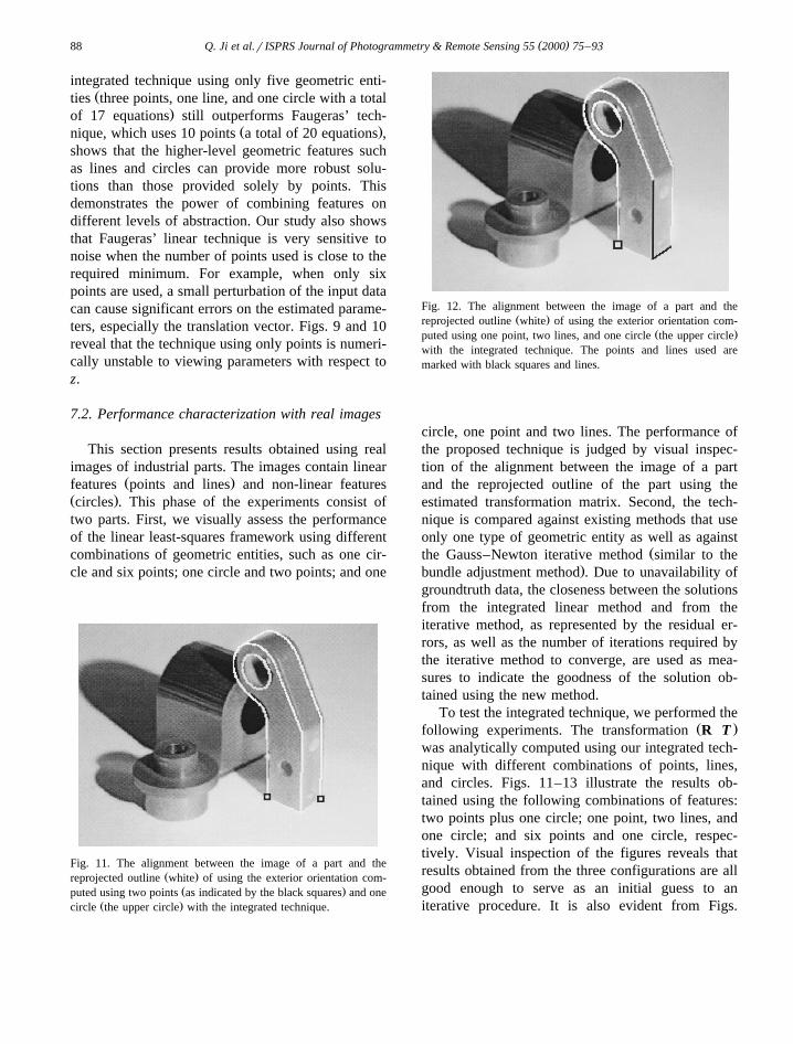
Fig. 11. The alignment between the image of a part and theŽ .reprojected outline white of using the exterior orientation com-
Ž .puted using two points as indicated by the black squares and oneŽ .circle the upper circle with the integrated technique.
Fig. 12. The alignment between the image of a part and theŽ .reprojected outline white of using the exterior orientation com-
Ž .puted using one point, two lines, and one circle the upper circlewith the integrated technique. The points and lines used aremarked with black squares and lines.
circle, one point and two lines. The performance ofthe proposed technique is judged by visual inspec-tion of the alignment between the image of a partand the reprojected outline of the part using theestimated transformation matrix. Second, the tech-nique is compared against existing methods that useonly one type of geometric entity as well as against
Žthe Gauss–Newton iterative method similar to the.bundle adjustment method . Due to unavailability of
groundtruth data, the closeness between the solutionsfrom the integrated linear method and from theiterative method, as represented by the residual er-rors, as well as the number of iterations required bythe iterative method to converge, are used as mea-sures to indicate the goodness of the solution ob-tained using the new method.
To test the integrated technique, we performed theŽ .following experiments. The transformation R T
was analytically computed using our integrated tech-nique with different combinations of points, lines,and circles. Figs. 11–13 illustrate the results ob-tained using the following combinations of features:two points plus one circle; one point, two lines, andone circle; and six points and one circle, respec-tively. Visual inspection of the figures reveals thatresults obtained from the three configurations are allgood enough to serve as an initial guess to aniterative procedure. It is also evident from Figs.
( )Q. Ji et al.r ISPRS Journal of Photogrammetry & Remote Sensing 55 2000 75–93 89
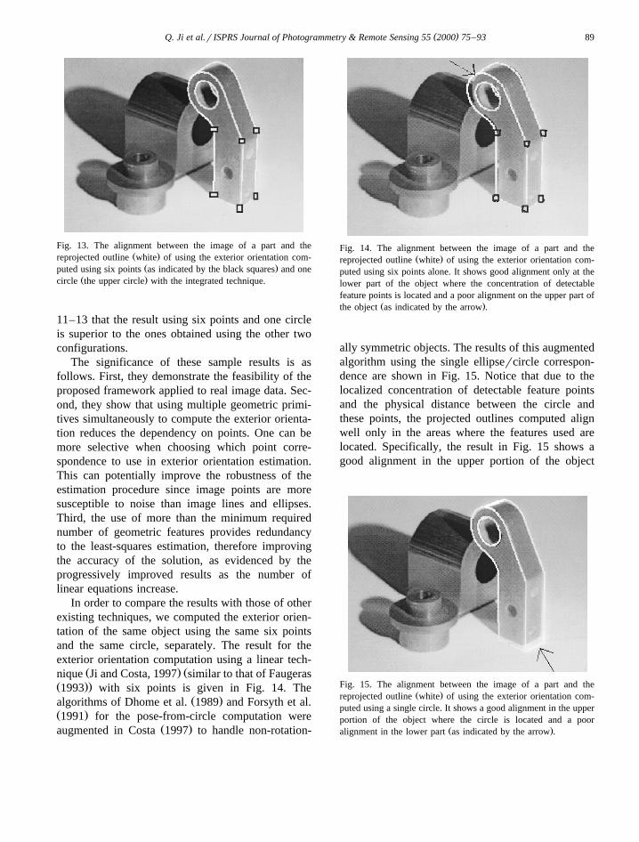
Fig. 13. The alignment between the image of a part and theŽ .reprojected outline white of using the exterior orientation com-
Ž .puted using six points as indicated by the black squares and oneŽ .circle the upper circle with the integrated technique.
11–13 that the result using six points and one circleis superior to the ones obtained using the other twoconfigurations.
The significance of these sample results is asfollows. First, they demonstrate the feasibility of theproposed framework applied to real image data. Sec-ond, they show that using multiple geometric primi-tives simultaneously to compute the exterior orienta-tion reduces the dependency on points. One can bemore selective when choosing which point corre-spondence to use in exterior orientation estimation.This can potentially improve the robustness of theestimation procedure since image points are moresusceptible to noise than image lines and ellipses.Third, the use of more than the minimum requirednumber of geometric features provides redundancyto the least-squares estimation, therefore improvingthe accuracy of the solution, as evidenced by theprogressively improved results as the number oflinear equations increase.
In order to compare the results with those of otherexisting techniques, we computed the exterior orien-tation of the same object using the same six pointsand the same circle, separately. The result for theexterior orientation computation using a linear tech-
Ž . Žnique Ji and Costa, 1997 similar to that of FaugerasŽ ..1993 with six points is given in Fig. 14. The
Ž .algorithms of Dhome et al. 1989 and Forsyth et al.Ž .1991 for the pose-from-circle computation were
Ž .augmented in Costa 1997 to handle non-rotation-
Fig. 14. The alignment between the image of a part and theŽ .reprojected outline white of using the exterior orientation com-
puted using six points alone. It shows good alignment only at thelower part of the object where the concentration of detectablefeature points is located and a poor alignment on the upper part of
Ž .the object as indicated by the arrow .
ally symmetric objects. The results of this augmentedalgorithm using the single ellipsercircle correspon-dence are shown in Fig. 15. Notice that due to thelocalized concentration of detectable feature pointsand the physical distance between the circle andthese points, the projected outlines computed alignwell only in the areas where the features used arelocated. Specifically, the result in Fig. 15 shows agood alignment in the upper portion of the object
Fig. 15. The alignment between the image of a part and theŽ .reprojected outline white of using the exterior orientation com-
puted using a single circle. It shows a good alignment in the upperportion of the object where the circle is located and a poor
Ž .alignment in the lower part as indicated by the arrow .

( )Q. Ji et al.r ISPRS Journal of Photogrammetry & Remote Sensing 55 2000 75–9390
Table 1Exterior orientations from different methods
Ž .Method R T mm
0.410 y0.129 y0.902Ž . w xPoint only Fig. 14 y43.125 y25.511 1232.0360.606 y0.700 0.376
y0.681 y0.701 y0.208
0.302 0.302 y0.932Ž . w xCircle only Fig. 15 y35.161 y15.358 1195.2930.692 y0.628 0.355
y0.655 y0.753 y0.054
0.398 y0.142 y0.902Ž . w xPoints and circle Fig. 13 y43.077 y26.400 1217.8550.554 y0.667 0.336
y0.700 y0.684 y0.201
0.341 y0.156 y0.927Ž . w xBundle adjustment Fig. 16 y43.23 y28.254 1273.070.631 y0.693 0.349
y0.697 y0.704 y0.137
where the circle is located and a poor alignment inŽ .the lower part as indicated by the arrow . On the
other hand, the result in Fig. 14 shows a goodalignment only at the lower part of the object wherethe concentration of detectable feature points is lo-cated and a poor alignment on the upper part of the
Ž .object as indicated by the arrow .Visual inspection of the results in Figs. 13–15
shows the benefits of the new technique over theexisting methods. The model reprojection using thetransformation matrix obtained using the new tech-nique yields a better alignment than those using onlypoints or only ellipsercircle correspondences. Tocompare the performance quantitatively, we comparethe transformation matrices obtained using the three
Ž .methods with different combinations of featuresagainst the one obtained from the iterative procedureŽ .bundle adjustment Table 1 shows the numericalresults for the transformations obtained from usingonly points, only the circle, and a combination ofpoints and circle. The results from each method were
Table 2Iterations needed for the bundle adjustment method to convergeusing the solutions of the three linear methods as initial estimates
Method Number of iterations
Points only 4Circle only 6Points and circle 1
then used as the initial guess to the iterative Gauss–Newton method. The final transformation obtainedafter the convergence of the iterative method isshown in the last row of Table 1. These final resultsare the same regardless of which initial guess wasused. But they vary in number of iterations requiredas shown in Table 2.
Table 2 summarizes the number of iterations re-quired for the iterative procedure to converge usingas initial guesses the results from the three linearmethods mentioned in Table 1. Fig. 16 shows theresults from the iterative procedure.
Fig. 16. The result obtained from the bundle adjustment methodafter only one iteration using the solution in Fig. 13 as approxima-tion.

( )Q. Ji et al.r ISPRS Journal of Photogrammetry & Remote Sensing 55 2000 75–93 91
It is evident from Tables 1 and 2 and Fig. 16 thatthe new technique yields a transformation matrix thatis closer to the one obtained from the bundle adjust-ment procedure and therefore requires fewer itera-
Ž .tions one here for the bundle adjustment method toconverge. By contrast, the final results for initialguesses obtained using only points and only onecircle require four and six iterations, respectively, forthe bundle adjustment procedure to converge. Theresult from the quantitative study echoes the conclu-sion from visual inspection: the new technique offersbetter estimation accuracy, because it is capable offusing all information available.
To further validate our technique, we tested it onover 50 real images with similar results. Fig. 17 giveresults of applying the integrated technique to differ-ent industrial parts with different combinations ofgeometric features. Our experiments also reveal, aswas theoretically expected for a system of linearequations of the form AXsb, a decay in robustnesswhen the number of equations in the linear systemreaches the minimum required for a solution to befound. The premise is that one should make use of asmany available features as possible in order to im-
Fig. 17. Results of the integrated method applied to differentindustrial parts.
prove accuracy and robustness. Our technique fol-lows this principle.
8. Discussion and summary
In this paper, we presented a linear solution to theexterior orientation estimation problem. The maincontributions of this research are the linear frame-work for fusing information available from differentgeometric entities and for introducing a novel tech-nique that approximately imposes the orthonormalityconstraints on the rotation matrix sought. Experimen-tal evaluation using both synthetic data and realimages show the effectiveness of our technique forimposing orthonormal constraints in improving esti-mation errors. The technique is especially effectivewhen the SNR is low or fewer geometric entities areused. The performance study also revealed superior-ity of the integrated technique to a competing lineartechnique using only points in terms of robustnessand accuracy.
We want to discuss several issues related to theproposed algorithm. First, the algorithm is designedfor single images. It can be easily extended to multi-ple images by cascading the least-squares frameworkfor each image. Second, it is worth to point out thatthe final accuracy of the estimated exterior orienta-tion depends not only on the measurement accuracy,the feature number, but also heavily on distributionof measurements. In the work described in this pa-per, we did not address this issue. This will be afuture task. Thirdly, the paper emphasizes only thefact that we introduce a framework that is CAPA-BLE of integrating different types of geometric fea-tures for estimating exterior camera parameters.Studying the effects of what actually cause thisimprovement is an interesting and nontrivial task.We will leave it for future study. Fourthly, whencomparing with point-only method with the inte-grated approach, we used only 10 points. In practice,many more points may be used for the points-onlymethod. This can significantly improve the perfor-mance of the point-only methods and therefore re-duce the performance difference between the two.Finally, for the integrated approach, we assume equalweighting for different features. As part of futurework, we plan to use error propagation to compute a

( )Q. Ji et al.r ISPRS Journal of Photogrammetry & Remote Sensing 55 2000 75–9392
covariance matrix for each type of feature. Thecovariance matrices can then used as weightings fordifferent features.
The new technique proposed in this paper is idealfor applications such as industrial automation whererobustness, accuracy, computational efficiency, andspeed are needed. Its results can also be used asinitial estimates in certain applications where moreaccurate camera parameters are needed. The pro-posed algorithm is more suitable for images withman-made objects, especially in close-range applica-tions.
References
Abdel-Aziz, Y.I., Karara, H.M., 1971. Direct linear transformationfrom comparator co-ordinates into object–space coordinates.ASP Symp. on Close-Range Photogrammetry, 1–18.
Abidi, M.A., 1995. A new efficient and direct solution for poseestimation using quadrangular targets — algorithm and evalu-
Ž .ation. IEEE T-PAMI 17 5 , 534–538.Bopp, H., Krauss, H., 1978. An orientation and calibration method
for non-topographic applications. Photogramm. Eng. RemoteŽ .Sens. 44 9 , 1191–1196.
Chen, S.-Y., Tsai, W.-H., 1990. Systematic approach to analyticdetermination of camera parameters by line features. Pattern
Ž .Recognit. 23 8 , 859–897.Chen, S.Y., Tsai, W.H., 1991. Determination of robot locations by
common object shapes. IEEE Trans. Robotics Automation 7Ž .1 , 149–156.
Costa, M.S., 1997. Object recognition and pose estimation usingappearance-based features and relational indexing. PhD Dis-sertation, Intelligent Systems Laboratory, Department of Elec-trical Engineering, University of Washington, Seattle.
Dhome, M.D., Lapreste, J.T., Rives, G., Richetin, M., 1989.Spatial localization of modeled objects of revolution inmonocular perspective vision. First European Conference onComputer Vision, 475–485.
Doehler, M., 1975. In: Verwendung von pass-linien anstelle vonpass-punkten in der nahbildmessung Festschrift K. Schwidef-sky, Institute for Photogrammetry and Topography, Univ. ofKarlsruhe, Germany, pp. 39–45.
Drewniok, C., Rohr, K., 1997. Exterior orientation — an auto-matic approach based on fitting analytic landmark models.
Ž .ISPRS J. Photogramm. Remote Sens. 52 3 , 132–145.Echigo, T., 1990. Camera calibration technique using three sets of
Ž .parallel lines. Mach. Vision Appl. 3 3 , 159–167.Ethrog, U., 1984. Non-metric camera calibration and photo orien-
tation using parallel and perpendicular lines of photographedŽ .objects. Photogrammetria 39 1 , 13–22.
Faugeras, O.D., 1993. Three Dimensional Computer Vision: aGeometric Viewpoint. MIT Press.
Finsterwalder, R., 1991. Zur verwendung von passlinien bei pho-Ž .togrammetrischen aufgaben. Z. Vermessungswesen 116 2 ,
60–66.Fischler, M.A., Bolles, R.C., 1981. Random sample consensus: a
paradigm for model fitting with applications to image analysisŽ .and automated cartography. Communications ACM 24 6 ,
381–395.Forkert, G., 1996. Image orientation exclusively based on free-
form tie curves. Int. Arch. Photogramm. Remote Sens. 31Ž .B3 , 196–201.
Forsyth, D., Mundy, J.L., Zisserman, A., Corlho, C., Heller, A.,Rothwell, C., 1991. Invariant descriptors for 3d object recogni-tion and pose. IEEE Trans. PatternAnalysis Machine Intelli-
Ž .gence 13 10 , 971–991.Gao, M., 1992. Estimating camera parameters from projection of a
rectangular parallelepiped. J. Northwest. Polytechnic Univ. 10Ž .4 , 427–433.
Haralick, R.M., 1988. Determining camera parameters from theŽ .perspective projection of rectangle. Pattern Recognit. 22 3 ,
225–230.Haralick, R.M., Chu, Y.H., 1984. Solving camera parameters from
perspective projection of a parameterized curve. PatternŽ .Recognit. 17 6 , 637–645.
Haralick, R.M., Shapiro, L.G., 1993. In: Computer and RobotVision vol. 2 Addison-Wesley, Reading, MA.
Haralick, R.M., Joo, H., Lee, C., Zhang, X., Vaidya, V., Kim, M.,1989. Pose estimation from corresponding point data. IEEE
Ž .Trans. Systems, Man Cybernetics 19 6 , 1426–1446.Haralick, R.M., Lee, C., Ottenberg, K., Nolle, M., 1994. Review
and analysis of solutions of the three point perspective poseŽ .estimation. Int. J. Comput. Vision 13 3 , 331–356.
Heikkila, J., 1990. Update calibration of a photogrammetric sta-Ž .tion. Int. Arch. Photogramm. Remote Sens. 28 5r2 , 1234–
1241.Heikkila, J., 1991. Use of linear features in digital photogramme-
Ž .try. Photogramm. J. Finland 12 2 , 40–56.Holt, R.J., Netravali, A.N., 1991. Camera calibration problem:
some new results. Comput. Vision, Graphics Image ProcessingŽ .54 3 , 368–383.
Horn, B.K.P., 1987. Closed-form solution of absolute orientationŽ .using quaternions. J. Opt. Soc. Am. A 4 4 , 629–642.
Hung, Y., Yeh, P.S., Harwood, D., 1985. Passive ranging toknown planar point sets. Proc. IEEE Int. Conf. RoboticsAutomation, 80–85.
Ji, Q., Costa, M.S., 1997. New linear techniques for pose estima-tion using point correspondences. Intelligent Systems Lab.,Department of Electrical Engineering University of Washing-ton, Technical Report aISL-04-97.
Kager, H., 1989. A universal photogrammetric adjustment system.Opt. 3D Meas., 447–455.
Kamgar-Parsi, B., Eas, R.D., 1990. Calibration of stereo systemwith small relative angles. Comput. Vision, Graphics Image
Ž .Processing 51 1 , 1–19.Kruck, E., 1984. A program for bundle adjustment for engineering
applications — possibilities, facilities and practical results.Ž .Int. Arch. Photogramm. Remote Sens. 25 A5 , 471–480.
Kumar, R., Hanson, A.R., 1989. Robust estimation of camera

( )Q. Ji et al.r ISPRS Journal of Photogrammetry & Remote Sensing 55 2000 75–93 93
location and orientation from noisy data having outliers. IEEEWorkshop on Interpretation of 3D Scenes, 52–60.
Lee, R., Lu, P.C., Tsai, W.H., 1990. Robot location using singleviews of rectangular shapes. Photogramm. Eng. Remote Sens.
Ž .56 2 , 231–238.Linnainmaa, S., Harwood, D., 1988. Pose determination of a
three-dimensional object using triangle pairs. IEEE T-PAMIŽ .10 11 , 634–647.
Liu, Y., Huang, T.S., Faugeras, O.D., 1990. Determination ofcamera locations from 2d to 3d line and point correspondence.
Ž .IEEE Trans. Pattern Analysis Machine Intelligence 12 1 ,28–37.
Lugnani, J.B., 1980. Using digital entities as control. PhD thesis,Department of Surveying Engineering, The University of NewBrunswick, Fredericton.
Ma, D.S., 1993. Conics-based stereo, motion estimation and poseŽ .determination. Int. J. Comput. Vision 10 1 , 7–25.
Maas, H.G., 1999. Image sequence based automatic multi-camerasystem calibration techniques. ISPRS J. Photogramm. Remote
Ž .Sens. 54 6 , 352–359.Masry, S.E., 1981. Digital mapping using entities: a new concept.
Ž .Photogramm. Eng. Remote Sens. 48 11 , 1561–1599.Mikhail, E.M., 1993. Linear features for photogrammetric restitu-
tion and other object completion. In: Proc. SPIE, 1944. pp.16–30.
Mikhail, E.M., Mulawa, D.C., 1985. Geometric form fitting inindustrial metrology using computer-assisted theodolites.ASPrACSM Fall Meeting, 1985.
Mulawa, D., 1989. Estimation and photogrammetric treatment oflinear features. PhD dissertation, School of Civil Engineering,Purdue University, West Lafayette, USA.
Mulawa, D.C., Mikhail, E.M., 1988. Photogrammetric treatmentof linear features. Int. Arch. Photogramm. Remote Sens. 27Ž .B10 , 383–393.
Okamoto, A., 1981. Orientation and construction of models: PartI. The orientation problem in close-range photogrammetry.
Ž .Photogramm. Eng. Remote Sens. 47 11 , 1615–1626.Paderes, F.C., Mikhail, E.M., Foerstner, W., 1984. Rectification
of single and multiple frames of satellite scanner imageryusing points and edges as control. In: NASA Symp. onMathematical Pattern Recognition and Image Analysis, Hous-ton.
Petsa, E., Patias, P., 1994a. Formulation and assessement of
straight line based algorithms for digital photogrammetry. Int.Ž .Arch. Photogramm. Remote Sens. 5 , 310–317.
Petsa, E., Patias, P., 1994b. Sensor attitude determination usingŽ .linear features. Int. Arch. Photogramm. Remote Sens. 30 1 ,
62–70.Pettersen, A., 1992. Metrology norway system — an on-line
industrial photogrammetric system. Int. Arch. Photogramm.Ž .Remote Sens. 29 B5 , 43–49.
Phong, T.Q., Horward, R., Yassine, A., Tao, P., 1995. Objectpose from 2-d to 3d point and line correspondences. Int. J.
Ž .Comput. Vision 15 3 , 225–243.Rothwell, C.A., Zisserman, A., Marinos, C.I., Forsyth, D., Mundy,
J.L., 1992. Relative motion and pose from arbitrary planeŽ .curves. Image and Vision Computing 10 4 , 251–262.
Shan, J., 1996. An algorithm for object reconstruction withoutinterior orientation. ISPRS J. Photogramm. Remote Sens. 51Ž .6 , 299–307.
Strunz, G., 1992. Image orientation and quality assessment infeature based photogrammetry. Robust Comput. Vision, 27–40.
Sutherland, I.E., 1974. Three-dimensional data input by tablet.Ž .Proc. IEEE 62 4 , 453–461.
Szczepanski, W., 1958. Die loesungsvorschlaege fuer den raeum-lichen rueckwaertseinschnitt. Deutsche Geodaetische Kommis-sion, Reihe C, 29.
Tommaselli, A.M.G., Lugnani, J.B., 1988. An alternative mathe-matical model to the collinearity equation using straight fea-
Ž .tures. Int. Arch. Photogramm. Remote Sens. 27 B3 , 765–774.Tommaselli, A.M.G., Tozzi, C.L., 1996. A recursive approach to
space resection using straight lines. Photogramm. Eng. RemoteŽ .Sens. 62 1 , 57–66.
Tsai, R., 1987. A versatile camera calibration technique for high-accuracy 3d machine vision metrology using off-the-shelf tv
Ž .cameras and lens. IEEE J. Robotics Automation 3 4 , 323–344.
Wang, L.L., Tsai, W.H., 1990. Computing camera parametersusing vanishing-line information from a rectangular par-allepiped. Mach. Vision Appl. 3, 129–141.
Wang, X., Xu, G., 1996. Camera parameters estimation andŽ .evaluation in active vision system. Pattern Recognit. 29 3 ,
439–447.Weng, J., Huang, T.S., Ahuja, N., 1992. Motion and structure
from line correspondences closed-form solution, uniquenessŽ .and optimization. IEEE T-PAMI 14 3 , 318–336.