A robust and efficient implicit solvation model

for fast semiempirical methods

Sebastian Ehlert, Marcel Stahn, Sebastian Spicher, and Stefan Grimme∗

Mulliken Center of Theoretical Chemistry, Bonn, Germany

E-mail: grimme@thch.uni-bonn.de

Abstract

We present a robust and efficient method to implicitly account for solvation ef-

fects in modern semiempirical quantum mechanics and force-fields. A computation-

ally efficient yet accurate solvation model based on the analytical linearized Poisson–

Boltzmann (ALPB) model is parameterized for the extended tight binding (xTB) and

density functional tight binding (DFTB) methods as well as for the recently proposed

GFN-FF general force-field. The proposed methods perform well over a broad range

of systems and applications, from conformational energies over transition-metal com-

plexes to large supramolecular association reactions of charged species. For hydra-

tion free energies of small molecules GFN1-xTB(ALPB) is reaching the accuracy of

sophisticated explicitly solvated approaches, with a mean absolute deviation of only

1.4 kcal/mol compared to experiment. Logarithmic octanol–water partition coefficients

(logKow) are computed with a mean absolute deviation of about 0.65 using GFN2-

xTB(ALPB) compared to experimental values indicating a consistent description of

differential solvent effects. Overall, more than twenty solvents for each of the six

semiempirical methods are parameterized and tested. They are readily available in the

xtb and dftb+ programs for diverse computational applications.

1

1 Introduction

Solvation is ubiquitous in biological systems and plays an important role in many aspects of

chemistry. Therefore, any computational method targeting to describe structures or interac-

tions under realistic conditions must account for solvation effects. Solute–solvent interactions

for example in hydration processes1,2 or binding free energy computation3 can be evaluated

explicitly by free energy methods like thermodynamic integration4–6 or free energy pertur-

bation.7–10 Techniques like metadynamics,11 umbrella sampling12 or replica exchange13,14

allow to enhance the efficiency of the configuration space sampling determining the preci-

sion in the free energy computation.15 Beside molecular dynamic based sampling techniques,

Monte-Carlo methods can be used to effectively sample the conformational landscape.1,16,17

While those methods are a suitable for accurate free energy computation, they require sig-

nificant computational effort, which can be prohibitive for detailed investigations of chemical

reaction mechanisms or high throughput computational workflows.

A practical compromise is usually found in the application of implicit solvation mod-

els.18–24 In this approach, the contributions to the solvation free energy are often partitioned

into polar (electrostatic) and non-polar (dispersion and cavity) solvation free energies, which

allows devising tailored models for each contribution separately. The polar contribution

is mostly approximated by conductor-like screening (COSMO)25 or polarizable continuum

models (PCM).26–29 Implicit solvation models like the conductor-like screening model for real

solvents (COSMO-RS),24,30–32 the solvent models based on solute electron density (SMD)33

or the three-dimensional reference interaction side model (3D-RISM)34–36 enable accurate

computation of solvation free energies based on standard (mostly DFT) electronic structure

input data. However, while low-scaling implementations of COSMO/PCM have been pro-

posed,37 they still yield a noticeable computational overhead for force-field (FF) or semiem-

pirical quantum mechanical (SQM) methods. For example the PM6 and PM7 methods

have been successfully combined with COSMO38,39 in previous studies using linear scaling

algorithms.

2

A promising alternative are generalized Born (GB) models,40–42 which are used in the

reaction field based solvation models (SM), like SM6,43 SM844,45 or SM1246 and for FFs as

generalized Born and surface area model (GBSA).47–49 These models allow devising com-

putationally efficient but yet accurate schemes to include solvation effects in large scale

simulations.50

For the many SQM methods available, robust solvation models are needed, as this is

tightly bound to the applicability of the respective methods in computational chemistry or

biology.51,52 One of the most promising members of the family of SQM methods are tight

binding (TB) approaches, like density functional tight binding (DFTB)53,54 or extended

tight binding (xTB).55 While the xTB methods were from the very beginning coupled with

an implicit solvation model,56,57 only a few DFTB implementations account for solvation

effects.58–60

In this work we revisit the implicit solvation models tied with the xTB methods and try

to systematically improve the underlying theory as well as the parametrization. Both exper-

imental data from the MNSOL database43,61,62 and theoretical values based on COSMO-RS

are used as reference data in the fit. To allow for a fair comparison with DFTB, we also

implemented, parameterized, and tested the implicit solvation models developed for xTB

with three DFTB Hamiltonians. Furthermore, we include the recently devised general force

field GFN-FF63 which is not equipped with a tailored solvation model yet, but employed the

GFN2-xTB solvation model in Ref. 63.

We investigate the accuracy of solvation free energies using the implicit solvation models

based on the curated FreeSolv database64,65 for experimental hydration free energies. Since

accurate experimental data are usually only available for small compounds, we devise a

benchmark set of back-corrected experimental association solvation free energies for large

supramolecular complexes as well, building upon the established S30L set.66 Furthermore, we

employ a set of experimental octanol–water partition coefficients for 26 organic compounds

and investigate the differential description of two solvents by the new models.

3

This paper is organized as follows. In section 2 the theory and algorithms used to imple-

ment the models with the TB methods are presented. Technical details of the parametriza-

tion and generation of reference data are described in section 3. In section 4 performance

comparisons for a wide range of systems and benchmarks of the investigated methods are

shown. Finally, in section 5 conclusions and perspectives are presented.

2 Theory

To describe a solute in a given solvent or dielectric medium the solvation free energy ∆Gsolv

is partitioned into a polar contribution ∆Gpolar, which depends on the electrostatic potential,

a non-polar contribution ∆Gnpol, which depends on the shape of the solute cavity and a con-

stant shift ∆Gshift depending on the reference state for the solvation process. The solvation

free energy is therefore given as

∆Gsolv = ∆Gpolar + ∆Gnpol + ∆Gshift. (1)

This partitioning is commonly used in many popular solvation models like GBSA42,50

or SMD33 resulting in energy expressions of different complexity for the individual con-

tributions. Changes in the internal free energy of the molecule (rotation, vibration and

conformational partition function) upon solvation is mostly not accounted for explicitly but

absorbed into the empirical parameters of the model (see section 4.1).

A suitable form for an efficient evaluation of the polar contributions is the analytical

linearized Poisson–Boltzmann (ALPB) model.,48 where the polar contribution is given by

∆GALPBpolar = −1

2

(1

εin− 1

εout

)1

1 + αβ

N∑A=1

N∑B=1

qAqB

(1

f(RAB, aA, aB)+

αβ

Adet

), (2)

and εin is the dielectric constant of the solute, εout the dielectric constant of the solvent, qA/B

are atomic partial charges, f is the interaction kernel, aA/B are the atomic Born radii for

4

atoms A and B and Adet is the electrostatic size of the solute. The value of α is fixed at

0.571214 following the work of Sigalov et al.48 and β is εin/εout. The electrostatic size Adet is

calculated from the inertia tensor as proposed in Ref. 48, while for εin the dielectric constant

of the vacuum, i. e., one, is chosen. Since GB models are derived in the limit of εout →∞ or

β → 0 we can effectively cast them into the same energy expression as the ALPB model by

setting αβ to zero.

In this work we will test two different interaction kernels, first the canonical interaction

kernel proposed by Still42

fStillAB =

(R2

AB + aAaB exp

[− R2

AB

4aAaB

]) 12

(3)

and the more recently proposed P16 kernel49

fP16AB = RAB +

√aAaB

(1 +

1.028 ·RAB

16√aAaB

)16

. (4)

The evaluation of the interaction kernel requires the atomic Born radii aA/B, which are

obtained by carrying out an integral over the molecular volume of the solute. For computa-

tional efficiency, we employ a pairwise approximate scheme, namely the Onufriev–Bashford–

Case (OBC) corrected integrator termed GBOBCII.47 The Born radius in this integrator is

calculated by

1

aA

=1

ascale

(1

RvdwA −Roffset

− tanh[bΨA − cΨ2A + dΨ3

A]

RvdwA

), (5)

where RvdwA are the D3 van-der-Waals radii,67 ascale is a global scaling parameter for the Born

radii, Roffset is a global shift parameter to introduce more flexibility for the van-der-Waals

radii and ΨA is the pairwise approximation to the integral over the molecular volume given

by

ΨA =Rvdw

A −Roffset

2

N∑B 6=A

Ω(RAB, RvdwA , sB ·Rvdw

B ), (6)

5

where Ω is the pairwise contribution to the approximate volume. To compensate for the

overestimation of the molecular volume in Ω, an element-specific de-screening parameter sB

is introduced for the van-der-Waals radius of the other atoms.

2.1 Non-polar Surface Area Contribution

To account for non-polar contributions to the solvation free energy we include a surface

area (SA) model using the solvent-accessible surface area (SASA) to compute the free en-

ergy needed to form the solute–solvent cavity and to account for solute–solvent dispersion

interactions by

∆GSAnpol =

N∑A

γAσA, (7)

where γA is the surface tension of each atom and σA is its SASA. The surface tension is fitted

as an element-specific parameter. To evaluate the complete SASA of the molecule we use

σtotal =

∫V

∣∣∣∣∇(∏A

HA(|~RA − ~r|))∣∣∣∣d3~r, (8)

where HA(|~RA − ~r|) is the atomic volume exclusion function,68 given by

HA(r) =

0, if r ≤ Rsurf

A − w

12

+ 34w

(r −RsurfA )− 1

4w3 (r −RsurfA )3, if Rsurf

A − w < r < RsurfA + w

1, if RsurfA + w ≤ r

(9)

The extent of the boundary region is defined by the smoothing parameter w and equals

0.3A in the here presented method. The RsurfA are the combined van-der-Waals radii Rvdw

A

with the solvent probe radius Rprobe, the latter being a global parameter.

Since the volume exclusion function and its gradient are constant everywhere except for

a narrow region around the surface area, we discretize the integral in Eq. 8 on an angular

6

Lebedev–Laikov grid69 for an efficient numerical implementation on a sparse surface grid, as

σA = 4π

Nang∑g

wgwA

N∏B 6=A

HB(RBg), (10)

where wg and wA are the angular and radial integration weights, respectively.

2.2 Hydrogen Bonding Correction

Specific interactions due to the molecular structure of the solvent, like hydrogen bonding

(HB) between the solute and solvent molecules are not accounted for due to the implicit

description of the solvent as a dielectric medium. We partition this important interaction

component in atom-resolved contributions by

∆GHBpolar =

N∑A

∆GHBA . (11)

To approximate the HB interaction we use the Keesom interaction70 of hydrogen-acceptor

and donor dipoles, µAH, and µD, respectively, with an average distance R, which is similar

to the distance of the first solvation shell. The final interaction term includes the proba-

bility δρHBsolv that a solvent molecule interaction site is close to the respective atom. This

contribution is proportional to the SASA of the interacting atom and therefore, we param-

eterize the HB contribution as

∆GHBA = −2

3

µ2AHµ

2D

ε2outkBTR6δρHB

solv ≈ −gHBA q2

A

σA

4π(RsurfA )2

, (12)

where gHBA is the HB strength, absorbing most of the constants, which is used as an element-

specific parameter. Since not all methods have the dipole moment readily available we resort

to approximate the quadratic dipole moment by the quadratic site atomic charge instead.

Using this formula allows us to include the HB contribution with the polar electrostatic

energy as a potential in the Hamiltonian or Lagrangian when minimizing the electrostatic

7

energy with no additional cost as we can reuse the already calculated SASA from the non-

polar solvation free energy.

3 Computational Details

All DFT calculations were conducted with the Turbomole 7.5.171 software package. COSMO-

RS calculations were done with COSMOtherm 1924,31,32 using the BP8672/def-TZVPD73

default level of theory. We employ the 2015, 2016, 2017, 2018 and 2019 versions of the

BP86/def-TZVP and BP86/def-TZVPD fine parametrization in this work. The presented

solvation models were implemented in the open source software packages xtb55,74 and DFTB+54?

and subsequently released with xtb version 6.3.2 and DFTB+ version 20.1, which were

used to conduct all xTB and DFTB calculations, respectively. For the third-order variant

of DFTB, the 3ob parametrization is employed75–78 and the mio parametrization is used

for the second-order DFTB variant.79–81 The ob2-base parametrization is used for the LC-

DFTB Hamiltonian.82 All DFTB Hamiltonians are combined with the D4(EEQ) London

dispersion model without three-body contributions83 using the parameters published in Ref.

54. Conformational searches and analysis were conducted with the conformer–rotamer en-

semble search tool (CREST) version 2.10 using the iMTD-GC algorithm.84,85 For high-level

reference calculations the CRENSO workflow version 1.0.0 was used.86–88

3.1 ALPB Training Set

The training set for the ALPB Solvation model consists of a mixture of experimental and

theoretical solvation free energies. For the experimental part, we chose the Minnesota Sol-

vation Database (MNSOL) version 201243,61,62 to serve as reference data. This database

includes two types of solvation free energies: absolute solvation free energies and relative

solvation free energies between various organic solvents and water. For the parametrization

of ALPB, only the absolute solvation free energies were taken. In total the MNSOL Database

8

consists of experimental solvation free energies and optimized geometries for 520 neutral and

ionic solutes, including the elements H, C, N, O, F, Si, P, S, Cl, Br, and I. The contained

compounds range from small to medium sized organic solutes with a maximum atom count

of 46, as well as 31 clustered ions containing a single water molecule. These experimental

values were used for the parametrization of the solvents hexadecane, octanol, and water for

the mentioned elements, as well as the global empirical parameters in the ALPB model.

Finding sufficient experimental solvation free energies for other elements of the periodic

table and other solvents proved to be difficult. For this reason, additionally to the compounds

in the MNSOL Database, we used the fit set created for the parametrization of the xTB

Hamiltonians as it covers a wide range of elements.56,57 In total the set used here contains

about 2500 compounds for 67 elements. The geometries were optimized with the functional

PBEh-3c.89 The δGsolv reference values were obtained using COSMO-RS with the default

version 2016 parametrization.24,31,32

3.2 Parametrization

Other than the physical constants ε, m, and φ, which describe the dielectric constant, the

mass and the mass density of the solvent, ALPB uses two types of parameters: global

parameters and element specific parameters. The global parameters are Gshift in equation

1, αscale and Roffset in equation 5 and the probe radius RProbe, which is included in RsurfA

in equation 10. The element specific parameters are sX in equation 6, γA in equation 7 and

gHBA in equation 12. The parameterized solvents are shown in Tab. 1. The ALPB solvation

model employs the P16 interaction kernel, while we use the Still interaction kernel for the

GBSA solvation model in this work.

For the parameter fit, a fully automated workflow was implemented. Therefore, the com-

pounds of the ALPB test set were split into several subgroups, depending on the contained

elements. The reference solvation free energies (MNSOL database or COSMO-RS) refer to

the process of transferring the molecule from the gas phase to the liquid phase, and hence,

9

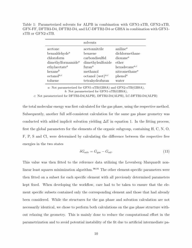
Table 1: Parameterized solvents for ALPB in combination with GFN1-xTB, GFN2-xTB,GFN-FF, DFTB3-D4, DFTB2-D4, and LC-DFTB2-D4 or GBSA in combination with GFN1-xTB or GFN2-xTB.

solvents

acetone acetonnitrile anilinea

benzaldehydea benzene dichlormethanechloroform carbondisulfid dioxanea

dimethylformamidea dimethylsulfoxide etherethylacetatea furana hexadecanea,c

hexaneb methanol nitromethanea

octanola,c octanol (wet)a,c phenola

toluene tetrahydrofuran water

a: Not parameterized for GFN1-xTB(GBSA) and GFN2-xTB(GBSA),b: Not parameterized for GFN1-xTB(GBSA),

c: Not parameterized for DFTB3-D4(ALPB), DFTB2-D4(ALPB), LC-DFTB2-D4(ALPB)

the total molecular energy was first calculated for the gas phase, using the respective method.

Subsequently, another full self-consistent calculation for the same gas phase geometry was

conducted with added implicit solvation yielding ∆E in equation 1. In the fitting process,

first the global parameters for the elements of the organic subgroup, containing H, C, N, O,

F, P, S and Cl, were determined by calculating the difference between the respective free

energies in the two states

δGsolv = Ggas −Gsol. (13)

This value was then fitted to the reference data utilizing the Levenberg–Marquardt non-

linear least squares minimization algorithm.90,91 The other element-specific parameters were

then fitted on a subset for each specific element with all previously determined parameters

kept fixed. When developing the workflow, care had to be taken to ensure that the ele-

ment specific subsets contained only the corresponding element and those that had already

been considered. While the structures for the gas phase and solvation calculation are not

necessarily identical, we chose to perform both calculations on the gas phase structure with-

out relaxing the geometry. This is mainly done to reduce the computational effort in the

parametrization and to avoid potential instability of the fit due to artificial intermediate pa-

10

rameters in the geometry relaxation with implicit solvation. The influence of the geometry

relaxation will be discussed in detail in Sec. 4.1.

4 Results

In the following sections, we discuss the performance of the here presented new ALPB

solvation models on a broad range of test sets. We also compare the parametrizations of this

work with the originally published GFN1-xTB(GBSA)56 and GFN2-xTB(GBSA)57 models,

which have been shipped with the xtb program distribution55 but were not thoroughly

benchmarked so far. As statistical measures we use the mean signed deviation (MSD), mean

absolute deviation (MAD), and the standard deviation (SD) and the error range as maximum

deviation minus minimum deviation for free (solvation)energies. While the discussion mainly

focuses on the MAD we also investigated the MSD, SD and error range for all sets and will

discuss those measures if they show deviating behavior from the trends in the MAD.

4.1 Influence of geometry relaxation

To assess the possible error of neglecting geometry relaxations we evaluate the water subset

of the MNSOL database. The hydration free energy for all systems was evaluated in three

variants of the models. First, by using the gas phase optimized geometry and ignoring geom-

etry relaxations from the implicit solvation model. Second, by relaxing the geometry with the

implicit solvation model. And third, by explicitly computing the free energy of the molecule

thermostatistically in the modified rigid rotor, harmonic oscillator (mRRHO) approxima-

tion92 with a rotor-cutoff of 50 cm−1 to account for the changes in rotational (structure) and

vibrational (frequency) contributions. This requires two full geometry optimizations and

Hessian calculations.

The results with GFN2-xTB using the parametrization for GBSA and ALPB are shown

in Tab. 2. The overall error range is at 30 kcal/mol for all compounds, while only around

11

18 kcal/mol for neutral solutes. To better interpret different error sources the set is split in

neutral solutes as well as positive and negative ions.

First, we find an overall mean MAD for the hydration free energies of 1.95 and 1.88 kcal/mol

for the GBSA and ALPB solvation model, respectively. The account for geometry relaxation

only leads to small changes in the MAD for neutral solutes, slightly deteriorating the MAD

by less than 0.1 kcal/mol for both models.

For the charged solutes we find a larger MAD in the hydration free energies of 10.05 and

7.06 kcal/mol for GBSA and ALPB solvation models, respectively. While GBSA and ALPB

show similar performance for neutral solutes, ALPB represents a significant improvement for

the charged solutes due to additional charge dependent terms which are absent in GBSA.

A notable observation is that GFN2-xTB(ALPB) reduces the MAD of the hydration free

energies by half for cationic solutes compared to GFN2-xTB(GBSA). Furthermore, we find

an overall improvement of the hydration free energies when geometry relaxations are included

for charged solutes by approximately 0.2 kcal/mol for both models.

Including rotational and vibrational contributions deteriorates the performance for hydra-

tion free energies slightly but consistently for both neutral and charged solutes. Tentatively,

this slightly diminished accuracy can be attributed to the translational and rotational par-

tition functions of the ideal gas and the rigid rotor which are more approximate for the

solvated system. Approaches like a harmonic solvation model93 or heuristic corrections to

the partition function94 could improve the description but are beyond the scope of this work.

Table 2: Mean absolute deviation in kcal/mol for the hydration free energies of GFN2-xTB(ALPB) and GFN2-xTB(GBSA) for different evaluation strategies.

GFN2-xTB(GBSA) GFN2-xTB(ALPB)subset entries SP only opt. freq. SP only opt. freq.

neutral 390 1.95 2.01 2.08 1.88 1.96 2.07positive 60 9.49 9.38 9.37 4.65 4.78 4.95negative 83 11.32 10.92 11.05 9.39 8.98 9.13all charged 143 10.05 9.78 9.84 7.06 6.85 7.02all 533 4.26 4.23 4.30 3.36 3.36 3.49

12

To further investigate the influence of geometry relaxation we select 25 neutral solutes

which show a significant change in the hydration free energy upon optimization in solution.

Notable motifs with larger geometry changes are hydroxy, amid and nitro groups as well

as sulfur or phosphorous containing groups, i. e. especially polar groups. To establish a

benchmark set we optimized all 25 compounds using r2SCAN-3c95 in the gas phase and with

DCOSMO-RS96 in water. To minimize the influence of the underlying electronic structure

methods, we compare changes in bond lengths and angles between the gas phase and solvated

structure rather than absolute bond lengths and angles. Since changes in the hydration free

energy due to geometry relaxations are smaller than 0.5 kcal/mol and the root mean square

deviation between the gas phase and the solvated structure is on average only 0.15 A, small

overall geometry changes are expected. In order to put the SQM results into some perspective

and to establish a lower error bound we compute the geometry changes in addition with

r2SCAN-3c(COSMO).

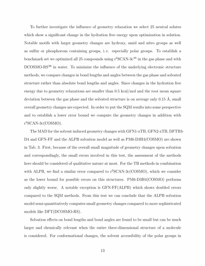
The MAD for the solvent induced geometry changes with GFN1-xTB, GFN2-xTB, DFTB3-

D4 and GFN-FF and the ALPB solvation model as well as PM6-D3H4(COSMO) are shown

in Tab. 3. First, because of the overall small magnitude of geometry changes upon solvation

and correspondingly, the small errors involved in this test, the assessment of the methods

here should be considered of qualitative nature at most. For the TB methods in combination

with ALPB, we find a similar error compared to r2SCAN-3c(COSMO), which we consider

as the lower bound for possible errors on this structures. PM6-D3H4(COSMO) performs

only slightly worse. A notable exception is GFN-FF(ALPB) which shows doubled errors

compared to the SQM methods. From this test we can conclude that the ALPB solvation

model semi-quantitatively computes small geometry changes compared to more sophisticated

models like DFT(DCOSMO-RS).

Solvation effects on bond lengths and bond angles are found to be small but can be much

larger and chemically relevant when the entire three-dimensional structure of a molecule

is considered. For conformational changes, the solvent accessibility of the polar groups in

13

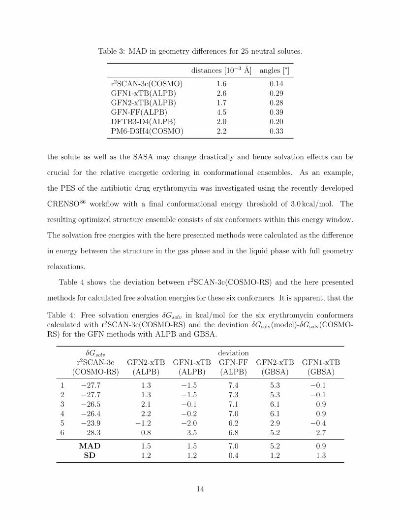
Table 3: MAD in geometry differences for 25 neutral solutes.

distances [10−3 A] angles [°]

r2SCAN-3c(COSMO) 1.6 0.14GFN1-xTB(ALPB) 2.6 0.29GFN2-xTB(ALPB) 1.7 0.28GFN-FF(ALPB) 4.5 0.39DFTB3-D4(ALPB) 2.0 0.20PM6-D3H4(COSMO) 2.2 0.33

the solute as well as the SASA may change drastically and hence solvation effects can be

crucial for the relative energetic ordering in conformational ensembles. As an example,

the PES of the antibiotic drug erythromycin was investigated using the recently developed

CRENSO86 workflow with a final conformational energy threshold of 3.0 kcal/mol. The

resulting optimized structure ensemble consists of six conformers within this energy window.

The solvation free energies with the here presented methods were calculated as the difference

in energy between the structure in the gas phase and in the liquid phase with full geometry

relaxations.

Table 4 shows the deviation between r2SCAN-3c(COSMO-RS) and the here presented

methods for calculated free solvation energies for these six conformers. It is apparent, that the

Table 4: Free solvation energies δGsolv in kcal/mol for the six erythromycin conformerscalculated with r2SCAN-3c(COSMO-RS) and the deviation δGsolv(model)-δGsolv(COSMO-RS) for the GFN methods with ALPB and GBSA.

δGsolv deviationr2SCAN-3c GFN2-xTB GFN1-xTB GFN-FF GFN2-xTB GFN1-xTB

(COSMO-RS) (ALPB) (ALPB) (ALPB) (GBSA) (GBSA)

1 −27.7 1.3 −1.5 7.4 5.3 −0.12 −27.7 1.3 −1.5 7.3 5.3 −0.13 −26.5 2.1 −0.1 7.1 6.1 0.94 −26.4 2.2 −0.2 7.0 6.1 0.95 −23.9 −1.2 −2.0 6.2 2.9 −0.46 −28.3 0.8 −3.5 6.8 5.2 −2.7

MAD 1.5 1.5 7.0 5.2 0.9SD 1.2 1.2 0.4 1.2 1.3

14

solvation free energies, as well as the deviations, significantly differ depending on the investi-

gated conformer. Note, that changes of conformational energies on the order of 1–2 kcal/mol

strongly affect thermal populations and average thermal molecular properties. With an

MAD of 1.5 kcal/mol and 1.5 kcal/mol as well as an SD of 1.2 kcal/mol, GFN2-xTB(ALPB)

and GFN1-xTB(ALPB) perform reasonably well. GFN-FF(ALPB) and GFN2-xTB(GBSA)

produce significantly too positive solvation free energies with an MAD of 7.0 kcal/mol and

5.2 kcal/mol. However, the small SD of 0.4 kcal/mol and 1.2 kcal/mol, respectively, indicates

rather systematic errors. While GFN1-xTB(GBSA) yields slightly smaller deviations than

GFN2-xTB(ALPB) and GFN1-xTB(ALPB) with an MAD of 0.9 kcal/mol, the SD is a bit

larger for the latter (1.3 kcal/mol) indicating a slightly lower robustness.

We have quantified the impact of geometry relaxations on the hydration free energies

and observed only a minor influence for small to medium sized solutes. While we can verify

that excluding geometry relaxations in the ALPB parametrization to reduce the computa-

tional effort and enhance the stability of the fit is reasonable, we also note that already

for medium-sized charged solutes, neglecting geometry relaxations can increase the error in

the calculated solvation free energies substantially. This also holds even more for solvation

effects on conformational ensembles for flexible molecules, where we refer the reader to Ref.

86 for a more detailed discussion. Thus, for general consistency we recommend to always

include geometry relaxation when calculating solvation free energies. Unless noted otherwise

all solvation free energies discussed from here on include full geometry relaxations in the

respective solvents.

4.2 Hydration Free Energies for the FreeSolv database

Water is one of the most commonly used solvents in (bio)chemistry. Yet the description of

water is difficult for implicit solvation models due to its high polarity and the importance

of HB as well as many-body (polarization) effects. To model chemistry in aqueous solution,

an accurate description of the hydration free energies is an important test. We assessed

15

the performance of the here presented methods for hydration free energies by comparing

our methods on the curated FreeSolv database, which contains currently 642 experimental

values for neutral molecules.64,65 Starting from the provided geometries the structures were

optimized with the respective methods, once with the implicit solvation model, and once in

gas phase. We also evaluated the contributions of rotational and vibrational thermostatistical

functions to the solvation energies by Hessian calculations for both, the optimized gas phase

structure, and the optimized structure in implicit solvation. Yet, only minor effects on the

overall statistics were obtained.

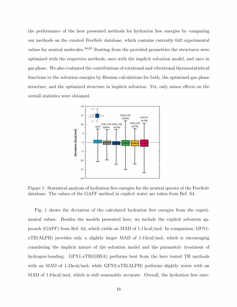
Figure 1: Statistical analysis of hydration free energies for the neutral species of the FreeSolvdatabase. The values of the GAFF method in explicit water are taken from Ref. 64.

Fig. 1 shows the deviation of the calculated hydration free energies from the experi-

mental values. Besides the models presented here, we include the explicit solvation ap-

proach (GAFF) from Ref. 64, which yields an MAD of 1.1 kcal/mol. In comparison, GFN1-

xTB(ALPB) provides only a slightly larger MAD of 1.4 kcal/mol, which is encouraging

considering the implicit nature of the solvation model and the parametric treatment of

hydrogen-bonding. GFN1-xTB(GBSA) performs best from the here tested TB methods

with an MAD of 1.3 kcal/mol, while GFN2-xTB(ALPB) performs slightly worse with an

MAD of 1.8 kcal/mol, which is still reasonably accurate. Overall, the hydration free ener-

16

gies are slightly underestimated with an MSD of −0.5 kcal/mol for GFN2-xTB(ALPB). The

GFN2-xTB(GBSA) method performs slightly worse than the ALPB variant with an MAD of

1.9 kcal/mol. The smaller standard deviation of ALPB compared to GBSA for GFN2-xTB

with 2.3 kcal/mol and 2.5 kcal/mol, respectively, indicates higher robustness and less out-

liers. DFTB(3ob)-D4(ALPB) yields an MAD of 1.7 kcal/mol and an MSD of −0.3 kcal/mol,

similar to the xTB variants.

With GFN-FF(ALPB) a respectable MAD of 2.2 kcal/mol is obtained, which is larger

than for any of the tested SQM methods but still acceptable considering the about hundred-

fold speed-up in typical applications. Evaluating the complete database with GFN-FF,

including full geometry optimizations for solution and gas phase, takes about 36 s on one

core of an Intel Xeon E5-4620 CPU, while the same calculation with GFN2-xTB takes 11 min.

4.3 Partition coefficients

An important property to characterize the distribution and accumulation of organic com-

pounds and contaminants in the environment are n-octanol/water (KOW) partition coef-

ficients, which correlate with observed biochemical and toxic effects97 and are related to

internal partitioning between biological tissues and body fluids.98 While it may be used as

a single descriptor in a linear free energy relationship (LFER), different logK relationships

are also of interest to form poly-parameter LFERs. Experimental partition coefficients for

octanol–water are mostly determined for the transition of a compound from a wet octanol

(30% water) phase to a water phase. Partition coefficients can be calculated thermody-

namically from the difference in molecular free energy between these two phases. Including

thermostatistical contributions (see Section 4.1), the value is obtained by

logKOW =1

kBT log e

(Gwater + ∆GT

mRRHO, water − (Goctanol + ∆GTmRRHO, octanol)

), (14)

17

where G is the total energy including solvation effects, GTmRRHO is the thermostatistical

contribution, kB is Boltzmann’s constant, T is the temperature, and e Euler’s number.

Figure 2: logKOW partition coefficients of 26 organic compounds ordered according to in-creasing values. The values are once calculated using wet octanol parameters and once usingdry octanol. Statistical measures are given in kcal/mol.

Fig. 2 shows calculated octanol–water partition coefficients with reference to experimental

values for 26 typical organic compounds. To classify the results, we calculated the logKOW

values with r2SCAN-3c(COSMO-RS), obtaining a very good MAD of 0.48 units. The calcu-

lations for the GFN methods were performed for dry octanol and wet octanol (30% water).

For such a complicated property, GFN2-xTB(GBSA) shows reasonably small MAD values

of 0.61 and 0.66, for dry and wet octanol, respectively. With an MAD of 0.88 and 0.67,

GFN2-xTB(ALPB) performs slightly worse than GFN1-xTB(ALPB) which is in line with

the results for the hydration free energy benchmark in section 4.2. Both methods show the

expected slight overestimation of the logKow values for dry compared to wet octanol While

not fully reaching the accuracy of the more sophisticated DFT based solvation model, given

the semi-empirical nature of the GFN methods, the results are reasonable and useful for

screening or high-throughput studies.

18

4.4 Supramolecular host–guest binding reactions

To assess the accuracy of the TB methods in combination with our parameterized solvation

models for larger systems, which are the main target application, we propose a benchmark

set of experimental, back-corrected solvation free energies for realistic host–guest binding

reactions based on the existing S30L benchmark set.66 For each of the 30 association reactions

host + guest→ guest@host an experimental binding free energy ∆Ga, exp was taken from the

original work. The reference solvation free energies ∆δGsolv are obtained according to

∆δGsolv = ∆Ga, exp −∆Ea −∆GTmRRHO, (15)

where ∆Ea are accurate DLPNO-CCSD(T) reference values from Ref. 99 and ∆GRRHO are

thermostatistical corrections taken from Ref.100 The resulting backcorrected association sol-

vation free energies range from +90 kcal/mol for [Ad2(NMe3)2@CB7]2+ (24) to −2.7 kcal/mol

for AdOH@CB7 (21). The estimated accuracy of the reference values is about 3–4 kcal/mol.

For the association reactions studied here, too strong solvation of the individual compounds

will result in a too large association solvation energy and therefore a positive MSD. Similarly,

too weak solvation of the individual compounds will result in an overall negative MSD. For

comparison, results are presented for the COSMO-RS parametrization based on BP86/def2-

TZVP densities from 2016 and the more recent 2019 parametrization for BP86/def2-TZVP

densities (for both the BP86/def2-TZVPD fine parametrization was employed for water), and

the SMD solvation model. The SMD values are based on BP86/def2-SVP calculations and

were extracted from the original S30L publication.66 The solvation free energy contribution

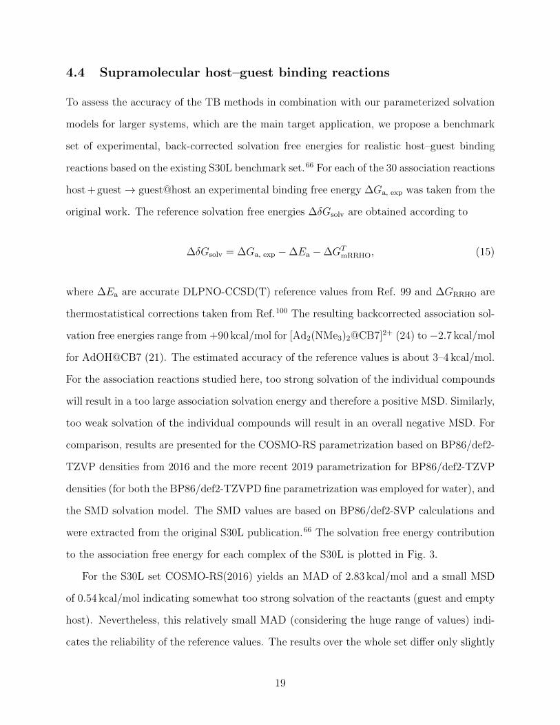
to the association free energy for each complex of the S30L is plotted in Fig. 3.

For the S30L set COSMO-RS(2016) yields an MAD of 2.83 kcal/mol and a small MSD

of 0.54 kcal/mol indicating somewhat too strong solvation of the reactants (guest and empty

host). Nevertheless, this relatively small MAD (considering the huge range of values) indi-

cates the reliability of the reference values. The results over the whole set differ only slightly

19

Figure 3: Deviation of COSMO-RS with 2016 and 2019 parametrization, GFN2-xTB withGBSA and ALPB, GFN1-xTB with GBSA and ALPB and GFN-FF(ALPB) to the back-corrected, experimental association solvation free energies. The statistical measures are givenin kcal/mol for each of the selected methods.

compared to the 2015, 2017 and 2018 parametrizations while the 2019 version in contrast

shows an increased MAD of 3.2 kcal/mol. The worse performance of the latest COSMO-

RS parametrization is mainly caused by the underestimation of the reaction solvation free

energies for water with the fine parametrization. For this variant, the MSD is shifted to

−0.1 kcal/mol. For SMD an MAD of 3.4 kcal/mol and an MSD close to zero (0.1 kcal/mol)

is obtained.

With the here presented GFN2-xTB(ALPB) solvation model a very good MAD of 5.1 kcal/mol

is achieved for an SQM method. GFN2-xTB(ALPB) slightly overestimates (MSD of 0.4 kcal/mol)

the association solvation free energy. The DFTB(3ob)-D4(ALPB) model shows a rather poor

performance with an overall MAD of 7.2 kcal/mol, which can be attributed to the poor de-

scription of the mainly dispersion bound complex 1–14, while the remaining systems are

described sufficiently well. We also evaluate the DFTB(mio)-D4(ALPB) model for the 27

systems, which can be described with the base mio-parametrization, excluding systems 4, 15

and 16 because of missing parameters for halogens. With an MAD of 7.4 kcal/mol it performs

similar to the 3ob-parametrization. Both versions significantly underestimate the values with

20

an MSD of −4.5 kcal/mol and −5.1 kcal/mol, respectively. The LC-DFTB(ob2)-D4(ALPB)

model was excluded from this test set due to missing parameters.

The GFN2-xTB(GBSA) model yields an MAD of 5.4 kcal/mol and is slightly worse com-

pared to the new GFN2-xTB(ALPB) model. The trend of overestimating the association

solvation energies is also present in the GFN2-xTB(GBSA) model as seen from the MSD of

0.8 kcal/mol. We note that GFN2-xTB(ALPB) reduces the error range significantly com-

pared to GFN2-xTB(GBSA) from 38.8 kcal/mol to only 25.3 kcal/mol.

For GFN1-xTB(GBSA) we exclude systems 15 and 16 due to missing parametrization

data for the solvent cyclohexane, for the remaining 28 systems the MAD is 6.4 kcal/mol.

GFN1-xTB(ALPB) preforms slightly better with an MAD of 6.2 kcal/mol on the 28 sys-

tems and somewhat worse with an MAD of 6.2 kcal/mol on the complete set compared to

GFN2-xTB. Both ALPB and GBSA employed together with GFN1-xTB yield a systematic

overestimation of the association solvation free energies with an MSD of 3.4 and 3.8 kcal/mol,

respectively. Again, we find that the error range with GFN1-xTB(ALPB) is significantly re-

duced compared to its GBSA variant from 60.3 to 47.1 kcal/mol. GFN-FF(ALPB) performs

with an MAD of 5.4 kcal/mol almost as good as GFN2-xTB(ALPB) on this set. Even the

error range for GFN-FF(ALPB) is similarly small with a value of 26.0 kcal/mol compared to

the SQM method.

Overall, the the ALPB solvation model together with the GFN methods yields a good

description for the solvation contributions for this challenging supramolecular reactions.

4.5 Transition Metal Chemistry

The here presented solvation models have been thoroughly investigated for neutral and

charged solutes comprised of main group elements. Here we extend the investigation to

neutral and charged solutes containing transition metal elements as well.

We evaluate all reaction solvation free energies for the reactions in the MOR41 benchmark

set101 using COSMO-RS for the three representative solvents, water, acetonitrile (ACN)

21

and tetrahydrofuran (THF). The MOR41 benchmark set consists of metal-organic reactions

featuring 3d and late transition metals and covers a wide range of possible d-block elements.

Since we are comparing with COSMO-RS, we neglect geometry relaxations consistently in

the reference method and in the tested solvation models. Due to missing parametrization

data the DFTB methods cannot be considered here.

Figure 4: Left: deviation in the MOR41 reaction solvation free energies from the COSMO-RSreference for water. Center: deviation in the MOR41 reaction solvation free energies fromthe COSMO-RS reference for acetonitrile (ACN). Right: deviation in the MOR41 reactionsolvation free energies from the DCOSMO-RS reference for tetrahydrofuran (THF). PM6-D3H4(COSMO) and PM7(COSMO) were not included in the graphic due the large errorrange of 25 and 48 kcal/mol, respectively.

The deviation of the tested methods for each of the 41 reaction solvation free energies is

shown in Fig. 4 (left panel). Overall, we find MAD values in the range of 2.3 to 3.0 kcal/mol

for the here presented solvation models. The best performing methods are GFN2-xTB, with

both ALPB and GBSA, and GFN1-xTB(GBSA) all with an MAD of 2.3 kcal/mol. Only

the ALPB solvation model for GFN1-xTB gives a slightly larger MAD of 2.5 kcal/mol. The

GFN-FF(ALPB) method yields a slightly worse MAD of 3.0 kcal/mol. For comparison we

included PM6-D3H4(COSMO) and PM7(COSMO), which perform badly for this kind of

systems with an MAD of 3.7 and 5.3 kcal/mol, respectively.

Additionally, we have investigated the same systems for ACN and THF with COSMO-RS

and the statistical data are shown in Fig. 4 (center and right panel). The overall trend of the

deviation in the reaction solvation free energies is similar compared to the reaction hydration

22

free energies, while the magnitude of the overall deviation is reduced with the polarity of the

solvent. For ACN we find an MAD ranging from 1.6 to 2.1 kcal/mol. GFN2-xTB(ALPB) is

performing best for this solvent with an MAD of 1.6 kcal/mol, while the GBSA variant yields

a larger MAD of 1.8 kcal/mol. For GFN1-xTB we find a similar good agreement using the

GBSA solvation model with an MAD of 1.7 kcal/mol and a slightly deteriorated performance

with GFN1-xTB(ALPB) (MAD 1.9 kcal/mol. PM6-D3H4(COSMO) and PM7(COSMO)

yield a rather large MAD compared to this of 3.4 and 5.1 kcal/mol. In case of THF as

solvent deviations are further reduced with MADs ranging from 1.5 to 1.8 kcal/mol for the

here presented methods.

The overall performance of the semiempirical methods is reasonable, considering that

they inherently yield a much larger error for the reaction energies, as seen in the MAD

for the MOR41 set with is 13.2 kcal/mol and 11.8 kcal/mol for GFN1-xTB and GFN2-xTB,

respectively, compared to <5 kcal/mol for well performing DFT methods.

Furthermore, we investigated the tetrakis(isonitrile)rhodium(I) cation,102 which has been

previously analyzed under different aspects in theoretical studies.83,103,104 Due to its relatively

high charge it is an interesting and challenging example for the computation of solvation free

energies. Here, we focus on the formation of the dication complex from two (mono)cations

as shown in Fig. 5.

To obtain a backcorrected reaction solvation free energy ∆δGsolv we use the DLPNO-

CCSD(T)/CBS* electronic reaction energy ∆Eelec of 8.8 kcal/mol taken from Ref. 83 and

calculate the reaction at the r2SCAN-3c level to obtain a thermostatistical correction to

the reaction free energy ∆GTmRRHO of 16.3 kcal/mol. With the experimental association

free energy ∆Ga of −2.1 kcal/mol102,104 we obtain a backcorrected reaction solvation free

energy ∆δGsolv of −27.2 kcal/mol as our benchmark value. The results are shown in Tab. 5.

For this example, clear differences are observed between the GBSA and ALPB solvation

models. In general, we find that ALPB provides generally less negative reaction solvation

free energies compared to GBSA. GFN2-xTB(ALPB) yields a reaction solvation free energy

23

Figure 5: Formation of the Rhodium dication complex. The experimental associationenergy is backcorrected using the electronic association energy ∆Eelec at the DLPNO-CCSD(T)/CBS* level of theory and thermostatistical correction to the reaction free en-ergy ∆GT

mRRHO at the r2SCAN-3c level of theory.

of −26.2 kcal/mol very close to the reference value, while GBSA is slightly over-shooting with

−29.8 kcal/mol. A similar trend between GBSA and ALPB is observed for GFN1-xTB, which

results in more positive values compared to GFN2-xTB. GFN1-xTB with GBSA solvation

model also reaches a quite good agreement of −28.3 kcal/mol, while the ALPB model is

gives an overall to positive reaction solvation free energy of −23.8 kcal/mol. We mainly

attribute this difference of 4–5 kcal/mol to the additional charge dependent contributions

in the ALPB solvation model, which are absent in most other implicit solvation models.

Table 5: Reaction solvation free energies in kcal/mol for the formation of the rhodiumdication complex.

method ∆δGsolv

reference −27.2GFN1-xTB(GBSA) −28.3GFN2-xTB(GBSA) −29.8GFN1-xTB(ALPB) −23.8GFN2-xTB(ALPB) −26.2GFN-FF(ALPB) −24.5PM6-D3H4(COSMO) −33.3PM7(COSMO) −34.0

24

Furthermore, GFN-FF(ALPB) yields a very reasonable value of −24.5 kcal/mol while PM6-

D3H4(COSMO) as well as PM7(COSMO) perform rather badly. Overall, the ALPB based

solvation models provide a decent description of the solvation effects in this challenging

transition metal reaction.

5 Conclusion

We presented a fast and computationally efficient solvation model suitable for combina-

tion with various tight binding Hamiltonians and even general force fields. A broad range

of twenty nonpolar and polar as well as protic and aprotic solvents are readily available.

In combination with the GFN family of methods all elements of the periodic table up to

Radon (Z ≤ 86) are covered. For Slater–Koster based DFTB the implicit nature of the

solvation model enables the description of systems which are unavailable with the respective

parametrizations in an explicit approach.

The resulting methods yield consistent and reasonably accurate solvation free energies

for small and large molecules with various solvents. Hydration free energies for a wide range

of solutes from the FreeSolv database are in good agreement to the experimental values

and close to the accuracy of explicitly solvated approaches which are clearly more elaborate

and computationally expensive. Additionally, the consistent description of different solvents

has been demonstrated for the accurate computation of partition coefficients, e. g., Kow for

octanol and water. For the association energies in the supramolecular S30L benchmark set,

also good results close to the backcorrected experimental values were obtained with the xTB

models.

The effect of geometry relaxations with implicit solvation models was investigated quali-

tatively and semi-quantitatively and their importance for medium-sized charged solutes was

evaluated. For properties depending on the description of a structural ensemble of flexible

solutes such as conformational free energies, the inclusion of solvation effects is indispensable.

25

The ALPB and GBSA models parameterized here are implemented in the freely available

xtb and dftb+ program packages. Based on our tests we can recommend the ALPB solvation

model in combination with GFN2-xTB as well as the GBSA solvation model in conjunction

with GFN1-xTB as routinely and consistently applicable methods for energy calculations,

geometry optimizations, molecular dynamics simulations, and vibrational frequency calcu-

lations. We are optimistic that the here presented solvation models will, together with

current and future SQM methods, be valuable in many computational chemistry studies and

workflows.

Acknowledgement

The authors thank P. Shushkov for the initial implementation of the GBSA model in xtb

and A. Hansen for proofreading the manuscript. S. E. thanks B. Hourahine for helpful

discussions and code review on the DFTB+ implementations. S. S. thanks the “Fond der

chemischen Industrie” (FCI) for financial support. This work was supported by the DFG in

the framework of the “Gottfried Wilhelm Leibniz Prize” awarded to S. G.

Supporting Information Available

The following files are available free of charge.

• LibreOffice spreadsheat containing the statistical evaluations: ESI.ods

• Tarball containing all optimized geometries: geometries.tar.xz

• Tarball containing all solvation model parameter files: parameters.tar.xz

References(1) Jorgensen, W. L.; Nguyen, T. B. Monte Carlo simulations of the hydration of substituted benzenes with OPLS potential functions. J.

Comput. Chem. 1993, 14, 195–205.

26

(2) Mobley, D. L.; Guthrie, J. P. FreeSolv: a database of experimental and calculated hydration free energies, with input files. Journal of

computer-aided molecular design 2014, 28, 711–720.

(3) Wong, C. F.; McCammon, J. A. Dynamics and design of enzymes and inhibitors. J. Am. Chem. Soc. 1986, 108, 3830–3832.

(4) Kirkwood, J. G. Statistical mechanics of fluid mixtures. J. Chem. Phys. 1935, 3, 300–313.

(5) Berens, P. H.; Mackay, D. H.; White, G. M.; Wilson, K. R. Thermodynamics and quantum corrections from molecular dynamics for liquid

water. J. Chem. Phys. 1983, 79, 2375–2389.

(6) Gilson, M. K.; Given, J. A.; Bush, B. L.; McCammon, J. A. The statistical-thermodynamic basis for computation of binding affinities: a

critical review. Biophys. J. 1997, 72, 1047–1069.

(7) Zwanzig, R. W. High-Temperature Equation of State by a Perturbation Method. I. Nonpolar Gases. The Journal of Chemical Physics 1954,

22, 1420–1426.

(8) Jorgensen, W. L.; Ravimohan, C. Monte Carlo simulation of differences in free energies of hydration. The Journal of chemical physics 1985,

83, 3050–3054.

(9) Wereszczynski, J.; McCammon, J. A. Statistical mechanics and molecular dynamics in evaluating thermodynamic properties of biomolecular

recognition. Quarterly reviews of biophysics 2012, 45, 1.

(10) Hansen, N.; Van Gunsteren, W. F. Practical aspects of free-energy calculations: a review. J. Chem. Theory Comput. 2014, 10, 2632–2647.

(11) Laio, A.; Parrinello, M. Escaping free-energy minima. Proc. Nat. Acad. Sci., USA 2002, 99, 12562–12566.

(12) Torrie, G. M.; Valleau, J. P. Nonphysical sampling distributions in Monte Carlo free-energy estimation: Umbrella sampling. Journal of

Computational Physics 1977, 23, 187–199.

(13) Hansmann, U. H. Parallel tempering algorithm for conformational studies of biological molecules. Chem. Phys. Lett. 1997, 281, 140–150.

(14) Sugita, Y.; Okamoto, Y. Replica-exchange molecular dynamics method for protein folding. Chem. Phys. Lett. 1999, 314, 141–151.

(15) Mobley, D. L.; Klimovich, P. V. Perspective: Alchemical free energy calculations for drug discovery. J. Chem. Phys. 2012, 137, 230901.

(16) Jorgensen, W. L.; Tirado-Rives, J. Molecular modeling of organic and biomolecular systems using BOSS and MCPRO. J. Comput. Chem.

2005, 26, 1689–1700.

(17) Cabeza de Vaca, I.; Qian, Y.; Vilseck, J. Z.; Tirado-Rives, J.; Jorgensen, W. L. Enhanced Monte Carlo methods for modeling proteins

including computation of absolute free energies of binding. J. Chem. Theory Comput. 2018, 14, 3279–3288.

(18) Tomasi, J.; Persico, M. Molecular interactions in solution: an overview of methods based on continuous distributions of the solvent. Chem.

Rev. 1994, 94, 2027–2094.

(19) Honig, B.; Nicholls, A. Classical electrostatics in biology and chemistry. Science 1995, 268, 1144–1149.

(20) Roux, B.; Simonson, T. Implicit solvent models. Biophysical chemistry 1999, 78, 1–20.

(21) Cramer, C. J.; Truhlar, D. G. Implicit solvation models: equilibria, structure, spectra, and dynamics. Chem. Rev. 1999, 99, 2161–2200.

(22) Orozco, M.; Luque, F. J. Theoretical methods for the description of the solvent effect in biomolecular systems. Chem. Rev. 2000, 100,

4187–4226.

(23) Tomasi, J.; Mennucci, B.; Cammi, R. Quantum mechanical continuum solvation models. Chem. Rev. 2005, 105, 2999–3094.

(24) Klamt, A. The COSMO and COSMO-RS solvation models. WIREs Comput. Mol. Sci. 2011, 1, 699–709.

(25) Klamt, A.; Schuurmann, G. COSMO: a new approach to dielectric screening in solvents with explicit expressions for the screening energy

and its gradient. Journal of the Chemical Society, Perkin Transactions 2 1993, 799–805.

27

(26) Miertus, S.; Scrocco, E.; Tomasi, J. Electrostatic interaction of a solute with a continuum. A direct utilizaion of AB initio molecular

potentials for the prevision of solvent effects. Chemical Physics 1981, 55, 117–129.

(27) Foresman, J. B.; Keith, T. A.; Wiberg, K. B.; Snoonian, J.; Frisch, M. J. Solvent effects. 5. Influence of cavity shape, truncation of

electrostatics, and electron correlation on ab initio reaction field calculations. J. Phys. C 1996, 100, 16098–16104.

(28) Barone, V.; Cossi, M. Quantum calculation of molecular energies and energy gradients in solution by a conductor solvent model. J. Phys.

Chem. A 1998, 102, 1995–2001.

(29) Cossi, M.; Rega, N.; Scalmani, G.; Barone, V. Energies, structures, and electronic properties of molecules in solution with the C-PCM

solvation model. J. Comput. Chem. 2003, 24, 669–681.

(30) Klamt, A. Conductor-like Screening Model for Real Solvents: A New Approach to the Quantitative Calculation of Solvation Phenomena. J.

Chem. Phys. 1995, 99, 2224–2235.

(31) Klamt, A.; Jonas, V.; Burger, T.; Lohrenz, J. C. W. Refinement and Parametrization of COSMO-RS. J. Phys. Chem. A 1998, 102, 5074–5085.

(32) Klamt, A. COSMO-RS : from quantum chemistry to fluid phase thermodynamics and drug design; Elsevier: Amsterdam Boston, 2005.

(33) Marenich, A. V.; Cramer, C. J.; Truhlar, D. G. Universal Solvation Model Based on Solute Electron Density and on a Continuum Model of

the Solvent Defined by the Bulk Dielectric Constant and Atomic Surface Tensions. J. Phys. Chem. B 2009, 113, 6378–6396.

(34) Ten-no, S.; Hirata, F.; Kato, S. A hybrid approach for the solvent effect on the electronic structure of a solute based on the RISM and

Hartree-Fock equations. Chemical physics letters 1993, 214, 391–396.

(35) Kovalenko, A.; Hirata, F. Three-dimensional density profiles of water in contact with a solute of arbitrary shape: a RISM approach. Chem.

Phys. Lett. 1998, 290, 237–244.

(36) Heil, J.; Kast, S. M. 3D RISM theory with fast reciprocal-space electrostatics. J. Chem. Phys. 2015, 142, 114107.

(37) Lipparini, F.; Stamm, B.; Cances, E.; Maday, Y.; Mennucci, B. Fast domain decomposition algorithm for continuum solvation models:

Energy and first derivatives. J. Chem. Theory Comput. 2013, 9, 3637–3648.

(38) Stewart, J. J. Application of the PM6 method to modeling proteins. Journal of molecular modeling 2009, 15, 765–805.

(39) Krız, K.; Rezac, J. Reparametrization of the COSMO solvent model for semiempirical methods PM6 and PM7. J. Chem. Inf. Model. 2019,

59, 229–235.

(40) Born, M. Volumen und hydratationswarme der ionen. Zeitschrift fur Physik 1920, 1, 45–48.

(41) Tucker, S. C.; Truhlar, D. G. Generalized Born fragment charge model for solvation effects as a function of reaction coordinate. Chemical

physics letters 1989, 157, 164–170.

(42) Still, W. C.; Tempczyk, A.; Hawley, R. C.; Hendrickson, T. Semianalytical treatment of solvation for molecular mechanics and dynamics.

J. Am. Chem. Soc. 1990, 112, 6127–6129.

(43) Kelly, C. P.; Cramer, C. J.; Truhlar, D. G. SM6: A density functional theory continuum solvation model for calculating aqueous solvation

free energies of neutrals, ions, and solute- water clusters. Journal of chemical theory and computation 2005, 1, 1133–1152.

(44) Marenich, A. V.; Olson, R. M.; Kelly, C. P.; Cramer, C. J.; Truhlar, D. G. Self-consistent reaction field model for aqueous and nonaqueous

solutions based on accurate polarized partial charges. Journal of Chemical Theory and Computation 2007, 3, 2011–2033.

(45) Marenich, A. V.; Cramer, C. J.; Truhlar, D. G. Universal solvation model based on the generalized born approximation with asymmetric

descreening. Journal of chemical theory and computation 2009, 5, 2447–2464.

(46) Marenich, A. V.; Cramer, C. J.; Truhlar, D. G. Generalized born solvation model SM12. Journal of Chemical Theory and Computation 2013,

9, 609–620.

28

(47) Onufriev, A.; Bashford, D.; Case, D. A. Exploring protein native states and large-scale conformational changes with a modified generalized

born model. Proteins 2004, 55, 383–394.

(48) Sigalov, G.; Fenley, A.; Onufriev, A. Analytical electrostatics for biomolecules: Beyond the generalized Born approximation. J. Chem. Phys.

2006, 124, 124902.

(49) Lange, A. W.; Herbert, J. M. Improving Generalized Born Models by Exploiting Connections to Polarizable Continuum Models. I. An

Improved Effective Coulomb Operator. J. Chem. Theory Comput. 2012, 8, 1999–2011.

(50) Onufriev, A. V.; Case, D. A. Generalized Born Implicit Solvent Models for Biomolecules. Annu. Rev. Biophys. 2019, 48, 275–296.

(51) Pecina, A.; Meier, R.; Fanfrlık, J.; Lepsık, M.; Rezac, J.; Hobza, P.; Baldauf, C. The SQM/COSMO filter: reliable native pose identification

based on the quantum-mechanical description of protein–ligand interactions and implicit COSMO solvation. Chemical Communications 2016,

52, 3312–3315.

(52) Krız, K.; Rezac, J. Benchmarking of Semiempirical Quantum-Mechanical Methods on Systems Relevant to Computer-Aided Drug Design.

J. Chem. Inf. Model. 2020, 60, 1453–1460.

(53) Christensen, A. S.; Kubar, T.; Cui, Q.; Elstner, M. Semiempirical Quantum Mechanical Methods for Noncovalent Interactions for Chemical

and Biochemical Applications. Chem. Rev. 2016, 116, 5301–5337.

(54) Hourahine, B.; Aradi, B.; Blum, V.; Bonafe, F.; Buccheri, A.; Camacho, C.; Cevallos, C.; Deshaye, M. Y.; Dumitrica, T.; Dominguez, A.;

Ehlert, S.; Elstner, M.; van der Heide, T.; Hermann, J.; Irle, S.; Kranz, J. J.; Kohler, C.; Kowalczyk, T.; Kubar, T.; Lee, I. S.; Lutsker, V.;

Maurer, R. J.; Min, S. K.; Mitchell, I.; Negre, C.; Niehaus, T. A.; Niklasson, A. M. N.; Page, A. J.; Pecchia, A.; Penazzi, G.; Persson, M. P.;

Rezac, J.; Sanchez, C. G.; Sternberg, M.; Stohr, M.; Stuckenberg, F.; Tkatchenko, A.; Yu, V. W.-z.; Frauenheim, T. DFTB+, a software

package for efficient approximate density functional theory based atomistic simulations. J. Chem. Phys. 2020, 152, 124101.

(55) Bannwarth, C.; Caldeweyher, E.; Ehlert, S.; Hansen, A.; Pracht, P.; Seibert, J.; Spicher, S.; Grimme, S. Extended tight-binding quantum

chemistry methods. WIREs Comput. Mol. Sci. 2020, X, Z.

(56) Grimme, S.; Bannwarth, C.; Shushkov, P. A Robust and Accurate Tight-Binding Quantum Chemical Method for Structures, Vibrational

Frequencies, and Noncovalent Interactions of Large Molecular Systems Parametrized for All spd-Block Elements (Z = 1–86). J. Chem.

Theory Comput. 2017, 13, 1989–2009.

(57) Bannwarth, C.; Ehlert, S.; Grimme, S. GFN2-xTB—An Accurate and Broadly Parametrized Self-Consistent Tight-Binding Quantum Chem-

ical Method with Multipole Electrostatics and Density-Dependent Dispersion Contributions. J. Chem. Theory Comput. 2019, 15, 1652–1671.

(58) Hou, G.; Zhu, X.; Cui, Q. An Implicit Solvent Model for SCC-DFTB with Charge-Dependent Radii. J. Chem. Theory Comput. 2010, 6,

2303–2314.

(59) Nishimoto, Y. DFTB/PCM applied to ground and excited state potential energy surfaces. J. Phys. Chem. A 2016, 120, 771–784.

(60) Kromann, J. C.; Steinmann, C.; Jensen, J. H. Improving solvation energy predictions using the SMD solvation method and semiempirical

electronic structure methods. J. Chem. Phys. 2018, 149, 104102.

(61) Thompson, J. D.; Cramer, C. J.; Truhlar, D. G. New universal solvation model and comparison of the accuracy of the SM5. 42R, SM5. 43R,

C-PCM, D-PCM, and IEF-PCM continuum solvation models for aqueous and organic solvation free energies and for vapor pressures. The

Journal of Physical Chemistry A 2004, 108, 6532–6542.

(62) Marenich, A. V.; Kelly, C. P.; Thompson, J. D.; Hawkins, G. D.; Chambers, C. C.; Giesen, D. J.; Winget, P.; Cramer, C. J.; Truhlar, D. G.

Minnesota Solvation Database-version 2012. University of Minnesota, Minneapolis 2020,

(63) Spicher, S.; Grimme, S. Robust Atomistic Modeling of Materials, Organometallic, and Biochemical Systems. Angew. Chem. Int. Ed. 2020,

59, 15665–15673.

(64) Duarte Ramos Matos, G.; Kyu, D. Y.; Loeffler, H. H.; Chodera, J. D.; Shirts, M. R.; Mobley, D. L. Approaches for Calculating Solvation

Free Energies and Enthalpies Demonstrated with an Update of the FreeSolv Database. J. Chem. Eng. Data 2017, 62, 1559–1569.

(65) Mobley, D. L.; Shirts, M.; Lim, N.; Chodera, J.; Beauchamp, K.; Lee-Ping, FreeSolv: Version 0.52. https://doi.org/10.5281/zenodo.1161245.

29

(66) Sure, R.; Grimme, S. Comprehensive Benchmark of Association (Free) Energies of Realistic Host–Guest Complexes. J. Chem. Theory Comput.

2015, 11, 3785–3801.

(67) Grimme, S.; Antony, J.; Ehrlich, S.; Krieg, H. A consistent and accurate ab initio parametrization of density functional dispersion correction

(DFT-D) for the 94 elements H-Pu. J. Chem. Phys. 2010, 132, 154104.

(68) Im, W.; Lee, M. S.; Brooks III, C. L. Generalized Born model with a simple smoothing function. J. Comput. Chem. 2003, 24, 1691–1702.

(69) Lebedev, V. I.; Laikov, D. N. A quadrature formula for the sphere of the 131st algebraic order of accuracy. Doklady Mathematics 1999, 59,

477–481.

(70) Keesom, W. The second viral coefficient for rigid spherical molecules, whose mutual attraction is equivalent to that of a quadruplet placed

at their centre. Proc. R. Acad. Sci 1915, 18, 636–646.

(71) TURBOMOLE, V7.5.1. University of Karlsruhe and Forschungszentrum Karlsruhe GmbH, 2021.

(72) Becke, A. D. Density-functional exchange-energy approximation with correct asymptotic behavior. Phys. Rev. B 1988, 38, 3098–3100.

(73) Weigend, F.; Ahlrichs, R. Balanced basis sets of split valence, triple zeta valence and quadruple zeta valence quality for H to Rn: Design

and assessment of accuracy. Phys. Chem. Chem. Phys. 2005, 7, 3297.

(74) “Semiempirical Extended Tight-Binding Program Package xtb”, https://github.com/grimme-lab/xtb. Accessed: 2021-05-03.

(75) Gaus, M.; Goez, A.; Elstner, M. Parametrization and Benchmark of DFTB3 for Organic Molecules. J. Chem. Theory Comput. 2013, 9,

338–354.

(76) Gaus, M.; Lu, X.; Elstner, M.; Cui, Q. Parameterization of DFTB3/3OB for Sulfur and Phosphorus for Chemical and Biological Applications.

J. Chem. Theory Comput. 2014, 10, 1518–1537.

(77) Lu, X.; Gaus, M.; Elstner, M.; Cui, Q. Parametrization of DFTB3/3OB for Magnesium and Zinc for Chemical and Biological Applications.

J. Phys. Chem. B 2015, 119, 1062–1082.

(78) Kubillus, M.; Kubar, T.; Gaus, M.; Rezac, J.; Elstner, M. Parameterization of the DFTB3 method for Br, Ca, Cl, F, I, K, and Na in organic

and biological systems. Journal of chemical theory and computation 2015, 11, 332–342.

(79) Elstner, M.; Porezag, D.; Jungnickel, G.; Elsner, J.; Haugk, M.; Frauenheim, T.; Suhai, S.; Seifert, G. Self-consistent-charge density-

functional tight-binding method for simulations of complex materials properties. Phys. Rev. B 1998, 58, 7260–7268.

(80) Niehaus, T. A.; Elstner, M.; Frauenheim, T.; Suhai, S. Application of an approximate density-functional method to sulfur containing

compounds. J. Mol. Struct. (Theochem) 2001, 541, 185–194.

(81) Gaus, M.; Cui, Q.; Elstner, M. DFTB3: Extension of the Self-Consistent-Charge Density-Functional Tight-Binding Method (SCC-DFTB).

Journal of Chemical Theory and Computation 2011, 7, 931–948.

(82) Vuong, V. Q.; Akkarapattiakal Kuriappan, J.; Kubillus, M.; Kranz, J. J.; Mast, T.; Niehaus, T. A.; Irle, S.; Elstner, M. Parametrization

and Benchmark of Long-Range Corrected DFTB2 for Organic Molecules. J. Chem. Theory Comput. 2018, 14, 115–125.

(83) Caldeweyher, E.; Ehlert, S.; Hansen, A.; Neugebauer, H.; Spicher, S.; Bannwarth, C.; Grimme, S. A generally applicable atomic-charge

dependent London dispersion correction. J. Chem. Phys. 2019, 150, 154122.

(84) Pracht, P.; Bohle, F.; Grimme, S. Automated exploration of the low-energy chemical space with fast quantum chemical methods. Phys.

Chem. Chem. Phys. 2020, 22, 7169–7192.

(85) “Conformer-Rotamer Ensemble Sampling Tool”, https://github.com/grimme-lab/crest. Accessed: 2021-05-03.

(86) Grimme, S.; Bohle, F.; Hansen, A.; Pracht, P.; Spicher, S.; Stahn, M. Efficient Quantum Chemical Calculation of Structure Ensembles and

Free Energies for Nonrigid Molecules. J. Phys. Chem. A 0, 0, null.

(87) “Commandline ENergetic SOrting of Conformer Rotamer Ensembles”, https://github.com/grimme-lab/censo. Accessed: 2021-05-03.

30

(88) “Scripts to automate CREST and CENSO for calculating various properties”, https://github.com/grimme-lab/crenso. Accessed: 2021-05-03.

(89) Grimme, S.; Brandenburg, J. G.; Bannwarth, C.; Hansen, A. Consistent structures and interactions by density functional theory with small

atomic orbital basis sets. J. Chem. Phys. 2015, 143, 54107.

(90) Levenberg, K. A method for the solution of certain non-linear problems in least squares. Q. Appl. Math. 1944, 2, 164–168.

(91) Marquardt, D. W. An Algorithm for Least-Squares Estimation of Nonlinear Parameters. J. Soc. Ind. Appl. Math. 1963, 11, 431–441.

(92) Grimme, S. Supramolecular Binding Thermodynamics by Dispersion-Corrected Density Functional Theory. Chem. Eur. J. 2012, 18, 9955–

9964.

(93) Nakai, H.; Ishikawa, A. Quantum chemical approach for condensed-phase thermochemistry: Proposal of a harmonic solvation model. J.

Chem. Phys. 2014, 141, 174106.

(94) Izato, Y.-i.; Matsugi, A.; Koshi, M.; Miyake, A. A simple heuristic approach to estimate the thermochemistry of condensed-phase molecules

based on the polarizable continuum model. Physical Chemistry Chemical Physics 2019, 21, 18920–18929.

(95) Grimme, S.; Hansen, A.; Ehlert, S.; Mewes, J.-M. r2SCAN-3c: A “Swiss army knife” composite electronic-structure method. J. Chem. Phys.

2021, 154, 064103.

(96) Klamt, A.; Diedenhofen, M. Calculation of Solvation Free Energies with DCOSMO-RS. J. Phys. Chem. A 2015, 119, 5439–5445.

(97) Lyman, W. J.; Reehl, W. F.; Rosenblatt, D. H. Handbook of chemical property estimation methods; Washington, DC (USA); American

Chemical Society, 1990.

(98) Reddy, M.; Yang, R.; Andersen, M. E.; Clewell III, H. J. Physiologically based pharmacokinetic modeling: science and applications; John Wiley

& Sons, 2005.

(99) Brandenburg, J. G.; Bannwarth, C.; Hansen, A.; Grimme, S. B97-3c: A revised low-cost variant of the B97-D density functional method. J.

Chem. Phys. 2018, 148, 064104.

(100) Spicher, S.; Grimme, S. Efficient Computation of Free Energy Contributions for Association Reactions of Large Molecules. J. Phys. Chem.

Lett. 2020, 11, 6606–6611.

(101) Dohm, S.; Hansen, A.; Steinmetz, M.; Grimme, S.; Checinski, M. P. Comprehensive Thermochemical Benchmark Set of Realistic Closed-Shell

Metal Organic Reactions. J. Chem. Theory Comput. 2018, 14, 2596–2608.

(102) Mann, K. R.; Gordon, J.; Gray, H. B. Characterization of oligomers of tetrakis (phenyl isocyanide) rhodium (I) in acetonitrile solution. J.

Am. Chem. Soc. 1975, 97, 3553–3555.

(103) Bursch, M.; Caldeweyher, E.; Hansen, A.; Neugebauer, H.; Ehlert, S.; Grimme, S. Understanding and quantifying London dispersion effects

in organometallic complexes. Acc. Chem. Res. 2018, 52, 258–266.

(104) Grimme, S.; Djukic, J.-P. Cation–Cation “Attraction”: When London Dispersion Attraction Wins over Coulomb Repulsion. Inorganic

Chemistry 2011, 50, 2619–2628.

31

Graphical TOC Entry

32