Accepted Manuscript

A rigorous general workflow for accurate prediction of carbonate and sulphide scalingprofiles in oil and gas wells

Giulia Verri, Kenneth S. Sorbie, Duarte Silva

PII: S0920-4105(17)30532-6

DOI: 10.1016/j.petrol.2017.06.037

Reference: PETROL 4049

To appear in: Journal of Petroleum Science and Engineering

Received Date: 21 February 2017

Revised Date: 7 June 2017

Accepted Date: 14 June 2017

Please cite this article as: Verri, G., Sorbie, K.S., Silva, D., A rigorous general workflow for accurateprediction of carbonate and sulphide scaling profiles in oil and gas wells, Journal of Petroleum Scienceand Engineering (2017), doi: 10.1016/j.petrol.2017.06.037.

This is a PDF file of an unedited manuscript that has been accepted for publication. As a service toour customers we are providing this early version of the manuscript. The manuscript will undergocopyediting, typesetting, and review of the resulting proof before it is published in its final form. Pleasenote that during the production process errors may be discovered which could affect the content, and alllegal disclaimers that apply to the journal pertain.

MANUSCRIP

T

ACCEPTED

ACCEPTED MANUSCRIPT

1

A Rigorous General Workflow for Accurate

Prediction of Carbonate and Sulphide Scaling

Profiles in Oil and Gas Wells

Giulia Verri*, Kenneth S. Sorbie, Duarte Silva. Heriot-Watt University.

ABSTRACT

Prediction of pH-dependent carbonate and sulphide scale in oil and gas operations is of major

importance to allow effective mitigation strategies to be put in place. Nevertheless, there is not a

standard industry procedure which clearly describes how to obtain scale prediction profiles

starting from commonly available field data. This work presents a clear and systematic step-by-

step procedure to obtain carbonate and sulphide scale prediction profiles from the reservoir to the

first stage of separation using commonly available field data, thus closing the gap between

surface and subsurface three phase calculations. As presented here, any suitable aqueous phase

mineral chemistry model can be used with any Pressure/Volume/Temperature (PVT, phase

prediction) software to carry out these calculations and the models used here are referenced.

KEYWORDS: Scale; scale prediction; iron sulphide; carbonate; PVT; produced water.

MANUSCRIP

T

ACCEPTED

ACCEPTED MANUSCRIPT

2

INTRODUCTION

Carbonate and sulphide scale prediction are more complex than another inorganic scale (e.g.

BaSO4, SrSO4, etc.) since the formation of these scales is very closely coupled with the CO2 and

H2S partitioning between gas, oil and water (Olajire, 2015). For this reason, at each point in the

system, it is essential to obtain in-situ 3 phase (oil/water/gas) CO2 and H2S distributions by

running pressure/volume/temperature (PVT) calculations and then using these results in a

mineral scale prediction model. The mineral scales which may form in this system are mainly

calcium carbonate (CaCO3), iron sulphide (FeS) and iron carbonate (siderite, FeCO3) although

other coupled scales can also form.

Some commercial software (i.e. ScaleChem (OLI, 2016) and MultiScale (Expro, 2015)) combine

these calculations into one single package but packages more targeted to aqueous systems have

limited hydrocarbon capabilities while full PVT software packages (i.e. Winprop (CMG, 2017)

and PVTsim (Calsep, 2015)) focus primarily on the hydrocarbon phase and have limited

capabilities for scale predictions and calculations of water phase properties. Also, some of the

input data required are not readily available and, to the best of the authors’ knowledge, there is

no published work which describes a comprehensive step-by-step procedure to go from

commonly available field data to a scale prediction profile from the reservoir to the separator.

The oil industry is quite divided regarding surface and subsurface work, and most models focus

primarily on the hydrocarbon phase or the water phase. Our work aims at closing this gap by

generating an integrated workflow (step-by-step procedure) which combines any full PVT

software with any scale prediction software to use field data to generate carbonate and sulphide

scale prediction profiles from the reservoir to the first stage of separation.

MANUSCRIP

T

ACCEPTED

ACCEPTED MANUSCRIPT

3

This paper describes a procedure (and not a new code) based on a compositional phase behaviour

model which can in principle be applied to any field scenario providing that the PVT model is

tuned to the selected system data and an appropriate aqueous mineral scale prediction code is

available. However, in related work, we are building such an integrated model which will

calculate gas/oil/water composition profiles through the system from the reservoir to the

separator. If any mineral deposition occurs, then the total fluid composition is adjusted to

account for this, and the subsequent compositions are affected.

THEORETICAL BASIS

The carbonate and sulphide scales investigated in this work are calcium carbonate (CaCO3), iron

carbonate (FeCO3) and iron sulphide (FeS).

It is common to find various polymorphic forms of iron sulphide in oil and gas environments

(e.g. pyrite, marcasite, pyrrhotite, etc.) (Nasr-El-Din and Al-Humaidan, 2001) but the chemistry

and kinetics of formation of these crystals are not well known and cannot be predicted a priori in

a scale model at this stage. Also, in sour systems, iron is normally only present as Fe2+ because

Fe3+ is a strong oxidant chemically incompatible with H2S (strong reducing agent) and would

cause the formation of elemental sulphur (Amend et al., 2004). Hence, we only consider Fe2+ as

soluble iron species.

There are three thermodynamic and chemical processes involved in the precipitation of carbonate

and sulphide scales:

- Partitioning of CO2 and H2S between gas, oil and water,

- Speciation of molecular CO2 and H2S in the water phase

MANUSCRIP

T

ACCEPTED

ACCEPTED MANUSCRIPT

4

- Reaction between cations (Ca2+, Fe2+) and anions (HCO3- , CO3

2- , HS- and [notionally]

S2-) to form scale.

The first mechanism above is modelled by carrying out PVT calculations which are normally

based on a cubic equation of state (EOS) (Danesh, 1998; Pedersen and Christensen, 2007). To

calculate aqueous gas concentrations, it is also possible to use Henry’s law (gas/water

equilibrium).

The second and third chemical processes above can be described using a scale prediction model.

Scale prediction calculations are based on solving a system of nonlinear equations consisting of:

i) Acid equilibria reactions; ii) Mineral precipitation reactions; iii) Conservation of mass, and iv)

Electrical neutrality of solutions.

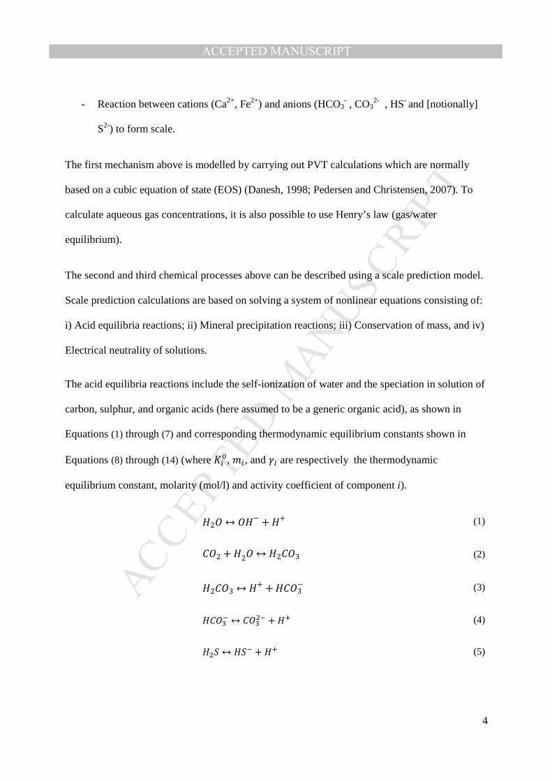
The acid equilibria reactions include the self-ionization of water and the speciation in solution of

carbon, sulphur, and organic acids (here assumed to be a generic organic acid), as shown in

Equations (1) through (7) and corresponding thermodynamic equilibrium constants shown in

Equations (8) through (14) (where ���, ��, and �� are respectively the thermodynamic

equilibrium constant, molarity (mol/l) and activity coefficient of component i).

�2� ↔ ��− + �+ (1)

��2 + �2� ↔ �2��3 (2)

�2��3 ↔ �+ + ���3− (3)

����� ↔ ����� + �� (4)

��� ↔ ��� + �� (5)

MANUSCRIP

T

ACCEPTED

ACCEPTED MANUSCRIPT

5

The species activities in the equilibrium equations in this work are calculated using the Pitzer

model which is described extensively in the literature (Gubbins, 1997; Pitzer, 1975; Pitzer, 1973;

Pitzer, 1986; Pitzer et al., 1984).

In this paper we are only discussing the formation of CaCO3, FeCO3 and FeS which are pH-

dependent scales described by Equations (15) through (17) (the corresponding solubility products

are shown in Equation (18) through (20)) but additional chemical equilibrium equations can be

included for pH-independent scales such as BaSO4, CaSO4, etc.

��� ↔ ��� + �� (6)

�� ↔ �� + �� (7)

����� = (���� × ���)(���� × ���) (8)

����,�� = �����!����

�����!����

(9)

����,�� = ��� × ����!�

�����!��� × ����!�

�����! (10)

����,�� = ��� × ���!��

����!���� × ���!��

����!� (11)

���",�� = ��"� × ��� ���"

��"� × ���

���" (12)

���",�� = ��� × �"��

��"���� × �"��

��"� (13)

��#� = ��� × �#�

��#��� × �#�

��# (14)

MANUSCRIP

T

ACCEPTED

ACCEPTED MANUSCRIPT

6

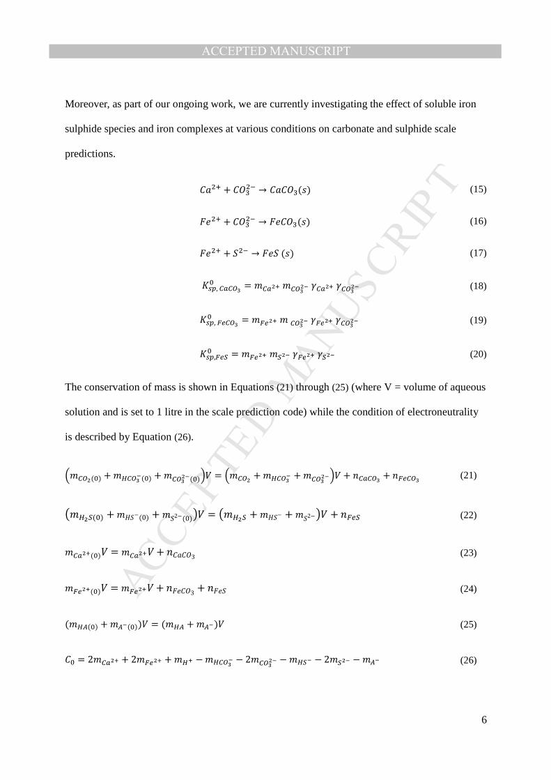
Moreover, as part of our ongoing work, we are currently investigating the effect of soluble iron

sulphide species and iron complexes at various conditions on carbonate and sulphide scale

predictions.

�$�� + ����� → �$���(&) (15)

'(�� + ����� → '(���(&) (16)

'(�� + ��� → '(� (&) (17)

�)*, �+��!� = ��+�� ���!�� ��+�� ���!�� (18)

�)*, ,-��!� = �,-�� � ��!�� �,-�� ���!�� (19)

�)*,,-"� = �,-�� �"�� �,-�� �"�� (20)

The conservation of mass is shown in Equations (21) through (25) (where V = volume of aqueous

solution and is set to 1 litre in the scale prediction code) while the condition of electroneutrality

is described by Equation (26).

.����(�) + ����!�(�) + ���!��(�)/0 = .���� + ����!� + ���!��/0 + 1�+��! + 1,-��! (21)

2���"(�) + ���−(0) + ��2−(0)40 = 2���" + ���− + ��2−40 + 1,-" (22)

��+��(�)0 = ��+��0 + 1�$��3 (23)

�,-��(�)0 = �,-��0 + 1'(��3 + 1'(� (24)

(��#(�) + �#�(�))0 = (��# + �#�)0 (25)

�� = 2��+�� + 2�,-�� + ��� − ����!� − 2���!�� − ��"� − 2�"�� − �#� (26)

MANUSCRIP

T

ACCEPTED

ACCEPTED MANUSCRIPT

7

This system of nonlinear equations can then be solved using the Newton-Raphson algorithm.

The sulphide related Equations (5), (6) and (17) can be re-written into Equations (27) or (29) and

the correlation between solubility products is shown in Equation (29) and (30). Finally, the

temperature dependence of �)*,,-",�� is expressed by Equation (31) (Sun et al., 2008).

'(�� + ��� → '(� ↓ +�� (27)

'(�� + ��� → '(� ↓ +2�� (28)

�)*,,-",�� = �,-�� × ��"�

����,-�� × ��"�

���= �)*,,-"�

���",�� (29)

�)*,,-",�� = �,-�� × ��2�(���)�

�,-�� × ���"(���)� = �)*,,-"�

���",�� × ���",�� (30)

678,9:;,<= = >=?@ABA.DDEFG H−I.<BD

(31)

These sets of equations are implemented in commercial scale prediction models (generally using

an activity model for the electrolytes) which then calculate the Saturation Ratio (SR) (Equation

(32)) for each scale type and determine which scale can form at given conditions and water

chemistry; for example for calcium carbonate, SR is given by.

�J = ��+�� × ���!��

�)*,�+��!� (32)

For SR<1, no scale forms, at SR = 1 the system is at equilibrium and if SR >1, the scale will

form.

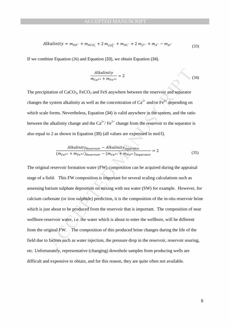
The total alkalinity of this system is defined by Equation (33).

MANUSCRIP

T

ACCEPTED

ACCEPTED MANUSCRIPT

8

�KL$KM1MNO = ���− + ����3− + 2���32− + ���− + 2��2− + ��− − ��+

(33)

If we combine Equation (26) and Equation (33), we obtain Equation (34).

�KL$KM1MNO��+�� + �,-��

= 2 (34)

The precipitation of CaCO3, FeCO3 and FeS anywhere between the reservoir and separator

changes the system alkalinity as well as the concentration of Ca2+ and/or Fe2+ depending on

which scale forms. Nevertheless, Equation (34) is valid anywhere in the system, and the ratio

between the alkalinity change and the Ca2+/ Fe2+ change from the reservoir to the separator is

also equal to 2 as shown in Equation (35) (all values are expressed in mol/l).

�KL$KM1MNOP-)-QRS�Q − �KL$KM1MNO)-*+Q+TSQ(��+�� + �,-��)P-)-QRS�Q − (��+�� + �,-��)"-*+Q+TSQ

= 2 (35)

The original reservoir formation water (FW) composition can be acquired during the appraisal

stage of a field. This FW composition is important for several scaling calculations such as

assessing barium sulphate deposition on mixing with sea water (SW) for example. However, for

calcium carbonate (or iron sulphide) prediction, it is the composition of the in-situ reservoir brine

which is just about to be produced from the reservoir that is important. The composition of near

wellbore-reservoir water, i.e. the water which is about to enter the wellbore, will be different

from the original FW. The composition of this produced brine changes during the life of the

field due to factors such as water injection, the pressure drop in the reservoir, reservoir souring,

etc. Unfortunately, representative (changing) downhole samples from producing wells are

difficult and expensive to obtain, and for this reason, they are quite often not available.

MANUSCRIP

T

ACCEPTED

ACCEPTED MANUSCRIPT

9

On the other hand, real-time surface data (from the wellhead and separator) is usually easier and

cheaper to obtain, and much more of this type of data exists in the oil industry. Of course, this

surface produced brine may already have undergone some scaling reactions (due to loss of CO2

for example), and its ion composition will be different from the same water sample just as it left

the reservoir. Thus, we have to use the produced brine composition to “reconstruct” the

downhole version of this same aqueous fluid element. Equation (35) is one of the constraints

which allows us to calculate near wellbore-reservoir water chemistry from commonly available

surface produced water compositions.

NOTE: if the measured surface values are unreliable, there will be uncertainty around the

reconstructed near wellbore-reservoir water chemistry. However, if the measured values are

unreliable, then any calculation run using these values may give inaccurate results. A good way

to overcome this problem is to run a sensitivity study on the “inaccurate” data and determine if

these values do or do not play an important role in the final scale prediction results.

THEORETICAL CALCULATIONS

The design of a rigorous step-by-step procedure for carbonate and sulphide scale predictions can

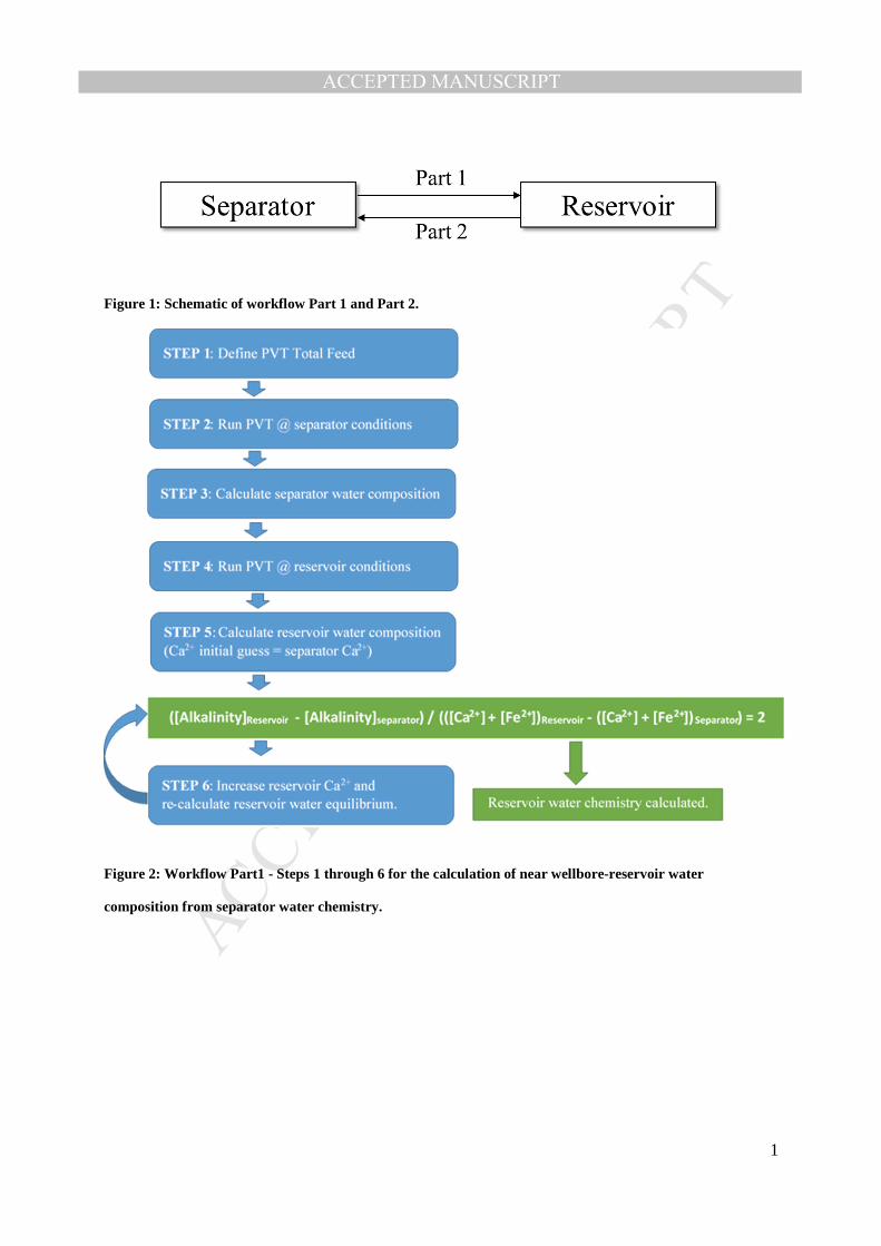
be divided into two main parts (Figure 1):

Part 1. From separator to reservoir: reconstruct near wellbore-reservoir water

chemistry from commonly available surface data.

Part 2. From reservoir to separator: calculate a scale prediction profile from the

reservoir to the separator using the reconstructed near wellbore-reservoir water

chemistry.

MANUSCRIP

T

ACCEPTED

ACCEPTED MANUSCRIPT

10

Due to the uncertainty associated with water soluble iron measurement in sour systems (NACE,

2012) we run the workflow assuming that Fe2+=0. We then apply the concept of Maximum

Dissolved Iron (MDI) which is described in a recent paper (Verri and Sorbie, 2017) and

investigate iron sulphide formation using the water chemistry calculated from this workflow. If

sulphides are not present, Fe2+ can be treated just like an additional cation, and we can follow the

same procedure used below for Ca2+.

PART 1 – FROM SEPARATOR TO RESERVOIR

The recombination process to obtain near wellbore-reservoir water composition from surface

water chemistry can be divided into six steps and is shown in Figure 2. This is based on the

availability of common field data such as separator temperature (T) and pressure (p), reservoir T

and p; well flow rates, well gas CO2 and H2S concentration measured at separator conditions,

produced water chemistry from separator sample and original hydrocarbon PVT.

STEP 1: Obtain PVT total feed.

The PVT total feed is the composition of the combined gas, oil and water phases present in the

system. The PVT total feed may change from reservoir to separator if paraffin and asphaltenes

precipitate/dissolve or if reactions involving CO2 and H2S occur in the water phase.

The total feed must include all system components, and it is particularly important to add the

correct amount of total water, CO2 and H2S present in the system. These values change over time

and must be adjusted if conditions change (i.e. water injection, reservoir souring).

The ways to incorporate water into the hydrocarbon composition (available from original PVT

experimental data) and adjust CO2 and H2S concentration are different for different types of

MANUSCRIP

T

ACCEPTED

ACCEPTED MANUSCRIPT

11

hydrocarbons. These steps may include the tuning of the equations of state (EOS) for oil and gas

phase, or adjustment of the solubility parameters for CO2 and H2S providing experimental data is

available. We addressed this problem in previous publications for gas/condensate well (Verri et

al., 2017a) and for oil wells (Verri et al., 2017b) but other types of fluid may require different

specific calculation steps.

In all scenarios, whether we are using an integrated software package or not, some important

checks may be carried out to ensure that the total feed is calculated correctly. These include but

are not limited to:

- Ensure that the total feed flashed at standard conditions gives the correct GOR. For high

water cut wells, the GWR also plays an important role and the total feed flashed at

standard conditions must produce a gas volume equal to GOR+GWR.

- Ensure that the calculated total feed correctly predicts the oil bubble point.

- If the separator is close to equilibrium conditions (sufficient retention time), the total feed

flashed at separator conditions should give the correct gas/oil/water ratio as well as the

field measured CO2 and H2S gas phase concentration (if these are reliable).

STEP 2: Run PVT calculations at separator conditions.

Using the calculated total PVT feed, run the PVT calculations at separator T and p.

This gives the gas, oil and water molecular CO2 and H2S concentrations at separator conditions

as well as the three-phase relative volume and mole distributions of all relevant components.

MANUSCRIP

T

ACCEPTED

ACCEPTED MANUSCRIPT

12

The gas phase CO2 and H2S concentration and the relative flow rates should match the measured

values.

Knowing the measured flow rates, the three-phase relative flow rates and each phase’s molar

volume, we can calculate the total number of moles of gas + water + oil in the system. We then

keep this value constant from near wellbore-reservoir to separator because the total number of

moles in the system does not change. This total number of moles does not account for other

aqueous species such as HCO3-, CO3

2-, HS- and S2- which can influence changes in molecular

CO2 and H2S moles. Nevertheless, for the field scenarios investigated so far (Verri et al., 2017a;

Verri et al., 2017b) the change in total molecular CO2 and H2S caused by water phase reaction is

negligible when compared to the total number of moles.

STEP 3: Calculate separator water pH, HCO3-, CO3

2-, HS- and S2-

Some PVT software packages only consider the partitioning of molecular CO2 and H2S between

gas, oil and water but do not calculate CO2 and H2S speciation (to HCO3-, CO3

2-, HS- and S2-) or

pH. Hence, we need to use an aqueous scale prediction software code which models the water

phase to calculate these values.

All scale prediction software packages have an “initial” set of input values which are used to

calculate the “final” equilibrium conditions. In this step, we adjust the initial conditions (CO2,

H2S and alkalinity) and fix the final aqueous molecular CO2 and H2S concentration to the values

calculated from the PVT and the final alkalinity and Ca2+ to the measured field values to

calculate the water pH, carbonate and sulphide distribution (HCO3-, CO3

2-, HS- and S2-). These

calculated values fully define the separator water composition.

MANUSCRIP

T

ACCEPTED

ACCEPTED MANUSCRIPT

13

STEP 4: Run PVT at reservoir conditions.

If we assume that asphaltenes and paraffin do not precipitate in the well and that the effect of

chemical reactions involving CO2 and H2S (in this case scale precipitation and

carbonate/sulphide re-speciation at different T and p) is negligible on the total three-phase

molecular CO2 and H2S values, we can use the same PVT total feed at separator and reservoir. If

these differences are not negligible, the reservoir PVT total feed must be adjusted to include

precipitated hydrocarbons and generated/consumed CO2 and H2S.

This calculation gives the gas, oil and water molecular CO2 and H2S concentrations at reservoir

conditions as well as the two/three phase relative volume and mole distributions of all relevant

components.

STEP 5: Calculate reservoir water equilibrium chemistry.

If scale precipitates between the reservoir and separator, the reservoir Ca2+ concentration will be

different from separator Ca2+.

Initially, we guess the reservoir Ca2+ and start by using the same separator Ca2+ concentrations.

We then adjust the initial conditions and fix the final aqueous molecular CO2 and H2S (from

PVT), final Ca2+ (our initial guess value) and the carbonate equilibrium condition CaCO3 SR=1,

to calculate the water pH, carbonate and sulphide distribution (HCO3-, CO3

2-, HS- and S2-).

Finally, we calculate the reservoir alkalinity (Equation (33)) and the result of Equation (35). If

the final value is not 2, carbonate scale has precipitated between the reservoir and separator, and

we need to progress to Step 6.

MANUSCRIP

T

ACCEPTED

ACCEPTED MANUSCRIPT

14

NOTE: Equation (35) uses concentrations in mol/l. If the scale prediction software input is in

ppm (mg/kg), we need to consider the water density changes in our calculations. Hence, the final

Ca2+ (ppm) may be lower in the reservoir than in the separator with scale precipitating along the

wellbore simply because of the density change. Nevertheless, the Ca2+ (mol/l) will be higher.

STEP 6: Increase reservoir Ca2+ and recalculate reservoir water equilibrium chemistry.

In this stage, we increase the reservoir Ca2+ concentration.

We then adjust the initial conditions and fix the final aqueous molecular CO2 and H2S (from

PVT), final Ca2+ (our new guessed value) and the carbonate equilibrium condition CaCO3 SR=1,

to re-calculate the water pH, carbonate and sulphide distribution (HCO3-, CO3

2-, HS- and S2-).

Finally, we calculate the result of Equation (35).

We adjust the reservoir Ca2+ until the results of Equation (35) is exactly 2.

This final near wellbore-reservoir water composition represents the correct and unique chemistry

which produces the measured separator water composition. It also represents our initial water

composition for wellbore scale predictions and will ultimately give the same separator water

chemistry that we started with if we follow the steps of Part 2 of the workflow to now go from

the reservoir to the separator.

PART 2 – FROM RESERVOIR TO SEPARATOR

After obtaining the correct near wellbore-reservoir water composition, we need to define a

rigorous procedure to calculate scale predictions and three phase composition trends from the

reservoir up to the wellbore (accounting for any devices present in the wellbore such as ESPs

[electrical submersible pumps], etc.) to the separator. This is shown in Figure 3.

MANUSCRIP

T

ACCEPTED

ACCEPTED MANUSCRIPT

15

STEP 7: Calculate reservoir total carbonates and sulphides.

In Part 1 of the workflow, we obtained the near wellbore-reservoir water chemistry (CO2 (aq), H2S

(aq), HCO3-, CO3

2-, HS- and S2-), the oil and gas CO2 and H2S (only one hydrocarbon phase may

be present) and the two/three phase relative volumes.

Using this information we can calculate the total system carbonates and sulphides. If we include

any precipitated carbonate and sulphide scale along the well in our calculations, the total

carbonates and sulphides do not change from reservoir to separator. This is important for our

following calculations.

STEP 8: Run PVT at selected T and p interval.

In this calculation, we use the same PVT total feed used at reservoir and separator for the reasons

explained in STEP 4.

This calculation gives the gas/oil/water CO2 and H2S partition coefficients as well as the

two/three phase relative volume and mole distributions of all relevant components at each

selected point in the wellbore.

STEP 9: Run scale predictions at selected T and p interval.

Using the reservoir water chemistry (or the “previous T and p step” water chemistry) as initial

conditions in the scale prediction software, we calculate the final water chemistry and scaling

potential at the new T and p interval selected.

The final resulting water chemistry (CO2 (aq), H2S (aq), HCO3-, CO3

2-, HS- and S2-), and the

oil/water (KOW) and gas/water (KGW) partition coefficients are used to calculate the total system

MANUSCRIP

T

ACCEPTED

ACCEPTED MANUSCRIPT

16

carbonates and sulphides. This calculation must include any precipitated carbonate and sulphide

scale along the well. The number of moles of each phase (gas, oil, water) is calculated fixing the

total number of moles from Step 2 and using the new phase mole % from the PVT calculation at

given T and p.

The calculated total carbonates and sulphides will be different from the original reservoir value

because this simple step looks at the water phase only and does not account for CO2 and H2S

repartitioning in the other phases. This issue is addressed in Step 10.

STEP 10: Adjust initial molecular CO2 and H2S and recalculate final water chemistry.

Like in Step 9, we use the reservoir water chemistry (or the “previous T and p step” water

chemistry) as initial conditions in the scale prediction software but this time we adjust the initial

molecular CO2 and H2S concentration until the final calculated water chemistry gives the correct

total carbonates and sulphides which we obtained at reservoir conditions and which must remain

constant in the wellbore and at the separator. It is important to include any precipitated scale in

the calculation of total system carbonates and sulphides.

By adjusting the initial aqueous molecular CO2 and H2S, we are reproducing the re-partitioning

of molecular CO2 and H2S to other phases (gas and oil), hence looking at the overall mechanisms

which affect a three phase system.

The final water chemistry that provides the correct total carbonates and sulphides represents the

equilibrated water chemistry at the selected T and p interval. This can be used as the initial

condition for the next T and p interval (but reservoir water can also be used). In addition to the

MANUSCRIP

T

ACCEPTED

ACCEPTED MANUSCRIPT

17

water chemistry, we also obtain the saturation ratio, and mass of scale precipitated at the selected

point.

RESULTS – EXAMPLE WELL

For our applied example we used the following data:

- Separator T=65°C p=10 bar

- Reservoir T=90°C p=300 bar

- Separator oil = 3001 BOPD

- Separator water = 193 BWPD

- Separator gas phase CO2 = 2.1%

- Separator gas phase H2S = 2.7%

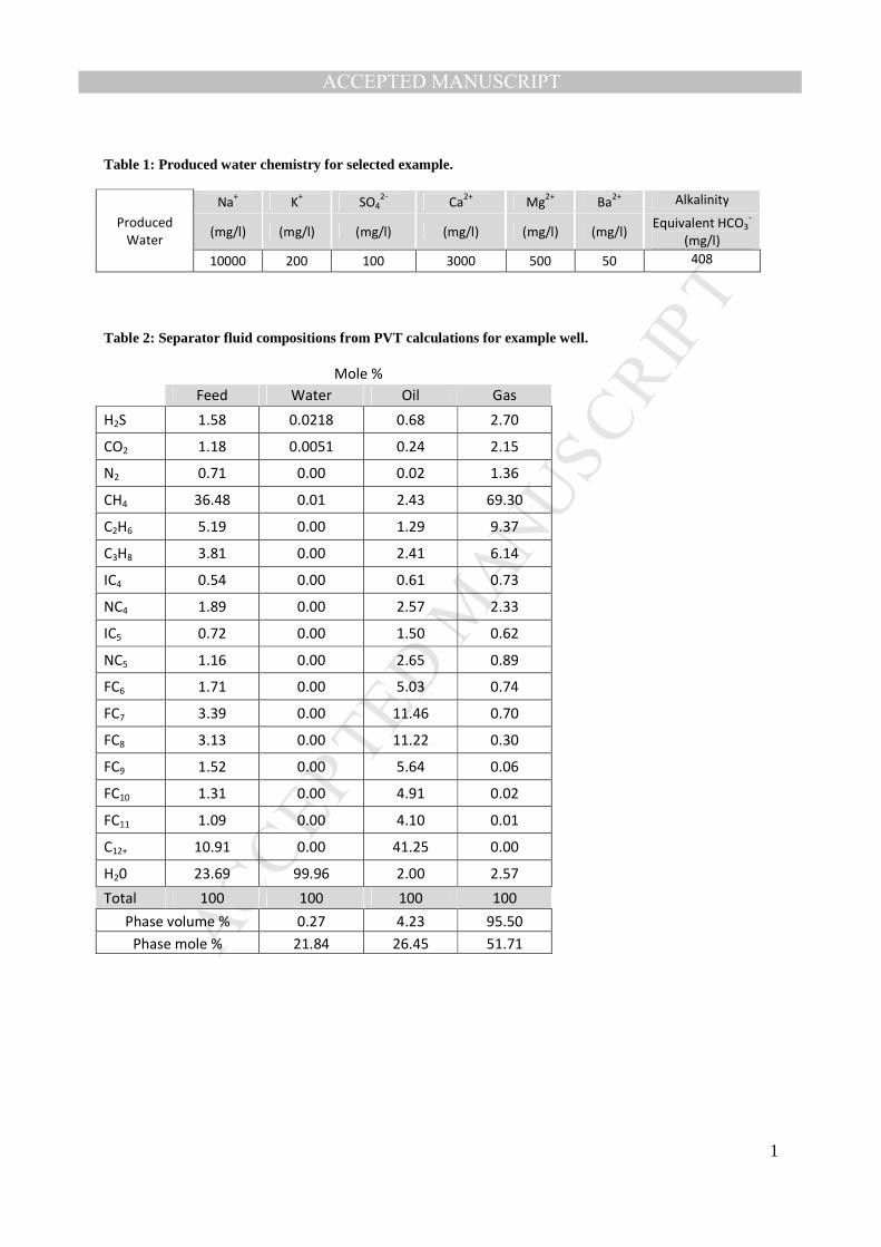
- Produced water chemistry is shown in Table 1.

- C12+ MW = 265

- C12+ SG = 0.88

- Peng-Robinson 1978 EOS

- Other parameters as fixed by Winprop (CMG, 2017)

- Scale software = Heriot-Watt scale prediction software (Silva et al., 2016)

Initially, we do not include Fe2+ in our calculations, but we will account for it at the end of our

calculations using the maximum dissolved iron (MDI) concept (Verri and Sorbie, 2017).

Although other scales which are not pH-dependent may form (i.e. BaSO4) they are not the main

topic of our study and will not be addressed in this discussion. The formation of complexes is

also not included but may play a significant role in some specific scenarios. We will discuss the

effect of these complexes in future publications.

Neither the formation of other types of scale nor the formation of soluble complexes alters the

workflow steps.

MANUSCRIP

T

ACCEPTED

ACCEPTED MANUSCRIPT

18

STEP 1:

As mentioned in the general description of STEP 1, this step depends on the type of fluids that

are being characterised and on the available compositions and experimental PVT data. The

results shown here are for a generic medium API oil field scenario, and the total feed is shown in

Table 2.

STEP 2:

The results of the separator PVT calculations are shown in Table 2. Note that the gas phase CO2

and H2S concentration, as well as the oil/water ratio, must match the separator measured values.

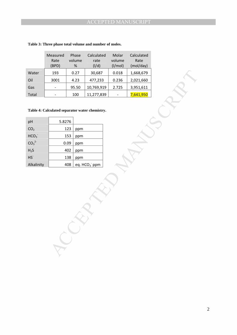
Using the oil and water measured flow rates, the phase volume % and the phase molar volume

obtained from the PVT calculations we can calculate the total number of moles of gas + water +

oil in the system as shown in Table 3. This final value is fixed from reservoir to separator.

STEP 3:

By fixing the final aqueous molecular CO2 and H2S to the concentration given in Table 2 and the

final alkalinity to the measured value, we calculate the separator water chemistry which is shown

in Table 4.

STEP 4

The PVT results at reservoir conditions are shown in Table 5.

MANUSCRIP

T

ACCEPTED

ACCEPTED MANUSCRIPT

19

STEP 5/6

In this step we use the calcium carbonate equilibrium condition (CaCO3 SR=1), fix the final CO2

and H2S given by the PVT results and guess a reservoir Ca2+ concentration (starting with the

same concentration at separator) until Equation (35) is satisfied. Note that the concentrations

used in Equation (35) are expressed in mol/l. The results are shown in Table 6 and the calculated

reservoir water chemistry in Table 7.

STEP 7

In this step, we use the total number of moles (Table 3) and the phase mole % (Table 5) to

calculate the total number of moles of each phase. We then use the reservoir water composition

(Table 7) and the oil and gas CO2 and H2S concentration from PVT to calculate the total number

of moles of carbonates and sulphides shown in Table 8. This number does not change from the

near wellbore-reservoir to the separator as long as we account for any precipitated carbonate and

sulphide scales.

STEP 8

In this step, we run PVT calculations at the selected temperature and pressure conditions.

The T and p steps selected for this example, the resulting oil/water and gas/water partition

coefficients for CO2 and H2S (KOW and KGW expressed in mol fraction/mol fraction) and the

water/oil/gas mole fraction are shown in Table 9.

STEP 9/10

Following the procedure described earlier, we obtain the results shown in Table 10.

MANUSCRIP

T

ACCEPTED

ACCEPTED MANUSCRIPT

20

The calcium carbonate scale prediction profile is also shown in Figure 4.

The separator water composition shown in Table 10 is the recalculated water composition

obtained from the originally calculated reservoir water chemistry. Table 11 shows the relative

error between the initially calculated separator water chemistry (from measured data) and the

recalculated values.

This difference is because CaCO3 precipitation impacts the CO2/HCO3-/CO3

2- equilibrium

(Equation (2), (3), (4) and (15)) and changes the three phase total moles of molecular CO2 hence

changing the PVT total feed. In other words, the PVT total feed slightly changes between

reservoir and separator conditions changing the water phase CO2 and H2S concentrations which

are used in STEP 3 and STEP 5.

Nevertheless, in this scenario and all other scenarios so far investigated the relative error is <10%

and the assumption of constant PVT Total Feed from the reservoir to separator can be used.

IRON ADDITION

Workflow steps 1-10 allow us to obtain a full water chemistry profile as well as calcium

carbonate scale predictions from near wellbore-reservoir to separator.

This data can now be used to calculate sulphide scale prediction using the Maximum Dissolved

Iron (MDI) concept introduced and described in a recent publication (Verri and Sorbie, 2017).

The Maximum Dissolved Iron (MDI) is the maximum concentration of Fe2+ which can

potentially be present in the aqueous phase at given T, p and water chemistry. If the available

MANUSCRIP

T

ACCEPTED

ACCEPTED MANUSCRIPT

21

Fe2+ concentration exceeds MDI, the iron scale is predicted to form (this scale may be FeS or

FeCO3 depending on the system conditions).

In practical terms, we take the calculated water chemistry (Table 10) and add variable

concentrations of Fe2+ until scale precipitates. This concentration represents the MDI.

For the given example MDI<0.1 mg/l at all selected points in the system. This means that if iron

is present in the water (from reservoir fluids, corrosion or other sources), it will be in solid form.

CONCLUSIONS

This paper presents a modelling approach or “workflow” to close the gap between surface and

subsurface fluid modelling by providing chemists/engineers with a clear step-by-step procedure

to produce scale prediction profiles from reservoir to first separation stage using commonly

available field data. Several companies within the oil industry have internal procedures which

they apply to achieve similar goals. However, these procedures are not published and, indeed,

part of the intention of this paper is to have a public discussion of how the industry should be

carrying out these calculations more accurately.

The main discussion focuses on the handling of the CO2/carbonate system, with the concept of

maximum dissolved iron (MDI) being used to address iron sulphide scale predictions.

The choice of software, the equation of state, parameters, etc. is independent of the procedure

and is at the user’s discretion allowing this workflow to be applied to any field scenario

providing that the PVT model is tuned for the given system.

MANUSCRIP

T

ACCEPTED

ACCEPTED MANUSCRIPT

22

At this stage, all calculations assume equilibrium conditions. As part of our future work, we will

investigate the effect of kinetics on the scale prediction results. Also, we are developing an

integrated suite of software to carry out the types of calculation described in this work

automatically. That is, the mineral scaling profile will be calculated at many points from the

reservoir up through the well tubing (and devices in the wells, e.g. ESPs) to the separator, thus

giving a near continuous calculation of the scale type and amount.

AUTHOR INFORMATION

Main Author and Corresponding Author

Giulia Verri, PhD Student

Heriot-Watt University, Edinburgh Campus, Edinburgh EH14 4AS

Email: gv6@hw.ac.uk

Phone: +44(0)1314514581

Co-Authors

Kenneth S. Sorbie, k.sorbie@hw.ac.uk

Duarte Silva, ds288@hw.ac.uk

ACKNOWLEDGMENT

The authors would like to thank the Flow Assurance and Scale Team (FAST) JIP sponsors:

Halliburton Multi-Chem, Nalco Champion, Petronas, Repsol Sinopec, Schlumberger MI Swaco,

Shell, Statoil, Total and Wintershall. The authors would also like to thank CMG for the use of

Winprop PVT Software.

MANUSCRIP

T

ACCEPTED

ACCEPTED MANUSCRIPT

23

ABBREVIATIONS

EOS = Equation of State, KGW = gas/water partition coefficient, KOW = oil/water partition

coefficient, MDI = Maximum Dissolved Iron, PVT = Pressure/Volume/Temperature, SR=

Saturation Ratio.

REFERENCES

Amend, J.P., Edwards, K.J. and Lyons, T.W., 2004. Sulfur Biogeochemistry - Past and Present. The Geological Society of America, Boudler, CO.

Calsep, 2015. PVTsim NOVA. CMG, 2017. Winprop. Danesh, A., 1998. PVT and Phase Behaviour of Petroleum Reservoir Fluids. Elsevier. Expro, 2015. MultiScale. Gubbins, K.E., 1997. Thermodynamics. By K. S. Pitzer, 3rd ed. AIChE Journal, 43(1): 285. NACE, 2012. Monitoring Corrosion in Oil and Gas Production with Iron Counts. NACE. Nasr-El-Din, H.A. and Al-Humaidan, A.Y., 2001. Iron Sulfide Scale: Formation Removal and

Prevention, International Symposium on Oilfield Scale, Aberdeen, United Kingdom. Olajire, A.A., 2015. A review of oilfield scale management technology for oil and gas

production. Journal of Petroleum Science and Engineering, 135: 723-737. OLI, 2016. ScaleChem. Pedersen, K.S. and Christensen, p.L., 2007. Phase Behaviour of petroleoum reservoir fluids. Pitzer, K., 1975. Thermodynamics of electrolytes. V. effects of higher-order electrostatic terms. J

Solution Chem, 4(3): 249-265. Pitzer, K.S., 1973. Thermodynamics of electrolytes. I. Theoretical basis and general equations.

The Journal of Physical Chemistry, 77(2): 268-277. Pitzer, K.S., 1986. Theoretical considerations of solubility with emphasis on mixed aqueous

electrolytes. Pure and Applied Chemistry, 58(12): 1599-1610. Pitzer, K.S., Peiper, J.C. and Busey, R.H., 1984. Thermodynamic Properties of Aqueous Sodium

Chloride Solutions. Journal of Physical and Chemical Reference Data, 13(1): 1-102. Silva, D., Sorbie, K.S. and Mackay, E.J., 2016. Modelling CaCO3 Scale in CO2 Water

Alternating Gas CO2-WAG Processes, SPE International Oilfield Scale Conference and Exhibition. Society of Petroleum Engineers, Aberdeen, Scotland.

Sun, W., Nešić, S., Young, D. and Woollam, R.C., 2008. Equilibrium Expressions Related to the Solubility of the Sour Corrosion Product Mackinawite. Industrial and Engineering Chemistry Research, 47(5): 1738-1742.

Verri, G. and Sorbie, K.S., 2017. Iron Sources in Sour Wells: Reservoir Fluids or Corrosion?, NACE Corrosion. NACE, New Orleans.

Verri, G. et al., 2017a. Iron Sulfide Scale Management in High-H2S and -CO2 Carbonate Reservoirs. SPE Production & Operations.

Verri, G. et al., 2017b. A New Approach to Combined Sulphide and Carbonate Scale Predictions Applied to Different Field Scenarios Oilfield Chemistry Conference, Montgomery, TX.

MANUSCRIP

T

ACCEPTED

ACCEPTED MANUSCRIPT

1

Table 1: Produced water chemistry for selected example.

Produced

Water

Na+ K

+ SO4

2- Ca

2+ Mg

2+ Ba

2+ Alkalinity

(mg/l) (mg/l) (mg/l) (mg/l) (mg/l) (mg/l) Equivalent HCO3

-

(mg/l)

10000 200 100 3000 500 50 408

Table 2: Separator fluid compositions from PVT calculations for example well.

Mole %

Feed Water Oil Gas

H2S 1.58 0.0218 0.68 2.70

CO2 1.18 0.0051 0.24 2.15

N2 0.71 0.00 0.02 1.36

CH4 36.48 0.01 2.43 69.30

C2H6 5.19 0.00 1.29 9.37

C3H8 3.81 0.00 2.41 6.14

IC4 0.54 0.00 0.61 0.73

NC4 1.89 0.00 2.57 2.33

IC5 0.72 0.00 1.50 0.62

NC5 1.16 0.00 2.65 0.89

FC6 1.71 0.00 5.03 0.74

FC7 3.39 0.00 11.46 0.70

FC8 3.13 0.00 11.22 0.30

FC9 1.52 0.00 5.64 0.06

FC10 1.31 0.00 4.91 0.02

FC11 1.09 0.00 4.10 0.01

C12+ 10.91 0.00 41.25 0.00

H20 23.69 99.96 2.00 2.57

Total 100 100 100 100

Phase volume % 0.27 4.23 95.50

Phase mole % 21.84 26.45 51.71

MANUSCRIP

T

ACCEPTED

ACCEPTED MANUSCRIPT

2

Table 3: Three phase total volume and number of moles.

Measured

Rate

(BPD)

Phase

volume

%

Calculated

rate

(l/d)

Molar

volume

(l/mol)

Calculated

Rate

(mol/day)

Water 193 0.27 30,687 0.018 1,668,679

Oil 3001 4.23 477,233 0.236 2,021,660

Gas - 95.50 10,769,919 2.725 3,951,611

Total - 100 11,277,839 - 7,641,950

Table 4: Calculated separator water chemistry.

pH 5.8276

CO2 123 ppm

HCO3- 153 ppm

CO32-

0.09 ppm

H2S 402 ppm

HS- 138 ppm

Alkalinity 408 eq. HCO3- ppm

MANUSCRIP

T

ACCEPTED

ACCEPTED MANUSCRIPT

3

Table 5: Reservoir PVT results for example well.

Mole %

Feed Water Oil

H2S 1.58 0.1652 1.99

CO2 1.18 0.0367 1.51

N2 0.71 0.00 0.92

CH4 36.48 0.18 46.98

C2H6 5.19 0.01 6.69

C3H8 3.81 0.00 4.92

IC4 0.54 0.00 0.69

NC4 1.89 0.00 2.43

IC5 0.72 0.00 0.93

NC5 1.16 0.00 1.50

FC6 1.71 0.00 2.21

FC7 3.39 0.00 4.38

FC8 3.13 0.00 4.03

FC9 1.52 0.00 1.96

FC10 1.31 0.00 1.69

FC11 1.09 0.00 1.40

C12+ 10.91 0.00 14.07

H20 23.69 99.61 1.72

Total 100 100 100

Phase volume % 4.23 95.77

Phase mole % 22.44 77.56

Table 6: Results of Equation (23) for different concentrations of reservoir Ca2+.

Reservoir Ca2+

(ppm)

Reservoir Ca2+

(mol/l)

Reservoir Alkalinity

(eq. HCO3- ppm)

Reservoir Alkalinity

(mol/l)

Result of

Equation 23

3000 0.07472 1438 0.02357 -43.56

3357 0.08362 1374 0.02253 1.86

3334 0.08304 1381 0.02264 2.01

MANUSCRIP

T

ACCEPTED

ACCEPTED MANUSCRIPT

4

Table 7: Calculated reservoir water chemistry.

pH 5.3056

CO2 875 ppm

HCO3- 393 ppm

CO32-

0.15 ppm

H2S 3047 ppm

HS- 535 ppm

Ca2+

3334 ppm

Table 8: Total number of moles of water, oil, carbonates and sulphides at reservoir conditions.

Mole

Near wellbore reservoir Water 1,715,106

Near wellbore-reservoir Oil 5,926,844

Carbonates (3 phase) 90,102

Sulphides (3 phase) 121,182

Table 9: Selected T and p steps and corresponding PVT results.

T(°C) p(bar)

KOW

(CO2)

KGW

(CO2)

KOW

(H2S)

KGW

(H2S)

Water

(Mole %)

Oil

(Mole %)

Gas

(Mole %)

Reservoir 90 300 41 - 12 - 22.4 77.6 0.0

Step 1 87 270 42 41 13 10 22.5 75.3 2.2

Step 2 83 210 44 45 17 11 22.6 62.5 14.9

Step 3 78 150 45 52 20 14 22.7 52.2 25.1

Step 4 73 90 46 68 25 19 22.8 42.6 34.6

Separator 65 10 48 419 31 124 21.8 26.5 51.7

Table 10: Calculated water chemistry and scale prediction result from the near wellbore-reservoir to the

separator.

pH Ca2+

CO2 (aq) HCO3- CO3

2-H2S (aq) HS

- CaCO3 CaCO3

MANUSCRIP

T

ACCEPTED

ACCEPTED MANUSCRIPT

5

(ppm) (ppm) (ppm) (ppm) (ppm) (ppm) (SR) (mg/l)

Reservoir 5.31 3334 875 393 0.15 3047 535 1.0 0

Step 1 5.32 3298 856 397 0.14 2761 478 1.2 82

Step 2 5.35 3246 819 387 0.13 2372 398 1.4 128

Step 3 5.38 3201 762 378 0.12 2033 335 1.3 103

Step 4 5.44 3160 643 351 0.11 1689 286 1.3 95

Separator 5.85 3007 122 160 0.10 403 145 1.5 369

Table 11: Relative error between originally calculated separator water chemistry and new recalculated

composition from reservoir water.

Expected Recalculated Relative Error

pH 5.83 5.85 0.35%

CO2 (ppm) 123 122 0.13%

HCO3- (ppm) 153 160 4.82%

H2S (ppm) 402 403 0.32%

HS- (ppm) 138 145 5.14%

Ca2+

(ppm) 3000 3007 0.22%

MANUSCRIP

T

ACCEPTED

ACCEPTED MANUSCRIPT

1

Figure 1: Schematic of workflow Part 1 and Part 2.

Figure 2: Workflow Part1 - Steps 1 through 6 for the calculation of near wellbore-reservoir water

composition from separator water chemistry.

MANUSCRIP

T

ACCEPTED

ACCEPTED MANUSCRIPT

2

Figure 3: Workflow Part 2 - Steps 7 through 10 for the calculation of a scale prediction profile from the

reservoir to the separator.

Figure 4: CaCO3 SR and mass scale prediction trend from reservoir to separator.

0

50

100

150

200

250

300

350

400

0.0

0.2

0.4

0.6

0.8

1.0

1.2

1.4

1.6

1.8

Reservoir Step 1 Step 2 Step 3 Step 4 Separator

Ca

CO

3(m

g/l

)

Ca

CO

3(S

R)

Wellbore steps

CaCO3 SR CaCO3 (mg/l)

MANUSCRIP

T

ACCEPTED

ACCEPTED MANUSCRIPT

• A rigorous procedure for the prediction of carbonate and sulphide scaling profiles from

reservoir to separator is described.

• A new equation is derived to correlate surface water chemistry (post-scaling) to reservoir

water chemistry (pre-scaling) closing the gap between surface and subsurface calculations.

• This procedure can be applied to any field scenario providing a compositional phase

behaviour model is available.