a riemann-hilbert approach to the kundu-eckhaus equation
TRANSCRIPT
A Riemann-Hilbert Approach to the Kundu-Eckhaus
Equation on the half-Line
Bei-bei Hua,b , Tie-cheng Xiaa,∗, Ning Zhanga,c
aDepartment of Mathematics, Shanghai University, Shanghai 200444, China
bSchool of Mathematics and Finance, Chuzhou University, Anhui 239000, China
cDepartment of Basical Courses, Shandong University of Science and Technology, Taian 271019, China
Abstract: In this paper, we consider the initial-boundary value problem of the Kundu-
Eckhaus equation on the half-line by using of the Fokas unified transform method. Assuming
that the solution u(x, t) exists, we show that it can be expressed in terms of the unique so-
lution of a matrix Riemann-Hilbert problem formulated in the plane of the complex spectral
parameter λ. Moreover, we also get that some spectral functions are not independent and
satisfy the so-called global relation.
Keywords: Riemann-Hilbert problem; Kundu-Eckhaus equation; Jump matrix; Fokas uni-
fied transform method
PACS numbers 02.30.Ik, 02.30.Jr, 03.65.Nk
MSC(2010) 35G31, 35Q15, 35Q51
1 Introduction
It is well known that the inverse scattering transformation (IST) is an important method for
analysis initial value problems of integrable nonlinear equations in mathematical physics.
However, in many experimental environment and field situations, the wave motion is initiated
by what corresponds to the imposition of boundary value conditions rather than initial value
conditions. This naturally leads to consider the formulation of initial-boundary value (IBV)
problems instead of a pure initial value problems.
In 1997, Fokas announced a new unified approach based on the Riemann-Hilbert fac-
torization problem to analysis the IBV problems for linear and nonlinear integrable PDEs
[1, 2, 3], we call that Fokas unified transform method. This method provides an important
∗Corresponding author. E-mails: [email protected]; [email protected]; [email protected]
1
arX
iv:1
711.
0251
6v2
[nl
in.S
I] 2
3 N
ov 2
017
generalization of the IST formalism from initial value to IBV problems, and over the last 20
years, this method has been used to analyse boundary value problems for several of the most
important integrable equations possessing 2 × 2 Lax pairs, such as the KdV, the nonlinear
Schrodinger(NLS), the sine-Gordon and the stationary axisymmetric Einstein equations and
so on [4-15]. In 2012, Lenells first extended the Fokas unified transform method to the IBV
problem for the 3× 3 matrix Lax pair [16, 17]. After that, more and more researchers begin
to pay attention to studying IBV problems for integrable evolution equations with higher
order Lax pairs on the half-line or on the interval, the IBV problem for the many integrable
equations with 3×3 or 4×4 Lax pairs are studied, such as, the Degasperis-Procesi equation
[17, 18], the Sasa-Satsuma equation [19], the three wave equation [20], the coupled NLS
equation [21], the vector modified KdV equation [22], the Novikov equation [23], the general
coupled NLS equation[24]. the integrable spin-1 Gross-Pitaevskii equations with a 4×4 Lax
pair [25]. These authors have also done some works about the IBV problem for integrable
equations with 2 × 2 or 3 × 3 Lax pairs on the half-line [13, 26, 27]. Just like the IST
on the line, the Fokas unified transform method yields an expression for the solution of an
IBV problem in terms of the solution of a Riemann-Hilbert problem (RHP). In particular,
the asymptotic behaviour of the solution can be analysed in an effective way by using this
Riemann-Hilbert problem and by employing the nonlinear version of the steepest descent
method introduced by Deift and Zhou [28].
In this paper, we consider Kundu-Eckhaus(KE) equation as follows
iut + uxx + 2|u|2u+ 4β2|u|4u− 4iβ(|u|2)xu = 0, β ∈ R, (1.1)
where u(x, t) is the complex smooth envelop function, t and x are the temporal and spa-
tial variables, respectively, and the last term represents the Raman effect, which accounts
for the self-frequency shift of the waves in optics. The KE equation is an integrable equa-
tion and introduced independently during 1984 by Kundu [29] and later by Calogero and
Eckhaus [30] from different perspective. The KE equation has been studied extensively on
the integrability associated with explicit form of the Lax pair and Painleve property [31],
Hamiltonian structure [32], higher order extension [33], Miura transformation [34], infinitely
many conservation laws [35], soliton given by the bilinear method [36] and other methods
[37-40], rogue waves solutions given by the DT method [41-45].
Recently, Zhu etal. present a RHP formalism for the initial value problem of the KE
equation on the line and using the Deift-Zhou nonlinear steepest descent method to analyzed
the long-time asymptotic for the solutions of the KE equation in [46]. But the IBV problem
of the KE equation on the half-line has not been studied. Therefore, we analyse the IBV
problem of the KE equation on the half-line by using the Fokas unified transform method
in this paper. That it to say, in the quarter (x; t)-plane
Ω = (x, t)|0 < x <∞, 0 < t < T
2
Assume that the solution u(x; t) of the KE equation exists, and the initial-boundary values
data are defined as follows
Initial values: u0(x) = u(x, t = 0), 0 < x <∞;
Boundary values: g0(t) = u(x = 0, t), g1(t) = ux(x = 0, t), 0 < t < T.(1.2)
We will show that u(x, t) can be expressed in terms of the unique solution of a matrix
RHP formulated in the plane of the complex spectral parameter λ. The jump matrix has
explicit (x, t) dependence and is given in terms of the spectral functions a(λ), b(λ) and
A(λ), B(λ), which obtained from the initial data u0(x) = u(x, 0) and the boundary data
g0(t) = u(0, t), g1(t) = ux(0, t), respectively. The problem has the jump across Imλ2 = 0.The spectral functions are not independent, but related by a compatibility condition, the
so-called global relation, which is an algebraic equation coupling a(λ), b(λ) and A(λ), B(λ).
Where a different RHP was formulated and a different representation of the solution of the
KE equation was given, which are more convenient for studying the long-time asymptotic
behavior for the solutions of the KE equation with the decay initial and boundary values lie
in the Schwartz class.
Organization of this paper is as follows. In section 2, some summary results and the
basic RHP of the KE equation are given. In section 3, the spectral functions a(λ), b(λ)
and A(λ), B(λ) are investigated and the RHP is presented. The last section is devoted to
conclusions and discussions.
2 Spectral analysis
We consider the following Lax pair of the KE equation [43]:φx = Mφ,
φt = Nφ = (λ2N2 + λN1 +N0)φ,(2.1)
where
M =
(−iλ+ iβ|u|2 u
−u iλ− iβ|u|2
), N2 =
(−2i 0
0 2i
), N1 =
(0 2u
−2u 0
),
N0 =
(β(−uxu+ uux) + 4iβ2|u|4 + i|u|2 iux + 2β|u|2u
iux − 2β|u|2u β(uxu− uux)− 4iβ2|u|4 − i|u|2
).
(2.2)
In the following section, we set β = 1 and introducing
σ3 =
(1 0
0 −1
), σ1 =
(1 0
0 0
), Q =
(0 u
−u 0
), (2.3)
for the convenient of the analysis, where σ3 denotes the third Pauli’s matrix.
3
2.1 Transformed Lax pair for the KE equation
We can rewrite the Lax pair (2.1) in a matrix formφx + iλσ3φ = U1φ,
φt + 2iλ2σ3φ = U2φ,(2.4)
where U1 = −iQ2σ3 +Q and U2 = 2λQ+ [Qx, Q] + 4iQ4σ3 − iQ2σ3 − iQxσ3 − 2Q3.
Setting
φ = ψe−i(λx+2λ2t)σ3 , 0 < x <∞, 0 < t < T. (2.5)
Then, we have the equivalent Lax pairψx + iλ[σ3, ψ] = U1ψ,
ψt + 2iλ2[σ3, ψ] = U2ψ,(2.6)
which can be written as
d(ei(λx+2λ2t)σ3)ψ(x, t;λ)) = W1(x, t;λ), 0 < x <∞, 0 < t < T, (2.7)
where
W1(x, t;λ) = ei(λx+2λ2t)σ3(U1dx+ U2dt)ψ(x, t;λ), (2.8)
and σ3 denotes the matrix commutator with σ3, σ3A = [σ3, A], then exp(σ3) can be easily
computed: eσ3A = eσ3Ae−σ3 , where A is a 2× 2 matrix.
Next, we consider that a solution of Eq.(10) is of the form
ψ(x, t;λ) = D0 +D1
λ+O(
1
λ2), λ→∞. (2.9)
Substituting Eq.(2.9) into the first equation of (2.6), and comparing the cofficient of λ yields
λ1 : i[σ3, D0] = 0,
λ0 : D0x + i[σ3, D1] = (−iQ2σ3 +Q)D0,
λ−1 : D1x = (−iQ2σ3 +Q)D1.
(2.10)
We know that D0 is a diagonal matrix form O(λ1), and set
D0 =
(D11
0 0
0 D220
).
From O(λ0) we have
D(o)1 =
(0 − i
2uD22
0
− i2uD11
0 0
), D0x = i|u|2σ3D0, (2.11)
4
where D(o)1 being the off-diagonal part of D1. On the other hand, substituting Eq.(2.9) into
the second equation of (2.6), and comparing the cofficient of λ yields
λ2 : 2i[σ3, D0] = 0,
λ1 : 2i[σ3, D1] = 2QD0,
λ0 : D0t = ([Qx, Q] + 4iQ4σ3 − iQ2σ3 − iQxσ3 − 2Q3)D0 + 2QD1,
λ−1 : D1t = ([Qx, Q] + 4iQ4σ3 − iQ2σ3 − iQxσ3 − 2Q3)D1.
(2.12)
After a lengthy calculation, we get
D0t = (−uxu+ uux + 4i|u|4)σ3D0. (2.13)
The Eq.(2.1) have the following conservation law
i(uu)t = (uxu− uux + 4iu2u2)x.
Then Eq.(2.11) and Eq.(2.13) for D0 are consistent and are both satisfied if we define
D0(x, t) = exp(i
∫ (x,t)
(x0,t0)
∆(x, t)σ3), (2.14)
where ∆ is the closed real-valued one-form, and it is given by
∆(x, t) = ∆1dx+ ∆2dt = uudx+ (4u2u2 − i(uux − uxu))dt, (x0, t0) ∈ D,
simultaneity, we let (x0, t0) = (0, 0) for the convenience of calculation.
Noting that the integral in Eq.(2.14) is independent of the path of integration and the
∆ is independent of λ, then we can introduce a new function µ(x, t;λ) as follows
ψ(x, t;λ) = ei∫ (x,t)(0,0)
∆σ3µ(x, t;λ)D0(x, t), 0 < x <∞, 0 < t < T. (2.15)
Then the Lax pair of Eq.(2.7) can be written by
d(ei(λx+2λ2t)σ3µ(x, t;λ)) = W2(x, t;λ), λ ∈ C, (2.16)
where
W2(x, t;λ) = ei(λx+2λ2t)σ3V (x, t;λ)µ(x, t;λ),
V (x, t;λ) = V1(x, t;λ)dx+ V2(x, t;λ)dt = e−i∫ (x,t)(0,0)
∆σ3(U1dx+ U2dt− i∆σ3).(2.17)
By U(x, t;λ) and ∆, we can get
V1(x, t;λ) =
(0 ue−2i
∫ (x,t)(0,0)
∆
−ue2i∫ (x,t)(0,0)
∆ 0
),
5

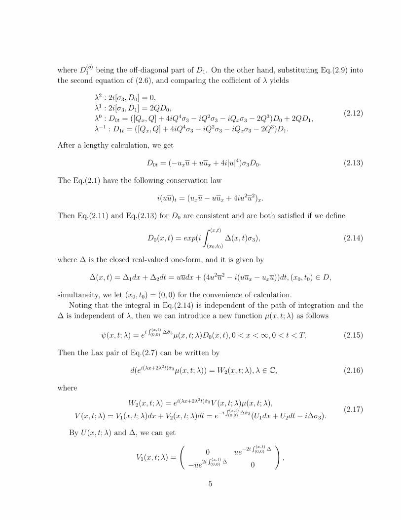
Figure 1: The three contours γ1, γ2, γ3 in the (x, t)-domaint
and
V2(x, t;λ) =
(i|u|2 + 2uux − 2uxu (2λu+ iux + 2u|u|2)e−2i
∫ (x,t)(0,0)
∆
(−2λu+ iux − 2u|u|2)e2i∫ (x,t)(0,0)
∆ −i|u|2 − 2uux + 2uxu
).
Then Eq.(2.16) can be written asµx + iλ[σ3, µ] = V1µ,
µt + 2iλ2[σ3, µ] = V2µ,(2.18)
where 0 < x <∞, 0 < t < T, λ ∈ C.
2.2 Eigenfunctions and Some Relations
Suppose that u(x, t) sufficiently smooth in D = 0 < x < ∞, 0 < t < T, µj(x, t, λ)(j =
1, 2, 3.) are the 2 × 2 matrix valued functions, and we defined the three eigenfunctions
µj(x, t, λ)(j = 1, 2, 3.) of (2.18) by the integral equations
µj(x, t;λ) = I +
∫ (x,t)
(xj ,tj)
e−i(λx+2λ2t)σ3W2(ξ, τ, λ), 0 < x <∞, 0 < t < T, (2.19)
where the integral denotes a smooth curve from (xj, tj) to (x, t), and (x1, t1) = (0, T ), (x2, t2) =
(0, 0), (x3, t3) = (∞, t) (see Figure 1).
Since Eq.(2.19)are independent of the path of integration, we choose the specific contours
depicted in Figure 1 yieldsµ1(x, t;λ) = I +
∫ x0eiλ(ξ−x)σ3(V1µ1)(ξ, t, λ)dξ − e−iλxσ3
∫ Tte2iλ2(τ−t)σ3(V2µ1)(0, τ, λ)dτ,
µ2(x, t;λ) = I +∫ x
0eiλ(ξ−x)σ3(V1µ2)(ξ, t, λ)dξ + e−iλxσ3
∫ t0e2iλ2(τ−t)σ3(V2µ2)(0, τ, λ)dτ,
µ3(x, t;λ) = I −∫∞xeiλ(ξ−x)σ3(V1µ3)(ξ, t, λ)dξ.
(2.20)
The first column of the matrix Eq.(2.19) involves e−2i[λ(ξ−x)+2λ2(τ−t)], and we have the
6
following inequalities on the contours:
γ1 : 0 < ξ < x, t < τ < T,
γ2 : 0 < ξ < x, 0 < τ < t,
γ3 : 0 < x <∞.(2.21)
So, these inequalities imply that the first column of the functions µj(x, t;λ)(j = 1, 2, 3.) are
bounded and analytical for λ ∈ C such that λ belongs to
µ(1)1 (x, t;λ) : Imλ ≥ 0 ∩ Imλ2 ≤ 0,µ
(1)2 (x, t;λ) : Imλ ≥ 0 ∩ Imλ2 ≥ 0,µ
(1)3 (x, t;λ) : Imλ ≤ 0.
(2.22)
In the same way, the second column of the matrix Eq.(2.19) involves the inverse of the above
exponential, which is bounded and analytical in
µ(2)1 (x, t;λ) : Imλ ≤ 0 ∩ Imλ2 ≥ 0,µ
(2)2 (x, t;λ) : Imλ ≤ 0 ∩ Imλ2 ≤ 0,µ
(2)3 (x, t;λ) : Imλ ≥ 0.
(2.23)
Then, we obtain
µ1(x, t;λ) = (µD21 (x, t;λ), µD3
1 (x, t;λ)),
µ2(x, t;λ) = (µD12 (x, t;λ), µD4
2 (x, t;λ)),
µ3(x, t;λ) = (µD3∪D43 (x, t;λ), µD1∪D2
3 (x, t;λ)),
(2.24)
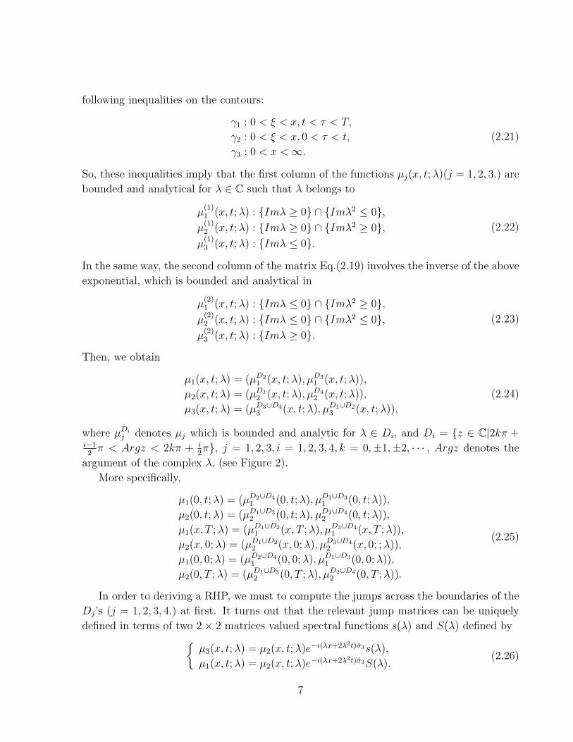
where µDij denotes µj which is bounded and analytic for λ ∈ Di, and Di = z ∈ C|2kπ +i−1
2π < Argz < 2kπ + i
2π, j = 1, 2, 3, i = 1, 2, 3, 4, k = 0,±1,±2, · · · , Argz denotes the
argument of the complex λ, (see Figure 2).
More specifically,
µ1(0, t;λ) = (µD2∪D41 (0, t;λ), µD1∪D3
1 (0, t;λ)),
µ2(0, t;λ) = (µD1∪D32 (0, t;λ), µD2∪D4
2 (0, t;λ)),
µ1(x, T ;λ) = (µD1∪D21 (x, T ;λ), µD3∪D4
1 (x, T ;λ)),
µ2(x, 0;λ) = (µD1∪D22 (x, 0;λ), µD3∪D4
2 (x, 0; ;λ)),
µ1(0, 0;λ) = (µD2∪D41 (0, 0;λ), µD1∪D3
1 (0, 0;λ)),
µ2(0, T ;λ) = (µD1∪D32 (0, T ;λ), µD2∪D4
2 (0, T ;λ)).
(2.25)
In order to deriving a RHP, we must to compute the jumps across the boundaries of the
Dj’s (j = 1, 2, 3, 4.) at first. It turns out that the relevant jump matrices can be uniquely
defined in terms of two 2× 2 matrices valued spectral functions s(λ) and S(λ) defined byµ3(x, t;λ) = µ2(x, t;λ)e−i(λx+2λ2t)σ3s(λ),
µ1(x, t;λ) = µ2(x, t;λ)e−i(λx+2λ2t)σ3S(λ).(2.26)
7
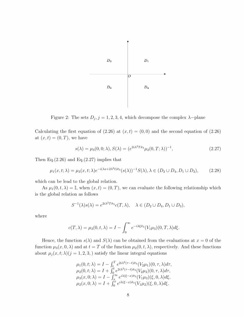
Figure 2: The sets Dj, j = 1, 2, 3, 4, which decompose the complex λ−plane
Calculating the first equation of (2.26) at (x, t) = (0, 0) and the second equation of (2.26)
at (x, t) = (0, T ), we have
s(λ) = µ3(0, 0;λ), S(λ) = (e2iλ2T σ3µ2(0, T ;λ))−1, (2.27)
Then Eq.(2.26) and Eq.(2.27) implies that
µ1(x, t;λ) = µ3(x, t;λ)e−i(λx+2λ2t)σ3(s(λ))−1S(λ), λ ∈ (D2 ∪D4, D1 ∪D3), (2.28)
which can be lead to the global relation.
As µ1(0, t, λ) = I, when (x, t) = (0, T ), we can evaluate the following relationship which
is the global relation as follows
S−1(λ)s(λ) = e2iλ2T σ3c(T, λ), λ ∈ (D2 ∪D4, D1 ∪D3),
where
c(T, λ) = µ3(0, t, λ) = I −∫ ∞
0
e−iλξσ3(V1µ3)(0, T, λ)dξ.
Hence, the function s(λ) and S(λ) can be obtained from the evaluations at x = 0 of the
function µ3(x, 0, λ) and at t = T of the function µ2(0, t, λ), respectively. And these functions
about µj(x, t;λ)(j = 1, 2, 3, ) satisfy the linear integral equations
µ1(0, t;λ) = I −∫ Tte2iλ2(τ−t)σ3(V2µ1)(0, τ, λ)dτ,
µ2(0, t;λ) = I +∫ t
0e2iλ2(τ−t)σ3(V2µ2)(0, τ, λ)dτ,
µ3(x, 0;λ) = I −∫∞xeiλ(ξ−x)σ3(V1µ3)(ξ, 0, λ)dξ,
µ2(x, 0;λ) = I +∫ x
0eiλ(ξ−x)σ3(V1µ2)(ξ, 0, λ)dξ.
8
Let u0(x) = u(x, 0), g0(t) = u(0, t), and g1(t) = ux(0, t) be the initial and boundary values
of u(x, t), respectively. u0(x) = u(x, 0), g0(t) = u(0, t), and g1(t) = ux(0, t) be the initial
and boundary values of u(x, t), respectively. Then, we have
V1(x, 0;λ) =
(0 u0e
−2i∫ x0 |u0|2dξ
−u0e2i
∫ x0 |u0|2dξ 0
),
V2(0, t;λ) =
(i|g0|2 + 2g0g1 − 2g1g0 V
(12)2 (0, t;λ)
V(21)
2 (0, t;λ) −i|g0|2 − 2g0g1 + 2g1g0
),
(2.29)
where
V(12)
2 (0, t;λ) = (2λg0 + ig1 + 2|g0|2g0)e−2i∫ t0 ∆0(0,τ)dτ ,
V(21)
2 (0, t;λ) = (−2λg0 + ig1 − 2|g0|2g0)e2i∫ t0 ∆0(0,τ)dτ ,
with
∆0(0, τ) = 4|g0(τ)|2 − i(g0(τ)g1(τ)− g1(τ)g0(τ)).
The analytic properties of 2 × 2 matrices µj(x, t;λ)(j = 1, 2, 3.) that come from Eq.(2.19)
are collected in the following proposition. We denote by µ(1)j (x, t;λ) and µ
(2)j (x, t;λ) the first
and second columns of µj(x, t;λ), respectively.
Setting
µj(x, t;λ) = (µ(1)j (x, t;λ), µ
(2)j (x, t;λ)) =
(µ11j µ12
j
µ21j µ22
j
), j = 1, 2, 3.
Proposition 2.1 The matrices µj(x, t;λ) = (µ(1)j (x, t;λ), µ
(2)j (x, t;λ))(j = 1, 2, 3.) have the
following properties
• detµ1(x, t;λ) = detµ2(x, t;λ) = detµ3(x, t;λ) = 1;
• µ(1)1 (x, t;λ) is analytic, and lim
λ→∞µ
(1)1 (x, t;λ) = (1, 0)T , λ ∈ D2;
• µ(2)1 (x, t;λ) is analytic, and lim
λ→∞µ
(2)1 (x, t;λ) = (0, 1)T , λ ∈ D3;
• µ(1)2 (x, t;λ) is analytic, and lim
λ→∞µ
(1)2 (x, t;λ) = (1, 0)T , λ ∈ D1;
• µ(2)2 (x, t;λ) is analytic, and lim
λ→∞µ
(2)2 (x, t;λ) = (0, 1)T , λ ∈ D4;
• µ(1)3 (x, t;λ) is analytic, and lim
λ→∞µ
(1)3 (x, t;λ) = (1, 0)T , λ ∈ D3 ∪D4;
• µ(2)3 (x, t;λ) is analytic, and lim
λ→∞µ
(2)3 (x, t;λ) = (0, 1)T , λ ∈ D1 ∪D2.
9

Proposition 2.2 (Symmetries) The matrices
µj(x, t;λ) =
(µ11j (x, t;λ) µ12
j (x, t;λ)
µ21j (x, t;λ) µ22
j (x, t;λ)
)(j = 1, 2, 3.),
have the following properties
•µ11j (x, t;λ) = µ22
j (x, t; λ), µ12j (x, t;λ) = µ21
j (x, t; λ).
•µ11j (x, t;−λ) = µ11
j (x, t;λ), µ12j (x, t;−λ) = −µ12
j (x, t;λ),
µ21j (x, t;−λ) = −µ21
j (x, t;λ), µ22j (x, t;−λ) = µ22
j (x, t;λ).
Proposition 2.3 The spectral function s(λ) and S(λ) are defined in Eq.(2.26) and Eq.(2.27)
mean that
s(λ) = I −∫∞
0eiλξσ3(V1µ3)(ξ, 0;λ)dξ,
S(λ) = (I +∫ T
0e2iλ2τσ3(V2µ2)(0, τ ;λ)dτ)−1.
(2.30)
According to Proposition 2.2, we can define the following matrix functions s(λ) and
S(λ),
s(λ) =
(a(λ) b(λ)
b(λ) a(λ)
), S(λ) =
(A(λ) B(λ)
B(λ) A(λ)
). (2.31)
By use of Eq.(2.27) and Eq.(2.30), we can obtain
• (b(λ)
a(λ)
)= µ
(2)3 (0, 0;λ) =
(µ12
3 (0, 0;λ)
µ223 (0, 0;λ)
),(
−e−4iλ2TB(λ)
A(λ)
)= µ
(2)2 (0, T ;λ) =
(µ12
2 (0, T ;λ)
µ222 (0, T ;λ)
).
•∂xµ
(2)3 (x, 0;λ) + 2iλσ1µ
(2)3 (x, 0;λ) = U1(x, 0;λ)µ
(2)3 (x, 0;λ), λ ∈ D1 ∪D2, 0 < x <∞,
∂tµ(2)2 (0, t;λ) + 4iλ2σ1µ
(2)2 (0, t;λ) = U2(0, t;λ)µ
(2)2 (x, 0;λ), λ ∈ D2 ∪D4, 0 < t < T.
•a(−λ) = a(λ), b(−λ) = −b(λ),
A(−λ) = A(λ), B(−λ) = −B(λ).
•dets(λ) = detS(λ) = 1.
•a(λ) = 1 +O( 1
λ), b(λ) = O( 1
λ), λ→∞, λ ∈ D1 ∪D2,
A(λ) = 1 +O( 1λ), B(λ) = O( 1
λ), λ→∞, λ ∈ D1 ∪D3.
10
2.3 The Basic Riemann-Hilbert Problem
In order to discuss convenient we setting
θ(λ) = λx+ 2λ2t,
α(λ) = a(λ)A(λ)− b(λ)B(λ),
β(λ) = a(λ)B(λ)− b(λ)A(λ),
δ(λ) = a(λ)β(λ) + b(λ)α(λ).
(2.32)
And M(x, t;λ) defined by
M+(x, t, λ) = (µD12 (x, t, λ),
µD1∪D23 (x,t,λ)
a(λ)), λ ∈ D1,
M−(x, t, λ) = (µD21 (x, t, λ),
µD1∪D23 (x,t,λ)
α(λ)), λ ∈ D2,
M+(x, t, λ) = (µD3∪D43 (x,t,λ)
α(λ), µD3
1 (x, t, λ)), λ ∈ D3,
M−(x, t, λ) = (µD3∪D43 (x,t,λ)
a(λ), µD4
2 (x, t, λ)), λ ∈ D4.
(2.33)
These definitions mean that
detM(x, t;λ) = 1,M(x, t;λ) = I +O(1
λ), λ→∞. (2.34)
Theorem 2.4 Assuming that u(x, t;λ) is a sufficiently smooth function, µj(x, t, λ), (j =
1, 2, 3) are defined in Eq.(2.19), and M(x, t;λ) is defined in Eq.(2.33), then M(x, t;λ) sat-
isfies the jump condition on Dn ∩ Dm(n,m = 1, 2, 3, 4)
M+(x, t, λ) = M−(x, t, λ)J(x, t, λ), λ ∈ Dn ∩ Dm, n,m = 1, 2, 3, 4;n 6= m, (2.35)
where
J(x, t, λ) =
J1(x, t, λ), Argλ = 0,
J2(x, t, λ), Argλ = π2,
J3(x, t, λ), Argλ = π,
J4(x, t, λ), Argλ = 3π2
,
(2.36)
and
J1(x, t, λ) =
1 b(λ)a(λ)
e−2iθ(λ)
− b(λ)
a(λ)e2iθ(λ) 1
a(λ)a(λ)
,
J2(x, t, λ) =
a(λ)
α(λ)0
−δ(λ)e2iθ(λ) α(λ)a(λ)
,
J3(x, t, λ) =
1
α(λ)α(λ)
β(λ)
α(λ)e−2iθ(λ)
−β(λ)α(λ)
e2iθ(λ) 1
,
J4(x, t, λ) =
a(λ)α(λ)
δ(λ)e−2iθ(λ)
0 α(λ)
a(λ)
.
11
Proof We can complete the proof as Proposition 2.2’s idea in [5]. We can write
Eq.(2.26) and Eq.(2.31) in the following forma(λ)µD1
2 + b(λ)e2iθ(λ)µD42 = µD3∪D4
3 ,
b(λ)e−2iθ(λ)µD12 + a(λ)µD4
2 = µD1∪D23 ,
(2.37)
A(λ)µD1
2 +B(λ)e2iθ(λ)µD42 = µD2
1 ,
B(λ)e−2iθ(λ)µD12 + A(λ)µD4
2 = µD31 ,
(2.38)
α(λ)µD3∪D4
3 + β(λ)e2iθ(λ)µD1∪D22 = µD2
1 ,
β(λ)e−2iθ(λ)µD3∪D43 + α(λ)µD1∪D2
2 = µD31 .
(2.39)
Using the Eq.(2.37), Eq.(2.38) and Eq.(2.39), it is not difficult to derive that the jump
matrices Ji(x, t;λ)(i = 1, 2, 3, 4.) satisfy
(µD12 (x, t, λ),
µD1∪D23 (x,t,λ)
a(λ)) = (
µD3∪D43 (x,t,λ)
a(λ), µD4
2 (x, t, λ))J1(x, t;λ),
(µD12 (x, t, λ),
µD1∪D23 (x,t,λ)
a(λ)) = (µD2
1 (x, t, λ),µD1∪D23 (x,t,λ)
α(λ))J2(x, t;λ),
(µD3∪D43 (x,t,λ)
α(λ), µD3
1 (x, t, λ)) = (µD21 (x, t, λ),
µD1∪D23 (x,t,λ)
α(λ))J3(x, t;λ),
(µD3∪D43 (x,t,λ)
α(λ), µD3
1 (x, t, λ)) = (µD3∪D43 (x,t,λ)
a(λ), µD4
2 (x, t, λ))J4(x, t;λ).
(2.40)
The matrix M(x, t;λ) of this RHP is a sectionally meromorphic function of λ in Dn ∩Dm(n,m = 1, 2, 3, 4). The possible poles ofM(x, t;λ) are generated by the zeros of a(λ), α(λ)
and by the complex conjugates of these zeros. Since a(λ), α(λ) are even functions, this means
each zero λj of a(λ) is accompanied by another zero at −λj. Similarly, each zero λj of α(λ) is
accompanied by a zero at −λj. In particular, both a(λ) and α(λ) have even number of zeros.
Hypothesis 2.5 Suppose that
• a(λ) has 2n simple zeros εj2nj=1, 2n = 2n1 + 2n2, such that εj( j = 1, 2, · · · , 2n1) lie
in D1, and εj(j = 1, 2, · · · , 2n2) lie in D4.
• α(λ) has 2N simple zeros γj2Nj=1(2N = 2N1 + 2N2), such that γj(j = 1, 2, · · · , 2N1),
lie in D3, and γj(j = 1, 2, · · · , 2N2), lie in D2.
• None of the zeros of α(λ) coincides with any of the zeros of a(λ).
12
Proposition 2.6 (The residue conditions) The residues of the function M(x, t;λ) at the
corresponding poles can be computed using Eq.(2.26) and Eq.(2.28). Using the notation
[M(x, t;λ)]1 for the first column and [M(x, t;λ)]2 for the second column of the solution
M(x, t;λ) of the RHP, respectively. Denote a(λ) = dadλ
, then the following residue conditions
is established:
(i) Res[M(x, t;λ)]2, εj =e−2iθ(εj)b(εj)
a(εj)[M(x, t; εj)]1, j = 1, 2, · · · , 2n1.
(ii) Res [M(x, t;λ)]1, εj= e2iθ(εj)b(εj)
a(εj)[M(x, t; εj)]2, j = 1, 2, · · · , 2n2.
(iii) Res [M(x, t;λ)]1, γj= e2iθ(γj)
α(γj)β(γj)[M(x, t; γj)]2, j = 1, 2, · · · , 2N1.
(iv) Res [M(x, t;λ)]2, γj= e−2iθ(γj)
α(γj)β(γj)[M(x, t; γj)]1, j = 1, 2, · · · , 2N2.
Proof According to the idea in ref.[5], we only need to prove (i), and another three
relations also have similar proof.
Consider M(x, t;λ) = (µD12 ,
µD1∪D23
a(λ)), the simple zeros εj (j = 1, 2, · · · , 2n1) of a(λ) are
the simple poles ofµD1∪D23
a(λ). Then we have
ResµD1∪D23 (x, t;λ)
a(λ), εj = lim
λ→εj(λ− εj)
µD1∪D23 (x, t;λ)
a(λ)=µD1∪D2
3 (x, t; εj)
a(εj).
Taking λ = εj into the second equation of Eq.(2.37) yields
µD1∪D23 (x, t; εj) = b(εj)e
−2iθ(εj)µD12 (x, t; εj).
Furthermore,
ResµD1∪D23 (x, t;λ)
a(λ), εj =
b(εj)e−2iθ(εj)
a(εj)µD1
2 (x, t; εj).
It is equivalent to Proposition 2.6(i).
2.4 The Inverse Problem
It is not difficult to see that the jump condition can be written as
M+(x, t;λ)−M−(x, t;λ) = M−J(x, t;λ), (2.41)
where J(x, t;λ) = J(x, t;λ)− I. The asymptotic conditions of Eq.(2.20) and the Proposi-
tion 2.1 mean that
M(x, t;λ) = I +M(x, t;λ)
λ+O(
1
λ2), λ→∞, λ ∈ C \ Γ, (2.42)
13
where Γ = λ2 = R.Using Eq.(2.41) and Eq.(2.42) not difficult to find that
M(x, t;λ) = I +1
2πi
∫Γ
M+(x, t;λ′)J(x, t;λ′)
λ− λ′dλ′, λ ∈ C \ Γ,
then
M(x, t;λ) = − 1
2πi
∫Γ
M+(x, t;λ′)J(x, t;λ′)dλ′,
and using Eq.(2.42) in the first ODE of the Lax pair Eq.(2.18) yields
−[σ3,M(x, t;λ)] = [ux(x, t)− iut(x, t)]σ1,
ux(x, t)− iut(x, t) = 2(M(x, t;λ))21 = 2 limλ→∞
(λM(x, t;λ))21,
where σ1 and σ3 being the usual Pauli matrices defined in (2.3).
The inverse problem involves reconstructing the potential u(x, t) from the spectral func-
tions µj(j = 1, 2, 3). That means we will reconstruct the potential u(x, t). We show in
Section 2.2 that
D(o)1 =
(0 − i
2uD22
0
− i2uD11
0 0
),
when ψ(x, t;λ) = D0 + D1
λ+O( 1
λ2 ) (λ→∞) is a solution of Eq.(2.7). This implies that
u(x, t) = 2im(x, t)e2i∫ (x,t)(0,0)
∆, (2.43)
where
µ(x, t;λ) = I +m(1)(x, t;λ)
λ+O(
1
λ2), (λ→∞),
is the corresponding solution of Eq.(2.16) related to ψ(x, t;λ) via Eq.(2.15), and we write
m(x, t) for m(1)12 (x, t). From Eq.(2.43) and its complex conjugate, we obtain
uu = 4|m|2, uux − uxu = 4(mxm−mxm)− 32i|m|4.
Thus, we are able to express the one-form ∆ defined in Eq.(2.14) in terms of m(x, t;λ) as
∆ = 4|m|2dx+ (48|m|4 − 4i(mxm−mxm))dt. (2.44)
Then we can solve the inverse problem as follows
(i) Use any one of the three spectral functions µj to compute m(x, t) according to
m(x, t) = limλ→∞
(λµj(x, t;λ))12.
(ii) Determine ∆(x, t) from Eq.(2.44).
(iii) Finally, u(x, t) is given by Eq.(2.43).
14
3 The Spectral Functions and the Riemann-Hilbert
Problem
3.1 The Spectral Functions
Definition 3.1 (The spectral functions a(λ) and b(λ)) Given the smooth function u0(x) =
u(x, 0), we define the map
S : u0(x) → a(λ), b(λ),
by (b(λ)
a(λ)
)= µ
(2)3 (x, 0;λ) =
(µ12
3 (x, 0;λ)
µ223 (x, 0;λ)
), Imλ ≥ 0,
where µ3(x, 0;λ) is the unique solution of the Volterra linear integral equation
µ3(x, 0;λ) = I −∫ ∞x
eiλ(ξ−x)σ3(V1µ3)(ξ, 0;λ)dξ,
and V1(x, 0;λ) is given in terms of u(x, 0;λ) in Eq.(2.29).
Proposition 3.2 The spectral functions a(λ) and b(λ) have the following properties
(i) a(λ) and b(λ) are analytic and bounded for Imλ < 0;
(ii) a(λ) = 1 +O( 1λ), b(λ) = O( 1
λ) as λ→∞, Imλ ≥ 0;
(iii) a(λ)a(λ)− b(λ)b(λ) = 1, λ ∈ R;
(iv) a(−λ) = a(λ), b(−λ) = −b(λ), Imλ ≥ 0;
(v) Q = S−1 : a(λ), b(λ) → u0(x), the inverse map S of Q is defined by u0(x) =
2im(x),m(x) = limλ→∞(λM (x)(x, λ))12 where, M (x)(x, λ) is the unique solution of the
following RHP, (see Remark 3.3).
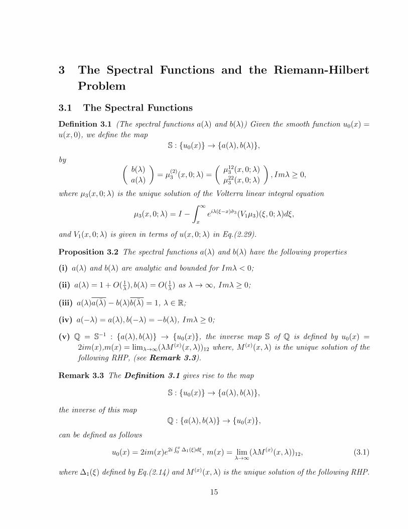
Remark 3.3 The Definition 3.1 gives rise to the map
S : u0(x) → a(λ), b(λ),
the inverse of this map
Q : a(λ), b(λ) → u0(x),
can be defined as follows
u0(x) = 2im(x)e2i∫ x0 ∆1(ξ)dξ, m(x) = lim
λ→∞(λM (x)(x, λ))12, (3.1)
where ∆1(ξ) defined by Eq.(2.14) and M (x)(x, λ) is the unique solution of the following RHP.
15
• M (x)(x, λ) =
M
(x)− (x, λ), λ ∈ D1 ∪D2
M(x)+ (x, λ), λ ∈ D3 ∪D4
is a sectionally meromorphic function.
• M (x)+ (x, λ) = M
(x)− (x, λ)(J (x)(x, λ))−1, λ ∈ R, and
J (x)(x, λ) =
1 b(λ)a(λ)
e−2iλx
− b(λ)
a(λ)e2iλx 1
a(λ)a(λ)
. (3.2)
• M (x)(x, λ) = I +O( 1λ), λ→∞.
• a(λ) has 2n simple zeros εj2n1 , 2n = 2n1 + 2n2, such that, εj(j = 1, 2, · · · , 2n1) lie in
D3 ∪D4, εj(j = 1, 2, · · · , 2n2) lie in D1 ∪D2.
• The first column ofM(x)− (x, λ) has simple poles at λ = εj, j = 1, 2, · · · , 2n2. The second
column of M(x)+ (x, λ) has simple poles at λ = εj, j = 1, 2, · · · , 2n1. The associated
residues are given by
Res[M (x)(x, λ)]1, εj =e2iεjxb(εj)
a(εj)[M (x)(x, εj)]2, j = 1, 2, · · · , 2n2, (3.3)
Res[M (x)(x, λ)]2, εj =e−2iεjxb(εj)
a(εj)[M (x)(x, εj)]1, j = 1, 2, · · · , 2n1. (3.4)
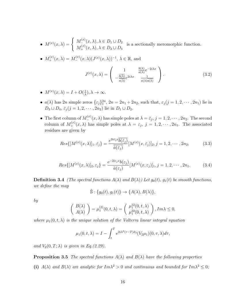
Definition 3.4 (The spectral functions A(λ) and B(λ)) Let g0(t), g1(t) be smooth functions,
we define the map
S : g0(t), g1(t) → A(λ), B(λ),
by (B(λ)
A(λ)
)= µ
(2)1 (0, t, λ) =
(µ12
1 (0, t, λ)
µ221 (0, t, λ)
), Imλ ≤ 0,
where µ1(0, t, λ) is the unique solution of the Volterra linear integral equation
µ1(0, t, λ) = I −∫ T
t
e2iλ2(τ−T )σ3(V2µ1)(0, τ, λ)dτ,
and V2(0, T ;λ) is given in Eq.(2.29).
Proposition 3.5 The spectral functions A(λ) and B(λ) have the following properties
(i) A(λ) and B(λ) are analytic for Imλ2 > 0 and continuous and bounded for Imλ2 ≤ 0;
16
(ii) A(λ) = 1 +O( 1λ), B(λ) = O( 1
λ) as λ→∞, Imλ2 ≤ 0;
(iii) A(λ)A(λ)−B(λ)B(λ) = 1, λ2 ∈ R;
(iv) A(−λ) = A(λ), B(−λ) = −B(λ), Imλ2 ≤ 0;
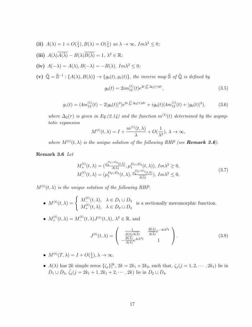
(v) Q = S−1 : A(λ), B(λ) → g0(t), g1(t), the inverse map S of Q is defined by
g0(t) = 2im(1)12 (t)e2i
∫ t0 ∆2(τ)dτ , (3.5)
g1(t) = (4m(1)12 (t)− 2|g0(t)|2)e2i
∫ t0 ∆2(τ)dτ + ig0(t)(4m
(1)12 (t) + |g0(t)|2), (3.6)
where ∆2(τ) is given in Eq.(2.14) and the function m(1)(t) determined by the asymp-
totic expansion
M (t)(t, λ) = I +m(1)(t, λ)
λ+O(
1
λ2), λ→∞,
where M (t)(t, λ) is the unique solution of the following RHP (see Remark 3.6).
Remark 3.6 Let
M(t)+ (t, λ) = (
µD1∪D32 (t,λ)
A(λ), µD1∪D3
1 (t, λ)), Imλ2 ≥ 0,
M(t)− (t, λ) = (µD2∪D4
1 (t, λ),µD2∪D42 (t,λ)
A(λ)), Imλ2 ≤ 0,
(3.7)
M (t)(t, λ) is the unique solution of the following RHP.
• M (t)(t, λ) =
M
(t)− (t, λ), λ ∈ D1 ∪D3
M(t)+ (t, λ), λ ∈ D2 ∪D4
is a sectionally meromorphic function.
• M (t)+ (t, λ) = M
(t)− (t, λ)J (t)(t, λ), λ2 ∈ R, and
J (t)(t, λ) =
1
A(λ)A(λ)
B(λ)
A(λ)e−4iλ2t
−B(λ)A(λ)
e4iλ2t 1
. (3.8)
• M (t)(T, λ) = I +O( 1λ), λ→∞.
• A(λ) has 2k simple zeros ζj2k1 , 2k = 2k1 + 2k2, such that, ζj(j = 1, 2, · · · , 2k1) lie in
D1 ∪D3, ζj(j = 2k1 + 1, 2k1 + 2, · · · , 2k) lie in D2 ∪D4.
17

• The first column of M(t)+ (t, λ) has simple poles at λ = ζj, j = 1, 2, · · · , 2k1. The second
column of M(t)− (t, λ) has simple poles at λ = ζj, j = 1, 2, · · · , 2k2.
The associated residues are given by
Res[M (t)(t, λ)]1, ζj =e4iζ2
j t
A(ζj)B(ζj)[M (t)(t, ζj)]2, j = 1, 2, · · · , 2k1, (3.9)
Res[M (t)(t, λ)]2, ζj =e−4iζ2
j t
A(ζj)B(ζj)[M (t)(t, ζj)]1, j = 1, 2, · · · , 2k2. (3.10)
Definition 3.7 (The spectral functions α(λ) and β(λ)) Given the spectral functions
α(λ) = a(λ)A(λ)− b(λ)B(λ), β(λ) = a(λ)B(λ)− b(λ)A(λ),
and the smooth functions hT (x) = u(x, T ). We define the map
˜S : hT (x) → α(λ), β(λ),
by (β(λ)
α(λ)
)= µ
(2)1 (0, T ;λ) =
(µ12
1 (0, T ;λ)
µ221 (0, T ;λ)
), Imλ ≥ 0,
where µ1(x, T ;λ) is the unique solution of the Volterra linear integral equation
µ1(x, T ;λ) = I −∫ x
0
eiλ2(ξ−x)σ3(V1µ1)(ξ, T ;λ)dξ.
Proposition 3.8 The spectral functions α(λ) and β(λ) have the following properties
(i) α(λ) and β(λ) are analytic for Imλ > 0 and continuous and bounded for Imλ ≥ 0;
(ii) α(λ) = 1 +O( 1λ), β(λ) = O( 1
λ) as λ→∞, Imλ ≥ 0;
(iii) α(λ)α(λ)− β(λ)β(λ) = 1, λ ∈ R;
(iv) α(−λ) = α(λ), β(−λ) = −β(λ), Imλ ≥ 0;
(v) ˜Q = ˜S−1
: α(λ), β(λ) → hT (x), the inverse map ˜S of ˜Q is defined by
hT (x) = 2imT (x)e2i∫ x0 ∆1(ξ,T )dξ, mT (x) = lim
λ→∞(λM (T )(x, λ))12, (3.11)
where M (T )(x, λ) is the unique solution of the following RHP (see Remark 3.9).
18
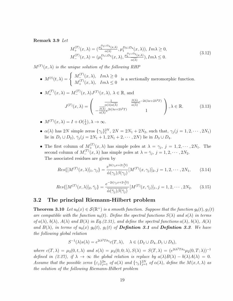
Remark 3.9 Let
M(T )+ (x, λ) = (
µD3∪D43 (x,λ)
α(λ), µD3∪D4
1 (x, λ)), Imλ ≥ 0,
M(T )− (x, λ) = (µD1∪D2
1 (x, λ),µD1∪D23 (x,λ)
α(λ)), Imλ ≤ 0.
(3.12)
M (T )(x, λ) is the unique solution of the following RHP
• M (t)(t, λ) =
M
(T )− (x, λ), Imλ ≥ 0
M(T )+ (x, λ), Imλ ≤ 0
is a sectionally meromorphic function.
• M (T )+ (x, λ) = M
(T )− (x, λ)J (T )(x, λ), λ ∈ R, and
J (T )(x, λ) =
1
α(λ)α(λ)
β(λ)
α(λ)e−2i(λx+2λ2T )
−β(λ)α(λ)
e2i(λx+2λ2T ) 1
, λ ∈ R. (3.13)
• M (T )(x, λ) = I +O( 1λ), λ→∞.
• α(λ) has 2N simple zeros γj2N1 , 2N = 2N1 + 2N2, such that, γj(j = 1, 2, · · · , 2N1)
lie in D1 ∪D2), γj(j = 2N1 + 1, 2N1 + 2, · · · , 2N) lie in D3 ∪D4.
• The first column of M(T )+ (x, λ) has simple poles at λ = γj, j = 1, 2, · · · , 2N1. The
second column of M(T )− (x, λ) has simple poles at λ = γj, j = 1, 2, · · · , 2N2.
The associated residues are given by
Res[M (T )(x, λ)]1, γj =e2i(γjx+2γ2
j t)
α(γj)β(γj)[M (T )(x, γj)]2, j = 1, 2, · · · , 2N1, (3.14)
Res[M (T )(x, λ)]2, γj =e−2i(γjx+2γ2
j t)
α(γj)β(γj)[M (T )(x, γj)]1, j = 1, 2, · · · , 2N2. (3.15)
3.2 The principal Riemann-Hilbert problem
Theorem 3.10 Let u0(x) ∈ S(R+) is a smooth function. Suppose that the function g0(t), g1(t)
are compatible with the function u0(t). Define the spectral functions S(λ) and s(λ) in terms
of a(λ), b(λ), A(λ) and B(λ) in Eq.(2.31), and define the spectral functions a(λ), b(λ), A(λ)
and B(λ), in terms of u0(x) g0(t), g1(t) of Defintion 3.1 and Defintion 3.3. We have
the following global relation
S−1(λ)s(λ) = e2iλ2T σ3c(T, λ), λ ∈ (D2 ∪D4, D1 ∪D3),
where c(T, λ) = µ3(0, t, λ) and s(λ) = µ3(0, 0;λ), S(λ) = S(T, λ) = (e2iλ2T σ3µ2(0, T ;λ))−1
defined in (2.27), if λ → ∞ the global relation is replace by a(λ)B(λ) − b(λ)A(λ) = 0.
Assume that the possible zeros εj2nj=1 of a(λ) and γj2N
j=1 of α(λ), define the M(x, t, λ) as
the solution of the following Riemann-Hilbert problem
19
• M(x, t;λ) is a sectionally meromorphic on the Riemann λ-sphere with jumps across
the contours on Dn ∩ Dm(n,m = 1, 2, 3, 4) (see figure 2).
• M(x, t;λ) satisfies the jump condition with jumps across the contours on Dn∩Dm(n,m =
1, 2, 3, 4)
M+(x, t;λ) = M−(x, t;λ)J(x, t;λ), λ ∈ Dn ∩ Dm, n,m = 1, 2, 3, 4;n 6= m. (3.16)
• M(x, t;λ) = I +O( 1λ), λ→∞.
• The residue condition of M(x, t;λ) is showed in Proposition 2.6.
Then M(x, t;λ) exists and is unique, we define u(x, t) in terms of M(x, t;λ) by
u(x, t) = 2im(x, t)e2i∫ (x,t)(0,0)
∆,
m(x, t) = limλ→∞(λM(x, t;λ))12,
∆ = 4|m|2dx+ (48|m|4 − 4i(mxm−mxm))dt.
(3.17)
Furthermore, under the defined that the initial values u(x, 0) = u0(x) and boundary values
u(0, t) = g0(t), ux(0, t) = g1(t) lie in the Schwartz space, u(x, t) is the solution of the KE
equation (1.1).
Proof. In fact, if a(λ) and α(λ) have no zeroes, then the 2 × 2 function M(x, t;λ)
satisfies a non-sigular RHP. Using the fact that the jump matrix J(x, t;λ) match with the
symmetry conditions, we can show that this problem has a unique global solution [47]. The
case that a(λ) and α(λ) have a finite number of zeros can be mapped to the case of no zeros
supplemented by an algebraic system of equations which is always uniquely solvable.
Therefore, similar to the reference [13], we have the following vanishing theorem hold
true.
Theorem 3.11 The RHP in Theorem 3.10 with the vanishing boundary condition M(x, t;λ)→0 (λ→∞), has only the zero solution.
Proof Suppose that M(x, t;λ) is a solution of the RHP in Theorem 3.10 such that
M±(x, t;λ) → ∞ (λ → ∞). Let A is a 2 × 2 matrix, A†denote the complex conjugate
transpose of A. Define
H+(λ) = M+(λ)M †−(−λ), Imλ2 ≥ 0,
H−(λ) = M−(λ)M †+(−λ), Imλ2 ≤ 0,
(3.18)
where the x and t are dependence. H+(λ) and H−(λ) is analytic in λ ∈ C\ Imλ2 > 0 and
λ ∈ C \ Imλ2 < 0, respectively. By the symmetry relations a(−λ) = a(λ), b(−λ) = −b(λ),
and A(−λ) = A(λ), B(−λ) = −B(λ) in Proposition 2.3 and Eq.(2.36), we have
J†1(−λ) = J1(λ), J†3(−λ) = J3(λ), J†2(−λ) = J4(λ). (3.19)
20
ThenH+(λ) = M−(λ)J(λ)M †
−(−λ), Imλ2 ∈ R,H−(λ) = M−(λ)J†(−λ)M †
−(−λ), , Imλ2 ∈ R.(3.20)
It is not difficult to see that H+(λ) = H−(λ) for Imλ2 ∈ R. Therefore, H+(λ) and H−(λ)
define an entire function vanishing at infinity, so H+(λ) and H−(λ) are identically zero.
Noting J3(iκ)(κ ∈ R), is a Hermitian matrix with unit determinant and (2, 2) entry 1 for
any κ ∈ R. Therefore, J3(iκ)(κ ∈ R) is a positive definite matrix. Since H−(κ) vanishes
identically for κ ∈ iR, i.e.
M+(iκ)J3(iκ)M †+(iκ) = 0, κ ∈ R. (3.21)
We can infer that M+(iκ) = 0 as κ ∈ R. It follows that M+(λ) and M−(λ) vanish identically.
Remark 3.12 Proof that u(x, t) satisfies the KE equation.
Using arguments of the dressing method [48], it can be verified directly that if u(x, t) is
defined in terms of M(x, t;λ) by Eq.(3.17), and if M(x, t;λ) is defined as the unique solution
of the above RHP, then u(x, t) and M(x, t;λ) satisfy two parts of the Lax pair, hence u(x, t)
is solvable on KE equation.
Remark 3.13 We can use similar method with [11] to prove that initial values u(x, 0) =
u0(x) and boundary values u(0, t) = g0(t), ux(0, t) = g1(t), we omit this proof in here because
of the length of this article.
4 Conclusions and discussions
In this paper, we consider IBV of the KE equation on the half-line. Using the Fokas unified
transform method for nonlinear evolution systems which taking the form of Lax pair isospec-
tral deformations and whose corresponding continuous spectra Lax operators, assume that
the solution u(x, t) exists, we show that it can be represented in terms of the solution of a
matrix Riemann-Hilbert problem formulated in the plane of the complex spectral parameter
λ. The jump matrix has explicit (x, t) dependence and is given in terms of the spectral
functions a(λ), b(λ) and A(λ), B(λ), which obtained from the initial data u0(x) = u(x, 0)
and the boundary data g0(t) = u(0, t), g1(t) = ux(0, t), respectively. The spectral functions
are not independent, but related by a compatibility condition, the so-called global relation.
For other integrable equations, can we construct their solution of a matrix Riemann-Hilbert
problem formulated in the plane of the complex spectral parameter λ by the similar method?
In paper [12], Xiao and Fan obtained the soliton-type solutions of the Harry-Dym equation
by solving the particular Riemann-Hilbert problem with vanishing scattering coefficients,
21
can we obtain the soliton-type solutions of the KE equation following the same ways? More-
over, Zhu have successfully applied the Deift-Zhou nonlinear steepest descent method to
analyzed the long-time asymptotic for the solutions of decay initial value problem of the KE
equation in [46]. But under the assumption that the initial and boundary values lie in the
Schwartz class, can we do the long-time asymptotics for the solutions of the decay initial
and boundary values of KE equation following the same ways as for the derivative nonlinear
Schrodinger equation [49] and Fokas-Lenells equation [50]? These three questions will be
discussed in our future work.
Acknowledgements
This work is partially supported by the National Natural Science Foundation of China under
Grant Nos. 12271008 and 11601055, Natural Science Foundation of Anhui Province under
Grant No.1408085QA06.
References
[1] A. S. Fokas, A unified transform method for solving linear and certain nonlinear PDEs, Proc.
R. Soc. Lond. A 453 (1997) 1411-1443.
[2] A. S. Fokas, Integrable nonlinear evolution equations on the half-line, Commun. Math. Phys.
230 (2002) 1-39.
[3] A. S. Fokas, A unified approach to boundary value problems. CBMS-NSF Regional Con-
ference Series in Applied Mathematics. Philadelphia, PA: Society of Industrial and Applied
Mathematics. (2008)
[4] A. Boutet de Monvel, A. S. Fokas, D. Shepelsky, The mKDV equation on the half-line, J.
Inst. Math. Jussieu. 3 (2004) 139-164.
[5] A. S. Fokas, A. R. Its, L. Y. Sung, The nonlinear Schrodinger equation on the half-line,
Nonlinearity 18 (2005) 1771-1822.
[6] A. Boutet de Monvel, A. S. Fokas, D. Shepelsky, Integrable nonlinear evolution equations on
a finite interval, Comm. Math. Phys. 263 (2006) 133-172.
[7] B. Pelloni, D. A Pinotsis, The Klein-Gordon Equation on the Half Line: a Riemann-Hilbert
Approach. Journal of Nonlinear Mathematical Physics 15 (2008) 334-336.
[8] J. Lenells, The derivative nonlinear Schrodinger equation on the half-line, Physica D 237
(2008) 3008-3019.
[9] J. Lenells, A. S. Fokas, Boundary-value problems for the stationary axisymmetric Einstein
equations: a rotating disc. Nonlinearity 24 (2011) 177-206.
22
[10] J. Lenells, Boundary value problems for the stationary axisymmetric Einstein equations: a
disk rotating around a black hole, Comm. Math. Phys. 304 (2011) 585-635.
[11] J. Xu, E. G. Fan, A Riemann-Hilbert approach to the initial-boundary problem for derivative
nonlinear Schrodinger equation. Acta Math. Sci. Ser. B Engl. Ed. 34 (4) (2014) 973-994.
[12] Y. Xiao, E. G. Fan, A Riemann-Hilbert approach to the Harry-Dym equation on the line,
Chinese Annals of Mathematics, Series B 37 (3) (2016) 373-384.
[13] N. Zhang, T. C. Xia, B. B. Hu, A Riemann-Hilbert Approach to the Complex Sharma-Tasso-
Olver Equation on the Half Line, Commun. Theor. Phys. 68 (2017) 580-594.
[14] B. Q. Xia, A. S. Fokas, Initial-boundary value problems associated with the Ablowitz-Ladik
system, (2017) Arxiv ID: 1703.01687
[15] B. Deconinck, Q. Guo, E. Shlizerman, V. Vasan, Fokas’s Unified Transform Method for linear
systems, (2017) Arxiv ID: 1705.00358
[16] J. Lenells, Initial-boundary value problems for integrable evolution equations with 3× 3 Lax
pairs, Phys. D 241(2012),857.
[17] J. Lenells, The Degasperis-Procesi equation on the half-line, Nonlinear Anal 76 (2013) 122.
[18] A. Boutet de Monvel, D. Shepelsky, A Riemann-Hilbert approach for the Degasperis-Procesi
equation, Nonlinearity 26 (2013) 2081.
[19] J. Xu, E. G. Fan, The unified method for the Sasa-Satsuma equation on the half-line, Proc.
R. Soc. A, Math. Phys. Eng. Sci. 469 (2013),1.
[20] J. Xu, E. G. Fan, The three wave equation on the half-line, Phys. Lett. A 378 (2014) 26.
[21] X. G. Geng, H. Liu, J. Y. Zhu. Initial-boundary value problems for the coupled nonlinear
Schrodinger equation on the half-line, Stud. Appl. Math. 135 (2015) 310.
[22] H. Liu, X. G. Geng, Initial-boundary problems for the vector modified Korteweg-deVries
equation via Fokas unified transform method, J. Math. Anal. Appl. 440 (2016) 578.
[23] A. Boutet de Monvel, D. Shepelsky, L. Zielinski, A Riemann-Hilbert approach for the Novikov
equation, SIGMA 12 (2016) 095.
[24] S. F. Tian, Initial-boundary value problems for the general coupled nonlinear Schrodinger
equation on the interval via theFokas method. Journal of Differential Equations, 262(1) (2017)
506-558.
[25] Z. Y. Yan, An initial-boundary value problem for the integrable spin-1 Gross-Pitaevskii equa-
tions with a 4× 4 Lax pair on the half-line, CHAOS 27 (2017) 053117.
[26] B. B. Hu, T. C. Xia, Initial-boundary value problems for the coupled higher-order nonlin-
ear Schrodinger equations on the half-line. International Journal of Nonlinear Sciences and
Numerical Simulation, Accepted.
[27] B. B. Hu, T. C. Xia, The coupled modified nonlinear Schrodinger equations on the half-line
via the Fokas method, (2017) Arxiv ID: 1704.03623
23
[28] P. Deift, X. Zhou, A steepest descent method for oscillatory Riemann-Hilbert problems, Ann.
Math. 137 (1993) 295-368.
[29] A.Kundu, Landau-Lifshitz and higher-order nonlinear systems gauge generated from nonlinear
Schrodinger-type equations, J. Math. Phys. 25 (1984) 3433-3438.
[30] F. Calogero, W. Eckhaus, Nonlinear evolution equations, rescalings, model PDEs and their
integrability, I. Inverse Probl. 3 (1987) 229-262.
[31] P. A. Clarkson, C. M. Cosgrove, Painleve analysis of the nonlinear Schrodinger family of
equations, J. Phys. A Math. Gen. 20 (1987) 2003-2024.
[32] X. G. Geng, A hierarchy of non-linear evolution equations, its Hamiltonian structure and
classical integrable system, Phys. A 80 (1992) 241-251.
[33] A. Kundu, Integrable hierarchy of higher nonlinear Schrodinger type equations, Symmetry
Integrability Geom. Methods Appl. 2 (2006) 078.
[34] D. Levi, C. Scimiterna, The Kundu-Eckhaus equation and its discretizations, J. Phys. A:
Math. Theor. 42 (2009) 465203.
[35] X. Lu, M. S. Peng, Systematic construction of infinitely many conservation laws for certain
nonlinear evolution equations inmathematical physics, Commun. Nonlinear Sci. Numer. Sim-
ulat. 18 (2013) 2304-2312.
[36] S. Kakei, N. Sasa, J. Satsuma, Bilinearization of a generalized derivative nonlinear Schrodinger
equation, J. Phys. Soc. Jpn 64 (1995) 1519-1523.
[37] X. G. Geng, H. W. Tam, Darboux transformation and soliton solutions for generalized non-
linear Schrodinger equations, J. Phys. Soc. Jpn 68 (1999) 1508-1512.
[38] Z. Feng, X. Wang, Explicit exact solitary wave solutions for the Kundu equation and the
derivative Schrodinger equation. Phys. Scr. 64 (2001) 7-14.
[39] P. Wang, B. Tian, K. Sun, F. H. Qi, Bright and dark soliton solutions and Backlund transfor-
mation for the Eckhaus-Kundu equation with the cubic-quintic nonlinearity, Applied Mathe-
matics and Computation 251 (2015) 233-242.
[40] H. M. Baskonus, H. Bulut, On the complex structures of Kundu-Eckhaus equation via im-
proved Bernoulli sub-equation function method, Waves in Random and Complex Media 25
(4) (2015) 720-728.
[41] Q. L. Zha, On Nth-order rogue wave solution to the generalized nonlinear Schrodinger equa-
tion, Phys. Lett. A 377 (2013) 855-859.
[42] X. Wang, B. Yang, Y. Chen, Y. Q. Yang, Higher-order rogue wave solutions of the Kundu-
Eckhaus equation, Phys. Scr. 89 (2014) 095210.
[43] D. Q. Qiu, J. S. He, Y. S. Zhang, K. Porsezian The Darboux transformation of the Kundu-
Eckhaus equation, Proc. R. Soc. A 471 (2015) 20150236.
24
[44] X. Y. Xie, B. Tian, W. R. Sun, Y. Sun, Rogue-wave solutions for the Kundu-Eckhaus equation
with variable coefficients in an optical fiber, Nonlinear Dynamics 81 (3) (2015) 1349-1354.
[45] C. Bayındır, Rogue wave spectra of the Kundu-Eckhaus equation, Physical Review E 93
(2016) 062215.
[46] Q. Z. Zhu, J. Xu, E. G. Fan, The Riemann-Hilbert problem and long-time asymptotics for the
Kundu-Eckhaus equation with decaying initial value, Applied Mathematics Letters 76 (2018)
81-89.
[47] V. E. Adler, B. Gurel, M. Gurses, I. Habibullin, Boundary conditions for integrable equations,
J. Phys. A 30 (1997) 3505-3513.
[48] V. E. Zakharov, A. Shabat, A scheme for integrating the nonlinear equations of mathematical
physics by the method of the inverse scattering problem, I and II, Funct. Anal. Appl. 8 (1974)
226-235 and 13 (1979) 166-174.
[49] L. K. Arruda, J. Lenells, Long-time asymptotics for the derivative nonlinear Schrodinger
equation on the half-line, (2017) Arxiv ID: 1702.02084
[50] S. Y. Chen, Z. Y. Yan, Long-time asymptotics for initial-boundary value problems of integrable
Fokas-Lenells equation on the half-line, (2017) Arxiv ID: 1710.06563
25