Journal of Multivariate Analysis 124 (2014) 116–129

Contents lists available at ScienceDirect

Journal of Multivariate Analysis

journal homepage: www.elsevier.com/locate/jmva

A revisit to correlation analysis for distortion measurementerror data

Jun Zhang a, Zhenghui Feng b,∗, Bu Zhou c

a Shen Zhen-Hong Kong Joint Research Centre for Applied Statistical Sciences, College of Mathematics and Computational Science,Shenzhen University, Shenzhen, Chinab The Wang Yanan Institute for Studies in Economics, The School of Economics, Xiamen University, Xiamen, Chinac Department of Statistics and Applied Probability, National University of Singapore, Singapore

a r t i c l e i n f o

Article history:Received 10 January 2013Available online 31 October 2013

AMS subject classifications:62G0862G2062F12

Keywords:Correlation coefficientDistorting functionMeasurement error modelsKernel smoothing

a b s t r a c t

In this paper, we consider the estimation problem of a correlation coefficient betweenunobserved variables of interest. These unobservable variables are distorted in a multi-plicative fashion by an observed confounding variable. Two estimators, themoment-basedestimator and the direct plug-in estimator, are proposed, and we show their asymptoticnormality. Moreover, the direct plug-in estimator is shown asymptotically efficient. Fur-thermore, we suggest a bootstrap procedure and an empirical likelihood-based statistic toconstruct the confidence interval. The empirical likelihood statistic is shown to be asymp-totically chi-squared. Simulation studies are conducted to examine the performance of theproposed estimators. These methods are applied to analyze the Boston housing price dataas an illustration.

© 2013 Elsevier Inc. All rights reserved.

1. Introduction

Measurement error is common in many disciplines, such as economics, health science and medical research, due to im-proper instrument calibration ormany other reasons. Generally, an estimation procedurewhich ignoresmeasurement errormay cause large bias, sometimes seriously large bias. The classical statistical estimation and inference become very challeng-ing. Therefore, it requires particular care to eliminate such bias when estimating target parameters. Research on classicalerrors-in-variables have been widely studied in the last two decades, for example by Li and Hsiao [12] and Schennach [26]using replicate data, and Carroll et al. [37], Schennach [27] and Wang and Hsiao [3], using instrumental variable methods.Others considered nonparametric or semi-parametric approaches (Carroll et al. [25]; Delaigle et al. [36]; Liang et al. [46];Liang and Li [17]; Liang andRen [19]; Liang andWang [20]; Schafer [16], Taupin [1]; Zhou and Liang [6]). In addition, Fuller [9]and Carroll et al. [4] give comprehensive reviews containing many parametric and semi-parametric measurement errormodels.

In this paper, we consider multiplicative effect type errors, namely, distorting measurement errors. Both the responseand predictors are unobservable and distorted by general multiplicative effects of some observable confounding variable as

Y = φ(U)Y ,X = ψ(U)X,

(1.1)

∗ Corresponding author.E-mail addresses: zhangjunstat@gmail.com (J. Zhang), zhfengwise@gmail.com (Z. Feng), zhoubu1988@163.com (B. Zhou).

0047-259X/$ – see front matter© 2013 Elsevier Inc. All rights reserved.http://dx.doi.org/10.1016/j.jmva.2013.10.004

J. Zhang et al. / Journal of Multivariate Analysis 124 (2014) 116–129 117

where (Y , X)τ are the unobservable continuous variables of interest, (the superscript τ denotes the transpose operatorthroughout this paper), while (Y , X)τ are available distorted variables. φ(·) andψ(·) are unknown contaminating functionsof an observed confounding variable U , and U is independent of (X, Y )τ .

The distortionmeasurement errorsmodel (1.1) usually occurs in biomedical and health-related studies. The confoundingvariable (for example, it can be the bodymass index (BMI), height orweight) usually has some kind ofmultiplicative effect onthe primary variables of interest. Kaysen et al. [11] analyzed the relationship between fibrinogen level and serum transferrinlevel among hemodialysis patients, and realized that BMI plays the role of confounding variable that may contaminate thefibrinogen level and the serum transferrin level simultaneously. To eliminate the potential bias, Kaysen et al. [11] simplydivided the observed fibrinogen level-Y and observed serum transferrin level-X by BMI-U . Şentürk and Müller [30] noticedthat the exact relationship between the confounding variable (BMI) and primary variables is hardly known in practice. Sucha simple way of dividing confounding variable BMI may not be appropriate and may lead to an inconsistent estimator ofthe target parameters. So Şentürk andMüller [30] proposedmodel (1.1) as a flexible multiplicative adjustment by involvingunknown smooth distorting functions φ(·), ψ(·) for the confounding variable U .

To estimate the correlation coefficient between Y and X , denoted as ρ(Y ,X), Şentürk andMüller [28] observed that the di-rect calculation of correlation coefficient between Y and X will result in an arbitrarily large biased estimator of ρ(Y ,X). There-fore, a proper adjustmentmethod for estimating ρ(Y ,X) needs to be addressed. To solve this problem, Şentürk andMüller [28]established the relationship between Y and X through a varying coefficientmodel, and then employed the binning techniqueto estimate ρ(Y ,X). Such a transformation procedure can be generalized to regression models with linear structure—for ex-ample, linear models [28,30,22,21], generalized linear models [31] and partial linear single index models [43].

The goal of this paper is to construct consistent estimation and do inference for correlation coefficient ρ(Y ,X). Twoestimators for ρ(Y ,X) are proposed. One is the moment-based estimator, and the other is the direct plug-in estimator. Thebasic ideas and motivations of these two methods are summarized as follows.

• Our first estimator is based on ρ(Y ,X) = ρ(eYU ,eXU )/∆ for some unknown constant ∆, where ρ(eYU ,eXU ) is the correlation

coefficient between eYU = Y − E[Y |U] and eXU = X − E[X |U], i.e., ρ(eYU ,eXU ) =Cov(eYU ,eXU )√Var(eYU )Var(eXU )

in the population level.

This relationshipρ(Y ,X) = ρ(eYU ,eXU )/∆was first revealed in Appendix D of Şentürk andMüller [28], but they did not study

the statistical properties and simulations further. However, ρ(Y ,X) = ρ(eYU ,eXU )/∆ implies that ρ(eYU ,eXU )/∆ is also an es-

timator of ρ(Y ,X), where ρ(eYU ,eXU ) and ∆ are some estimators of ρ(eYU ,eXU ) and∆, respectively. So it is worth studying theestimation procedure for ρ(eYU ,eXU )/∆ and its associated sample properties. We propose moment-based estimators forρ(eYU ,eXU )

,∆ and further establish their asymptotic normality properties. Moreover, some simulations are also evaluated.To construct a confidence interval for ρ(Y ,X), a wild bootstrap procedure is proposed.

• The second estimator is based on the recent methodology direct plug-in, proposed by Cui et al. [5]. The direct plug-inmethod is a convenient tool for distorting measurement error data. The basic idea is to obtain estimators of the distor-tion functions, say φ, ψ and then calibrate Y and X by Y/φ, X/ψ , and finally construct estimation by using these cali-brated quantities. The direct plug-in method can be easily adopted in parametric and semi-parametric models, see forinstance [5,45,44,13,42]. In this paper, an estimator of ρ(Y ,X) based on the direct plug-in method is also investigated. Aninteresting result is that the direct plug-in estimator for ρ(Y ,X) is efficient, i.e., the asymptotic variance of the direct plug-inestimator is the same as the classical asymptotic variance of the sample correlation coefficient (see for example [8], Sec-tion 8) when data has no distortion effect (φ(·) ≡ 1, ψ(·) ≡ 1). In other words, this direct plug-in estimation procedurefor ρ(Y ,X) eliminates the effect caused by the multiplying distorting measurement error φ(U), and ψ(U). Moreover, anempirical likelihood-based statistic is proposed to construct a confidence interval.

Further, we use our proposed estimators to re-analyze Boston housing price data. In [28], the authors used the educationlevel ‘Lstat’ as the confounding variable to investigate the correlation between ‘Crime’ and ‘price’. Zhang et al. [45] indicatedthat another choice of confounding variable is ‘Ptratio’, pupil–teacher ratio by town. We will make a comparison for thoseestimators of ρ(Y ,X) under these two different choices of confounding variables to see which estimator is more informativeand reasonable.

The paper is organized as follows. In Section 2, we propose the moment-based estimator and derive related asymptoticresults. A wild bootstrap procedure to construct a confidence interval is also investigated. In Section 3, we give the directplug-in estimator and present some asymptotic results. We develop a calibrated empirical log-likelihood ratio statistic andshow that the statistic has an asymptotic chi-squared distribution. In Section 4, simulation studies are conducted to examinethe performance of the proposed methods. In Section 5, the analysis of Boston housing price data is presented. All technicalproofs of the asymptotic results are given in the Supplementary material.

2. Estimation procedure and asymptotic results

To ensure identifiability for model (1.1), Şentürk and Müller [28] introduced that

E[φ(U)] = 1, E[ψ(U)] = 1. (2.2)

118 J. Zhang et al. / Journal of Multivariate Analysis 124 (2014) 116–129

This assumption is similar to that of classical measurement error, for instance, the common assumption E(e) = 0 forW = X + e, whereW is error-prone and X is error-free. Together with (1.1) and (2.2), we have

E[Y |U] = φ(U)E[Y |U] = φ(U)E[Y ],

E[X |U] = ψ(U)E[X |U] = ψ(U)E[X].(2.3)

Define eYU = Y − E[Y |U] = Y − φ(U)E[Y ] and eXU = X − E[X |U] = X − ψ(U)E[X]. Under (1.1), (2.2) and (2.3), Şentürkand Müller [28] proved that

ρ(eYU ,eXU )=

Cov(eYU , eXU)σ 2eYUσ 2eXU

= ρ(Y ,X)E[φ(U)ψ(U)]

E[φ2(U)]E[ψ2(U)]def= ρ(Y ,X)∆, (2.4)

where σ 2eYU

= Var(eYU) and σ2eXU

= Var(eXU)—for more details see Appendix D of [28], which indicated that ∆ can be anyvalue in (0, 1] under some mild conditions. From (2.4), Pearson’s correlation coefficient ρ(Y ,X) can be directly estimated byρ(Y ,X) = ρ(eYU ,eXU )

/∆ in the population level. Thus, a new estimation procedure can be constructed by using an estimator ofPearson’s correlation coefficient ρ(eYU ,eXU ) between (eYU , eXU), together with an estimator of the unknown constant ∆. Wedescribe the procedures in the following subsections.

2.1. Estimating procedure and asymptotic result for ρ(eYU ,eXU )

In (2.4), a moment-based estimation procedure for ρ(eYU ,eXU ) can be constructed by estimating Cov(eYU , eXU), σ2eYU

and

σ 2eXU

respectively. We propose our estimators as

Cov(eYU , eXU) = n−1n

i=1

eiYU eiXU − ¯eYU ¯eXU , (2.5)

σ 2eYU

= n−1n

i=1

e2iYU

− [¯eYU ]2, (2.6)

σ 2eXU

= n−1n

i=1

e2iXU

− [¯eXU ]2, (2.7)

where ¯eYU = n−1 ni=1 eiYU , ¯eXU = n−1 n

i=1 eiXU with eiYU = Yi −Eh(Yi|Ui), eiXU = Xi −Eh(Xi|Ui).Eh(Yi|Ui),Eh(Xi|Ui) arethe Nadaraya–Watson estimators for E(Yi|Ui) and E(Xi|Ui), which are defined as

Eh(Yi|Ui) =

n−1n

j=1Kh(Uj − Ui)Yj

n−1n

j=1Kh(Uj − Ui)

, Eh(Xi|Ui) =

n−1n

j=1Kh(Uj − Ui)Xj

n−1n

j=1Kh(Uj − Ui)

. (2.8)

Here Kh(·) = h−1K(·/h), and K(·) denotes a kernel density, h is a positive-valued bandwidth. Using (2.5)–(2.7), the estimatorof ρ(eYU ,eXU ) can be defined as

ρ(eYU ,eXU )=

Cov(eYU , eXU)σ 2eYUσ 2eXU

. (2.9)

We have the following asymptotic result.

Theorem 1. Under Conditions (A1)–(A4), and (A5)(i) given in Appendix A, we have√n

ρ(eYU ,eXU )

− ρ(eYU ,eXU )

L

−→ N0, σ 2

0

,

where the explicit form of σ 20 is given in the Supplementary material.

Remark 1. If ∆ = 1, i.e., the Cauchy–Schwarz inequality entails that P(φ(U) = cψ(U)) = 1 for some nonzero constantc , it is easy to see that c = 1, due to the identifiability condition (2.2). When ∆ = 1, we have ρ(eYU ,eXU ) = ρ(Y ,X), whichmeans that ρ(eYU ,eXU ) is also a root-n consistent estimator of ρ(Y ,X) when φ(u) = ψ(u). Moreover, the asymptotic variance

σ 20 can then be reduced to a simple form E[φ4(U)]

{E[φ2(U)]}2σ 2ρ , where σ 2

ρ is the classical asymptotic variance of the sample correlation

J. Zhang et al. / Journal of Multivariate Analysis 124 (2014) 116–129 119

coefficient (see, for example, [8, Section 8]) when the data are observed without distortion. The distorting factor E[φ4(U)]{E[φ2(U)]}2

is usually greater than one if φ(u) ≡ 1, which means that the distorting functions φ,ψ increase the asymptotic variance.

Remark 2. The condition (A5)(i) shows an under-smoothing approach that is unnecessary to achieve the root-n consistencyof ρ(eYU ,eXU ). Technically speaking, the bandwidth h in Assumption (A5)(i) contains the rate n−1/5 of the ‘optimal’ bandwidth.Thus, most bandwidth selection methods can be employed here, such as the cross-validation method and the plug-inmethod.

2.2. Estimating procedures and asymptotic results for∆ and ρ(Y ,X)

We first propose the estimator for∆. Note that

E[φ(U)ψ(U)] = E[{φ(U)− 1}{ψ(U)− 1}] + 1, (2.10)

E[φ2(U)] = E[{φ(U)− 1}2] + 1, E[ψ2(U)] = E[{ψ(U)− 1}2] + 1. (2.11)

Moreover, (2.3) and the identifiability condition (2.2) entail that φ(U) =E[Y |U]

E[Y ]=

E[Y |U]

E[Y ], ψ(U) =

E[X |U]

E[X]=

E[X |U]

E[X]. Directly

using (2.8), it is easily seen that

φ(Ui) =

Eh1(Yi|Ui)

¯Y, ψ(Ui) =

Eh1(Xi|Ui)

¯X, (2.12)

where ¯Y =1n

ni=1 Yi,

¯X =1n

ni=1 Xi. In (2.12), we choose another bandwidth h1, a different bandwidth from h used in

(2.8). This is because, in Theorem 2, under-smoothing for h1 is needed such that the bias of ∆ is small and the asymptoticnormality of ∆ can be obtained. Together with (2.10)–(2.12), we have

E[φ(U)ψ(U)] = n−1n

i=1

[φ(Ui)− 1][ψ(Ui)− 1] + 1, (2.13)

E[φ2(U)] = n−1n

i=1

[φ(Ui)− 1]2 + 1, E[ψ2(U)] = n−1n

i=1

[ψ(Ui)− 1]2 + 1. (2.14)

Thus, from (2.12)–(2.14), the estimator of∆ can be defined as

∆ =

E[φ(U)ψ(U)]E[φ2(U)]E[ψ2(U)]. (2.15)

Together with (2.9) and (2.15), our target estimator for ρ(Y ,X) can be constructed as

ρ(Y ,X) = ρ(eYU ,eXU )/∆. (2.16)

We have the following asymptotic results.

Theorem 2. Under Conditions (A1)–(A4), and (A5)(ii) in Appendix A,√n

∆−∆

L

−→ N0, σ 2

∆

,

where σ 2∆ = ~1 + ~2∆

2− ~3∆, and the explicit forms of ~i, i = 1, 2, 3, are given in the Supplementary material.

Remark 3. As noted in Remark 1, if ∆ = 1, we can use ρ(eYU ,eXU ) as an estimator of ρ(Y ,X). In this context, the asymptotic

variance of ∆ can be reduced to1 −

1E[φ2(U)]

2, and (2.14) can be directly used as a moment-based estimator of E[φ2(U)].

As a result, a test statistic can be constructed as√n(∆−1)

|1−1/E[φ2(U)]|to test whether∆ = 1 or not.

In (2.4),wemayneed to checkwhether∆ is zero or not in some cases. If∆ ≈ 0 to some extent, the estimator (2.16) cannotbe used to estimate ρ(Y ,X) as the denominator ∆ in (2.16) is close to zero. Generally, we can use Theorem 2 to construct a teststatistic

√n∆/

~1 to test H0 : ∆ = 0, where ~1 is a plug-in consistent estimator of ~1. Nevertheless, ∆ = 0 is equivalent

to E[ψ(U)φ(U)] = 0. Corollary 1 in the following presents an asymptotic normality for estimatorE[φ(U)ψ(U)], which canbe used to test H0 : E [φ(U)ψ(U)] = 0 (or equivalently∆ = 0). See more discussions in the Supplementary material.

120 J. Zhang et al. / Journal of Multivariate Analysis 124 (2014) 116–129

Corollary 1. Under Conditions (A1)–(A4), and (A5)(ii) in Appendix A,√n

E[φ(U)ψ(U)] − E[φ(U)ψ(U)] L

−→ N(0, σ 22 ),

where the explicit form of σ 22 is given in the Supplementary material.

Next, we present the asymptotic normality of the moment-based estimator ρ(Y ,X) in (2.16).

Theorem 3. Under Conditions (A1)–(A5) in Appendix A, we have that√n

ρ(Y ,X) − ρ(Y ,X)

L−→ N

0, σ 2

1

,

where σ 21 = ∆−2σ 2

0 +∆−2ρ2(Y ,X)σ

2∆−Γρ(Y ,X) , σ

20 is the asymptotic variance obtained in Theorem 1, σ 2

∆ is the asymptotic varianceobtained in Theorem 2, and Γρ(Y ,X) is given in the Supplementary material.

Remark 4. From (2.16), it is easily seen that the asymptotic variance of ρ(Y ,X) can be obtained from√n

ρ(Y ,X) − ρ(Y ,X)

=

∆−1√nρ(eYU ,eXU )

− ρ(eYU ,eXU )

−∆−1ρ(Y ,X)

√n∆−∆

+oP(1). Thus, the first term in asymptotic variance σ 2

1 ,∆−2σ 2

0 , can

be viewed as the variance from the first stage estimation of ρ(eYU ,eXU ), the second term ∆−2ρ2(Y ,X)σ

2∆ is the variance of the

second stage for estimating∆, and the third one Γρ(Y ,X) is the covariance of two-stage estimators.

2.3. Constructing bootstrap confidence intervals

In this section, a simple procedure is designed to construct confidence intervals—although we could use ρ(Y ,X) ± zα/2σ1√n

to construct a confidence interval, where zα/2 stands for the (1 − α/2)th quantile of the standard Gaussian distribution. Asthe asymptotic variances obtained in Theorems 1 and 3 are very complex, the finite-sample estimator σ1 for σ1 will certainlyhave an effect on the behavior of confidence intervals, which may not be precise in finite samples. Another problem is thatthe normal approximation confidence intervals may produce unreasonable upper or lower bound. For example, if the truevalue ρ(Y ,X) = 0.9, the upper bound of the interval, ρ(Y ,X)+ zα/2

σ1√n , may be possibly beyond 1. To overcome these problems,

we propose a wild bootstrap [40,33,7] technique to mimic the distribution of the statistic ρ(Y ,X).Step 1: Generate B times i.i.d. variables ςib, i = 1, . . . , n, b = 1, . . . , B with a Bernoulli distribution which respectively

take values at 1∓√5

2 with probability 5±√5

10 . For each b, calculate these arguments e(b)iYU

= ςibeiYU , e(b)iXU

= ςibeiXU and

ρ(ςbeYU ,ςbeXU )=

Cov(ςbeYU , ςbeXU)σ 2ςbeYU

σ 2ςbeXU

, (2.17)

where Cov(ςbeYU , ςbeXU) = n−1 ni=1 e

(b)iYU

e(b)iXU

− ¯e(b)YU

¯e(b)XU , σ

2ςbeYU

= n−1 ni=1[e

(b)iYU

]2−[¯e

(b)YU ]

2 and σ 2ςbeXU

= n−1 ni=1

[e(b)iXU

]2− [¯e

(b)XU ]

2 with ¯e(b)YU = n−1 n

i=1 ςibeiYU , ¯e(b)XU = n−1 n

i=1 ςibeiXU .Step 2: Generate another B times i.i.d. variables ιib, i = 1, . . . , n, b = 1, . . . , B with a Bernoulli distribution which respec-

tively take values at 1∓√5

2 with probability 5±√5

10 . For each b, compute the arguments

∆b =

E(b)[φ(U)ψ(U)]E(b)[φ2(U)]E(b)[ψ2(U)], (2.18)

whereE(b)[φ(U)ψ(U)] = n−1 ni=1 ι

2ib[φ(Ui)− 1][ψ(Ui)− 1] + 1, andE(b)[φ2(U)] = n−1 n

i=1 ι2ib[φ(Ui)− 1]2 + 1,

andE(b)[ψ2(U)] = n−1 ni=1 ι

2ib[ψ(Ui)− 1]2 + 1.

Step 3: For each b, from (2.17) and (2.18), we calculate the bootstrap argument ρ(b)(Y ,X)def=

ρ(ςbeYU ,ςbeXU )

∆band calculate the κ/2

and 1 − κ/2 quantiles of the bootstrap ρ(b)(Y ,X) as the κ-level confidence interval.

A confidence interval built by this wild bootstrap method performs well and the performance is further confirmednumerically in the simulation studies in Section 4.

3. An efficient estimation procedure for ρ(Y ,X)

3.1. Direct plug-in estimation procedure

In (2.4), if ∆ ≈ 0, the estimation procedure proposed in Section 2 cannot be implemented directly. Another alternativeestimation method for ρ(Y ,X) is the direct plug-in method proposed by Cui et al. [5]. Firstly, the kernel smoothing method

J. Zhang et al. / Journal of Multivariate Analysis 124 (2014) 116–129 121

is used to estimate the unknown distortion functions, namely, φ(·) and ψ(·). Secondly, unobserved Y and X are calibratedby Y = Y/φ(U) and X = X/ψ(U). Finally, these calibrated (Y , X)τ can be employed to estimate target parameters. It isworth mentioning that the direct plug-in method can be easily adopted in linear, nonlinear, generalized linear, and semi-parametric models, see for example [44,43,13,45,42].

From (2.3), it is seen that φ(U) =E[Y |U]

E[Y ], ψ(U) =

E[X |U]

E[X]. Following the calibrated procedure proposed by Cui et al. [5],

using (2.12), the unobserved (X, Y ) can be estimated as

Yi =Yi

φ(Ui), Xi =

Xi

ψ(Ui), (3.1)

and Pearson’s correlation coefficient ρ(Y ,X) can be estimated directly by

ρ∗

(Y ,X) =

ni=1

[Yi −¯Y ][Xi −

¯X]n

i=1[Yi −

¯Y ]2n

i=1[Xi −

¯X]2

, (3.2)

where ¯Y = n−1 ni=1 Yi and

¯X = n−1 ni=1 Xi. We have the following asymptotic results.

Theorem 4. Under Conditions (A1)–(A4), (A5)(ii) in Appendix A, we have√n

ρ∗

(Y ,X) − ρ(Y ,X) D

−→ N(0, σ 2ρ ), (3.3)

where σ 2ρ is the classical asymptotic variance of the sample correlation coefficient (see, for example [8, Section 8]).

Remark 5. It is worth noting that the direct plug-in estimation for correlation ρ(Y ,X) is efficient: the asymptotic variance ofρ∗

(Y ,X) is the same as the classical asymptotic variance of the sample correlation coefficient. In other words, in estimating tar-get parameter ρ(Y ,X), the direct plug-in estimation eliminates the effect caused by the multiplying distorting measurementerror φ(U), ψ(U). This is different from all the existing results in the distorting measurement error literature. Usually, thedistorting measurement errors affect the asymptotic variance of those proposed estimators, see for example, the binningtechniques proposed by Şentürk and Müller [31,28,30,29], and the direct plug-in estimation procedures proposed by Cuiet al. [5], Li et al. [44,43] and Zhang et al. [13,45,42]. However, for correlation coefficient ρ(Y ,X), our direct plug-in estimationprocedure performs ideally, and there is no loss when we use estimators (Yi, Xi) to substitute unobserved (Yi, Xi), i.e., theeffect of distorting errors vanishes.

3.2. Empirical likelihood methodology

The confidence intervals for ρ(Y ,X) based on the normal approximation can be constructed as Iα,NOR = {ρ ′

(Y ,X) : n(ρ∗

(Y ,X)−

ρ ′

(Y ,X))2/σ 2

ρ ≤ cα} after we obtain a consistent estimator σ 2ρ , by using {Yi, Xi}

ni=1 in analogy to (3.2). However, such a direct

plug-in estimation procedure always has poor finite-sample behavior, resulting in poor performances of coverage probabil-ities.

Another popularmethod to construct confidence intervals is the empirical likelihood (EL)method proposed byOwen [24]and Qin and Lawless [23]. Empirical likelihood has some attractive advantages, such as that it can avoid estimatingasymptotic covariances and improve the accuracy of coverage; it can also be easily implemented, automatically studentized,andwidely applied—see, for example, [39,15,14,41,38,47,18,34,35]. Moreover, for the distortionmeasurement error setting,the existing literature shows that the EL method can improve coverage probabilities of parameters without estimatingcomplicated asymptotic variances of their estimates—see for example, [44,5]. In the following, wemake statistical inferencebased on the EL principle.

Note that the correlation coefficient ρ(Y ,X) can be estimated through the estimating equation E

Y−E[Y ]

σY− ρ(Y ,X)

X−E[X]

σX

X−E[X]

σX

= 0 in the population level. Motivated by this equation, the respective empirical log-likelihood ratio function

can be defined as ℓn(ρ) = −2maxn

i=1 log(npi) : pi ≥ 0,n

i=1 pi = 1,n

i=1 pi

Yi−YσY

− ρXi−XσX

Xi−XσX

= 0

, where

σY =

n−1

ni=1[Yi − Y ]2, σX =

n−1

ni=1[Xi − X]2, Y = n−1 n

i=1 Yi and X = n−1 ni=1 Xi.

As we know, the true variables (Y , X) are distorted and unobservable. The empirical log-likelihood ratio function ln(ρ)cannot be used directly. So here we consider the EL principle in the distorting measurement error setting. Following thedirect plug-in idea proposed by Cui et al. [5], we define an auxiliary random variable ςn,i(ρ) as

ςn,i(ρ) =

Yi −

¯YσY

− ρXi −

¯XσX

Xi −

¯XσX

,

122 J. Zhang et al. / Journal of Multivariate Analysis 124 (2014) 116–129

Table 1Simulation study for Case 1. Themeans and standard errors (SE) for binning estimator ρbin , moment-based estimator ρ(eYU ,eXU ), ρ(Y ,X), ∆ and direct plug-inestimator ρ∗

(Y ,X) .

ρ(Y ,X) ρbin SE ρ(eYU ,eXU )SE ρ(Y ,X) SE ρ∗

(Y ,X) SE ∆ ∆ SE

n = 200

−0.90 −0.8943 0.0195 −0.8992 0.0148 −0.8991 0.0149 −0.8967 0.0139 1.0 0.9990 9.7839×10−4

−0.50 −0.4875 0.0656 −0.5022 0.0585 −0.5027 0.0585 −0.5006 0.0534 1.0 0.9992 7.1324×10−4

0.00 −0.0026 0.0738 −0.0032 0.0779 −0.0032 0.0779 −0.0036 0.0691 1.0 0.9994 4.8285×10−4

0.50 0.4949 0.0661 0.4953 0.0588 0.4955 0.0588 0.4954 0.0544 1.0 0.9997 2.3958×10−4

0.90 0.8993 0.0194 0.8987 0.0151 0.8987 0.0151 0.8988 0.0139 1.0 0.9999 0.6630×10−4

n = 400

−0.90 −0.8939 0.0113 −0.8990 0.0101 −0.8995 0.0100 −0.8978 0.0092 1.0 0.9994 4.8339×10−4

−0.50 −0.4977 0.0415 −0.4987 0.0400 −0.4989 0.0401 −0.4991 0.0365 1.0 0.9996 3.4058×10−4

0.00 0.0017 0.0526 0.0034 0.0558 0.0034 0.0558 0.0038 0.0500 1.0 0.9997 2.5372×10−4

0.50 0.5002 0.0412 0.4981 0.0407 0.4981 0.0407 0.4983 0.0366 1.0 0.9999 1.1846×10−4

0.90 0.8998 0.0109 0.8996 0.0104 0.8996 0.0104 0.8997 0.0096 1.0 1.0000 0.3156×10−4

n = 600

−0.90 −0.8948 0.0093 −0.8994 0.0081 −0.8997 0.0081 −0.8985 0.0076 1.0 0.9996 3.1514×10−4

−0.50 −0.4985 0.0342 −0.4971 0.0344 −0.4972 0.0345 −0.4979 0.0304 1.0 0.9997 2.4927×10−4

0.00 0.0006 0.0438 0.0022 0.0461 0.0022 0.0461 0.0027 0.0422 1.0 0.9998 1.5969×10−4

0.50 0.5011 0.0338 0.4962 0.0349 0.4963 0.0349 0.4970 0.0305 1.0 0.9999 1.0443×10−4

0.90 0.9004 0.0085 0.8993 0.0087 0.8993 0.0087 0.8993 0.0079 1.0 1.0000 0.2357×10−4

where σY =

n−1

ni=1[Yi −

¯Y ]2, σX =

n−1

ni=1[Xi −

¯X]2, and a calibrated log-likelihood ratio can be defined as

ℓn(ρ) = −2max

n

i=1

log(npi) : pi ≥ 0,n

i=1

pi = 1,n

i=1

piςn,i(ρ) = 0

. (3.4)

By the Lagrange multiplier method, we can have ℓn(ρ) = 2n

i=1 log{1 + λςn,i(ρ)}, where λ is determined by 1n

ni=1

ςn,i(ρ)

1+λτ ςn,i(ρ)= 0.

Theorem 5. Under Conditions (A1)–(A4), and (A5)(ii) given in Appendix A, then ℓn(ρ(Y ,X)) converges to a chi-squared distribu-tion with degree of freedom one.

From Theorem 5, we can construct a confidence interval for ρ(Y ,X) as Iρ(Y ,X),EL = {ρ ′

(Y ,X) : ln(ρ ′

(Y ,X)) ≤ cκ}, where cκdenotes the κ quantile of the chi-squared distribution with degree of freedom one.

4. Simulation studies

In this section, we present numerical results to evaluate the performance of the proposed procedures. In the follow-ing simulations, the Epanechnikov kernel K(t) = 0.75(1 − t2)+ is used. Note that the ‘optimal’ bandwidth or order n−1/5

is satisfied by Condition (A5)(i) of Theorem 1 for estimating ρ(eYU ,eXU ), and we can use the popular leave-one-out cross-validation to select bandwidth h. To select bandwidth h1 in the process of estimating ∆ and direct plug-in estimation, anunder-smoothing bandwidth for h1 is needed due to Condition (C7) in Appendix A. Thus, we use the rule of thumb suggestedby Silverman [32]. h1 was chosen as σUn−1/3, where σU is the sample deviation of U . As suggested by Carroll et al. [2], anad-hoc but reasonable choice is O(n−1/5)× n−2/15

= O(n−1/3).

Example. In this simulation, the confounding covariate U is generated from Uniform (0, 1) and the true unobservedvariables (X, Y )τ are generated from a bivariate normal distributionwithmean vector (4, 4)τ , σ 2

X = σ 2Y = 1; the correlation

coefficient ρ(Y ,X) is set to be−0.9,−0.5, 0.0, 0.5, 0.9 separately.We generate 500 realizations and the sample size is chosenas n = 200, 400, and 600.

Case 1 The distorting functions φ(U) = ψ(U) =3(U2

+1)4 , (∆ = 1).

Case 2 The distorting functions φ(U) =3(U2

+1)4 , ψ(U) = 1.5 − U , (∆ = 0.8790).

Simulation results are reported in Tables 1–5. In Case 1, we know that ρ(eYU ,eXU ), ρ(Y ,X) and ρ∗

(Y ,X) are all estimators of ρ(Y ,X).A comparison is made among moment-based estimators ρ(eYU ,eXU ), ρ(Y ,X), direct plug-in estimator ρ∗

(Y ,X) and the binningestimator ρbin proposed by Şentürk and Müller [28]. The binning number is chosen as 6 in this example. The means andstandard errors for each estimate are reported in Table 1.

From Table 1, it is seen that the performance of all four estimators (moment-based estimators ρ(eYU ,eXU ), ρ(Y ,X), directplug-in estimator ρ∗

(Y ,X) and binning estimator ρbin) are close to the true value ρ(Y ,X). In Table 2, we further report the meanof squared errors (MSE)

500s=1[ρs−ρ(Y ,X)]

2/500 for an estimate ρs, s = 1, . . . , 500 in each sample, and themean of absolute

J. Zhang et al. / Journal of Multivariate Analysis 124 (2014) 116–129 123

Table 2Simulation study for Case 1 with sample size n = 400. The mean squared errors (MSE) and meanof absolute value (MAE), associated with standard errors (SE), for binning estimator ρbin , moment-based estimator ρ(eYU ,eXU ), ρ(Y ,X) and direct plug-in estimator ρ∗

(Y ,X) .

ρbin ρ(eYU ,eXU )ρ(Y ,X) ρ∗

(Y ,X)

ρ = −0.90 MSE 0.1531×10−3 0.0981×10−3 0.0976×10−3 0.0931×10−3

SE 0.2265×10−3 0.1365×10−3 0.1342×10−3 0.1323×10−3

ρ = −0.50 MSE 1.7598×10−3 1.7425×10−3 1.7415×10−3 1.4660×10−3

SE 2.3215×10−3 2.3742×10−3 2.3737×10−3 2.0128×10−3

ρ = 0.00 MSE 2.9304×10−3 3.1758×10−3 3.1774×10−3 2.5960×10−3

SE 3.9691×10−3 4.3174×10−3 4.3191×10−3 3.4240×10−3

ρ = 0.50 MSE 1.8802×10−3 1.8442×10−3 1.8446×10−3 1.5726×10−3

SE 2.6424×10−3 2.6818×10−3 2.6818×10−3 2.3229×10−3

ρ = 0.90 MSE 0.1287×10−3 0.1098×10−3 0.1098×10−3 0.0876×10−3

SE 0.1957×10−3 0.1572×10−3 0.1571×10−3 0.1205×10−3

ρ = −0.90 MAE 0.0097 0.0080 0.0080 0.0077SE 0.0077 0.0059 0.0058 0.0058

ρ = −0.50 MAE 0.0337 0.0336 0.0336 0.0307SE 0.0250 0.0248 0.0247 0.0229

ρ = 0.00 MAE 0.0419 0.0448 0.0448 0.0414SE 0.0343 0.0342 0.0342 0.0298

ρ = 0.50 MAE 0.0348 0.0341 0.0341 0.0315SE 0.0259 0.0262 0.0262 0.0242

ρ = 0.90 MAE 0.0090 0.0084 0.0084 0.0075SE 0.0069 0.0063 0.0063 0.0056

Table 3Simulation study for Case 2. Themeans and standard errors (SE) for binning estimator ρbin , moment-based estimator ρ(eYU ,eXU ), ρ(Y ,X), ∆ and direct plug-inestimator ρ∗

(Y ,X) .

ρ(Y ,X) ρbin SE ρ(eYU ,eXU )SE ρ(Y ,X) SE ρ∗

(Y ,X) SE ∆ ∆ SE

n = 200

−0.90 −0.8998 0.0210 −0.7950 0.0204 −0.9047 0.0272 −0.8979 0.0136 0.8790 0.8800 0.0171−0.50 −0.4974 0.0625 −0.4408 0.0481 −0.5006 0.0550 −0.5001 0.0528 0.8790 0.8808 0.01560.00 −0.0034 0.0780 −0.0056 0.0637 −0.0064 0.0721 −0.0061 0.0717 0.8790 0.8817 0.01400.50 0.4946 0.0622 0.4381 0.0501 0.4972 0.0568 0.4958 0.0527 0.8790 0.8813 0.01090.90 0.8916 0.0209 0.7918 0.0213 0.8981 0.0242 0.8977 0.0141 0.8790 0.8818 0.0101

n = 400

−0.90 −0.8982 0.0137 −0.7922 0.0148 −0.8997 0.0189 −0.8983 0.0102 0.8790 0.8806 0.0122−0.50 −0.5008 0.0413 −0.4399 0.0341 −0.4995 0.0391 −0.4996 0.0367 0.8790 0.8808 0.01090.00 −0.0033 0.0497 −0.0003 0.0461 −0.0003 0.0524 −0.0002 0.0521 0.8790 0.8807 0.00970.50 0.4995 0.0395 0.4399 0.0342 0.4992 0.0389 0.4986 0.0368 0.8790 0.8813 0.00800.90 0.8921 0.0130 0.7925 0.0141 0.8990 0.0157 0.8992 0.0099 0.8790 0.8816 0.0069

n = 600

−0.90 −0.8990 0.0108 −0.7922 0.0119 −0.8989 0.0157 −0.8991 0.0078 0.8790 0.8815 0.0104−0.50 −0.5029 0.0318 −0.4388 0.0302 −0.4982 0.0345 −0.4984 0.0328 0.8790 0.8707 0.00920.00 −0.0017 0.0409 0.0007 0.0375 0.0008 0.0425 0.0004 0.0422 0.8790 0.8815 0.00840.50 0.4945 0.0323 0.4395 0.0273 0.4989 0.0310 0.4994 0.0290 0.8790 0.8808 0.00650.90 0.8929 0.0103 0.7922 0.0116 0.8992 0.0134 0.8997 0.0079 0.8790 0.8811 0.0054

value (MAE)500

s=1 |ρs − ρ(Y ,X)|/500 with ρs = ρ(eYU ,eXU ), ρ(Y ,X), ρ∗

(Y ,X) and ρbin. From Table 2, the direct plug-in estimateρ∗

(Y ,X) is better than ρ(eYU ,eXU ), ρ(Y ,X) and ρbin. When ρ(Y ,X) = 0, moment-based estimator ρ(eYU ,eXU ), ρ(Y ,X) are the secondbest, while the binning method estimator ρbin is the second best when ρ(Y ,X) = 0.

In Case 2,∆ = 0.8790, ρ(eYU ,eXU ) is not a consistent estimator of ρ(Y ,X) unless ρ(Y ,X) = 0, and this is because ρ(eYU ,eXU ) = 0holdswhen ρ(Y ,X) = 0. From Table 3, it is easily seen that themean values of ρ(eYU ,eXU ) have large biaswhen ρ(Y ,X) = 0, whileafter adjustment by ∆, ρ(Y ,X) performs well and can be close to the true value ρ(Y ,X). The value of direct plug-in estimatorρ∗

(Y ,X) and binning estimator ρbin are also close to the true value ρ(Y ,X). In Table 4, the direct plug-in estimator ρ∗

(Y ,X) is thebest.When |ρ(Y ,X)| = 0.9, ρbin is the second best, and ρ(Y ,X) is the second best in other cases. Moreover, in Tables 1 and 3, wealso report the performance for the estimator of∆ under two cases. The estimator ∆ performs well, especially when∆ = 1.

In Table 5, the performance of the 95% confidence interval for ρ(Y ,X) constructed by bootstrap procedure (BP) and ELmethod are reported. The sample size is n = 600 here. The coverage probabilities based on the BP approach and EL approachare closer to nominal coverage probability 95%. The lengths of the confidence intervals based on the EL procedure are shorterthan those based on the BP method. Moreover, the estimator ρ(eYU ,eXU ) performs well when∆ = 1 or ρ(Y ,X) = 0, while the

124 J. Zhang et al. / Journal of Multivariate Analysis 124 (2014) 116–129

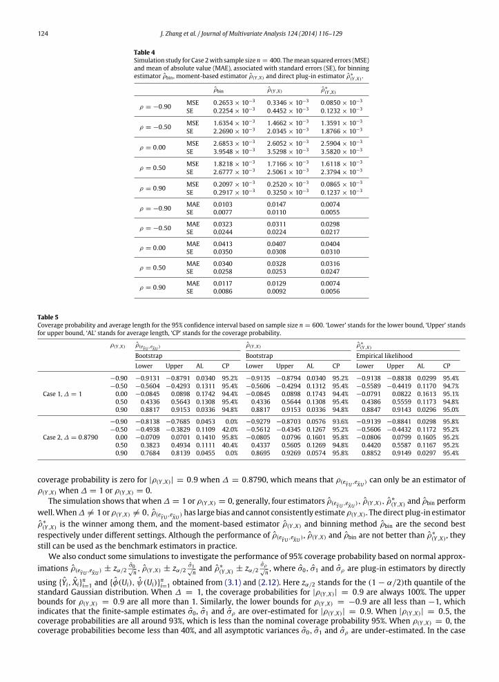
Table 4Simulation study for Case 2with sample size n = 400. Themean squared errors (MSE)and mean of absolute value (MAE), associated with standard errors (SE), for binningestimator ρbin , moment-based estimator ρ(Y ,X) and direct plug-in estimator ρ∗

(Y ,X) .

ρbin ρ(Y ,X) ρ∗

(Y ,X)

ρ = −0.90 MSE 0.2653 × 10−3 0.3346 × 10−3 0.0850 × 10−3

SE 0.2254 × 10−3 0.4452 × 10−3 0.1232 × 10−3

ρ = −0.50 MSE 1.6354 × 10−3 1.4662 × 10−3 1.3591 × 10−3

SE 2.2690 × 10−3 2.0345 × 10−3 1.8766 × 10−3

ρ = 0.00 MSE 2.6853 × 10−3 2.6052 × 10−3 2.5904 × 10−3

SE 3.9548 × 10−3 3.5298 × 10−3 3.5820 × 10−3

ρ = 0.50 MSE 1.8218 × 10−3 1.7166 × 10−3 1.6118 × 10−3

SE 2.6777 × 10−3 2.5061 × 10−3 2.3794 × 10−3

ρ = 0.90 MSE 0.2097 × 10−3 0.2520 × 10−3 0.0865 × 10−3

SE 0.2917 × 10−3 0.3250 × 10−3 0.1237 × 10−3

ρ = −0.90 MAE 0.0103 0.0147 0.0074SE 0.0077 0.0110 0.0055

ρ = −0.50 MAE 0.0323 0.0311 0.0298SE 0.0244 0.0224 0.0217

ρ = 0.00 MAE 0.0413 0.0407 0.0404SE 0.0350 0.0308 0.0310

ρ = 0.50 MAE 0.0340 0.0328 0.0316SE 0.0258 0.0253 0.0247

ρ = 0.90 MAE 0.0117 0.0129 0.0074SE 0.0086 0.0092 0.0056

Table 5Coverage probability and average length for the 95% confidence interval based on sample size n = 600. ‘Lower’ stands for the lower bound, ‘Upper’ standsfor upper bound, ‘AL’ stands for average length, ‘CP’ stands for the coverage probability.

ρ(Y ,X) ρ(eYU ,eXU )ρ(Y ,X) ρ∗

(Y ,X)

Bootstrap Bootstrap Empirical likelihoodLower Upper AL CP Lower Upper AL CP Lower Upper AL CP

Case 1,∆ = 1

−0.90 −0.9131 −0.8791 0.0340 95.2% −0.9135 −0.8794 0.0340 95.2% −0.9138 −0.8838 0.0299 95.4%−0.50 −0.5604 −0.4293 0.1311 95.4% −0.5606 −0.4294 0.1312 95.4% −0.5589 −0.4419 0.1170 94.7%0.00 −0.0845 0.0898 0.1742 94.4% −0.0845 0.0898 0.1743 94.4% −0.0791 0.0822 0.1613 95.1%0.50 0.4336 0.5643 0.1308 95.4% 0.4336 0.5644 0.1308 95.4% 0.4386 0.5559 0.1173 94.8%0.90 0.8817 0.9153 0.0336 94.8% 0.8817 0.9153 0.0336 94.8% 0.8847 0.9143 0.0296 95.0%

Case 2,∆ = 0.8790

−0.90 −0.8138 −0.7685 0.0453 0.0% −0.9279 −0.8703 0.0576 93.6% −0.9139 −0.8841 0.0298 95.8%−0.50 −0.4938 −0.3829 0.1109 42.0% −0.5612 −0.4345 0.1267 95.2% −0.5606 −0.4432 0.1172 95.2%0.00 −0.0709 0.0701 0.1410 95.8% −0.0805 0.0796 0.1601 95.8% −0.0806 0.0799 0.1605 95.2%0.50 0.3823 0.4934 0.1111 40.4% 0.4337 0.5605 0.1269 94.8% 0.4420 0.5587 0.1167 95.2%0.90 0.7684 0.8139 0.0455 0.0% 0.8695 0.9269 0.0574 95.8% 0.8852 0.9149 0.0297 95.4%

coverage probability is zero for |ρ(Y ,X)| = 0.9 when ∆ = 0.8790, which means that ρ(eYU ,eXU ) can only be an estimator ofρ(Y ,X) when∆ = 1 or ρ(Y ,X) = 0.

The simulation shows that when∆ = 1 or ρ(Y ,X) = 0, generally, four estimators ρ(eYU ,eXU ), ρ(Y ,X), ρ∗

(Y ,X) and ρbin performwell.When∆ = 1 orρ(Y ,X) = 0, ρ(eYU ,eXU ) has large bias and cannot consistently estimateρ(Y ,X). The direct plug-in estimatorρ∗

(Y ,X) is the winner among them, and the moment-based estimator ρ(Y ,X) and binning method ρbin are the second bestrespectively under different settings. Although the performance of ρ(eYU ,eXU ), ρ(Y ,X) and ρbin are not better than ρ∗

(Y ,X), theystill can be used as the benchmark estimators in practice.

We also conduct some simulations to investigate the performance of 95% coverage probability based on normal approx-imations ρ(eYU ,eXU ) ± zα/2

σ0√n , ρ(Y ,X) ± zα/2

σ1√n and ρ∗

(Y ,X) ± zα/2σρ√n , where σ0, σ1 and σρ are plug-in estimators by directly

using {Yi, Xi}ni=1 and {φ(Ui), ψ(Ui)}

ni=1 obtained from (3.1) and (2.12). Here zα/2 stands for the (1 − α/2)th quantile of the

standard Gaussian distribution. When ∆ = 1, the coverage probabilities for |ρ(Y ,X)| = 0.9 are always 100%. The upperbounds for ρ(Y ,X) = 0.9 are all more than 1. Similarly, the lower bounds for ρ(Y ,X) = −0.9 are all less than −1, whichindicates that the finite-sample estimates σ0, σ1 and σρ are over-estimated for |ρ(Y ,X)| = 0.9. When |ρ(Y ,X)| = 0.5, thecoverage probabilities are all around 93%, which is less than the nominal coverage probability 95%. When ρ(Y ,X) = 0, thecoverage probabilities become less than 40%, and all asymptotic variances σ0, σ1 and σρ are under-estimated. In the case

J. Zhang et al. / Journal of Multivariate Analysis 124 (2014) 116–129 125

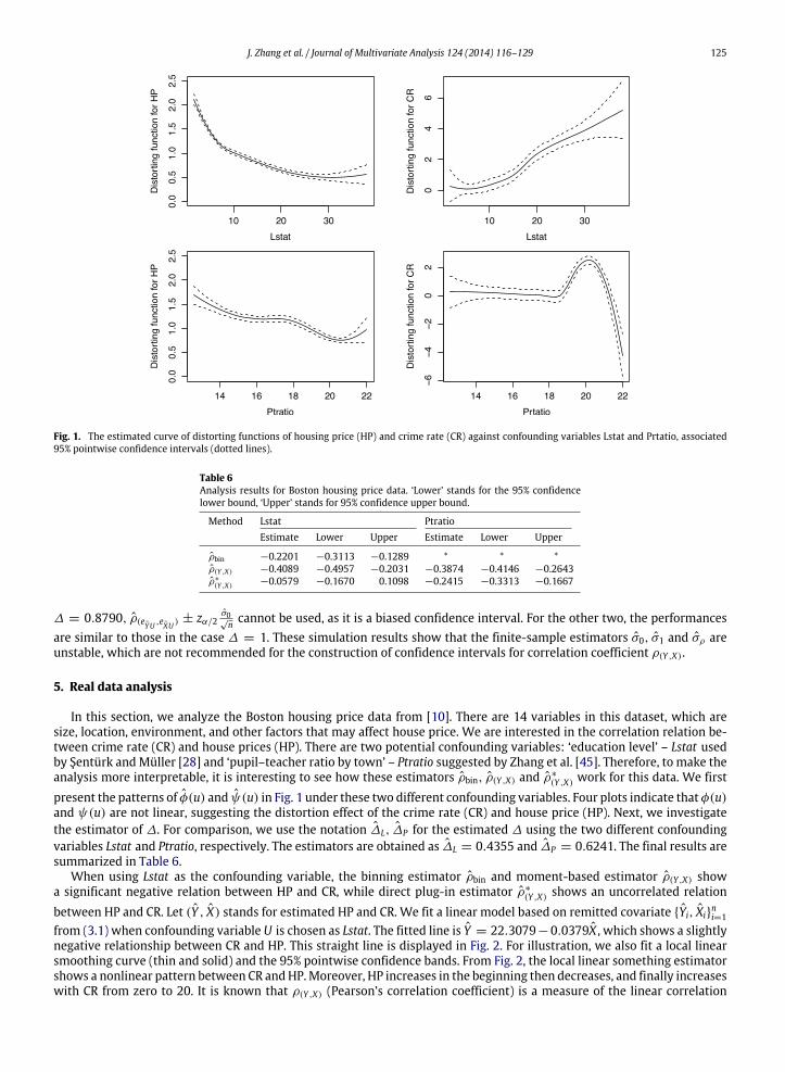
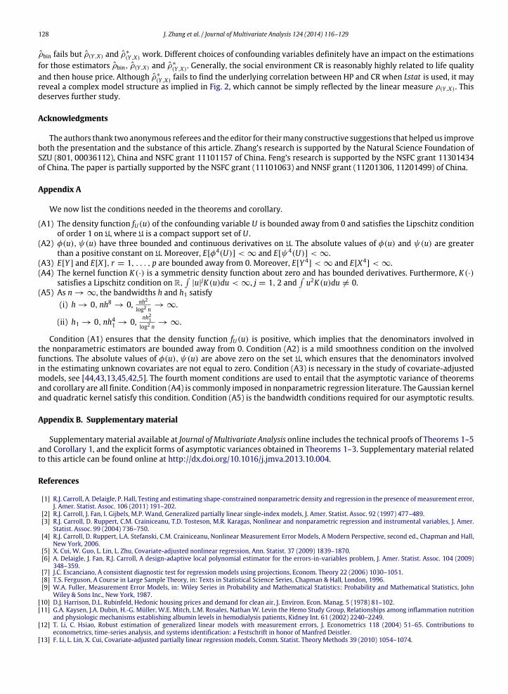
Fig. 1. The estimated curve of distorting functions of housing price (HP) and crime rate (CR) against confounding variables Lstat and Prtatio, associated95% pointwise confidence intervals (dotted lines).

Table 6Analysis results for Boston housing price data. ‘Lower’ stands for the 95% confidencelower bound, ‘Upper’ stands for 95% confidence upper bound.

Method Lstat PtratioEstimate Lower Upper Estimate Lower Upper

ρbin −0.2201 −0.3113 −0.1289 * * *ρ(Y ,X) −0.4089 −0.4957 −0.2031 −0.3874 −0.4146 −0.2643ρ∗

(Y ,X) −0.0579 −0.1670 0.1098 −0.2415 −0.3313 −0.1667

∆ = 0.8790, ρ(eYU ,eXU ) ± zα/2σ0√n cannot be used, as it is a biased confidence interval. For the other two, the performances

are similar to those in the case ∆ = 1. These simulation results show that the finite-sample estimators σ0, σ1 and σρ areunstable, which are not recommended for the construction of confidence intervals for correlation coefficient ρ(Y ,X).

5. Real data analysis

In this section, we analyze the Boston housing price data from [10]. There are 14 variables in this dataset, which aresize, location, environment, and other factors that may affect house price. We are interested in the correlation relation be-tween crime rate (CR) and house prices (HP). There are two potential confounding variables: ‘education level’ – Lstat usedby Şentürk andMüller [28] and ‘pupil–teacher ratio by town’ – Ptratio suggested by Zhang et al. [45]. Therefore, to make theanalysis more interpretable, it is interesting to see how these estimators ρbin, ρ(Y ,X) and ρ∗

(Y ,X) work for this data. We firstpresent the patterns of φ(u) and ψ(u) in Fig. 1 under these two different confounding variables. Four plots indicate thatφ(u)and ψ(u) are not linear, suggesting the distortion effect of the crime rate (CR) and house price (HP). Next, we investigatethe estimator of ∆. For comparison, we use the notation ∆L, ∆P for the estimated ∆ using the two different confoundingvariables Lstat and Ptratio, respectively. The estimators are obtained as ∆L = 0.4355 and ∆P = 0.6241. The final results aresummarized in Table 6.

When using Lstat as the confounding variable, the binning estimator ρbin and moment-based estimator ρ(Y ,X) showa significant negative relation between HP and CR, while direct plug-in estimator ρ∗

(Y ,X) shows an uncorrelated relationbetween HP and CR. Let (Y , X) stands for estimated HP and CR. We fit a linear model based on remitted covariate {Yi, Xi}

ni=1

from (3.1) when confounding variable U is chosen as Lstat. The fitted line is Y = 22.3079−0.0379X , which shows a slightlynegative relationship between CR and HP. This straight line is displayed in Fig. 2. For illustration, we also fit a local linearsmoothing curve (thin and solid) and the 95% pointwise confidence bands. From Fig. 2, the local linear something estimatorshows a nonlinear pattern between CR andHP.Moreover, HP increases in the beginning then decreases, and finally increaseswith CR from zero to 20. It is known that ρ(Y ,X) (Pearson’s correlation coefficient) is a measure of the linear correlation

126 J. Zhang et al. / Journal of Multivariate Analysis 124 (2014) 116–129

Fig. 2. Confounding variable—Lstat. The estimated local smoothing curve of estimated crime rate X (CR) against estimated housing price Y (HP) and theassociated 95% pointwise confidence intervals (dotted lines), and a fitted line Y = 22.3079 − 0.0379X (the straight line).

Fig. 3. Confounding variable—Prtatio. The estimated local smoothing curve of estimated crime rate X (CR) against estimated housing price Y (HP) and theassociated 95% pointwise confidence intervals (dotted lines), and a fitted line Y = 22.3079 − 0.0379X (the straight line).

(dependence) between the two variables Y and X . The nonlinear pattern in Fig. 2 implies that the linear measure ρ∗

(Y ,X) maynot be appropriate. The 95% confidence interval of ρ∗

(Y ,X) in Table 6 implies that there is no linear correlation between HPand CR, but there may exist a nonlinear correlation as indicated in Fig. 2. That is the reason why the direct plug-in estimatorρ∗

(Y ,X) draws a different conclusion from the moment-based estimator ρ(Y ,X).Note that the moment-based estimator ρ(Y ,X) is derived by the correlation coefficient estimator ρ(eYU ,eXU ). It is also inter-

esting to check whether or not the linear correlation measurement ρ(eYU ,eXU ) is appropriate for the choice of confoundingvariable Lstat. We fit a local linear smoothing curve (thin and solid) based on {eiYU , eiXU}

ni=1, associated with the 95% point-

wise confidence band in Fig. 4. The fitted linear regression of eYU = −0.4303 − 0.1220eXU is also presented in this figure.The local linear smoothing in Fig. 4 implies that the relationship between unobservable eYU , eXU is nonlinear, first decreasingand then increasing around zero, but a downward trend in general. This indicates that ρ(eYU ,eXU ) is a reasonable estimatorfor investigating correlation coefficient of (eYU , eXU) to a certain extent.

When using Ptratio as the confounding variable, both moment-based estimator ρ(Y ,X) and direct plug-in estimator ρ∗

(Y ,X)

draw the same conclusion that HP and CR are significant. In Fig. 3, a linear model Y = 23.4062 − 0.3614X shows a strongnegative relationship between CR and HP. Moreover, a local linear smoothing regression shows that HP and CR also have a

J. Zhang et al. / Journal of Multivariate Analysis 124 (2014) 116–129 127

Fig. 4. Confounding variable—Lstat. The estimated local smoothing curve of estimated crime rate residuals eXU (CR-Residuals) against estimated housingprice residuals eYU (HP-Residuals) and the associated 95% pointwise confidence intervals (dotted lines), and a fitted line eYU = −0.4303− 0.1220eXU (thestraight line).

Fig. 5. Confounding variable—Prtatio. The estimated local smoothing curve of estimated crime rate residuals eXU (CR-Residuals) against estimated housingprice residuals eYU (HP-Residuals) and the associated 95% pointwise confidence intervals (dotted lines), and a fitted line eYU = −0.0011− 0.2484eXU (thestraight line).

downward trend. These two observations show that the negative value of ρ∗

(Y ,X) is proper. Next, we check whether the esti-mator ρ(eYU ,eXU ) is appropriate or not. Again, using {eiYU , eiXU }

ni=1, a local linear smoothing curve of eYU against eXU associated

with its 95%pointwise confidence band is fitted andpresented in Fig. 5. A fitted linear regression eYU = −0.0011−0.2484eXUis also presented. Both the linear regression and the local linear smoothing estimator imply that the relationship betweenunobservable eYU , eXU is monotonic non-increasing, which indicates that the negative value of ρ(eYU ,eXU ) is also appropriate,and so is ρ(Y ,X).

For binning estimator ρbin, the choice of confounding variable Ptratio leads to the unreasonable estimator that |ρbin| > 1when the binning number is from 2 to 40. This may be because the binning estimator is a weighted-average of the estimatedvarying coefficient functions and the binning estimation is a less sophisticated nonparametric estimation. Generally, |ρbin| ≤

1 can be guaranteed, however, if the varying coefficient functions are not well estimated by binning estimation, the binningestimator ρbin fails to draw a meaningful conclusion, as indicated in this analysis.

We aim to investigate the underlying correlation between HP and CR in this example. Under the circumstances, whenthe confounding variable is chosen as Lstat, ρbin works [28] but ρ(Y ,X) and ρ∗

(Y ,X) fail as indicated above; If Prtatio is used,

128 J. Zhang et al. / Journal of Multivariate Analysis 124 (2014) 116–129

ρbin fails but ρ(Y ,X) and ρ∗

(Y ,X) work. Different choices of confounding variables definitely have an impact on the estimationsfor those estimators ρbin, ρ(Y ,X) and ρ∗

(Y ,X). Generally, the social environment CR is reasonably highly related to life qualityand then house price. Although ρ∗

(Y ,X) fails to find the underlying correlation between HP and CR when Lstat is used, it mayreveal a complex model structure as implied in Fig. 2, which cannot be simply reflected by the linear measure ρ(Y ,X). Thisdeserves further study.

Acknowledgments

The authors thank two anonymous referees and the editor for theirmany constructive suggestions that helpedus improveboth the presentation and the substance of this article. Zhang’s research is supported by the Natural Science Foundation ofSZU (801, 00036112), China and NSFC grant 11101157 of China. Feng’s research is supported by the NSFC grant 11301434of China. The paper is partially supported by the NSFC grant (11101063) and NNSF grant (11201306, 11201499) of China.

Appendix A

We now list the conditions needed in the theorems and corollary.

(A1) The density function fU(u) of the confounding variable U is bounded away from 0 and satisfies the Lipschitz conditionof order 1 on U, where U is a compact support set of U .

(A2) φ(u), ψ(u) have three bounded and continuous derivatives on U. The absolute values of φ(u) and ψ(u) are greaterthan a positive constant on U. Moreover, E[φ4(U)] < ∞ and E[ψ4(U)] < ∞.

(A3) E[Y ] and E[X], r = 1, . . . , p are bounded away from 0. Moreover, E[Y 4] < ∞ and E[X4

] < ∞.(A4) The kernel function K(·) is a symmetric density function about zero and has bounded derivatives. Furthermore, K(·)

satisfies a Lipschitz condition on R,

|u|jK(u)du < ∞, j = 1, 2 andu2K(u)du = 0.

(A5) As n → ∞, the bandwidths h and h1 satisfy(i) h → 0, nh8

→ 0, nh2

log2 n→ ∞.

(ii) h1 → 0, nh41 → 0, nh21

log2 n→ ∞.

Condition (A1) ensures that the density function fU(u) is positive, which implies that the denominators involved inthe nonparametric estimators are bounded away from 0. Condition (A2) is a mild smoothness condition on the involvedfunctions. The absolute values of φ(u), ψ(u) are above zero on the set U, which ensures that the denominators involvedin the estimating unknown covariates are not equal to zero. Condition (A3) is necessary in the study of covariate-adjustedmodels, see [44,43,13,45,42,5]. The fourth moment conditions are used to entail that the asymptotic variance of theoremsand corollary are all finite. Condition (A4) is commonly imposed in nonparametric regression literature. The Gaussian kerneland quadratic kernel satisfy this condition. Condition (A5) is the bandwidth conditions required for our asymptotic results.

Appendix B. Supplementary material

Supplementarymaterial available at Journal of Multivariate Analysis online includes the technical proofs of Theorems 1–5and Corollary 1, and the explicit forms of asymptotic variances obtained in Theorems 1–3. Supplementary material relatedto this article can be found online at http://dx.doi.org/10.1016/j.jmva.2013.10.004.

References

[1] R.J. Carroll, A. Delaigle, P. Hall, Testing and estimating shape-constrained nonparametric density and regression in the presence ofmeasurement error,J. Amer. Statist. Assoc. 106 (2011) 191–202.

[2] R.J. Carroll, J. Fan, I. Gijbels, M.P. Wand, Generalized partially linear single-index models, J. Amer. Statist. Assoc. 92 (1997) 477–489.[3] R.J. Carroll, D. Ruppert, C.M. Crainiceanu, T.D. Tosteson, M.R. Karagas, Nonlinear and nonparametric regression and instrumental variables, J. Amer.

Statist. Assoc. 99 (2004) 736–750.[4] R.J. Carroll, D. Ruppert, L.A. Stefanski, C.M. Crainiceanu, Nonlinear Measurement Error Models, A Modern Perspective, second ed., Chapman and Hall,

New York, 2006.[5] X. Cui, W. Guo, L. Lin, L. Zhu, Covariate-adjusted nonlinear regression, Ann. Statist. 37 (2009) 1839–1870.[6] A. Delaigle, J. Fan, R.J. Carroll, A design-adaptive local polynomial estimator for the errors-in-variables problem, J. Amer. Statist. Assoc. 104 (2009)

348–359.[7] J.C. Escanciano, A consistent diagnostic test for regression models using projections, Econom. Theory 22 (2006) 1030–1051.[8] T.S. Ferguson, A Course in Large Sample Theory, in: Texts in Statistical Science Series, Chapman & Hall, London, 1996.[9] W.A. Fuller, Measurement Error Models, in: Wiley Series in Probability and Mathematical Statistics: Probability and Mathematical Statistics, John

Wiley & Sons Inc., New York, 1987.[10] D.J. Harrison, D.L. Rubinfeld, Hedonic housing prices and demand for clean air, J. Environ. Econ. Manag. 5 (1978) 81–102.[11] G.A. Kaysen, J.A. Dubin, H.-G. Müller, W.E. Mitch, L.M. Rosales, Nathan W. Levin the Hemo Study Group, Relationships among inflammation nutrition

and physiologic mechanisms establishing albumin levels in hemodialysis patients, Kidney Int. 61 (2002) 2240–2249.[12] T. Li, C. Hsiao, Robust estimation of generalized linear models with measurement errors, J. Econometrics 118 (2004) 51–65. Contributions to

econometrics, time-series analysis, and systems identification: a Festschrift in honor of Manfred Deistler.[13] F. Li, L. Lin, X. Cui, Covariate-adjusted partially linear regression models, Comm. Statist. Theory Methods 39 (2010) 1054–1074.

J. Zhang et al. / Journal of Multivariate Analysis 124 (2014) 116–129 129

[14] G. Li, L. Lin, L. Zhu, Empirical likelihood for a varying coefficient partially linear model with diverging number of parameters, J. Multivariate Anal. 105(2012) 85–111.

[15] H. Lian, Empirical likelihood confidence intervals for nonparametric functional data analysis, J. Statist. Plann. Inference 142 (2012) 1669–1677.[16] H. Liang, W. Härdle, R.J. Carroll, Estimation in a semiparametric partially linear errors-in-variables model, Ann. Statist. 27 (1999) 1519–1535.[17] H. Liang, R. Li, Variable selection for partially linear models with measurement errors, J. Amer. Statist. Assoc. 104 (2009) 234–248.[18] H. Liang, Y. Qin, X. Zhang, D. Ruppert, Empirical likelihood-based inferences for generalized partially linear models, Scandinavian J. Statist. 36 (2009)

433–443.[19] H. Liang, H. Ren, Generalized partially linear measurement error models, J. Comput. Graph. Statist. 14 (2005) 237–250.[20] H. Liang, N. Wang, Partially linear single-index measurement error models, Statist. Sinica 15 (2005) 99–116.[21] D.V. Nguyen, D. Şentürk, Multicovariate-adjusted regression models, J. Stat. Comput. Simul. 78 (2008) 813–827.[22] D.V. Nguyen, D. Şentürk, R.J. Carroll, Covariate-adjusted linear mixed effects model with an application to longitudinal data, J. Nonparametr. Stat. 20

(2008) 459–481.[23] A.B. Owen, Empirical Likelihood, Chapman and Hall/CRC, London, 2001.[24] J. Qin, J. Lawless, Empirical likelihood and general estimating equations, Ann. Statist. 22 (1994) 300–325.[25] D.W. Schafer, Semiparametric maximum likelihood for measurement error model regression, Biometrics 57 (2001) 53–61.[26] S.M. Schennach, Estimation of nonlinear models with measurement error, Econometrica 72 (2004) 33–75.[27] S.M. Schennach, Instrumental variable estimation of nonlinear errors-in-variables models, Econometrica 75 (2007) 201–239.[28] D. Şentürk, H.-G. Müller, Covariate adjusted correlation analysis via varying coefficient models, Scandinavian J. Statist. 32 (2005) 365–383.[29] D. Şentürk, H.-G. Müller, Covariate-adjusted regression, Biometrika 92 (2005) 75–89.[30] D. Şentürk, H.-G. Müller, Inference for covariate adjusted regression via varying coefficient models, Ann. Statist. 34 (2006) 654–679.[31] D. Şentürk, H.-G. Müller, Covariate-adjusted generalized linear models, Biometrika 96 (2009) 357–370.[32] B.W. Silverman, Density Estimation for Statistics and Data Analysis, in: Monographs on Statistics and Applied Probability, Chapman & Hall, London,

1986.[33] W. Stute, W. González Manteiga, M. Presedo Quindimil, Bootstrap approximations in model checks for regression, J. Amer. Statist. Assoc. 93 (1998)

141–149.[34] N. Tang, P. Zhao, Empirical likelihood-based inference in nonlinear regression models with missing responses at random, Statistics 47 (6) (2012)

1141–1159. http://dx.doi.org/10.1080/02331888.2012.658807.[35] N. Tang, P. Zhao, Empirical likelihood semiparametric nonlinear regression analysis for longitudinal data with responsesmissing at random, Ann. Inst.

Statist. Math. 65 (4) (2013) 639–665. http://dx.doi.org/10.1007/s10463-012-0387-4.[36] M.-L. Taupin, Semi-parametric estimation in the nonlinear structural errors-in-variables model, Ann. Statist. 29 (2001) 66–93.[37] L. Wang, C. Hsiao, Method of moments estimation and identifiability of semiparametric nonlinear errors-in-variables models, J. Econometrics 165

(2011) 30–44.[38] X. Wang, G. Li, L. Lin, Empirical likelihood inference for semi-parametric varying-coefficient partially linear EV models, Metrika 73 (2011) 171–185.[39] Z. Wei, L. Zhu, Evaluation of value at risk: an empirical likelihood approach, Statist. Sinica 20 (2010) 455–468.[40] C.-F.J. Wu, Jackknife, bootstrap and other resampling methods in regression analysis, Ann. Statist. 14 (1986) 1261–1350.[41] J. Zhang, S. Feng, G. Li, H. Lian, Empirical likelihood inference for partially linear panel datamodelswith fixed effects, Econom. Lett. 113 (2011) 165–167.[42] J. Zhang, Y. Gai, P. Wu, Estimation in linear regression models with measurement errors subject to single-indexed distortion, Comput. Statist. Data

Anal. 59 (2013) 103–120.[43] J. Zhang, Y. Yu, L. Zhu, H. Liang, Partial linear single index models with distortion measurement errors, Ann. Inst. Statist. Math. 65 (2) (2013) 237–267.

http://dx.doi.org/10.1007/s10463-012-0371-z.[44] J. Zhang, L. Zhu, H. Liang, Nonlinear models with measurement errors subject to single-indexed distortion, J. Multivariate Anal. 112 (2012) 1–23.[45] J. Zhang, L. Zhu, L. Zhu, On a dimension reduction regression with covariate adjustment, J. Multivariate Anal. 104 (2012) 39–55.[46] Y. Zhou, H. Liang, Statistical inference for semiparametric varying-coefficient partially linear models with error-prone linear covariates, Ann. Statist.

37 (2009) 427–458.[47] L. Zhu, L. Lin, X. Cui, G. Li, Bias-corrected empirical likelihood in a multi-link semiparametric model, J. Multivariate Anal. 101 (2010) 850–868.