a review of representation issues and modeling challenges

8/7/2019 A Review of Representation Issues and Modeling Challenges

http://slidepdf.com/reader/full/a-review-of-representation-issues-and-modeling-challenges 1/15

Review

A review of representation issues and modeling challengeswith influence diagrams

Concha Bielza a, Manuel Gomez b, Prakash P. Shenoy c,Ã

a Departamento de Inteligencia Artificial, Universidad Politecnica de Madrid, Boadilla del Monte, Madrid 28660, Spainb Department of Computer Science and Artificial Intelligence, University of Granada, Granada 18071, Spainc School of Business, University of Kansas, Lawrence, KS 66045, USA

a r t i c l e i n f o

Article history:Received 26 October 2009

Accepted 14 July 2010

Processed by B. LevAvailable online 22 July 2010

Keywords:

Decision-making under uncertainty

Influence diagrams

Probabilistic graphical models

Sequential decision diagrams

Unconstrained influence diagrams

Sequential valuation networks

Sequential influence diagrams

Partial influence diagrams

Limited memory influence diagrams

Gaussian influence diagrams

Mixture of Gaussians influence diagrams

Mixture of truncated exponentialsinfluence diagrams

Mixture of polynomials influence diagrams

a b s t r a c t

Since their introduction in the mid 1970s, influence diagrams have become a de facto standard forrepresenting Bayesian decision problems. The need to represent complex problems has led to

extensions of the influence diagram methodology designed to increase the ability to represent complex

problems. In this paper, we review the representation issues and modeling challenges associated with

influence diagrams. In particular, we look at the representation of asymmetric decision problems

including conditional distribution trees, sequential decision diagrams, and sequential valuation

networks. We also examine the issue of representing the sequence of decision and chance variables,

and how it is done in unconstrained influence diagrams, sequential valuation networks, and sequential

influence diagrams. We also discuss the use of continuous chance and decision variables, including

continuous conditionally deterministic variables. Finally, we discuss some of the modeling challenges

faced in representing decision problems in practice and some software that is currently available.

& 2010 Elsevier Ltd. All rights reserved.

Contents

1. Introduction. . . . . . . . . . . . . . . . . . . . . . . . . . . . . . . . . . . . . . . . . . . . . . . . . . . . . . . . . . . . . . . . . . . . . . . . . . . . . . . . . . . . . . . . . . . . . . . . . . . . . . 227

2. Asymmetric decision problems. . . . . . . . . . . . . . . . . . . . . . . . . . . . . . . . . . . . . . . . . . . . . . . . . . . . . . . . . . . . . . . . . . . . . . . . . . . . . . . . . . . . . . . 229

3. Sequencing of decisions and chance variables . . . . . . . . . . . . . . . . . . . . . . . . . . . . . . . . . . . . . . . . . . . . . . . . . . . . . . . . . . . . . . . . . . . . . . . . . . . 232

4. Continuous chance and decision variables. . . . . . . . . . . . . . . . . . . . . . . . . . . . . . . . . . . . . . . . . . . . . . . . . . . . . . . . . . . . . . . . . . . . . . . . . . . . . . 235

5. Modeling with IDs: strengths and limitations . . . . . . . . . . . . . . . . . . . . . . . . . . . . . . . . . . . . . . . . . . . . . . . . . . . . . . . . . . . . . . . . . . . . . . . . . . . 237

6. Summary and discussion. . . . . . . . . . . . . . . . . . . . . . . . . . . . . . . . . . . . . . . . . . . . . . . . . . . . . . . . . . . . . . . . . . . . . . . . . . . . . . . . . . . . . . . . . . . . 238

Acknowledgments . . . . . . . . . . . . . . . . . . . . . . . . . . . . . . . . . . . . . . . . . . . . . . . . . . . . . . . . . . . . . . . . . . . . . . . . . . . . . . . . . . . . . . . . . . . . . . . . . 239

References . . . . . . . . . . . . . . . . . . . . . . . . . . . . . . . . . . . . . . . . . . . . . . . . . . . . . . . . . . . . . . . . . . . . . . . . . . . . . . . . . . . . . . . . . . . . . . . . . . . . . . . 239

1. Introduction

Influence diagrams (IDs) are graphical models for representing

and solving complex decision-making problems based on

uncertain information. Nowadays, they have become a popular

and standard modeling tool. As pointed out in a recent special

issue of the Decision Analysis journal devoted to IDs, these models

‘‘command a unique position in the history of graphical models’’

[62]. They were first used in 1973 by the Decision Analysis Group

at Stanford Research Institute for a project for the Defense

Intelligence Agency. IDs were used to model political conflicts in

the Persian Gulf to see whether more intelligence resources

should be allocated, and they tried to measure the value of

Contents lists available at ScienceDirect

journal homepage: www.elsevier.com/locate/omega

Omega

0305-0483/$- see front matter& 2010 Elsevier Ltd. All rights reserved.

doi:10.1016/j.omega.2010.07.003

Ã Corresponding author. Tel.: +1 785864 7551; fax: +1 785864 5328.

E-mail addresses: [email protected] (C. Bielza), [email protected]

(M. Gomez), [email protected] (P.P. Shenoy).

Omega 39 (2011) 227–241

http://www.elsevier.com/ome

http://dx.doi.org/10.1016/j.omega.2010.07.003

mailto:[email protected]













http://www.elsevier.com/ome



information produced by the Agency. Miller invented the new

graphical convention that we now call an ID. Howard coined the

term ‘‘influence diagram’’. The first resulting (classified) paper on

IDs is [58]. This information is chronicled by the authors of the

facts in [37]. But it is Howard and Matheson’s paper, [34],

reprinted in [36], that is considered to contain the invention of IDs

and to be the pioneering paper. Other interesting details of the

evolution and application of IDs since their inception may be

found in a retrospective article [35].IDs are directed acyclic graphs that may be seen as Bayesian

networks augmented with decision and value nodes. There are

three types of nodes: (1) decision nodes (rectangular) represent-

ing decisions to be made; (2) chance nodes (oval or elliptical)

representing random variables described by probability distribu-

tions; and (3) value nodes (diamond-shaped) representing the

(expected) utilities that model the decision-maker’s preferences

for outcomes. The arcs have different meanings depending

on which node they are directed to: the arcs to chance nodes

indicate probabilistic dependence, the arcs to value nodes indicate

functional dependence, and the arcs to a decision node indicate

what information is known at the time the decision has to be

made. Accordingly, the arcs are called conditional, functional, andinformational, respectively.

At the qualitative (or graphical) level, the ID has a requirement

that there must be a directed path comprising all decision nodes.

It ensures that the ID defines a temporal sequence (total order) of

decisions and it is called the sequencing constraint . As a

consequence, IDs have the ‘‘no-forgetting ’’ property: the decision

maker remembers the past observations and decisions. In

contrast, the transitive closure of the precedence binary relation

induced by the informational arcs is a partial order on the set of

all decision and chance nodes. Therefore, the information

constraints represented by these arcs may not specify a complete

order. From a semantic viewpoint, it means that the decision-

maker may not impose constraints regarding which of two or

more chance nodes must precede the others in the decision-

making process. For example, after deciding to admit a patient

into a hospital, it will not matter which chance variable, ‘‘cost of stay’’ or ‘‘risks of being admitted’’ (infections, contagions, etc.) is

the first to occur.

At the quantitative level, an ID specifies the state spaces of all

decision and chance nodes: a set of alternatives for each decision

variable, and the set of possible values O X of each chance variable

X . Also, a conditional probability table is attached to each chance

node consisting of conditional probability distributions, one for

each state of its parents (direct predecessors), and a real-valued

function, the utility function, is defined over the states of a value

node’s parents. Probabilities and utilities represent beliefs and

preferences, respectively, of the decision maker. When a problem

has a utility function that factorizes additively, each of the

additive factors is represented as a value node.

Fig. 1 shows an example of the graphical part of an ID. Theproblem deals with the oil wildcatter’s problem [69]. An oil

wildcatter has to decide whether to drill or not at a particular site.

He does not know whether the site has oil or not. Before he drills,

he has the option of conducting a seismic test which will reveal

the seismic structure of the site, which is related to oil volume.T and D are decision variables, O and S are chance variables,

and u1 and u2 are value nodes. u1 is a function of the states of T , u2

is a function of the states of D and O. The joint utility function is

the pointwise sum of u1 and u2. As in a Bayesian network, the arcs

directed to chance nodes such as S mean that the conditional

probability attached to S is a function of the states of O and T .

Finally, the informational arcs directed to D say that at the time

the drill decision is made, we know the outcome of S and the

decision made at T . Since we have a directed path (T , S , D), the arc

(T , D) is implied by the no-forgetting condition and could be

omitted. The information constraints specify the (complete) order

given by T , S , D, and O.

IDs were initially proposed as a front-end for decision trees, in

the sense that their compact representation facilitated the

problem structuring, but they were later converted into a decision

tree during the solution process. Although there are now several

efficient algorithms for solving influence diagrams, many still

continue to convert IDs to decision trees during the solution

process (see, e.g., [9]). Olmsted [59] describes a method, that

involves arc reversals, to solve IDs directly without converting

them into decision trees. Shachter [74] published the first ID

evaluation algorithm. Evaluating an ID means computing an

optimal strategy, one that has the maximum expected utility.

Instead of using arc reversals, as in Olmsted’s and Shachter’s

algorithms, other algorithms based on variable elimination

strategies or on clique-trees approaches may now be used to

solve IDs [18,78,38,77,90,52]. Although far from negligible,

computational issues related to ID evaluation are beyond the

scope of this paper. Some critical difficulties and their solutions

are discussed and exemplified in [27,2], where a large ID, calledIctNeo, models neonatal jaundice management for an important

public hospital in Madrid.This paper focuses on modeling issues. IDs have an enormous

potential as a model of uncertain knowledge. The process of

building an ID provides a deep understanding of the problem, and

ID outputs are remarkably valuable. Given a specific configuration

of variables, an ID yields the best course of action. But ID responses

are not limited to provide optimal strategies of the decision-

making problem. Inferred posterior distributions may be employed

to generate diagnosis outputs (probabilities of each cause). IDs

may also automatically generate explanations of their proposals as

a way to justify their reasoning [24,1]. Moreover, the domain

expert may formulate a difficult query, without specifying all the

variables required by the ID to determine the optimal decision. It

will lead to imprecise responses. If we want the decision maker to

receive a convincing response, a refinement is needed, as in [23].By reasoning in the reverse direction, assuming that the final

results of the decisions are known, IDs can be used to generate probabilistic profiles that fit these final results. For example, after a

complete remission of a cancer, endoscopically verified by a

surgery decision, we can be interested in the probability

distributions of other variables, such as patient survival five years

following treatment, side effects, etc. Also, the computation of the

expected value of information has been shown to play a vital role in

assessing the different sources of uncertainty [75].

The aforementioned special issue of Decision Analysis devoted

to IDs is a sign of the lively interest in IDs. Boutilier [6] discusses

the profound impact that IDs have had on artificial intelligence. As

a professional decision analyst, Buede [7] reports on the value of

IDs for tackling challenging real decision problems and considers

Fig. 1. An influence diagram for the oil wildcatter’s problem.

C. Bielza et al. / Omega 39 (2011) 227–241228



IDs almost as indispensable as a laptop computer. Pearl [62]

recognizes the significant relevance of IDs, but he underscores

some limitations. First, due to their initial conception with

emphasis on subjective assessment of parameters, econometri-

cians and social scientists continue to use the traditional path

diagrams, where the parameters are inferred from the data itself.

Second, artificial intelligence researchers, with little interaction

with decision analytic researchers (in the early 1980s), estab-

lished conditional independence semantics using the d-separationcriterion, and developed their own computational tools. Thus,

although IDs are informal precursors to Bayesian networks, the

former had a milder influence on automated reasoning research

than the latter. Finally, Pauker and Wong [61] show that IDs have

disseminated slowly in the medical literature [60,55], compared

to the dominating model of decision trees.

This paper provides a review of ID modeling, discussing the

recent contributions. It aims at bringing closer the theoretical and

practical developments of IDs to foster their wide use. Also, the

analysis identifies challenges and provides insights into the

community involved in the design of decision models using IDs.

The paper is organized as follows. Section 2 discusses the

representation of asymmetric decision problems. Section 3 discusses

the sequencing of decisions and observations that, when partially

specified (or unspecified), leads to another kind of asymmetry.

Section 4 discusses the use of continuous chance and decision

variables, including the use of continuous conditionally determinis-

tic variables. Section 5 discusses some challenges of representing

decision problems in practice. Finally, Section 6 concludes with a

summary, discussion, and an outline of issues not discussed in this

paper.

2. Asymmetric decision problems

In this section, we will define asymmetric decision problems

and review various techniques that have been proposed in

representing such problems based on influence diagrams.

In a decision tree representation, a path from the root node to aleaf node is called a scenario. A decision problem is said to be

symmetric if (i) in all its decision tree representations, the number

of scenarios is equal to the cardinality of the Cartesian product of

the state spaces of all chance and decision variables, and (ii) there

exists a decision tree representation of the problem such that the

sequence of variables is the same in all scenarios. A decision

problem is said to be asymmetric if it is not symmetric.

We will illustrate an asymmetric problem using the reactor

problem, which was originally described by [19], and subse-

quently modified by [4]. An electric utility firm has to decide

whether to build (D2) a reactor of advanced design (a), conven-

tional design (c ), or no reactor (n). If the reactor is successful, i.e.,

there are no accidents, an advanced reactor is more profitable, but

it is riskier. Experience indicates that a conventional reactor (C )has probability 0.98 of being successful (cs) and 0.02 of being a

failure (cf ). On the other hand, an advanced reactor ( A) has

probability 0.66 of being successful (as), probability 0.244 of a

limited accident (al), and probability 0.096 of a major accident

(am). If the firm builds a conventional reactor, the profits are

estimated to be $8B if it is a success, and À$4B if it is a failure. If

the firm builds an advanced reactor, the profits are $12B if it is a

success, À$6B if there is a limited accident, and À$10B if there is

a major accident. The firm’s utility function is linear in dollars.

Before making a decision to build, the firm has an option to

conduct a test (D1 ¼ t ) or not (nt ) of the components of the

advanced reactor at a cost of $1B. The test results (R) can be

classified as bad (b), good ( g ), or excellent (e). Fig. 2 shows a causal

probability model for A and R. Notice that in the probability

model, if A¼ as, then R cannot assume the state b. Thus, if the test

results are observed to be bad, then an advanced reactor will

result in either a limited or major accident (as per the probability

model), and consequently, the Nuclear Regulatory Commission

will not license an advanced reactor.

Fig. 3 shows a decision tree representation of the reactor

problem. The computation of the marginal for R, and the

conditional for A given R, have been done using the causal

probability model for A and R, and this computation is shown inFig. 4. In this figure, the leaves of the tree contain the joint

probabilities for A and R. The optimal strategy is to do the test;

build a conventional reactor if the test results are bad or good, and

build an advanced reactor if the test results are excellent. The

expected profit associated with this strategy is $8.130B.

The decision tree representation, shown in Fig. 3, easily

captures the asymmetric structure of the reactor problem. The

cardinality of the Cartesian product of the state spaces of all

variables is 108, but there are only 21 possible scenarios. The

decision tree is shown using coalescence, i.e., repeating subtrees

are shown only once.

There may be three kinds of asymmetry in asymmetric

decision problems: chance, decision, and information. The state

space of a chance variable may depend on the scenario, and in theextreme, a chance variable may be non-existent. For example, in

the reactor problem, C does not occur in scenarios that includeD2¼a. This is called chance asymmetry. Similarly, the state space

of a decision variable may depend on a scenario, and in the

extreme, may be non-existent. For example, the alternative D2¼ a

is not available in some scenarios. This is called decision

asymmetry. Finally, the sequence of variables may depend on

the scenario. For example, R does not precede D2 in all scenarios.

This is called information asymmetry.

Since decision trees depict all possible scenarios, they can

capture asymmetry easily. However, the number of nodes in a

decision tree grows combinatorially with the number of variables,

and are not tractable for large problems. Also, pre-processing of

probabilities may be required (as in the reactor problem).

as, 0.660

al, 0.244

am, 0.096

g, 0.182

e, 0.818

b, 0.288

g, 0.565

e, 0.147

b, 0.313

g, 0.437

e, 0.250

R

R A

R

Fig. 2. A probability model for A and R in the reactor problem.

C. Bielza et al. / Omega 39 (2011) 227–241 229



Influence diagrams were proposed by Howard and Matheson

[34] to avoid the problem of pre-processing in decision trees and

to represent large problems that would be otherwise intractable

al, 0.060

nt, 0

t, −1

a

n

c

n

c n

a

a

c n

c

12

−6

−10

8

−4

0

12

−6

−10

12

−6

−1010.043

0.649

7.760

5.496

7.760

7.760

7.760

10.043

8.130

b, 0.100

e, 0.600

as, 0.660

al, 0.244

cf, 0.020

as, 0.400

al, 0.460

am, 0.140

as, 0.900

am, 0.040

9.130

g, 0.300

am, 0.096

cs, 0.980

A

AD2

D2

D2

D2

R

D1

C

A

Fig. 3. A decision tree representation and solution of the reactor problem.

0.070

0.138

0.036

0.120

0.540

0.030

0.042

0.024

al, 0.244

g, 0.182

e, 0.818

b, 0.288

g, 0.565

e, 0.147

b, 0.313

g, 0.437

e, 0.250

am, 0.096

as, 0.660 b, 0.100

g, 0.300

e, 0.600

al, 0.700

am, 0.300

as, 0.400

al, 0.460

am, 0.140

as, 0.900

al, 0.060

am, 0.040

0.070

0.030

0.120

0.138

0.042

0.540

0.036

0.024

R

R

R

A R A

A

A

Fig. 4. The pre-processing of probabilities in the reactor problem.

υ2 υ3υ1

A

D1 R' D2

C

Fig. 5. A symmetric ID representation of the reactor problem.

Table 1

The conditional probability distribution for Ru given D1 and A.

P ðRujD1 , AÞ (nt , as) (nt , al) (nt , am) (t , as) (t , al) (t , am)

b 0 0 0 0 0.288 0.313

g 0 0 0 0.182 0.565 0.437

e 0 0 0 0.818 0.147 0.250

nr 1 1 1 0 0 0




using decision trees. However, IDs cannot capture asymmetric

features of decision problems as easily as decision trees. One

solution is to artificially enlarge the state spaces of chance and

decision variables and embed the asymmetric problem in a higher

dimensional symmetric problem. For example, an influence

diagram representation of the reactor problem is shown in Fig. 5.

Variable R in the decision tree has been replaced by Ru which has

state space {b, g , e, nr }, and its conditional distribution now

depends also on D1 as shown in Table 1. Thus, if D1¼nt , then Ru

¼ nr with probability 1, and if D1¼t , then we have the conditional

probability distribution as before. Arc ðRu,D2Þ means the true value

of Ru is known when an alternative of D2 has to be chosen. u1, u2 and

u3 are additive factors of the joint utility function. The constraint

that the alternative D2 ¼ a is not available when Ru ¼ b is modeled

by making Ru a parent of u2 and making the value of u2ðb,a,asÞ ¼

u2ðb,a,alÞ ¼ u2ðb,a,amÞ ¼ ÀM , where M is a large positive number.

This will ensure that when Ru ¼ b, D2¼a will never be optimal, and

the constraint will be satisfied.

This completes a symmetric influence diagram representation

of the reactor problem. Notice that we have increased the size of

the problem in the sense that if we convert the influence diagram

into a decision tree, it would result in 144 scenarios, whereas the

asymmetric decision tree (shown in Fig. 3) only has 21 scenarios.

Thus, the symmetric influence diagram representation is not

very efficient.

To address the inefficiency of the symmetric ID technique,

Smith et al. [85] propose representing the asymmetric aspects of a

decision problem in the conditional distributions, leaving the

overall ID graphical representation unchanged. The conditional

distributions are represented using graphical structures calledconditional distribution trees consisting of conditioning scenarios

and atomic distributions. For example, in the reactor problem, the

conditional distribution trees for D2 and Ru are shown in Fig. 6.

One advantage of conditioning trees is that the number of

scenarios is trimmed back to the minimum necessary. Also,

constraints on decision variables can be represented directly without

having to add large negative utilities. Thus, we do not need to include

an arc from Ru to u2 in the ID graph. However, some disadvantagesremain, such as the artificial state nr for Ru, having D1 as a parent of Ru,

an arc (D1, D2) needs to be added to the ID graph, etc. Bielza and

Shenoy [4] discuss other strengths, weaknesses and open issues

associated with the conditional distribution tree technique.

Next, we will discuss another approach to representing

asymmetric decision problems called sequential decision diagrams

proposed by Covaliu and Oliver [19]. Unlike the conditioning tree

technique, sequential decision diagrams (SDDs) represent the

asymmetric structure of the decision problem directly in the SDD

graph. The SDD graph for the reactor problem is shown in Fig. 7.

Like in IDs, each variable appears once in a SDD. The arcs in a

SDD denote the sequencing of variables in scenarios like in

decision trees. Arcs may be annotated by conditions andconstraints. For example, arc (D1, D2) has a condition D1¼nt ,

which means that whenever D1¼nt , the next variable in the

scenario is D2. If there are any constraints on decisions, then this

can also be listed on the corresponding arc. For example, D2¼a is

only possible if D1¼nt , or if D1¼t and Rab. The details of the

probability model and utility function are not depicted in the SDD

representation. Covaliu and Oliver assume that these details are

represented by a corresponding symmetric influence diagram

(this would be similar to the symmetric ID in Fig. 5, but with only

n

c

n

c

a

g t

e

b

nt nr

nt

t

{ as,

al,

am}

as

al

am

nr, 1 .000

g, 0 .182

e, 0 .818

b, 0 .288

g, 0 .565

e, 0 .147

b, 0 .313

g, 0 .437

e, 0 .250

D1

D1

D2

D2R'

R'

R'

R'

R'

R'

A

A

Fig. 6. The conditional distribution trees for D2 and Ru.

D2 = c

D2 = n

D1 = t

υ

D2 = a|*

D1 = nt

D2D1

A

CR

Fig. 7. A sequential decision diagram for the reactor problem. Ã denotes the

constraint ðD1 ¼ nt Þ3ððD1 ¼ t Þ4ðRabÞÞ.




one value node encoding the joint utility function with all five

variables as parents).

SDDs can represent the set of all scenarios compactly. Also, we

do not need to add dummy states to variables (such as R ¼nr as ID

representations require). On the other hand, there are some

drawbacks. First, SDDs cannot represent probability models

consistently. For example, the ID representation has state space

ORu ¼ fnr ,b, g ,eg for Ru, whereas the SDD representation has

OR ¼ fb,

g ,

eg for R. Second, SDD representation assumes that wehave an unfactored joint utility function. This implies that solving

a SDD cannot be done as efficiently (as we could have if we had an

additive factorization of the joint utility function).

Demirer and Shenoy [20] propose a representation calledsequential valuation networks (SVNs) that is a hybrid of Shenoy’s

[80] asymmetric valuation network and Covaliu and Oliver’s SDDs.

A SVN representation of the reactor problem is shown in Fig. 8.

A SVN consists of an SDD plus indicator, probability and utility

valuations. The SVN has an hexagonal terminal node (instead of

the diamond node in the SDD) whose only role is to signify the

end of a scenario. Solid arcs represent the sequence of variables

in scenarios (as in SDDs). Probability valuations are shown as

single-bordered triangular nodes. The dashed edges connecting

probability valuations to variables denote the domain of the

probability valuation. Thus, the domain of r is { A, R}, the domain

of a is { A}, and the domain of w is {C }. If the probability valuation is

a conditional for a subset of its domain given the rest of the

domain, then the dashed edges to the variables in the subset are

directed towards them. Thus, r is a conditional for {R} given { A}, ais a conditional for { A} given |, and w is a conditional for {C } given

|. The set of all probability valuations denotes a multiplicative

factorization of the joint probability distribution of the chance

nodes in the SVN representation. Indicator valuations encode

qualitative constraints on the joint state spaces of variables and

are represented as double-bordered triangular nodes in the SVN

graph. The reactor problem representation has two indicator

valuations. d1 with domain {R, D2} removes the state (b, a) from

the joint state space of {R, D2}, and d2 with domain {R, A} removes

the state (b, as) from the joint state space of {R, A}. Utilityvaluations represent additive factors of the joint utility function

and are represented by diamond shaped nodes, and the dashed

edges between the utility valuations and variables denote the

domain of the valuations. In practice, many of the values of the

utility factors are zeroes and need not be specified. For example,

the costs associated with building an advanced reactor are only

associated with D2¼a. Thus, this factor is defined on the state

space fag Â O A. This factor is denoted in the SVN representation by

u2ja. Similarly, u3jc with domain {D2, C }, and u4jn with domain {D2}

are utility valuations defined on fc g Â OC and {n}, respectively.

Besides the representations already discussed, there are a

number of other graphical representations proposed in the

literature for asymmetric decision problems. These include

combination of symmetric influence diagrams and decision trees

[8], decision graphs [68], contingent IDs ([25]), asymmetric

valuation networks [80], asymmetric influence diagrams [57],

unconstrained influence diagrams [40], coarse valuation networks[51], and sequential influence diagrams [39].

In spite of the plethora of different graphical representations,

some aspects of asymmetric decision problems are difficult to

represent. One example is a certain event that is repeated a

random number of times. Thus, e.g., we can often find medical

situations where a specific treatment cannot be performed more

than, e.g., twice per full treatment of a patient due to its risks.

Also, that risky treatment must be followed and preceded by a

certain control treatment, etc. Traditional IDs could not meet

these constraints, containing sequences of treatments that are

impossible. For another example, a physician has to decide on a

subset of possible tests and on a sequence for these tests until a

satisfactory diagnosis can be made. If the set of possible tests is

large, the combinatorial explosion of the sequencing of all subsets

makes the problem intractable for representation and solution.

We will discuss this problem in more detail in the next section.

In summary, IDs provide a compact graphical method for

representing and solving symmetric decision problems. For

asymmetric decision problems, several alternative representa-

tions have been proposed, including conditional distribution

trees, sequential decision diagrams, and sequential valuation

networks. While there have been some studies (e.g., [4]) that

compare some of the representations, more studies are needed to

compare all of the different proposed representations.

3. Sequencing of decisions and chance variables

In this section, we will discuss information constraints thatspecify the decisions and chance variables that are observed at the

time a decision has to be made. It also includes a relaxation of the

total order of decisions—sequencing constraint—and those

between decisions and chance variables.

In a symmetric decision problem, the information constraints

are the same in all scenarios. Thus, in the symmetric ID

representation of the reactor problem shown in Fig. 5, for decisionD1 (whether to do a test of the advanced reactor or not), all chance

and decision variables are unobserved, and for decision D2 (type

of reactor to build), the results of the test Ru and decision D1 are

observed, but the true states of C and A are not. This is represented

in the symmetric ID shown in Fig. 5 as follows. Since all chance

and decision variables are unobserved for D1, there are no arrows

into D1. Since the results of test Ru are observed for D2, we haveðRu,D2Þ. Since we have a directed path from D1 to D2, and we are

assuming the no-forgetting condition, the decision made at D1 is

known when a decision at D2 has to be made. This can be modeled

explicitly by including an arc (D1, D2), or implicitly by not having

the arc, but assuming the no-forgetting condition during the

evaluation process.

In asymmetric decision problems, the information constraints

may not be the same in all scenarios. For example, in the decision

tree representation of the reactor problem (shown in Fig. 3), R is

an information predecessor of D2 in some scenarios (when D1¼t ),

but not in some others (when D1¼nt ). While this problem can be

made symmetric as described in the previous section, the

technique described there—adding artificial states to some

chance variables—

cannot be applied in all problems. This is

1 2

D1 = t

D1 = nt

D2 = c

D2 = a

υ1 υ4|n υ2|a υ3|c

D2 = nD1

R

D2

A

T

C

Fig. 8. A sequential valuation network for the reactor problem.




especially true if the chance variable being modified is a parent of

other chance variables since if we add an artificial state to such a

variable, then we have to make up conditional distributions for

each of the child variables that are consistent with the original

joint distribution, which is a non-trivial task.

Consider a problem of diagnosing diabetes. Diabetes can be

detected by doing a blood test and measuring the level of Glucose,

which is elevated for diabetic patients. A less expensive test is to

take a urine specimen and measure the level of Glucose in urine. Aphysician is trying to decide whether or not to treat a patient for

diabetes. Before she makes this decision, she can order a test

(blood or urine). Based on the results of the first test, she can then

decide whether or not to order a second test. A symmetric ID

model for this problem is shown in Fig. 9.

In this model, D is the chance variable diabetes with states d

(has diabetes) and nd (no diabetes), BG is the chance variable

blood Glucose with states bge (elevated) and bgn (normal), GU is

the chance variable Glucose in urine with states gue (elevated)

and gun (normal), FT is the decision variable first test with statesbt (blood test), ut (urine test), and nt (no test), FTR is the chance

variable first test results with states bge, bgn, gue, gun, and nr (no

results), ST is the decision variable second test with the same

states as FT , STR is the chance variable second test results with the

same states as FTR, and TD is the decision variable treatment for

diabetes with states td (treat) and ntd (not treat). u1, u2, and u3 are

additive factors of the joint utility function. FTR and STR are

conditionally deterministic variables with conditional distribu-

tions as follows. If FT ¼bt , and BG¼bge, then FTR¼bge with

probability 1, etc. This formulation allows the possibility of

repeating the same test. An advantage of this formulation is that

we leave the original Bayesian network consisting of arcs (D, BG),

and (D, GU ) unchanged with no artificial states added to the

chance variables. A disadvantage of this formulation is that

we add two artificial chance variables FTR and STR with large state

spaces. Thus, if we have a decision problem with, say 20 possible

tests, formulating a symmetric ID in this fashion would be

intractable to solve.

To deal with diagnosis problems with many possible tests andno ordering specified among them, Jensen and Vomlelova [40]

propose a representation called unconstrained influence diagrams

(UIDs). In UIDs, the requirement that there exists a directed path

that includes all decision variables is dropped. The order of tests is

deliberately unspecified so that there is a partial order among the

decision variables. In the solution phase, we need to determine

the tests to be done in some sequence as a function of what is

observed from the results of the tests that are already done. A UID

model for the diabetes diagnosis problem is shown in Fig. 10.

In this model, D, BG, GU , TD are as before. BT is a decision

variable with states bt and nt , and UT is a decision variable with

states ut and nt. BTR (for blood test results) is a chance variable

with states bge, bgn, and nr , and UTR (for urine test results) is a

chance variable with states gue, gun, and nr. BTR and UTR areconditionally deterministic variables such that if BT ¼bt and

BG¼bge, then BTR¼bge with probability 1, etc. If BT ¼nt , thenBTR¼nr with probability 1 (regardless of the state of BG). Similarly

for UTR. Notice that there is only a partial order among the decision

variables. {BT , UT } precede TD. The ordering between BT and UT is

left unspecified. An optimal solution would include a sequencing of

some tests as a function of what is observed from the previous tests

performed. If BT is the first test and UT is the second test, then BTR

becomes an informational predecessor of UT , etc.

An advantage of UIDs is that the state spaces of some of the

decision and chance variables are much smaller than in a

corresponding symmetric ID. For example, the state spaces of BT and UT have cardinality two, whereas in the symmetric

ID representation, FT and ST have cardinality three. Also, thestate spaces of BTR and UTR have cardinality three, whereas

the corresponding variables FTR and STR have cardinality five.

Furthermore, BTR and UTR each have two parents, whereas the

corresponding variables FTR and STR each have three parents. (We

should note here that BTR and UTR have different semantics thanFTR and STR. The latter are artificial variables that are constructed

to represent the information asymmetry inherent in the decision

problem.) These differences in the number of states are even more

accentuated with the number of tests. Thus, if we have a diagnosis

problem with say 10 possible tests, a UID representation may be

tractable for solution even though a symmetric ID is not.

UIDs are designed to simplify the representation of diagnosis/

troubleshooting problems, and they are not appropriate for the

general class of decision problems. Also, the evaluation procedure

υ3

υ2 υ1

ST STR FTR FT TD

GUBG

D

Fig. 9. A symmetric ID model for the diabetes diagnosis problem.

κ 2

υ3

κ 1

TDUTBT

BTR UTR

GUBG

D

Fig. 10. An unconstrained ID model for the diabetes diagnosis problem.




for solving UIDs is much more complex than the procedure for

solving a symmetric ID since the sequencing of the tests is not

specified and has to be determined in the solution phase. When

the number of possible tests is large, solving a UID may also be

intractable. At this stage, there is no study on the size of diagnosis

problems that can be solved using UIDs. As computing power

increases, problems that are intractable today may be tractable in

the future.

In principle, a decision tree representation should be able toeasily represent the asymmetric features of the diabetes diagnosis

problem. A drawback would be the size of the decision tree. Since

sequential valuation networks are able to represent a decision

tree compactly, this representation could be used to represent this

problem using no artificial variables. A SVN representation of the

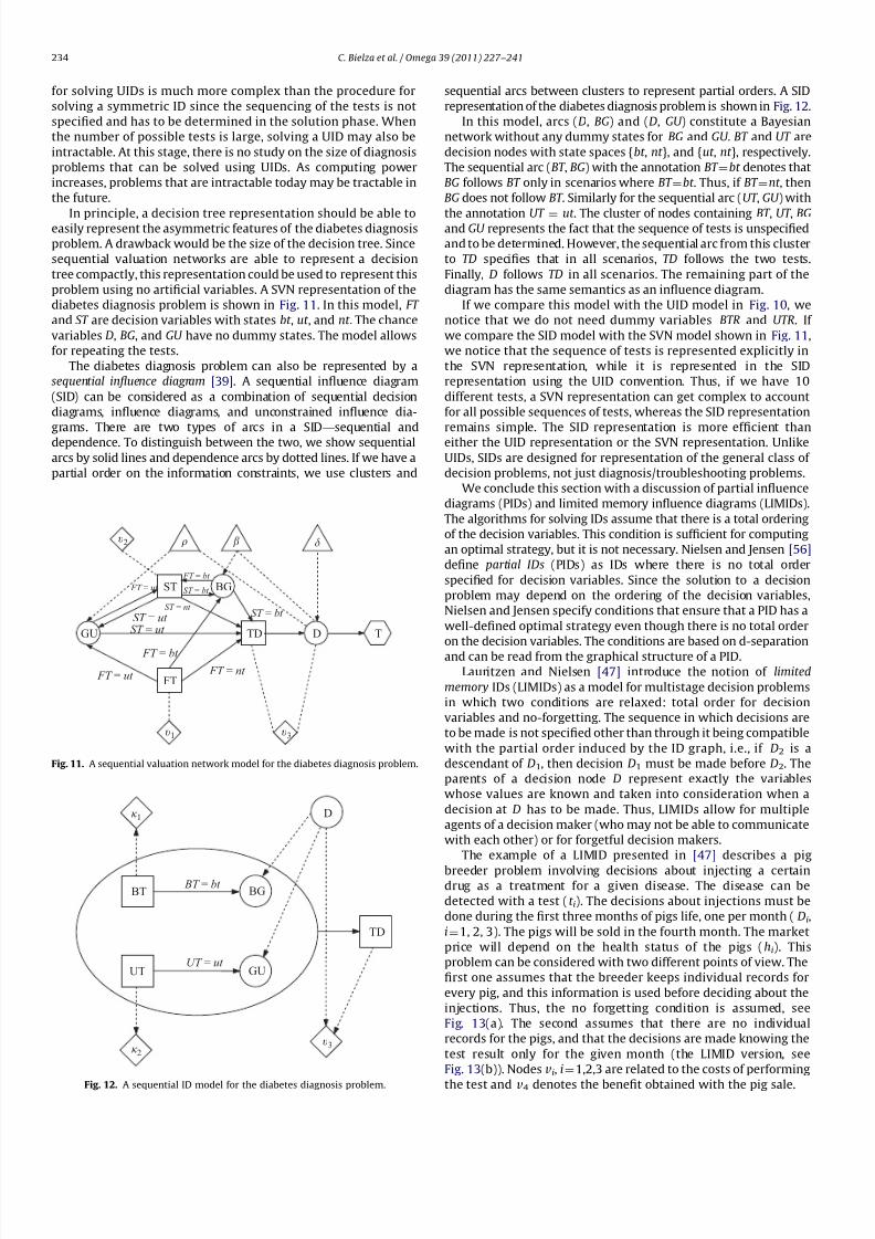
diabetes diagnosis problem is shown in Fig. 11. In this model, FT

and ST are decision variables with states bt , ut , and nt . The chance

variables D, BG, and GU have no dummy states. The model allows

for repeating the tests.

The diabetes diagnosis problem can also be represented by asequential influence diagram [39]. A sequential influence diagram

(SID) can be considered as a combination of sequential decision

diagrams, influence diagrams, and unconstrained influence dia-

grams. There are two types of arcs in a SID—sequential and

dependence. To distinguish between the two, we show sequential

arcs by solid lines and dependence arcs by dotted lines. If we have a

partial order on the information constraints, we use clusters and

sequential arcs between clusters to represent partial orders. A SID

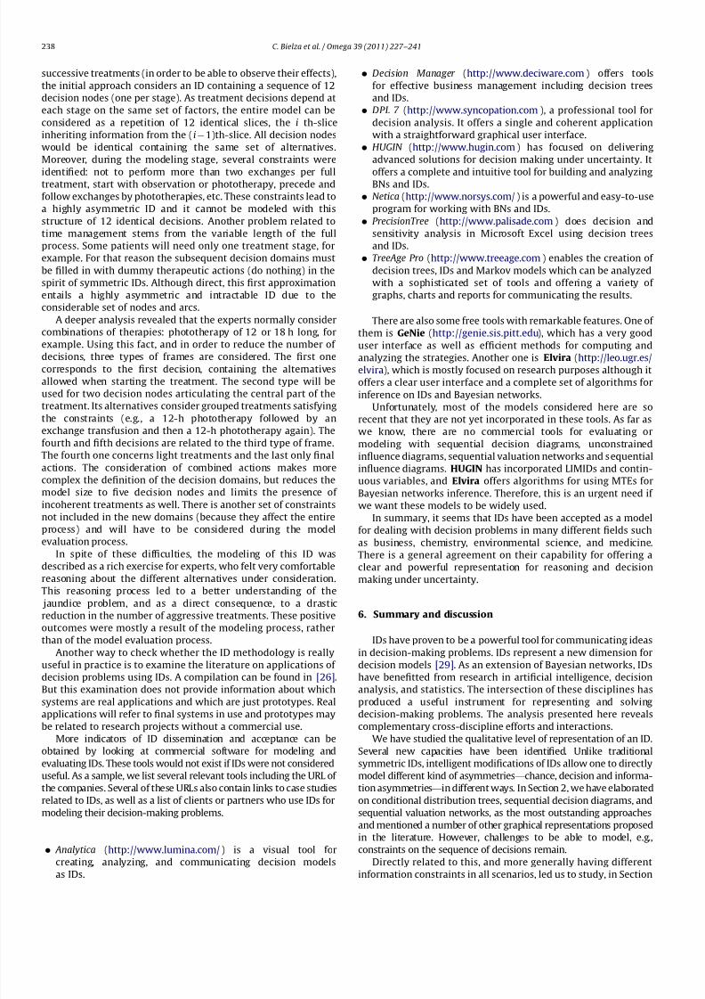
representation of the diabetes diagnosis problem is shown in Fig. 12.

In this model, arcs (D, BG) and (D, GU ) constitute a Bayesian

network without any dummy states for BG and GU. BT and UT are

decision nodes with state spaces {bt , nt }, and {ut , nt }, respectively.

The sequential arc (BT , BG) with the annotation BT ¼ bt denotes thatBG follows BT only in scenarios where BT ¼bt . Thus, if BT ¼nt , thenBG does not follow BT . Similarly for the sequential arc (UT , GU ) with

the annotation UT ¼ ut . The cluster of nodes containing BT , UT , BGand GU represents the fact that the sequence of tests is unspecified

and to be determined. However, the sequential arc from this cluster

to TD specifies that in all scenarios, TD follows the two tests.

Finally, D follows TD in all scenarios. The remaining part of the

diagram has the same semantics as an influence diagram.

If we compare this model with the UID model in Fig. 10, we

notice that we do not need dummy variables BTR and UTR. If

we compare the SID model with the SVN model shown in Fig. 11,

we notice that the sequence of tests is represented explicitly in

the SVN representation, while it is represented in the SID

representation using the UID convention. Thus, if we have 10

different tests, a SVN representation can get complex to account

for all possible sequences of tests, whereas the SID representation

remains simple. The SID representation is more efficient than

either the UID representation or the SVN representation. Unlike

UIDs, SIDs are designed for representation of the general class of

decision problems, not just diagnosis/troubleshooting problems.

We conclude this section with a discussion of partial influence

diagrams (PIDs) and limited memory influence diagrams (LIMIDs).

The algorithms for solving IDs assume that there is a total ordering

of the decision variables. This condition is sufficient for computing

an optimal strategy, but it is not necessary. Nielsen and Jensen [56]

define partial IDs (PIDs) as IDs where there is no total order

specified for decision variables. Since the solution to a decision

problem may depend on the ordering of the decision variables,

Nielsen and Jensen specify conditions that ensure that a PID has a

well-defined optimal strategy even though there is no total order

on the decision variables. The conditions are based on d-separation

and can be read from the graphical structure of a PID.Lauritzen and Nielsen [47] introduce the notion of limited

memory IDs (LIMIDs) as a model for multistage decision problems

in which two conditions are relaxed: total order for decision

variables and no-forgetting. The sequence in which decisions are

to be made is not specified other than through it being compatible

with the partial order induced by the ID graph, i.e., if D2 is a

descendant of D1, then decision D1 must be made before D2. The

parents of a decision node D represent exactly the variables

whose values are known and taken into consideration when a

decision at D has to be made. Thus, LIMIDs allow for multiple

agents of a decision maker (who may not be able to communicate

with each other) or for forgetful decision makers.

The example of a LIMID presented in [47] describes a pig

breeder problem involving decisions about injecting a certaindrug as a treatment for a given disease. The disease can be

detected with a test (t i). The decisions about injections must be

done during the first three months of pigs life, one per month (Di,

i ¼1, 2, 3). The pigs will be sold in the fourth month. The market

price will depend on the health status of the pigs (hi). This

problem can be considered with two different points of view. The

first one assumes that the breeder keeps individual records for

every pig, and this information is used before deciding about the

injections. Thus, the no forgetting condition is assumed, see

Fig. 13(a). The second assumes that there are no individual

records for the pigs, and that the decisions are made knowing the

test result only for the given month (the LIMID version, see

Fig. 13(b)). Nodes vi, i ¼ 1,2,3 are related to the costs of performing

the test and v4 denotes the benefit obtained with the pig sale.

ST = ut ST = nt

ST = bt

FT = nt

FT = bt

FT = ut

ST = ut

FT = bt

ST = bt FT = ut

υ2

υ1 υ3

FT

TD D T

BGST

GU

Fig. 11. A sequential valuation network model for the diabetes diagnosis problem.

UT = ut

BT = bt

κ 1

υ3κ 2

TD

BG

GUUT

BT

D

Fig. 12. A sequential ID model for the diabetes diagnosis problem.




The main motivation of LIMIDs is that by limiting the number

of information arcs, its solution is computationally tractable

whereas the same decision problem could be intractable if we

assumed the no-forgetting condition. The disadvantage is that anoptimal solution of a LIMID may not be optimal for the same

decision problem if we were to assume the no-forgetting

condition. Thus, we trade-off tractability of solution with

optimality. Lauritzen and Nilsson describe an algorithm calledsingle policy updating for finding a local optimal solution of a

LIMID. Thus, if we consider the ID in Fig. 10 as a LIMID, and solve

it using the single policy updating algorithm, assuming that no

test pays by itself, a solution may be that no test shall be done,

even though an optimal UID solution for the problem is to first do

a urine test, and if positive, then do a blood test.

In summary, we have examined different representations

of problems in which we have information asymmetry. We

have examined symmetric influence diagrams, unconstrained

influence diagrams, sequential valuation networks, sequentialinfluence diagrams, partial influence diagrams, and limited

memory influence diagrams. For the class of problems in which

we have several diagnostic tests that can be done in any sequence,

the sequential influence diagram representation is very efficient

in representing such problems. The exact solution of these

problems, however, is hard and may not be tractable when we

have a large number of tests. In some decision problems, there

may not be a total order specified among the decision nodes,

but it admits a well-defined optimal solution through the use of

partial influence diagrams. Also, for a class of multi-stage

problems, influence diagrams may be intractable. By dropping

the no-forgetting condition, the solution of a decision problem

may be tractable using the single policy updating algorithm

of LIMIDs.

4. Continuous chance and decision variables

In this section, we review the literature on the use and issues

related to using continuous chance and decision variables in

representing and solving decision problems.

In practice, it is safe to assume that one encounters chance and

decision variables that are continuous. A chance or decision variable

is said to be discrete if the state space is countable, and continuous

otherwise. Typically, the states of discrete variables are symbols,whereas the states of continuous variables are real numbers. The

conditional distribution of continuous chance variables are typically

conditional probability density functions (PDFs). One major problem

associated with solving IDs with continuous chance variables is

integration of products of conditional PDFs and utility functions

when computing expected utilities. There are many commonly used

PDFs, such as the Gaussian PDF, that cannot be integrated in closed

form. Another major problem is finding the maximum of a utility

function on the state space of a continuous decision variable.

Depending on the nature of the multidimensional utility function,

we can have a difficult non-linear optimization problem. To avoid

these difficulties, one standard approach is to discretize the

continuous variables using bins. Using many bins results in a

computational burden for solving the discrete ID, and using too few

bins leads to an unacceptable approximation of the problem.

One of the earliest work on using continuous variables in IDs is

by Kenley and Shachter [42,76]. In their representation, which

they call Gaussian IDs (GIDs), all chance variables are continuous

having the so-called conditional linear Gaussian (CLG) distribu-

tion. This is a Gaussian PDF, whose mean is a linear function of its

parents, and the variance is a constant. An implication of this

condition is that the joint distribution of all chance variables is

multivariate normal. One can find marginals of the multivariate

normal distribution without doing any integration. So the

problem of integration does not exist for such IDs. GIDs also

assume that all decision nodes are continuous and that the utility

function is a quadratic function of its parent chance and decision

variables. An implication of this condition is that there is a unique

maximum for the decision variables, which can be found in closedform. Thus, the optimization problem of finding an optimal

solution does not exist either for such IDs.

An example of a GID is shown in Fig. 14 [76]. A consultant

has purchased an expensive computer for use in her practice.

She will bill her clients for computer usage at an hourly rate.

Also, she expects to have the computer unused most of the

time and she would like to sell some of these idle hours to time-

sharing users. She must decide on a price for her consulting

clients, and a price for her time-sharing users, so as to maximize

her total profit.

She believes that the number of consulting hours sold will

depend on consulting price, and that the cost of the computer

facilities for consulting, consulting cost, will depend on consulting

hours. Her accountant will work up a consulting estimate of thenumber of consulting hours she will bill. This will be known

before deciding on the price for time-sharing users. The number of

time-share hours will depend on time share price and the hours

the computer is not busy with consulting work (idle hours). The

cost of running the time-sharing service, time sharing cost, will

depend on the hours purchased, time share hours, and idle hours.

Her profit will be the difference between total revenues and costs.

Specific parameters for the Gaussian distributions attached to all

the continuous variables must be assessed. These are shown in

Fig. 14, with the corresponding conditional mean and conditional

variance next to each node. All continuous variables (chance or

decision) are depicted with a double border.

Poland [64] extends GIDs to mixture of Gaussians IDs

(MoGIDs). In MoGIDs, we have discrete and continuous chance

ID version

LIMID version

υ1 υ2 υ3

υ4h1 h2 h3 h4

t3t2t1

D3D2D1

υ1 υ2 υ3

υ4h4h3h2h1

t1 t2

D1

D2

D3

t3

Fig. 13. The ID and limited memory ID model for the pig problem.




variables. As in GIDs, continuous variables have a CLG distribution

whose mean is a linear function of its continuous parents, and a

constant variance. The linear function and constant variance can

be different for each state of its discrete parents. However,

discrete nodes cannot have continuous parents. An implication of

these conditions is that given a state of each discrete variable, the

joint distribution of the continuous variables is multivariate

normal. Again the problem of integration does not exist. MoGIDs

have the same restriction as GIDs regarding utility functions

associated with continuous decision variables (quadratic).

An example of a MoGID is shown in Fig. 15 [64]. This is a

different formulation of the oil wildcatter’s problem than the onegiven earlier in Fig. 1. The previous formulation discretizes oil

volume and drilling cost (included in u2). Here, they are

represented as continuous variables (with double borders). Oil

volume has a mixed distribution: it has a PDF for positive volumes

but there is a probability mass at zero. Poland includes these two

variables conditioned by ‘‘case’’ (discrete) variables to make their

PDF mixtures. For example, oil volume case has three states:

‘‘zero’’, ‘‘medium’’ and ‘‘high’’, with associated probabilities

conditioned on seismic structure. For each of these, oil volume

has a distinct distribution: a probability mass at zero for the

‘‘zero’’ case, and a PDF for the other cases.

If we have a continuous variable whose conditional PDF is not

CLG, then we can approximate it with a mixture of Gaussians. The

parameters of the mixture distribution (number of distributions,

weights, and means and variances of the Gaussian distributions)

can be found either by using a minimum entropy technique [65]

or by solving a non-linear optimization problem that minimizes

some distance measure between the target distribution and

mixture distribution [81].

If we have a discrete chance variable with a continuous parent,

then we do not have a mixture of multivariate normal distribution

for the continuous chance variables. Some authors suggest

approximating the product of the conditionals for the discrete

variable and its parents by a CLG using a variational approach [54]

or a numerical integration called Gaussian quadrature [49]. Shenoy

[81] suggests using arc reversals to remedy this situation. However,arc reversals may destroy the CLG distribution of the parent, in

which case, it has to be approximated by a mixture of Gaussians.

If besides continuous chance variables, we have a decision

problem with (few) continuous decision variables, Bielza et al. [3]

suggest the use of a Markov Chain Monte Carlo (simulation)

method for finding an approximately optimal strategy as a

remedy for the optimization and integration problem. They define

an artificial distribution on the product space of chance and

decision variables, such that sampling from this artificial

augmented probability model is equivalent to solving the original

decision problem. The approach can accommodate arbitrary

probability models and utility functions.

Charnes and Shenoy [10] investigate the problem of solving

large IDs with continuous chance variables and discrete decision

CC |ch ∼

N (58000 + 4ch, 4000000)

CH |cp ∼

N (1500 − 5cp, 40000)

CE |ch ∼

N (1500 + ch, 250000)

TC |(th,ih) ∼

N (5000 + 1.25th − 1.25ih, 40000)

TH |(tp,ih) ∼

N (750 − 10tp + 0.05ih,10000)

P =CP ·CH + TP ·TH

−CC −TC

IH |ch ∼

N (3500 − 3ch, 100)

Time Share

Hours (TH)

Time Share

Cost (TC)

Time Share

Price (TP)

Consulting

Price (CP)

Consulting

Hours (CH)

Consulting

Cost (CC)

Consulting

Estimate (CE)Profit (P)

Idle

Hours (IH)

Fig. 14. A Gaussian ID for the Consultant’s-problem.

Seismic

Structure (S)

Seismic

Test? (T)

Oil

Case (OS)

Oil

Volume (O)

Test

Results (TR)

Profit (P)

Cost

Case (CS)

Drilling

Cost (DC)

Drill?

(D)Utility

Fig. 15. A MoGID for the oil wildcatter’s problem.




variables using a Monte Carlo method where only a small set of

chance variables are sampled for each decision node. Using this

technique, they solve a problem of valuation of a Bermudan put

option with 30 discrete decision variables and continuous chance

variables with non-CLG distributions.

Another strategy for easing the problem of integration is

suggested by Moral et al. [53]. They suggest approximating

conditional PDFs by mixtures of exponential functions whose

exponent is a linear function of the state of the variable and itscontinuous parents. Each mixture component (or piece) is

restricted to a hypercube. One advantage of this approximation

is that such mixtures of truncated exponentials (MTEs) are easy to

integrate in closed form. Also, the family of MTE functions are

closed under multiplication and integration, operations used in

solving influence diagrams. Cobb et al. [17] describe MTE

approximations of commonly used PDFs using an optimization

technique similar to the one described earlier for finding

parameters of a mixture of Gaussian approximation. Cobb and

Shenoy [16] define MTE IDs, where we have continuous chance

variables with MTE conditional PDFs, discrete decision variables,

and utility functions that are also MTE functions. Such MTE IDs

can be solved using the solution technique of discrete IDs with

integration used to marginalize continuous chance variables.

Cobb [13] introduces continuous decision MTE influence diagrams

(CDMTEIDs), where besides using MTE potentials to approximate

PDFs and utility functions, continuous decision variables are

allowed. A piecewise-linear decision rule for these continuous

decision variables is developed.

In the same spirit as MTEs, Shenoy and West [82,84] suggest

the use of mixture of polynomials (MOPs) to approximate

conditional PDFs. Like MTE functions, MOP functions are easy to

integrate, and the family of MOP functions is closed under

multiplication and integration. Unlike MTEs, finding MOP approx-

imations is easier for differentiable functions as one can use the

Taylor series expansion to find a MOP approximation. Finding an

MTE approximation for a multi-dimensional distribution (such as

the conditional for a variable given another continuous variables

as parents) can be difficult, whereas finding a MOP approximationis easier at it can be found using the multi-dimensional version of

the Taylor series.

In an ID, a continuous chance variable is said to be deterministic

if the variances of its conditional distributions (for each state of its

parents) are all zeroes. An example of a deterministic variable is a

continuous variable whose state is a deterministic function of its

continuous parents, and the function may depend on the state of

its discrete parents. An example of a deterministic variable isProfit ¼RevenueÀCost , where Revenue and Cost are continuous

chance variables, and Profit is a deterministic variable withRevenue and Cost as parents. Deterministic variables pose a

special problem since the joint density for all the chance variables

does not exist. For GIDs and MoGIDs, deterministic variables are

not a problem as long as the functions defining the deterministicvariables are linear. The theory of multivariate normal distribu-

tions allows linear deterministic functions [71,46]. The class of

MTE functions is also closed under transformations required by

linear deterministic functions [14], but not for non-linear

deterministic functions. For non-linear deterministic functions,

Cobb and Shenoy [15] suggest approximating a non-linear

deterministic function by a piecewise linear function, and then

using the technique proposed in [14]. Cinicioglu and Shenoy [11]

describe an arc reversal theory for hybrid Bayesian networks

with deterministic variables with a differentiable deterministic

function. They use Dirac delta functions [22] to represent

deterministic functions. The deterministic function does not have

to be linear or even invertible. As long it is differentiable and its

real zeroes can be found, arc reversal can be described in closed

form. They conjecture that Olmsted’s arc-reversal theory [59] for

solving discrete IDs can be used for hybrid IDs using their arc-

reversal theory. This claim needs further investigation. The family

of MOP functions are closed for a larger class of deterministic

functions than MTEs. For example, MOP functions can be used for

quotients [82]. Li and Shenoy [50] describe a further extension of

the extended Shenoy–Shafer architecture [83] for solving influ-

ence diagrams containing discrete, continuous, and deterministic

variables. In problems where no divisions need to be done, MOPapproximations can be used for PDFs, utility functions, and

deterministic functions to alleviate the problems of integration

and optimization. Finally, deterministic variables pose no problems

for Monte Carlo methods, such as [10], that use independent and

identically distributed samples. However, Markov chain Monte

Carlo methods may not converge in the presence of deterministic

variables.

We conclude this section by remarking that much research

remains to be done to make the solution of IDs with continuous

chance and decision variables viable in practice. It would be very

useful to have a formal comparison of the various techniques on a

test bed of problems with different sizes and complexity. This

includes a comparison of MoGIDs, MTE IDs, and MOP IDs. Also, for

an individual technique, such as, e.g., MTE IDs, there are many

ways to approximate a PDF by an MTE function. There is a tradeoff

between number of exponential terms and number of pieces

(mixture components). Fewer pieces invariably imply more

exponential terms. It is not known which approximation is the

best from a computational viewpoint. A similar issue exists for

MoGIDs and MOP IDs. Finally, it would be useful to have bounds

on the optimality of the solution based on bounds on the

approximations of the PDFs.

5. Modeling with IDs: strengths and limitations

The previous sections have presented ID modeling capabilities

and challenges mostly developed and identified by researchers

and published in scientific forums. But there is not much feedbackfrom analysts and experts about their experiences with IDs for

building decision-making models. Specifically, it would be

interesting to know the main problems perceived by those who

have tried to model complex decision-making problems using IDs.

Unfortunately, it is well known that the modeling step is not yet

automated, and is considered as an art, and in which most of the

literature has taken little interest [12]. Perhaps this is the reason

why there are very few papers offering this point of view. Two

examples of these are [2,27].

These papers describe the problems faced while modeling a

neonatal jaundice management problem in the medical domain.

This problem is present during the first few days of a baby’s life,

the first 72 h after birth being the most critical. The first decision

is whether to admit (or not) a baby to a hospital and confining it,eventually, to an intensive care unit. In case the baby is admitted,

it is necessary to control the bilirubin levels, carrying out different

tests, and applying some of the prescribed treatments: photo-

therapy, exchange transfusion, or observation. The treatment will

be selected depending on some crucial factors such as age, weight,

and bilirubin and hemoglobin levels. Treatments are given along

several consecutive stages, observing after each one their effects

on the baby and repeating the process as many times as necessary

until the problem is solved (the infant is then discharged or (s)he

receives a treatment related to another disease).

The two main problems identified when constructing an ID for

this disease are related to time modeling and the existence of

constraints between the treatments (both are closely related).

Since experts consider that there must be at least 6 h between two




successive treatments (in order to be able to observe their effects),

the initial approach considers an ID containing a sequence of 12

decision nodes (one per stage). As treatment decisions depend at

each stage on the same set of factors, the entire model can be

considered as a repetition of 12 identical slices, the i th-slice

inheriting information from the (i À 1)th-slice. All decision nodes

would be identical containing the same set of alternatives.

Moreover, during the modeling stage, several constraints were

identified: not to perform more than two exchanges per fulltreatment, start with observation or phototherapy, precede and

follow exchanges by phototherapies, etc. These constraints lead to

a highly asymmetric ID and it cannot be modeled with this

structure of 12 identical decisions. Another problem related to

time management stems from the variable length of the full

process. Some patients will need only one treatment stage, for

example. For that reason the subsequent decision domains must

be filled in with dummy therapeutic actions (do nothing) in the

spirit of symmetric IDs. Although direct, this first approximation

entails a highly asymmetric and intractable ID due to the

considerable set of nodes and arcs.

A deeper analysis revealed that the experts normally consider

combinations of therapies: phototherapy of 12 or 18 h long, for

example. Using this fact, and in order to reduce the number of

decisions, three types of frames are considered. The first one

corresponds to the first decision, containing the alternatives

allowed when starting the treatment. The second type will be

used for two decision nodes articulating the central part of the

treatment. Its alternatives consider grouped treatments satisfying

the constraints (e.g., a 12-h phototherapy followed by an

exchange transfusion and then a 12-h phototherapy again). The

fourth and fifth decisions are related to the third type of frame.

The fourth one concerns light treatments and the last only final

actions. The consideration of combined actions makes more

complex the definition of the decision domains, but reduces the

model size to five decision nodes and limits the presence of

incoherent treatments as well. There is another set of constraints

not included in the new domains (because they affect the entire

process) and will have to be considered during the modelevaluation process.

In spite of these difficulties, the modeling of this ID was

described as a rich exercise for experts, who felt very comfortable

reasoning about the different alternatives under consideration.

This reasoning process led to a better understanding of the

jaundice problem, and as a direct consequence, to a drastic

reduction in the number of aggressive treatments. These positive

outcomes were mostly a result of the modeling process, rather

than of the model evaluation process.

Another way to check whether the ID methodology is really

useful in practice is to examine the literature on applications of

decision problems using IDs. A compilation can be found in [26].

But this examination does not provide information about which

systems are real applications and which are just prototypes. Realapplications will refer to final systems in use and prototypes may

be related to research projects without a commercial use.

More indicators of ID dissemination and acceptance can be

obtained by looking at commercial software for modeling and

evaluating IDs. These tools would not exist if IDs were not considered

useful. As a sample, we list several relevant tools including the URL of

the companies. Several of these URLs also contain links to case studies

related to IDs, as well as a list of clients or partners who use IDs for

modeling their decision-making problems.

Analytica (http://www.lumina.com/) is a visual tool for

creating, analyzing, and communicating decision models

as IDs.

Decision Manager (http://www.deciware.com) offers tools

for effective business management including decision trees

and IDs.

DPL 7 (http://www.syncopation.com ), a professional tool for

decision analysis. It offers a single and coherent application

with a straightforward graphical user interface.

HUGIN (http://www.hugin.com) has focused on delivering

advanced solutions for decision making under uncertainty. It

offers a complete and intuitive tool for building and analyzingBNs and IDs.

Netica (http://www.norsys.com/) is a powerful and easy-to-use

program for working with BNs and IDs.

PrecisionTree (http://www.palisade.com ) does decision and

sensitivity analysis in Microsoft Excel using decision trees

and IDs.

TreeAge Pro (http://www.treeage.com) enables the creation of

decision trees, IDs and Markov models which can be analyzed

with a sophisticated set of tools and offering a variety of

graphs, charts and reports for communicating the results.

There are also some free tools with remarkable features. One of

them is GeNie (http://genie.sis.pitt.edu), which has a very good

user interface as well as efficient methods for computing andanalyzing the strategies. Another one is Elvira (http://leo.ugr.es/

elvira), which is mostly focused on research purposes although it

offers a clear user interface and a complete set of algorithms for

inference on IDs and Bayesian networks.

Unfortunately, most of the models considered here are so

recent that they are not yet incorporated in these tools. As far as

we know, there are no commercial tools for evaluating or

modeling with sequential decision diagrams, unconstrained

influence diagrams, sequential valuation networks and sequential

influence diagrams. HUGIN has incorporated LIMIDs and contin-

uous variables, and Elvira offers algorithms for using MTEs for

Bayesian networks inference. Therefore, this is an urgent need if

we want these models to be widely used.

In summary, it seems that IDs have been accepted as a model

for dealing with decision problems in many different fields such

as business, chemistry, environmental science, and medicine.

There is a general agreement on their capability for offering a

clear and powerful representation for reasoning and decision

making under uncertainty.

6. Summary and discussion

IDs have proven to be a powerful tool for communicating ideas

in decision-making problems. IDs represent a new dimension for

decision models [29]. As an extension of Bayesian networks, IDs

have benefitted from research in artificial intelligence, decision

analysis, and statistics. The intersection of these disciplines has

produced a useful instrument for representing and solvingdecision-making problems. The analysis presented here reveals

complementary cross-discipline efforts and interactions.

We have studied the qualitative level of representation of an ID.

Several new capacities have been identified. Unlike traditional

symmetric IDs, intelligent modifications of IDs allow one to directly

model different kind of asymmetries—chance, decision and informa-

tion asymmetries—in different ways. In Section 2, we have elaborated

on conditional distribution trees, sequential decision diagrams, and

sequential valuation networks, as the most outstanding approaches

and mentioned a number of other graphical representations proposed

in the literature. However, challenges to be able to model, e.g.,

constraints on the sequence of decisions remain.

Directly related to this, and more generally having different

information constraints in all scenarios, led us to study, in Section


http://www.lumina.com/

http://www.deciware.com/

http://www.syncopation.com/

http://www.hugin.com/

http://www.norsys.com/

http://www.palisade.com/

http://www.treeage.com/

http://genie.sis.pitt.edu/

http://leo.ugr.es/elvira




http://genie.sis.pitt.edu/

http://www.treeage.com/

http://www.palisade.com/

http://www.norsys.com/

http://www.hugin.com/

http://www.syncopation.com/

http://www.deciware.com/

http://www.lumina.com/



3, the contributions made to the so-called sequencing constraint.

Examples include diagnosis/troubleshooting problems. The main

models here are the unconstrained IDs, the sequential valuation

network and the sequential IDs, where the requirement of a

directed path including all decision variables is dropped. Sequen-

tial influence diagram representation is very efficient. However,

when the number of decisions without constraints is large,

solving these models may be intractable. The limited memory

influence diagrams drop the no-forgetting condition, which maymake problems that are intractable to solve exactly tractable for

an approximate solution. The challenge here is, perhaps, to design

‘‘anytime’’ algorithms to find an approximate solution when

having time constraints that prevent completion of an exact

algorithm.

We have discussed some literature and challenges associated

with the use of continuous chance and decision variables in IDs.

This is an area that is ripe for further research on the use of

mixture of truncated exponentials (MTE) functions and mixture of

polynomials (MOP) functions to approximate PDFs and utility

functions. Using the extended Shenoy–Shafer architecture [50],

the MTE and MOP functions can be propagated in a binary join

tree [79] to compute an optimal strategy.

We have not gone into other issues that are also important and

are listed as follows:

Decisions may involve groups of people rather than single

decision makers [66,87,44,21,72].

Beyond the typical what-if questions on the quantitative

values of the ID, perturbations of the ID may also include itsstructure, i.e., critical evaluation of functional relations on

variables is also necessary. This also involves the complicated

and burdensome process of generating an ID. Ideas here range

from suggesting a case-based reasoning approach where

candidate IDs are retrieved from a set of similar IDs (a case

base) [48], to using a neural network for yielding an initial ID

that is later refined to generate a well-formed ID [43].

Explanation capabilities of IDs are a key element that canimprove the effectiveness and justification of decisions. Ex-

planations enhance the decision maker’s ability to understand

and have confidence in the ID model, thereby accepting ID

advices. Generating explanations is related to the search of the

most relevant information and how to present it to the decision

maker in a structured form. Although in Bayesian networks

there has been much research in the topic, see a review in [45],

we expect to see more work in decision-making [41,5,28].

Modeling temporal processes is one of the greatest challenges

of IDs. Dynamic IDs [86], and temporal IDs [67], are possibilities

that have in (partially observable) Markov decision processes a

strong competitor.

The need to deal with time- or modeling-pressured situations

in developing time-critical dynamic decision support systems isa practically useful but difficult problem. Xiang and Poh

[88,89] consider time-critical dynamic IDs to choose, from a

meta-reasoning approach, the best model with optimal trade-

off between model quality and computational tractability.

Other authors construct anytime algorithms providing approx-

imate strategies incrementally refined as computation pro-

gresses [30–33,63,70].

A daunting challenge would be to face the continuous change

in the environment. IDs are difficult to scale up and adapt to

changing and evolving knowledge, policies, standards, regula-

tions, operating procedures, etc. Perhaps IDs were not

conceived to reach so far. However, combining the inclusion

of time together with a mechanism that detects when the ID

fails and suggests an alternative model is a possibility. These

adaptive models have been the topic of many recent world

conferences, like that organized by AAAI in 2005.

Moreover, models need to effectively operate in the rapidly

developing distributed infrastructures, gathering knowledge

from different sources [73], like from different computers in a

network.

Acknowledgments

We are very grateful for discussions with T.D. Nielsen and J.Q.

Smith during the workshop on ‘‘Graphical Modelling of Depen-

dent Uncertainties for Decision Support in Public Policy’’ in

August 2004. Thanks also to T. Bedford who convinced C. Bielza to

prepare a talk in that workshop about challenges in large

decision-making problems that served as the seed of this paper.

Research partially supported by the Spanish Ministry of

Education and Science, Projects TIN2007-62626 and TIN2007-

67418-C03-03.

References

[1] Bielza C, Fernandez del Pozo J, Lucas P. Explaining clinical decisions byextracting regularity patterns. Decision Support Systems 2008;44:397–408.

[2] Bielza C, Gomez M, Rıos-Insua S, Fernandez del Pozo J. Structural, elicitationand computational issues faced when solving complex decision problems withinfluence diagrams. Computers and Operations Research 2000;27(7–8):725–40.

[3] Bielza C, Muller P, Rıos D. Decision analysis by augmented probabilitysimulation. Management Science 1999;45(7):995–1007.

[4] Bielza C, Shenoy PP. A comparison of graphical techniques for asymmetricdecision problems. Management Science 1999;45(11):1552–69.

[5] Bohanec M, Rajkovic V. Knowledge-based explanation in multiattributedecision making. In: Computer aided decision analysis: theory and applica-tions. Westport: Quorum Books; 1993. p. 189–204.

[6] Boutilier C. The influence of influence diagrams on artificial intelligence.Decision Analysis 2005;2(4):229–31.

[7] Buede D. Influence diagrams: a practitioner’s perspective. Decision Analysis2005;2(4):235–7.

[8] Call H, Miller W. A comparison of approaches and implementations forautomating decision analysis. Reliability Engineering and System Safety

1990;30:115–62.[9] Canbolat YB, Chelst K, Garg N. Combining decision tree and MAUT for selecting

a country for a global manufacturing facility. Omega 2007;35(3):312–25.[10] Charnes JM, Shenoy PP. Multi-stage Monte Carlo method for solving influence

diagrams using local computation. Management Science 2004;50(3):405–18.[11] Cinicioglu EN, Shenoy PP. Arc reversals in hybrid Bayesian networks with

deterministic variables. International Journal of Approximate Reasoning2009;50(5):763–77.

[12] Clemen R. Making hard decisions: an introduction to decision analysis.South-Western College Pub.; 1997.

[13] Cobb BR. Influence diagrams with continuous decision variables and non-Gaussian uncertainties. Decision Analysis 2007;4(3):136–55.

[14] Cobb BR, Shenoy PP. Hybrid Bayesian networks with linear deterministicvariables. In: Bacchus F, Jaakkola T, editors. Uncertainty in artificialintelligence: proceedings of the 21st conference. Corvallis, OR: AUAI Press;2005. p. 136–44.

[15] Cobb BR, Shenoy PP. Nonlinear deterministic relationships in Bayesiannetworks. In: Godo L, editor. Symbolic and quantitative approaches to

reasoning with uncertainty: eighth European conference, ECSQARU 2005.Lecture notes in artificial intelligence, vol. 3571. Berlin: Springer; 2005. p.27–38.

[16] Cobb BR, Shenoy PP. Decision making with hybrid influence diagrams usingmixtures of truncated exponentials. European Journal of OperationalResearch 2008;186(1):261–75.

[17] Cobb BR, Shenoy PP, Rumi R. Approximating probability density functions inhybrid Bayesian networks with mixtures of truncated exponentials. Statistics& Computing 2006;16(3):293–308.

[18] Cooper G. A method for using belief networks as influence diagrams. In:Proceedings of the fourth conference on uncertainty in artificial intelligence.Minneapolis: University of Minnesota; 1988. p. 55–63.

[19] Covaliu Z, Oliver R. Representation and solution of decision problems usingsequential decision diagrams. Management Science 1995;41(12):1860–81.

[20] Demirer R, Shenoy PP. Sequential valuation networks for asymmetric decisionproblems. European Journal of Operational Research 2006;169(1):286–309.

[21] Detwarasiti A, Shachter RD. Influence diagrams for team decision analysis.Decision Analysis 2005;2(4):207–28.

[22] Dirac PAM. The physical interpretation of the quantum dynamics. Proceed-

ings of the Royal Society of London, Series A 1927;113(765):621–41.




[23] Fernandez del Pozo J, Bielza C. An interactive framework for open queries indecision support systems. In: Garijo F, Riquelme J, Toro M, editors. Advancesin artificial intelligence—IBERAMIA 2002. Lecture notes in artificial intelli-gence, vol. 2527. Berlin: Springer; 2002. p. 254–64.

[24] Fernandez del Pozo J, Bielza C, Gomez M. A list-based compact representationfor large decision tables management. European Journal of OperationalResearch 2005;160(3):638–62.

[25] Fung RM, Shachter RD. Contingent influence diagrams. Technical Report,Department of Engineering-Economic Systems, Stanford University, Stanford,California; 1990.

[26] Gomez M. Real-world applications of influence diagrams. In: Gamez J, MoralS, Salmeron A, editors. Advances in Bayesian networks. Studies in fuzzinessand soft computing, vol. 146. Berlin: Springer-Verlag; 2004. p. 161–80.

[27] Gomez M, Bielza C, Fernandez del Pozo J, Rıos-Insua S. A graphicaldecision—theoretic model for neonatal jaundice. Medical Decision Making2007;27:250–65.

[28] Gonul M, Onkal D, Lawrence M. The effects of structural characteristics of explanations on use of a DSS. Decision Support Systems 2006;42:1481–93.

[29] Helfand M, Pauker S. Influence diagrams: a new dimension for decisionmodels. Medical Decision Making 1997;17(3):351–2.

[30] Horsch M, Poole D. Flexible policy construction by information refinement.In: Horvitz E, Jensen FV, editors. Uncertainty in artificial intelligence:proceedings of the 12th conference. San Francisco, CA: Morgan Kaufmann;1996. p. 315–24.

[31] Horsch M, Poole D. An anytime algorithm for decision making underuncertainty. In: Cooper G, Moral S, editors. Uncertainty in artificialintelligence: proceedings of the 14th conference. San Francisco: MorganKaufmann; 1998. p. 246–55.

[32] Horsch M, Poole D. Estimating the value of computation in flexible

information refinement. In: Laskey K, Prade H, editors. Uncertainty inartificial intelligence: proceedings of the 15th conference. San Francisco,CA: Morgan Kaufmann; 1999. p. 297–304.

[33] Horvitz E, Seiver A. Time-critical action: representations and application. In:Geiger D, Shenoy PP, editors. Uncertainty in artificial intelligence: proceed-ings of the 13th conference. San Francisco, CA: Morgan Kaufmann; 1997. p.250–7.

[34] Howard R, Matheson J. Influence diagrams. In: Howard R, Matheson J, editors.Readings on the principles and applications of decision analysis, vol. II.Strategic Decisions Group; 1984. p. 719–62.

[35] Howard R, Matheson J. Influence diagram retrospective. Decision Analysis2005;2:144–7.

[36] Howard R, Matheson J. Influence diagrams. Decision Analysis 2005;2:127–43.

[37] Howard R, Matheson J, Merkhofer M, Miller A, North D. Comment oninfluence diagram retrospective. Decision Analysis 2006;3:117–9.

[38] Jensen F, Jensen FV, Dittmer D. From influence diagrams to junction trees. In:de Mantaras R, Poole D, editors. Uncertainty in artificial intelligence:proceedings of the 10th conference. San Francisco, CA: Morgan Kaufmann;

1994. p. 367–73.[39] Jensen FV, Nielsen TD, Shenoy PP. Sequential influence diagrams: a unifiedasymmetry framework. International Journal of Approximate Reasoning2006;42(1–2):101–18.

[40] Jensen FV, Vomlelova M. Unconstrained influence diagrams. In: Darwiche A,Friedman N, editors. Uncertainty in artificial intelligence: proceedings of the18th conference. San Francisco, CA: Morgan Kaufmann; 2002. p. 234–41.

[41] Jimison H, Fagan L, Shachter R, Shortliffe E. Patient-specific explanation inmodels of chronic disease. Artificial Intelligence in Medicine 1992;4:191–205.

[42] Kenley CR. Influence diagram models with continuous variables. PhD thesis,Stanford University, Stanford, CA; 1986.

[43] Kim J, Lee K, Lee J. Hybrid of neural network and decision knowledgeapproach to generating influence diagrams. Expert Systems with Applications2002;23(3):237–44.

[44] Koller D, Milch B. Multi-agent influence diagrams for representing andsolving games. Games and Economic Behavior 2003;45(1):181–221.

[45] Lacave C, Dıez F. A review of explanation methods for heuristic expertsystems. Knowledge Engineering Review 2004;19:133–46.

[46] Lauritzen SL, Jensen FV. Stable local computation with conditional Gaussiandistributions. Statistics and Computing 2001;11:191–203.

[47] Lauritzen SL, Nilsson D. Representing and solving decision problems withlimited information. Management Science 2001;47(9):1235–51.

[48] Lee J, Kim J, Kim S. A methodology for modeling influence diagrams: a case-based reasoning approach. International Journal of Intelligent Systems inAccounting, Finance & Management 2000;9(1):55–63.

[49] Lerner U, Segal E, Koller D. Exact inference in networks with discrete childrenof continuous parents. In: Breese J, Koller D, editors. Uncertainty in artificialintelligence: proceedings of the 17th conference. San Francisco, CA: MorganKaufmann; 2001. p. 319–28.

[50] Li Y, Shenoy PP. Solving hybrid influence diagrams with deterministicvariables. In: Grunwald P, Spirtes P, editors. Uncertainty in artificialintelligence: proceedings of the 26th conference (UAI-2010). Corvallis, OR:AUAI Press; 2010. p. 322–31.

[51] Liu L, Shenoy PP. Representing asymmetric decision problems using coarsevaluations. Decision Support Systems 2004;37(1):119–35.

[52] Madsen AL, Jensen FV. Lazy evaluation of symmetric Bayesian decision

problems. In: Laskey K, Prade H, editors. Uncertainty in artificial intelligence:

proceedings of the 15th conference. San Francisco, CA: Morgan Kaufmann;1999. p. 382–90.

[53] Moral S, Rumı R, Salmeron A. Mixtures of truncated exponentials in hybridBayesian networks. In: Benferhat S, Besnard P, editors. Symbolic andquantitative approaches to reasoning with uncertainty: sixth Europeanconference, ECSQARU-2001. Lecture notes in artificial intelligence, vol. 2143.Berlin: Springer; 2001. p. 156–67.

[54] Murphy K. A variational approximation for Bayesian networks with discreteand continuous latent variables. In: Laskey K, Prade H, editors. Uncertainty inartificial intelligence: proceedings of the 15th conference. San Francisco, CA:Morgan Kaufmann; 1999. p. 457–66.

[55] Nease R, Owens D. Use of influence diagrams to structure medical decisions.Medical Decision Making 1997;17:263–75.

[56] Nielsen TD, Jensen FV. Well defined decision scenarios. In: Laskey KB, PradeH, editors. Uncertainty in artificial intelligence: proceedings of the 15thconference. San Francisco, CA: Morgan Kaufmann; 1999. p. 502–11.

[57] Nielsen TD, Jensen FV. Representing and solving asymmetric decisionproblems. International Journal of Information Technology and DecisionMaking 2003;2(2):217–63.

[58] North D, Miller A, Braunstein T. Decision analysis of intelligence resourceallocation. Technical Report DAH C15-73-C-0430, Stanford Research Institute,Menlo Park, CA; 1974.

[59] Olmsted S. On representing and solving decision problems. PhD thesis,Department of Engineering-Economic Systems, Stanford, CA; 1983.

[60] Owens D, Shachter R, Nease R. Representation and analysis of medical decisionproblems with influence diagrams. Medical Decision Making 1997;17:241–62.

[61] Pauker S, Wong J. The influence of influence diagrams in medicine. DecisionAnalysis 2005;2(4):238–44.

[62] Pearl J. Influence diagrams-historical and personal perspectives. Decision

Analysis 2005;2:232–4.[63] Poh K, Horvitz E. Reasoning about the value of decision-model refinement:

methods and application. In: Heckerman D, Mamdani A, editors. Uncertaintyin artificial intelligence: proceedings of the 11th conference. San Francisco,CA: Morgan Kaufmann; 1993. p. 174–82.

[64] Poland III WB. Decision analysiswith continuous and discrete variables: a mixturedistribution approach. PhD thesis, Stanford University, Stanford, CA; 1994.

[65] Poland III WB, Shachter RD. Mixtures of Gaussians and minimum relativeentropy techniques for modeling continuous uncertainties. In: Heckerman D,Mamdani A, editors. Uncertainty in artificial intelligence: proceedings of theninth conference. San Francisco, CA: Morgan Kaufmann; 1993. p. 183–90.

[66] Poole D. The independent choice logic for modelling multiple agents underuncertainty. Artificial Intelligence 1997;94:7–56.

[67] Provan G, Clarke J. Dynamic network construction and updating techniquesfor the diagnosis of acute abdominal pain. IEEE Transactions on PatternAnalysis and Machine Intelligence 1993;15(3):299–307.

[68] Qi R, Zhang N, Poole D. Solving asymmetric decision problems with influencediagrams. In: de Mantaras R, Poole D, editors. Uncertainty in artificial

intelligence: proceedings of the 10th conference. San Francisco, CA: MorganKaufmann; 1994. p. 491–7.

[69] Raiffa H. Decision analysis. Reading, MA: Addison-Wesley; 1968.

[70] Ramoni M. Anytime influence diagrams. In: Proceedings of the IJCAIworkshop on anytime algorithms and deliberation scheduling. AmericanAssociation for Artificial Intelligence; 1995. p. 55–62.

[71] Rao CR. Linear statistical inference and its applications. In: Wiley series inprobability and mathematical statistics. 2nd ed.. Wiley; 1973.

[72] Rıos J, Rıos-Insua D. Negotiation over influence diagrams. Technical Report,Rey Juan Carlos University; 2006.

[73] Schneeweiss C. Distributed decision making. 2nd ed.. New York: Springer;2003.

[74] Shachter RD. Evaluating influence diagrams. Operations Research 1986;34:871–82.

[75] Shachter RD. Efficient value of information computation. In: Laskey KB, PradeH, editors. Uncertainty in artificial intelligence: proceedings of the 15thconference. San Francisco, CA: Morgan Kaufmann; 1999. p. 594–602.

[76] Shachter RD, Kenley CR. Gaussian influence diagrams. Management Science1989;35(5):527–50.

[77] Shachter RD, Ndilikilikesha PP. Using potential influence diagrams forprobabilistic inference and decision making. In: Heckerman D, Mamdani A,editors. Uncertainty in artificial intelligence: proceedings of the 15thconference. San Francisco, CA: Morgan Kaufmann; 1993. p. 383–90.

[78] Shenoy PP. Valuation-based systems for Bayesian decision analysis. Opera-tions Research 1992;40(3):463–84.

[79] Shenoy PP. Binary join trees for computing marginals in the Shenoy–Shaferarchitecture. International Journal of Approximate Reasoning 1997;17(2–3):239–63.

[80] Shenoy PP. Valuation network representation and solution of asymmetricdecision problems. European Journal of Operational Research 2000;121(3):579–608.

[81] Shenoy PP. Inference in hybrid Bayesian networks using mixtures of Gaussians. In: Dechter R, Richardson T, editors. Uncertainty in artificialintelligence: proceedings of the 22nd conference. Corvallis, OR: AUAI Press;2006. p. 428–36.

[82] Shenoy PP, West JC. Inference in hybrid Bayesian networks using mixtures of polynomials. Working paper 321, University of Kansas School of Business,

Lawrence, KS; May 2009.




[83] Shenoy PP, West JC. Inference in hybrid Bayesian networks with determinis-tic variables. In: Sossai C, Chemello G, editors. Symbolic and quantitativeapproaches to reasoning with uncertainty—10th ECSQARU. Lecture notes inartificial intelligence, vol. 5590. Berlin: Springer-Verlag; 2009. p. 46–58.

[84] Shenoy PP, West JC. Mixtures of polynomials in hybrid Bayesian networkswith deterministic variables. In: Kroupa T, Vejnarova J, editors. Proceedings of the eighth workshop on uncertainty processing, Prague, Czech Republic:University of Economics; 2009. p. 202–12.

[85] Smith J, Holtzman S, Matheson J. Structuring conditional relationships ininfluence diagrams. Operations Research 1993;41(2):280–97.

[86] Tatman JA, Shachter RD. Dynamic programming and influence diagrams. IEEE

Transactions on Systems, Man and Cybernetics 1990;20(2):365–79.

[87] Xiang Y. Probabilistic reasoning in multiagent systems: a graphical modelsapproach. Cambridge University Press; 2002.

[88] Xiang Y, Poh K. Time-critical dynamic decision making. In: Laskey K, Prade H,editors. Uncertainty in artificial intelligence: proceedings of the 15thconference. San Francisco, CA: Morgan Kaufmann; 1999. p. 688–95.

[89] Xiang Y, Poh K. Time-critical dynamic decision modeling in medicine.Computers in Biology and Medicine 2002;32(2):85–97.

[90] Zhang NL. Probabilistic inference in influence diagrams. In: Cooper G, Moral S,editors. Uncertainty in artificial intelligence: proceedings of the 14th

conference. San Francisco, CA: Morgan Kaufmann; 1998. p. 514–22.


a review of representation issues and modeling challenges

Documents