a review and assessment of land-use change models ... · pdf filea review and assessment of...
TRANSCRIPT

United StatesDepartment ofAgriculture
Forest Service
NortheasternResearch Station
General TechnicalReport NE-297
Chetan AgarwalGlen M. GreenJ. Morgan GroveTom P. EvansCharles M. Schweik
A Review and Assessmentof Land-Use Change Models:Dynamics of Space, Time,and Human Choice
Indiana University
Center for theStudy of Institutions,Population, andEnvironmental Change

Abstract
Land-use change models are used by researchers and professionals to explore the dynamicsand drivers of land-use/land-cover change and to inform policies affecting such change. Abroad array of models and modeling methods are available to researchers, and each type hascertain advantages and disadvantages depending on the objective of the research. This reportpresents a review of different types of models as a means of exploring the functionality andability of different approaches. In this review, we try to explicitly incorporate human processes,because of their centrality in land-use/land-cover change. We present a framework tocompare land-use change models in terms of scale (both spatial and temporal) andcomplexity, and how well they incorporate space, time, and human decisionmaking. Initially,we examined a summary set of 250 relevant citations and developed a bibliography of 136papers. From these 136 papers a set of 19 land-use models were reviewed in detail asrepresentative of the broader set of models identified from the more comprehensive review ofliterature. Using a tabular approach, we summarize and discuss the 19 models in terms ofdynamic (temporal) and spatial interactions, as well as human decisionmaking as defined bythe earlier framework. To eliminate the general confusion surrounding the term scale, weevaluate each model with respect to pairs of analogous parameters of spatial, temporal, anddecisionmaking scales: (1) spatial resolution and extent, (2) time step and duration, and (3)decisionmaking agent and domain. Although a wide range of spatial and temporal scales iscovered collectively by the models examined, we find most individual models occupy a muchmore limited spatio-temporal niche. Many raster models we examined mirror the extent andresolution of common remote-sensing data. The broadest-scale models are, in general, notspatially explicit. We also find that models incorporating higher levels of humandecisionmaking are more centrally located with respect to spatial and temporal scales,probably due to the lack of data availability at more extreme scales. Further, we examine thesocial drivers of land-use change and methodological trends exemplified in the models wereviewed. Finally, we conclude with some proposals for future directions in land-use modeling.
The Authors
CHETAN AGARWAL is forest policy analyst with Forest Trends in Washington, D.C.
GLEN M. GREEN is a research fellow with the Center for the Study of Institutions, Population,and Environmental Change at Indiana University–Bloomington.
J. MORGAN GROVE is a research forester and social ecologist with the U.S. Department ofAgriculture Forest Service, Northeastern Research Station in Burlington, Vermont, and co–principal investigator with the Baltimore Ecosystem Study, a Long-Term Ecological ResearchProject of the National Science Foundation.
TOM P. EVANS is an assistant professor with the Department of Geography and associatedirector with the Center for the Study of Institutions, Population, and Environmental Change atIndiana University–Bloomington.
CHARLES M. SCHWEIK is an assistant professor with the Department of Natural ResourceConservation and the Center for Public Policy and Administration at the University ofMassachusetts–Amherst.
Cover Photos
Upper left: Earth, taken during NASA Apollo 17’s return from the moon (Harrison Schmitt, 1972)
Upper right: A young man selling charcoal in southwest Madagascar near the town ofAndranovory (Glen Green, 1987)
Lower left: Secondary forests and pasture with the hills of Brown County State Park, Indiana,in the background (Glen Green, 1999)
Lower right: Fisheye view of a young tree plantation in Monroe County, Indiana (Glen Green,1999)

Contents
Introduction ........................................................................................................................................ 1
Methods ............................................................................................................................................... 2Background ................................................................................................................................... 2Framework for Reviewing Human-Environmental Models .................................................. 2Model Scale ................................................................................................................................... 2Model Complexity ....................................................................................................................... 5Application of the Framework .................................................................................................. 6Identifying the List of Models ................................................................................................... 7
Models .................................................................................................................................................. 8
Discussion .........................................................................................................................................24Trends in Temporal, Spatial, and Human Decisionmaking Complexity .........................24Theoretical Trends ....................................................................................................................26Methodological Trends .............................................................................................................31Data and Data Integration .......................................................................................................32Scale and Multiscale Approaches ...........................................................................................33Future Directions in Land-Use Modeling ..............................................................................34
Conclusion .........................................................................................................................................36
Acknowledgments ............................................................................................................................36
Literature Cited ................................................................................................................................37
Additional References .....................................................................................................................39
Appendix ............................................................................................................................................50
Glossary .............................................................................................................................................62

Figures and Tables
Figure 1.—Three-dimensional framework for reviewing land-use change models. .............. 2
Figure 2.—Hierarchical spatial scales in social-ecological contexts. ........................................ 3
Figure 3.—Spatial representation of a hierarchical approach to modeling urbansystems. ............................................................................................................................ 4
Figure 4.—Three-dimensional framework for reviewing and assessing land-usechange models. ............................................................................................................... 7
Figure 5.—Spatial and temporal characteristics of reviewed models. ...................................24
Figure 6.—Raster and vector characteristics of reviewed models. ........................................25
Figure 7.—Human decisionmaking complexity of reviewed models. ....................................26
Figure 8.—Traditional conceptual framework for ecosystem studies. ..................................26
Figure 9.—Conceptual framework for investigating human ecosystems. ............................27
Figure 10.—Nine-box representation of the interaction between the three dimensionsof space, time, and human decisionmaking with biophysical processes. .......30
Appendix figures: Graphical representations of spatial and temporal scalesunder which the 19 models operate. ........................................................................50
Table 1.—Resolution and extent in the three dimensions of space, time,and human decisionmaking. .......................................................................................... 6
Table 2.—Six levels of human decisionmaking complexity. ...................................................... 6
Table 3.—Summary statistics of model assessment. .................................................................. 9
Table 4.—In-depth overview of models reviewed. .....................................................................10
Table 5.—Spatial characteristics of each model. .......................................................................16
Table 6.—Temporal and human decisionmaking characteristics of each model. ...............19
Table 7.—Summary of model variables that characterize relevant human drivers. ...........29

1
Introduction
Land-use change is a locally pervasive and globallysignificant ecological trend. Vitousek (1994) notes that“three of the well-documented global changes areincreasing concentrations of carbon dioxide in theatmosphere; alterations in the biochemistry of the globalnitrogen cycle; and on-going land-use/land-coverchange.” In the United States, 121,000 km2 of nonfederallands were converted to urban developments between1982 and 1997 (Natural Resources Conservation Service1999). Globally and over a longer period, nearly 1.2million km2 of forest and woodland and 5.6 million km2
of grassland and pasture have been converted to otheruses during the last 3 centuries, according to Ramankuttyand Foley (1999). During this same period, cropland hasincreased by 12 million km2. Humans have transformedsignificant portions of the Earth’s land surface: 10 to 15percent currently is dominated by agricultural rowcrop orurban-industrial areas, and 6 to 8 percent is pasture(Vitousek et al. 1997).
These land-use changes have important implications forfuture changes in the Earth’s climate and, consequently,great implications for subsequent land-use change. Thus,a critical element of the Global Climate Change Programof the U.S. Department of Agriculture’s (USDA’s) ForestService (FSGCRP) is to understand the interactionsbetween human activities and natural resources. Inparticular, FSGCRP has identified three critical actionsfor this program:
1. Identify and assess the likely effects of changes in forestecosystem structure and function on humancommunities and society in response to global climatechange.
2. Identify and evaluate potential policy options for ruraland urban forestry in order to mitigate and adapt tothe effects of global climate change.
3. Identify and evaluate potential rural and urban forestmanagement activities in order to integrate risksassociated with global climate change.
In addition to these action items, attention has focusedon land-use change models. Land-use models need to bebuilt on good science and based on good data. Researchmodels should exhibit a high degree of scientific rigor andcontribute some original theoretical insights or technical
innovations. However, originality is less important inpolicy models, and sometimes it is more desirable for amodel to be considered “tried and true.” Also importantto policy models is whether the model is transparent,flexible, and includes key “policy variables.” This is not tosay that research models might not have significant policyimplications (as is the case with global climate modelsdeveloped during the past decade) nor is it to say thatpolicy models might not make original contributions tothe science of environmental modeling (Couclelis 2002).
Because of its applied mission, the FSGCRP needs tofocus on land-use models that are relevant to policy. Thisdoes not mean that these land-use models are expected tobe “answer machines.” Rather, we expect that land-usechange models will be good enough to be taken seriouslyin the policy process. King and Kraemer (1993) list threeroles a model must play in a policy context: A modelshould clarify the issues in the debate; it must be able toenforce a discipline of analysis and discourse amongstakeholders; and it must provide an interesting form of“advice,” primarily in the form of what not to do — sincea politician is unlikely to do what a model suggests.Further, the necessary properties for a good policy modelhave been known since Lee (1973) wrote his “requiem”for effective models: (1) transparency, (2) robustness, (3)reasonable data needs, (4) appropriate spatio-temporalresolution, and (5) inclusion of enough key policyvariables to allow for likely and significant policyquestions to be explored.
The National Integrated Ecosystem Modeling Project(NIEMP:Eastwide) is a part of the USDA’s GlobalClimate Change Program. Through this project, theForest Service intends to:
1. Inventory existing land-use change models through areview of literature, websites, and professional contacts.
2. Evaluate the theoretical, empirical, and technicallinkages within and among land-use change models.
This report’s goal is to contribute to theNIEMP:Eastwide modeling framework by identifyingappropriate models or proposing new modelingrequirements and directions for estimating spatial andtemporal variations in land-cover (vegetation cover) andforest-management practices (i.e., biomass removal orrevegetation through forestry, agriculture, and fire, andnutrient inputs through fertilizer practices).

2
Methods
Background
Models can be categorized in multiple ways: by thesubject matter of the models, by the modelingtechniques or methods used (from simple regression toadvanced dynamic programming), or by the actual usesof the models. A review of models may focus ontechniques in conjunction with assessments of modelperformance for particular criteria, such as scale (see,for example, the review of deforestation models byLambin 1994). The FSGCRP evaluates models usingthe following criteria:
1. Does the model identify and assess the likely effectsof changes in forest ecosystem structure andfunction on human communities and society?
2. Does the model evaluate potential policy options forrural and urban forestry?
3. Does the model evaluate potential rural and urbanforest management activities?
While this review indirectly covers these topics, wedeveloped an alternative analytical framework. AsVeldkamp and Fresco (1996a) note, land use “isdetermined by the interaction in space and time ofbiophysical factors (constraints) such as soils, climate,topography, etc., and human factors like population,technology, economic conditions, etc.” In this review, weuse all four factors that Veldkamp and Fresco (1996a)identify in the construction of a new analytical frameworkfor categorizing and summarizing models of land-usechange dynamics.
Framework for ReviewingHuman-Environmental Models
To assess land-use change models, we propose aframework based on three critical dimensions tocategorize and summarize models of human-environmental dynamics. Space and time are the first twodimensions and provide a common setting in which allbiophysical and human processes operate. In other words,models of biophysical and/or human processes operate ina temporal context, a spatial context, or both. Whenmodels incorporate human processes, our thirddimension — referred to as the human decisionmaking1
dimension — becomes important as well (Fig. 1). Inreviewing and comparing land-use change models alongthese dimensions, two distinct and important attributesmust be considered: model scale and model complexity.
Model Scale
Social and ecological processes operate at different scales(Allen and Hoekstra 1992; Ehleringer and Field 1993).When we discuss the temporal scale of models, we talk interms of time step and duration. Time step is the smallesttemporal unit of analysis for change to occur for a specificprocess in a model. In a model of forest dynamics, treeheight may change daily. This model would not considerprocesses which act over shorter temporal units. Durationis the length of time that the model is applied. Forinstance, change in tree height might be modeled dailyover the course of its life from seedling to mature tree:300 years. In this case, time step would be one day, andduration would equal 300 years. When the duration of amodel is documented, it can be reported in several ways:109,500 daily time steps, a period of 300 years, or acalendar range from January 1, 1900, to January 1, 2200.
Spatial Resolution and Extent. When we discuss thespatial scale of models, we employ the terms resolutionand extent. Resolution is the smallest geographic unit ofanalysis for the model, such as the size of a cell in a rastergrid system. In a raster environment, grid cells typicallyare square, arranged in a rectilinear grid, and uniformacross the modeled area, while a vector representationtypically has polygons of varying sizes, though thesmallest one may be considered the model’s resolution.Extent describes the total geographic area to which themodel is applied. Consider a model of individual trees ina 50-ha forested area. In this case, an adequate resolutionmight be a 2x2 m cell (each cell is 4 m2), and the modelextent would equal 50 ha.
Scale is a term fraught with confusion because it hasdifferent meanings across disciplines, notably geographyvs. the other social sciences. Geographers define scale as1Words that are in italics are defined in the Glossary on
Page 49.
Time (X)
Space (Y)
HumanDecisionmaking
(Z)
Biophysical Processes Only
Figure 1.—Three-dimensional framework for reviewingland-use change models.

3
the ratio of length of a unit distance (scale bar) on a mapand the length of that same unit distance on the groundin reality (Greenhood 1964). A large-scale map (e.g., amap of a small town or neighborhood at 1:10,000)usually shows more detail but covers less area. Small-scalemaps usually show less detail but cover more area, such asa map of the United States at 1:12,000,000. Other socialscientists give opposite meanings to the terms large scaleand small scale. To them, a large-scale study means itcovers a large extent, and a small-scale study is a detailedstudy covering a small area. By this definition, the word“scale” can generally be dropped completely with nochange in the meaning of the sentence. The term scalealso is complicated by the change in geographictechnology as we move from hard-copy, analog data(maps) to digital products (images and GIS coverages).
To avoid this confusion, we define two other terms, finescale and broad scale, which have more intuitive meaning.Resolution and extent may be used to describe fine- orbroad-scale analyses. Fine-scale models encompassgeographically small areas of analysis (small extents) andsmall cell sizes (and thus are large scale, to use thegeographer’s term), while broad-scale models encompasslarger spatial extents of analysis and cells with larger sizes
(and thus correspond to small-scale maps of geographers).Figure 2 provides an example of analysis moving frombroad scales (A) to increasingly finer scales (E).
We use different terms to characterize temporal andspatial scale. Temporal time step and duration areanalogous to spatial resolution and extent, respectively.Resolution and extent often are used to describe bothtemporal and spatial scales; however, we make thesedistinctions more explicit so that readers will not beconfused by which scale we are referring to in anyparticular discussion, and we think these carefuldistinctions in scale terminology are important for furtherdialog of land-use/land-cover modeling. We propose asimilar approach in describing scale of humandecisionmaking.
Agent and Domain. How does one discuss humandecisionmaking in terms of scale? The social sciences havenot yet described human decisionmaking in terms that areas concise and widely accepted for modeling as time step/duration or resolution/extent. As with space and time, wepropose an analogous approach that can be used toarticulate scales of human decisionmaking in similarterms: “agent” and “domain.”
Figure 2.—Hierarchical spatial scales in social-ecological contexts.
D. Location(LANDSAT image)
X
A. GlobeX
Y
BroadSpatialScale
FineSpatialScale
X
Y
B. Continent
• Watershed or sub-watershed• Village(s), City or cities• Forest(s)• Land adjacent to a river system
E. Field Site
Examples:
Y
X
Y
C. Region

4
Agent refers to the human actor or actors in the modelwho are making decisions. The individual human is thesmallest single decisionmaking agent. However, there aremany land-use change models that capturedecisionmaking processes at broader scales of socialorganization, such as household, neighborhood, county,state or province, or nation. All of these can be consideredagents in models. Domain, on the other hand, refers tothe broadest social organization incorporated in themodel. Figure 2 illustrates agents (villages) and domain(countries of the western hemisphere) for the study ofsocial ecosystems in a hierarchical approach. The agent
captures the concept of who makes decisions, and thedomain describes the specific institutional and geographiccontext in which the agent acts. Representation of thedomain can be facilitated in a geographically explicitmodel through the use of boundary maps or GIS layers(Fig. 3).
For example, in a model of collaborative watershedmanagement by different forest landowners, a multiscaleapproach would incorporate several levels of linkedresolutions and domains. At a broad scale, the domainwould be the collaborative arrangement among owners
Figure 3.—Spatial representation of a hierarchical approach to modeling urban systems.Examples of hierarchically nested patch structure at three scales in the Central Arizona-Phoenix(CAP; upper panels) and Baltimore Ecosystem Study (BES; lower panels) regions. At the broadestscale (A, D), patches in the CAP study area include desert (mustard), agriculture (green), and urban(blue); for the BES, patches are rural (green), urban (yellow), and aquatic (blue). B: The municipalityof Scottsdale, Ariz., showing major areas of urban-residential development (blue, lower portion) andundeveloped open lands (tan, developable; brown, dedicated). C: Enlargement of rectangle in Bshowing additional patch structure at a neighborhood scale (green, golf course/park; mustard,undeveloped desert; red, vacant; pink, xeric residential; purple, mesic residential; yellow, asphalt). E:Gwynns Falls watershed, Maryland, with residential (yellow), commercial/industrial (red), agricultural(light green), institutional (medium green), and forest (dark green) patch types. F: Enlargement ofrectangle in E showing additional patch structure at a neighborhood scale (dark green, pervioussurface/canopy cover; light green, pervious surface/no canopy cover; yellow, impervious surface/canopy cover; red, impervious surface/no canopy cover; blue, neighborhood boundaries; black circles,abandoned lots). Panel A courtesy of CAP Historic Land Use Project (http://caplter.asu.edu/overview/proposal/summary.html); panels D, E, and F courtesy of USDA Forest Service and BES LTER(http://www.ecostudies.org/bes). Source: (Grimm et al. 2000)

5
(coincident with the watershed boundaries), the agentwould be the owners and the resolution their associatedparcel boundaries (the agent would be the collaborativeorganization). At a finer scale, the owner would be thedomain, and the resolution would be the managementunits or forest stands within each parcel (the agent beingthe individual). In this example, we also might modelother agents, operating in one of the two domains (e.g.,other parcels), such as neighboring landowners whoseparcel boundaries would also be depicted by the samedomain map. Institutionally, agents may overlap spatially.For example, a landowner might receive financialsubsidies for planting trees in riparian buffer areas froman agent of the Forest Service; receive extension adviceabout wildlife habitat and management from an agent ofthe Fish and Wildlife Service; and have his or her landsinspected for nonpoint-source runoff by an agent fromthe Environmental Protection Agency.
In our watershed example, also consider the role of othertypes of forest landowners. For instance, the watershedmight include a state forester (agent = state) who writesthe forest management plan for the state forest (domain =state boundary) and prescribes how often trees(resolution) in different forest stands (extent) should beharvested (time step) for a specific period (duration)within state-owned property. In this case, the humandecisionmaking component of the model might includethe behavior of the forester within the organizationalcontext of the state-level natural resource agency.
Model Complexity
A second important and distinct attribute of human-environmental models is the approach to address thecomplexity of time, space, and human decisionmakingfound in real-world situations. We propose that thetemporal, spatial, or human-decisionmaking (HDM)complexity of any model can be represented with anindex, where low values signify simple components andhigh values signify more complex behaviors andinteractions. Consider an index for temporal complexity ofmodels: A model that is low in temporal complexity maybe a model that has one or a few time steps and a shortduration. A model with a mid-range value for temporalcomplexity is one which may use many time steps and alonger duration. Models with a high value for temporalcomplexity are ones that may incorporate a large numberof time steps, a long duration, and the capacity to handletime lags or feedback responses among variables, or havedifferent time steps for different submodels.
Temporal Complexity. There are important interactionspossible between temporal complexity and humandecisionmaking. For instance, some human decisions are
made in short time intervals. The decision of which roadto take on the way to work is made daily (even thoughmany individuals do not self-consciously examine thisdecision each day). Other decisions are made over longerperiods, such as once in a single growing season (e.g.,which annual crop to plant). Still other decisions may bemade for several years at a time, such as investments madein tractors or harvesting equipment. When the domain ofa decisionmaker changes, this change may also affect thetemporal dimension of decisions. For example, a forestlandowner might make a decision about cutting trees onhis or her land each year. If this land were transferred to astate or national forest, the foresters may harvest onlyonce every 10 years.
The decisionmaking time horizon perceived by an actorcould also be divided into a short-run decisionmakingperiod, and a long-run time horizon. Again using theforest example, if a certain tree species covering a 100-haarea matures in 100 years, there is a need for a harvestplan that incorporates both the maturity period and theextent of forest land that is available. In other words, atleast one level of actor needs to have an awareness of bothshort and long time horizons and be able to communicatewith other actors operating at shorter time horizons.Institutional memory and culture can often play that role.
Spatial Complexity. Spatial complexity represents theextent to which a model is spatially explicit. There are twobroad types of spatially explicit models: spatiallyrepresentative and spatially interactive. A model that isspatially representative can incorporate, produce, ordisplay data in two or, sometimes, three spatialdimensions, such as northing, easting, and elevation, butcannot model topological relationships and interactionsamong geographic features (cells, points, lines, orpolygons). In these cases, the value of each cell mightchange or remain the same from one point in time toanother, but the logic that makes the change is notdependent on neighboring cells. By contrast, a spatiallyinteractive model is one that explicitly defines spatialrelationships and their interactions (e.g., amongneighboring units) over time. A model with a low valuefor spatial complexity would be one with little or nocapacity to represent data spatially; a model with amedium value for spatial complexity would be able tofully represent data spatially; and a model with a highvalue would be spatially interactive in two or threedimensions.
The human decisionmaking sections of models vary interms of their theoretical precursors and simply may belinked deterministically to a set of socioeconomic orbiological drivers, or they may be based on some gametheoretic or economic models. Table 1 presents the

6
equivalence among the three parameters — space, time,and human decisionmaking — based on the earlierdiscussion about resolution and extent.
Human Decisionmaking Complexity. Given the majorimpact of human actions on land use and land cover, it isessential that models of these processes illuminate factorsthat affect human decisionmaking. Many theoreticaltraditions inform the theories that researchers use whenmodeling decisionmaking. Some researchers areinfluenced by deterministic theories of decisionmakingand do not attempt to understand how external factorsaffect the internal calculation of benefits and costs: the“dos” and “don’ts” that affect how individuals makedecisions. Others, who are drawing on game theoreticalor other theories of reasoning processes, make explicitchoices to model individual (or collective) decisions as theresult of various factors which combine to affect theprocesses and outcomes of human reasoning.
What is an appropriate index to characterize complexityin human decisionmaking? We use the term HDMcomplexity to describe the capacity of a human-environmental model to handle human decisionmakingprocesses. In Table 2, we present a classification schemefor estimating HDM complexity using an index with
values from 1 to 6. A model with a low value (1) forhuman decisionmaking complexity is a model that does notinclude any human decisionmaking. By contrast, a modelwith a high value (5 or 6) includes one or more types ofactors explicitly or can handle multiple agents interactingacross domains, such as those shown in Figures 2 and 3.In essence, Figures 2 and 3 represent a hierarchicalapproach to social systems where lower-level agentsinteract to generate higher-level behaviors and wherehigher-level domains affect the behavior of lower-levelagents (Grimm et al. 2000; Vogt et al. in press; Grove etal. 2002).
Application of the Framework
The three dimensions of land-use change models (space,time, and human decisionmaking) and two distinctattributes for each dimension (scale and complexity)provide the foundation for comparing and reviewingland-use change models. Figure 4 shows the three-dimensional framework with a few general model types,including some that were represented in our review.Modeling approaches vary in their placement along thesethree dimensions of complexity because the location of aland-use change model reflects its technical structure aswell as its sophistication and application.
Table 1.Resolution and extent in the three dimensions of space, time, and human decisionmaking
Space Time Human decisionmaking Resolution or equivalent
Resolution: smallest spatial unit of analysis
Time step: shortest temporal unit of analysis
Agent and decisionmaking time horizon
Extent or equivalent
Extent: total relevant geographical area
Duration: total relevant period of time
Jurisdictional domain and decisionmaking time horizon
Table 2.Six levels of human decisionmaking complexity
Level
1 No human decisionmaking — only biophysical variables in the model 2 Human decisionmaking assumed to be related determinately to population size, change,
or density 3 Human decisionmaking seen as a probability function depending on socioeconomic
and/or biophysical variables beyond population variables without feedback from the environment to the choice function
4 Human decisionmaking seen as a probability function depending on socioeconomic and/or biophysical variables beyond population variables with feedback from the environment to the choice function
5 One type of agent whose decisions are modeled overtly in regard to choices made about variables that affect other processes and outcomes
6 Multiple types of agents whose decisions are modeled overtly in regard to choices made about variables that affect other processes and outcomes; the model might also be able to handle changes in the shape of domains as time steps are processed or interaction between decisionmaking agents at multiple human decisionmaking scales

7
The following analysis characterizes existing land-usemodels on each modeling dimension. Models are assigneda level in the human decisionmaking dimension, andtheir spatial and temporal dimensions are estimated aswell. We also document and compare models acrossseveral other factors, including the model type, dependentor explanatory variables, modules, and independentvariables.
Identifying the List of Models
Any project that purports to provide an overview of theliterature needs to provide the reader with someinformation regarding how choices were made regardinginclusion in the set to be reviewed. In our case, weundertook literature and web searches as well asconsultations with experts.
We began our search for appropriate land-use/land-coverchange models by looking at a variety of databases. Keyword searches using “land cover,” “land use,” “change,”“landscape,” “land*,” and “model*,” where * was awildcard, generated a large number of potential articles.
The databases that proved to be most productive wereAcademic Search Elite and Web of Science. Bothdatabases provide abstract and full-text searches. Otherdatabases consulted, but not used as extensively, includeCarl Uncover, Worldcat, and IUCAT (the database forIndiana University’s library collections). We also searchedfor information on various web search engines. Some ofthe appropriate web sites we found includedbibliographies with relevant citations.
These searches yielded 250 articles, which were compiledinto bibliographic lists. The lists then were examined bylooking at titles, key words, and abstracts to identify thearticles that appeared relevant. This preliminaryexamination yielded a master bibliography of 136 articles,chosen because they either assessed land-use modelsdirectly or they discussed approaches and relevance ofmodels for land-use and land-cover change. Articles in themaster bibliography are included in AdditionalReferences. We then checked the bibliographies of thesearticles for other relevant works. Web of Science alsoallowed us to search for articles cited in other articles.
*
Time (X)
Space (Y)
HumanDecisionmaking
(Z)
D
C
E
A
B
F
Key
A-Time series statistical models, STELLAmodels with no human dimension
B- Time-series models with human decision-making explicitly modeled
C- Most traditional GIS situations
D- GIS modeling with an explicit temporalcomponent (e.g., cellular automata)
E- Econometric (regression) and game theoretic models
F- SWARM and SME (spatial modelingenvironment)
The ultimate goal of human-environment dynamic modeling: high in all threedimensions*
Low
High
High
DECISIO
NMAKING
COMPLE
XIY
SPATIAL
COMPLEXITY
TEMPORALCOMPLEXITYHigh
Figure 4.—Three-dimensional framework for reviewing and assessing land-use change models.

8
Twelve models were selected by reading articles identifiedthrough this process, with the selection criteria beingrelevance and representativeness. A model was relevant ifit dealt with land-use issues directly. Models that focusedmainly on water quality, wildlife management, or urbantransportation systems were not reviewed. Seven othermodels were chosen from recommendations receivedfrom colleagues and experts, especially the Forest Service,after also being reviewed for relevance andrepresentativeness.
Our criteria for representativeness included the following:
1. Emphasis on including diverse types of models. Ifseveral models of a particular type had already beenreviewed, other applications of that model type wereexcluded in favor of different model types. Forexample, our search uncovered many spatial simulationmodels, several of which were reviewed.
2. If there were numerous papers on one model (e.g., sixon the NELUP model), only the more representativetwo or three were reviewed.
3. If there were several papers by one author covering twoor more models, a subset that looked most relevant wasreviewed.
Expert opinion helped locate some of the models wereviewed. In addition to our literature and web searches,we consulted with the program managers for the USFSSouthern and Northern Global Climate ChangePrograms to identify other significant land-use changemodels. In addition to the models they identified, theprogram managers also identified science contacts whowere working in or familiar with the field of land-usemodeling. We followed up with these contacts in order to(1) identify any additional relevant models that we hadnot identified through our literature and web searchesand (2) evaluate whether or not our literature and websearches were producing a comprehensive list. Theevaluation was accomplished by comparing our “contacts’lists” with the land-use model list we had developedthrough our literature and web searches. This 3-monthfollow-up activity provided fewer and fewer “newmodels,” so we shifted our efforts to the documentationand analysis of the models already identified.
By the end of the exercise, we had covered a range ofmodel types. They included Markov models, logisticfunction models, regression models, econometric models,dynamic systems models, spatial simulation models, linearplanning models, nonlinear mathematical planningmodels, mechanistic GIS models, and cellular automatamodels. For further discussion, please refer to theDiscussion section.2
Models
Using the framework previously described, we reviewedthe following 19 land-use models for their spatial,temporal, and human decisionmaking characteristics:
1. General Ecosystem Model (GEM) (Fitz et al. 1996)
2. Patuxent Landscape Model (PLM) (Voinov et al.1999)
3. CLUE Model (Conversion of Land Use and ItsEffects) (Veldkamp and Fresco 1996a)
4. CLUE-CR (Conversion of Land Use and Its Effects –Costa Rica) (Veldkamp and Fresco 1996b)
5. Area base model (Hardie and Parks 1997)
6. Univariate spatial models (Mertens and Lambin1997)
7. Econometric (multinomial logit) model (Chomitzand Gray 1996)
8. Spatial dynamic model (Gilruth et al. 1995)
9. Spatial Markov model (Wood et al. 1997)
10. CUF (California Urban Futures) (Landis 1995,Landis et al. 1998)
11. LUCAS (Land Use Change Analysis System) (Berryet al. 1996)
12. Simple log weights (Wear et al. 1998)
13. Logit model (Wear et al. 1999)
14. Dynamic model (Swallow et al. 1997)
15. NELUP (Natural Environment Research Council[NERC]–Economic and Social Research Council[ESRC]: NERC/ESRC Land Use Programme[NELUP]) (O’Callaghan 1995)
2We have tried to be thorough in our search for existingland-use/land-cover change models. However, we would liketo know of any important models we may have missed in thisreview. For this reason, we have posted the model referencesto a web-based database we call the “Open Research System”(at http://www.open-research.org). If you have a reference toa model we missed, we encourage you to visit this site,register with the system, and submit a reference to a modelpublication using the submit publication form.

9
16. NELUP - Extension, (Oglethorpe and O’Callaghan1995)
17. FASOM (Forest and Agriculture Sector OptimizationModel) (Adams et al. 1996)
18. CURBA (California Urban and Biodiversity AnalysisModel) (Landis et al. 1998)
19. Cellular automata model (Clarke et al. 1998,Kirtland et al. 1994)
We summarize key variations in modeling approaches inTable 3. All models were spatially representative. Of the19 models, 15 (79 percent) could be classified as spatiallyinteractive rather than merely representative. The samenumber of models were modular. Models that were notmodular were conceptually simple and/or included few
elements. Interestingly, a majority of the models did notindicate if they were spatially explicit. Anotherobservation was the level of temporal complexity: somemodels include multiple time steps, time lags, andnegative or positive feedback loops.
Tables 4, 5, and 6 provide a summary and assessment ofland-use change models. Table 4 gives basic informationabout each model: type, modules, what the modelexplains (dependent variables), independent variables, andthe strengths and weaknesses of each model. Table 5describes the spatial characteristics of each model: spatialrepresentation or interaction, resolution, and extent. Table6 details the temporal characteristics of each model: timestep and duration as well as the human decisionmakingelement’s complexity, jurisdictional domain, and temporalrange of decisionmaking. Definitions are provided in theGlossary.
Table 3.Summary statistics of model assessment
Review Criteria Number (percentage) of Models
Model Numbers
Spatial interaction 15 (79%) All but 5, 9, 12, 13 Temporal complexity 6 (31%) 1, 2, 3, 4, 15, 16 Human Decisionmaking – Level 1 3 1, 6, 9 Human Decisionmaking – Level 2 2 12, 19 Human Decisionmaking – Level 3 7 5, 7, 10, 11, 13, 17, 18 Human Decisionmaking – Level 4 4 2, 3, 4, 8 Human Decisionmaking – Level 5 2 14, 16 Human Decisionmaking – Level 6 1 15

10
Tab
le 4
.—In
-dep
th o
verv
iew
of
mod
els
revi
ewed
M
odel
Nam
e/
Cit
atio
n M
odel
Typ
e C
ompo
nent
s/
Mod
ules
Wha
t It
Exp
lain
s /
Dep
ende
nt V
aria
ble
Oth
er V
aria
bles
St
reng
ths
Wea
knes
ses
Nam
e of
mod
el, i
f an
y, a
nd c
itatio
n T
echn
ical
, de
scri
ptiv
e te
rms
Diff
eren
t mod
els,
or
subm
odel
s or
mod
ules
, tha
t w
ork
toge
ther
D
escr
iptio
n of
oth
er se
ts of
var
iabl
es in
th
e m
odel
1. G
ener
al
Eco
syst
em M
odel
(G
EM
) (F
itz e
t al.
1996
)
Dyn
amic
sy
stem
s mod
el
14 S
ecto
rs (
mod
ules
), e
.g.
hydr
olog
y m
acro
phyt
es
alga
e nu
trie
nts
fire
dead
org
anic
mat
ter
sepa
rate
dat
abas
e fo
r ea
ch
sect
or
Cap
ture
s fe
edba
ck
amon
g ab
ioti
c an
d bi
otic
ec
osys
tem
com
pone
nts
103
inpu
t par
amet
ers,
in a
set
of l
inke
d da
taba
ses,
rep
rese
ntin
g th
e m
odul
es,
e.g.
, hy
drol
ogy
mac
roph
ytes
al
gae
nutr
ient
s fir
e de
ad o
rgan
ic m
atte
r
Spat
ially
dep
ende
nt m
odel
, wit
h fe
edba
ck b
etw
een
unit
s an
d ac
ross
tim
e
Incl
udes
man
y se
ctor
s
Mod
ular
, can
add
or
drop
se
ctor
s
Can
ada
pt r
esol
utio
n, e
xten
t, an
d ti
me
step
to m
atch
the
proc
ess
bein
g m
odel
ed
Lim
ited
hum
an
deci
sion
mak
ing
2. P
atux
ent
Land
scap
e M
odel
(P
LM)
(Voi
nov
et a
l. 19
99)
Dyn
amic
sy
stem
s mod
el
Bas
ed o
n th
e G
EM
mod
el
(1, a
bove
), in
clud
es th
e fo
llow
ing
mod
ules
, wit
h so
me
mod
ifica
tion
: 1)
hyd
rolo
gy
2) n
utri
ents
3)
mac
roph
ytes
4)
eco
nom
ic m
odel
Pred
icts
fund
amen
tal
ecol
ogic
al p
roce
sses
and
la
nd-u
se p
atte
rns
at th
e w
ater
shed
leve
l
In a
ddit
ion
to th
e G
EM
var
iabl
es, i
t -a
dds
dyna
mic
s in
car
bon-
to-n
utri
ent
rati
os
-int
rodu
ces
diff
eren
ces
betw
een
ever
gree
n an
d de
cidu
ous
plan
t co
mm
unit
ies
-int
rodu
ces
impa
ct o
f lan
d m
anag
emen
t thr
ough
fert
ilizi
ng,
plan
ting
, and
har
vest
ing
of c
rops
and
tr
ees
In a
ddit
ion
to th
e st
reng
ths
of
the
GE
M, t
he P
LM in
corp
orat
es
seve
ral o
ther
var
iabl
es th
at a
dd
to it
s ap
plic
abili
ty to
ass
ess
the
impa
cts
of la
nd m
anag
emen
t an
d be
st m
anag
emen
t pra
ctic
es
Lim
ited
con
side
rati
on o
f in
stit
utio
nal f
acto
rs
3. C
LUE
Mod
el
(Con
vers
ion
of
Land
Use
and
Its
E
ffec
ts)
(Vel
dkam
p an
d Fr
esco
199
6a)
Disc
rete
fini
te
state
mod
el
1) R
egio
nal b
ioph
ysic
al
mod
ule
2) R
egio
nal l
and-
use
obje
ctiv
es m
odul
e 3)
Loc
al la
nd-u
se
allo
cati
on m
odul
e
Pred
icts
land
cov
er in
th
e fu
ture
B
ioph
ysic
al d
rive
rs
Land
sui
tabi
lity
for
crop
s T
empe
ratu
re/P
reci
pita
tion
E
ffec
ts o
f pas
t lan
d us
e (m
ay e
xpla
in
both
bio
phys
ical
deg
rada
tion
and
im
prov
emen
t of l
and,
mai
nly
for
crop
s)
Impa
ct o
f pes
ts, w
eeds
, dis
ease
s H
uman
Dri
vers
: Po
pula
tion
siz
e an
d de
nsit
y T
echn
olog
y le
vel
Leve
l of a
fflu
ence
Po
litic
al S
truc
ture
s (t
hrou
gh c
omm
and
and
cont
rol,
or fi
scal
mec
hani
sms)
E
cono
mic
con
diti
ons
Att
itud
es a
nd v
alue
s
Cov
ers
a w
ide
rang
e of
bi
ophy
sica
l and
hum
an d
rive
rs
at d
iffer
ing
tem
pora
l and
spa
tial
sc
ales
Lim
ited
con
side
rati
on o
f in
stit
utio
nal a
nd
econ
omic
var
iabl
es

11
Tab
le 4
.—In
-dep
th o
verv
iew
of
mod
els
revi
ewed
M
odel
Nam
e/
Cit
atio
n M
odel
Typ
e C
ompo
nent
s/
Mod
ules
Wha
t It
Exp
lain
s /
Dep
ende
nt V
aria
ble
Oth
er V
aria
bles
St
reng
ths
Wea
knes
ses
4. C
LUE
-CR
(C
onve
rsio
n of
La
nd U
se a
nd I
ts
Eff
ects
– C
osta
R
ica)
(V
eldk
amp
and
Fres
co 1
996b
)
Disc
rete
fini
te
state
mod
el
CLU
E-C
R a
n ap
plic
atio
n of
CLU
E (
3, a
bove
) Sa
me
mod
ules
Sim
ulat
es to
p-do
wn
and
bott
om-u
p ef
fect
s of
la
nd-u
se c
hang
e in
Cos
ta
Ric
a
Sam
e as
CLU
E (
#3, a
bove
) M
ulti
ple
scal
es -
loca
l, re
gion
al,
and
nati
onal
U
ses
the
outc
ome
of a
nes
ted
anal
ysis
, a s
et o
f 6x5
sca
le-
depe
nden
t lan
d-us
e/la
nd-c
over
lin
ear
regr
essi
ons
as m
odel
in
put,
whi
ch is
rep
rodu
cibl
e,
unlik
e a
spec
ific
calib
rati
on
exer
cise
Aut
hors
ack
now
ledg
e lim
ited
con
side
rati
on o
f in
stit
utio
nal a
nd
econ
omic
fact
ors
5. A
rea
base
m
odel
(H
ardi
e an
d Pa
rks
1997
)
Are
a ba
se
mod
el, u
sing
a
mod
ified
m
ulti
nom
ial
logi
t mod
el
Sing
le m
odul
e Pr
edic
ts la
nd-u
se
prop
orti
ons
at c
ount
y le
vel
Land
bas
e -
clas
sifie
d as
farm
land
, fo
rest
, and
urb
an/o
ther
use
s C
ount
y av
erag
e fa
rm r
even
ue
Cro
p co
sts
per
acre
St
andi
ng ti
mbe
r pr
ices
T
imbe
r pr
oduc
tion
cos
ts
Land
qua
lity
(agr
icul
tura
l sui
tabi
lity)
Po
pula
tion
per
acr
e A
vera
ge p
er c
apit
a pe
rson
al in
com
e A
vera
ge a
ge o
f far
m o
wne
rs
Irri
gati
on
Use
s pu
blic
ly a
vaila
ble
data
In
corp
orat
es e
cono
mic
(re
nt),
an
d la
ndow
ner
char
acte
rist
ics
(age
, inc
ome)
and
pop
ulat
ion
dens
ity
Inco
rpor
ates
the
impa
ct o
f lan
d he
tero
gene
ity
Can
acc
ount
for
sam
plin
g er
ror
in th
e co
unty
-lev
el la
nd-u
se
prop
orti
ons
and
for
mea
sure
men
t err
or in
curr
ed b
y th
e us
e of
cou
nty
aver
ages
An
exte
nded
dat
aset
ove
r lo
nger
tim
e pe
riod
s w
ould
impr
ove
the
mod
el's
pred
ictio
ns
Long
-ter
m fo
reca
sts
run
the
risk
of f
acin
g an
in
crea
sing
pro
babi
lity
of s
truc
tura
l cha
nge,
ca
lling
for
revi
sed
proc
edur
es
6. M
erte
ns a
nd
Lam
bin
1997
U
niva
riat
e sp
atia
l mod
els
Mul
tipl
e un
ivar
iate
m
odel
s, b
ased
on
defo
rest
atio
n pa
tter
n in
st
udy
area
1)
tota
l stu
dy a
rea
2) c
orri
dor
patt
ern
3) is
land
pat
tern
4)
diff
use
patt
ern
Eac
h m
odel
run
s w
ith
all
four
inde
pend
ent v
aria
bles
se
para
tely
Freq
uenc
y of
de
fore
stat
ion
All
four
mod
els
run
wit
h al
l fou
r in
depe
nden
t var
iabl
es:
1) r
oad
prox
imity
In a
ll ca
ses,
a s
ingl
e va
riab
le
mod
el e
xpla
ins
mos
t of t
he
vari
abili
ty in
def
ores
tati
on
Doe
s no
t mod
el
inte
ract
ion
betw
een
fact
ors
2) to
wn
prox
imit
y
3) fo
rest
-cov
er fr
agm
enta
tion
4)
pro
xim
ity
to a
fore
st/n
onfo
rest
ed
ge
Pres
ents
a s
trat
egy
for
mod
elin
g de
fore
stat
ion
by p
ropo
sing
a
typo
logy
of d
efor
esta
tion
pa
tter
ns

12
Tab
le 4
.—In
-dep
th o
verv
iew
of
mod
els
revi
ewed
M
odel
Nam
e/
Cit
atio
n M
odel
Typ
e C
ompo
nent
s/
Mod
ules
Wha
t It
Exp
lain
s /
Dep
ende
nt V
aria
ble
Oth
er V
aria
bles
St
reng
ths
Wea
knes
ses
7. C
hom
itz
and
Gra
y 19
96
Eco
nom
etri
c (m
ulti
nom
ial
logi
t) m
odel
Sing
le m
odul
e, w
ith
mul
tipl
e eq
uati
ons
Pred
icts
land
use
, ag
greg
ated
in th
ree
clas
ses:
N
atur
al v
eget
atio
n Se
mi-
subs
iste
nce
agri
cultu
re
Com
mer
cial
farm
ing
Soil
nitr
ogen
A
vaila
ble
phos
phor
us
Slop
e
pH
Wet
ness
Fl
ood
haza
rd
Rai
nfal
l N
atio
nal l
and
Fo
rest
res
erve
D
ista
nce
to m
arke
ts, b
ased
on
impe
danc
e le
vels
(re
lati
ve c
osts
of
tran
spor
t)
Soil
fert
ility
Use
d sp
atia
lly d
isag
greg
ated
in
form
atio
n to
cal
cula
te a
n in
tegr
ated
dis
tanc
e m
easu
re
base
d on
terr
ain
and
pres
ence
of
roa
ds
Als
o, s
tron
g th
eore
tica
l un
derp
inni
ng o
f Von
Thü
nen’
s m
odel
Stro
ng a
ssum
ptio
ns th
at
can
be r
elax
ed b
y al
tern
ate
spec
ifica
tion
s D
oes
not e
xplic
itly
in
corp
orat
e pr
ices
8. G
ilrut
h et
al.
1995
Sp
atia
l dyn
amic
m
odel
Se
vera
l sub
rout
ines
for
diff
eren
t tas
ks
Pred
icts
sit
es u
sed
for
shift
ing
culti
vati
on in
te
rms
of to
pogr
aphy
and
pr
oxim
ity
to p
opul
atio
n ce
nter
s
Site
pro
duct
ivity
(no
. of f
allo
w y
ears
)
Eas
e of
cle
arin
g E
rosi
on h
azar
d
Site
pro
xim
ity
Po
pula
tion
, as
func
tion
of v
illag
e si
ze
Rep
licab
le
Tri
es to
mim
ic e
xpan
sion
of
culti
vati
on o
ver
tim
e
Long
gap
bet
wee
n da
ta
colle
ctio
n; d
oes
not
incl
ude
impa
ct o
f lan
d-qu
alit
y an
d so
cioe
cono
mic
var
iabl
es
9. W
ood
et a
l. 19
97
Spat
ial M
arko
v m
odel
T
empo
ral a
nd s
pati
al la
nd-
use
chan
ge M
arko
v m
odel
sLa
nd-u
se c
hang
e M
odel
s un
der
deve
lopm
ent
Inve
stig
atin
g M
arko
v va
riat
ions
, w
hich
rel
ax s
tric
t ass
umpt
ions
as
soci
ated
wit
h th
e M
arko
v ap
proa
ch
Exp
licit
ly c
onsi
ders
bot
h sp
atia
l an
d te
mpo
ral c
hang
e
Not
str
ictly
a w
eakn
ess,
th
is is
a w
ork
in p
rogr
ess
and,
hen
ce, h
as n
ot y
et
incl
uded
HD
M fa
ctor
s
10. C
UF
(Cal
iforn
ia U
rban
Fu
ture
s) (
Land
is
1995
, La
ndis
et a
l. 19
98)
Spat
ial
sim
ulat
ion
Exp
lain
s la
nd u
se in
a
met
ropo
litan
set
ting
, in
term
s of
dem
and
(pop
ulat
ion
grow
th)
and
supp
ly o
f lan
d (u
nder
deve
lope
d la
nd
avai
labl
e fo
r re
deve
lopm
ent)
Popu
lati
on g
row
th, D
LUs,
and
in
term
edia
te m
ap la
yers
wit
h:
Hou
sing
pri
ces
Z
onin
g Sl
ope
Wet
land
s D
ista
nce
to c
ity
cent
er
Dis
tanc
e to
free
way
or
BA
RT
sta
tion
D
ista
nce
to s
pher
e-of
-inf
luen
ce
boun
dari
es
Und
erly
ing
theo
ry o
f par
cel
allo
cati
on b
y po
pula
tion
gr
owth
pro
ject
ions
and
pri
ce,
and
inco
rpor
atio
n of
in
cent
ives
for
inte
rmed
iari
es-
deve
lope
rs, a
gre
at s
tren
gth
Larg
e-sc
ale
GIS
map
laye
rs w
ith
deta
iled
info
rmat
ion
for
each
in
divi
dual
par
cel i
n 14
co
unti
es p
rovi
de h
igh
real
ism
an
d pr
ecis
ion
Com
pres
ses
long
per
iod
(20
year
s) in
a s
ingl
e m
odel
run
H
as n
o fe
edba
ck o
f m
ism
atch
bet
wee
n de
man
d an
d su
pply
on
pric
e of
dev
elop
able
la
nd/h
ousi
ng s
tock
D
oes
not i
ncor
pora
te
impa
ct o
f int
eres
t rat
es,
econ
omic
gro
wth
rat
es,
etc.
Popu
lati
on g
row
th
subm
odel
Sp
atia
l dat
abas
e, v
ario
us
laye
rs m
erge
d to
pro
ject
D
evel
opab
le L
and
Uni
ts
(DLU
s)
Spat
ial a
lloca
tion
su
bmod
el
Ann
exat
ion-
inco
rpor
atio
n su
bmod
el

13
Tab
le 4
.—In
-dep
th o
verv
iew
of
mod
els
revi
ewed
M
odel
Nam
e/
Cit
atio
n M
odel
Typ
e C
ompo
nent
s/
Mod
ules
Wha
t It
Exp
lain
s /
Dep
ende
nt V
aria
ble
Oth
er V
aria
bles
St
reng
ths
Wea
knes
ses
11. L
UC
AS
(Lan
d-U
se
Cha
nge
Ana
lysi
s Sy
stem
) (B
erry
et
al. 1
996)
Spat
ial
stoch
astic
mod
el So
cioe
cono
mic
mod
ule
La
ndsc
ape
chan
ge m
odul
e Im
pact
s m
odul
e
Tra
nsit
ion
prob
abili
ty
mat
rix
(TM
P) (
of
chan
ge in
land
cov
er)
Mod
ule
2 si
mul
ates
the
land
scap
e ch
ange
M
odul
e 3
asse
sses
the
impa
ct o
n sp
ecie
s ha
bita
t
Mod
ule
1 va
riab
les:
La
nd c
over
type
(ve
geta
tion
) Sl
ope
Asp
ect
Ele
vati
on
Land
ow
ners
hip
popu
lati
on d
ensi
ty
Dis
tanc
e to
nea
rest
roa
d D
ista
nce
to n
eare
st e
cono
mic
mar
ket
cent
er
Age
of t
rees
M
odul
e 2:
Tra
nsit
ion
mat
rix
and
sam
e as
Mod
ule
1, to
pro
duce
land
-cov
er
map
s M
odul
e 3:
Uti
lizes
land
-cov
er m
aps
Mod
el s
how
s pr
oces
s (t
he
TPM
), o
utpu
t (ne
w la
nd-u
se
map
), a
nd im
pact
(on
spe
cies
ha
bita
t), a
ll in
one
, whi
ch is
ra
re a
nd c
omm
enda
ble
Is m
odul
ar a
nd u
ses
low
-cos
t op
en s
ourc
e G
IS s
oftw
are
(GR
ASS
)
LUC
AS
tend
ed to
fr
agm
ent t
he la
ndsc
ape
for
low
-pro
port
ion
land
us
es, d
ue to
the
pixe
l-ba
sed
inde
pend
ent-
grid
m
etho
d Pa
tch-
base
d si
mul
atio
n w
ould
cau
se le
ss
frag
men
tati
on, b
ut
patc
h de
finit
ion
requ
irem
ents
oft
en le
ad
to th
eir
dege
nera
tion
in
to o
ne-c
ell p
atch
es
12. W
ear
et a
l. 19
98
Sim
ple
log
wei
ghts
Si
ngle
mod
ule
Pred
icts
are
a of
ti
mbe
rlan
d ad
just
ed fo
r po
pula
tion
den
sity
Raw
tim
berl
and
Popu
lati
on d
ensi
ty (
per
coun
ty)
Sim
ple
and
pow
erfu
l ind
icat
or
of fo
rest
sus
tain
abili
ty, o
f the
im
pact
of h
uman
set
tlem
ent
deci
sion
s on
one
fore
st fu
ncti
on
--it
s ro
le a
s ti
mbe
rlan
d
Lim
ited
con
side
rati
on o
f hu
man
dec
isio
nmak
ing
and
othe
r fo
rest
goo
ds
and
serv
ices
13. W
ear
et a
l. 19
99
Logi
t mod
el
Sing
le m
odul
e Pr
edic
ts th
e pr
obab
ility
of
land
bei
ng c
lass
ified
as
pot
enti
al ti
mbe
rlan
d
Popu
lati
on p
er s
quar
e m
ile
Site
inde
x Sl
ope
Tw
o du
mm
y va
riab
les
defin
ing
e
ase
of a
cces
s to
a s
ite
Incl
udes
sev
eral
bio
phys
ical
va
riab
les
Incl
udes
onl
y ba
sic
hum
an c
hoic
e va
riab
les,
e.
g., p
opul
atio
n de
nsit
y
14. S
wal
low
et a
l. 19
97
Dyn
amic
m
odel
T
hree
com
pone
nts:
1)
tim
ber
mod
el
2) fo
rage
pro
duct
ion
func
tion
3)
non
tim
ber
bene
fit
func
tion
Sim
ulat
es a
n op
tim
al
harv
est s
eque
nce
Pres
ent v
alue
s of
alte
rnat
ive
poss
ible
st
ates
of t
he fo
rest
, usi
ng th
e th
ree
mod
el c
ompo
nent
s
The
long
tim
e ho
rizo
n, a
nd th
e an
nual
che
ckin
g of
pre
sent
va
lues
und
er a
ltern
ate
poss
ible
st
ates
of t
he fo
rest
mak
es it
a
usef
ul fo
rest
man
agem
ent t
ool
for
max
imiz
ing
mul
tipl
e-us
e va
lues
Aut
hors
not
e th
at th
e op
tim
al m
anag
emen
t pa
tter
n on
any
indi
vidu
al
stan
d or
set
of s
tand
s re
quir
es s
peci
fic a
naly
sis
rath
er th
an d
epen
denc
e on
rul
es o
f thu
mb

14
Tab
le 4
.—In
-dep
th o
verv
iew
of
mod
els
revi
ewed
M
odel
Nam
e/
Cit
atio
n M
odel
Typ
e C
ompo
nent
s/
Mod
ules
Wha
t It
Exp
lain
s /
Dep
ende
nt V
aria
ble
Oth
er V
aria
bles
St
reng
ths
Wea
knes
ses
15. N
ELU
P (O
’Cal
lagh
an
1995
)
Gen
eral
sy
stem
s fr
amew
ork
Eco
nom
ic
com
pone
nt
uses
a
recu
rsiv
e lin
ear
plan
ning
m
odel
Reg
iona
l agr
icul
tura
l ec
onom
ic m
odel
of l
and
use
at c
atch
men
t lev
els
Hyd
rolo
gica
l mod
el
Eco
logi
cal m
odel
Exp
lain
s pa
tter
ns o
f ag
ricu
ltura
l and
fore
stry
la
nd u
se u
nder
diff
eren
t sc
enar
ios
Var
iabl
e ty
pes
incl
ude:
So
il ch
arac
teri
stic
s M
eteo
rolo
gica
l dat
a Pa
rish
cen
sus
data
In
put/
outp
ut fa
rm d
ata
Spec
ies
Land
cov
er
Use
s la
nd c
over
to li
nk m
arke
t fo
rces
, hyd
rolo
gy, a
nd e
colo
gy
in a
bio
phys
ical
mod
el o
f lan
d us
e U
ses
mos
tly p
ublic
ly a
vaila
ble
data
, esp
ecia
lly in
the
econ
omic
mod
el, w
hich
gr
eatly
aid
s tr
ansf
erab
ility
Lim
ited
inst
itutio
nal
vari
able
s
16. N
ELU
P -
Ext
ensi
on
(Ogl
etho
rpe
and
O'C
alla
ghan
19
95)
Line
ar
plan
ning
m
odel
at f
arm
le
vel
Four
sub
mod
els
for
farm
ty
pes
1)
low
land
and
mai
nly
arab
le
2) lo
wla
nd m
ainl
y gr
azin
g liv
esto
ck
3) d
airy
4)
hill
Max
imiz
es in
com
e Pr
ofit
is th
e de
pend
ent
vari
able
Leve
l of f
arm
act
ivit
y G
ross
mar
gin
per
unit
of f
arm
act
ivit
y Fi
xed
reso
urce
s, r
epre
sent
ed a
s ph
ysic
al
cons
trai
nts
Det
aile
d fa
rm-l
evel
mod
el, w
ith
exte
nsiv
e ca
libra
tion
Fa
rmer
s sh
own
as r
atio
nal
prof
it-m
axim
izin
g be
ings
, but
al
so in
clud
es th
e im
pact
of o
ff-
farm
inco
me
Lim
ited
inst
itutio
nal
vari
able
s
17. F
ASO
M
(For
est a
nd
Agr
icul
ture
Sec
tor
Opt
imiz
atio
n M
odel
) (A
dam
s et
al.
1996
)
Dyn
amic
, no
nlin
ear,
pr
ice
endo
geno
us,
mat
hem
atic
al
prog
ram
min
g m
odel
Thr
ee s
ubm
odel
s :
1) fo
rest
sec
tor
- tr
ansi
tion
ti
mbe
r su
pply
mod
el
2) a
gric
ultu
ral s
ecto
r th
at is
op
tim
ized
wit
h th
e fo
rest
se
ctor
sub
mod
el
3) c
arbo
n se
ctor
for
terr
estr
ial c
arbo
n
Allo
cati
on o
f lan
d in
the
fore
st a
nd a
gric
ultu
ral
sect
ors
Obj
ecti
ve fu
nctio
n m
axim
izes
the
disc
ount
ed e
cono
mic
w
elfa
re o
f pro
duce
rs
and
cons
umer
s in
the
U.S
. agr
icul
ture
and
fo
rest
sec
tors
ove
r a
nine
-dec
ade
tim
e ho
rizo
n
Fore
st s
ecto
r va
riab
le g
roup
s:
dem
and
func
tion
s fo
r fo
rest
pro
duct
s ti
mbe
rlan
d ar
ea, a
ge-c
lass
dyn
amic
s
graz
ing
labo
r ag
ricu
ltura
l dem
and
impo
rts/
expo
rts
Car
bon
sect
or v
aria
bles
: tr
ee a
nd e
cosy
stem
car
bon
Add
itio
nal v
aria
bles
: la
nd tr
ansf
er v
aria
bles
Inco
rpor
ates
bot
h ag
ricu
lture
an
d fo
rest
land
use
s Pr
ice
of p
rodu
cts
and
land
is
endo
geno
us
The
mod
el is
dyn
amic
, thu
s ch
ange
s in
one
dec
ade
influ
ence
land
-use
cha
nge
in
the
next
dec
ade
Goo
d fo
r lo
ng-t
erm
pol
icy
impa
cts
Bro
ad s
cale
mea
ns th
at
land
cap
abili
ty v
aria
tion
s w
ithi
n re
gion
s ar
e no
t ta
ken
into
acc
ount
pr
oduc
tion
tech
nolo
gy a
nd c
osts
A
gric
ultu
ral s
ecto
r va
riab
les:
w
ater

15
Tab
le 4
.—In
-dep
th o
verv
iew
of
mod
els
revi
ewed
M
odel
Nam
e/
Cit
atio
n M
odel
Typ
e C
ompo
nent
s/
Mod
ules
Wha
t It
Exp
lain
s /
Dep
ende
nt V
aria
ble
Oth
er V
aria
bles
St
reng
ths
Wea
knes
ses
18. C
UR
BA
(C
alifo
rnia
Urb
an
and
Bio
dive
rsity
A
naly
sis
Mod
el)
(Lan
dis
et a
l. 19
98)
Ove
rlay
of G
IS
laye
rs w
ith
stat
isti
cal
urba
n gr
owth
pr
ojec
tion
s
Stat
isti
cal m
odel
of u
rban
gr
owth
Po
licy
sim
ulat
ion
and
eval
uati
on m
odel
M
ap a
nd d
ata
laye
rs o
f ha
bita
t typ
es,
biod
iver
sity
, and
oth
er
natu
ral f
acto
rs
The
inte
ract
ion
amon
g th
e pr
obab
iliti
es o
f ur
bani
zati
on, i
ts
inte
ract
ion
with
hab
itat
ty
pe a
nd e
xten
t, an
d,
impa
cts
of p
olic
y ch
ange
s on
the
two
Slop
e an
d el
evat
ion
Loca
tion
and
type
s of
roa
ds
Hyd
rogr
aphi
c fe
atur
es
Juri
sdic
tion
al b
ound
arie
s W
etla
nds
and
flood
zon
es
Juri
sdic
tion
al s
pher
es o
f inf
luen
ce
Var
ious
soc
ioec
onom
ic d
ata
Loca
l gro
wth
pol
icie
s Jo
b gr
owth
H
abit
at ty
pe a
nd e
xten
t map
s
Incr
ease
s un
ders
tand
ing
of
fact
ors
behi
nd r
ecen
t ur
bani
zati
on p
atte
rns
Allo
ws
proj
ecti
on o
f fut
ure
urba
n gr
owth
pat
tern
s, a
nd o
f th
e im
pact
of p
roje
cted
urb
an
grow
th o
n ha
bita
t int
egri
ty
and
qual
ity
Hum
an d
ecis
ionm
akin
g no
t exp
licit
ly
cons
ider
ed
Furt
her,
err
ors
are
likel
y fr
om m
iscl
assi
ficat
ion
of d
ata
at g
rid
leve
l or
mis
alig
nmen
t of m
ap
feat
ure
boun
dari
es
Err
ors
also
pos
sibl
e fr
om
limit
atio
ns in
ex
plai
ning
his
tori
cal
urba
n gr
owth
pat
tern
s
19. C
lark
e et
al.
1998
, Kir
tland
et
al. 1
994
Cel
lula
r au
tom
ata
mod
el
Sim
ulat
ion
mod
ule
cons
ists
of c
ompl
ex r
ules
Dig
ital
dat
aset
of
biop
hysi
cal a
nd h
uman
fa
ctor
s
Cha
nge
in u
rban
are
as
over
tim
e
Ext
ent o
f urb
an a
reas
E
leva
tion
Sl
ope
Roa
ds
Allo
ws
each
cel
l to
act
inde
pend
ently
acc
ordi
ng to
ru
les,
ana
logo
us to
cit
y ex
pans
ion
as a
res
ult o
f hu
ndre
ds o
f sm
all d
ecis
ions
Fi
ne-s
cale
dat
a, r
egis
tere
d to
a
30 m
UT
M g
rid
Doe
s no
t unp
ack
hum
an
deci
sion
s th
at le
ad to
sp
read
of b
uilt
area
s D
oes
not y
et in
clud
e bi
olog
ical
fact
ors

16
Tab
le 5
.—Sp
atia
l cha
ract
eris
tics
of
each
mod
el
Spat
ial C
ompl
exit
y Sp
atia
l Sca
le
Mod
el
Rep
rese
ntat
ion
n
Inte
ract
io
Res
olut
ion
Ext
ent
St
atic
. Rep
rese
nts d
ata
on
a m
ap a
nd m
ay p
ortr
ay
vari
atio
n as
wel
l
Dyn
amic
. Inc
lude
s effe
ct o
f var
iatio
n on
pro
cesse
s as w
ell a
s fee
dbac
k be
twee
n ne
ighb
orin
g un
its a
nd lo
catio
n of
pa
rcel
with
in th
e la
rger
scal
e
Ras
ter
or v
ecto
r. T
he a
rea
of th
e ba
sic u
nit o
f an
alys
is. A
gri
d if
raste
r.
Loca
tion
and
tota
l are
a co
vere
d by
mod
el, e
.g.,
grid
are
a x
no. o
f gri
ds
1. G
ener
al E
cosy
stem
m
odel
(G
EM
) (F
itz e
t al.
1996
)
Yes
Yes
Feed
back
bet
wee
n un
its
Ras
ter
Ent
ire
mod
el r
uns
for
each
spa
tial
uni
t T
rial
uni
t of 1
km
can
var
y 2
A tr
ial s
imul
atio
n fo
r th
e Fl
orid
a E
verg
lade
s/
Big
Cyp
ress
are
a A
ppro
x. 1
0,00
0 ac
res
2. P
atux
ent L
ands
cape
M
odel
(PL
M)
(Voi
nov
et a
l. 19
99)
Yes
Yes
Feed
back
bet
wee
n un
its
Ras
ter
Hyd
rolo
gica
l mod
el: 2
00 m
and
1 k
m
5890
5 ce
lls (
200
m)
or 2
352
cells
(1
km2 )
The
Pat
uxen
t wat
ersh
ed (
Mar
ylan
d, U
SA),
co
veri
ng 2
353
km2
3. C
LUE
Mod
el
(Con
vers
ion
of L
and
Use
an
d It
s E
ffec
ts)
(Vel
dkam
p an
d Fr
esco
19
96a)
Yes
Yes
Att
ribu
tes
of o
ne g
rid
unit
aff
ect
land
-use
out
com
es in
ano
ther
uni
t.
Ras
ter
In th
e ge
neri
c C
LUE
mod
el, s
ize
dete
rmin
ed b
y ex
tent
div
ided
by
grid
sca
le n
eutr
al m
atri
x of
23
x23
cells
C
an b
e sc
aled
up
or d
own
See
next
mod
el, C
LUE
-CR
, for
an
appl
icat
ion
4. C
LUE
-CR
(C
onve
rsio
n of
Lan
d U
se
and
Its
Eff
ects
– C
osta
R
ica)
(V
eldk
amp
and
Fres
co
1996
b)
Yes
As
abov
eR
aste
r
R
un a
t loc
al, r
egio
nal,
and
nati
onal
leve
ls
One
gri
d un
it =
0.1
deg
rees
or
6 m
inut
es
(= 7
.5x7
.5 k
m =
56.
25 k
m a
t the
equ
ator
) 2
Mul
tipl
e ex
tent
s th
at c
orre
spon
d to
diff
eren
t m
odul
es
Nat
iona
l: C
osta
Ric
a, 9
33 a
ggre
gate
gri
d un
its
Reg
iona
l: 16
to 3
6 ag
greg
ate
grid
s Lo
cal:
1 gr
id u
nit
5. A
rea
Bas
e M
odel
(H
ardi
e an
d Pa
rks
1997
) Y
es
Rel
ies
on la
nd
hete
roge
neit
y to
exp
lain
th
e co
exis
tenc
e of
se
vera
l lan
d us
es a
nd th
e sh
ift b
etw
een
them
No
Nei
ther
ras
ter
nor
vect
or
Dat
a av
erag
ed a
t cou
nty
leve
l A
vera
ge c
ount
y ar
ea =
315
,497
acr
es
Five
sou
thea
ster
n U
.S. s
tate
s -
Flor
ida,
G
eorg
ia, S
outh
Car
olin
a, N
orth
Car
olin
a,
Vir
gini
a =
147,
423,
760
acre
s
6. M
erte
ns a
nd L
ambi
n 19
97
Yes
Yes
Stat
us o
f pix
el is
dep
ende
nt o
n ot
her
spat
ial f
acto
rs
Ras
ter
80 m
x 8
0 m
(LA
ND
SAT
Pix
el s
ize)
So
uthe
ast C
amer
oon.
Are
a no
t spe
cifie
d, b
ut
is th
e ov
erla
p be
twee
n tw
o LA
ND
SAT
im
ages

17
Tab
le 5
.—Sp
atia
l cha
ract
eris
tics
of
each
mod
el
Spat
ial C
ompl
exit
y Sp
atia
l Sca
le
Mod
el
Rep
rese
ntat
ion
n
Inte
ract
io
Res
olut
ion
Ext
ent
7. C
hom
itz
and
Gra
y 19
96
Yes
Yes
Spat
ial v
aria
tion
in s
ever
al v
aria
bles
, in
fluen
ces
othe
r va
riab
les,
e.g
., w
etne
ss a
nd r
oads
and
slo
pe to
as
sess
impe
danc
e to
mar
kets
Use
s ve
ctor
dat
a on
ly
Cen
tral
and
Sou
th B
eliz
e, a
ppro
x. 2
/3 o
f the
to
tal a
rea
of 2
2,00
0 km
2
8. G
ilrut
h et
al.
1995
Y
es
Dyn
amic
, spa
tial
ly e
xplic
it m
odel
R
aste
r 10
0 m
x 1
00 m
cel
ls, i
n a
60x6
0 ce
ll gr
id,
resa
mpl
ed fr
om 1
20x1
20 g
rid
6 km
2 are
a, r
epre
sent
ativ
e of
a 6
0 km
2 Dia
fore
w
ater
shed
, in
the
Tou
gue
dist
rict
, Gui
nea
9. W
ood
et a
l. 19
97
Yes
N
o R
aste
r C
ell s
ize
of 8
0 m
(x
80m
) O
ne d
epar
tmen
t, V
elin
gara
, in
sout
h-ce
ntra
l Se
nega
l
10. C
UF
(Cal
iforn
ia
Urb
an F
utur
es)
(Lan
dis
1995
, La
ndis
et a
l. 19
98)
Yes
Yes
Vec
tor.
In
divi
dual
sit
es, w
ith
prop
erty
bou
ndar
ies
Mod
el r
un a
t cit
y an
d co
unty
leve
ls
Nin
e co
unti
es o
f the
San
Fra
ncis
co B
ay a
rea
(Ala
med
a, C
ontr
a C
osta
, Mar
in, N
apa,
San
Fr
anci
sco,
San
Mat
eo, S
anta
Cla
ra, S
olan
o,
Sono
ma)
and
five
adj
acen
t one
s, (
Sant
a C
ruz,
Sa
cram
ento
, San
Joa
quin
, Sta
nisl
aus,
Yol
o)
11. L
UC
AS
(Lan
d-U
se
Cha
nge
Ana
lysi
s Sy
stem
)
(Ber
ry e
t al.
1996
)
Yes
T
enta
tive
ly Y
es, i
f the
tran
siti
on
prob
abili
ty fo
r on
e pi
xel,
affe
cted
by
fact
ors
in a
noth
er p
ixel
Ras
ter
Eac
h pi
xel i
n th
is e
xam
ple
repr
esen
ts
90 m
x 9
0 m
, and
has
an
atta
ched
tabl
e w
ith
uniq
ue a
ttri
bute
s
Tw
o w
ater
shed
s, th
e Li
ttle
Ten
ness
ee R
iver
ba
sin
in N
orth
Car
olin
a an
d th
e H
oh R
iver
w
ater
shed
on
the
Oly
mpi
c Pe
nins
ula
in
Was
hing
ton
12. W
ear
et a
l. 19
98
Yes
D
ispl
ays
vari
atio
ns
amon
g co
unti
es
No
Nei
ther
Cou
nty-
leve
l agg
rega
te d
ata
Sout
hern
sta
tes
of th
e U
SA
13. W
ear
et a
l. 19
99
Yes
V
aria
tion
s am
ong
coun
ties
No
V
ecto
r.Fi
ne s
cale
, for
este
d pl
ots
in p
riva
te o
wne
rshi
p
Five
-cou
nty
regi
on a
roun
d C
harl
otte
svill
e,
Vir
gini
a -
Alb
erm
arle
, Flu
vann
a, L
ouis
a,
Gre
ene,
and
Nel
son
14. S
wal
low
et a
l. 19
97
Yes
Y
es
Tak
es in
tera
ctio
ns a
mon
g st
ands
into
ac
coun
t
Still
con
cept
ual,
neit
her
rast
er n
or v
ecto
r M
odel
sim
ulat
es m
ulti
-sta
nd d
ynam
ics
Stan
ds c
an v
ary
in s
ize
Mul
tipl
e st
ands
C
ase
stud
y us
es a
sim
plifi
ed e
cosy
stem
of t
wo
stan
ds.
15. N
ELU
P (O
’Cal
lagh
an 1
995)
Y
es
Inco
rpor
ates
var
iati
on
Yes
V
aria
tion
aff
ects
nei
ghbo
ring
uni
ts
Ras
ter
Eco
logi
cal m
odel
: 1-k
m2 u
nits
T
he m
ain
econ
omic
mod
el tr
eats
the
who
le
catc
hmen
t as
a m
acro
farm
, but
acc
ount
s fo
r la
nd-u
se v
aria
tion
usi
ng th
e la
nd-c
over
dat
a
Riv
er T
yne
catc
hmen
t in
Nor
ther
n E
ngla
nd -
30
00 k
m2

18
Tab
le 5
.—Sp
atia
l cha
ract
eris
tics
of
each
mod
el
Spat
ial C
ompl
exit
y Sp
atia
l Sca
le
Mod
el
Rep
rese
ntat
ion
n
Inte
ract
io
Res
olut
ion
Ext
ent
16. N
ELU
P -
Ext
ensi
on
(Ogl
etho
rpe
and
O'C
alla
ghan
199
5)
Yes
D
evel
oped
four
su
bmod
els
to c
aptu
re
vari
atio
n
Yes
N
ot in
sub
mod
el it
self,
but
in th
e to
tal N
ELU
P m
odel
Nei
ther
Fa
rm le
vel
Mul
tipl
e fa
rms
Tri
al r
uns
for
10 a
nd 1
4 fa
rms,
and
will
cov
er
the
enti
re c
atch
men
t
17. F
ASO
M (
Fore
st a
nd
Agr
icul
ture
Sec
tor
Opt
imiz
atio
n M
odel
) (A
dam
s et
al.
1996
)
Yes
D
ivid
es U
SA in
11
regi
ons
that
may
be
repr
esen
ted
on a
map
Yes
. M
odel
at s
ubco
ntin
enta
l sca
le, a
nd
chan
ges
in in
vent
ory
and
pric
es in
on
e re
gion
aff
ect p
rice
s an
d in
vent
ory
in o
ther
reg
ions
Vec
tor
Dem
and:
one
nat
iona
l reg
ion
Supp
ly: s
ubna
tion
al r
egio
n
The
ent
ire
USA
, exc
ept H
awai
i and
Ala
ska
18. C
UR
BA
(C
alifo
rnia
U
rban
and
Bio
dive
rsit
y A
naly
sis
Mod
el)
(Lan
dis
et a
l. 19
98)
Yes
Y
es, a
s im
pact
of c
hang
es in
one
cel
l -
in te
rms
of h
ighw
ay, g
row
th
polic
ies,
pop
ulat
ion
and
job
grow
th,
influ
ence
s pr
obab
ility
of
urba
niza
tion
of s
urro
undi
ng c
ells
Ras
ter
One
-hec
tare
gri
d ce
ll (1
00x1
00 m
) C
ount
y le
vel i
n C
alifo
rnia
Pi
lot s
tudy
for
Sant
a C
ruz
Cou
nty
Mod
el d
atas
ets
deve
lope
d fo
r ni
ne c
ount
ies
19. C
lark
e et
al.
1998
, K
irtla
nd e
t al.
1994
Yes
Yes
Eac
h ce
ll ac
ts in
depe
nden
tly, b
ut
acco
rdin
g to
rul
es th
at ta
ke s
pati
al
prop
erti
es o
f nei
ghbo
ring
loca
tion
s in
to a
ccou
nt
Ras
ter
Con
vert
ed v
ecto
r da
ta, e
.g.,
road
s to
ras
ter
Bas
e da
ta r
egis
tere
d at
30
m x
30
m
Mod
el r
un a
t 1 k
m le
vel
2
Init
ial r
un fo
r 25
6 km
2 reg
ion
arou
nd S
an
Fran
cisc
o in
cen
tral
Cal
iforn
ia, U
SA

19
Tab
le 6
.—T
emp
oral
an
d h
um
anT
able
6.—
Tem
por
al a
nd
hu
man
dec
isec
isio
nm
akin
g ch
arac
teri
stic
s of
eac
h m
o e
ach
mod
el
Mod
el
Tem
pora
l Sca
le
Hum
an D
ecis
ionm
akin
g
T
ime
Step
D
urat
ion
of M
odel
Run
C
ompl
exit
y
Dom
ain
Tem
pora
lRan
ge
T
ime
peri
od fo
r on
e ite
ratio
n of
th
e m
odel
. Mod
ules
may
hav
e di
ffere
nt ti
me
steps
-a
func
tion
of
the
part
icul
ar p
roce
ss.
Tim
e ste
p x
num
ber
of r
uns
A 6
-poi
nt sc
ale
for
hum
an
deci
sionm
akin
g or
hum
an c
hoic
e (r
ank
and
ratio
nale
)
Juri
sdic
tiona
l dom
ain
Sh
ort-
run
deci
sionm
akin
g pe
riod
an
d lo
nger
-run
dec
ision
mak
ing
hori
zon
1. G
ener
al
Eco
syst
em M
odel
(G
EM
) (F
itz e
t al.
1996
)
Init
ial s
imul
atio
n ru
ns a
t 0.5
-da
y ti
me
step
T
he ti
me
step
can
var
y ac
ross
m
odul
es to
mat
ch th
e dy
nam
ics
of p
arti
cula
r se
ctor
s
Can
mat
ch th
e cy
cle
of p
roce
ss
bein
g m
odel
ed
Leve
l: 1
Not
cov
ered
in c
ore
mod
el
Not
rea
lly c
onsi
dere
d N
ot r
eally
con
side
red,
as
ther
e is
no
exp
licit
soc
ioec
onom
ic
com
pone
nt in
the
basi
c G
EM
m
odel
2. P
atux
ent
Land
scap
e M
odel
(P
LM)
(Voi
nov
et a
l. 19
99)
Hyd
rolo
gica
l mod
ule:
one
-day
ti
me
step
La
nd-u
se m
ap fr
om th
e ec
onom
ic m
odel
impo
rted
at
a on
e-ye
ar in
terv
al
Exp
erim
enta
l run
com
pare
d 19
90 la
nd-u
se p
atte
rns
wit
h co
mpl
ete
fore
st
Leve
l: 4
Inco
rpor
ates
hum
an d
ecis
ions
as
a fu
ncti
on o
f eco
nom
ic
and
ecol
ogic
al s
pati
al
vari
able
s Pr
edic
ts p
roba
bilit
ies
of la
nd-
use
conv
ersi
on a
s fu
ncti
ons
of
pred
icte
d va
lues
in r
esid
enti
al
and
alte
rnat
ive
uses
and
the
cost
s of
con
vers
ion
Max
imiz
es r
ent a
s a
func
tion
of
the
valu
e in
diff
eren
t use
s an
d th
e co
sts
of c
onve
rsio
n, h
ence
ge
nera
lly r
efer
ring
to p
riva
te
deci
sion
mak
ing,
but
agg
rega
ted
at th
e gr
id le
vel
Ann
ual i
tera
tion
to c
aptu
re
vari
atio
ns in
land
use
3. C
LUE
Mod
el
(Con
vers
ion
of L
and
Use
and
Its
Eff
ects
) (V
eldk
amp
and
Fres
co 1
996a
)
One
mon
th to
upd
ate
mod
el
vari
able
s C
hang
es in
land
-use
type
s ho
wev
er, a
re m
ade
on
deci
sion
s fo
r ea
ch y
ear
Set b
y us
er
Exa
mpl
e sc
enar
io is
for
seve
ral
deca
des
Leve
l: 4
It a
pplie
s se
vera
l hum
an
driv
ers.
Inco
rpor
ates
col
lect
ive
deci
sion
mak
ing
leve
ls, f
rom
lo
cal t
o na
tion
al
Con
side
rs th
e te
mpo
ral r
ange
of
deci
sion
mak
ing
expl
icit
ly, i
n de
term
inin
g, fo
r ex
ampl
e th
e ti
me
peri
od fo
r up
dati
ng
chan
ges
in la
nd-u
se ty
pes
as w
ell
as m
inim
um e
cono
mic
age
and
ro
tati
on le
ngth
of t
he 1
0 di
ffer
ent l
and-
use
type
s
4. C
LUE
-CR
(C
onve
rsio
n of
Lan
d U
se a
nd I
ts E
ffec
ts –
C
osta
Ric
a)
(Vel
dkam
p an
d Fr
esco
199
6b)
One
mon
th
One
-mon
th ti
me
step
R
un 2
52 ti
mes
Le
vel:
4 H
uman
dem
ogra
phic
dri
vers
on
ly
As
abov
e, a
pplie
d to
Cos
ta R
ica
As
in C
LUE
, abo
ve

20
Tab
le 6
.—T
emp
oral
an
d h
um
anT
able
6.—
Tem
por
al a
nd
hu
man
dec
isec
isio
nm
akin
g ch
arac
teri
stic
s of
eac
h m
o e
ach
mod
el
Mod
el
Tem
pora
l Sca
le
Hum
an D
ecis
ionm
akin
g
T
ime
Step
Dom
ain
Tem
pora
l Ran
ge
Dur
atio
n of
Mod
el R
un
Com
plex
ity
5. A
rea
Bas
e M
odel
(H
ardi
e an
d Pa
rks
1997
)
No
Cro
ss-s
ecti
onal
stu
dy w
ith
1982
da
ta
At s
econ
d st
age,
5-y
ear
tim
e st
ep a
s po
oled
198
7 da
ta
Mos
tly 1
982
to 1
987
data
Le
vel:
3 La
nd-u
se p
ropo
rtio
ns a
re
mod
eled
as
depe
nden
t on
rent
from
land
as
wel
l as
aver
age
age,
inco
me,
and
po
pula
tion
den
sity
Whi
le d
ecis
ionm
akin
g is
m
ostly
at l
ando
wne
r le
vel,
the
stud
y ex
plan
ator
y va
riab
le,
land
-use
pro
port
ions
, is
cons
iste
nt w
ith
the
coun
ty-l
evel
da
ta
Not
con
side
red
in th
is c
ross
-se
ctio
nal s
tudy
6. M
erte
ns a
nd
Lam
bin
1997
13
yea
rs. S
ingl
e ti
me
step
13
yea
rs, 1
973-
86
Leve
l: 1
Hum
an d
ecis
ionm
akin
g no
t in
clud
ed d
irec
tly
Impl
icit
in th
e in
clus
ion
of
vari
able
like
dis
tanc
e fr
om
road
and
tow
n
Not
con
side
red
Not
con
side
red
7. C
hom
itz
and
Gra
y 19
96
Hum
an d
ecis
ionm
akin
g im
plic
it in
the
incl
usio
n of
va
riab
les
that
impa
ct r
ent,
dist
ance
to m
arke
t, so
il qu
alit
y
Not
con
side
red
Not
con
side
red
C
ross
-sec
tion
al a
naly
sis,
hen
ce
tim
e pe
riod
not
app
licab
le
Mos
t dat
a co
llect
ed
betw
een
1989
and
199
2 Le
vel:
3
8. G
ilrut
h et
al.
1995
T
wo
year
s B
ased
on
the
aver
age
culti
vati
on
peri
od in
the
exte
rior
fiel
ds
1953
to 1
989
Leve
l: 4
T
ries
to p
redi
ct lo
cati
on o
f sh
iftin
g cu
ltiva
tion
dec
isio
ns
on th
e ba
sis
of b
ioph
ysic
al
vari
able
s ov
er ti
me,
wit
h fe
edba
ck
Subw
ater
shed
, wit
h a
smal
l en
ough
sca
le to
cap
ture
larg
e cl
eari
ng
No
atte
mpt
to m
odel
in
divi
dual
fiel
ds
Mod
el ti
me
step
trie
s to
mim
ic
the
esti
mat
ed fa
llow
per
iod
of
two
year
s; h
owev
er, t
oo lo
ng a
pe
riod
bet
wee
n th
e ba
se a
nd
final
yea
r -
36 y
ears
9. W
ood
et a
l. 19
97
Tw
o st
eps:
Fou
r ye
ars
(197
3-78
) an
d 12
yea
rs (
1978
-90)
W
ill a
dd a
thir
d st
ep b
y in
clud
ing
1985
17 y
ears
(19
73-9
0)
Leve
l: 1
Not
incl
uded
M
ostly
at f
arm
and
fiel
d le
vel,
whi
le m
odel
ope
rate
s at
de
part
men
t lev
el
Con
side
red
impl
icit
ly, i
n ch
oice
of
tim
e st
ep, t
o ca
ptur
e ag
ricu
ltura
l lan
d-us
e ch
ange
ove
r lo
nger
tim
e pe
riod
s, r
athe
r th
an
the
deci
sion
mak
ing
asso
ciat
ed
wit
h ea
ch c
rop
cycl
e

21
Tab
le 6
.—T
emp
oral
an
d h
um
anT
able
6.—
Tem
por
al a
nd
hu
man
dec
isec
isio
nm
akin
g ch
arac
teri
stic
s of
eac
h m
o e
ach
mod
el
Mod
el
Tem
pora
l Sca
le
Hum
an D
ecis
ionm
akin
g
T
ime
Step
Dom
ain
Tem
pora
l Ran
ge
Dur
atio
n of
Mod
el R
un
Com
plex
ity
10. C
UF
(Cal
iforn
ia
Urb
an F
utur
es)
(Lan
dis
1995
, La
ndis
et a
l. 19
98)
Sam
e as
dur
atio
n?
Not
cle
ar fr
om r
efer
ence
w
heth
er a
nnua
l dat
a ar
e co
llect
ed
1990
-201
0 M
odel
take
s 19
90 b
ase
data
and
fo
reca
sts
grow
th in
201
0
Leve
l: 3.
H
uman
cho
ice
seen
as
dete
rmin
ed b
y m
arke
t pri
ce
and
othe
r en
viro
nmen
tal a
nd
zoni
ng c
onst
rain
ts
No
feed
back
, exc
essi
ve d
eman
d do
es n
ot le
ad to
incr
ease
in
pric
es in
the
mod
el
Mod
el o
pera
tes
at th
e le
vel o
f in
divi
dual
par
cels
, whi
ch is
the
leve
l at w
hich
dec
isio
ns a
re
usua
lly ta
ken
Not
con
side
red
expl
icit
ly
Mod
el r
un c
ompr
esse
s 20
yea
rs
into
one
run
Su
ch h
ousi
ng d
ecis
ions
are
oft
en
mad
e qu
ickl
y M
odel
use
s ba
se-y
ear
pric
e da
ta
It m
ay in
adeq
uate
ly r
epre
sent
ex
ogen
ous
fact
ors
in la
ter
year
s of
the
mod
el
A s
hort
er ti
me
step
may
be
bett
er
11. L
UC
AS
(Lan
d-us
e C
hang
e A
naly
sis
Syst
em)
(Ber
ry e
t al.
1996
)
Five
Yea
rs
Hum
an c
hoic
e m
odel
ed v
ia a
pr
obab
ility
func
tion
for
land
- co
ver
chan
ge, w
ith
basi
c so
cioe
cono
mic
det
erm
inan
ts
and
no fe
edba
ck
Not
con
side
red
expl
icit
ly
Gri
d do
es n
ot in
clud
e ow
ners
hip,
thou
gh it
is a
t fin
e en
ough
sca
le to
bro
adly
re
flect
pri
vate
dec
isio
nmak
ing
in th
e U
SA
Not
con
side
red
expl
icit
ly
Sing
le ti
me
step
15
yea
rs (
1975
-91)
Le
vel:
3
12. W
ear
et a
l. 19
98
Nin
e ye
ars
18 y
rs -
197
4,19
83,1
992
(tw
o ti
me
step
s or
thre
e ob
serv
atio
ns
in fo
rest
inve
ntor
y ye
ars)
Leve
l: 2
Dem
ogra
phic
dri
vers
det
erm
ine
impa
ct
Not
con
side
red
expl
icit
ly
The
impa
ct o
f ind
ivid
ual
deci
sion
s is
agg
rega
ted
to
coun
ty le
vel
Not
con
side
red
expl
icit
ly
13. W
ear
et a
l. 19
99
No
Cro
ss-s
ecti
onal
, 199
0s d
ata
Sing
le r
un, n
o du
rati
on
Leve
l: 3
Hum
an c
hoic
e in
clud
ed a
t ba
sic
dete
rmin
ant l
evel
(p
opul
atio
n de
nsit
y), a
long
w
ith
the
impa
ct o
f sev
eral
bi
ophy
sica
l fac
tors
, on
the
prob
abili
ty o
f a c
erta
in la
nd
use
Ave
rage
pop
ulat
ion
data
at
aggr
egat
e co
unty
blo
ck le
vel,
corr
elat
ed w
ith
indi
vidu
al p
lots
Cro
ss-s
ecti
onal
stu
dy, h
ence
not
co
nsid
ered
exp
licit
ly

22
Tab
le 6
.—T
emp
oral
an
d h
um
anT
able
6.—
Tem
por
al a
nd
hu
man
dec
isec
isio
nm
akin
g ch
arac
teri
stic
s of
eac
h m
o e
ach
mod
el
Mod
el
Tem
pora
l Sca
le
Hum
an D
ecis
ionm
akin
g
T
ime
Step
Dom
ain
Tem
pora
l Ran
ge
Dur
atio
n of
Mod
el R
un
Com
plex
ity
14. S
wal
low
et a
l. 19
97
One
yea
r R
un o
f 250
yea
rs, s
uffic
ient
ly fa
r in
to th
e fu
ture
that
hea
vy
disc
ount
ing
mak
es a
cha
nge
in
the
tim
e ho
rizo
n in
cons
eque
ntia
l
Leve
l: 5
A la
nd m
anag
emen
t mod
el
The
exp
lana
tory
var
iabl
e,
opti
mal
har
vest
rot
atio
ns,
prov
ides
a d
ecis
ion
supp
ort
tool
Focu
sed
on m
ulti
ple
stan
ds,
whi
ch is
the
leve
l at w
hich
de
cisi
ons
are
usua
lly m
ade,
pa
rtic
ular
ly if
ther
e ar
e m
ulti
ple
owne
rs
Land
man
agem
ent d
ecis
ions
are
us
ually
mad
e an
nual
ly, o
r ev
en
mor
e oc
casi
onal
ly, e
spec
ially
fo
r fo
rest
s.
The
long
tim
e ho
rizo
n, a
nd th
e an
nual
che
ckin
g of
pre
sent
va
lues
und
er a
ltern
ate
poss
ible
st
ates
of t
he fo
rest
mak
es it
a
usef
ul fo
rest
man
agem
ent t
ool
15. N
ELU
P (O
’Cal
lagh
an 1
995)
E
cono
mic
mod
el u
ses
annu
al
data
from
par
ish-
leve
l rec
ords
The
tim
e st
ep o
f the
hyd
rolo
gic
mod
el w
as n
ot a
vaila
ble
Eco
nom
ic s
ubm
odel
test
ed w
ith
annu
al d
ata,
198
1-88
Le
vel:
6
The
mod
el o
vert
ly m
odel
s ch
oice
s of
farm
ers,
whi
le
acti
ons
of o
ther
act
ors
are
incl
uded
in th
e fo
rm o
f te
chno
logy
or
polic
y co
nstr
aint
s
The
mai
n ec
onom
ic m
odel
tr
eats
the
who
le c
atch
men
t as
a m
acro
-far
m, t
hus
perh
aps
over
esti
mat
ing
fact
or m
obili
ty
The
ann
ual t
ime
step
co
rres
pond
s to
tim
e sc
ale
of
broa
d ag
ricu
ltura
l de
cisi
onm
akin
g
16. N
ELU
P -
Ext
ensi
on
(Ogl
etho
rpe
and
O'C
alla
ghan
199
5)
Ann
ual f
inan
cial
and
cos
t dat
a 10
-yea
r pe
riod
, 198
1-82
to 1
991-
92
Leve
l: 5
Thi
s su
bmod
el in
clud
es c
hoic
es
of fa
rmer
s W
hen
com
bine
d w
ith
the
rest
of
the
NE
LUP
mod
el, i
t w
ould
ran
k at
6
Als
o tr
ies
to m
odel
thei
r ri
sk-
aver
se b
ehav
ior
The
mod
el r
esol
utio
n pe
rfec
tly
mat
ches
the
deci
sion
mak
ing
unit
- th
e in
divi
dual
farm
The
ann
ual t
ime
step
co
rres
pond
s to
the
tim
e sc
ale
of
broa
d ag
ricu
ltura
l de
cisi
onm
akin
g
17. F
ASO
M (
Fore
st
and
Agr
icul
ture
Se
ctor
Opt
imiz
atio
n M
odel
) (A
dam
s et
al.
1996
)
Dec
adal
– 1
0 ye
ars
100
year
s, 1
990-
2089
Po
licy
anal
ysis
lim
ited
to 5
0 ye
ars,
199
0-20
39
Dem
and
regi
on: n
atio
n Fa
ctor
dec
isio
nmak
ing
is
mod
eled
at s
ubna
tion
al
regi
onal
leve
l, w
ith
aggr
egat
ion
from
indi
vidu
al
land
owne
r le
velr
athe
r th
an a
t fa
rm le
vel
A d
ecad
al ti
me
step
is c
onsi
sten
t w
ith
the
slow
rat
e of
cha
nges
in
fore
st s
ecto
r, b
ut n
ot th
e an
nual
de
cisi
onm
akin
g cy
cle
in
agri
cultu
re. T
o co
mpe
nsat
e, th
e ag
ricu
ltura
l obj
ecti
ve fu
ncti
on is
w
eigh
ted
by a
fact
or r
efle
ctin
g th
e ha
rves
t of a
gric
ultu
ral
prod
ucts
eac
h ye
ar d
urin
g a
deca
de.
Leve
l: 3
Hum
an c
hoic
e se
en a
s ec
onom
ic r
atio
nal
deci
sion
mak
ing
base
d on
re
turn
s un
der
alte
rnat
ive
uses
w
ith
limit
ed fe
edba
ck fr
om
the
envi
ronm
ent
Acc
ount
s fo
r ch
ange
s in
inte
r-te
mpo
ral a
nd p
rice
co
mpl
exit
y

23
Tab
le 6
.—T
emp
oral
an
d h
um
anT
able
6.—
Tem
por
al a
nd
hu
man
dec
isec
isio
nm
akin
g ch
arac
teri
stic
s of
eac
h m
odel
Mod
el
Tem
pora
l Sca
le
Hum
an D
ecis
ionm
akin
g
T
ime
Step
Dom
ain
Tem
pora
l Ran
ge
Dur
atio
n of
Mod
el R
un
Com
plex
ity
18. C
UR
BA
(C
alifo
rnia
Urb
an
and
Bio
dive
rsity
A
naly
sis
Mod
el)
(Lan
dis
et a
l. 19
98)
Not
app
aren
t 15
yea
rs, 1
995
to 2
010
Proj
ecti
ons
mad
e fo
r th
e la
tter
ye
ar
Leve
l: 3
Long
eno
ugh
mod
el p
erio
d to
ca
ptur
e lo
nger
term
shi
fts
in
urba
niza
tion
and
its
dete
rmin
ants
Hum
an d
ecis
ionm
akin
g in
the
urba
niza
tion
con
text
im
plic
itly
a fu
ncti
on o
f hi
ghw
ay fa
cilit
ies,
nat
ural
co
nstr
aint
s, g
row
th p
olic
ies,
an
d jo
b an
d po
pula
tion
gr
owth
U
sefu
l dep
icti
on o
f zon
ing
polic
ies
Cal
cula
tes
impa
cts
at 1
-ha
grid
le
vel,
a bi
t bro
ader
than
in
divi
dual
dec
isio
nmak
ing
leve
ls in
the
urba
n co
ntex
t A
lso
incl
udes
the
impa
cts
of
scal
e de
cisi
onm
akin
g, i.
e.,
coun
ty o
r su
bcou
nty-
leve
l zo
ning
19. C
lark
e et
al.
1998
, Kir
tland
et a
l. 19
94
Ann
ual
Use
d lin
ear
inte
rpol
atio
n to
es
tim
ate
annu
al c
hang
es
betw
een
data
sets
Use
d ab
out 9
0 ye
ars
of d
ata
for
valid
atio
n to
pro
ject
urb
an
grow
th 1
00 y
ears
from
199
0
Leve
l: 2
Whi
le h
uman
dec
isio
ns n
ot
expl
icit
ly m
odel
ed, t
heir
im
pact
take
n in
to a
ccou
nt
Ope
rate
s at
a b
road
er s
cale
of 1
km
2 , uti
lizin
g th
e ag
greg
ate
impa
ct o
f hun
dred
s of
hum
an
deci
sion
s th
at a
ffec
t ur
bani
zati
on
Ann
ual t
ime
step
app
ropr
iate
to
refle
ct a
ggre
gate
cha
nges
in b
uilt
area
, as
mos
t bui
ldin
gs a
re r
eady
in
less
than
a y
ear

24
Discussion
Trends in Temporal, Spatial,and Human Decisionmaking Complexity
Figure 5 shows the spatial representation and extent andthe temporal time step and duration of the models. Thistype of diagram is constructed by plotting four values:time step and duration on the x-axis and resolution andextent on the y-axis. The plotted area for each modelrepresents the spatial and temporal scales under which themodel operates (colors of models aid the reader indistinguishing them). The 19 models examined in thereport collectively cover a wide range of scales, from lessthan a day to more than 100 years, and from less than 1ha to more than 1 million km2. Yet this range of scales isnot covered by one model. Clearly, models seem to beassociated with a particular spatio-temporal niche.
Temporal Complexity. Many models with separateecological modules operate at fine time steps, e.g., a dayor a month (except certain climate-focused models). Thisfine temporal resolution allows these models to more
accurately represent rapid ecological changes with time incertain biophysical spheres, e.g., hydrology. Models withmultiple time steps (e.g., models 1, 2, 3, 4, 15, 16) canspan both fine and coarse time steps and reflect thetemporal complexity of different socioeconomic andbiophysical sectors more effectively. Some of the morecomplex models (3 and 4) also incorporate time lags andtake into account the time taken for different crops andother land uses to provide economic returns as well asprovide a 2-year buffer against food shortages by carryingover yield surpluses from previous years.
Spatial Complexity. More than half of the modelsprovide for spatial interaction and demonstrate theadvantages of spatially explicit models that move beyondsimple spatial representation. These models include theimpact of variations across space and time of differentbiophysical and socioeconomic factors on land-usechange. Figure 6 depicts the 19 models as in Figure 5, anddisplays which models use a raster, a vector, or neitherapproach. The spatio-temporal footprint of theLANDSAT datasets also is included.
14
12
Temporal Scale [days]
Spat
ial S
cale
[m2 ]
Plot
Site
L
ands
cape
Lo
catio
n
Reg
iona
l G
loba
l
Hourly Daily Monthly Yearly Decadal Centennial
3 & 4
8
0.1 1 10 100 1000 10,000 100,000(1 week) (1 month) (1 year) (10 years) (100 years)
1
100
10,000
1,000,000
100,000,000
10,000,000,000
1,000,000,000,000
100,000,000,000,000
(1 km2)
(100 km2)
(10,000 km2)
(100 x 106 km2)
(1 ha)
(1 x 10⁶ km2)
79
106
11
5 States
Pixel / Stand
County
Landsat scene
Tree
U.S.A
17
13
6
2
11
151
18
1615
5
Farm
SpatialExtentSpatial Resolution
TimeStep
Duration
Cross-Sectional
Cross-Sectional
19
Figure 5.—Spatial and temporal characteristics of reviewed models. The numbers correspond to models listedon pages 8-9.

25
Eleven of 19 models are raster based, four are vectorbased, and four are classified as neither. That may change,for example, if model 14 goes beyond the conceptualstage. The mechanistic vector models (10 and 18) arefocused at city and county levels and provide the finestspatial resolution. Their extent may be limited byavailability of data. Most of the raster models have spatialresolutions that are larger than 30 to 80 m, broadlymirroring the pixel size of common remote-sensing data(e.g., LANDSAT TM and MSS). Likewise, the rastermodels seem to have extents at or less than the areacovered by one LANDSAT scene (170 km x 185 km).
The model with the largest extent (neither a raster nor avector model) was the continental-scale FASOM model(17), with a 100-year time horizon. This model is a goodexample of a dynamic, mathematical programming modelthat predicts allocation of land between agriculture andforestry, and is spatially representative but not spatiallyexplicit.
Human Decisionmaking Complexity. Figure 7 (aspace–time–human-decisionmaking diagram) addshuman decisionmaking complexity to the graphicalrepresentation of temporal and spatial scales. Modelsincorporating higher levelsof human decisionmaking aremore centrally located with respect to spatial and
temporal scales, probably due to the lack of dataavailability at more extreme scales. Each model’s humandecisionmaking level is listed in Table 3. Models at level 3(7 of 19) include significant elements of humandecisionmaking beyond demographic drivers, but aredefined by the lack of feedback; thus, the CUF model(10) allocates land based on cost, but does not factor infeedback on prices. At level 4, models incorporatefeedback, but most do not overtly model a particular kindof actor. Thus, the PLM, CLUE, and CLUE-CR models(2, 3, and 4) have well-developed ecological sectors andextensive human decisionmaking elements as well asfeedback among sectors, but do not explicitly modeldifferent types of actors. Model 8 (a land-use model thatincorporates shifting cultivation decisions) is ranked at 4based on its complexity in portraying humandecisionmaking. Models at levels 5 (models 14 and 16)and 6 (model 15) explicitly model one or more kinds ofactors. Model 14 simulates harvest decisions and includesboth economic and noneconomic criteria (e.g., habitat forwildlife). The NELUP model extension (model 16) is afarm-level model that includes the impact of farmingdecisions on changes in land-use intensity and land cover.The general NELUP model (15) has ecological andeconomic components and farming decisions, and canserve as a decision-support tool to provide feedback onthe impact of collective-level policies (e.g., support prices
14
12
Temporal Scale [days]
Spat
ial S
cale
[m2 ]
Plot
Site
L
ands
cape
L
ocat
ion
R
egio
nal
Glo
bal
Hourly Daily Monthly Yearly Decadal Centennial
3 & 4
8
0.1 1 10 100 1000 10,000 100,000(1 week) (1 month) (1 year) (10 years) (100 years)
1
100
10,000
1,000,000
100,000,000
10,000,000,000
1,000,000,000,000
100,000,000,000,000
(1 km2)
(100 km2)
(10,000 km2)
(100 x 106 km2)
(1 ha)
(1 x 10⁶ km2)
79
106
11
5 States
Pixel / Stand
County
Landsat scene
Tree
U.S.A
17
13
6
2
11
151
18
1615
5
Farm
Raster
Neither
Vector
MSSScene
TMScene
TotalLandsat Archive
Cross-Sectional
Cross-Sectional
Vector
Converted to
Raster
19
Figure 6.—Raster and vector characteristics of reviewed models. The numbers correspond to models listed on pages 8-9.

26
or conservation programs). These characteristics positionthe NELUP model among the most detailed in terms ofmodel specification in a variety of sectors affecting land-use change. However, it should be noted that a highlydetailed model is not necessarily more suitable than amodel with less specificity. The utility of a land-usechange model can be measured primarily by its ability todemonstrate emergent patterns in land-use changeprocesses and, secondarily, as a predictive tool.
Theoretical Trends
Social Drivers of Land-Use Change. A generalconsensus has emerged from working groups focusing on
social drivers of global change, particularly as it relates toland-use change. Building on the National ResearchCouncil’s report (Stern et al. 1992:2–3; hereafter referredto as the NRC report) on “Global EnvironmentalChange: Understanding Human Dimensions”, a Long-Term Ecological Research (LTER) Network workinggroup developed a report (Redman et al. 2000; hereafterreferred to as the LTER report) to the National ScienceFoundation (NSF), “Toward a Unified Understanding ofHuman Ecosystems: Integrating Social Science into Long-Term Ecological Research”. The LTER report articulatescore social science areas that need to be studied tounderstand variations in human land-use, production,and consumption patterns.
14
12
Temporal Scale [days]
Spat
ial S
cale
[m2 ]
Plot
Site
L
ands
cape
L
ocat
ion
R
egio
nal
Glo
bal
Hourly Daily Monthly Yearly Decadal Centennial
3 & 4
8
0.1 1 10 100 1000 10,000 100,000(1 week) (1 month) (1 year) (10 years) (100 years)
1
100
10,000
1,000,000
100,000,000
10,000,000,000
1,000,000,000,000
100,000,000,000,000
(1 km2)
(100 km2)
(10,000 km2)
(100 x 106 km2)
(1 ha)
(1 x 10⁶ km2)
79
106
11
5 States
Pixel / Stand
County/watershed
Landsat scene
Tree
U.S.A
17
13
6
2
11
151
18
1615
5
Farm
654321
Cross-Sectional
Cross-Sectional
Human Decision-making Level
19
Figure 7.—Human decisionmaking complexity of reviewed models. The numbers correspond to models listed on pages 8-9.
Figure 8.—Traditional conceptual framework for ecosystem studies.
EcosystemDynamics
Biogeophysical Drivers
Human Activities

27
Social Patterns and Processes
• Demography
• Technology
• Economy
• Institutions
• Culture
• Information
Ecological Patterns and Processes
• Primaryproduction
• Populations
• Organic matter
• Nutrients
• Disturbance
Interactions
• Land use
• Land cover
• Production
• Consumption
• Disposal
“Natural” Ecosystems
Human Systems
Political and Economic Conditions
Biogeographical Conditions
Figure 9.—Conceptual framework for investigating human ecosystems.
To further illustrate this need, we examine the simplifiedmodel in Figure 8, which describes a general, traditional,conceptual framework that many ecologists have used tostudy ecosystems. Although this conceptual model ispowerful in its inclusion of both ecological and human-based processes, important interactions and feedbacksinfluencing long-term ecosystem dynamics are absent. Anactivity such as land use, traditionally seen as a driver, alsocan be viewed as the result of more fundamental socialand ecological patterns and processes. Incorporatinggreater contributions from the social sciences withexisting biophysical/ecological models could greatlyenhance our understanding of global change in general,and land-use change in particular.
In contrast to Figure 8, the LTER report proposes a moredynamic framework that explicitly links what is oftendivided into separate “natural” and human systems into amore integrated model (Fig. 9).
Although disciplinary training and traditional modelingoften treat elements of human and ecological systems asdistinct, this framework emphasizes dynamic linkages byfocusing on the interactions at the interface of the humanand ecological components of any human ecosystem. TheLTER report defines the following interactions as thespecific activities that mediate between the human andecological elements of the broader human ecosystem:
• Land-use decisions• Land cover and land-cover changes• Production• Consumption• Disposal
While each activity can be examined independently, thereport acknowledges their strong interdependencies.Though there might be other mediating activities, theLTER report proposes that the activities listed above are agood starting point since they already are identified byboth ecologists and social scientists as prominent andrelevant processes.
The next step is to develop a perspective on whatmotivates these activities. To integrate the social,behavioral, and economic aspects of human ecosystems,the LTER report proposes a list of social patterns andprocesses. We further propose that this list can be used asa practical guide for modeling land-use change. Theseprocesses include the following:
• Demography• Technology• Economy• Political and social institutions• Culturally determined attitudes, beliefs, and behavior• Information and its flow

28
Aspects of the last three drivers on the list — institutions,culture, and information will be difficult to integrate withmore familiar biological factors. Certain aspects of thesedrivers (and the first three to a lesser extent) areconstrained by human perception of the driver and how itis already integrated into the established system. In ahuman ecosystem, all choices are not equally available toeveryone; choices are conditioned by human perceptionsand preconceptions as well as physical constraints.
To guide the development of land-use models that aremore inclusive of social patterns and processes, we see aneed for land-use model developers to consider one broadquestion and three subsidiary questions.
How did the social-ecological system develop into itscurrent state, and how might it change in the future?
This question focuses on several critical aspects of thebroader system, such as the nature of feedback linkages,rates of change, important system components, and thespecifics of resource use and production. Three subsidiaryquestions also are important for land-use modeldevelopment:
• How have ecological processes influenced the socialpatterns and processes that have emerged?
• How have social patterns and processes influencedthe use and management of resources?
• How are these interactions changing, and whatimplications do these changes bring to the state ofthe social-ecological system?
These questions can guide the development of anintegrated land-use model as researchers attempt tocharacterize the fundamental aspects of systemcomposition, system trends, and system operation. Suchan integrated approach to modeling land-use changemight necessitate a collaborative venture among scientistsin different disciplines, each expanding from a traditionalviewpoint. For most social scientists, this would mean agreater emphasis on the flow of matter and energy inhuman ecosystems. For ecologists, issues surroundinginformation flow and decisionmaking might take ongreater relevance.
Current Social Drivers in Land-Use Models. Relevanthuman-driver variables from all land-use models reviewedfor this report are summarized in Table 7 and theAppendix. These drivers can be examined in the contextof the social drivers identified by both the NRC andLTER reports. While some aspects of social drivers (suchas demography, markets, institutions, and technology) areincluded in several models, there is no clear and
systematic consideration of each type of driver (and therelationships among them) in any one model. Certainlynot all drivers are equally important over time, space, andat different scales. We propose that, similar to ecologicalmodels of forest growth (that might include the relativeeffects of nitrogen, water, and light availability andchanges in atmospheric carbon on different tree species),there is a comparable need for land-use models that caninclude the relative effects of different social drivers onland-use change in the context of space, time, and scale.This is particularly crucial for assessing alternative futurescenarios and relative impacts of different policy choices.We believe it is crucial for developers of land-use modelsto discuss and adopt a more comprehensive andsystematic approach to including social drivers of land-use change within the context of the NRC and LTERreports and existing social science efforts.
Multidisciplinary Approaches. Land-cover change is acomplex process affected by many social and ecologicalprocesses. The multidisciplinary nature of land-coverchange is widely recognized in both the social and naturalsciences, yet the institutional powers of the disciplinesremain strong and multidisciplinary science is still in itsinfancy. The broad spatial and temporal scales of thehuman dimension of land-cover change (that ourreviewed models cover) demand that models also crossmultiple disciplines. As the dimension becomes broader,more disciplines may need to be incorporated. Any modelof land-cover change is probably limited by the person(s)constructing it, in accordance with their disciplinarylimits in understanding and funding. Some of the modelswe examined incorporated multiple disciplines; GEM,PLM, and NELUP (models 1, 2, and 15) incorporatedmany biophysical disciplines as well as social sciences andfields of modeling methods. Other models, especially thepurely statistical ones, were more limited in scope. Ingeneral, the higher the ability of the model to deal withcomplexity, the more multidisciplinary the model is likelyto be.
Temporal and Spatial Synchrony and Asynchrony.Human decisionmaking does not occur in a vacuum.Rather, it takes place in a particular spatial and temporalcontext, and, since decisionmaking about land use usuallyconcerns some biophysical processes, we must includethese processes in the discussion.
The spatial extent of human problems is sometimessmaller and sometimes larger than key actors. Equivalencebetween the spatial extent of a given biophysical processand the jurisdictional domain of at least onedecisionmaking unit often can help actors make effectivedecisions. A lack of equivalence can present potentialproblems inhibiting the incorporation of all impacts of a

29
process in decisionmaking. In the real world, decisions aremade at multiple scales with feedback from one scale toanother. Also, actors at a finer scale may have evolved adecisionmaking system at a broader scale, withoutactually having an actor at that scale.
This problem of scale mismatch occurs when the physicalscale of an ecological system varies substantially from thatof at least one organized decisionmaking system thatregulates human actions related to that system. Forexample, scale mismatch can occur when the physicalsystem is much larger than any human decisionmakingsystem that affects it. Most global ecological problems arecharacterized by this kind of scale mismatch and often arecharacterized as externalities. For example, until aninternational treaty or special regime is created, nation-
states are smaller than the stratosphere, but actions takenwithin all nation-states affect the level of greenhouse gasescontained in the stratosphere. Looking at atmosphericozone as a shield, substantial progress has been made indeveloping a successful international regime to limit thelevel of chlorofluorocarbons that can be emitted, as wellas providing a warning system for when ozone levels aredangerously low (Sandler 1997). While stratosphericozone levels are still falling, measurable progress has beenmade. In regard to global warming, various efforts toachieve an international regime to limit greenhouse gasemissions are under way, but such a regime is still a longway from being realized (Young 1999).
Scale mismatch also can occur when the ecological systemis smaller (or a dramatically different geographic shape)
Table 7.—Summary of model variables that characterize relevant human drivers
Human drivers or social patterns and preferences
Model variables Model Numbersa
Population size 2, 3, 4, 10, 15, 18 Population growth 2, 3, 4, 10, 18
Population density 2, 3, 4, 5, 10, 11, 12, 13, 18
Returns to land use (costs and prices) 2, 5, 10, 14b, 16, 17 Job growth 10, 18 Costs of conversion 2, 10 Rentc 2, 3, 5, 16 Collective rule making Zoning 2, 10, 15, 18 Tenure 7, 11
Relative geographical position to infrastructure:
Distance from road
2, 3, 4, 6, 10, 11, 18, 19
Distance from town/market 6, 7, 10d, 11, 18 Distance from village/settlement 8, 19
Infrastructure/Accessibility
Presence of irrigation 5 Generalized access variable 13 Village size 8e Silviculture 2, 15, 16, 17 Agriculture 2, 15, 16, 17 Technology level 3, 4, 17 Affluence 3, 4, 5 Human attitudes and values 3, 4 Food security 3, 4 Age 5
aModel 1 is not listed because it has no human driver. At the time of the review, model 9 was under construction. bModel 14 includes wealth and substitution effects of harvesting decisions across stands; includes nontimber benefits,
e.g., of providing forage and cover to wildlife. cIt is not clear if economic rent is a variable in model 18. Model 10 measures distance to both downtown San Francisco and the nearest sphere-of-influence boundary (as a proxy for infrastructure costs – water, drainage, electricity, etc.).
d
ePopulation is a proxy of village size in model 8.

30
than any relevant decisionmaking regime (e.g.,watershed management). Wilson et al. (1999)analyze scale mismatches that occur in fisherieswhen managers in a large fishery agency perceivetheir task as managing a single large population offish, when, in fact, multiple, small, spatially discretepopulations actually characterize the fishery. If afishery is characterized by “metapopulations” wherelocal populations of fish are relatively discrete andreproduce separately, then management of thespecies at a broad scale may overlook the protectionof specific spawning grounds and allow rapidextinction of local populations (Hanski and Gilpin1997). The extinction of local populations canadversely affect the spawning potential of the entirepopulation. Similarly, if urban areas are governedonly by large units of government, andneighborhoods are not well organized, manyneighborhood-level functions are overlooked,eventually leading to serious problems throughoutan urban area (McGinnis 1999).
At a regional scale, SO2 emissions from midwestern
U.S. coal-burning power plants carry downwind andcause high ozone levels (in the lower atmosphere) inseveral states on the east coast. This has led to regionalinitiatives, like the 34-state Ozone Transport AuthorityGroup trying to resolve the problem.
Furthermore, missing connections might arise ifpotentially effective institutions exist at the appropriatescales but decisionmaking linkages between scales areineffective. Decisions also might be based on informationaggregated at an inappropriate scale, even though it mayexist at the appropriate scale (Cleveland et al. 1996). Anexample of the latter is the biennial national forest coveranalysis prepared by the Forest Survey of India. Whileforest cover is assessed at the level of small local units, it isaggregated and reported at the district level, which is alarger administrative unit, rather than at the watershed-based forest division level, at which forests are managed.
When human decisions relate to processes that changeover time, there might be a temporal mismatch betweenthe time step and duration of biophysical processes andthe decisionmaking time horizons of the human actors.For example, elected officials on 3- to 5-year terms haveshort decisionmaking horizons and make decisions onissues and processes that often have long-term biophysicalconsequences, such as tree species with long rotations ornuclear waste storage. (See earlier discussion ondecisionmaking time horizons.)
Humans usually use some form of discounting tocompare preferences over time. The discount rate may be
implicit or explicit. A farmer choosing between growingan annual crop and planting trees that are harvestable in30 years is comparing the flows of costs and benefits overdifferent periods. Since models do not have the luxury ofimplicit comparisons, they usually use a discount rate tocompare such choices. Most models make suchcomparisons by adjusting the value of money as afunction of time. However, linking biophysical and socialmodels by valuing social, economic, and environmentalsystems with this single parameter involves manyassumptions and has been controversial (Lonergan andPrudham 1994).
Figure 10 represents spatial and temporal interaction ofdecisionmaking and biophysical processes in a nine-boxfigure. The middle edge boxes (a, b, c, and d) representthe four factors whose interaction determines land use —time, space, human decisionmaking, and biophysicalprocesses. The corner boxes represent the results of theinteraction of the two adjacent headings. Thus, box iirepresents the temporal dimension of biophysicalprocesses (i.e., time step and duration), while box iiirepresents the spatial dimension of humandecisionmaking. The center box represents the problemsof mismatches between decisionmaking and biophysicalprocesses in the temporal and spatial dimensions, asdiscussed above. Land-use models and modeling tools or
Resolution and extent
(iv)
Space
(b)
Jurisdictional domain
(iii)
BiophysicalProcesses
(d)
TemporalMismatch
(v)
Spatial mismatch
HumanDecision-making
(c)
Time step andduration
(ii)
Time
(a)
Decisionmakingtime horizon
(i)
Figure 10.—Nine-box representation of the interaction betweenthe three dimensions of space, time, and human decisionmakingwith biophysical processes.

31
approaches may be viewed in terms of their sophisticationor technical ability in portraying processes in each of thethree dimensions of space, time, and humandecisionmaking.
Methodological Trends
The reviewed models employ a range of modelingmethods (Table 4). The CUF and CURBA models (10and 18) both use a mechanistic GIS simulation,combining layers of information with growth projections.Both were noted for their detailed vector resolution. Arange of statistical/econometric models (5, 6, 7, 9, 12,and 13) applied either raster or vector approaches (thoughat least two used neither) using aggregated county-leveldata, mostly without spatial complexity. Dynamic systemsmodels include the GEM and its application, the PLM (1and 2). The NELUP model (15) also used a generalsystems framework. Additionally, several other models (3,4, 8, 11, 14, and 17) used dynamic approaches. Model 19applied a cellular automata approach to analyze urbanexpansion.
Systems Approach. Nonlinearities and spatial andtemporal lags are prevalent in many environmentalsystems. When models of environmental systems ignorethe presence of nonlinearities and spatial and temporallags, their ability to produce insights into complexhuman-environmental systems may be significantlyreduced.
Statistical approaches using historical or cross-sectionaldata often are used to quantify the relationships amongthe components of human-environmental systems. In thiscase, rich datasets and elaborate statistical models areoften necessary to deal with multiple feedbacks amongsystem components and spatial and temporal lags. Modelresults often are driven by data availability, theconvenience of estimation techniques, and statisticalcriteria — none of which ensure that the fundamentaldrivers of system change can be satisfactorily identified(Leamer 1983). A statistical model can provide onlyinsight into the empirical relationships over a system’shistory or at a particular point in time, but is of limiteduse for analyses of a system’s future development pathunder alternative management schemes. In many cases,those alternative management schemes may includedecisions that have not been chosen in the past, and theireffects are therefore not captured (represented) in the dataof the system’s history or present state.
Dynamic modeling is distinct from statistical modelingbecause it builds into the representation of a phenomenonthose aspects of a system that we know actually exist (suchas the physical laws of material and energy conservation)and that describe input-output relationships in industrial
and biological processes (Hannon and Ruth 1994, 1997).Therefore, dynamic modeling starts with this advantageover the purely statistical or empirical modeling scheme.It does not rely on historical or cross-sectional data toreveal those relationships. This advantage also allowsdynamic models to be used in more applications thanempirical models. Dynamic models often are moretransferable to new applications because the fundamentalconcepts on which they are built are present in manyother systems.
To model and better understand nonlinear dynamicsystems, we must describe the main system componentsand their interactions. System components can bedescribed by a set of state variables (stocks), such as thecapital stock in an economy or the amount of sedimentaccumulated on a landscape. These state variables areinfluenced by controls (flows), such as the annualinvestment in capital or seasonal sediment fluxes. Thenature of the controls (size of the flows), in turn, maydepend on the stocks themselves and other parameters ofthe system. Using this approach, models are constructedby identifying, choosing, and specifying values andrelationships among stocks, flows, and parameters.
Many land-use change models focus on specific processesaffected by a defined set of variables. An alternativeapproach is to examine land-use change as onecomponent of a socioecological system. In developing thissystems approach, one difficulty lies in deciding how toincorporate model complexity. Researchers from thesocial sciences may tend to add complexity on the socialside while generalizing components on the biophysicalside. Researchers in the natural sciences might do theopposite. A multidisciplinary team must struggle to find acompromise, making the model complex enough tooperate properly and produce reasonable behaviorwithout making any single part of the model overlycomplex. Another difficult task is to incorporate scaleissues into this systems approach. A number of researchershave developed models that provide great insight intovery complex systems (Voinov et al. 1998; Voinov et al.1999). Many of these models operate at a set spatial scale,but there might be important processes or relationshipsthat are not evident at that particular spatial scale.
Once a systems model has been constructed, what-ifscenarios can be explored more easily than with othermodeling approaches that are not systems oriented. Inparticular, a systems approach can examine whatfeedbacks exist in a socioecological system such as theimpact of increases or decreases in agriculturalproductivity on the local market prices of thoseagricultural goods. This scenario-testing ability hasproved valuable both to researchers and to policy experts

32
in elucidating important relationships in differentsystems.
Modularity of Models. The multidisciplinary nature ofland-cover change modeling is paralleled by modularity inthe models themselves. Of the 19 models evaluated, allbut four were characterized by modular components.Modularity might help facilitate modeling land-coverchange by assigning a particular disciplinary aspect of themodel to a separate module. We found the majority of themodular models tended to consider multiple disciplines.This was true for models with explicit biophysical andsocial components, such as models 1, 2, 3, 4, and 15, andfor the largely biophysical models, which incorporatemultiple processes in a single model.
The complexity of a model also is related to modelmodularity. Complex models typically involve theinteraction of multiple parameters, and their creation andvalidation can be facilitated by utilizing multiple modularcomponents; for example, modularity allows differentprocesses to run at different time steps, different actorscan be modeled simultaneously in different modules, anddifferences in their decisionmaking horizons can beincorporated by varying the time step of differentmodules.
Data and Data Integration
The recent explosion in data availability has enabled thedevelopment of more rigorous models. More data canenable more accurate calibration and validation ofmodels. Data for independent variables are used tocalibrate model runs and the time frame for dataavailability often determines the time step for particularmodules. After calibration, models often are validated bycomparing outputs of variables being modeled, typicallyland cover, with actual land-cover data. Model calibrationand validation are perhaps the most critical and labor-intensive parts of model development.
Data often are differentiated by source and are eitherprimary or secondary. Primary data collection can betailored to specific requirements. If collected extensivelyat a regional scale, the source is spread out by necessityand the data must be broadly aggregated. If, on the otherhand, detailed information is collected intensively at ahigh concentration, say 100-percent sampling, resourceconsiderations often lead to very localized coverage.Secondary data, by definition, are limited to data alreadyavailable but often cover longer time scales and broaderspatial scales (e.g., U.S. census data are averaged forcensus blocks, large subcity units). At least one reviewedmodel (15) consciously restricted itself to publiclyavailable data so the model could be transferable to otherlocations.
Another issue is data form and availability over time.When data are sought covering the last several centuries,data sources often are limited and highly aggregated.Assessing older land-use changes may involve otherdisciplines (e.g., archaeology) to understand land cover.Thus, the forest transition in the United States, wheredeforestation likely peaked around 1900, and Braziliandeforestation, which shows no signs of peaking yet, arealmost always viewed in a different light primarilybecause of data availability.
Satellite images offer an extensive source of land-coverdata collected remotely at a cost that is significantly lowerthan the cost of manual collection. Several recent datatrends include higher spatial and spectral resolution andhigher frequency of acquisition with time. The number ofsatellites providing imagery has increased dramaticallysince the early use of satellite imagery. In the 1970s, theprimary platform for publicly available imagery was theLANDSAT MSS instrument. Currently there is a varietyof platforms, each with different imaging characteristics,including French SPOT panchromatic and multispectralinstruments, data from the Indian IRS family of satellites,and radar imagery from the Japanese JERS satellite. Dataare available at increasingly finer resolutions as well. Thefirst satellite instrument used for public land-covermapping in the 1970s (LANDSAT MSS) provided imagedata at a spatial resolution of 56 x 79 m. The currentLANDSAT 7 provides much finer resolution at 28.5 x28.5 m. The private IKONOS satellite launched in 1999provides 1-m panchromatic data and 4-m multispectraldata. Also, image data are available over an increasinglywider spectral range, which includes data in optical,thermal, and radar wavelengths.
Along with improved satellite data come complications intheir use for land-use modeling. Satellite imagery isavailable from the early 1970s. Examining land-usechange prior to this period requires the use of otherremotely sensed data, such as aerial photography, orground-collected historical information. A variety ofmethodological issues related to comparing land-use dataderived from different data sources complicate the studyof land-use change processes across long periods. Perhapsmore importantly, many land-use change processes aretime dependent. For example, timber harvests in manyareas of the United States are based on an approximate40-year rotation cycle, while tropical subsistence rotationsmay be much shorter (5 years). These temporal issueshave serious implications for land-use change analysis interms of identifying the relationship of these land-usechanges within the context of varying study durations.
The LANDSAT system provides an excellent source ofland-cover data over a long duration (1972 to the

33
present). However, between 1972 and 1982, only imagedata from the LANDSAT MSS instrument was available,but acquisition of MSS images was curtailed in 1992 afterwhich only Thematic Mapper (TM ) images wereavailable. The difference in resolution between the MSSand TM instruments means that the more recent, finerdata will have to be resampled to a broader resolution forcomparison. There also is a question of data availabilityoutside the United States, where several areas have spottyimage availability. For example, from the mid-1980s tothe early 1990s, there is extremely limited availability forWest African LANDSAT TM scenes. This differentialavailability of imagery is due to market-oriented policiesfollowing the privatization of the LANDSAT system inthe mid-1980s.
Finally, we must consider questions of data migration andreading-device obsolescence. Data formats areproliferating, and data stored in older formats need to bemigrated to newer formats as older formats becomeobsolete along with the accompanying hardware andsoftware. The ability to read diverse formats affects dataavailability and might, in the extreme case, renderarchives of little use. For example, the earliest LANDSATsatellites included a higher-resolution instrument, theReturn Beam Vidicon (RBV), which at the time wasthought to be a superior instrument to the MSS.However, these image data are stored on magnetic tapeformat which current data providers no longer use; thismeans the archives currently do not provide access toRBV data.
Despite the above caveats, the LANDSAT TM is a usefulremotely sensed data source. It has global coverage, anexcellent dataset for the United States, and couldpotentially map the entire world at 16-day intervals(except for occurrences of cloud cover). Another broader-scale remote sensing source is the AVHRR with a lowerresolution of 1.1 km, but which provides daily data forthe entire globe. AVHRR applications include a famineearly-warning system (operational in a dozen Africancountries) that maps agricultural production based onland-cover parameters.
Aerial photographs, another form of remotely senseddata, usually have a higher resolution than satellite imagesand can provide detailed information on land cover. Somecounties in Indiana use aerial photos to determine land-use categories at extremely fine scales for property taxassessment. Aerial photographs have been available in theUnited States for more than half a century. However, theyhave both geometric and radiometric distortions, whichmake them not directly comparable with satellite images.Aerial photographs often vary in scale and season ofacquisition. For example, aerial photos in Indiana were
acquired every 5 years alternately in summer and winterand usually require manual interpretation, a skilled andlabor-intensive task with a declining supply ofinterpreters.
Nearly all parameters used in land-cover change modelshave a spatial dimension and much of the data can beorganized effectively using a Geographic InformationSystem (GIS). While some models might use parametersthat are spatial in nature, these parameters may not bespatially explicit. For example, models 5, 12, 14, and 16exhibit parameters neither as raster (grid cells) nor asvector (points, lines, or polygons). In our survey, thesenonspatially explicit models may reflect unavailable dataat finer scales (see Fig. 6).
One of the strengths of GIS and spatial representation isthe ability to integrate data from disparate sources. Forexample, population data collected as point data fromvillages in a rural area can be used to create a surface ofland-use intensity by creating a weighted interpolationsurface modified by other community-level variables suchas the sex ratio, occupation of village residents, andlandholdings. This land-use intensity surface can beintegrated with a land-use map to explore the relationshipbetween land use and past land-use changes and topredict future changes. These data transformations areenabled by a GIS approach through the development of aspatial representation of the factors affecting the land-usesystem. There are varieties of sources of error associatedwith these data transformations and researchers mustevaluate the contribution of these errors to the overallerror in the model. However, even with these errors,spatial representation can allow explorations ofrelationships between social and biophysical factors,which would not be possible with nonspatially explicitmethods of research.
Scale and Multiscale Approaches
We considered scale in three dimensions in thisassessment. We also have demonstrated the broadequivalence of spatial (resolution and extent) andtemporal (time step and duration) scales and their echoesin temporal (decisionmaking horizon) and spatial(jurisdictional domain) attributes of humandecisionmaking. Mertens and Lambin (1997) hint at theimportance of both resolution and extent when theyrecognize the tradeoff between analysis at broad scales(where the high level of aggregation of data may obscurethe variability of geographic situations, thus dilutingcausal relationships) and fine scales (impractical, if therewere no possibility of generalizing over large areas).

34
One of the issues in broader-scale decisionmakingmodeling is that developing such a sector-level modelinvolves “huge complexities likely to arise while trying toassess behavioural characteristics at the sector level”(Oglethorpe and O’Callaghan 1995). Certainly, fine-scalemodels have particular benefits. Oglethorpe andO’Callaghan (1995) conclude that the farm-level modelallows them to project land-use patterns and managementpractices arising as a result of agricultural market andpolicy changes while demonstrating the short- and long-term consequences for the environment.
The resolution and extent of a model or its submodulesoften are based on the extent of computing poweravailable and the scale at which certain biophysicalprocesses operate. Increasingly, there is recognition thatdifferent land-use change drivers operate at differentscales and that interscale dynamics should be included inland-use/cover change models (Veldkamp and Fresco1996a).
The importance and challenge of scale and nested,hierarchical approaches cannot be overestimated. Thephysical, biological, and social sciences are struggling withthe issue of scale and these have implications forappropriate frameworks for collecting and analyzing dataat different spatial and temporal scales. This issue infusesmany activities that influence modeling, from datacollection, to data analyses, to interpretation of results. Ina “human” spatial sense, scales of interest range fromindividuals to groups or institutions of increasingly largesize until they encompass global networks.
In a similar fashion, understanding processes acting atvarying temporal scales is important to understand high-frequency processes as well as those operating over longerperiods. The importance of this challenge is morepronounced when modelers consider integrated models.For example, some social and ecological processes may beassociated with a particular scale, while other processesmight occur across multiple scales. Further, ecological andsocial processes may not operate at the same scale andlinkages may have to be developed to connect acrossscales. It is unknown whether theories that explainprocesses at one scale can be used to explain processes atother scales. To date, no land-use model combining socialand ecological processes has completed a multiscaleapproach. Thus, fundamental research and modelingparadigms may need to be rethought (Redman et al.2000).
We will need to develop a number of capabilities formultiscale approaches and models of land-use change.These include the ability to identify the following(Redman et al. 2000):
• Optimal scale(s) and resolution(s) for modelingunderlying social and ecological patterns and processesof land-use change
• Time lags, nonlinear relationships, and defining eventsthat affect the responses among social and ecologicalprocesses of land-use change
• Spatial characteristics of certain phenomena, such asshape, adjacency, and matrix, and how they affect socialand ecological processes of land-use change
• Boundary conditions relative to space and time thatmight affect social and ecological processes of land-usechange
• Broad-scale data to explain fine-scale behavior(ecological inferences) and fine-scale data to explainprocesses at other scales of land-use change
• Data associated with one unit of analysis that can bedis- and reaggregated to another unit (e.g., from censustracts to watersheds) to model land-use change
Future Directions in Land-Use Modeling
Many of the models reviewed in this report have beenunder development for a long time. Models that haveevolved over a long period often have to accommodatechanges in mission and expansion into new substantiveareas important to the system being modeled but notoriginally included in earlier versions of the model. Forexample, the PLM (model 2) was originally designed asan ecologically based model of the Patuxent watershed inthe Eastern United States. Subsequent functionality hasbeen added to the PLM to incorporate various social-based inputs, including population growth, agriculturalpolicy, and land-use management. This new functionalityhas expanded the domain of the model but the social-based inputs might not always be optimallyaccommodated by the modeling framework developed forthe original ecologically based components of the model.
This is not to detract from the considerableaccomplishments of the PLM or the spatial modelingenvironment (SME) framework in which the PLM hasbeen implemented. However, developing models in thisfashion may lead to early design decisions which obstructthe performance of future model components added tothe base model.
In another example, during a model-design workshop insupport of the FLORES model, the initial discussionamong the workshop participants was used to design theoverall framework for the model: the time step, spatialunit of analysis, and how the model components wouldinteract. Certain compromises had to be made by each of

35
the workshop groups representing separate components ofthe model.
Constraints. Availability of data for model validationimposes serious constraints in considering variables forinclusion. Models that use significant amounts of primarydata are constrained in extent or duration, or both. Somemodel development approaches deliberately haverestricted themselves to publicly available data for spatialreplicability.
Another issue in the land-use modeling community is theduplication of effort and sharing of models. We haveobserved that several models addressing similar systemsoften are developed independently. This has the advantageof demonstrating unique approaches to the same researchquestions and may produce better models by enactingsome form of competition between models. Thedownside to multiple development is the considerabledocumentation needed to allow model developers tounderstand each other’s code such that supplanted codemay be cannibalized into other models. Issues ofintellectual property rights also need to be addressed.
Opportunities. In accordance with Moore’s Law, we havewitnessed incredible increases in raw computing power.Desktop PCs now run models that would have required aroomful of mainframe computers a decade ago. Thisdevelopment is a great enabler and has contributedimmeasurably to expanding land-use modeling efforts.More computing power gives models the ability toexpand their extents and durations and, at the same time,make resolutions and time steps smaller.
Modeling tools also are getting better: they do more withtime and are more user-friendly. Development ofmodeling tools allows us to build more sophisticatedmodels in all three dimensions. Various modelingframeworks have been developed that provide modeldevelopers with tools suited to address common aspects ofland-use systems. They are easier to learn and use thanwriting code and often have graphical interfaces. Forexample, STELLA (type A in Fig. 4) provides a format fordynamic modeling that has a very intuitive graphic userinterface and can be used to develop simple studentmodels or complex research models. Another example isthe SWARM simulation package (type F in Figure 4),developed at the Santa Fe Institute, which has been usedfor modeling multiagent systems and the interactionsbetween the agents in those systems. A variety of otherdevelopment tools are available to researchers. Many ofthese tools, such as STELLA, are commercially based,while others, such as SWARM, are accessible undervarious public licensing structures. Of course, manymodels we reviewed (5, 13, 14, 15, and 16) still depend
on labor-intensive mathematical programming oreconometrics for their core modeling.
Open-Source Approaches. Models involving time, space,and human decisionmaking can be incredibly complexand depend upon knowledge from many disciplines.Until now, most models have developed in isolation. Thisis related to the fact that modelers have been fundedthrough grants or focused funds from a particularorganization with an interest in human-environmentalmodeling. Even in the context of large interdisciplinaryresearch centers like the NSF networks cited previously,efforts have been constrained by funds, staff, andexpertise.
In contrast to traditional approaches to modeldevelopment, recent advances in worldwide webtechnology have created new opportunities forcollaboration in the development of human-environmental modeling. Recently, “open-source”programming efforts have been used to solve complexcomputing problems (see for example, Kiernan 1999;Learmonth 1997; McHugh 1998; OSI 2001). Open-source programming is based on a collaborative licensingagreement that enables people to freely downloadprogram source code and utilize it on the condition thatthey agree to provide their enhancements to the rest of theprogramming community. There have been severalsuccessful, complex programming endeavors using theopen-source concept, the most prominent being theLinux computer operating system. However, some open-source endeavors have failed, but the Linux model hasshown that extremely complex problems can be tackledthrough collaboration over the Internet and that this kindof collaboration can produce robust results. The stabilityof the Linux software program is due to “Linus’ Law”(Linus Torvalds is the initial developer of Linux): “Givenenough eyeballs, all [problems] are shallow” (Raymond1999). In other words, if we can get enough human eyes(and brains) with various skills and expertise workingtogether, many problems, regardless of their complexity,can be solved because some individual or a team ofindividuals will come up with elegant solutions.
How is an open-source approach to computing connectedto human-environmental modeling? We propose that asimilar approach to the development of human-environmental models provides the basis for focusingenough “eyeballs” on important human-environmentalproblems (Schweik and Grove 2000). A similar argumenthas been made for open source endeavors in other areas ofscientific research (Gezelter 1999). Initiating such anopen-source modeling effort will require severalcomponents: (1) a web site to support modelingcollaboration (e.g., data and interactions among

36
individuals, such as bulletin boards and FAQs); (2) theestablishment of one or more modeling “kernels” (corecomponents of models using various technologies) thatare designed in a modular fashion and allow relativelyeasy enhancements from participants; and (3) thedevelopment of mechanisms for sharing modelenhancements that encourage participation and provideincentives that are comparable and as valued as publishingin peer-reviewed journals.
In 2000, we initiated a web site titled “Open ResearchSystem” or ORS (open-research.org). The first step of thiseffort was to develop a web-based metadatabase thatallows the open sharing of geographic and nonspatialdatasets and references to publications and reports. If areader knows of a model not covered in this review or inthe Appendix, he or she could visit this site, register, andsubmit a publication reference to the system database.This would allow other visitors to the site, through thesearch facility, to find the model publication. The nextstep of this project is to move toward extending thedesign to allow the sharing of various types of land-covermodels in an open-source approach.
We recognize that the application of the open-sourceprogramming concept to human-environmental modelingmight appear daunting and even radical. However, theLinux example shows how extremely complex problemscan be solved when enough people work on them. Giventhe complexities involved in modeling time, space, andhuman decisionmaking, the open-source programmingconcept might be a vital modeling approach for creativesolutions to difficult human-environmental modelingproblems.
Conclusion
Land-use/land-cover change is a widespread, accelerating,and significant process. Land-use/land-cover change isdriven by human actions, and, in many cases, it alsodrives changes that impact humans. Modeling thesechanges is critical for formulating effective environmentalpolicies and management strategies. This report detailsour efforts to inventory land-use change models througha review of literature, websites, and professional contacts.We examined in detail 19 of these land-use changemodels and developed a framework that evaluated scaleand complexity in three critical dimensions—time, space,and human choice or decisionmaking—to observe anddescribe multiple models in a single synoptic view.
We advocate the use of the LTER report list of socialpatterns and processes as a practical guide forincorporating social processes in modeling land-usechange. This list includes: demography; technology;
economy; political and social institutions; culturallydetermined attitudes, beliefs, and behavior; andinformation and its flow. We also advocate a morecomprehensive and systematic approach to include socialdrivers of land-use change within the context of the NRCand LTER reports and existing social science efforts.
Finally, open-source modeling offers additional hope forfuture modeling. There have been several very successful,complex programming endeavors using the open-sourceconcept. These methods might spur the development ofland-use/land-cover modeling as well.
We would like to conclude with some thoughts aboutland-use models and policy. Increasingly, the policycommunity is interested in land-use models that arerelevant to their needs. To answer policy questions, policymakers will have to begin to identify the key variables andsectors that interest them, their scales of analysis, and thescenarios they anticipate. At the same time, land-usemodelers should begin discussions with policy makers tounderstand their needs. Given policy makers’ needs, land-use modelers will have to translate those needs withparticular attention to implicit and explicit temporal,spatial, and human decisionmaking scale and complexityand the interactions between scale and complexity.Further, land-use modelers will need to consider therelative significance of different drivers on land-usechange within the context of policy makers’ needs. Issuesof scale mismatch between physical and decisionmakingsystems, missing connections between levels ofdecisionmaking and intertemporal preferences gainadditional importance in this context. There is the needto provide a framework for collaboration and modeldevelopment. We propose a modular open sourceapproach and believe land-use change is a sufficientlyimportant and complex environmental issue that iturgently needs the collective resource provided by such anapproach.
AcknowledgmentsWe appreciate the guidance provided by Elinor Ostromduring the development of this report and thank JohnBranigin, Laura Wisen, and Charlotte Hess at theWorkshop in Political Theory and Policy Analysis Library,Indiana University, who conducted the literature searchfor the project. Personnel at the Indiana UniversityLibrary provided all of the databases, except for the websearch engines. We gratefully acknowledge support fromthe National Science Foundation and the EnvironmentalProtection Agency through their funding to the Centerfor the Study of Institutions, Population, andEnvironmental Change (NSF Grant SBR-9521918) andthe Baltimore Ecosystem Study (NSF Grant DEB-9714835 and EPA Grant R-825792-01-0).

37
Literature Cited
Adams, D. M.; Alig, R. J.; Callaway, J. M. [et al.]. 1996.The Forest and Agricultural Sector OptimizationModel (FASOM): model structure and policyapplications. Res. Pap. PNW-RP-495. Portland, OR:U.S. Department of Agriculture, Forest Service, PacificNorthwest Research Station. 68 p.
Allen, T. F. H.; Hoekstra, T. W. 1992. Toward a unifiedecology. New York: Columbia University Press. 384 p.
Berry, Michael W.; Hazen, Brett C.; MacIntyre, RhondaL.; Flamm, Richard O. 1996. LUCAS: a system formodeling land-use change. IEEE ComputationalScience and Engineering. 3(1): 24.
Chomitz, Kenneth M.; Gray, David A. 1996. Roads,land use, and deforestation: a spatial model appliedto Belize. The World Bank Economic Review. 10(3):487–512.
Clarke, Keith C.; Hoppen, Stacy; Gaydos, Leonard J.1998. Methods and techniques for rigorouscalibration of a cellular automaton model of urbangrowth. http://www.ncgia.ucsb.edu/conf/SANTA_FE_CD-ROM/sf_papers/clarke_keith/clarkeetal.html. [date of access unknown].
Cleveland, Cutler; Costanza, Robert; Eggertsson, Thráinn[et al.]. 1996. A framework for modeling thelinkages between ecosystems and human systems.Discuss. Pap. 76. Stockholm, Sweden: BeijerInternational Institute of Ecological Economics, RoyalSwedish Academy of Sciences.
Couclelis, H. 2002. Modeling frameworks, paradigmsand approaches. In: Clarke, K. C.; Parks, B. O.;Crane, M. P., eds. Geographic information systems andenvironmental modeling. Upper Saddle River, NJ:Prentice Hall: 36–50.
Ehleringer, J. R.; Field, C. B. 1993. Scalingphysiological processes: leaf to globe. London:Academic Press. 388 p.
Fitz, H. C.; DeBellevue, E. B.; Costanza, R. [et al.]. 1996.Development of a general ecosystem model for arange of scales and ecosystems. EcologicalModelling. 88: 263–295.
Gezelter, D. 1999. Catalyzing open sourcedevelopment in science: The OpenScience project.In: OpenSource/OpenScience conference; 1999October 2; Upton, NY: Brookhaven National
Laboratory. Available at: http://www.openscience.org/talks/bnl.
Gilruth, Peter T.; Marsh, Stuart E.; Itami, Robert. 1995.A dynamic spatial model of shifting cultivation inthe highlands of Guinea, West Africa. EcologicalModelling. 79: 179–197.
Greenhood, David. 1964. Mapping. Chicago: Universityof Chicago Press. 289 p.
Grimm, N.; Grove, J. M.; Pickett, S. T. A.; Redman, C.2000. Integrated approaches to long-term studies ofurban ecological systems. BioScience. 50(7): 571–584.
Grove, J. M.; Schweik, C.; Evans, T.; Green, G. 2002.Modeling human-environmental systems. In:Clarke, K. C.; Parks, B. O.; Crane, M. P., eds.Geographic information systems and environmentalmodeling. Upper Saddle River, NJ: Prentice-Hall:160–188.
Hannon, B.; Ruth, M. 1994. Dynamic modeling. NewYork: Springer-Verlag. 248 p.
Hannon, B.; Ruth, M. 1997. Modeling dynamicbiological systems. Modeling dynamic systems series.New York: Springer-Verlag. 399 p.
Hanski, I.; Gilpin, M. E. 1997. Metapopulationbiology: ecology, genetics, and evolution. San Diego,CA: Academic Press. 512 p.
Hardie, Ian W.; Parks, Peter J. 1997. Land use withheterogeneous land quality: an application of anarea base model. American Journal of AgriculturalEconomics. 79(2): 299–310.
Kiernan, Vincent. 1999. The “open-source movement”turns its eye to science. The Chronicle of HigherEducation. 46(11): A51–A52.
King, J. L.; Kraemer, K. L. 1993. Models, facts, and thepolicy process: the political ecology of estimatedtruth. In: Goodchild, M. F.; Parks, B. O.; Steyaert, L.T., eds. Environmental modeling with GIS. New York:Oxford University Press: 353–360.
Kirtland, D.; Gaydos, L.; Clarke, K. [et al.]. 1994. Ananalysis of human-induced land transformations inthe San Francisco Bay/Sacramento area. WorldResource Review. 6(2):206-217.
Lambin, Eric. 1994. Modelling deforestation processes:a review. TREES Ser. B. Eur. Comm. Res. Rep. No. 1.EUR 15744. Luxembourg: Office for Official

38
Publications of the European Community, EuropeanCommission Joint Research Centre and the EuropeanSpace Agency: 1–108.
Landis, John D. 1995. Imagining land use futures:applying the California Urban Futures Model. APAJournal. 61(4): 438–457.
Landis, John D.; Cogan, Chris; Monzon, Pablo; Reilly,Michael. 1998. Development and pilot applicationof the California Urban and Biodiversity Analysis(CURBA) Model. Monogr. MG-1998-01. Berkeley:University of California, Institute of Urban andRegional Development. 88 p.
Leamer, Edward E. 1983. Let’s take the con out ofeconometrics. American Economic Review. 73: 31–43.
Learmonth, Michael. 1997. Giving it all away.MetroActive. http://www.metroactive.com/papers/metro/05.08.97/cover/linus-9719.html. (8 May 1997).[date of access unknown].
Lee, D. B. Jr. 1973. Requiem for large-scale models. AIPJournal. (May): 163–177.
Lonergan, Steve; Prudham, Scott. 1994. Modelingglobal change in an integrated framework: a viewfrom the social sciences. In: Meyer, W. B.; Turner, B.L. II, eds. Changes in land use and land cover: a globalperspective. Cambridge, UK: Cambridge UniversityPress: 411–435.
McGinnis, Michael D., ed. 1999. Polycentricity andlocal public economies: readings from theWorkshop in Political Theory and Policy Analysis.Ann Arbor: University of Michigan Press. 405 p.
McHugh, J. 1998. For the love of hacking. Forbes162(3): 94–100. http://www.forbes.com/forbes/98/0810/6203094a.htm. [date of access unknown].
Mertens, Benoît; Lambin, Eric F. 1997. Spatial modelingof deforestation in southern Cameroon. AppliedGeography. 17(2): 143–162.
Natural Resources Conservation Service, United StatesDepartment of Agriculture. 1999. Summary report:1997 natural resources inventory. Iowa StateUniversity Statistical Laboratory. http://www.nhq.nrcs.usda.gov/NRI. [date of accessunknown].
O’Callaghan, J. R. 1995. NELUP: an introduction.Journal of Environmental Planning and Management.38(1): 5–20.
Oglethorpe, D. R.; O’Callaghan, J. R. 1995. Farm-leveleconomic modelling within a river catchmentdecision support system. Journal of EnvironmentalPlanning and Management. 38(5): 93–106.
Open Source Initiative (OSI). 2001. Available at: http://www.opensource.org.
Papageorgiou, Yorgos Y. 1990. The isolated city state: aneconomic geography of urban spatial structure.London and New York: Routledge. 466 p.
Ramankutty, N.; Foley, J. A. 1999. Estimating historicalchanges in global land cover: croplands from 1700to 1992. Global Biogeochemical Cycles. 13(4): 997–1028.
Raymond, E. 1999. The cathedral and the bazaar. Rev.1.51. http://www.tuxedo.org/~esr/writings/cathedral-bazaar/cathedral-bazaar/. [date of access unknown].
Redman, C.; Grove, J. M.; Kuby, L. 2000. Toward aunified understanding of human ecosystems:integrating social sciences into long-term ecologicalresearch. White Pap. of the Soc. Sci. Comm.Washington, DC: National Science Foundation, LongTerm Ecological Research Network. http://www.lternet.edu/documents/Publications/sosciwhtppr/index.html. [date of access unknown].
Sandler, Todd. 1997. Global challenges: an approach toenvironmental, political and economic problems.Cambridge, UK: Cambridge University Press. 234 p.
Schweik, Charles M.; Grove, J. Morgan. 2000. Fosteringopen-source research via a world wide web system.Public Administration and Management: AnInteractive Journal. 5(4). Available at: http://www.pamij.com/00_5_4.html.
Stern, Paul C.; Young, Oran R.; Druckman, Daniel, eds.1992. Global environmental change: understandingthe human dimensions. National Research Council.Washington, DC: National Academy Press. 308 p.
Swallow S. K.; Talukdar, P.; Wear, D. N. 1997. Spatialand temporal specialization in forest ecosystemmanagement under sole ownership. AmericanJournal of Agricultural Economics. 79: 311–326.
Veldkamp, A.; Fresco, L. O. 1996a. CLUE: a conceptualmodel to study the conversion of land use and itseffects. Ecological Modelling. 85: 253–270.
Veldkamp, A.; Fresco, L. O. 1996b. CLUE-CR: anintegrated multi-scale model to simulate land use

39
change scenarios in Costa Rica. EcologicalModelling. 91: 231–248.
Vitousek, P. M. 1994. Beyond global warming: ecologyand global change. Ecology. 75: 1861–1876.
Vitousek, P. M.; Mooney, H. A.; Lubchenco, J.; Melillo,J. M. 1997. Human domination of Earth’secosystems. Science. 277(15 July): 494–499.
Vogt, K. A.; Grove, J. M.; Asbjornsen, H. [et al.]. 2002.Linking ecological and social scales for naturalresource management. In: Liu, J.; Taylor, W. W., eds.Integrating landscape ecology into natural resourcemanagement. New York: Cambridge University Press:143-175.
Voinov, A.; Costanza, R.; Wainger, L. [et al.]. 1999.Patuxent Landscape Model: integrated ecologicaleconomic modeling of a watershed. EnvironmentalModelling and Software. 14: 473–491.
Voinov, A.; Fitz, H. C.; Costanza, R. 1998. Surfacewater flow in landscape models: an Everglades casestudy. Ecological Modelling. 108: 131–144.
Wear, D. N.; Abt, R.; Mangold, R. 1998. People, space,time: factors that will govern forest sustainability.In: Transactions of the 63rd North American wildlifeand natural resources conference; 1998 March 20–25.Washington, DC: Wildlife Management Institute:348–361.
Wear, D. N.; Liu, R.; Foreman, J. M.; Sheffield, R. M.1999. The effects of population growth on timbermanagement and inventories in Virginia. ForestEcology and Management. 118: 107–115.
Wilson, James; Low, Bobbi; Costanza, Robert; Ostrom,Elinor. 1999. Scale misperceptions and the spatialdynamics of a social-ecological system. EcologicalEconomics. 31(2): 243–257.
Wood, Eric C.; Lewis, J. E.; Tappan, G. G.; Lietzow, R.W. 1997. The development of a land cover changemodel for southern Senegal. In: Land use modelingworkshop; 1997 June 5–6; Sioux Falls, SD. SantaBarbara, CA: National Center for GeographicInformation and Analysis. Available at: http://www.ncgia.ucsb.edu/conf/landuse97.
Young, Oran. 1999. Governance in world affairs.Ithaca, NY: Cornell University Press. 224 p.
Additional References
Acevedo, Miguel F.; Urban, Dean L.; Ablan, Magdiel.1996. Landscape scale forest dynamics: GIS, GAP,and transition models. In: Goodchild, Michael F.;Steyaert, Louis T.; Parks, Bradley O. [et al.], eds. GISand environmental modeling: progress and researchissues: proceedings from the second internationalconference/workshop on integrating GIS andenvironmental modeling; 1993 September 26–30;Breckenridge, CO. Fort Collins, CO: GIS WorldBooks: 181–185.
Adams, R.; Dunn, S. M. 1995. Assessing theperformance of the NELUP hydrological models forriver basin planning. Journal of EnvironmentalPlanning and Management. 38(1): 53–76.
Ahn, SoEun; Plantinga, Andrew J.; Alig, Ralph J. 2000.Predicting future forestland area: a comparison ofeconometric approaches. Forest Science. 46(3): 363–376.
Alcamo, J.; Kreileman, E.; Krol, M. [et al.]. 1998. Globalmodelling of environmental change: an overview ofIMAGE 2.1. In: Alcamo, J.; Leemans, R.; Kreileman,E., eds. Global change scenarios of the 21st century:results from the IMAGE 2.1 model. London: ElsevierScience: 3–94.
Alig, Ralph J. 1986. Econometric analysis of the factorsinfluencing forest acreage trends in the southeast.Forest Science. 32(1): 119–134.
Angelsen, Arild. 1999. Agricultural expansion anddeforestation: modelling the impact of population,market forces, and property rights. Journal ofDevelopment Economics. 58(1): 185–218.
Angelsen, A.; Kaimowitz, D. 1999. Rethinking thecauses of deforestation: lessons from economicmodels. World Bank Research Observer. 14(1): 73–98.
Aspinall, Richard; Hill, Michael. 2000. Urban growth –analysis, modelling and prediction of past, presentand future land use changes in Gallatin Valley,Montana (1860-2010). In: 4th internationalconference on integrating GIS and environmentalmodeling (GIS/EM4): problems, prospects, andresearch needs; 2000 September 2–8; Banff, AB.Boulder, CO: University of Colorado, CooperativeInstitute for Research in Environmental Sciences.Available at http://www.colorado.edu/research/cires/banff/upload/463/.

40
Aspinall, Richard J.; Pearson, Diane M. 1996. Dataquality and spatial analysis: analytical use of GISfor ecological modeling. In: Goodchild, Michael F.;Steyaert, Louis T.; Parks, Bradley O. [et al.], eds. GISand environmental modeling: progress and researchissues: proceedings from the second internationalconference/workshop on integrating GIS andenvironmental modeling; 1993 September 26–30;Breckenridge, CO. Fort Collins, CO: GIS WorldBooks: 35–38.
Aspinall, Richard J.; Pearson, Diane M. 2000. Integratedgeographical assessment of environmentalcondition in water catchments: linking landscapeecology, environmental modelling and GIS. Journalof Environmental Management. 59(4): 299–319.
Baker, William L. 1989. A review of models oflandscape change. Landscape Ecology. 2(2): 111–133.
Baron, J. S.; Hartman, M. D.; Ojima, D. S. [et al.]. 1998.Effects of land cover, water redistribution, andtemperature on ecosystem processes in the SouthPlatte basin. Ecological Applications. 8(4): 1037–1051.
Baskent, E. Z. 1999. Controlling spatial structure offorested landscapes: a case study towards landscapemanagement. Landscape Ecology. 14(1): 83–97.
Bass, B.; Byers, R. E.; Lister, N. M. 1998. Integratingresearch on ecohydrology and land use change withland use management. Hydrological Processes.12(13–14): 2217–2233.
Beaulieu, Jeffrey; Bennett, David; Kraft, Steven. 2000.Ecological-economic modeling on a watershedbasis: lessons from the Cache River of southernIllinois. In: 4th international conference onintegrating GIS and environmental modeling (GIS/EM4): problems, prospects, and research needs; 2000September 2–8; Banff, AB. Boulder, CO: University ofColorado, Cooperative Institute for Research inEnvironmental Sciences. Available at: http://www.colorado.edu/research/cires/banff/upload/324/.
Berge, Erling. 1998. Modeling the human impact onresource systems. In: Crossing boundaries: the seventhannual conference of the international association forthe study of common property. 1998 June 10–14,Vancouver, BC. Bloomington, IN: Indiana University,Workshop in Political Theory and Policy Analysis.Available at http://www.indiana.edu/~iascp/Final/berge.pdf.
Berry, M. W.; Minser, K. S. 1997. Distributed land-cover change simulation using PVM and MPI. In:Land use modeling workshop; 1997 June 5–6; SiouxFalls, SD. Santa Barbara, CA: National Center forGeographic Information and Analysis. Available at:http://www.ncgia.ucsb.edu/conf/landuse97.
Bockstael, Nancy E. 1996. Modeling economics andecology: the importance of a spatial perspective.American Journal of Agricultural Economics. 78(5):1168.
Bockstael, N.; Costanza, R.; Strand, I. [et al.]. 1995.Ecological economic modeling and valuation ofecosystems. Ecological Economics. 14(2): 143–159.
Booth, Ginger. 1997. Gecko: a continuous 2-D worldfor ecological modeling. Artificial Life. 3(3): 147.
Borak, J. S.; Lambin, E. F.; Strahler, A. H. 2000. The useof temporal metrics for land cover change detectionat coarse spatial scales. International Journal ofRemote Sensing. 21(6-7): 1415–1432.
Bounfour, Ahmed; Lambin, Eric F. 1999. How valuableis remotely sensed information? The case of tropicaldeforestation modelling. Space Policy. 15(3): 149–158.
Bradshaw, T. K.; Muller, B. 1998. Impacts of rapidurban growth on farmland conversion: applicationof new regional land use policy models andgeographical information systems. Rural Sociology.63(1): 1–25.
Bretherton, Francis. 1996. Why bother? In: Goodchild,Michael F.; Steyaert, Louis T.; Parks, Bradley O. [etal.], eds. GIS and environmental modeling: progressand research issues: proceedings from the secondinternational conference/workshop on integrating GISand environmental modeling; 1993 September 26–30;Breckenridge, CO. Fort Collins, CO: GIS WorldBooks: 3–5.
Brondízio, Eduardo; Mausel, P.; Moran, Emilio. In press.Integrating biogeography, remote sensing, andhuman ecology in the study of land use/land coverdynamics in Amazonia. In: Lulla, K., ed.Biogeography and remote sensing. Hong Kong:Geocarto. [Manuscript on file with Dr. Kamlesh Lulla([email protected]), Mail Code SX, NASA/Johnson Space Center, Houston, TX 77058.]
Brown, D. G.; Pijanowski, B. C.; Duh, J. D. 2000.Modeling the relationships between land use andland cover on private lands in the upper Midwest,

41
USA. Journal of Environmental Management. 59(4):247–263.
Buttenfield, Barbara P.; Cameron, David R. 2000. Scaleeffects and attribute resolution in ecologicalmodeling. In: 4th international conference onintegrating GIS and environmental modeling (GIS/EM4): problems, prospects, and research needs; 2000September 2–8; Banff, AB. Boulder, CO: University ofColorado, Cooperative Institute for Research inEnvironmental Sciences. Available at http://www.colorado.edu/research/cires/banff/upload/202/.
Chen, Tzu-Chun; Huang, Shu-Li. 1998. Towards asymbiosis: urban development and environmentalquality in the Taipei metropolitan region. Journal ofEnvironmental Planning and Management. 41(1): 77.
Christiansen, John H. 2000. A flexible object-basedsoftware framework for modeling complex systemswith interacting natural and societal processes. In:4th international conference on integrating GIS andenvironmental modeling (GIS/EM4): problems,prospects, and research needs; 2000 September 2–8;Banff, AB. Boulder, CO: University of Colorado,Cooperative Institute for Research in EnvironmentalSciences. Available at http://www.colorado.edu/research/cires/banff/upload/203/.
Clarke, Keith C. 1997. Land transition modeling withdeltatrons. In: Land use modeling workshop; 1997June 5–6; Sioux Falls, SD. Santa Barbara, CA:National Center for Geographic Information andAnalysis. Available at: http://www.ncgia.ucsb.edu/conf/landuse97.
Costanza, Robert; Fitz, Carl; Maxwell, Tom; Sklar, Fred.[n.d.]. The Conservation Area Landscape Model(CALM). http://dino.wiz.uni-kassel.de/model_db/mdb/calm.html. [date of access unknown].
Costanza, Robert; Fitz, Carl; Maxwell, Tom; Sklar, Fred.[n.d.] General Ecosystem Model. http://dino.wiz.uni-kassel.de/model_db/mdb/gem.html. [date of accessunknown].
Costanza, R.; Low, B. S.; Ostrom, E.; Wilson, J. 2001.Institutions, ecosystems, and sustainability. BocaRaton, FL: Lewis Publishers. 270 pp.
Costanza, Robert; Ruth, Matthias. 1998. Using dynamicmodeling to scope environmental problems andbuild consensus. Environmental Management. 22(2):183–195.
Costanza, R.; Voinov, A.; Boumans, T. [et al.]. 2002.Integrated ecological economic modeling of thePatuxent River watershed, Maryland. EcologicalMonographs. 72(2): 203-231.
Costanza, Robert; Wainger, Lisa. 1993. Modelingcomplex ecological economic systems. BioScience.43(8): 545–555.
Crow, Susan. 2000. Spatial modeling environments:integration of GIS and conceptual modelingframeworks. In: 4th international conference onintegrating GIS and environmental modeling (GIS/EM4): problems, prospects, and research needs; 2000September 2–8; Banff, AB. Boulder, CO: University ofColorado, Cooperative Institute for Research inEnvironmental Sciences. Available at http://www.colorado.edu/research/cires/banff/upload/337/.
Cruickshank, M. M.; Tomlinson, R. W.; Trew, S. 2000.Application of CORINE land-cover mapping toestimate carbon stored in the vegetation of Ireland.Journal of Environmental Management. 58(4): 269–287.
Dahlstrom, Roger K. 1997. Practical computerapplications for land use planning and analysis.Northern Illinois University Law Review. 17(3): 399–417.
Dale, V. H.; Brown, S.; Haeuber, R. A. [et al.]. 2000.Ecological principles and guidelines for managingthe use of land: a report from the Ecological Societyof America. Ecological Applications. 10(3): 639–670.
Dale, V. H.; King, A. W.; McCord, R. A. 1998. Assessingland-use impacts on natural resources.Environmental Management. 22(2): 203–211.
Dale, V. H.; O’Neil, Robert V.; Pedlowski, Marcos;Southworth, Frank. 1993. Causes and effects of land-use change in central Rondonia, Brazil.Photogrammetric Engineering and Remote Sensing.59(6): 997–1005.
Dale, V. H.; O’Neil, Robert V.; Southworth, Frank;Pedlowski, Marcos. 1994. Modeling effects of landmanagement in the Brazilian Amazonian settlementof Rondonia. Conservation Biology. 8(1): 196–206.
Darwin, R.; Tsigas, Marinos; Lewandrowski, Jan;Raneses, Anton. 1996. Land use and cover inecological economics. Ecological Economics. 17(3):157–181.

42
Dolph, Jayne E.; Christiansen, John H.; Sydelko, PamelaJ. 2000. FACET: an object-oriented softwareframework for modeling complex social behaviorpatterns. In: 4th international conference onintegrating GIS and environmental modeling (GIS/EM4): problems, prospects, and research needs; 2000September 2–8; Banff, AB. Boulder, CO: University ofColorado, Cooperative Institute for Research inEnvironmental Sciences. Available at http://www.colorado.edu/research/cires/banff/upload/214/.
Duncan, B. W.; Boyle, S.; Breininger, D. R.; Schmalzer, P.A. 1999. Coupling past management practice andhistoric landscape change on John F. KennedySpace Center, Florida. Landscape Ecology. 14(3):291–309.
Ehrhardt-Martinez, Karen. 1998. Social determinants ofdeforestation in developing countries: a cross-national study[A]. Social Forces. 77(2): 567–597.
Endre, A. N.; Green, G. 2000. The ethnography oflandscape: GIS and remote sensing in the study offorest change in West African Guinea savanna.American Anthropologist. 102(2): 271–289.
Evans, Tom P.; Green, Glen; Carlson, Laura. 2001.Multi-scale analysis of landcover composition andlandscape management of public and private landsin Indiana. In: Millington, A.; Walsh, S.; Osborne, P.,eds. GIS and remote sensing applications inbiogeography and ecology. Boston, MA: KluwerAcademic Publications: 271–287.
Evans, Tom P.; Manire, Aaron.; de Castro, Fábio. [et al.].2001. A dynamic model of household decision-making and parcel level landcover change in theeastern Amazon. Ecological Modelling. 143(1-2): 95–113.
Evans, Tom P.; Moran, Emilio. In press. Spatialintegration of social, political, and biophysicalfactors contributing to landcover change. In: Lutz,W.; Prskawetz,A.; Sanderson, W., eds. Population andDevelopment Review. A supplement to Vol. 28,Population and Environment: Methods of Analysis.New York: Population Council.
Evans, Tom P.; Ostrom, Elinor; Gibson, Clark. In press.Scale issues with social data in integratedassessment modeling. In: Rotmans, J.; van Asselt, M.,eds. Scale issues in integrated assessment. Boston, MA:Kluwer Academic Publications. Also in press withInternational Journal of Integrated Assessment.
Fairbanks, D. H. K.; Thompson, M. W.; Vink, D. E. [etal.]. 2000. The South African land-covercharacteristics database: a synopsis of thelandscape. South African Journal of Science. 96(2):69–82.
Field, C. K.; Silver, P. A.; Lott, A. M. 1996. Estimatingthe effects of changing land use patterns onConnecticut lakes. Journal of Environmental Quality.25(2): 325–333.
Florinsky, I. V.; Kuryakova, G. A. 2000. Determinationof grid size for digital terrain modelling inlandscape investigations - exemplified by soilmoisture distribution at a micro-scale. InternationalJournal of Geographical Information Science. 14(8):815–832.
Force, Jo Ellen; Machlis, Gary E. 1997. The humanecosystem part II: social indicators in ecosystemmanagement. Society and Natural Resources. 10(4):369.
Fox, Jefferson; Kanter, Rebekah; Yarnasarn, Sanay [et al.].1994. Farmer decision-making and spatial variablesin northern Thailand. Environmental Management.18(3): 391–399.
Freyer, Bernard; Reisner, Yvonne; Zuberbuhler, Dieter.2000. Potential impact model to assess agriculturalpressure to landscape ecological functions.Ecological Modelling. 130(1-3): 121–129.
Geoghegan, Jacqueline; Pritchard, Lowell Jr.; Ogneva-Himmelberger, Yelena [et al.]. 1998. “Socializing thepixel” and “pixelizing the social” in land-use andland-cover change. In: Liverman, Diana; Moran,Emilio F.; Rindfuss, Ronald R.; Stern, Paul C., eds.People and pixels: linking remote sensing and socialscience. Washington, DC: National Academy Press:51–69.
Geoghegan, Jacqueline; Wainger, Lisa A.; Bockstael,Nancy E. 1997. Spatial landscape indices in ahedonic framework: an ecological economicsanalysis using GIS. Ecological Economics. 23: 251–264.
Gibson, C.; Ostrom, E.; Ahn, T.-K. 1998. Scaling issuesin the social sciences. A report for the InternationalHuman Dimensions Programme on globalenvironmental change, IHDP Work. Pap. No. 1.Bonn, Germany: International Human DimensionsProgramme. 85 p.

43
Gibson, C.; Ostrom, E.; Ahn, T.-K. 2000. The conceptof scale and the human dimensions of globalchange. Ecological Economics. 32(2): 217–239.
Gilpin, M. 1996. Metapopulations and wildlifeconservation: approaches to modeling spatialstructure. In: McCullough, D. R., ed.,Metapopulations and wildlife conservation.Washington, DC: Island Press: 11–27.
Gimblett, H. Randy; Itami, Robert M. 1997. Modellingthe spatial dynamic and social interaction of humanrecreators using GIS and intelligent agents. In:McDonald, A. David; McAleer, Michael, eds.,Proceedings of the international congress on modellingand simulation; 1997 December 8–11; Hobart,Tasmania: 1896–1901. Available at http://www.srnr.arizona.edu/~gimblett/modsim97.html.
Gu, K. 1996. An integrated land use-transport-environment model: Cityplan. Road and TransportResearch. 5(1): 26.
Gustafson, Eric J.; Crow, Thomas R. 1998. Simulatingspatial and temporal context of forest managementusing hypothetical landscapes. EnvironmentalManagement. 22(5): 777–787.
Hamdar, Bassam. 1999. An efficiency approach tomanaging Mississippi’s marginal land based on theConservation Reserve Program (CRP). ResourcesConservation and Recycling. 26(1): 15–24.
Hastings, Alan. 1990. Spatial heterogeneity andecological models. Ecology. 71(2): 426–428.
Hayden, F. Gregory. 1993. Ecosystem valuation:combining economics, philosophy, and ecology.Journal of Economic Issues. 27(2): 409–420.
Hazen, B. C.; Berry, M. W. 1997. The simulation ofland-cover change using a distributed computingenvironment. Simulation Practice and Theory. 5:489–514.
Howard, D. M.; Howard, P. J. A.; Howard, D. C. 1995.A Markov model projection of soil organic carbonstores following land use changes. Journal ofEnvironmental Management. 45: 287–302.
Hurtt, George C.; Moorcroft, Paul R.; Pacala, StephenW.; Levin, Simon A. 1998. Terrestrial models andglobal change: challenges for the future. GlobalChange Biology. 4: 581–590.
Ihse, Margareta; Lindahl, Christina. 2000. A holisticmodel for landscape ecology in practice: theSwedish survey and management of ancientmeadows and pastures. Landscape and UrbanPlanning. 50(1-3): 59–84.
Jankowski, P. 1992. An architecture for a modelingsupport system for simulation of environmentalprocesses. Computers and Geosciences. 18(8): 1075–1093.
Johnson, Alan R. 1996. Spatiotemporal hierarchies inecological theory and modeling. In: Goodchild,Michael F.; Steyaert, Louis T.; Parks, Bradley O. [etal.], eds. GIS and environmental modeling: progressand research issues: proceedings from the secondinternational conference/workshop on integrating GISand environmental modeling; 1993 September 26–30;Breckenridge, CO. Fort Collins, CO: GIS WorldBooks: 451–456.
Johnston, Carol A.; Cohen, Yosef; Pastor, John. 1996.Modeling of spatially static and dynamic ecologicalprocesses. In: Goodchild, Michael F.; Steyaert, LouisT.; Parks, Bradley O. [et al.], eds. GIS andenvironmental modeling: progress and research issues:proceedings from the second international conference/workshop on integrating GIS and environmentalmodeling; 1993 September 26–30; Breckenridge, CO.Fort Collins, CO: GIS World Books: 149–154.
Jun, Myung-Jin. 1999. An integrated metropolitanmodel incorporating demographic-economic landuse and transport models. Urban Studies. 36(8):1399.
Kackley, John; Jankowski, Piotr. 1996. Graphicalmodeling system supporting dynamic processing ina raster GIS. Computers, Environment and UrbanSystems. 19(5/6): 391–407.
Keller, C. Peter; Strapp, James D. 1996. Multicriteriadecision support for land reform using GIS andAPI. In: Goodchild, Michael F.; Steyaert, Louis T.;Parks, Bradley O. [et al.], eds. GIS and environmentalmodeling: progress and research issues: proceedingsfrom the second international conference/workshop onintegrating GIS and environmental modeling; 1993September 26–30; Breckenridge, CO. Fort Collins,CO: GIS World Books: 363–366.
Khomjakv, Pyotr M.; Pegov, Sergey A. 1998. Theautomated regional ecological forecast system.http://dino.wiz.uni-kassel.de/model_db/mdb/arefs.html. [date of access unknown].

44
Kineman, John J. 1996. Global ecosystems databaseproject: an experiment in data integration forglobal change. In: Goodchild, Michael F.; Steyaert,Louis T.; Parks, Bradley O. [et al.], eds. GIS andenvironmental modeling: progress and research issues:proceedings from the second international conference/workshop on integrating GIS and environmentalmodeling; 1993 September 26–30; Breckenridge, CO.Fort Collins, CO: GIS World Books: 79–84.
Kirkby, R.; Claessens, L.; Hopkinson, C. [et al.]. 2000.Modeling the effects of land-use change onnitrogen biogeochemistry in the Ipswich watershed,Massachusetts. Biological Bulletin. 199(2): 218–219.
Kok, Kasper; Farrow, Andrew; Veldkamp, Tom (A.);Verburg, Peter H. 2001. A method and applicationof multi-scale validation in spatial land use models.Agriculture Ecosystems and Environment. 85(1-3):223-238.
Kok, Kasper; Koning, Free de; Bouma, Johan. 2000.Possibilities of land use modeling at the supra-national scale: the case of Central America. In: 4thinternational conference on integrating GIS andenvironmental modeling (GIS/EM4): problems,prospects, and research needs; 2000 September 2–8;Banff, AB. Boulder, CO: University of Colorado,Cooperative Institute for Research in EnvironmentalSciences. Available at http://www.colorado.edu/research/cires/banff/upload/72/.
Koning, G. H. J. de; Veldkamp, A.; Fresco, L. O. 1999.Exploring changes in Ecuadorian land use for foodproduction and their effects on natural resources.Journal of Environmental Management. 57(4): 221–237.
Koning, G. H. J. de; Verburg, P. H.; Veldkamp, A.;Fresco, L. O. 1999. Multi-scale modelling of landuse change dynamics in Ecuador. AgriculturalSystems. 61(2): 77–93.
Kyler, D. C. 1984. Integrative models in environmentalplanning and policy making. Journal ofEnvironmental Education. 15(3): 17–24.
Landis, John D. 1992. BASS II: a new generation ofmetropolitan simulation models. Work. Pap. 573.Berkeley: University of California, Institute of Urbanand Regional Development. 33 p.
Landis, John; Stine, Peter. 1999. BRD decision supportsystem (DSS) activities: development and pilotapplication of the California Urban andBiodiversity Analysis (CURBA) Model. http://
biology.usgs.gov/dss/stine2.html. [date of accessunknown].
Landis, J.; Zhang, M. 1998a. The second generation ofthe California Urban Futures Model: part 1: modellogic and theory. Environment and Planning A. 30:657–666.
Landis, J.; Zhang, M. 1998b. The second generation ofthe California Urban Futures Model: part 2:specification and calibration results of the land-usechange submodel. Environment and Planning B:Planning and Design. 25(6): 795–824.
Lange, Glenn-Marie. 1998. Applying an integratednatural resource accounts and input-output modelto development planning in Indonesia. EconomicSystems Research. 10(2): 113–135.
LeBlanc, R. T.; Brown, R. D.; FitzGibbon, J. E. 1997.Modeling the effects of land use change on thewater temperature in unregulated urban streams.Journal of Environmental Management. 49(4): 445–469.
Leibowitz, Scott G.; Loehle, Craig; Li, Bai-Lian; Preston,Eric M. 2000. Modeling landscape functions andeffects: a network approach. Ecological Modelling.132(1-2): 77–94.
Li, Har Bin; Gartner, David I.; Mou, Pu; Trettin, Carl C.2000. A landscape model (LEEMATH) to evaluateeffects of management impacts on timber andwildlife habitat. Computers and Electronics inAgriculture. 27(1-3): 263–292.
Liu, Jianguo; Ashton, Peter S. 1998. FORMOSAIC: anindividual-based spatially explicit model forsimulating forest dynamics in landscape mosaics.Ecological Modelling. 106: 177–200.
Low, Bobbi; Costanza, Robert; Ostrom, Elinor [et al.].1999. Human-ecosystem interactions: a dynamicintegrated model. Ecological Economics. 31(2): 227–242.
Machlis, Gary E.; Force, Jo Ellen. 1997. The humanecosystem part I: the human ecosystem as anorganizing concept in ecosystem management.Society and Natural Resources. 10(4): 347.
Mackey, B. G.; Sims, R. A.; Baldwin, K. A.; Moore, I. D.1996. Spatial analysis of boreal forest ecosystems:results from the Rinker Lake case study. In:Goodchild, Michael F.; Steyaert, Louis T.; Parks,Bradley O. [et al.], eds. GIS and environmental

45
modeling: progress and research issues: proceedingsfrom the second international conference/workshop onintegrating GIS and environmental modeling; 1993September 26–30; Breckenridge, CO. Fort Collins,CO: GIS World Books: 187–190.
Mahapatra, A. K. 2000. Planning economic land-usemodels for dryland farm forestry in India.International Journal of Sustainable Development andWorld Ecology. 7(1): 25–40.
Mankin, P. C.; Warner, R. E. 1999. A regional model ofthe eastern cottontail and land-use changes inIllinois. Journal of Wildlife Management. 63(3): 956–963.
Manson, Steven M. 2000. Agent-based dynamic spatialsimulation of land-use/cover change in the Yucatánpeninsula, Mexico. In: 4th international conferenceon integrating GIS and environmental modeling (GIS/EM4): problems, prospects, and research needs; 2000September 2–8; Banff, AB. Boulder, CO: University ofColorado, Cooperative Institute for Research inEnvironmental Sciences. Available at http://www.colorado.edu/research/cires/banff/upload/51/.
Martinez, F. J. 1992. The Bid-Choice Land-Use Model:an integrated economic framework. Environmentand Planning A. 24: 871–885.
Maxwell, Thomas; Costanza, Robert. 1997a. An opengeographic modeling environment. Simulation.68(3): 175–185.
Maxwell, Thomas; Costanza, Robert. 1997b. An opengeographic modeling system. In: Land use modelingworkshop; 1997 June 5–6; Sioux Falls, SD. SantaBarbara, CA: National Center for GeographicInformation and Analysis. Available at: http://www.ncgia.ucsb.edu/conf/landuse97.
McClean, C. J.; Watson, P. M. 1995. Land useplanning: a decision support system. Journal ofEnvironmental Planning and Management. 38(1): 77–92.
McCracken, Stephen; Brondízio, Eduardo; Nelson,Donald [et al.]. 1999. Remote sensing and GIS atfarm property level: demography and deforestationin the Brazilian Amazon. PhotogrammetricEngineering and Remote Sensing. 65(11): 1311–1320.
McCracken, Stephen; Brondízio, Eduardo; Nelson,Donald [et al.]. 2000. Land-cover-change trajectoriesin southern Cameroon. Annals of the Association ofAmerican Geographers. 90(3): 467–494.
Messina, Joseph P.; Walsh, Stephen J. 2000. Theapplication of a cellular automaton model forpredicting deforestation: patterns and processes ofLULCC in the Ecuadorian Amazon. In: 4thinternational conference on integrating GIS andenvironmental modeling (GIS/EM4): problems,prospects, and research needs; 2000 September 2–8;Banff, AB. Boulder, CO: University of Colorado,Cooperative Institute for Research in EnvironmentalSciences. Available at http://www.colorado.edu/research/cires/banff/upload/73/.
Miller, David R. 1996. Knowledge-based systems forcoupling GIS and process-based ecological models.In: Goodchild, Michael F.; Steyaert, Louis T.; Parks,Bradley O. [et al.], eds. GIS and environmentalmodeling: progress and research issues: proceedingsfrom the second international conference/workshop onintegrating GIS and environmental modeling; 1993September 26–30; Breckenridge, CO. Fort Collins,CO: GIS World Books: 231–234.
Miller, Douglas J.; Plantinga, Andrew J. 1999. Modelingland use decisions with aggregate data. AmericanJournal of Agricultural Economics. 81: 180–194.
Mitasova, H.; Mitas, L.; Brown, W. M. [et al.]. 1996.Modeling spatial and temporal distributedphenomena: new methods and tools for open GIS.In: Goodchild, Michael F.; Steyaert, Louis T.; Parks,Bradley O. [et al.], eds. GIS and environmentalmodeling: progress and research issues: proceedingsfrom the second international conference/workshop onintegrating GIS and environmental modeling; 1993September 26–30; Breckenridge, CO. Fort Collins,CO: GIS World Books: 345–352.
Mladenoff, David J.; Host, George E.; Boeder, Joel;Crow, Thomas R. 1996. LANDIS: a spatial model offorest landscape disturbance, succession, andmanagement. In: Goodchild, Michael F.; Steyaert,Louis T.; Parks, Bradley O. [et al.], eds. GIS andenvironmental modeling: progress and research issues:proceedings from the second international conference/workshop on integrating GIS and environmentalmodeling; 1993 September 26–30; Breckenridge, CO.Fort Collins, CO: GIS World Books: 175–179.
Moran, Emilio F.; Brondízio, Eduardo S.; McCracken,Stephen D. In press. Trajectories of land use: soils,succession, and crop choice. In: Wood, Charles H.;Porro, Roberto, eds. Patterns and processes of land useand forest change in the Amazon. Gainesville, FL:University Press of Florida.

46
Moran, Emilio F.; Brondízio, Eduardo S.; Tucker, Joanna[et al.]. 2000. Strategies for Amazonian forestrestoration: evidence for afforestation in fiveregions of Amazonia. In: Hall, A., ed. Amazônia atthe crossroads: the challenge of sustainabledevelopment. London: University of London, Schoolof Advanced Study, Institute for Latin AmericanStudies: 129–149.
Morisette, J. T.; Khorram, S.; Mace, T. 1999. Land-coverchange detection enhanced with generalized linearmodels. International Journal of Remote Sensing.20(14): 2703–2721.
Moxey, A. P.; White, B.; O’Callaghan, J. R. 1995. Theeconomic component of NELUP. Journal ofEnvironmental Planning and Management. 38(1): 21–33.
Muller, Michael R.; Middleton, John. 1994. A Markovmodel of land-use change dynamics in the Niagararegions, Ontario, Canada. Landscape Ecology. 9(2):151–157.
Nelson, Gerald C.; Harris, Virginia; Stone, Steven W.1999. Spatial econometric analysis and projectevaluation: modeling land use change in theDarien. Washington, DC: Inter-AmericanDevelopment Bank, Environment Division,Sustainable Development Department. 33 p.
Nieuwenhuyse, A.; Hengsdijk, H.; Bouman, B. A. M. [etal.]. 2000. Can forestry be a competitive land useoption? Model simulations from humid tropicalCosta Rica. Forest Ecology and Management. 137(1-3): 23–40.
Nijkamp, Peter; van den Bergh, Jeroen C. J. M. 1997.New advances in economic modelling andevaluation of environmental issues. EuropeanJournal of Operational Research. 99(1): 180–196.
Norgaard, Richard B. 1994. The process of loss:exploring the interactions between economic andecological systems. American Zoologist. 34: 145–158.
Nyerges, T. L. 1991. Geographic informationabstractions: conceptual clarity for geographicmodeling. Environment and Planning A 23: 1483–1499.
Oreszczyn, Sue. 2000. A systems approach to theresearch of people’s relationships with Englishhedgerows. Landscape and Urban Planning. 50: 107–117.
Pahari, Krishna; Murai, Shunji. 1999. Modelling forprediction of global deforestation based on thegrowth of human population. Journal ofPhotogrammetry and Remote Sensing. 54(5-6): 317–324.
Pan, Daiyuan; Domon, Gérald; de Blois, Sylvie;Bouchard, André. 1999. Temporal (1958–1993) andspatial patterns of land use changes in Haut-Saint-Laurent (Quebec, Canada) and their relation tolandscape physical attributes. Landscape Ecology.14(1): 35–52.
Parks, Peter J.; Hardie, Ian W.; Tedder, Cheryl A.; Wear,David N. 2000. Using resource economics toanticipate forest land use change in the U.S. Mid-Atlantic region. Environmental Monitoring andAssessment. 63(1): 175–185.
Pearson, Scott M.; Turner, Monica G.; Drake, Jason B.1999. Landscape change and habitat availability inthe southern Appalachian highlands and OlympicPeninsula. Ecological Applications. 9(4): 1288–1304.
Pfaff, Alexander S. P. 1999. What drives deforestation inthe Brazilian Amazon? Evidence from satellite andsocioeconomic data. Journal of EnvironmentalEconomics and Management. 37(1): 26–43.
Pfaff, A. S. P.; Kerr, S.; Hughes, R. F. [et al.]. 2000. TheKyoto Protocol and payments for tropical forest: aninterdisciplinary method for estimating carbon-offset supply and increasing the feasibility of acarbon market under the CDM. EcologicalEconomics. 35(2): 203–221.
Pijanowski, B. C.; Long, D. T.; Gage, S. H.; Cooper, W.E. 1997. A land transformation model: conceptualelements, spatial object class hierarchies, GIScommand syntax and an application for Michigan’sSaginaw Bay watershed. In: Land use modelingworkshop; 1997 June 5–6; Sioux Falls, SD. SantaBarbara, CA: National Center for GeographicInformation and Analysis. Available at: http://www.ncgia.ucsb.edu/conf/landuse97.
Pitman, A. J.; Zhao, M. 2000. The relative impact ofobserved change in land cover and carbon dioxideas simulated by a climate model. GeophysicalResearch Letters. 27(9): 1267–1270.
Poudevigne, I.; Alard, D. 1997. Agricultural landscapedynamics: a case study in the Odessa region, theUkraine, and a comparative analysis with theBrionne basin case study, France. Ekologia-Bratislava. 16(3): 295–308.

47
Prato, Tony. 1999. Multiple attribute decision analysisfor ecosystem management. Ecological Economics.30: 207–222.
Radeloff, V. C.; Hagen, A. E.; Voss, P. R. [et al.]. 2000.Exploring the spatial relationship between censusand land-cover data. Society and Natural Resources.13(6): 599–609.
Reid, Robin S.; Kruska, Russell L.; Muthui, Nyawira [etal.]. 2000. Land-use and land-cover dynamics inresponse to changes in climatic, biological andsocio-political forces: the case of southwesternEthiopia. Landscape Ecology. 15(4): 339–355.
Renolen, Agnar. 2000. Modelling the real world:conceptual modelling in spatiotemporalinformation system design. 2000. 4(1): 23–42.
Riebsame, W. E.; Gosnell, H.; Theobald, D. M. 1996.Land use and landscape change in the Coloradomountains I: theory, scale, and pattern. MountainResearch and Development. 16(4): 395–405.
Riebsame, W. E.; Parton, W. J. 1994. Integratedmodeling of land use and cover change. BioScience.44(5): 350.
Rushton, S. P.; Cherrill, A. J. 1995. The ecologicalmodelling system of NELUP. Journal ofEnvironmental Planning and Management. 38(1): 35–52.
Saaty, Thomas L.; Vargas, Luis G. 1994. Decisionmaking in economic, political, social andtechnological environments with the analytichierarchy process. The Analytic Hierarchy ProcessSeries, v. 7. Pittsburgh, PA: RWS Publications. 330 p.
Schelhas, John. 1996. Land use choice and change:intensification and diversification in lowlandtropics of Costa Rica. Human Organization. 55(3):298.
Schimel, David S.; VEMAP Participants; Braswell, B. H.1997. Continental scale variability in ecosystemprocesses: models, data, and the role ofdisturbance. Ecological Monographs. 67(2): 251–271.
Schoorl, J. M.; Sonneveld, M. P. W.; Veldkamp, A. 2000.Three-dimensional landscape process modelling:the effect of DEM resolution. Earth Surface Processesand Landforms. 25(9): 1025–1034.
Schweik, C. M.; Green, G. M. 1999. The use of spectralmixture analysis to study human incentives,
actions, and environmental outcomes. Social ScienceComputer Review. 17(1): 40–63.
Shakya, Keshab M.; Leuschner, William A. 1990. Amultiple objective land use planning model for aNepalese hill farm. Agricultural Systems. 34(2): 133.
Shifley, Stephen R.; Thompson, Frank R. III; Larsen,David R.; Dijak, William D. 2000. Modeling forestlandscape change in the Missouri Ozarks underalternative management practices. Computers andElectronics in Agriculture. 27(1-3): 7–24.
Skop, E.; Schou, J. S. 1999. Modeling the effects ofagricultural production: an integrated economicand environmental analysis using farm accountstatistics and GIS. Ecological Economics. 29(3): 427–442.
Stavins, Robert N.; Jaffe, Adam B. 1990. Unintendedimpacts of public investments on private decisions:the depletion of forested wetlands. AmericanEconomic Review. 80(3): 337–352.
Steyaert, Louis T. 1996. Status of land data forenvironmental modeling and challenges forgeographic information systems in landcharacterization. In: Goodchild, Michael F.; Steyaert,Louis T.; Parks, Bradley O. [et al.], eds. GIS andenvironmental modeling: progress and research issues.:proceedings from the second international conference/workshop on integrating GIS and environmentalmodeling; 1993 September 26–30; Breckenridge, CO.Fort Collins, CO: GIS World Books: 17–27.
Sussman, R. W.; Green, G. M.; Sussman, L. K. 1994.Satellite imagery, human ecology, anthropology,and deforestation in Madagascar. Human Ecology.22: 333–354.
Sutton, Keith. 1989. Malaysia’s Felda land settlementmodel in time and space. Geoforum. 20(3): 339–354.
Theobald, D. M.; Gosnell, H.; Riebsame, W. E. 1996.Land use and landscape change in the Coloradomountains II: a case study of the East River valley.Mountain Research and Development. 16(4): 407–418.
Theobald, David M.; Gross, Mark D. 1994. EML: amodeling environment for exploring landscapedynamics. Computers, Environment and UrbanSystems. 18(3): 193–204.
Theobald, David M.; Hobbs, N. Thompson. 1998.Forecasting rural land-use change: a comparison of

48
regression and spatial transition-based models.Geographical and Environmental Modelling. 2(1): 65–82.
Theobald, D. M.; Hobbs, N. T.; Bearly, T. [et al.]. 2000.Incorporating biological information in local land-use decision making: designing a system forconservation planning. Landscape Ecology. 15(1):35–45.
Theobald, David M.; Miller, James R.; Hobbs, N.Thompson. 1997. Estimating the cumulative effectsof development on wildlife habitat. Landscape andUrban Planning. 39: 25–36.
Thornes, J. B.; Shao, J. X.; Diaz, E. [et al.]. 1996. Testingthe MEDALUS hillslope model. Catena. 26: 137–160.
Thornton, P. K.; Jones, P. G. 1998. A conceptualapproach to dynamic agricultural land-usemodelling. Agricultural Systems. 57(4): 505–521.
Turner, Monica G. 1987. Spatial simulation oflandscape changes in Georgia: a comparison ofthree transition models. Landscape Ecology. 1(1):29–36.
Turner, Monica G. 1988. A spatial simulation model ofland use changes in a Piedmont county in Georgia.Applied Mathematics and Computation. 27: 39–51.
Turner, Monica G.; Arthaud, Greg J.; Engstrom, R. Todd[et al.]. 1995. Usefulness of spatially explicitpopulation models in land management. EcologicalApplications. 5(1): 12–16.
Turner, Monica G.; Wear, D. N.; Flamm, R. O. 1996.Land ownership and land-cover change in thesouthern Appalachian highlands and the OlympicPeninsula. Ecological Applications. 6(4): 1150–1172.
Ungerer, Matthew J. 2000. Implementation of cellularautomata models in a raster GIS dynamic modelingenvironment: an example using the Clarke urbangrowth model. In: 4th international conference onintegrating GIS and environmental modeling (GIS/EM4): problems, prospects, and research needs; 2000September 2–8; Banff, AB. Boulder, CO: University ofColorado, Cooperative Institute for Research inEnvironmental Sciences. Available at http://www.colorado.edu/research/cires/banff/upload/78/.
Vargas, Luis G. 1991. Why the analytic hierarchyprocess is not like multiattribute utility theory. In:Multiple criteria decision support: proceedings of the
international workshop; 1989 August 7–11; Helsinki,Finland. New York: Springer-Verlag: 53–60.
Verburg, P. H.; Chen, Y. Q. 2000. Multiscalecharacterization of land-use patterns in China.Ecosystems. 3(4): 369–385.
Verburg, Peter H.; Chen, Youqi; Soepboer, Welmoed;Veldkamp, Tom (A.). 2000. GIS-based modeling ofhuman-environment interactions for naturalresource management: applications in Asia. In: 4thinternational conference on integrating GIS andenvironmental modeling (GIS/EM4): problems,prospects, and research needs; 2000 September 2–8;Banff, AB. Boulder, CO: University of Colorado,Cooperative Institute for Research in EnvironmentalSciences. Available at http://www.colorado.edu/research/cires/banff/upload/71/.
Villa, F.; Costanza, R. 2000. Design of multi-paradigmintegrating modelling tools for ecological research.Environmental Modelling and Software. 15(2): 169–177.
Voinov, Alexey; Costanza, Robert. 1999. Watershedmanagement and the web. Journal of EnvironmentalManagement. 56: 231–245.
Voinov, Alexey; Voinov, H.; Costanza, R. 1999. Surfacewater flow in landscape models: 2. Patuxentwatershed case study. Ecological Modelling. 119(2-3): 211–230.
Wadsworth, R. A.; O’Callaghan, J. R. 1995. Empiricalsearches of the NELUP land use database. Journal ofEnvironmental Planning Management. 38(1): 107–116.
Walker, Robert; Oyama Homma, Alfredo Kingo. 1996.Land use and land cover dynamics in the BrazilianAmazon: an overview. Ecological Economics. 18: 67–80.
Wallin, David O.; Swanson, Frederick J.; Marks, Barbara.1994. Landscape pattern response to changes inpattern generation rules: land-use legacies inforestry. Ecological Applications. 4(3): 569–580.
Walsh, S. J.; Evans, T. P.; Welsh, W. F. [et al.]. 1999.Scale-dependent relationships between populationand environment in northeastern Thailand.Photogrammetric Engineering and Remote Sensing.65(1): 97–105.
Walter, G. R.; Wilkerson, Orland. 1997. A conceptualecological-economic model to guide community

49
sustainability auditing: the case of forestry-basedcommunities. Community Sustainability AuditingProject Work. Pap. CSAP-2. Burnaby, BC: ScienceCouncil of British Columbia.
Wear, D. N.; Bolstad, P. 1998. Land-use changes insouthern Appalachian landscapes: spatial analysisand forecast evaluation. Ecosystems. 1(6): 575–594.
Wear, D. N.; Turner, M. G.; Flamm, R. O. 1996.Ecosystem management with multiple owners:landscape dynamics in a southern Appalachianwatershed. Ecological Applications. 6(4): 1173–1188.
Wickham, J. D.; O’Neill, R. V.; Jones, K. B. 2000a.Forest fragmentation as an economic indicator.Landscape Ecology. 15(2): 171–179.
Wickham, J. D.; O’Neill, R. V.; Jones, K. B. 2000b. Ageography of ecosystem vulnerability. LandscapeEcology. 15(6): 495–504.
Wilkie, David S.; Finn, John T. 1988. A spatial model ofland use and forest regeneration in the Ituri forestof northeastern Zaire. Ecological Modelling. 41:307–323.
Worrall, F.; Burt, T. P. 1999. The impact of land-usechange on water quality at the catchment scale: theuse of export coefficient and structural models.Journal of Hydrology. 221(1/2): 75–90.
Wu, F. 1998. Simulating urban encroachment on ruralland with fuzzy-logic-controlled cellular automatain a geographical information system. Journal ofEnvironmental Management. 53(4): 293–307.
Yeh, T. S.; de Camray, B. 1996. Time as a geometricdimension for modeling the evolution of entities: athree dimensional approach. In: Goodchild, MichaelF.; Steyaert, Louis T.; Parks, Bradley O. [et al.], eds.GIS and environmental modeling: progress andresearch issues: proceedings from the secondinternational conference/workshop on integrating GISand environmental modeling; 1993 September 26–30;Breckenridge, CO. Fort Collins, CO: GIS WorldBooks: 397–403.
Yin, Yongyuan; Pierce, John T.; Love, Ernie. 1995.Designing a multisector model for land conversionstudy. Journal of Environmental Management. 44:249–266.
Zavala, M. A.; Burkey, T. V. 1997. Application ofecological models to landscape planning: the caseof the Mediterranean basin. Landscape and UrbanPlanning. 38: 213–227.
Zheng, D. L.; Alig, R. J. 1999. Changes in thenonfederal land base involving forestry in westernOregon, 1961–94. Res. Pap. PNW-RP-518. Portland,OR: U.S. Department of Agriculture, Forest Service,Pacific Northwest Research Station. 28 p.
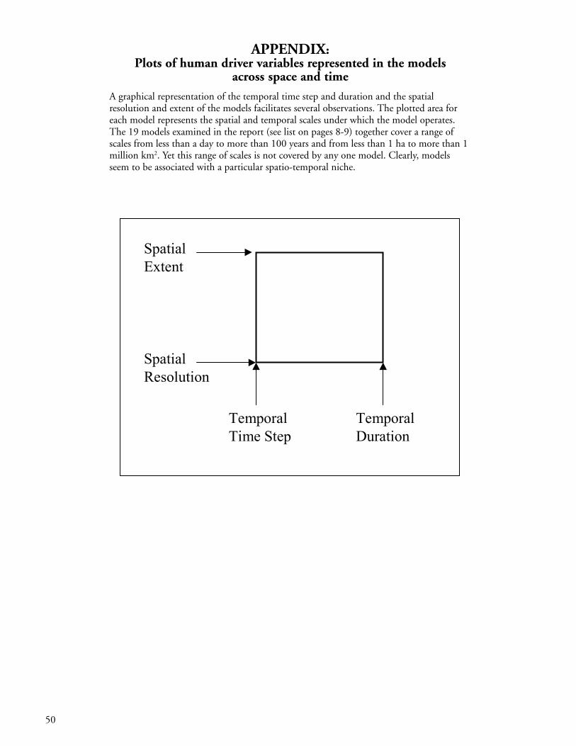
50
APPENDIX:Plots of human driver variables represented in the models
across space and time
A graphical representation of the temporal time step and duration and the spatialresolution and extent of the models facilitates several observations. The plotted area foreach model represents the spatial and temporal scales under which the model operates.The 19 models examined in the report (see list on pages 8-9) together cover a range ofscales from less than a day to more than 100 years and from less than 1 ha to more than 1million km2. Yet this range of scales is not covered by any one model. Clearly, modelsseem to be associated with a particular spatio-temporal niche.
SpatialExtent
SpatialResolution
TemporalTime Step
TemporalDuration

51
19
14
12
Temporal Scale [days]
Spat
ial S
cale
[m2 ]
Plot
Site
L
ands
cape
L
ocat
ion
R
egio
nal
Glo
bal
Hourly Daily Monthly Yearly Decadal Centennial
3 & 4
8
0.1 1 10 100 1000 10,000 100,000(1 week) (1 month) (1 year) (10 years) (100 years)
1
100
10,000
1,000,000
100,000,000
10,000,000,000
1,000,000,000,000
100,000,000,000,000
(1 km2)
(100 km2)
(10,000 km2)
(100 x 106 km2)
(1 ha)
(1 x 10⁶ km2)
79
106
11
5 States
Pixel / Stand
County/watershed
Landsat scene
Tree
U.S.A
17
13
6
2
11
151
18
1615
5
Farm
Cross-Sectional
Cross-Sectional
Human Drivers or Social Patterns and Preferences Model Variables
Population Size
19
14
12
Temporal Scale [days]
Spat
ial S
cale
[m2 ]
Plot
Site
L
ands
cape
L
ocat
ion
R
egio
nal
Glo
bal
Hourly Daily Monthly Yearly Decadal Centennial
3 & 4
8
0.1 1 10 100 1000 10,000 100,000(1 week) (1 month) (1 year) (10 years) (100 years)
1
100
10,000
1,000,000
100,000,000
10,000,000,000
1,000,000,000,000
100,000,000,000,000
(1 km2)
(100 km2)
(10,000 km2)
(100 x 106 km2)
(1 ha)
(1 x 10⁶ km2)
79
106
11
5 States
Pixel / Stand
County/watershed
Landsat scene
Tree
U.S.A
17
13
6
2
11
151
18
1615
5
Farm
Cross-Sectional
Cross-Sectional
Human Drivers or Social Patterns and Preferences Model Variables
Population Growth

52
19
14
12
Temporal Scale [days]
Spat
ial S
cale
[m2 ]
Plot
Site
L
ands
cape
L
ocat
ion
R
egio
nal
Glo
bal
Hourly Daily Monthly Yearly Decadal Centennial
3 & 4
8
0.1 1 10 100 1000 10,000 100,000(1 week) (1 month) (1 year) (10 years) (100 years)
1
100
10,000
1,000,000
100,000,000
10,000,000,000
1,000,000,000,000
100,000,000,000,000
(1 km2)
(100 km2)
(10,000 km2)
(100 x 106 km2)
(1 ha)
(1 x 10⁶ km2)
79
106
11
5 States
Pixel / Stand
County/watershed
Landsat scene
Tree
U.S.A
17
13
6
2
11
151
18
1615
5
Farm
Cross-Sectional
Cross-Sectional
Human Drivers or Social Patterns and Preferences Model Variables
Population Density
19
14
12
Temporal Scale [days]
Spat
ial S
cale
[m2 ]
Plot
Site
L
ands
cape
L
ocat
ion
R
egio
nal
Glo
bal
Hourly Daily Monthly Yearly Decadal Centennial
3 & 4
8
0.1 1 10 100 1000 10,000 100,000(1 week) (1 month) (1 year) (10 years) (100 years)
1
100
10,000
1,000,000
100,000,000
10,000,000,000
1,000,000,000,000
100,000,000,000,000
(1 km2)
(100 km2)
(10,000 km2)
(100 x 106 km2)
(1 ha)
(1 x 10⁶ km2)
79
106
11
5 States
Pixel / Stand
County/watershed
Landsat scene
Tree
U.S.A
17
13
6
2
11
151
18
1615
5
Farm
Cross-Sectional
Cross-Sectional
Human Drivers or Social Patterns and Preferences Model Variables
Returns to Land Use(Costs and Prices)

53
19
14
12
Temporal Scale [days]
Spat
ial S
cale
[m2 ]
Plot
Site
L
ands
cape
L
ocat
ion
R
egio
nal
Glo
bal
Hourly Daily Monthly Yearly Decadal Centennial
3 & 4
8
0.1 1 10 100 1000 10,000 100,000(1 week) (1 month) (1 year) (10 years) (100 years)
1
100
10,000
1,000,000
100,000,000
10,000,000,000
1,000,000,000,000
100,000,000,000,000
(1 km2)
(100 km2)
(10,000 km2)
(100 x 106 km2)
(1 ha)
(1 x 10⁶ km2)
79
106
11
5 States
Pixel / Stand
County/watershed
Landsat scene
Tree
U.S.A
17
13
6
2
11
151
18
1615
5
Farm
Cross-Sectional
Cross-Sectional
Human Drivers or Social Patterns and Preferences Model Variables
Job Growth
19
14
12
Temporal Scale [days]
Spat
ial S
cale
[m2 ]
Plot
Site
L
ands
cape
L
ocat
ion
R
egio
nal
Glo
bal
Hourly Daily Monthly Yearly Decadal Centennial
3 & 4
8
0.1 1 10 100 1000 10,000 100,000(1 week) (1 month) (1 year) (10 years) (100 years)
1
100
10,000
1,000,000
100,000,000
10,000,000,000
1,000,000,000,000
100,000,000,000,000
(1 km2)
(100 km2)
(10,000 km2)
(100 x 106 km2)
(1 ha)
(1 x 10⁶ km2)
79
106
11
5 States
Pixel / Stand
County/watershed
Landsat scene
Tree
U.S.A
17
13
6
2
11
151
18
1615
5
Farm
Cross-Sectional
Cross-Sectional
Human Drivers or Social Patterns and Preferences Model Variables
Costs of Conversion

54
19
14
12
Temporal Scale [days]
Spat
ial S
cale
[m2 ]
Plot
Site
L
ands
cape
L
ocat
ion
R
egio
nal
Glo
bal
Hourly Daily Monthly Yearly Decadal Centennial
3 & 4
8
0.1 1 10 100 1000 10,000 100,000(1 week) (1 month) (1 year) (10 years) (100 years)
1
100
10,000
1,000,000
100,000,000
10,000,000,000
1,000,000,000,000
100,000,000,000,000
(1 km2)
(100 km2)
(10,000 km2)
(100 x 106 km2)
(1 ha)
(1 x 10⁶ km2)
79
106
11
5 States
Pixel / Stand
County/watershed
Landsat scene
Tree
U.S.A
17
13
6
2
11
151
18
1615
5
Farm
Cross-Sectional
Cross-Sectional
Human Drivers or Social Patterns and Preferences Model Variables
Rent
Not 4
19
14
12
Temporal Scale [days]
Spat
ial S
cale
[m2 ]
Plot
Site
L
ands
cape
L
ocat
ion
R
egio
nal
Glo
bal
Hourly Daily Monthly Yearly Decadal Centennial
3 & 4
8
0.1 1 10 100 1000 10,000 100,000(1 week) (1 month) (1 year) (10 years) (100 years)
1
100
10,000
1,000,000
100,000,000
10,000,000,000
1,000,000,000,000
100,000,000,000,000
(1 km2)
(100 km2)
(10,000 km2)
(100 x 106 km2)
(1 ha)
(1 x 10⁶ km2)
79
106
11
5 States
Pixel / Stand
County/watershed
Landsat scene
Tree
U.S.A
17
13
6
2
11
151
18
1615
5
Farm
Cross-Sectional
Cross-Sectional
Human Drivers or Social Patterns and Preferences Model Variables
Collective Rule Making:Zoning

55
19
14
12
Temporal Scale [days]
Spat
ial S
cale
[m2 ]
Plot
Site
L
ands
cape
L
ocat
ion
R
egio
nal
Glo
bal
Hourly Daily Monthly Yearly Decadal Centennial
3 & 4
8
0.1 1 10 100 1000 10,000 100,000(1 week) (1 month) (1 year) (10 years) (100 years)
1
100
10,000
1,000,000
100,000,000
10,000,000,000
1,000,000,000,000
100,000,000,000,000
(1 km2)
(100 km2)
(10,000 km2)
(100 x 106 km2)
(1 ha)
(1 x 10⁶ km2)
79
106
11
5 States
Pixel / Stand
County/watershed
Landsat scene
Tree
U.S.A
17
13
6
2
11
151
18
1615
5
Farm
Cross-Sectional
Cross-Sectional
Human Drivers or Social Patterns and Preferences Model Variables
Collective Rule Making:Tenure
19
14
12
Temporal Scale [days]
Spat
ial S
cale
[m2 ]
Plot
Site
L
ands
cape
L
ocat
ion
R
egio
nal
Glo
bal
Hourly Daily Monthly Yearly Decadal Centennial
3 & 4
8
0.1 1 10 100 1000 10,000 100,000(1 week) (1 month) (1 year) (10 years) (100 years)
1
100
10,000
1,000,000
100,000,000
10,000,000,000
1,000,000,000,000
100,000,000,000,000
(1 km2)
(100 km2)
(10,000 km2)
(100 x 106 km2)
(1 ha)
(1 x 10⁶ km2)
79
106
11
5 States
Pixel / Stand
County/watershed
Landsat scene
Tree
U.S.A
17
13
6
2
11
151
18
1615
5
Farm
Cross-Sectional
Cross-Sectional
Human Drivers or Social Patterns and Preferences Model Variables
Infrastructure/AccessibilityDistance from Road

56
19
14
12
Temporal Scale [days]
Spat
ial S
cale
[m2 ]
Plot
Site
L
ands
cape
L
ocat
ion
R
egio
nal
Glo
bal
Hourly Daily Monthly Yearly Decadal Centennial
3 & 4
8
0.1 1 10 100 1000 10,000 100,000(1 week) (1 month) (1 year) (10 years) (100 years)
1
100
10,000
1,000,000
100,000,000
10,000,000,000
1,000,000,000,000
100,000,000,000,000
(1 km2)
(100 km2)
(10,000 km2)
(100 x 106 km2)
(1 ha)
(1 x 10⁶ km2)
79
106
11
5 States
Pixel / Stand
County/watershed
Landsat scene
Tree
U.S.A
17
13
6
2
11
151
18
1615
5
Farm
Cross-Sectional
Cross-Sectional
Human Drivers or Social Patterns and Preferences Model Variables
Infrastructure/AccessibilityDistance from Town/Market
19
14
12
Temporal Scale [days]
Spat
ial S
cale
[m2 ]
Plot
Site
L
ands
cape
L
ocat
ion
R
egio
nal
Glo
bal
Hourly Daily Monthly Yearly Decadal Centennial
3 & 4
8
0.1 1 10 100 1000 10,000 100,000(1 week) (1 month) (1 year) (10 years) (100 years)
1
100
10,000
1,000,000
100,000,000
10,000,000,000
1,000,000,000,000
100,000,000,000,000
(1 km2)
(100 km2)
(10,000 km2)
(100 x 106 km2)
(1 ha)
(1 x 10⁶ km2)
79
106
11
5 States
Pixel / Stand
County/watershed
Landsat scene
Tree
U.S.A
17
13
6
2
11
151
18
1615
5
Farm
Cross-Sectional
Cross-Sectional
Human Drivers or Social Patterns and Preferences Model Variables
Infrastructure/AccessibilityDistance from Village/Settlement

57
19
14
12
Temporal Scale [days]
Spat
ial S
cale
[m2 ]
Plot
Site
L
ands
cape
L
ocat
ion
R
egio
nal
Glo
bal
Hourly Daily Monthly Yearly Decadal Centennial
3 & 4
8
0.1 1 10 100 1000 10,000 100,000(1 week) (1 month) (1 year) (10 years) (100 years)
1
100
10,000
1,000,000
100,000,000
10,000,000,000
1,000,000,000,000
100,000,000,000,000
(1 km2)
(100 km2)
(10,000 km2)
(100 x 106 km2)
(1 ha)
(1 x 10⁶ km2)
79
106
11
5 States
Pixel / Stand
County/watershed
Landsat scene
Tree
U.S.A
17
13
6
2
11
151
18
1615
5
Farm
Cross-Sectional
Cross-Sectional
Human Drivers or Social Patterns and Preferences Model Variables
Infrastructure/AccessibilityPresence of Irrigation
19
14
12
Temporal Scale [days]
Spat
ial S
cale
[m2 ]
Plot
Site
L
ands
cape
L
ocat
ion
R
egio
nal
Glo
bal
Hourly Daily Monthly Yearly Decadal Centennial
3 & 4
8
0.1 1 10 100 1000 10,000 100,000(1 week) (1 month) (1 year) (10 years) (100 years)
1
100
10,000
1,000,000
100,000,000
10,000,000,000
1,000,000,000,000
100,000,000,000,000
(1 km2)
(100 km2)
(10,000 km2)
(100 x 106 km2)
(1 ha)
(1 x 10⁶ km2)
79
106
11
5 States
Pixel / Stand
County/watershed
Landsat scene
Tree
U.S.A
17
13
6
2
11
151
18
1615
5
Farm
Cross-Sectional
Cross-Sectional
Human Drivers or Social Patterns and Preferences Model Variables
Infrastructure/AccessibilityGeneralized Access Variable

58
19
14
12
Temporal Scale [days]
Spat
ial S
cale
[m2 ]
Plot
Site
L
ands
cape
L
ocat
ion
R
egio
nal
Glo
bal
Hourly Daily Monthly Yearly Decadal Centennial
3 & 4
8
0.1 1 10 100 1000 10,000 100,000(1 week) (1 month) (1 year) (10 years) (100 years)
1
100
10,000
1,000,000
100,000,000
10,000,000,000
1,000,000,000,000
100,000,000,000,000
(1 km2)
(100 km2)
(10,000 km2)
(100 x 106 km2)
(1 ha)
(1 x 10⁶ km2)
79
106
11
5 States
Pixel / Stand
County/watershed
Landsat scene
Tree
U.S.A
17
13
6
2
11
151
18
1615
5
Farm
Cross-Sectional
Cross-Sectional
Human Drivers or Social Patterns and Preferences Model Variables
Village Size
19
14
12
Temporal Scale [days]
Spat
ial S
cale
[m2 ]
Plot
Site
L
ands
cape
L
ocat
ion
R
egio
nal
Glo
bal
Hourly Daily Monthly Yearly Decadal Centennial
3 & 4
8
0.1 1 10 100 1000 10,000 100,000(1 week) (1 month) (1 year) (10 years) (100 years)
1
100
10,000
1,000,000
100,000,000
10,000,000,000
1,000,000,000,000
100,000,000,000,000
(1 km2)
(100 km2)
(10,000 km2)
(100 x 106 km2)
(1 ha)
(1 x 10⁶ km2)
79
106
11
5 States
Pixel / Stand
County/watershed
Landsat scene
Tree
U.S.A
17
13
6
2
11
151
18
1615
5
Farm
Cross-Sectional
Cross-Sectional
Human Drivers or Social Patterns and Preferences Model Variables
Silviculture andAgriculture

59
19
14
12
Temporal Scale [days]
Spat
ial S
cale
[m2 ]
Plot
Site
L
ands
cape
L
ocat
ion
R
egio
nal
Glo
bal
Hourly Daily Monthly Yearly Decadal Centennial
3 & 4
8
0.1 1 10 100 1000 10,000 100,000(1 week) (1 month) (1 year) (10 years) (100 years)
1
100
10,000
1,000,000
100,000,000
10,000,000,000
1,000,000,000,000
100,000,000,000,000
(1 km2)
(100 km2)
(10,000 km2)
(100 x 106 km2)
(1 ha)
(1 x 10⁶ km2)
79
106
11
5 States
Pixel / Stand
County/watershed
Landsat scene
Tree
U.S.A
17
13
6
2
11
151
18
1615
5
Farm
Cross-Sectional
Cross-Sectional
Human Drivers or Social Patterns and Preferences Model Variables
Technology Level
19
14
12
Temporal Scale [days]
Spat
ial S
cale
[m2 ]
Plot
Site
L
ands
cape
L
ocat
ion
R
egio
nal
Glo
bal
Hourly Daily Monthly Yearly Decadal Centennial
3 & 4
8
0.1 1 10 100 1000 10,000 100,000(1 week) (1 month) (1 year) (10 years) (100 years)
1
100
10,000
1,000,000
100,000,000
10,000,000,000
1,000,000,000,000
100,000,000,000,000
(1 km2)
(100 km2)
(10,000 km2)
(100 x 106 km2)
(1 ha)
(1 x 10⁶ km2)
79
106
11
5 States
Pixel / Stand
County/watershed
Landsat scene
Tree
U.S.A
17
13
6
2
11
151
18
1615
5
Farm
Cross-Sectional
Cross-Sectional
Human Drivers or Social Patterns and Preferences Model Variables
Affluence

60
19
14
12
Temporal Scale [days]
Spat
ial S
cale
[m2 ]
Plot
Site
L
ands
cape
L
ocat
ion
R
egio
nal
Glo
bal
Hourly Daily Monthly Yearly Decadal Centennial
3 & 4
8
0.1 1 10 100 1000 10,000 100,000(1 week) (1 month) (1 year) (10 years) (100 years)
1
100
10,000
1,000,000
100,000,000
10,000,000,000
1,000,000,000,000
100,000,000,000,000
(1 km2)
(100 km2)
(10,000 km2)
(100 x 106 km2)
(1 ha)
(1 x 10⁶ km2)
79
106
11
5 States
Pixel / Stand
County/watershed
Landsat scene
Tree
U.S.A
17
13
6
2
11
151
18
1615
5
Farm
Cross-Sectional
Cross-Sectional
Human Drivers or Social Patterns and Preferences Model Variables
Age
19
14
12
Temporal Scale [days]
Spat
ial S
cale
[m2 ]
Plot
Site
L
ands
cape
L
ocat
ion
R
egio
nal
Glo
bal
Hourly Daily Monthly Yearly Decadal Centennial
3 & 4
8
0.1 1 10 100 1000 10,000 100,000(1 week) (1 month) (1 year) (10 years) (100 years)
1
100
10,000
1,000,000
100,000,000
10,000,000,000
1,000,000,000,000
100,000,000,000,000
(1 km2)
(100 km2)
(10,000 km2)
(100 x 106 km2)
(1 ha)
(1 x 10⁶ km2)
79
106
11
5 States
Pixel / Stand
County/watershed
Landsat scene
Tree
U.S.A
17
13
6
2
11
151
18
1615
5
Farm
Cross-Sectional
Cross-Sectional
Human Drivers or Social Patterns and Preferences Model Variables
Human Attitudes and Values& Food Security

61
GlossaryArea base model: Allocates proportions of a given landbase to predefined land-use categories.
Complexity: In this paper we refer to three types ofcomplexity—spatial, temporal, and humandecisionmaking—all of which are defined in thisGlossary.
Conceptual model: Theoretical description ofsocioeconomic and physical processes.
Control (or flow) variables: System elements thatrepresent the action or change in a state.
Discrete finite state model: Model that is discrete (spacerepresented as cells or blocks) and finite state (representsan object as being in only a few, finite number of states orconditions).
Duration: The length of time for which the model isapplied. The duration of a model’s results may bereported as the number of time steps used (e.g., 100annual times steps), the period of the model (100 years),or the model dates (January 1, 1900, to January 1, 2000).
Dynamic systems model: Systems models that attemptto capture changes in real or simulated time.
Extent: The total geographic area to which the model isapplied.
Human decisionmaking: How models incorporatehuman elements. Human decisionmaking sections ofmodels vary in terms their theoretical precursors and maybe simply linked deterministically to a set ofsocioeconomic or biological drivers, or may be based onsome game theoretic or economic models. Threeattributes of human decisionmaking that are important toconsider in thinking about diverse models of land-usechange are complexity, jurisdictional domain, andtemporal range.
Human decisionmaking (HDM) complexity: Thespecificity and detailed consideration given in a model tothe decisions that humans make that affect land-usechange. For this exercise, we have developed a scale ofcomplexity that ranges from 1 to 6.
Jurisdictional domain: The spatial scope of humandecisionmaking. If desired, a jurisdictional domain maybe split up to reflect resolution, the decisionmakingdomain for a particular actor, and to reflect spatial extent,in this case the total area over which the actor(s) has(have)influence, or the jurisdictional range.
Linear planning model: Model that optimizes a linearfunction subject to several linear constraints, expressed aslinear inequalities or equalities.
Markov model: A probabilistic modeling method wheremodel state outcomes rely strictly on previous model
states. With this modeling technique, cell conditionalprobabilities are used to change cell states through a seriesof iterative operations.
Resolution: The smallest spatial unit of analysis for themodel. For example, in a raster or grid representation ofthe landscape, each unit or cell area is usually treated as aconstant size.
Spatial complexity: The presence of a spatial componentof a model or information. Spatial complexity may berepresentative or interactive.
Spatial dynamic model: Models that are spatially explicitand dynamic.
Spatial interaction: Models are based on topologicalrelationships. Topology is a mathematical procedure fordefining spatial relationships, usually as lists of features,and using the concepts of connectivity, area definition,and contiguity.
Spatial Markov model: Spatially explicit model thatcarries over memory from one state to the next, butusually from only the last state; e.g., the probability thatthe system will be in a given state (land class) at sometime t
2, is deduced from the knowledge of its state at time
t1.
Spatial representation: Spatially representative modelsare able to display data as maps but do not includetopology and spatial interactions.
Spatial stochastic model: Spatially explicit model that isinteractive and incorporates random changes todetermine transition probabilities from one land cover toanother.
State variables: Elements that make up the system forwhich the model is being developed.
Temporal complexity: A model’s ability to handle a largenumber of time steps, time lags, and feedback responses.
Time step: The smallest temporal unit of analysis of themodel variable.
von Thünen: German landowner Johann Heinrich vonThünen developed a model that relates intensity and typeof land use to transportation costs and land rent. Themodel (published in The Isolated State, 1826) involves ahomogenous plane within which exists an isolated city.Land-use patterns around this city are a function of travelcost to the city. Land uses producing goods with arelatively high transportation cost (e.g., perishable orheavy products) would be produced close to the city, andland uses producing more durable goods (with lowertransportation costs) would be produced farther from thecity. This arrangement results in a series of different land-use zones around the city. Many authors have applied andexpanded upon von Thünen’s initial theory (e.g.,Papageorgiou 1990).

Printed on Recycled Paper
Agarwal, Chetan; Green, Glen M.; Grove, J. Morgan; Evans, Tom P.; Schweik, Charles M.2002. A review and assessment of land-use change models: dynamics of space,time, and human choice. Gen. Tech. Rep. NE-297. Newtown Square, PA: U.S.Department of Agriculture, Forest Service, Northeastern Research Station. 61 p.
A review of different types of land-use change models incorporating human processes.Presents a framework to compare land-use change models in terms of scale (both spatialand temporal) and complexity, and how well they incorporate space, time, and humandecisionmaking. Examines a summary set of 250 relevant citations and develops abibliography of 136 papers. From these papers, 19 land-use models are reviewed indetail as representative of the broader set of models. Summarizes and discusses the 19models in terms of dynamic (temporal) and spatial interactions, as well as humandecisionmaking. Many raster models examined mirror the extent and resolution ofremote-sensing data. The broadest-scale models generally are not spatially explicit.Models incorporating higher levels of human decisionmaking are more centrally locatedwith respect to spatial and temporal scales, probably due to the lack of data availability atmore extreme scales. Examines the social drivers of land-use change and methodologicaltrends and concludes with some proposals for future directions in land-use modeling.
Keywords: cellular automata, dynamic model, GIS, human decisionmaking, human-environment, land cover, LUCC, model comparison, model modularity, spatial model
Published by: For additional copies:
USDA FOREST SERVICE USDA Forest Service11 CAMPUS BLVD SUITE 200 Publications DistributionNEWTOWN SQUARE PA 19073-3294 359 Main Road
Delaware, OH 43015-8640November 2002 Fax: (740)368-0152
Visit our homepage at: http://www.fs.fed.us/ne
Manuscript received for publication 9 July 2001

Headquarters of the Northeastern Research Station is in Newtown Square,Pennsylvania. Field laboratories are maintained at:
Amherst, Massachusetts, in cooperation with the University of Massachusetts
Burlington, Vermont, in cooperation with the University of Vermont
Delaware, Ohio
Durham, New Hampshire, in cooperation with the University of New Hampshire
Hamden, Connecticut, in cooperation with Yale University
Morgantown, West Virginia, in cooperation with West Virginia University
Parsons, West Virginia
Princeton, West Virginia
Syracuse, New York, in cooperation with the State University of New York,College of Environmental Sciences and Forestry at Syracuse University
Warren, Pennsylvania
The U. S. Department of Agriculture (USDA) prohibits discrimination in all its programs andactivities on the basis of race, color, national origin, gender, religion, age, disability, politicalbeliefs, sexual orientation, and marital or family status. (Not all prohibited bases apply to allprograms.) Persons with disabilities who require alternative means for communication ofprogram information (Braille, large print, audiotape, etc.) should contact the USDA's TARGETCenter at (202)720-2600 (voice and TDD).
To file a complaint of discrimination, write USDA, Director, Office of Civil Rights, Room 326-W,Whitten Building, 14th and Independence Avenue SW, Washington, DC 20250-9410, or call(202)720-5964 (voice and TDD). USDA is an equal opportunity provider and employer.
“Ca“Ca“Ca“Ca“Carrrrring for the Land and Seing for the Land and Seing for the Land and Seing for the Land and Seing for the Land and Serrrrrving People Thrving People Thrving People Thrving People Thrving People Through Reseaough Reseaough Reseaough Reseaough Researrrrrch”ch”ch”ch”ch”