a renormalization group primer - welcome to scipp

A Renormalization Group Primer

Physics 295 2010. Independent Study.Topics in Quantum Field Theory

Michael DineDepartment of Physics

University of California, Santa Cruz

May 2010

Physics 295 2010. Independent Study. Topics in Quantum Field TheoryA Renormalization Group Primer

Introduction: Some Simple Dimensional Analysis

Consider a theory with only massless fields, or at energy andmomentum scales so large that all masses may be neglected.In this case, one might think that one could determine thestructure of any amplitude purely by dimensional analysis. Forexample, at high energies in QED, one might guess that theamplitude for elastic electron-electron scattering would take theform:

A(q) =f (e2)

q2 (1)

where f (e2) is some dimensionless function of thedimensionless variable e2, which one might compute order byorder in perturbation theory, or in some other way.


But we know that this isn’t quite right, once one takes intoaccount the ultraviolet divergences in the theory. Inperturbation theory, amplitudes depend also on logarithms ofq/µ2, where µ is a renormalization scale.


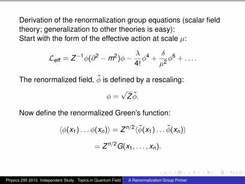
Derivation of the renormalization group equations (scalar fieldtheory; generalization to other theories is easy):Start with the form of the effective action at scale µ:

Leff = Z−1φ(∂2 −m2)φ− λ

4!φ4 +

δ

µ2φ6 + . . . .

The renormalized field, φ is defined by a rescaling:

φ =√

Z φ.

Now define the renormalized Green’s function:

〈φ(x1) . . . φ(xn)〉 = Z n/2〈φ(x1) . . . φ(xn)〉

= Z n/2G(x1, . . . , xn).


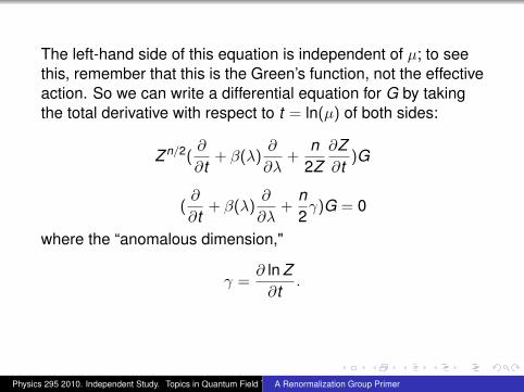
The left-hand side of this equation is independent of µ; to seethis, remember that this is the Green’s function, not the effectiveaction. So we can write a differential equation for G by takingthe total derivative with respect to t = ln(µ) of both sides:

Z n/2(∂

∂t+ β(λ)

∂

∂λ+

n2Z

∂Z∂t

)G

(∂

∂t+ β(λ)

∂

∂λ+

n2γ)G = 0

where the “anomalous dimension,"

γ =∂ ln Z∂t

.


This equation is known as the Callan-Szymanzik equation. Wecan obtain what is known as the “renormalization group"equation by dimensional analysis. Suppose we are interestedin a Green’s function in momentum space, G(p1, . . .pn).Suppose also that all of the (Euclidean) momentum invariantsare comparable, i.e.

p2i = x2

i M2; pi · pj = xijM2; xi , xij = O(1).

We can determine how G depends on M. Define

t = ln(µ2/M2).

Here we are using the fact that by dimensional analysis, all Mdependence is related to µ-dependence. It is convenient, if Ghas naive dimension −d , to take

G = M−d f (t , xi , xij).


Then f satisfies (why?)

(∂

∂t+ β(λ)

∂

∂λ+

n2γ)f = 0

The solution can be found by the fluid mechanics analogy, orsimply by making a good guess. Define the running couplingconstant

λ(t) :∂λ(t)∂t

= β(λ(t)).

Then

f (t , λ,M) = f (λ(t))e−∫ λ

λon2

γ(λ′)β(λ′) dλ′

.

Plugging in, one can see that this satisfies the original equation.


One can consider, instead, the renormalization group equationfor terms in the effective action. Returning to the effectiveaction for φ, after the rescaling,

Leff =12φ(∂2 −m2)φ− Z 4/2 λ

4!φ4 + Z 6/2 δ

µ2φ6 + . . . .

The Z factors are just what are required to renormalize thecouplings, i.e. the terms in the effective action can be written interms of the renormalized couplings, plus explicit cutoff and µdependence in the original one-particle irreducible diagram (theµ-dependence can be thought of as arising from thecounterterm).


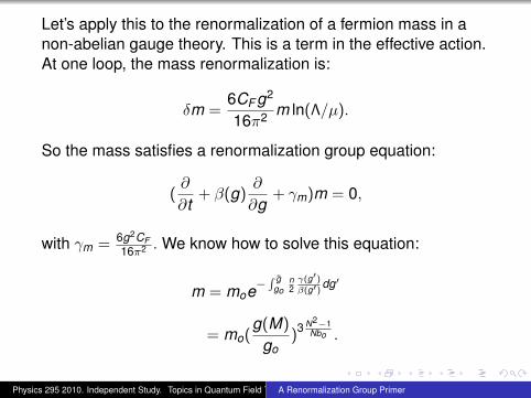
Let’s apply this to the renormalization of a fermion mass in anon-abelian gauge theory. This is a term in the effective action.At one loop, the mass renormalization is:

δm =6CF g2

16π2 m ln(Λ/µ).

So the mass satisfies a renormalization group equation:

(∂

∂t+ β(g)

∂

∂g+ γm)m = 0,

with γm = 6g2CF16π2 . We know how to solve this equation:

m = moe−∫ g

gon2

γ(g′)β(g′) dg′

= mo(g(M)

go)3 N2−1

Nbo .


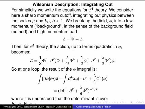
Wilsonian Description: Integrating OutFor simplicity we write the equations for φ4 theory. We considerhere a sharp momentum cutoff, integrating out physics betweenthe scales µ and bµ, b < 1. We break up the field, φ, into a lowmomentum (“background", in the sense of the background fieldmethod) and high momentum part:

φ = Φ + φ

Then, for φ4 theory, the action, up to terms quadratic in φ,becomes:

L =12

Φ(−∂2)Φ +λ

4!Φ4 +

12φ(−∂2 +

λ

2Φ2)φ.

So at one loop, the result of the φ integral is:∫[dφ]exp(−

∫d4xφ(−∂2 +

λ

4Φ2)φ)

= det(−∂2 +λ

4Φ2)−1/2

where it is understood that the determinant is overbµ < |k | < µ.


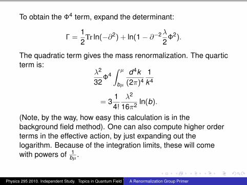
To obtain the Φ4 term, expand the determinant:

Γ =12

Tr ln(−∂2) + ln(1− ∂−2λ

2Φ2).

The quadratic term gives the mass renormalization. The quarticterm is:

λ2

32Φ4∫ µ

bµ

d4k(2π)4

1k4

= 314!

λ2

16π2 ln(b).

(Note, by the way, how easy this calculation is in thebackground field method). One can also compute higher orderterms in the effective action, by just expanding out thelogarithm. Because of the integration limits, these will comewith powers of 1

bµ .


At this order, the effective action has the structure:

Γ =

∫d4x(

12∂Φ2−1

2m2Φ2− 1

4!(λ(1− 3

32π2 ) ln(b))Φ4+1µ2 Φ6+. . . )

It comes with cutoff bµ. We can change this to a theory with afixed cutoff by introducing k = k ′b, x = x ′

b . In terms of these,the cutoff is µ, and the lagrangian has extra factors of b:

Γ =

∫d4x ′(

b−2

2∂Φ2 − b−4

2m2Φ2

−b−4

4!(λ(1− 3

32π2 ) ln(b))Φ4 + b−4 1µ2 Φ6 + . . . )


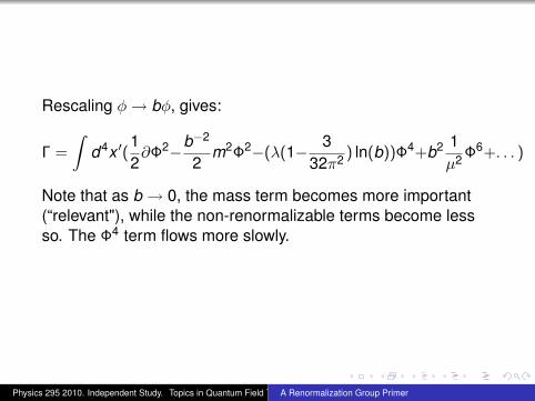
Rescaling φ→ bφ, gives:

Γ =

∫d4x ′(

12∂Φ2−b−2

2m2Φ2−(λ(1− 3

32π2 ) ln(b))Φ4+b2 1µ2 Φ6+. . . )

Note that as b → 0, the mass term becomes more important(“relevant"), while the non-renormalizable terms become lessso. The Φ4 term flows more slowly.


Fixed Points

Suppose the β function has a zero, as indicated in the figure:

β = ±C(g − go).

Then the running coupling is given by:

g − go = e±C(t).

So the running coupling goes to the fixed point either ast = ln(µ/p)→ ∓∞. These are referred to, accordingly, asultraviolet or infrared fixed points. Operators of a givenanomalous dimension then tend to zero at the fixed points withpowers of p different than expected from classical dimensionalanalysis. This is the origin of the term “anomalous dimension."


The “Banks-Zaks" Fixed PointIn condensed matter physics, such conformal fixed points areimportant in critical phenomena in range of systems, withvarying dimensionality. This is discussed in chapter 13 of yourtext. There are now also a wide range of four dimensional fieldtheories known with non-trivial conformal fixed points. This hasemerged from the work of Seiberg; the theories of this sortwhich are understood are supersymmetric (at some point, if wedo a supersymmetry course, we can discuss this).


But there is a simple class of theories where a fixed point canbe found in perturbation theory. For these, we consider theorieswith a large number of colors and flavors. It is simplest toconsider here also the supersymmetric case. Then, to two looporder, the beta function is given by:

bo = −(3N−Nf )g3

16π2 b1 = −[6N2−2NNf−4NfN2 − 1

2N](

g2

16π2 )2g.

(2)Vanishing of the beta function gives, to this order,

Nf = 3N − ε g∗2

16π2 =ε

6N2 . (3)

Here we will think of N as extremely large, and ε as an integerof order 1. There will be corrections to this result at higherorders in g. In particular, at higher orders, g∗ is schemedependent.


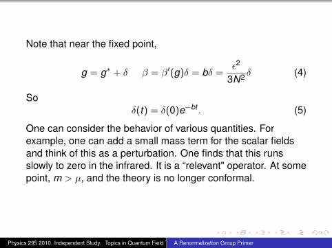
Note that near the fixed point,

g = g∗ + δ β = β′(g)δ = bδ =ε2

3N2 δ (4)

Soδ(t) = δ(0)e−bt . (5)

One can consider the behavior of various quantities. Forexample, one can add a small mass term for the scalar fieldsand think of this as a perturbation. One finds that this runsslowly to zero in the infrared. It is a “relevant" operator. At somepoint, m > µ, and the theory is no longer conformal.


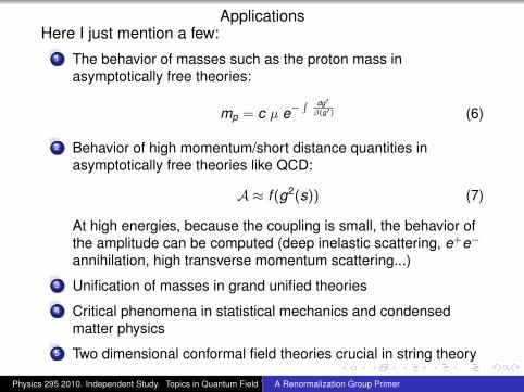
ApplicationsHere I just mention a few:

1 The behavior of masses such as the proton mass inasymptotically free theories:

mp = c µ e−∫ dg′

β(g′) (6)

2 Behavior of high momentum/short distance quantities inasymptotically free theories like QCD:

A ≈ f (g2(s)) (7)

At high energies, because the coupling is small, the behavior ofthe amplitude can be computed (deep inelastic scattering, e+e−

annihilation, high transverse momentum scattering...)

3 Unification of masses in grand unified theories

4 Critical phenomena in statistical mechanics and condensedmatter physics

5 Two dimensional conformal field theories crucial in string theory


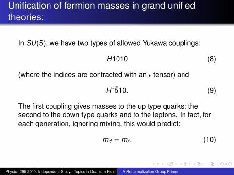
Unification of fermion masses in grand unifiedtheories:

In SU(5), we have two types of allowed Yukawa couplings:

H1010 (8)

(where the indices are contracted with an ε tensor) and

H∗510. (9)

The first coupling gives masses to the up type quarks; thesecond to the down type quarks and to the leptons. In fact, foreach generation, ignoring mixing, this would predict:

md = m`. (10)


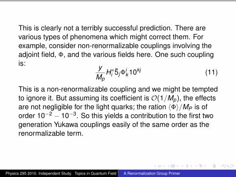
This is clearly not a terribly successful prediction. There arevarious types of phenomena which might correct them. Forexample, consider non-renormalizable couplings involving theadjoint field, Φ, and the various fields here. One such couplingis: y

MpH∗i 5jΦ

ik10kj (11)

This is a non-renormalizable coupling and we might be temptedto ignore it. But assuming its coefficient is O(1/Mp), the effectsare not negligible for the light quarks; the ration 〈Φ〉/MP is oforder 10−2 − 10−3. So this yields a contribution to the first twogeneration Yukawa couplings easily of the same order as therenormalizable term.


The third generation is more interesting. Here the tree levelrelation is not wildly off (a factor of three) and much work hasgone intro trying to understand this. As for the gauge couplings,we need to consider renormalization corrections. At very highenergies, much greater than the quark masses, we can treatthe mass terms as perturbative terms in the lagrangian, andstudy their renormalization and their evolution with scale.Indeed, we have already calculated the mass renormalization inQED. In the case of a non-abelian group, the result (for fermionsin the fundamental representation, i.e. for SU(3) or SU(2), inthe case of the b and the τ ) one just multiplies by 1/2, for thetrace of the fermion generators. So, in the effective action,integrating out physics between scale Λ and scale µ, we have

m0

(1 + 3/2

g2

16π2 ln(Λ2

µ2 )

)ψψ (12)

where the g is that appropriate to either b or τ .


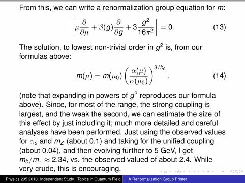
From this, we can write a renormalization group equation for m:[µ∂

∂µ+ β(g)

∂

∂g+ 3

g2

16π2

]= 0. (13)

The solution, to lowest non-trivial order in g2 is, from ourformulas above:

m(µ) = m(µ0)

(α(µ)

α(µ0)

)3/b0

. (14)

(note that expanding in powers of g2 reproduces our formulaabove). Since, for most of the range, the strong coupling islargest, and the weak the second, we can estimate the size ofthis effect by just including it; much more detailed and carefulanalyses have been performed. Just using the observed valuesfor αs and mZ (about 0.1) and taking for the unified coupling(about 0.04), and then evolving further to 5 GeV, I getmb/mτ ≈ 2.34, vs. the observed valued of about 2.4. Whilevery crude, this is encouraging.


a renormalization group primer - welcome to scipp

Documents