a real-time spatio-temporal data exploration tool for ... real-time spatio-temporal data exploration...
TRANSCRIPT

A real-time spatio-temporal
data exploration tool for marine research
Anthony David Veness
Master of Applied Science
University of Tasmania
A thesis submitted in partial fulfillment of the requirements for a Masters
Degree at the School of Geography and Environmental Studies,
Faculty of Science, Technology and Engineering, University of Tasmania
(October 2009)

ii
Declaration
This thesis contains no material which has been accepted for the award of any other degree
or diploma in any tertiary institution, and to the best of my knowledge and belief, contains
no material previously published or written by another person, except where due reference is
made in the text of the thesis.
Signed
Tony Veness
16th October 2009.

iii
ABSTRACT
The resources required to acquire high quality scientific data in a marine environment can be
great. The complication of acquiring data from a platform which pitches, rolls and heaves
makes the challenge even greater. The variability of the weather and sea conditions, along
with equipment failures, seemingly conspire against the marine scientist. There is a great
need for good quality-control measures, accurate electronic record keeping, and effective
voyage management at sea if a good outcome from an expensive sea voyage is to be
expected.
Typically, the plethora of navigation, data acquisition, quality control, Geographical
Information Systems and databases used at sea on the world’s research vessels do not allow
an intuitive, holistic, spatial and temporal view of real-time data. “How close are we to the
ship track from our last visit to the region?” or “What was the deployment depth of the
instrument when we were last at this site two years ago?” are typical questions asked by
those undertaking research far from shore. Answering these questions like these, in a timely
manner, using systems commonly used on research vessels can be difficult.
This study explored the combination of an open-source spatio-temporal DataBase
Management System (DBMS) and Keyhole Markup Language (KML), creating a framework
for the storage and exploration of real-time spatio-temporal data at sea. The framework
supported multiple concurrent users using Virtual Globe browsers. This study created a
methodology, which resulted in a functional software tool, MARVIN, using open-source
software.
Empirical and modelled datasets were used in conjunction with MARVIN, both at sea and in
the laboratory. MARVIN was found to be able to provide a simple and intuitive 4D (3D +
time) real-time view of spatio-temporal datasets, as they were collected at sea.
The key combination of a spatio-temporal DBMS and KML, offered a robust solution for the
storage of real-time data, undertaking of Geographical Information System (GIS) operations,
and streaming of data to multiple clients, running Virtual Globe browsers such as Google
Earth. The techniques implemented also support existing navigation, (3D) GIS, and numeric
modelling software commonly used on modern research vessels.
iv
Acknowledgments
I would like to thank my supervisor, Dr Arko Lucieer for his valued support and guidance
throughout the coursework and thesis components of my studies. Arko’s enthusiasm for
research and professional approach sets an example which I and others can only hope to
follow.
Dr Jon Osborn provided me with invaluable advice during my four years of part-time study
at the Centre for Spatial Information Science, University of Tasmania. His keen eye and
sound advice ensured I completed what I needed to complete, when I needed to complete it.
To my partner Jane, whose ability with a red pen is not to be taken lightly, I give many many
thanks and promise not to start a PhD, really..…

v
Table of Contents
Declaration……………………………………………………………………….…... Abstract………………………………………………………………………….…… Acknowledgements……………………………………………………………...…… Table of contents…………………………………………………………………..…. List of Figures…………………………………………………………………….….. List of Tables…………………………………………………………………….…... Chapter One – Introduction……………………………………………………...…
1.1 Motivation……………………………………………………………..… 1.2 Aims and Objectives…………………………………………….…….…
Chapter Two – Literature Review …………………………………………….…..
2.1 Technologies………………………………………………………….…. 2.1.1 Databases……………………………………………….…… 2.1.2 Web servers…………………………………………………. 2.1.3 Map and Geo servers…………………………………….…..
2.2 Mainstream methodologies………………………………………….…... 2.2.1 Server-side map generation……………………………….… 2.2.2 Client-side map generation……………………………….….
2.3 Virtual Globes…………………………………………………………… 2.4 Specialised 3D and 4D data visualisation software…………………..….
Chapter Three – Methods……………………………………………………….….
3.1 Introduction…………………………………………………………..….. 3.2 Hardware……………………………………………………….……..….
3.2.1 Server……………………………………………………..…. 3.2.2 Clients…………………………………………………….….
3.3 Software…………………………………………………………….…… 3.3.1 Database – PostgreSQL / PostGIS………………………..… 3.3.2 Web server - Apache HTTP……………………………….… 3.3.3 Server-side scripting languages - PHP and Python………..… 3.3.4 Server-side graphing package – JpGraph…………………..... 3.3.5 Server-side map server package – MapServer…………….… 3.3.6 Virtual Globe browser - Google Earth……………………....
3.4 Datasets……………………………………………………………….…. 3.4.1 Real-world collected datasets……………………………..…. 3.4.2 Simulated datasets…………………………………………....
3.5 Implementation………………………………………………………..…. 3.5.1 Overview…………………………………………………..…
ii
iii
iv
v
vii
viii
1
4 5
7
8 10 15 16 18 20 23 25 27
29
32 33 33 34 35 35 35 36 37 38 39 41 41 42 51 51
vi
3.5.2 DMBS……………………………………….………………. 3.5.3 Keyhole Markup Language………………………………..… 3.5.4 Temporary file use…………………………………………... 3.5.5 PHP Programs……………………………………………….. 3.5.6 Google Earth…………………………………………………
Chapter Four – Results……………………………………………………………...
4.1 Introduction to MARVIN…………………………….……………….…. 4.2 Real-time Vessel network link………………………………..…………. 4.3 Real-time Charts network link………………………………………..…. 4.4 Waypoints network link………………………………………..………... 4.5 Instruments network link………………………………………….……... 4.6 Historic Vessel Track network link………………………………….…... 4.7 Time Series network link………………………………………..………. 4.8 Scenarios…………………………………………………………………
4.8.1 Scenario 1: Distance measurement……………………….…. 4.8.2 Scenario 2: Determining CTD depth…………………….….. 4.8.3 Scenario 3: Determining camera sled position and time….…. 4.8.4 Scenario 4: Contaminated site………………….…………….
4.9 Summary………………………………………………………………… Chapter Five – Discussion…………………………………………………………..
5.1 Introduction……………………………………………………………… 5.2 MARVIN versus GIS software……………………………………….…. 5.3 MARVIN versus specialised 3D and 4D modelling software………...…
Chapter Six – Conclusion…………………………………………………………...
6.1 Major strengths…………………………………………………………... 6.2 Major challenges…………………..…………………………………….. 6.3 Future work………………………………………………………………
References…………………………………………………………………………… Abbreviations………………………….……………………………………...………
54 62 65 71 73
74
75 77 80 82 84 87 89 91 92 93 94 97
100
101
102 106 108
109
110 111 112
113
118

vii
List of Figures
Figure 2.1: Overview of OGC WMS method for server-side web mapping……….
Figure 2.2: Overview of a server-side web mapping system – MapServer………...
Figure 2.3: Overview of OGC WFS method for client-side mapping……………...
Figure 2.4: Generalised dataflows for a Google Earth based web mapping system..
Figure 3.1: Example of a time series graph generated by JpGraph…………………
Figure 3.2: MARVIN screen capture showing modelled MBES sonar beams……..
Figure 3.3: Sonardyne USBL Range Pro software screen capture…………………
Figure 3.4: Overview schematic of MARVIN major components…………………
Figure 3.5: MARVIN database schema…………………………………………….
Figure 3.6: Example COLLADA models used by MARVIN………………………
Figure 3.7: Example of JpGraph text images of real-time underway data………….
Figure 3.8: Example of JpGraph text images of historic underway data…………...
Figure 3.9: Examples of PHP Mapcsript generated planimetric chart images……...
Figure 3.10: MARVIN launcher KML file and PHP programs datapaths………….
Figure 3.11: MARVIN.kml…………………………………………………………
Figure 4.1: MARVIN’s six network link icons.………………………………...…..
Figure 4.2: Overview of MARVIN layers, as shown in the Google Earth side bar...
Figure 4.3: Real-time Vessel network link icons…………………………………...
Figure 4.4: Vessel model (small)…………………………………………………...
Figure 4.5: Vessel model (large)……………………………………………………
Figure 4.6: Modelled multi-beam echo-sounder beams…………………………….
Figure 4.7: Real-time Charts network link icons…………………………………...
Figure 4.8: Three simultaneous views of vessel position in MARVIN…………….
Figure 4.9: Waypoints network link icons………………………………………….
Figure 4.10: Example of a pop-up balloon and equipment path……………………
Figure 4.11: Examples of pop-up balloons supported in MARVIN……………….
Figure 4.12: Instruments network link icons……………………………………….
Figure 4.13: Determining instrument depth during a historic deployment…………
Figure 4.14: Historic Vessel network link icons……………………………………
Figure 4.15: Historic Vessel network link vessel track and drapes………………...
Figure 4.16: Time Series network link icons……………………………………….
Figure 4.17: 24 hour time series graphs and drapes………………………………... Figure 4.18: Scenario one: Determining distance…………………………………..
20
21
24
27
37
44
47
52
56
64
67
68
70
72
73
75
76
77
77
78
79
80
81
82
83
84
84
85
87
88
89
90
92

viii
Figure 4.19: Scenario two: Determining depth……………………………..……… Figure 4.20: Scenario three: Determining time…………………………………….. Figure 4.21: Scenario three: Determining time (small scale)……………………….
Figure 4.22: Scenario four: Determining spatial correlation……………………….
Figure 5.1: Screen capture of MARVIN showing full Google Earth window……...
Figure 5.2: uDig screen capture, accessing MARVIN database……………………
93
95
96
99
101
105
List of Tables
Table 2.1: A selection of DBMSs and supported geometry datatypes……………..
Table 3.1: MARVIN server computer specifications……………………………….
Table 3.2: Client computer specifications…………………………………………..
Table 3.3: MARVIN underway datasets details……………………………………
Table 3.4: Details of MARVIN PHP programs…………………………………….
15
33
34
42
71

1
Chapter 1 Introduction
The increase in recent years of the number of websites with mapping capabilities has been
great. Mitchell (2005) defines web mapping as the broad technique that allows access to
static or interactive digital maps via a web browser. Many scientific and research
organisations utilise some form of web mapping for presenting or exploring their collected
datasets or results via a map or (nautical) chart on their corporate websites. The ready
adoption by the general public of map based technologies such as ‘Where-Is’, ‘Google
Maps’, and ‘Tom-Tom’ is an illustration of the power of mapping technologies.
Most individuals appreciate the benefits of a clear and accurate up-to-date map when
undertaking a journey. The expert and laypersons’ increased ability to understand patterns
and phenomena, and draw conclusions, when spatial data are presented in a simple map or
chart form is widely accepted. A map can very usefully show where they have been, where
they are, and where they are going (Kraak, 2004). Distances and times can be calculated,
either accurately or implied, from observation and ‘rule of thumb’. Plans can be more easily
made, understood and changed, when a route is presented as a map, rather than as a table of
place names, coordinates and times.
Computer applications such as Google Earth (GE), NASA Worldwind and ESRI’s ArcGIS
Explorer allow the multi-user exploration of geographic data in intuitive ‘Virtual Globe’
(VG) environments. Rather than a flat or planimetric view of the Earth’s land surfaces and
oceans, much like a flat paper map or chart, a three dimensional (3D) globe view is created
on a two dimensional (2D) computer monitor. Elvidge et al. (2008) describe the ease at
which an on-screen Virtual Globes to be rotated and examined in the required detail, much
like a real desktop globe. Intuitive non-planimetric views of an area of interest have great
advantages when the elevations or depths of features are an important visualisation
requirement.
A marine research voyage leaving port for a one to two month sortie is undertaking a journey
of discovery in many respects. The typical scientist aboard the vessel will have prepared for
many months and in some cases years, for the day of departure. Careful pre-voyage plans
would have been made, detailing important information such as intended routes, locations
for planned instrument and net deployments, stationary periods while deploying or retrieving
instruments (on station) and transit speeds and times, for example.

2
A vital component in support of the discovery process is the careful observation and
measurement of the physical characteristics of phenomena of interest. On a modern research
vessel, the task of measuring and logging ‘underway’ parameters such as sea surface
temperature or wind direction is largely automated. Computer network based data
acquisition systems can acquire data from a wide variety of continuously recording
instruments. Data can be stored at pre-determined intervals into files on server hard drives
or into databases.
Importantly, the position of the vessel, and the time and date when the measurement was
taken, are associated with the data. Data collected from towed or vertically profiling
instruments such as Conductivity, Temperature and Depth instruments (CTD), weather
balloons and net mounted instruments are also generally stored digitally with associated
spatial and temporal information.
As well as storing underway data from vessel mounted sensors and data from deployed
underwater instruments, typical scientific vessel data acquisition, storage and display
systems, allow the storage of important ‘event’ data. Event data includes the times and
positions of planned and actual equipment deployment or retrievals (waypoints), animal
observations, or the opening and closing of fishing nets, for example. Typical in-house data
acquisition systems provide a range of customised event logging functions which can be
altered on voyage or a scientific program basis (Shields et al., 2001).
The position of the net when a trawl starts and stops allows the catch data to be assigned
position and depth attributes. The catch data may be determined within hours, or up to
several years after a trawl. Without reliable spatial and temporal meta-data, this catch data
may be of limited scientific use. The correct logging of event data during a long research
voyage with time and date (typically in UTC), and position (in three dimensions) is vital for
record keeping purposes and dynamic voyage planning.
The ability to undertake simple overlay functions in a mapping package or desktop
Geographical Information System (GIS) software cannot be undertaken unless the positions
and times of all important events throughout a research voyage are accurately logged.
Likewise, the synthesis of spatial datasets collected on a research voyage, with historic
datasets that can allow hypothesis testing, can only be undertaken using if positions and
times are accurately recorded.

3
Poor weather or equipment failures may require voyage management personnel to adapt the
voyage plan accordingly, so access to an accurate electronic logbook detailing what has been
undertaken versus what was planned to be undertaken is important. The multitude of
disparate data collection software systems often installed on most research vessels makes the
timely creation of a holistic view of ‘what happened when and where’ very difficult.
Modern commercial and in-house data acquisition systems are routinely and reliably able to
store underway and event data, and often display data in graphical or tabular forms. Few
systems however, have any integrated charting or GIS abilities and they generally do not
allow the multi-user exploration of datasets in spatial or temporal domains during a research
voyage.
Most installed systems’ primary goal is the reliable real-time logging of underway data,
along with the vessel location, and date and time when the measurement was made. Spatial
data mapping and visualisation is generally assumed to be an ‘off-line’ process, undertaken
using separate desktop GIS, mathematical modelling or generic mapping software, either at
sea or on return to shore.
The slow adoption of new spatial data technologies for supporting research at sea is
understandable. Many data acquisition and display systems currently used have had a long
development time and support a relatively small numbers of users. Most marine research
institutes rightly choose reliability over innovation in design, due to limited budgets and the
desire to maximise the amount of quality data collected on expensive voyages. Complex
GIS and database structures are seen as the domain of the organisation’s data centre or
mapping groups, rather than a sea-going necessity.
Hatcher et al. (1999) describe the complexities of using GIS during marine research voyages
and in particular, make note of the time and effort which must go into anticipating what can
go wrong in the hands of the non expert. There is often no compelling reason seen to
implement and support these generally complex systems on every voyage, on a fixed budget
with limited berths for support personnel.

4
1.1 Motivation
There is a need for a holistic, multi-user approach to real-time scientific data record keeping,
visualisation and exploration at sea. The current commercial, proprietary, open-source and
in-house developed, data acquisition and display packages fall short in providing timely,
intuitive views of real-time spatio-temporal datasets. In many cases, this makes answering
the frequent, simple ‘what happened when and where?’ questions posed during a voyage
difficult to answer in a timely manner.
This work explores the capabilities of modern network based spatio-temporal data
exploration techniques, specifically in a real-time and multi-user, marine research
environment.
The trend towards larger research vessels, supporting more scientific programs on longer
voyages, increases the requirement for good spatial data management and the need for
spatial data visualisation methods which are truly multi-user. The need to keep track of and
visualise the location, and date and time, of the multitude of historic and planned events
during a long voyage is important. Whilst many open-source and commercial desktop GIS
softwares are adept at creating excellent annotated maps and charts, the time taken to learn
the software, import and manipulate spatial datasets, and produce a usable chart can be
prohibitive for infrequent and busy users. This prevents the effective use of desktop GIS
software at sea by all but a few trained personnel, when the time is available, which often, it
is not.
There is a need for excellent communication and logbook keeping at sea on research
voyages. Multidisciplinary voyages often have participants from a wide variety of scientific
backgrounds such as oceanography, mammal biology or sea-ice ecology for example.
Participants may collaborate to contribute scientific papers to special editions of scientific
journals (voyage specific). The synthesis of datasets and writing of scientific papers can take
years to complete after a large multidisciplinary and multinational voyage.
Individual’s memories cannot be relied upon to detail which fishing trawl was completed
temporally or spatially closest to a vertical profiling instrument cast, which measured water
chemistry parameters such as salinity and nutrient concentrations, for instance. The linkage
between catch data and water chemistry may show a correlation of statistical importance,
and the ability to link these two disparate datasets is invaluable. The ability to show

5
relationships such as this during a voyage, rather than after the vessel has left the study area,
may assist in the adaption of the survey design.
Metadata for equipment deployments and recoveries must be generated and quality
controlled at sea in real-time or near real-time, and saved along with the event’s spatial and
temporal attributes. These data become a valuable resource post-voyage, when data analysis
and synthesis phases commence.
1.2 Aims and objectives
The aim of this thesis is to develop and test a methodology and software tools for spatio-
temporal data exploration during marine research voyages.
This thesis will describe the use of an open-source spatio-temporal database, in conjunction
with Keyhole Markup Language (KML) in a real-time environment. The combination of
these technologies and a Virtual Globe browser such as Google Earth will be used to create a
unique, robust and intuitive spatio-temporal data exploration tool, for use at sea.
Importantly, the combination of these technologies allows the creation of a multi-user,
network based data exploration system.
In summary, the objectives of this study are to:
• Review existing methods and tools for web-based mapping and spatio-temporal data
exploration.
• Develop a robust spatio-temporal data storage and visualisation system, which
allows the intuitive exploration of typical real-time spatial and temporal datasets,
collected during a marine science research voyage.
• Evaluate the abilities of the system, defining current limitations in the database,
languages or Virtual Globe browser.
6
• Assess the general suitability of a spatio-temporal database in conjunction with
Keyhole Markup Language, for accommodating the multi-user exploration of real-
time spatio-temporal marine scientific datasets.
• Illustrate the functionality of the developed system with a series of case studies.
The software tools developed in this study are not a replacement for the many existing
spatio-temporal technologies utilised on research vessels. It would not compete with
existing Geographic Information Systems (GIS), mathematical modelling or instrument
specific software tools which all have their place at sea for specific tasks, but all fall short in
meeting the objectives outlined above.
The resulting system is envisaged to be a small, functional and unique demonstration of the
applicability of a spatio-temporal database and KML for supporting those who spend their
research life at sea.
“A smooth sea never made a skilled mariner”
English Proverb

7
Chapter 2 Literature review
Colourful online maps have become synonymous with the use of the web in recent years.
The long lists of store locations once tabled on commercial websites have been replaced with
interactive, on-screen road maps, showing store locations and driving directions. Research
and survey organisations also use web mapping, enabling users to spatially search through
volumes of geo-coded data, looking for information which might otherwise be very difficult
to locate (Mitchell 2005).
Although intensive web mapping technology has had a brief history, the current use of these
technologies in almost all fields of science, Government and industry is an example of the
technologies’ power. There are many types of software and protocols to choose from when
creating web mapping applications. The technologies which enable the publishing of 2D flat
maps (planimetric maps) on the web have been overshadowed by the more recent availability
of Virtual Globe browsers such as Google Earth and NASA Worldwind. The availability of
Virtual Globe technology can provide intuitive 3D or 4D views of spatial data (Dunne et al.,
2006) and (Elvidge et al., 2008).
The current rate of advancement of many technologies used for web mapping is great. Both
commercial and open-source web mapping solutions are benefiting from evolving standards
such as the Keyhole Markup Language (KML) and other Open Geospatial Consortium
(OGC) techniques for storing and publishing spatial data. Many commercial GIS companies
are enhancing their proprietary web mapping techniques to adopt and enhance these open-
source technologies.
This chapter concentrates on the state of research in technologies directly related to the goals
of this thesis – multi-user \ web mapping. This chapter has been divided into two parts.
• Part one briefly provides an overview of the history and current state of individual
technologies such as databases and web servers used for web mapping and providing
multi-user access to spatial data in the form of a map.
• Part two details the current methods used to assemble the technologies described
above, to achieve design goals similar to those of this study, as described in peer
reviewed literature and commercial documentation.

8
Whilst web mapping can offer excellent access to spatial datasets via a simple web browser
and a connection to the Internet, is it not a replacement for desktop GIS software in most
respects. Whilst many of the web mapping technologies and methods reviewed in this
chapter provide access to a map, based on spatial data, most web mapping sites are not
designed to provide access to the spatial data.
Many web mapping sites provide useful and easy to use tools for undertaking distance
measurements on the computer screen, or for the control of symbology used to highlight a
geographical feature. Interrogation of the underlying spatial datasets is also often possible.
The ability to undertake more complex operations on the spatial data from which a map is
made, is not generally possible using common web mapping technologies. The ability to
merge, split, create and analyse spatial datasets is possible using GIS software, rather than
web mapping software.
There is however increasing overlap of web mapping and GIS functionality, as will be
reviewed in the following sections.
2.1 Technologies
The current spectrum of computer software which allows the storage, manipulation,
publishing and exploration of spatial data is diverse. There are a number of paradigms in
common use, using substantially differing techniques to enable multi-user access to spatial
data in a map form. Wholly proprietary, wholly open-source and hybrid techniques exist,
using a variety of de-jure and de-facto standards.
Two major technologies allowing web-based (and therefore multi-user) exploration of large
datasets are web servers and digital databases. These mature technologies have been utilised
for years or tens of years for the storage, manipulation and retrieval of data. Their use is
ubiquitous, and they often form the core data storage and publishing technology for web-
based applications, providing access to large datasets and especially large dynamic datasets.
The very large growth in web mapping, address geo-coding, and the ability to present spatial
data to both the layperson and the expert via web protocols in recent years has been enabled
by newer technologies and supporting standards, referred to as Map or Geo server software
is this and other research. These new technologies augment existing software such as web
9
servers and databases. They provide mechanisms to accommodate the specialised
requirements of spatial data.
Map / Geo servers use as input, spatial datasets in a variety of formats and return a map to
the client. They can also allow standardised access methods to the spatial data, from which a
map can be made, or analyses undertaken by a remote client process. The base datasets for
either service can be vector or raster format, stored in a file system or in a database, and
located locally or on a remote host.
Mitchell (2005) broadly classifies web mapping applications as either static or dynamic.
Web mapping sites which Mitchell describes as static, serve images of maps to users. The
maps are pre-defined and the user has no input into the creation of the map, such as its
spatial extents or layers. Dynamic web mapping sites, which are supported by many of the
technologies described in this chapter, allow the dynamic creation of user or process defined
maps. The spatial extents, layers and symbology used may all be configurable by the user.
Map / Geo servers form the core technology allowing the modern on-line exploration of
spatial data via web mapping. By providing control of the layers of spatial data used to
create an on-screen map, the user is able to build a specific map to suit their specific
requirements, rather than working with a hardcoded view, as per a paper topographic
mapsheet, for example. Map / Geo servers can also allow the interrogation of an on-screen
map, enabling the searching of spatial datasets stored in disparate data sources, such as large
databases maintained by separate organisations.
Map serving can be done via a standalone open-source product, a component of an open-
source GIS, or as an add-on to commercial corporate GIS software. Map / Geo servers are
supported by evolving standards such as Keyhole Markup Language (KML), Web Map
Service (WMS) and Web Feature Service (WFS).
The following sections briefly describe current database, web server, and Map / Geo server
technologies applicable to this study.

10
2.1.1 Databases
Electronic databases relying on computers, have existed since the 1950s (Ozsu et al., 1999).
Their size, complexity, abilities and the development undertaken, have been largely driven
by commercial and government interests. Tveite (1997) and Burrough et al. (1998) outline
the evolution of the modern DataBase Management Systems (DBMS), which can provide
access to one or more databases, detailing the various popular models used prior to the
dominant relational and evolving object-oriented models of today.
Modern commercial relational DBMSs (RDBMS) such as Oracle (Oracle), SQL Server
(Microsoft 2008), and DB2 (International Business Machines) have very large install bases
and many platform and support options. All modern DBMS provide a high level of
security, integrity and consistency for stored data. Urheber (2005) describes an ever
changing ‘database world’ where the complexity of the software is increasing at a rate
proportional to the size of the datasets managed.
All modern DBMSs support a variety of internal datatypes for storing data. Common
datatypes include text, binary, integer, floating point and timestamp. Some databases
support a superset of standard datatypes whose use can offer advantages in some situations.
The use of vendor specific datatypes may however tie a user or organisation to a specific
vendor’s DBMS, which can limit future upgrade paths. Zhu et al. (2001) describe DBMS as
a technique which solves the limitations of the flat-file mechanism for storing spatial data,
such as the general inability to support multiple concurrent users or efficiently track changes,
when storing spatial data in files on a computers hard disc.
A range of mature and well documented standards maintained by agencies such as the
American National Standards Institute (ANSI) and the International Standards Organisation
(ISO) are relevant to DBMS technologies. These standards detail the required and desired
functionality of a DBMS and supporting programming languages which facilitate access to
data in a DBMS, such as Structure Query Language (SQL).
SQL defines a common language for interacting with DBMSs for accessing data from
database(s). It is a comprehensive language that enables queries to be easily written to
select, delete, insert or modify data within a database, for example. Whilst not always
transparent, a SQL query written to select data from a database via one vendor’s DBMS
should also work on the same data, stored in another database, managed by a different

11
vendors’ DBMS. SQL continues to evolve today and is very widely documented and
supported (Groff et al., 2003).
Open-source databases
Many excellent open-source DBMSs are currently available, such as MySQL (Sun
Microsystems), Postgres / PostgreSQL (PostgreSQL Global Development Group) and Ingres
(Ingres Corporation). Many of the open-source DBMSs available today can be considered
mature products with large install bases. The use of open-source DBMS by commercial,
research and government organisations is ever increasing and in many respects competes
with commercial software in some applications (McKendrick, 2007).
One criticism of open-source database systems can be the lack of support and adherence to
standards. From a traditional view, this criticism is valid, as there is not a single point-of-
contact from which to seek assistance when problems arise. A definitive set of shrink-
wrapped instruction and reference manuals cannot be purchased. This is the advertised by
most commercial vendors of DBMSs. In way of assistance, however, most modern open-
source DBMS such as Postgres and MySQL have very active web forums and excellent
community and commercially produced guides.
Spatial data in a database
The storage of very large amounts of data in a modern DBMS can be considered relatively
straight forward (Ozsu et al., 1999). Some of the current interest in building large databases
is for the storage, manipulation and analysis of data which has associated geographical
coordinates (geodatabases). The range of users of large geodatabases is diverse, including
for example, scientific modelers, transport companies, utility providers and government.
There exists a variety of techniques for storing “location based” or spatial information
directly within a (geo)database. Schneider (1997) describes evolving methodologies from
the late 1970s which pre-date most popular desktop GIS in use today. Geographical
coordinates in un-projected or projected units can be stored in numeric fields within a
database table. Depth or elevation data can be likewise stored in another numeric field,
enabling the linkage of aspatial or attribute data to geographical point in space. This linkage,
or geocoding, enables the geographic location of a datapoint to be associated with the

12
datapoint’s attribute value(s). This makes the mapping of the phenomena described by these
values possible.
This method of storing spatial information within a database is functional and has been used
for many years. The example given above can be extended further, allowing the storage in a
database of the vertices of lines, multi-segment lines and polygons, as well as points. This
allows the modelling of real-world objects such as road centrelines and geographic regions
within a database. Standard SQL operators can be used to formulate a query to the DBMS
which determines the percentage of a road segment (represented by a line) that exists within
the boundaries of a particular postcode area (represented by a polygon), for example.
Complicated spatial selections and manipulations of spatial datasets stored within the
database can be undertaken using likewise complicated SQL queries. More powerful
operations such as network analysis (shortest path calculations) can be undertaken externally
to the DBMS by using a programming language in conjunction with SQL. Worboys (1995)
is critical of the suitability of SQL (of the 1980s) for use in manipulating spatial data in a
database due to the lack of spatial operators in the language.
SQL’s inability to undertake simple spatial operations such as determining whether a point
lies with a region defined within the database, without many lines of SQL and supporting
lines of programming code was limiting, for example. Worboys describes advantages which
could be realised in newer versions of SQL or extensions to the language, which enable
improved spatial data manipulation. The ‘point in polygon’ problem just described might be
solved with a couple of lines of SQL if the language was ‘spatially capable’.
The method for storing spatial data in a database described above has some major pitfalls.
The inability of a coordinate pair or triple to self describe its spheroid, datum and projection
can be a limiting factor when a variety of coordinate systems needs to be accommodated.
Although all coordinates stored in tuples / rows in the database may use the same coordinate
system, software applications accessing the spatial data to undertake an analysis and produce
a map of an area of interest must know the coordinate system(s) of the base dataset(s). This
is especially important if on-the-fly projection of spatial datasets is desired, which can enable
multiple views of the same dataset(s) at differing scales using dissimilar coordinate systems.
The calculation of distance, area and time based on spatial data stored in a database in the
form described above can be challenging. The database described does not treat numeric
values representing latitudes or longitudes differently to numbers representing birth rate

13
percentages or air temperatures. An application requiring distance and area values based on
latitudes and longitudes may need to undertake spherical geometry calculations using the
correct datum and spheroid, depending on the size of the area and the accuracy required.
Using this simple storage method, the DBMS is used purely as a data store for spatial data,
and cannot easily undertake routine GIS operations.
Current methods of storing geometries in a database
Evolving and advanced techniques allowing the efficient storage, manipulation and selection
of spatial data in a mainstream DBMS have existed for 14 years since ESRI introduced
ArcSpatial Database Engine (ArcSDE) in 1995. Many proprietary and open-source
techniques exist today. Essentially, a specialised datatype is implemented in the DBMS that
encapsulated all the components describing a physical geographic object, into a geometric
object. These methods are becoming widely used and are the realised methods theorised by
Worboys (1995) and Schneider (1997). Just as specialised time and date datatypes enable
the very effective storage and arithmetic operations on time in a DBMS, geometry datatypes
can be used to accommodate the specialised needs of spatial objects.
By storing spatial data in a database using a geometry datatype, powerful spatial queries can
be undertaken via the DBMS’s spatially capable, query and programming language (Di
Felice et al., 2006). For example, the locations of vehicles stored in real-time in latitudes
and longitudes, and the centrelines of roads stored in metres (Universal Transverse
Mercator), can be used seamlessly to determine if a public vehicle has strayed more than a
set ground distance from an intended path.
Many standard GIS analytical operations, such as proximity and network analyses, can be
undertaken wholly or partially within the DBMS when geometries are used to store latitude
and longitude. SQL queries using spatial operators can be used to undertake a GIS operation
on spatial data within the spatial database. This removes the overheads associated with
undertaking GIS operations wholly externally to the DBMS, such as the need to
accommodate differing coordinate systems and to undertake spherical geometry for lineal
and areal ground unit calculations.
The choice of the particular proprietary or open-source geometry datatype to use when using
a DBMS for the storage of geometries of real-world objects or phenomena, is dictated by
many factors. Long lived companies such as ESRI and MapInfo (Pitney Bowes) allow the
storage of geometries in Oracle, IBM, Informix, Postgres and Microsoft DBMSs for example

14
(Burrough et al., 1998). Either natively or through add-on products, commercial desktop
GIS software is able to utilise the benefits of both commercial and open-source DBMS for
efficient spatial data storage and management.
There are a plethora of combinations of GIS, DBMS, add-on spatial software and geometry
datatypes, for supporting web mapping. The nomenclature used by commercial companies
to identify the various software components and the evolving nature of some new products
can make matching a set of requirements to software capabilities a confusing process.
The main open-source mechanism allowing the storage of geometries of points, lines, and
polygons, representing real-world objects or phenomena in a spatial DBMS is via the Open
Geospatial Consortium’s (OGC) standard - Implementation Specification for Geographic
Information – Simple feature access (Open Geospatial Consortium Inc. 2005). The current
standard (v1.2.0) outlines the formats and methods for storing geometries in compliant
databases. The Well Known Binary (WKB) format described within this standard specifies
the binary encoding method for storing a geometric object (2D / 3D points, lines or
polygons), and associated coordinate system details, in a binary data block. This binary data
block can be stored in a database table, managed by DBMSs such as those listed in Table
2.1. The WKB format is further discussed in Section 3.5.2.
Some vendors support a superset of the OGC specification, permitting advanced
functionality when used in conjunction with a compliant GIS. Some vendors also implement
their own proprietary methods for the storage of spatial objects in a DBMS which can have
advantages when used in conjunction with a particular vendor’s GIS (ArcSDE from ESRI for
example).
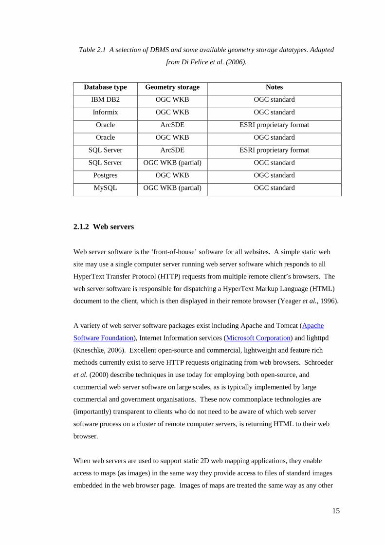
Table 2.1 details the main commercial and open-source DBMS systems in use today, along
with the most prevalent geometry storage types used. Of note, the OGC’s WKB method of
storing geometries is the only non-proprietary storage format available in most spatially
capable DBMSs.
15
Table 2.1 A selection of DBMS and some available geometry storage datatypes. Adapted
from Di Felice et al. (2006).
Database type Geometry storage Notes
IBM DB2 OGC WKB OGC standard
Informix OGC WKB OGC standard
Oracle ArcSDE ESRI proprietary format
Oracle OGC WKB OGC standard
SQL Server ArcSDE ESRI proprietary format
SQL Server OGC WKB (partial) OGC standard
Postgres OGC WKB OGC standard
MySQL OGC WKB (partial) OGC standard
2.1.2 Web servers
Web server software is the ‘front-of-house’ software for all websites. A simple static web
site may use a single computer server running web server software which responds to all
HyperText Transfer Protocol (HTTP) requests from multiple remote client’s browsers. The
web server software is responsible for dispatching a HyperText Markup Language (HTML)
document to the client, which is then displayed in their remote browser (Yeager et al., 1996).
A variety of web server software packages exist including Apache and Tomcat (Apache
Software Foundation), Internet Information services (Microsoft Corporation) and lighttpd
(Kneschke, 2006). Excellent open-source and commercial, lightweight and feature rich
methods currently exist to serve HTTP requests originating from web browsers. Schroeder
et al. (2000) describe techniques in use today for employing both open-source, and
commercial web server software on large scales, as is typically implemented by large
commercial and government organisations. These now commonplace technologies are
(importantly) transparent to clients who do not need to be aware of which web server
software process on a cluster of remote computer servers, is returning HTML to their web
browser.
When web servers are used to support static 2D web mapping applications, they enable
access to maps (as images) in the same way they provide access to files of standard images
embedded in the web browser page. Images of maps are treated the same way as any other

16
online image and returned to the client browser for display (Mitchell, 2005). For 2D
dynamic web mapping however, which is the vast majority of modern-day web mapping
applications, the more advanced features of web server software are exploited.
The Common Gateway Interface (CGI) abilities and server-side scripting of web server
software packages are utilised to create a map (a view of spatial data), ‘on the fly’. Web
server software is able to execute scripts and programs (via the operating system and CGI),
or execute a script itself, making the generation of dynamic maps possible (Yeager et al.,
1996).
For example, a CGI web mapping program such as MapServer (http://mapserver.org/) is able
to access spatial data stored as images, point and lines in proprietary GIS format files or
geometries in a database. The spatial extents, layers and symbology used when creating the
new map can be based on user requirements sent from the user’s web browser. An image
file containing the map is written to a publicly accessible directory on the web server by the
MapServer application. A Universal Resource Locator (URL) to this image (of a map) is
returned to user’s web browser by the web server software, allowing the image file to be
downloaded and displayed by the web browser.
2.1.3 Map and Geo servers
Websites using a commercial or open-source DBMS to store geometries and attribute data of
geographic objects in a database in conjunction with off-the-shelf web server software, must
augment these mature technologies in order to serve spatial data. Web services are described
by Cerami (2002) as “any service that is available over the Internet, using a standardised
XML messaging system, and is not tied to any one operating system or programming
language”.
Map / Geo servers make use of protocols and methods detailed in open-source standards
defined by the OGC, to provide spatial data and mapping capabilities to web sites, using
XML messaging. The OGC maintains the specifications for Web Map Service (WMS), Web
Feature Service (WFS), Web Coverage Service (WCS) and a collection of supporting
protocols. These protocols define the interoperability of server processes enabling access to
spatial datasets, and client processes which seek to interrogate these datasets.

17
Commercial GIS companies also provide their own software and techniques to undertake
web-based mapping of spatial data stored in databases, using proprietary or open-source
geometry types. ArcIMS (Arc Internet Map Server) from ESRI and GeoMedia WebMap
from Intergraph are two commonly used commercial packages. Both of these large packages
provide access to:
• spatial data and maps, via proprietary methods from proprietary desktop GIS
• spatial data and maps, via open-source WMS and WFS standards
• web mapping, via from web browsers.
Whilst the use of spatial data sharing standards such as WMS and WFS should ideally make
the choice of client and server software used for web-based mapping irrelevant, and the
choice of commercial or open-source software academic, this is not the case.
Vanmeulebrouk et al. (2009) report of problems faced when attempting to use OGC WMS
and WFS standards for spatial data interchange. These include version proliferation, lack of
authentication mechanisms, and ad hoc support by software writers for components of the
standards. Interestingly, Najar et al. (2004) described these standards as short term
solutions, shortly after they were released in 2000 and 2002.
Many organisations implement WFS and WMS as an easy method to provide Internet or
Intranet access to corporate spatial data warehouses. Geoscience Australia (2009) provides
almost 200 spatial datasets as WMS layers from its publicaly accessible website. The United
States Geological Service (USGS) and National Oceanic and Atmospheric Administrations
(NOAA) Geographical data Centre (NGDC) each provide public access to over 50 WMS
layers. Of note, most publicly accessible websites advertising WMS make potential users
aware of possible access speed limitations when linking to more than a few layers, especially
when the remote datasets are extensive.
The slow speed experienced by many users accessing some WMS and WFS capable sites is a
constant comment in much of the available literature at this time. The very new Web Map
Tiling Standard (WMTS - OGC future standard) hopes to overcome some of the the speed
limitations of WMS by providing efficient tiling mechanisms for map images on the Map /
Geo server (Bacharach 2009).
The relative immaturity of these standards and the availability of ever increasing network
bandwidth makes their current use somewhat experimental. It is relatively easy to install
18
commercial or open-source software which, once configured, can provide access to spatial
datasets via WFS and access to maps (as image files) of spatial datasets via WMS. Network
bandwidth, client software and the intended purpose of the mapping application however,
will dictate whether access to spatial data via these methods is a reliable solution.
2.2 Mainstream methodologies
There are many methods available today which enable the publishing of spatial data via
standard protocols using the web (Mitchell, 2005). Large commercial interests and the
general public’s wide acceptance of web mapping have resulted in a great amount of effort
being spent in developing technologies. There are extensive scientific and government
applications making use of current and emerging techniques. Elissalde (2007) describes
European Government’s embracing of open-source technologies to achieve their web
mapping requirements.
The various methods for producing a map viewable on a client computer based on spatial
datasets stored on a remote server computer, generally fall into one of two paradigms. Maps
of spatial data are produced either on the server, or on the client. These two paradigms are
described separately in following sections.
Both paradigms can allow the user to interact with the map on the client computer (pan,
zoom etc.), and to control parameters relating to map generation (e.g. layers, projection,
spatial extents). Both paradigms have advantages and disadvantages. Depending on the
target audience, the required functionality, and the desired speed of generation, one paradigm
may be more suitable than the other. Reader (2009) describes the potential for the general
GIS industry to expand greatly at the ‘low-end’ of the market, with the rise of simple map
serving applications via graphical interfaces of spatial data stored in geo-databases.
This implies an expansion of web mapping using server-side mapping, as opposed to using
desktop GIS, which enables the production of maps on a client computer. Examples include
simple maps embedded in mobile phone applications and mapping applications designed to
be very easy to use via a web kiosk.
There are currently many web mapping technologies, which seemingly achieve very similar
goals. The many open-source and commercial, client and server, web and multi-user

19
mapping techniques and their plethora of acronyms can be confusing. Readers are referred
to diagrams in the following sections to assist in clarification of current trends, where
required.
The generic descriptions of client-side and server-side mapping techniques in the next
sections are followed by descriptions of modern web mapping and data visualisation
techniques. Virtual Globes and specialised 3D and 4D data visualisation software are newer
techniques for mapping and visualising spatio-temporal datasets. These techniques can offer
many advantages over traditional planimetric web mapping techniques, overcoming
limitations of support for elevation values and time for example. Whilst neither technique is
web-based or designed to be multi-user, and both require software other than just a web
browser on a client computer, the unique abilities of both techniques are of relevance to this
research.
20
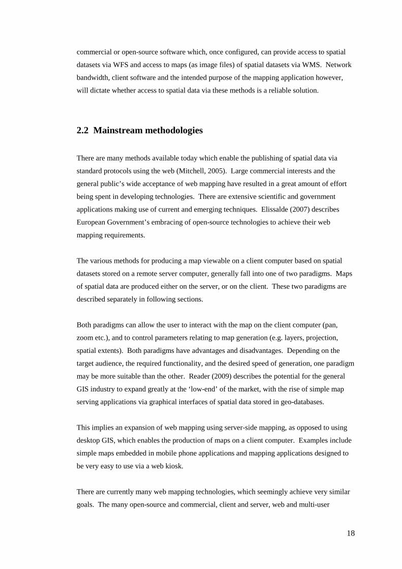
2.2.1 Server-side map generation
Server-side web mapping is a technique which generates a map (as an image) via software
running on a remote web server. A copy, or URL to the image file, representing a map, is
returned to the client computer. This can be undertaken using either proprietary or open-
source Map / Geo server software. OGC WMS standards can be used to specify the map’s
spatial extents or the desired layers for instance. Non-OGC techniques can also be used,
based on client-side HTML form variables and server-side scripting, as has been available
with MapServer (originally from the University of Minnesota) for many years (Kropla,
2005). Figure 2.1 shows an overview diagram of an example OGC WMS implementation of
server-side simple web mapping.
Server-side web mapping generally places the least overhead on the client computer, and the
communication link between the client computer and the remote data sources. The client
computer may need nothing more than web browser software, required plug-ins such as
JavaScript, and a connection to the Internet. As outlined previously, a website can be easily
built which allows very good interaction with the map via a range of useful tools for
navigation and queries.
Figure 2.1 Overview of OGC WMS method of server-side mapping.

21
A variety of Australian Federal and state Government agencies such as the Australian
Capital Territory (ACT) and Tasmanian Governments, Geoscience Australia (GA) and
Australian Natural Resources Atlas (DEWHA) maintain mapping websites utilising server-
side mapping.
Figure 2.2 shows a simple implementation of an open-source map server package
(MapServer), in conjunction with a web server, for the creation of a server-side web
mapping website. In this case, HTML is returned to client’s web browsers, which contain
embedded URLs to image files (of maps) stored in publicly accessible directories on the web
server.
Figure 2.2 Overview of a server-side web mapping system, using MapServer
open-source software (originally from the University of Minnesota)
As the client computer does not require direct access to the spatial datasets, data providers
can place data sources behind corporate firewalls, or implement security or data
generalisation techniques as required. Tight control can be maintained over access to spatial
datasets where this is a requirement, preventing multiple copies proliferating throughout an
organisation’s Intranet or downloaded datasets being used for inappropriate purposes.

22
Google Maps and Yahoo Maps are the currently best known examples of web-based server-
side mapping technologies. Their influence on desktop and mobile mapping is great and a
large number of people who would otherwise not be familiar with web mapping have
become very familiar with Google Maps.
The use of standards such as HTTP, HTML and JavaScript for use in providing web
mapping is commonplace. Whilst these mature and evolving technologies were not designed
with web mapping applications in mind, they currently support a vast array of web mapping
applications. Many web sites providing spatial exploration and mapping services based on
these mature technologies offer excellent functionality, such as panning, zooming and
feature selections, for instance.
There can be a large number of options available when choosing the DBMS, web server
software, Map /Geo server software, client and server-side languages, and file format(s) to
use when building a new website. There is a divide between those methods using
proprietary commercial software from large commercial GIS software companies and those
methods employing wholly open-source techniques (Elissalde, 2007). It is often difficult to
integrate a custom requirement into proprietary techniques due to a lack of documentation of
protocols, for example.
Whilst desktop GIS from ESRI, MapInfo (Pitney Bowes), Autodesk and other commercial
providers support spatial data with elevation values, enabling 3D views via desktop GIS
software, no vendors offer tools for server-side web-based 3D or 4D data visualisation.
Open-source GIS software, and open-source Map / Geo server software such as UMN
MapServer and GeoServer are also unable to support elevation in spatial datasets. Maps
produced via these techniques are limited to planimetric views and oblique views are not
currently possible.
Virtual Globe browsers (such as Google Earth or NASA Worldwind) do not suffer from this
limitation. Google Earth is a hybrid technique for interactively viewing spatial data in a 3D
environment. It can be described as a hybrid technique as background imagery and vector
layers are streamed via proprietary methods from remote Google servers, but there is the
provision for the generation and fine control of spatial datasets on the user’s computer.
Elvidge et al. (2008) discusses the burden of spatial data management “lifted from the
shoulders” of those who use Google Earth’s imagery for research purposes. Rather than
attempting to purchase and maintain their own library of remote-sensed images, researchers

23
are able to utilise Google Earth imagery. Virtual Globe browsers are described in a later
section of this chapter.
2.2.2 Client-side map generation
Client-side web mapping implies spatial data is sent from the remote server to the client
computer, where a map is generated locally (Mitchell, 2005). The data can be transferred via
proprietary protocols, or via open-source OGC standards such as WFS. The OGC WFS
methodology importantly allows the download of spatial data to a client, as opposed to the
download of a map (image) of spatial data. Symbology is applied on the client computer,
allowing customisation as required by the user. Data can be saved locally and used in GIS
operations. The WFS protocol also supports the editing of remote datasets when compliant
client software is used with compliant server software.
The generation of maps on a client’s computer using specialised software, can be
advantageous in many respects. Limitations of current web browser technologies can be
removed when client software designed exclusively to allow the access and display of spatial
data is used. This can be advantageous for many Intranet applications where the abilities and
requirements of users exceed that of the general public.
The use of specialised software and the need to provide access to raw spatial datasets can
come at a cost. The steep learning curve for using some mapping and GIS software, and the
resulting barrier this can often cause is described by Donald (2005). The overlap of
functionality between a full featured GIS and a lightweight desktop mapping application can
cause confusion amongst those unfamiliar with GIS and mapping technology. The need to
transfer highly detailed spatial data when undertaking broad scale client-side mapping,
instead of transferring a simple raster image, can be bandwidth prohibitive.
Steiniger et al. (2008) provide a comprehensive list of available open-source full featured
desktop GIS software. The list includes software which could be used to replace a
commercial desktop GIS, provide a lightweight client mapping utility, or software which
could fill either role. An overview of open-source and free lightweight desktop software for
connecting to remote servers offering WMS and WFS is maintained by National Aerospace
Laboratories Netherlands (NLR) on their website (Geospatial Dataservice Centre, 2009).
24
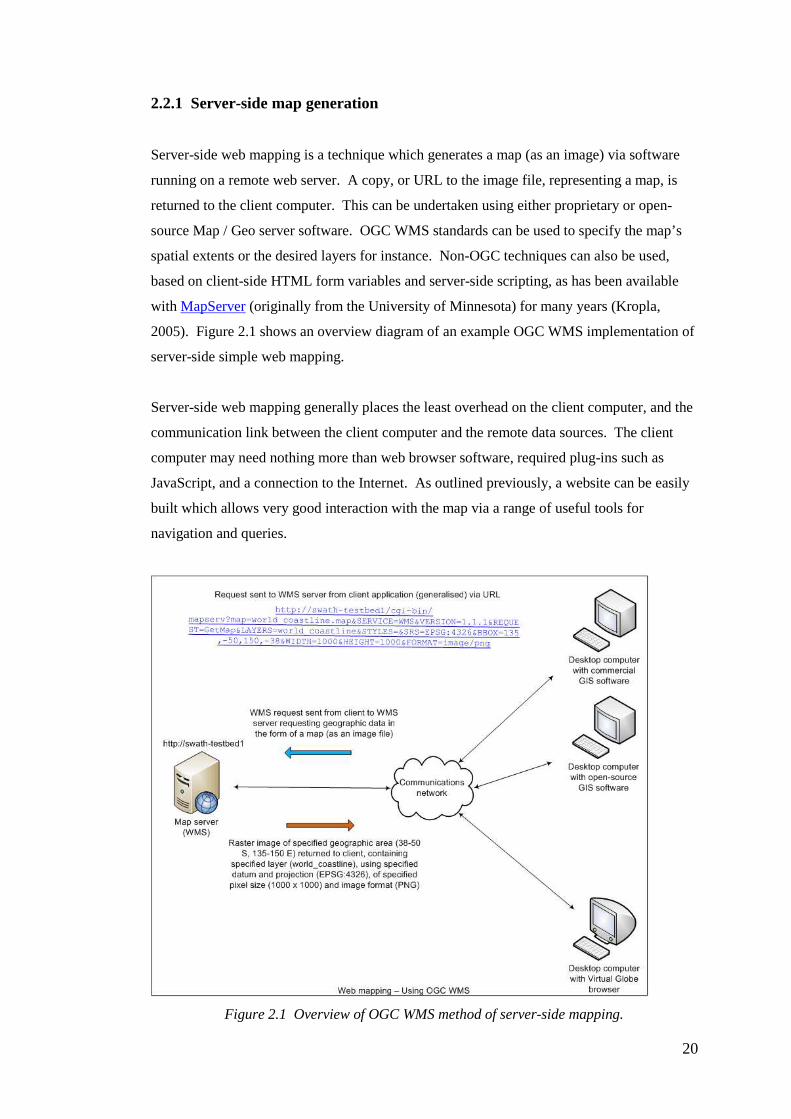
Figure 2.3 Overview of OGC WFS method for client-side mapping.
The ability to serve spatial data via the web with elevation values and ancillary data was
realised with the development of Keyhole Markup Language (KML) in 2001 (Wernecke,
2009). KML is an Extensible Markup Language (XML) based data-interchange format that
allows the description of geographic objects, and ancillary data used when visualising the
objects, via a KML capable browser (Wilson, 2007).
KML provides a method to encapsulate the geometry of points, lines and polygons
(representing real-world objects or phenomena), geocoded raster imagery, metadata,
symbology, and view point parameters in one file. A compressed file (KMZ) can be served
via standard web protocols such as HTTP or FTP, or accessed via a fileshare from a remote
or local file system. KML has been accepted by the OGC as an open standard (2008) and
continues to develop. KML version 2.2 is the current release.
Geo / Map server applications such as GeoServer have been created to serve KML files to
clients, based on local (to the server) spatial data stored via a range of mechanisms
(GeoServer, 2009). KML’s support for both the elevation and temporal components of
spatial datasets enables both the modelling of real-world phenomena and the exploration of
models via Virtual Globes.
25
2.3 Virtual Globes
The release of KML in 2005 coincided with the release of the Google Earth application by
Google Inc. Google Earth, NASA Worldwind, ESRI ArcExplorer and some less fully-
featured software packages allow the graphical presentation of spatial data in an intuitive 3D
globe view. 3D Virtual Globes can be manipulated on the 2D computer screen with a
mouse, much the same as a traditional floor standing world globe can be spun by hand.
Layers can be added or created, and turned on or off, to suit user needs.
Discussions of Google Earth functionality are often focused on the quality of the freely
available remote sensed imagery supplied by Google servers to Google Earth Virtual Globes,
rather than the browser’s abilities. For this thesis, the capabilities and limitations of the
Google Earth Virtual Globe browser are of most interest, rather than the Google supplied
imagery.
A Virtual Globe browser can enable the creation of intuitive 3D views of spatial data on a
client computer, using both local and remote datasets. Most current Virtual Globe browsers
support access to spatial datasets via standards such as KML, WFS and WMS. Dunne et al.
(2006) describe the use of Google Earth and KML for visualising marine datasets around
Ireland. Dunne remarks the combination of a Virtual Globe browser such as Google Earth
with OGC standards such as KML and WMS, makes the web-based exploration of large
multi-beam echo-sounder imagery possible.
Of note for research undertaken in completing this thesis, Dunne also concludes a major
limiting factor of using Google Earth (in 2006) for marine studies is its lack of a digital
elevation model for the ocean. Blower et al. (2006) likewise makes note of this limitation in
Google Earth when describing the features of a Google Earth, KML and WMS based system
for marine data exploration. This limitation was removed with the release of Google Ocean
in 2009. Google Earth (version 5 and above) now provides worldwide coverage of both land
elevations and ocean depth values.
It is not currently possible to replace the Google supplied undersea terrain model with a
higher spatial resolution Digital Elevation Model (DEM). This is a limitation for some
scientific applications, although techniques such as overlaying high spatial resolution
illuminated bathymetric colour images over the monochromatic Google DEM can give an
excellent illusion of a higher spatial resolution DEM. This technique suits many applications
26
where an illuminated high spatial resolution DEM derived from Multi-Beam Echo-Sounders
(MBES) is available, for example.
A major advantage of using Google Earth in conjunction with KML for firstly distributing,
and secondly visualising, spatial datasets is the simplicity of the technique. An almost
endless number of vector and raster layers, containing annotation and symbology can be
encapsulated into a single compressed KML file (KMZ format). This single compressed
binary file is easily emailed to a user who has Google Earth installed. On opening, the
vector and raster layers within the KMZ file will appear on the new user’s Virtual Globe,
alongside any existing datasets they have. The annotation and symbology applied by the
creator of the KMZ file will appear on the new user’s Virtual Globe with the same colours
and fonts as originally specified.
Google Earth supports the <network link> method in the KML language which enables the
automatic periodic re-loading of a remote dataset. This can remove the need to send large
static KML or KMZ files to multiple users. A small KML format file containing a link(s) to
large and possibly dynamically generated KML or KMZ file can be sent to interested
persons, without the risk of proliferating large out-of-date spatial datasets. Complex and
dynamic up-to-date views of real-time processes can be created by this centralised technique.
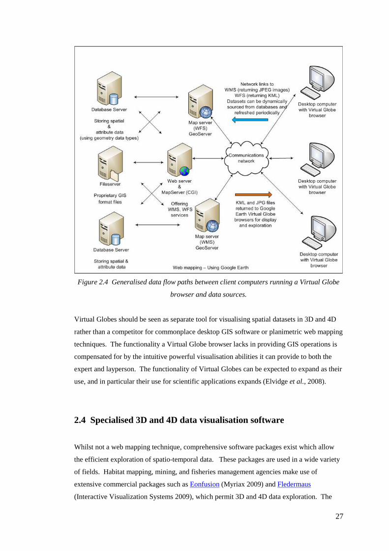
Figure 2.4 shows an example of the types of data sources which could be used to supply
dynamic spatio-temporal data to multiple Google Earth clients. The excellent connectivity
abilities of most Map / Geo server applications such as GeoServer, and web server CGI
based applications such as MapServer, allow for complex spatial data source configurations
if required as shown.
A criticism of Virtual Globe technology is the lack of control experienced users may
perceive. Desktop GIS software users are used to being able to apply datum shifts as
required, display the mouse pointer units in projected or unprojected units, and exactly
control the scale of on-screen or printed maps. No Virtual Globe browsers currently
available support all of these standard GIS software functions. Whether this is a valid
criticism is debatable. By necessity, most commercial desktop GIS software packages are
powerful full-featured systems, providing a wide range of tools to suit a wide range of users.
GIS software can, however, appear overly complicated and daunting for new or infrequent
users, even when attempting to create a simple map (Hatcher et al., 1999).
27
Figure 2.4 Generalised data flow paths between client computers running a Virtual Globe
browser and data sources.
Virtual Globes should be seen as separate tool for visualising spatial datasets in 3D and 4D
rather than a competitor for commonplace desktop GIS software or planimetric web mapping
techniques. The functionality a Virtual Globe browser lacks in providing GIS operations is
compensated for by the intuitive powerful visualisation abilities it can provide to both the
expert and layperson. The functionality of Virtual Globes can be expected to expand as their
use, and in particular their use for scientific applications expands (Elvidge et al., 2008).
2.4 Specialised 3D and 4D data visualisation software
Whilst not a web mapping technique, comprehensive software packages exist which allow
the efficient exploration of spatio-temporal data. These packages are used in a wide variety
of fields. Habitat mapping, mining, and fisheries management agencies make use of
extensive commercial packages such as Eonfusion (Myriax 2009) and Fledermaus
(Interactive Visualization Systems 2009), which permit 3D and 4D data exploration. The

28
availability of fast and affordable desktop computers, with powerful graphics capabilities,
has made the use of these powerful desktop packages possible.
Improvements in technology, in particular scientific data acquisition and logging
technologies, has increased sample rates and data volumes of spatio-temporal data beyond
the limits of currently available mapping and GIS software. General mapping and GIS
software is unable to effectively accommodate either the volumes or the time component of
large spatio-temporal datasets. Malzone et al. (2009) describe the effect of these limitations
as leaving only a “best guess” approach. Limitations are most evident when combining and
visualising complex 4D datasets with general purpose mapping and GIS software, and
looking for answers to complex interactions.
Commercial software packages such as Eonfusion and Fledermaus offer a variety of
licensing options. These options affect not only the type of license (single user or floating,
for instance), but also the software functionality. For instance, to support real-time data
within Fledermaus, the professional version of the package must be purchased. The data
sources that can be used with these packages include databases, ESRI shapefiles, text files
and realtime serial data from a navigation source.
Whilst these packages are powerful, and can meet a wide variety of needs, they can be
daunting for first-time users and they are not intended to be used as generic multi-user
mapping tools. As well as being faced with a steep learning curve, users are faced with a
substantial financial outlay. A single seat, base version of Fledermaus Pro costs over $10
000 AUD (August 2009), depending on discounting. In many circumstances the purchase
cost is justifiable as there are currently few other methods to visualise 4D datasets.

29
Chapter 3 Methods
This chapter describes the methodology used to assess the abilities of a spatio-temporal
DBMS combined with KML. The assessment of these abilities was in the context of
fulfilling a need to provide real-time multi-user capabilities, when exploring spatio-temporal
datasets during a marine research voyage. The results of this assessment are detailed in
Chapter Four.
Datasets collected routinely and automatically by research vessel’s data acquisition systems
are collected versus position and time. A research vessel is a moving platform and the 3D
position a measurement is made at, is as important as the time it is taken. Measurements and
observations on a typical modern research vessel are taken by a wide range of instruments
which can be mounted on, towed behind, lowered from or tethered to the vessel.
Measurements of the same physical phenomena taken at different locations at the same time
are common, such as Photosynthetic Active Radiation (PAR) measurements from a vessel
mounted sensor and a sensor fitted to a vertically lowered instrument.
Ideally, the 3D path a Remotely Operated Vehicle (ROV) takes above the seabed beneath a
research vessel should be able to be easily visualised with the path a towed video camera
sled took the day before, or the voyage before. Water chemistry parameters measured in 4D
by the ROV, such as turbidity or pH, should be able to be visualised in 4D, along with the
3D positions of features of interest identified in imagery captured by the video sled.
A real-time method allowing the efficient collation, storage and exploration of 4D real-time
datasets during a research voyage, could confirm the operating performance of equipment
and give confidence in survey design. Linkages between the co-located datasets generated
by these two instruments should be made in real or near real-time whilst the research vessel
is in the study region. However, typically the 4D spatio-temporal datasets from the
underwater instruments above would be recovered from the in-house developed or vendor
supplied equipment data acquisition and control computers, after the instruments are
recovered. Differences in the formats of the datasets which may prevent direct comparison,
such as differing co-ordinate systems, vertical datums, data logging rates or time references
would need to be resolved. The datasets would then be imported into a commercial desktop
GIS or a 3D or 4D data visualisation package and attributes versus 3D space and time could
be visualised or mapped.

30
The process described above, requires access to specialised software and knowledge before a
simple single-user visual analysis process can be undertaken. Due to limited berths on most
research vessels, financial constraints and time pressures, the data importation, collation and
visual analysis steps described may not be undertaken until the vessel returns to port, or has
left the survey area. Instrumentation problems such as fouled sensors, or the lack of
underwater lighting to resolve the source of a spike in pH or turbidity readings, once
discovered after leaving the survey area, cannot be resolved. Problems which affect ROV
performance, such as attitude (pitch / roll) bias due to water pressure, which are found when
visualising recorded datasets ashore such as ROV operating parameters versus depth and
time, cannot be retrospectively corrected.
There is a need to provide easy access to all spatio-temporal data routinely collected on
research vessels such as underway data (tied to a vessel’s location), waypoint lists (both past
and future) and the paths of deployed instruments. As previously described, the collection of
in-house developed and vendor supplied software packages used on the majority of research
vessels do generally allow the very reliable digital logging of all parameters of interest
versus time and / or location. However, no technique currently exists that enables the
creation of a holistic real-time 4D view of spatio-temporal data collected by these (often)
disparate data acquisition systems.
As part of this research, a server-based system was constructed for use at sea, allowing the
4D visualisation and exploration of real-time and historic spatio-temporal datasets. Hatcher
et al. (1999) describe the use of client-server methodology for supporting multiple users at
sea on research voyages. Hatcher et al. make note of the necessity to make this a feature at
the start of the design process, for a vessel-based, data acquisition and distribution system.
The name chosen for the software tool developed in this study was MARVIN – MArine Real-
time VIsualisation Network. MARVIN encompasses the computer server, server-side
programs and the DBMS.
This chapter does not attempt to exhaustively describe the full functionalities of every
software package used nor the intricacies of generally well known protocols and standards.
By design, most of the software components used in testing the hypothesis of this thesis are
well documented and mature products. Where an explanation has been deficient, interested
readers are referred to the documentation readily available for all of the software components
used.

31
However, the unique capabilities provided by the combination of these commonly available
software components, does deserve detailed explanation. Explanation is provided in the
remainder of this chapter. The following sections describe: the hardware and software
components, and the test datasets used in building MARVIN. The remainder of the chapter
is devoted to describing in detail the processes and data paths within MARVIN, based on the
software chosen and the specialised programs written. Where appropriate, block diagrams
have been included to augment descriptions of the various datasets, processes, data paths and
protocols.

32
3.1 Introduction
The primary factors determining the selection of the software and datasets used to undertake
this research are as follows:
• MARVIN must accommodate spatial data containing both positive and negative
(depth) elevation values.
• MARVIN must accommodate time, allowing the interrogation, exploration and
visualisation of spatial data in both time and space.
• MARVIN must support multiple concurrent users, providing access to all features
via Virtual Globe browsers, allowing centralised real-time spatio-temporal datasets
to be integrated into each user’s browser and combined with any specific spatial
datasets as required.
• The datasets chosen to test MARVIN must be typical of those collected at sea on
modern research vessels during marine science voyages.
All software packages used for the creation of MARVIN are ideally open-source, using
standards and protocols which were well documented and non-proprietary. This philosophy
can allow the creation of systems such as MARVIN which are not based around specific
vendor protocols or versions of proprietary software. This is a philosophy which can be
adopted when building systems for scientific or research use, where the limiting constraint is
often financial, rather than time or expertise.
The various components of MARVIN are best described separately before detailing how the
system worked as a whole. The following sections describe the hardware, software and
datasets used.

33
3.2 Hardware
3.2.1 Server computer specifications
A single Intel based personal computer was used for all server-side tasks. For scalability or
security reasons, it would have been feasible to run the DBMS, HTTP server and server-side
scripting processes on multiple computers. For simplicity and physical portability, a single
personal computer was utilised. Table 3.1 lists the modest specifications of the computer
server.
Of note is the use of a personal computer with a single physical hard disc drive, supporting
the operating system, DBMS and web server root directory. This is a very simple
implementation for a multi-user, database intensive application such as MARVIN. Whilst
the resulting server hardware proved functional, the performance limitations of this simple
approach should be appreciated.
Table 3.1 Relevant hardware specification of computer server.
Manufacturer Hewlett Packard
Processor Intel Core 2 Duo 1.86 GHz
Memory and memory speed 4 GB / 833 MHz
Hard disk 80 GB 7200 RPM Hitachi SATA
Network interface card Intel 82566 integrated Gigabit
Operating System Linux - Fedora 8 (2.6.26.8-57)

34
3.2.2 Client computer specifications
Three separate computers with Google Earth installed were utilised for test purposes. A
variety of Operating Systems (OS), Central Processing Unit (CPU) speeds and video card
capabilities are represented in the computers used. The capabilities of the computers used
were typical of mid priced computers used by Government and research organisations that
have an Information Technology purchasing arrangement with a large computer supplier.
Table 3.2 details relevant specifications of each machine.
Table 3.2 Relevant specifications of the three client computers used to run Google Earth.
Manufacturer DELL DELL DELL
Model
Precision
T5400
Optiplex
745
Latitude
520 laptop
Processor Intel Xeon 2.5
GHz quad core
Intel Duo 3.6
Ghz dual core
Intel T2300
1.6 Ghz
Memory 4GB
833 MHz
4GB
533 MHz
500MB
667MHz
Hard disk 500GB 10k RPM
SAS
80GB 6.5k RPM
SATA
40GB 5.4k RPM
PATA
Network interface
card
Broadcomm
Gigabit
Intel integrated
Gigabit
Intel integrated
Gigabit
Operating System Windows XP Pro
64 bit 2003.
Windows XP Pro
32 bit SP2
Windows XP Pro
32 bit SP3

35
3.3 Software
As previously mentioned, a major factor determining the choice of all software components
used in creating MARVIN was the availability of documentation and relevant examples.
Capabilities of the software components used in supporting this research are described in this
section.
3.3.1 DBMS – PostgreSQL / PostGIS
PostgreSQL 8.2.11 (03/11/2008) was selected as the DBMS for use with MARVIN
(http://www.postgresql.org). The ability to store OGC compliant geometries was added via
the PostGIS extensions 1.3.5.1 (15/12/2008) (http://postgis.refractions.net ). PostgreSQL /
PostGIS was chosen as the DBMS due to the package’s mature support for OGC compliant
geometries and the large community which currently uses the PostGIS extension. ESRI have
recently supported the native connection of their desktop GIS application (ArcMap v9.3) to
PostGIS for the storage of spatial datasets, alongside commercial DBMSs with mature
spatial data support such as Oracle Spatial and IBM Informix DataBlade. This is as an
indication of the commercial GIS industry’s confidence in PostGIS for spatial data storage.
The very popular open-source MySQL DBMS could also have been used. It is the preferred
open-source DBMS for many web-based applications, supported by many Internet Service
Providers (ISP). The relative immaturity of MySQL’s support for advanced database
functions such as views (virtual tables), OGC OpenGIS Simple Features Specifications For
SQL (Open Geospatial Consortium Inc., 2005) and OGC geometries negated the advantages
of using this very popular DBMS for this research. Its use in supporting similar research
topics in the future should be reconsidered as its spatial data handling capabilities mature.
3.3.2 Web server – Apache HTTP
Apache HTTP server 2.2.9-1 (12/06/2008) was selected to serve HTTP requests from client
computers running Virtual Globe browsers accessing MARVIN (http://www.apache.org).
Apache HTTP server was installed as part of the OS for the server computer and it is a
widely used open-source web server software package. Apache is included as part of the
commonly available LAMP (Linux, Apache, MySQL and PHP / Perl / Python) open-source

36
distribution package and therefore has a large install base. Its large install base and maturity
has resulted in the availability of excellent documentation.
Other web server packages such as Lighttp (Kneschke 2006) or AOLserver could have been
used, possibly with some speed advantages due to their reported scalability. No security
functions (HTTPS), multi-scaling or advanced functionality was required for this research.
3.3.3 Server-side scripting languages
PHP
PHP (PHP Hypertext Processing) 5.2.6 (02/05/2008) provided server-side scripting
capabilities (http://www.php.net). Server-side scripts were used to dynamically generate
KML datastreams which were returned by the web server to the client’s Virtual Globe
browser for interpretation and display.
PHP’s integration with Apache, the availability of the pgsql module (v8.2.7) permitting
connection to PostgreSQL, and the availability of the JpGraph package (see below) for
dynamic raster chart generation, were reasons for the language’s choice for supporting this
research.
Other programming languages which could have been used for server-side programming
include Perl and Python. The Python programming language possesses excellent database
connectivity and there a variety of scientific graphing packages available. Indeed, any
language capable of being executed by the server computer operating system could have
been utilised by using Apache’s support for common gateway interface (CGI) programs.
CGI allows programs to be executed on a web server computer via a HTTP request from a
remote client. CGI programs can interact with local or remote DBMSs as required, before
returning HTML (or in this case KML) to the client’s browser.
This is in contrast to the philosophy of PHP programs which are executed by the web server
application (Apache in this case) rather than by any external process, such as a Python shell
or Java’s Runtime Engine (JRE). The coupling of the server-side language (PHP) to the web
server application removed the requirement for the installation of any shells, engines, or
interpreters on the web server for KML generation, simplifying the configuration of the web
server software.
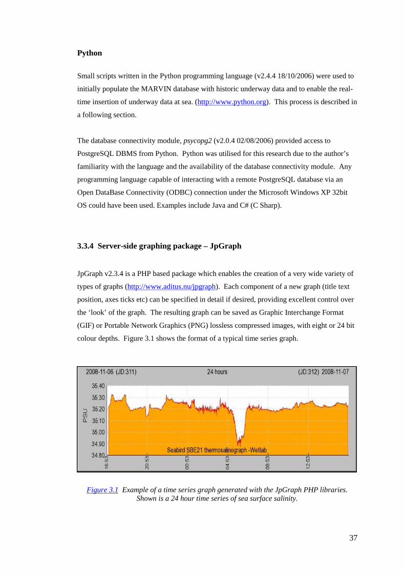
37
Python
Small scripts written in the Python programming language (v2.4.4 18/10/2006) were used to
initially populate the MARVIN database with historic underway data and to enable the real-
time insertion of underway data at sea. (http://www.python.org). This process is described in
a following section.
The database connectivity module, psycopg2 (v2.0.4 02/08/2006) provided access to
PostgreSQL DBMS from Python. Python was utilised for this research due to the author’s
familiarity with the language and the availability of the database connectivity module. Any
programming language capable of interacting with a remote PostgreSQL database via an
Open DataBase Connectivity (ODBC) connection under the Microsoft Windows XP 32bit
OS could have been used. Examples include Java and C# (C Sharp).
3.3.4 Server-side graphing package – JpGraph
JpGraph v2.3.4 is a PHP based package which enables the creation of a very wide variety of
types of graphs (http://www.aditus.nu/jpgraph). Each component of a new graph (title text
position, axes ticks etc) can be specified in detail if desired, providing excellent control over
the ‘look’ of the graph. The resulting graph can be saved as Graphic Interchange Format
(GIF) or Portable Network Graphics (PNG) lossless compressed images, with eight or 24 bit
colour depths. Figure 3.1 shows the format of a typical time series graph.
Figure 3.1 Example of a time series graph generated with the JpGraph PHP libraries. Shown is a 24 hour time series of sea surface salinity.

38
Importantly, JpGraph supports the concept of null values. This was necessary when creating
a time series graph of an underway parameter within MARVIN and for various reasons one
or more ten second interval datapoints were missing. The resulting graph was able to
‘honour’ the missing value(s) by including a discontinuity in the line plot and filled area at
the position of the missing point(s). This is important when the time-series graphs are used
as a quality control tool for fault-finding missing datapoints in one or more underway
parameter datasets.
Some competing open-source graphing packages are unable to accommodate missing values
in time series graphs and join datapoints on either side of missing points by a continuous
line. ‘Null’ values such as zero, a large positive or a large negative value must be
programmatically assigned to missing values to enable the creation of time series graphs
which support discontinuities, when using these competing packages. Whilst often adopted
to overcome graphing limitations, this method can erroneously mask missing datapoints if
the process is not undertaken correctly.
JpGraph was utilised within this research to generate time series graphs of underway data
parameters such as sea surface temperature or barometric pressure. PNG images of graphs
written to publicly accessible public directories on the server computer, were referenced in
the KML datastream parsed by the Virtual Globe browser on the user’s computer. The
images (of graphs) were subsequently downloaded as required by the Virtual Globe browser.
3.3.5 Server-side mapserver package – MapServer
The MapServer v4.10.3 package in conjunction with the PHP Mapscript option (04/04/2007)
was utilised for the server-side creation of planimetric maps for use in MARVIN
(http://mapserver.org). MapServer can be used as a CGI program, installed as a single
executable file with associated libraries, or its functionality can also be accessed through the
use of a MapScript module for the language of choice. The PHP Mapscript module was used
for all 2D planimetric mapping in MARVIN. MapServer CGI was used for test purposes for
making spatio-temporal data in MARVIN’s database available to desktop GIS clients via
OGC WMS for functionality assessment (as discussed in Chapter Five).
MapServer was chosen for its stability and maturity, the availability of many excellent on-
line tutorials, and its integration with PHP. MapServer has a large install base and
challenges commercially available map-serving applications. It supports a wide variety of

39
vector and raster geospatial data formats typically used by research organisations such as
ERSI shapefiles and GeoTIFFs. Importantly for this research, MapServer is able to access
OGC compliant geometries stored in a PostgreSQL database.
3.3.6 Virtual Globe browser – Google Earth
The Virtual Globe browser used was Google Earth v5.0 (http://earth.google.com). Google
Earth is free for personal use but is not open-source. The software used to present a Virtual
Globe to the user and allow interactive panning, zooming and selection may be the only
piece of software a user associates with a real-time data visualisation system. The elegance
of the database design, the clarity of the time series graphs or the general capabilities of the
system may be dismissed by a new user if he or she is dissatisfied by the Virtual Globe
browser.
The competition between open-source and commercially available web browsers over the
last 15 years has resulted in the availability of many excellent and stable web browsers such
as Mozilla Firefox, Opera and Internet Explorer. The competition between Virtual Globe
browsers has only existed for the last five years and as such, standards and capabilities are
still developing. Whilst Google Earth was chosen in support of this research, competing
open-source and commercial products such as NASA World Wind or ArcGIS Explorer were
considered.
A major research requirement for this thesis was to utilise KML for the real-time packaging
of dynamic spatio-temporal data. Therefore, the use of a Virtual Globe browser which
complied with the OGC KML 2.2 Reference – an OGC Best Practice standard was a
requirement (Open Geospatial Consortium Inc., 2007). Of note, the Network Link element
defined in the standard was utilised during this research to permit the automatic refresh of
4D views based on data sourced via dynamic KML datastreams.
Whilst Google Earth and KML have long been associated, the new ownership of the
development of the KML standard by the OGC (April 2008) has broken the link between the
developing Virtual Globe browser and the developing spatial data interchange standard.
Whilst in theory any fully OGC compliant Virtual Globe browser could be used to access the
dynamic KML datasets produced during this research, only Google Earth currently supports
the Network Link element within the KML standard.

40
One option to overcome this current limitation would be to use mechanisms such as WMS or
WFS, rather than KML in conjunction with Network Links, for accessing remote real-time
spatial temporal datasets. Likewise, the need to install a stand alone application such as
Google Earth on every computer accessing MARVIN could be overcome. By using a
ubiquitous web browser with the required plug-in for the Google Earth Application
programming Interface (API) or Microsoft Virtual Earth (Bing maps for Enterprise) API, a
web browser based tool (containing a Virtual Globe) could be developed.
The use of either API in conjunction with a web browser for embedding a light weight
Virtual Globe within an HTML document was discounted for use in this research. The
necessity for the web browser on the client computer to connect to either Google or
Microsoft servers to generate the Virtual Globe cannot currently be seen as a robust solution
for use in a field environment.
Such options do offer advantages however, such as allowing the building of a fully
customisable Graphical User Interface (GUI) within a standard web browser and the removal
of the requirement to install an application such as Google Earth on multiple client
computers. These advantages are applicable when building multiple ‘kiosk’ style embedded
browsers for use on research vessels in various wet laboratories and spaces, for example. A
limited feature software application which utilises Virtual Globe technologies could be used
on a solid state (no moving parts) ruggedised computer with an integrated touch screen
display. This would permit access to a server-based system such as MARVIN, for underway
data display and waypoint entry, from the many ‘computer hostile’ locations on a research
vessel.

41
3.4 Datasets
The spatio-temporal datasets chosen as the basis for this research were either real-world
empirical datasets or simulated datasets. The datasets chosen were typical of those collected
aboard modern blue-water (operating outside of sheltered water) marine research vessels.
These vessels typically utilise commercial or in-house developed data acquisition, display
and dissemination systems, as well as specific vendor supplied applications.
MARVIN is not reliant on data formats specific to individual manufacturer’s equipment.
The individual peculiarities and interfacing requirements of equipment undertaking
measurements are accommodated by the vessel’s main data acquisition system. Once spatio-
temporal data is correctly stored in MARVIN’s database by the main data acquisition
system, data can be visualised in space and time regardless of whether the point represents:
• an empirical measurement of sea surface temperature from ten seconds prior
• a user-entered waypoint to steer to tomorrow
• the 3D path a fishing net took through the water the day before
3.4.1 Real-world collected datasets
The real-world datasets used for testing were sourced from the CSIRO Division of Marine
and Atmospheric Research (CMAR) Divisional Data Centre (DDC). 43 million rows of
underway data collected during 2009 aboard the research vessel Southern Surveyor were
used. This large dataset was imported into the MARVIN PostgreSQL DBMS, sourced from
the DDC’s Oracle DBMS. The dataset contained a variety of measured underway
parameters, such as air temperature and vessel speed, recorded electronically by the vessel’s
data acquisition system during the nine marine science voyages throughout the year.
Values were stored every ten seconds during a typical three week voyage resulting in almost
200 000 readings per voyage, per data type. Table 3.3 details the data types and units of the
13 parameters able to be visualised in MARVIN. The vessel’s latest position, updated every
ten seconds in the DBMS, allowed the vessel model shown in Google Earth to be positioned
correctly in real-time, for example. Likewise, the multitude of underway parameters, such as

42
relative humidity, sea surface temperature or water depth, were able to be visualised in
Google Earth, both in space aligned with vessel track and in time-series graphs.
Table 3.3 Underway dataset parameter details
Description Units Equipment
Atmospheric air pressure mBar / hPa Vaisala electronic barometer
Air temperature degrees C Vaisala electronic thermometer
Course over ground (COG) degrees (true) Seapath 200 GPS system
Depth metres Kongsberg EM300 multi-beam
echo-sounder
Fluorescence (Sea surface) Unitless /
ratiometric
Wetlabs ECO-FLD
Heading degrees (true) Kongsberg Seapath 200 GPS
system
Humidity percent Vaisala electronic thermometer
Photosynthetic active
radiation (downwelling)
µmoles / second /
m2
Licor LI-192SB (300-700nm)
Salinity (Sea surface) PSU Seabird SBE21
thermosalinograph
Speed over Ground (SOG) Knots Seapath 200 GPS system
Temperature (Sea surface) degrees Celsius Seabird SBE21
thermosalinograph
Wind Direction degrees (true) RM Young 05103 anemometer
Wind Speed knots RM Young 05103 anemometer
3.4.2 Simulated datasets
Along with real-world empirical datasets, a number of datasets were simulated to allow the
realistic evaluation of MARVIN, and hence the underlying technologies of interest for this
research. The datasets simulated were typical of those collected on blue-water research
vessels, generally in stand-alone data acquisition systems rather than via a centralised
underway data acquisition system.

43
The geographic position of the data contained within the simulated datasets were not the
same as vessel position, for a given time, unlike the underway datasets which always used
the vessel position as a reference. For example, a net towed behind a vessel during trawling
operations does not exist in the same position, at the same time, as the vessel. Likewise, a
profiling instrument lowered vertically beneath a vessel has a differing depth value, versus
time, to the vessel which remains on the sea surface. This is in contrast to underway datasets
(sea surface temperature, wind direction etc), which are referenced to location of the vessel
as the measuring equipment is physically attached to the vessel.
Multi-Beam Echo-Sounder (MBES) Coverage
Large blue-water research vessels are often fitted with low frequency Multi-Beam Echo-
Sounder equipment (MBES) and associated vessel attitude and position determining systems
for seabed mapping.
This equipment maps a swath of the seabed across the direction of travel of the vessel.
Swath widths can typically be up to six times the water depth, depending on the water depth
and sea state. Hence, a swath width of 6000 metres across the direction of travel may be
realised when working in water depths of one kilometre. This 6000 metre line across the
seabed may be sampled spatially between 100 and 200 times along it length, depending on
the type of MBES installed. This implies an ensonification spacing of 30 to 60 metres on the
seafloor. This in turn dictates the appropriate cell size for any resulting interpolated raster
grids of depth values. Figure 3.2 shows a view of swath coverage, as visualised in
MARVIN. The generation of the image in this figure is discussed in Chapter Four.
Software supplied by the manufacturers of MBES such as Kongsberg (Norway), Reson
(USA) and Klein (USA), and third party software from companies such as QPS
(Netherlands), HYPACK (USA) or EIVA (Denmark) allow the control of the sonar and
creation of bathymetric datasets. Most MBES control / quality control (QC) software
packages allow a variety of 2D and 3D graphs, and surfaces to be generated in real-time for
QC purposes for interpretation by the trained operator. Some packages allow the generation
of 3D views of the vessel and MBES coverage in real-time, in conjunction with a base layer
DEM.

44
Figure 3.2 Screen capture of MARVIN showing the 135 beams of the modelled Kongsberg
EM300 30 kHz 4000 metre swath width in approximately 2400 metres of water.
The user base for software of this type is small and equipment costs can be extremely high.
Whilst most commercial software packages are powerful and many offer a variety of 3D data
visualisation methods, all are complex to use. A scientist interested in looking at the
evolving DEM created by the MBES in real-time can be faced with a steep learning curve.
This is especially true when attempting to use the vendor or third party supplied acquisition
software as a 3D spatial data visualisation tool at the same time as acquiring valuable data.
Whilst some of the commercially available control / QC software is based around a DBMS
for the storage of operating parameters (Seafloor Information System – SIS Kongsberg),
most systems use optimised proprietary storage methods. All systems allow the publishing
of real-time depth values via the computer network, spatially referenced in a variety of
formats such as unprojected latitudes and longitudes, projected units or a local vessel
coordinate system. These real-time datasets can be utilised in real-time by the vessel’s
underway data display and acquisition system, permitting the display of simple time series
datasets for QC purposes.
The simulated MBES dataset used in this research models the multiple depth values
measured across the width of the MBES swath. These values simulate data which would
have been inserted into the MARVIN database, at the time of collection (in real-time). The

45
30 kHz Kongsberg EM300 MBES has been used as the basis for the simulated dataset. This
sonar creates 135 half degree-wide beams (in its most expanded form), to image a swath of
the seabed up to 4500 metres below the vessel.
The maximum physical EM300 port and starboard steering angles from nadir are 75 degrees,
though these limits are rarely reached due to attenuation of the 30kHz signal through
seawater when operating in depths greater than one kilometre. Further technical details of
MBES and associated positioning and attitude sensing systems, and bathymetric data
processing can be found at the manufacturer’s website (http://www.km.kongsberg.com).
The recent advances in Google Earth version 5.0 (February 2009) which allow bathymetric
imagery to be downloaded from Google servers, and the accommodation of negative
elevation values, makes it possible to overlay real-time and historic MBES swaths onto the
Google digital elevation model of the seabed. Often, the real-time collected high spatial
resolution MBES dataset is relied upon to support a physical sampling program. Proposed
dredge and trawl sites thousands of metres below the vessel are chosen in near real-time, as
the low spatial resolution Shuttle Radar Topography Mission (STRM) sourced Google DEM
is augmented by high spatial resolution MBES.
By simulating in real-time, the MBES beam fan, the 3D visualisation abilities of MARVIN
can be assessed against the current available commercial software. In particular, the use of
MARVIN as a teaching aid for assisting in the understanding of multi-beam echo-sounders
can be evaluated. No provision has been made to support the inclusion of the depth values
of each beam in the MARVIN database as part of this research. This future functionality
would however allow the real-time generated raw DEM to be visible in MARVIN.
A program such as CSIRO’s Marine National Facility (MNF) ‘Next Wave’ program, which
enables the participation of university students on Southern Surveyor marine research
voyages, allows young potential scientists to experience research at sea. During generally
short voyages, students are exposed to as many techniques of data gathering as time allows.
The learning curve for an instrument such as a MBES is very steep. The visualisation of
MBES operation, both in real-time and via historic re-play through a familiar interface such
as Google Earth has many teaching advantages. A greater appreciation and understanding of
many of the basic principals of MBES operation can be gained by students if a user-friendly
hands-on visualisation mechanism existed for use at sea.

46
Underwater instrument positions
Most modern scientific techniques for pelagic (mid water) and benthic (seabed) biota
sampling, undertaken from modern research vessels, allow the position of the net or dredge
to be accurately determined. Typical techniques rely on vessel mounted hydro-acoustic
systems to determine the range and bearing from the vessel to an Ultra Short BaseLine
(USBL) underwater transponder affixed to the sampler. Position calculations can be
augmented by a pressure transducer integrated into the transponder, allowing pressure
readings to be hydroacoustically transmitted to the vessel in real-time. By combining range,
bearing and depth values of the transponder, with the position, heading and attitude of the
vessel, accurate real-time latitude, longitude and depth values can be calculated for the net or
dredge.
Vessels that carry equipment capable of determining the position(s) of deployed underwater
equipment in real-time generally use vendor supplied software for the display and storage of
the calculated positions. Vendor supplied software generally has a variety of license options,
allowing the purchase of a license which permits the desired (and afforded) functionality.
Basic options allow for the display and logging in real-time of the position, range, bearing
and depth of the target (e.g. net or sampler) of choice, and the position of the vessel, versus
time. The screen layout shown in Figure 3.3 is typical of many vendor supplied USBL
control and monitoring software tools, offering vessel-centred (in projected units) views of
USBL sourced positions. Time series graphs of depth and range values are also often
available, as are calculated parameters such as descent or ascent rates of the target.
Whilst some vendor software does allow the positioning of models of the vessel and target
over a DEM of the seabed in real-time, the costs of the required licensing can be prohibitive
for a research organisation with limited funds. All vendor supplied proprietary software is
generally tightly coupled to the vendor’s proprietary hardware, making the building of
customised add-on software allowing specific functionality very difficult. No current
systems use a client-server design philosophy that permits multiple views, by multiple users,
from differing viewpoints, at differing epochs.
All underwater positioning techniques for use on blue-water research vessels, such as USBL
systems, allow the real-time export of target positions from the proprietary vendor software
using computer networking protocols. The absolute position, descent rate, and time on
bottom (for towed benthic nets / samplers) are all important components of the resulting 4D
dataset.

47
Figure 3.3 Screen capture of Sonardyne Corporation Ultra Short BaseLine Positioning,
Ranger Pro software showing vessel centred chart and four targets.
Viewing these values in real-time in an intuitive manner can be of great value for both the
crew responsible for safely deploying and recovering expensive equipment, and for the eager
marine scientist awaiting a ‘catch’. The simulated datasets of towed nets and lowered
instruments used during this research project can be assumed to have been sourced via this
method. The positions of underwater equipment versus time as stored in the MARVIN
database are updated in real-time by simulation software.
The ability to store and efficiently explore 4D datasets generated by separate underwater
equipment deployed from the vessel and towed, lowered or flown through the same
geographical area, allows the aspatial attributes of separate instruments to be visualised
together in 4D space.
The values of fluorescence measured by a fluorometer fitted to the mouth of beam trawl net,
can be visually explored in conjunction with the seawater temperature measured by a
Conductivity Temperature Depth profiler (CTD) fitted to a drop video camera. If the two
instrument’s ‘flights’ were recorded accurately via an underwater positioning systems such
as a USBL, the values of fluorescence and seawater temperature can be visualised together,

48
along the 3D paths of the beam trawl net and drop video camera, for instance. This efficient
integration of two 4D datasets can allow the forming of hypotheses. These datasets, along
with catch data from the net and any auxiliary data such as modelled or measured water
currents, can be used on the vessel, in near real-time, for scientific visualisation.
The visualisation in 4D of the real-time position of sampling devices below (and generally
behind the vessel), over the standard Google Earth seabed DEM, or a DEM augmented in
real-time by high resolution MBES bathymetry data is of great benefit. By simulating net
and sampler position datasets, the 4D abilities of MARVIN can be compared with the
generic 3D data display methods available with commercial systems.
For this research, MARVIN is designed to be able to visualise the vessel position, and
positions and 4D tracks of all deployed instruments at any given historical epoch as well as
in real-time. MARVIN however, does not currently accommodate the symbolising of
equipment 3D paths (changing the colour of lines for example) by attribute data linked to a
4D position.
Waypoints
The ability to maintain a list of waypoints is a core requirement of all marine and terrestrial
navigation systems. Typical integrated charting and navigation packages used on research
vessels allow the entry of waypoints in a variety of units, such as unprojected degrees and
decimal minutes, or projected coordinates in metres. Waypoints can be augmented by
defining routes between waypoints, which can be used for steering the vessel on a set course
via an auto-pilot. Typically the routes, waypoint lists and times ‘on station’ (stationary
vessel when deploying or retrieving equipment) are considered many months or years prior
to a major marine research voyage.
All commercial vessels must meet the legal requirements of carrying electronic and paper
charts for safe navigation at sea. These requirements are managed by organisations such as
Australian Maritime Safety Authority (AMSA) and the International Marine Organisation
(IMO). Conventions such as Safety of Life at Sea (SOLAS) maintain regulations which
detail the minimum mandatory charting requirements for safe navigation at sea by
commercial vessels.
Typically, the scientific needs and the operational needs for navigation and charting systems
used aboard research vessels overlap. Often, one or two computers running an ECDIS

49
(Electronic Chart Display and Information System) navigation system are utilised.
Electronic Navigational Charts (ENCs) are signed and verified computer files containing
charting information sourced from the relevant Regional Electronic Navigational Chart
Coordinating Centre (RENCs). An ECDIS displays ENCs. ENCs displayed on an ECDIS
computer display, appear much the same as a paper chart on a chart table, for most purposes.
Waypoints and routes can be entered and shared between the two or more ECDIS computers
and other computer applications. An ECDIS located on the bridge of the vessel, can be
integrated into the scientific data acquisition system located in a computer room, allowing
waypoint and route data exchange. This can allow the automatic display of waypoint icons
indicating the locations of equipment deployments via the ECDIS. Likewise, the automatic
logging of event data, such as the arrival at a waypoint, can be undertaken in the scientific
data acquisition system for later use.
Often, specialised charting needs of the typical scientific research voyage cannot be met by
the rigid specifications of navigation charting systems meeting legal requirements. For
example, almost all open-source or commercial desktop GIS software allows the user to
import a Geotiff of a paper navigation chart, or a classified raster dataset representing sea
surface temperatures. These raster spatial datasets can be overlaid with vector spatial
datasets generated during past voyages to the study area, allowing the creation of a pre-
voyage GIS framework which can be further built upon at sea. The user typically has
complete control over datums and projections, scales and symbology. Importantly, the user
can shift new spatial datasets in space to correctly align them with existing datasets (co-
register). These operations are common GIS functionalities.
Most inexpensive desktop GIS and navigation packages allow the positioning of objects in
real-time in a planimetric view via serial communications into the computer running the GIS.
This can allow the position of the vessel as well as that of towed or lowered instruments
(determined via a USBL system for example) to be shown via a moving icon or symbol on
the computer screen. Google Earth supports this functionality via its limited function GPS
tool.
These common GIS abilities are not possible by design in the ECDIS used by commercial
vessels. For example, control is maintained over the scale at which a chart can be viewed.
Charts deemed ‘out of date’ by the ECDIS will not be displayed. Charts not correctly
digitally signed cannot be utilised by the ECDIS. There is no possibility to georeference a
raster image within the ECDIS. This makes the integration of typical scientific raster and

50
vector spatial datasets into an ECDIS, which are very useful for both voyage management
and scientific purposes, impossible.
As it is not possible to overcome these issues by modifying the ECDIS, some scientific
organisations utilise a commercial or open-source GIS to satisfy their scientific charting
needs. A DBMS can be used for storing datasets. Server-side CGI mapping packages such
as MapServer can be used to create an on-line charting system. Waypoint and route entry
can be implemented via simple HTML forms, saving data into a DBMS.
The costs associated with developing, documenting and maintaining a charting package for
use at sea, either based around a DBMS and / or a commercial or open-source GIS need to be
weighed against the advantages gained. Often, the limitations of the typical ECDIS system
(for scientific use) are accepted and partially overcome by augmenting the ECDIS with a
commercial single-user desktop GIS which has the ability to simply overlay vessel position.
The waypoint data simulated for this study can be assumed to have been derived via HTML
forms. The user-created coordinates and any desired attribute data are stored centrally in the
MARVIN database as per all spatio-temporal datasets utilised by MARVIN. Web-based
forms would have enabled the multi-user creation, deletion and editing of all waypoints
required during a research voyage.

51
3.5 Implementation
With reference to background information contained in previous sections, this section details
the creation of the infrastructure to test the hypothesis of this research. Major components
are described separately in detail in this section following a brief overview.
3.5.1 Overview
Figure 3.4 shows the various components of the prototype system (MARVIN). Of note, the
vast majority of the components are server-based, negating the need for any client-side
programming, database connectivity software or APIs. The client computer(s) need only a
Virtual Globe browser compliant with OGC KML v2.2 and a network connection to the
server.
As previously described, operating system and computer manufacturers currently pre-install
web browsers on all client computer operating systems for accessing web sites based around
HTTP and HTML. With the expanding adoption of web mapping and in particular web
mapping via Virtual Globes, it is feasible that future generic computers will support KML or
a successor protocol or language, via pre-installed Virtual Globe browsers or advanced web
browsers.
At the core of MARVIN is the spatio-temporal database maintained by the PostgreSQL
DBMS. All spatio-temporal datasets exist wholly in the database. The database holds
underway datasets such as air temperature and sea surface salinity, and ancillary datasets
such a future waypoints and historic equipment deployment locations, updated in real-time.
All data in the database is located in both space and time. Whilst described further in the
next chapter, the accessibility of the spatio-temporal datasets stored in the MARVIN DBMS
via desktop GIS software is described briefly here.
MARVIN was designed to allow a 4D view of real-time spatio-temporal datasets via a
Virtual Globe browser, however there are times when a traditional planimetric view is more
suitable, such as when printing a large format chart at sea for annotation by hand. It is
desirable to be able to print a paper chart at a desired scale, using the symbology, units,
datum and projection of choice.
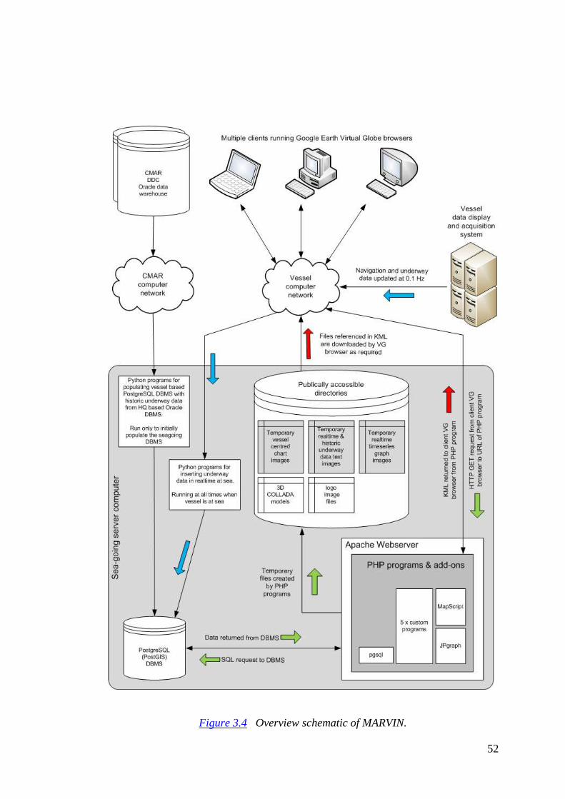
52
Figure 3.4 Overview schematic of MARVIN.

53
The use of OGC compliant geometries in MARVIN’s database for storing spatio-temporal
data collected in real-time, allows access to these data from full featured commercial and
desktop GIS software. This enables the use of desktop GIS software, for large format
printing of charts when time and expertise allows.
For instance, desktop GIS software can be used to produce projected and scaled paper charts
of the study area, based on ancillary datasets and the real-time data stored in MARVIN’s
database. Desktop GIS software such as uDig or ArcMap can access the same geometries
which are visualised by Google Earth. This enables the most suitable tool to be used for the
required task and removes the risk associated with creating multiple copies of evolving
datasets for multiple purposes.
With reference to Figure 3.4, the flow of spatio-temporal data within MARVIN can be
classified into the three paths detailed below.
• Underway data from vessel-mounted sensors are inserted into the MARVIN
database during a voyage in real-time every ten seconds by the vessel’s data
acquisition system. The positions versus time of deployed instruments are also
inserted into the database in real-time, limited by the update rate of the positioning
systems used (winch wire out measurements or USBL systems). Waypoint entries
detailing equipment deployment attribute details are inserted ad hoc via web forms.
These functions are shown blue in Figure 3.4.
• The MARVIN database is queried as required by a number of server-side PHP
scripts executed by the web server (Apache). The PHP scripts run on behalf of
Google Earth clients via HTTP requests to the web server when a KML Network
Link periodically refreshes. The scripts make use of the GIS functionality of the
spatially enabled database to undertake both spatial and / or temporal operations in
real-time. A number of temporary images, are created and stored in a publicly
accessible directory on the MARVIN server computer for later download. These
functions are shown green in Figure 3.4.
• The KML datastreams generated by the PHP scripts are streamed back to the client
computer running Google Earth. Google Earth parses the returned KML datastream
and updates its Virtual Globe display, reflecting changes and additions to spatio-
temporal data in the real-time database. Both the time stamping and geo-coding

54
abilities of KML are utilised in conjunction with Google Earth’s time control tool to
allow the user to view datasets in 4D. The temporary images for use by the
particular Google Earth client are downloaded as required. These functions are
shown red in Figure 3.4.
3.5.2 Database
Schema and Structure Query Language
As stated previously, the core of MARVIN is a PostgreSQL DBMS. PostgreSQL, in
conjunction with the PostGIS extension, enables the creation of a spatio-temporal database,
and a GIS. As well as storing spatio-temporal datasets, spatial and / or temporal operations
can be undertaken by the DBMS using Structured Query Language (SQL) operators.
The use of the SQL language for inserting, manipulating and retrieving data from
MARVIN’s database (via the DBMS) provides a simple but powerful mechanism for data
management. The SQL language has evolved over more than 20 years and provides an
extensive set of operators. The mature support within the SQL language for date and time
arithmetic is of great importance to this research.
The OGC standard OpenGIS Implementation Specification for Geographic information –
Simple feature access – Part 2: SQL option, details additional SQL operators which enable
spatial operations to be undertaken on spatial data within a database (Open Geospatial
Consortium Inc., 2005). The standard likewise details the mechanisms for storing spatial
data in a compliant geometry form. The PostGIS extension for PostgreSQL adheres to this
and other OGC standards, enabling spatio-temporal data to be stored, manipulated and
retrieved by the DBMS. The investigation of these abilities form an important part of the
research detailed in this thesis.
The collection of tables, columns, datatypes, and the relationships between columns in
different tables is referred to as a database’s schema. Figure 3.5 shows the simple database
schema utilised for this research. The basis of this schema was CMAR’s DDC data
warehouse. Of note is the use of the timestamp with timezone datatype for storing time
throughout the schema and the use of timestamps as the primary key for most tables. All
times are Universal Time Coordinates (UTC) and local time is never used. This is consistent
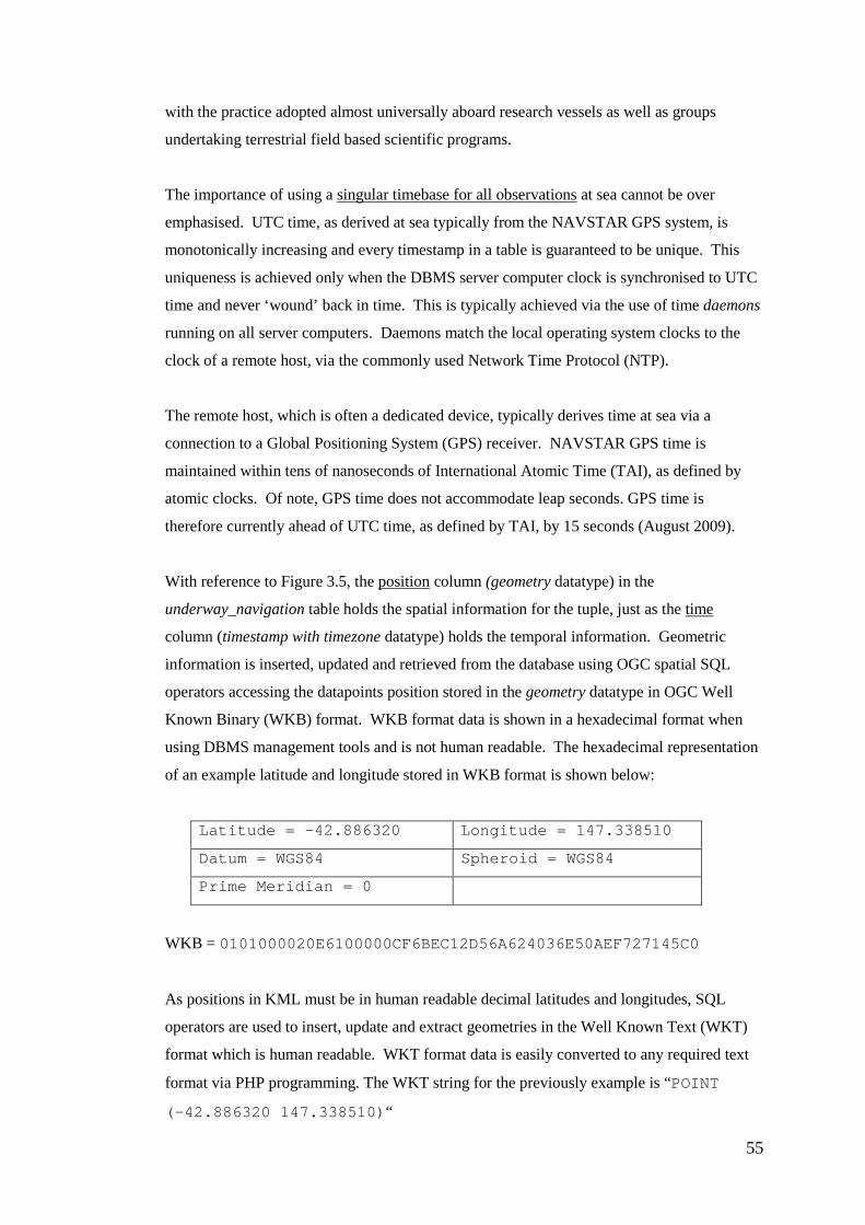
55
with the practice adopted almost universally aboard research vessels as well as groups
undertaking terrestrial field based scientific programs.
The importance of using a singular timebase for all observations at sea cannot be over
emphasised. UTC time, as derived at sea typically from the NAVSTAR GPS system, is
monotonically increasing and every timestamp in a table is guaranteed to be unique. This
uniqueness is achieved only when the DBMS server computer clock is synchronised to UTC
time and never ‘wound’ back in time. This is typically achieved via the use of time daemons
running on all server computers. Daemons match the local operating system clocks to the
clock of a remote host, via the commonly used Network Time Protocol (NTP).
The remote host, which is often a dedicated device, typically derives time at sea via a
connection to a Global Positioning System (GPS) receiver. NAVSTAR GPS time is
maintained within tens of nanoseconds of International Atomic Time (TAI), as defined by
atomic clocks. Of note, GPS time does not accommodate leap seconds. GPS time is
therefore currently ahead of UTC time, as defined by TAI, by 15 seconds (August 2009).
With reference to Figure 3.5, the position column (geometry datatype) in the
underway_navigation table holds the spatial information for the tuple, just as the time
column (timestamp with timezone datatype) holds the temporal information. Geometric
information is inserted, updated and retrieved from the database using OGC spatial SQL
operators accessing the datapoints position stored in the geometry datatype in OGC Well
Known Binary (WKB) format. WKB format data is shown in a hexadecimal format when
using DBMS management tools and is not human readable. The hexadecimal representation
of an example latitude and longitude stored in WKB format is shown below:
Latitude = -42.886320 Longitude = 147.338510
Datum = WGS84 Spheroid = WGS84
Prime Meridian = 0
WKB = 0101000020E6100000CF6BEC12D56A624036E50AEF727145C0
As positions in KML must be in human readable decimal latitudes and longitudes, SQL
operators are used to insert, update and extract geometries in the Well Known Text (WKT)
format which is human readable. WKT format data is easily converted to any required text
format via PHP programming. The WKT string for the previously example is “POINT
(-42.886320 147.338510) “

56
Figure 3.5 Database schema for the MARVIN PostgreSQL DBMS. (PK= primary key, FK = foreign key).
57
Population of database with historic underway data
Short scripts were written in the Python programming language to extract underway data
from the CMAR DDC Oracle data warehouse. All Southern Surveyor underway datasets for
2008 were extracted to large monthly Comma Separated Values (CSV) files. After the
creation of the MARVIN database schema, further Python scripts were used to populate the
new database with historic underway data.
The original tables in the Oracle-based data warehouse stored the latitude and longitude of
the vessel versus time in columns defined as floating point value datatypes. This method
was adopted for the new PostgreSQL database, but in addition, an extra column of geometry
datatype was added to the relevant tables and populated. When populating the
underway_navigation table in the database which contains the position of the vessel every
ten seconds versus time for the whole of 2009, the position column (geometry datatype) was
populated with the OGC WKB representation of the latitude and longitude values. This step
enabled the later use of OGC defined SQL spatial operators for spatial selection of subsets of
the spatio-temporal data. Refer to Chapter Two for further explanation of the advantages of
this method.
As well as enabling the use of spatial SQL operations and functions, storing coordinates in
the database in OGC compliant geometries allowed the use of PHP MapScript for generating
maps. MapServer CGI and PHP MapScript require geographical coordinates sourced from a
database to be stored as OGC geometries. Latitude and longitude values stored as floating
point values for instance, are not able to be utilised by MapServer or PHP MapScript for
mapping.
Population of database with real-time underway data
As well as populating the new MARVIN database with historic underway datasets, the
insertion of underway values in real-time was undertaken during two 2009 marine science
voyages. Small Python programs were used to decode bursts of underway data broadcast
from the Southern Surveyor’s data acquisition system via the vessel’s computer network.
Underway data was sampled and broadcast by the data acquisition system at 0.1 Hertz (a
sample every ten seconds), resulting in 8640 datapoints per 24 hour period, per underway
parameter.

58
The small server computer running the MARVIN server-side components described in
Section 3.2 was flown to Lautoka, Fiji in late June 2009 and installed aboard the Southern
Surveyor prior to Voyage three (SS2009_V03 Lautoka, Fiji to Noumea, New Caledonia).
During the voyage, the required Python scripts were completed and underway data at ten
second intervals were successfully inserted into the PostgreSQL database in real-time.
The MARVIN computer server subsequently stayed aboard for Transit two (SS2009_T02
Noumea, New Caledonia to Hobart, Australia), and continued to collect real-time underway
data directly into the MARVIN database. The computer was removed from the vessel in
Hobart in early August. These 2009 real-time collected underway datasets were used
alongside the 2008 historic underway datasets in support of this research.
Connection to the database
MARVIN Google Earth clients did not directly connect to the MARVIN DBMS and as such,
no log-in details needed to be entered by users to gain access. This was a design feature and
is typical of data acquisition, storage and display systems designed for use at sea on research
vessels. Typically, an individual’s or group’s participation on a research voyage implies the
willingness to provide fair access to datasets collected or derived by the individual or group.
Likewise, the individual or group benefits from being able to access datasets collected during
the voyage, by other individuals and groups participating on the voyage. Notwithstanding
this arrangement, data-use caveats and embargoes are often enforced as required.
The PHP scripts executed by the Apache web server connected to the MARVIN DBMS and
accessed datasets as required. The necessary log-in credentials were hard-coded in the PHP
scripts. Data within the database was selected and manipulated by the PHP scripts but never
changed. Further protection to data security was afforded by using a log-in account via PHP
which possessed read-only rights to the required tables.
Small Python scripts responsible for both the initial loading of the Southern Surveyor 2008
underway datasets, and the loading of underway data in real-time on the two 2009 voyages
described above, used log-in credentials which did permit write access to the required tables.
For data simulation purposes, the pgAdmin (http://www.pgadmin.org) tool was used on the
server. This was a convenient method allowing the creation of waypoint data and equipment
deployment data as required. PgAdmin is the standard GUI tool for the maintenance of a
PostgreSQL database. As described previously, the locations of waypoints and the times of

59
equipment deployments, recoveries and other significant events would typically be inserted
into MARVIN’s database at sea in real-time. Web-based forms or automatic processes
running on the vessel’s main data acquisition, logging and display system are typical sources
for waypoints.
Spatio-temporal operations within the DBMS
This section briefly gives some examples of spatio-temporal operations which were possible
within the DBMS by the use of the timestamp with timezone and geometry datatypes, for the
storage of temporal and spatial information respectively.
The storage of locations in the database as OGC geometries mandated the storage of datum,
spheroid and projection information with every datapoint in the MARVIN database. As
detailed previously, spatial operators added to the (PostgreSQL) standard SQL suite of
operators via the use of the PostGIS extension, allow the spatial selection and manipulation
of spatial data based on data in columns of the geometry datatype. Many operations
undertaken using SQL spatial operators required the stipulation of the datum, spheroid and
projection as part of the syntax. This allows the storage of data within the database in
unprojected geographic units, but the selection and conversion of the data into projected
units via SQL. Likewise, a datum shift can be undertaken in real-time on data selected by
the SQL spatial operators, rather than in another programming language which takes as
input, the results of the SQL query.
The specification of the datum, spheroid and projection of datapoints was accomplished
using EPSG codes. The International Association of Oil and Gas Producers (OGP) maintain
a list of numeric codes which uniquely identify a very wide range of combinations of
datums, spheroids and projections. These codes are commonly referred to as EPSG codes,
based on the former name of the OGP - European Petroleum Surveying Group. They are a
reliable method of specifying a unique combination of datum, spheroid and projection, and
are supported by many software packages which accommodate geospatial datasets. The
EPSG code used throughout this research was 4326. 4326 specifies a GRS80 spheroid,
WGS84 datum, and unprojected geographical units. This combination matches the positions
provided by the Konsgberg Seapath 200 NAVSTAR GPS receiver system which is the
primary navigation reference for the Southern Surveyor.
The combination of standard SQL operators and spatial operators (provided via PostGIS), in
conjunction with standard programming language functions, such as array searching and

60
ordering, and Boolean algebra, meant all GIS operations were undertaken wholly within the
MARVIN DBMS. Listed below are three simple examples of SQL queries used to
undertake some of the real-time spatio-temporal operations required within MARVIN
• Select current ship position
SELECT Astext(position) FROM underway_navigation WHERE time = current_db_time ORDER BY time DESC LIMIT 1
The Astext function converts the coordinate pair stored in the position column from
WKB format to readable WKT format in decimal latitude and longitude values as
required for use in KML. The WKT string POINT(147.33851 -42.88632) is returned
by this function, for a particular time.
As the EPSG code is associated within the database for this coordinate pair, it is
possible to select another datum, spheroid and / or projection for the recovered
coordinate pair and reproject ‘on-the-fly’. Hence, by substituting
Astext(transform(position, 28355)) into the above SQL query, the projection of the
returned coordinate pair would be Map Grid of Australia Zone 55 (MGA94, Z55).
For example, the Eastings and Northings returned would be “POINT( 527642
5251752)” for the same timestamp used above.
• Select all waypoints within a 5000 metre radius of the vessel
SELECT position FROM equipment_events, underway_navigation WHERE (equipment_events.time = underway_navigation.time) AND (distance_sphere(position, PointFromText(‘POINT(155.5 -32) ’, 4326))) < 5000)
The current position of the vessel (32º S, 155.5º E) is specified in the query. The
calculations are based on great-circle (as the crow flies) distances and there is no
need in PHP programs to undertake any spherical geometry operations. All
calculations are undertaken within the MARVIN DBMS via the SQL query.

61
• Calculate the great circle distance between the real-time vessel position and the
position of the last recovered fishing trawl
SELECT time, position, distance_sphere(position, PointFromText(‘POINT(155.5 -32)’, 4326)) FROM equipment_events, underway_navigation, equipment_actions, equipment_types WHERE (equipment_events.time = underway_navigation.time) AND (equipment_events.type_id = equipment_actions.type_id) AND (equipment_events.action_id = equipment_types.action_id) AND (type_description = ‘TRAWL’) AND (action_description = ‘RECOVERY’) ORDER BY time DESC LIMIT 1 This SQL query returns the time of and distance to, the location when the last fishing
trawl was recovered. As the location and speed of the vessel is updated in real-time
in the MARVIN database, it is possible to dynamically calculate estimated times of
arrivals (ETAs) for waypoints. All time and distance calculations can be undertaken
via the GIS functionality of the spatio-temporal of the MARVIN DBMS. Note the
necessary specification of the spheroid, datum and units via an EPSG code (4326).
As can be seen in the simple examples above, a range of GIS operations and calculations can
be undertaken wholly within MARVIN’s DBMS. The ability to undertake spatio-temporal
operations within a DBMS rather than via a programming language such as PHP greatly
simplifies data flow. This enables the programmer to concentrate on efficiency and
functionality, rather than being concerned with which Earth radius to use for great circle
calculations, for example.

62
3.5.3 Keyhole Markup Language
Introduction
The use of the Keyhole Markup Language was a key component of MARVIN and the
research undertaken and presented here. As previously outlined, KML was evaluated in this
research as the data format for information sent between the server-side processes
manipulating spatio-temporal data (in the DBMS) and the client-side Virtual Globe browser
visualising spatio-temporal datastreams.
KML is based on the Extensible Markup Language (XML) for encoding geographic data.
Briefly, XML files are human readable text files consisting of characters divided into
markup and content elements. Markup elements are words which are enclosed by greater
than and less than symbols in the code. A start-tag and end-tag pair such as <name>John
</name> is an example of markup elements. John is a content element in this case. Hence,
name has been specified to be equal to John. An attribute can be associated with a tag such
as <name type=christrian>John </name>.
KML’s long list of elements allowing the encoding of geographic data are KML-specific
XML markup elements. For instance, <heading>, <latitude> and <longitude> elements
within a KML file specify the data required by a <Camera> element, where the <Camera>
element describes the viewpoint and from which to create a 3D view.
Importantly and necessarily for this research, KML supports both negative and positive
elevations (depths and heights) as well as the time component of spatial objects. KML also
allows symbology information to be included which can be used by software packages
accessing a KML dataset.
Regardless of the software package used to open a KML document, identical symbology
should ideally be used. For example, the symbology used to create the visualisations of data
contained in a correctly formatted KML document should ideally appear the same, when
opened with desktop GIS software (ArcMap or MapInfo) and a Virtual Globe browser
(Google Earth or Worldwind). For example, major roads would appear as thick orange lines
and lakes would appear as blue filled polygons.
63
This is in contrast to common geographic data exchange formats such as E00 (ESRI) and
DXF (Autocad) which provide no or limited support for the inclusion of symbology data.
TAB (MapInfo - Pitney Bowes) format files are able to store symbology data specifying line
thickness or fill colour for example, but they lack the ability to associate timestamps to
individual geographic objects.
A full description of the KML 2.2 syntax is not included here for brevity. Interested readers
are directed to the Open Geospatial Consortium webpage (http://web.opengeospatial.org) for
access to standards documents.
Descriptions of specific KML elements used
MARVIN used a variety of KML elements to describe the spatio-temporal datasets extracted
from the database. Listed below are brief descriptions of the important KML elements used
as part of this research, and the functionality they provided.
<Model> element
The <Model> element provides a mechanism to describe the position of a 3D model of
an object, in both space and (optionally) time. The 3D position, along with the scale,
heading, roll and tilt of the model can be specified. The path to a COLLADA
(https://collada.org) format model needs to be specified, allowing the Virtual Globe
browser to access the model as required. Figure 3.6 shows some of the models of real
world objects utilised by MARVIN.
A COLLADA model is an XML encoded text file format defining the vertices, facets,
textures and colours of a 3D model of an object. The file format makes the exchange
of 3D models between packages which generate 3D models, such as Google Sketch
Up (http://sketchup.google.com) and Autodesk 3D Studio Max
(http://usa.autodesk.com), possible via an open-source standard (Wernecke 2009).
The <Model> element was used extensively in MARVIN for positioning models of the
vessel and deployed equipments. The ability to change the scale of the model as
displayed in the Virtual Globe browser, allowed the same model to be shown at
multiple scales, making small objects in a large ocean easier to locate in Google Earth.

64
Figure 3.6 Examples of simple COLLADA models of a vessel (left) and water sampling
equipment (right) usable in MARVIN.
<ScreenOverlay> element
The <ScreenOverlay> element allows the overlay of an image file on the Google Earth
screen. The path to the image file to be overlaid and its position can be specified. The
position can be expressed in pixels or as a fraction of the Google Earth screen width,
accommodating varying desktop sizes for clients.
The <ScreenOverlay> element was used in MARVIN to embed images showing time-
series graphs of underway datasets, small vessel-centred planimetric charts, and
images of real-time and historic textual data, such as UTC time and vessel location.
<TimeSpan> element
KML’s ability to accommodate the time component of spatial data is provided by the
<TimeSpan> element. This simple element allows the specification of the valid start
and end times for an object to exist in a location. Time is specified using the ISO8601
convention, and can be specified using reduced formats.
(http://www.iso.org/iso/date_and_time_format#what-iso-8601-covers)
For example, an object can be specified to exist in 3D space between two times, such
as 2009-01-01T00:00:00+00 and 2009-01-02T00:00:00+00. This forces Google
Earth to only show the object when the time selector is set to a time during the 1st of
January 2009. The ability within KML to exactly specify time periods for which the
3D location of an object is valid is a key reason for its suitability for use within spatio-
temporal data exploration techniques.
The <TimeSpan> element was used extensively in MARVIN to accommodate the
varying positions versus time of the vessel and deployed instruments. Hence, a

65
timestamp was associated with each position in the KML datastreams. This allowed
the replay of historic data, which in turn allowed the positioning of models of the
vessel and deployed instruments according to a user determined epoch.
3.5.4 Temporary files
Temporary files were utilised extensively in MARVIN in support of the dynamically
generated KML datastreams. The use of temporary files is commonplace when serving
dynamic or customised data via web servers to multiple clients. An example of this is the
creation of temporary image files (in GIF or PNG format) by remote web mapping software
such as MapServer.
For example, each new client (web browser) accessing a web mapping site can send a list of
the required layers, spatial coverage and symbology, using a HTML form. These user
controlled settings are passed to the map server via variables embedded in the Universal
Resource Locator (URL). The remote web mapping application creates a map (as an image)
meeting the client specifications and saves the image file (e.g. GIF or PNG) to a publicly
accessible location, using a random filename. The URL to this temporary file is passed back
to the client via HTML. The client in turn, downloads the file and displays it via the web
browser.
This process repeats itself for every pan, zoom or selection of layers undertaken through the
web browser running on each client. A busy web mapping site may generate thousands of
temporary randomly named image files for use by dozens of simultaneous clients per hour.
The publicly accessible directory containing these temporary files is typically purged of files
older than a few hours on a daily or more frequent basis.
Temporary image files used as part of the research detailed here, were created as 24-bit PNG
images by PHP server-side programs and saved to publicly accessible directories within the
MARVIN web server directory structure. The temporary image files were downloaded by
Google Earth upon parsing of the KML datastream, which referenced the particular image
files via the embedded random filename(s).

66
Temporary image files were utilised during the course of this research to fulfill the four
needs described below. The image files were embedded into the Virtual Globe browser GUI
via the ScreenOverlay method described in the previous section.
Time series graphs
The availability of historic underway parameters in the MARVIN database made possible
the creation of time series graphs. Time series graphs of parameters such as humidity, wind
speed or photosynthetic active radiation, are often created regularly during a marine research
voyage for quality control purposes. The loss of a blade from the impellor of an
anemometer, or the fogging of the dome of an upward looking radiation sensor, is much
more easily detected when data are viewed as time series graphs rather than tabulated values.
This is especially true for research vessels that carry identical instruments located on the port
and starboard for redundancy or to reduce shading (of light or wind).
Within MARVIN, time series graphs of underway parameters of interest were created using
PHP and the JpGraph module. By embedding a time series graph in the Google Earth GUI,
it was possible to link parameters, which varied in space and time, to a view showing not
only when, but importantly where an empirical measurement was taken.
This is a often a requirement when reviewing or analysing spatio-temporal datasets of a
parameter such as sea surface temperature or salinity measured at sea on a moving platform.
Both the time and the location of the measurement are important and both should be
accommodated when presenting datasets as graphs or charts. As previously mentioned, the
graphing capabilities of JpGraph are very good and it was possible to create simple, well
formatted time series graphs of underway parameters (refer to Figure 3.1).
Real-time vessel underway data – tabulated text
For real-time operation, there was a need to show current UTC time, vessel position, speed
and heading via MARVIN in the Google Earth main window. The ability to reliably report
the current UTC time and vessel position is a primary function of real-time applications such
as MARVIN. As previously mentioned, the use of UTC time at sea is the norm and all
events of scientific significance are almost always logged in UTC time.

67
JpGraph was used to create small PNG format images. The images contained real-time
values of UTC date and time, vessel position, COG, SOG and depth, embedded as text. The
background colour of the new image created every ten seconds, was changed to give
confidence to the user that the values displayed were updated in real-time. The images were
saved on the MARVIN server and downloaded by the Google Earth clients for display as
required. Figure 3.7 shows a set of images generated by this method.
Figure 3.7 Example of six successive JpGraph generated images containing real-time
underway data as text. Each image is displayed for ten seconds in the Google Earth main
window, before being replaced with a newer image.
Historic vessel underwater data – tabulated text
As one of the main goals of this research was to evaluate the accommodation of time within
KML, there was a need to be able to play back historic spatio-temporal datasets, using the
Google Earth time control.
As well as positioning the vessel model, and icons or models representing deployed
instruments, in the correct space and time, there was a need to be able to display UTC time
and relevant underway data, as collected at a user determined historic epoch. The resulting
system should enable an interested user to move through time at will, observing the position
of the vessel and deployed instruments, whilst simultaneously viewing tabulated underway
parameters collected at the time and / or position of interest.
The same JpGraph based process described above for displaying real-time underway data as
images of text, was adopted for displaying historic underway data text. Figure 3.8 shows a
typical set of images generated via this process for a three minute period. Of note is the

68
requirement to generate a temporary image containing text data for every epoch returned in a
KML datastream. For instance, if a KML datastream enables the replay of the previous six
hours of underway data in Google Earth, temporary images containing the text of the
required underway parameters at each of the ten second intervals within the six hour window
must be created.
Hence, the KML datastream returned to Google Earth would reference 2160 temporary
images created via a PHP program in conjunction with JpGraph. Each of these 2160 images
is displayed in succession as the Google Earth time slider moves through time.
Figure 3.8 Example of JpGraph generated images containing historic underway text. The nine images shown would be displayed in turn in the Google Earth main window, as the time
advances in the time control. Each image is valid for a twenty second period.
Planimetric charts
By design, a Virtual Globe browser such as Google Earth permits a 3D-like view of the
surface of the Earth, on a 2D computer screen. The strengths of Virtual Globes include the
ability to look at a location on the Earth’s surface in 3D space from a desired direction and
altitude. This implies North can no longer be relied upon to lay in a particular direction on
the computer screen. Virtual Globe browsers generally include an on-screen compass to
assist the user in maintaining their bearing as they ‘fly’ through space, and potentially time.
Whilst these features are the very strengths of Virtual Globe, they can be at odds with
conventional cartographic technique. GIS users are very familiar with viewing spatial
datasets in 2D on a computer monitor with the relevant North direction aligned with the edge
of the computer display and pointing up. Likewise, planning for fieldwork sorties and
marine science voyages is often undertaken using GIS based or paper, charts and maps.

69
These large format paper charts are invariably taken to sea and continue to be added to,
either via GIS or hand drawn annotation.
Given the reliance on standard hydrographic charts on research vessels and the availability of
remotely sensed imagery useful to many marine based studies, there was a requirement when
building MARVIN to embed a planimetric view in the Google Earth browser, centred on the
real-time position of the vessel. This enabled the creation of simple charts which were
always centred on the current position of the vessel, always had True or Grid North facing
aligned up the computer screen and was always at a set scale. This consistency is
advantageous when working simultaneously with paper charts, 2D GIS and a 4D tool such as
Google Earth, when all three techniques are used to view the same geographical area.
To implement this feature, a process similar to the one described above for the generation of
PNG images containing time series graphs was adopted. Rather than using PHP in
conjunction with JpGraph, PHP in conjunction with the Mapscript module was utilised.
PHP Mapscript was used to access the functionality of the MapServer libraries installed on
the MARVIN server. This permitted the creation of a series of PNG format images (of
predefined charts), centred over the vessel’s current location. The scale and symbology of
the charts were defined in configuration files on the MARVIN server. A set of small
temporary PNG format images of vessel centred charts were created every ten seconds for
every Google Earth client accessing MARVIN. Two charts were selected by the user as
required for display in Google Earth, via the side bar.
As previously mentioned, Mapscript enabled PHP programs are able to connect to a
PostgreSQL database and utilise locations stored as OGC compliant geometries. Both
historic and real-time underway datasets in the MARVIN database, as well as ancillary
datasets, such as waypoint locations, utilised the geometry datatype for the storage of
locations. This enabled the relevant PHP program access to position information from the
MARVIN database for the creation of charts centred on the vessel’s real-time position. This
functionality is discussed further in Chapter Four.
Figure 3.9 shows three example images created via this technique. Of note is the ability to
produce vessel centred planimetric charts, using differing projections and scales which can
be viewed simultaneously in the Google Earth browser. The significance of this feature is
discussed in the next chapter.

70
Figure 3.9 Examples of PHP Mapscript generated, vessel-centred planimetric charts. Plate carrée MODIS sea surface temperature (top), plate carrée illuminated DEM (middle), and
UTM projected metric range rings (bottom)
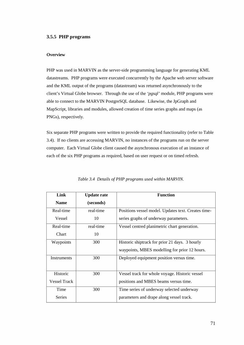
71
3.5.5 PHP programs
Overview
PHP was used in MARVIN as the server-side programming language for generating KML
datastreams. PHP programs were executed concurrently by the Apache web server software
and the KML output of the programs (datastream) was returned asynchronously to the
client’s Virtual Globe browser. Through the use of the ‘pgsql’ module, PHP programs were
able to connect to the MARVIN PostgreSQL database. Likewise, the JpGraph and
MapScript, libraries and modules, allowed creation of time series graphs and maps (as
PNGs), respectively.
Six separate PHP programs were written to provide the required functionality (refer to Table
3.4). If no clients are accessing MARVIN, no instances of the programs run on the server
computer. Each Virtual Globe client caused the asynchronous execution of an instance of
each of the six PHP programs as required, based on user request or on timed refresh.
Table 3.4 Details of PHP programs used within MARVIN.
Link
Name
Update rate
(seconds)
Function
Real-time
Vessel
real-time
10
Positions vessel model. Updates text. Creates time-
series graphs of underway parameters.
Real-time
Chart
real-time
10
Vessel centred planimetric chart generation.
Waypoints 300 Historic shiptrack for prior 21 days. 3 hourly
waypoints, MBES modelling for prior 12 hours.
Instruments 300 Deployed equipment position versus time.
Historic
Vessel Track
300 Vessel track for whole voyage. Historic vessel
positions and MBES beams versus time.
Time
Series
300 Time series of underway selected underway
parameters and drape along vessel track.
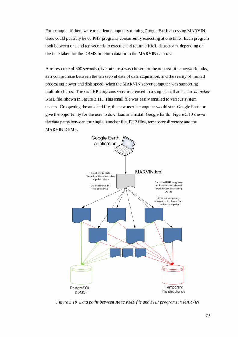
72
For example, if there were ten client computers running Google Earth accessing MARVIN,
there could possibly be 60 PHP programs concurrently executing at one time. Each program
took between one and ten seconds to execute and return a KML datastream, depending on
the time taken for the DBMS to return data from the MARVIN database.
A refresh rate of 300 seconds (five minutes) was chosen for the non real-time network links,
as a compromise between the ten second date of data acquisition, and the reality of limited
processing power and disk speed, when the MARVIN server computer was supporting
multiple clients. The six PHP programs were referenced in a single small and static launcher
KML file, shown in Figure 3.11. This small file was easily emailed to various system
testers. On opening the attached file, the new user’s computer would start Google Earth or
give the opportunity for the user to download and install Google Earth. Figure 3.10 shows
the data paths between the single launcher file, PHP files, temporary directory and the
MARVIN DBMS.
Figure 3.10 Data paths between static KML file and PHP programs in MARVIN
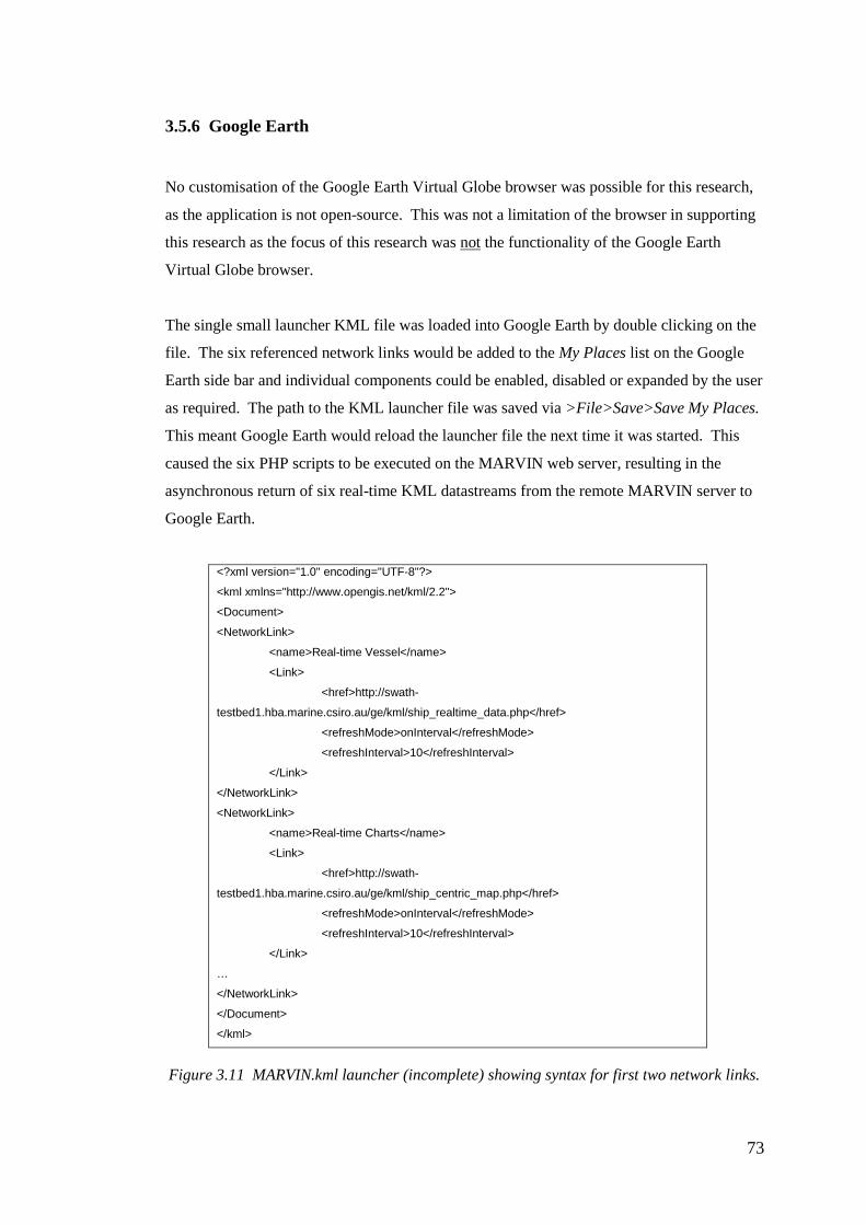
73
3.5.6 Google Earth
No customisation of the Google Earth Virtual Globe browser was possible for this research,
as the application is not open-source. This was not a limitation of the browser in supporting
this research as the focus of this research was not the functionality of the Google Earth
Virtual Globe browser.
The single small launcher KML file was loaded into Google Earth by double clicking on the
file. The six referenced network links would be added to the My Places list on the Google
Earth side bar and individual components could be enabled, disabled or expanded by the user
as required. The path to the KML launcher file was saved via >File>Save>Save My Places.
This meant Google Earth would reload the launcher file the next time it was started. This
caused the six PHP scripts to be executed on the MARVIN web server, resulting in the
asynchronous return of six real-time KML datastreams from the remote MARVIN server to
Google Earth.
<?xml version="1.0" encoding="UTF-8"?>
<kml xmlns="http://www.opengis.net/kml/2.2">
<Document>
<NetworkLink>
<name>Real-time Vessel</name>
<Link>
<href>http://swath-
testbed1.hba.marine.csiro.au/ge/kml/ship_realtime_data.php</href>
<refreshMode>onInterval</refreshMode>
<refreshInterval>10</refreshInterval>
</Link>
</NetworkLink>
<NetworkLink>
<name>Real-time Charts</name>
<Link>
<href>http://swath-
testbed1.hba.marine.csiro.au/ge/kml/ship_centric_map.php</href>
<refreshMode>onInterval</refreshMode>
<refreshInterval>10</refreshInterval>
</Link>
…
</NetworkLink>
</Document>
</kml>
Figure 3.11 MARVIN.kml launcher (incomplete) showing syntax for first two network links.

74
Chapter 4 Results
This chapter describes the functionality of MARVIN. The suitability of the combined
technologies researched is shown by the level of functionality achievable in MARVIN. As
previously outlined, the two main technologies researched were a spatio-temporal DBMS
and the KML language. The particular application was the use of these technologies in
visualising real-time spatio-temporal marine data in a multi-user environment at sea.
As MARVIN is a computer based application, and particularly as it is a very visual
application, descriptions and figures within this chapter are best supplemented by ‘hands-on’
use. Downloadable KML files have been made available which can be used with your
Google Earth browsers. These files allow the ‘offline’ evaluation of MARVIN as they are
static KML files which will not refresh from a remote DBMS via network links. Images of
many of the larger figures are also provided. The URL for access is listed below:
http://www.users.on.net/~opus405/masters_thesis
Interested readers are strongly encouraged to access the figures and KML files. The use of
the KML files in Google Earth will be of benefit to interested readers in understanding the
uses of MARVIN.
The KML files available for download assume a desktop resolution of at least 1600 x 1200
pixels. Use of a lower resolution desktop may cause some overlap of the time series, charts
and text, image overlays in the Google Earth main window. Individual image overlays can
be turned on and off as required via the side bar, should a 1600 x 1200 desktop not be
available.
A concise description of MARVIN is best undertaken in sections. The functionality
described within each of the following sections is provided by a single network link
embedded in the single small KML launcher file which starts MARVIN (MARVIN.kml).
Each of the network links references a PHP program, executed by the web server software
each time the link is refreshed, as was previously described in Chapter Three.
The final section of this chapter contains a series of scenarios which detail how MARVIN
might typically be used at sea during a research voyage.

75
4.1 Introduction to MARVIN
Figure 4.1 MARVIN’s six
network link icons.
Interaction with MARVIN was undertaken via the Google
Earth side bar. Each of the six main Network Links could
be enabled and disabled as required. Figure 4.1 shows the
six network links: Real-time Vessel; Real-time Charts;
Waypoints; Instruments; Historic Vessel Track and Time
Series. The link icons coloured yellow shown in Figure
4.1 were in the process of waiting for a datastream from
the MARVIN server when this screen capture was made.
Layers and folders of layers, are stored within each of the six network link folders.
Individual layers, or folders of layers, could be turned on and off to suit user requirements.
After initially loading the small KML launcher file to start MARVIN, the six network links
described in the following sections refreshed for the first time. The layers within each
network link folder which were initially enabled, when starting MARVIN from Google
Earth, were set by the PHP programs running on the MARVIN server. This prevented
overlapping layers from appearing in the Google Earth when starting a new session. Figure
4.2 shows an overview of all MARVIN layers selectable through the Google Earth side bar.
Each of the six network links would periodically refresh at the interval set in the small KML
launcher file. The two real-time network links were configured to refresh every ten seconds.
This interval matched the real-time underway data logging rate of the Southern Surveyor
data acquisition system. The remaining four network links were configured to refresh every
five minutes as has been described in Section 3.5.5.
Network links could be easily refreshed manually if desired by right-clicking the icon for the
network link and selecting the Refresh option. A manual refresh of a network link might be
advantageous to a user after entering a number of new waypoints into the MARVIN database
from a web form, for example. To quickly validate the position of these new waypoints,
users could force the reload of the Waypoints network link.
As MARVIN was designed to be a multi-user system, the layers turned on and off in one
Google Earth client did not affect other clients. All clients could concurrently access the
same real-time datasets sourced from MARVIN’s database. The symbology used on all
clients accessing MARVIN was identical. The symbology was set in the six PHP programs

76
and their associated shared modules. It was possible via Google Earth to change the
symbology used for a layer by right clicking on an icon and selecting a different colour or
line thickness, for example. However, this user preference was overwritten when the
network link which provided the data for a layer refreshed. This enforced consistency across
multiple clients, ensuring vessel tracks were always the same colour, and the same icon was
always used for a particular piece of equipment, for example.
Figure 4.2 Overview of MARVIN layers, as shown in the Google Earth side bar.

77
4.2 Real-time Vessel network link
Figure 4.3 Real-time Vessel
network link icons.
The Real-time Vessel network link provided the main
real-time functionality of MARVIN (refer to Figure
4.3).
This link positioned and updated, models of the vessel,
modelled Multi-Beam Echo-Sounder beams, an image
of text of real-time underway data, and models and
icons representing deployed equipment positions.
Figure 4.4 shows a screen capture of MARVIN with
all network links turned off apart from the Real-time
Vessel network link.
Figure 4.4 Google Earth screen capture showing small vessel model. The real-time
underway data displayed in the top right hand corner of the figure shows the UTC date as
10th October 2008. This was day one of Voyage 10, 2008, departing Sydney.

78
Both a correctly scaled model, and a much larger not-to-scale model of the vessel were
positioned in real-time. The correctly scaled model shown in Figure 4.4, was most useful
when working close to shore, where the vessel model was likely to be viewed in conjunction
with Google supplied models, and high spatial resolution imagery.
A much larger vessel model positioned at altitude, assisted in finding the vessel when using
MARVIN at sea, away from any Google supplied models or when the viewing altitude set by
the user was large (refer to Figure 4.5). Likewise, a yellow vertical line extending from the
model’s navigation reference point to the actual real-time position was useful for showing
the position of the scaled vessel model, once the large model had been located.
The small and large vessel models and the vertical yellow line could be turned on and off
individually as required via the Google Earth side bar. In practice, the large vessel model
was not generally enabled.
Figure 4.5 Large vessel model.
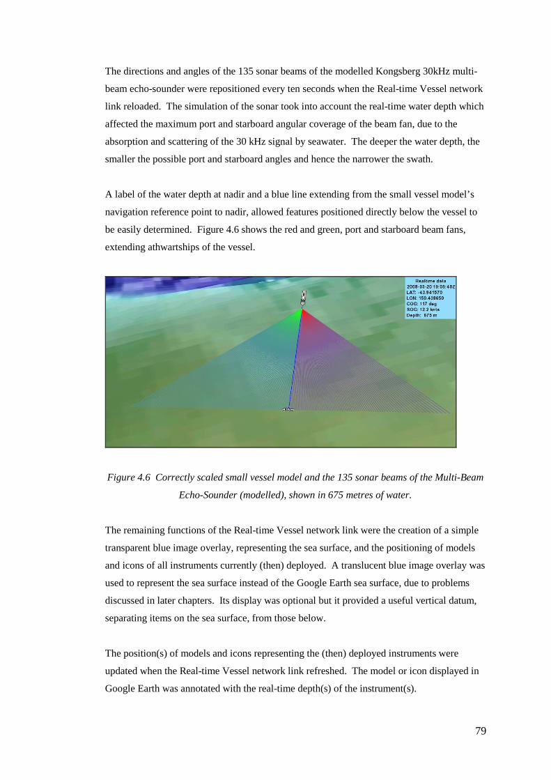
79
The directions and angles of the 135 sonar beams of the modelled Kongsberg 30kHz multi-
beam echo-sounder were repositioned every ten seconds when the Real-time Vessel network
link reloaded. The simulation of the sonar took into account the real-time water depth which
affected the maximum port and starboard angular coverage of the beam fan, due to the
absorption and scattering of the 30 kHz signal by seawater. The deeper the water depth, the
smaller the possible port and starboard angles and hence the narrower the swath.
A label of the water depth at nadir and a blue line extending from the small vessel model’s
navigation reference point to nadir, allowed features positioned directly below the vessel to
be easily determined. Figure 4.6 shows the red and green, port and starboard beam fans,
extending athwartships of the vessel.
Figure 4.6 Correctly scaled small vessel model and the 135 sonar beams of the Multi-Beam
Echo-Sounder (modelled), shown in 675 metres of water.
The remaining functions of the Real-time Vessel network link were the creation of a simple
transparent blue image overlay, representing the sea surface, and the positioning of models
and icons of all instruments currently (then) deployed. A translucent blue image overlay was
used to represent the sea surface instead of the Google Earth sea surface, due to problems
discussed in later chapters. Its display was optional but it provided a useful vertical datum,
separating items on the sea surface, from those below.
The position(s) of models and icons representing the (then) deployed instruments were
updated when the Real-time Vessel network link refreshed. The model or icon displayed in
Google Earth was annotated with the real-time depth(s) of the instrument(s).

80
4.3 Real-time Charts network link
Figure 4.7 Real-time Charts
network link icons
The Real-time Charts network link provided control of a
pair of vessel-centred, planimetric charts, embedded in
the Google Earth main window as image overlays. The
image overlays could be turned on and off independently
as desired via the Google Earth side bar as shown in
Figure 4.7.
The upper chart in the Google Earth main window (refer
to Figure 4.8) always used a plate carrée projection,
matching the simple projection often used for satellite
derived imagery of sea surface temperature or ocean
colour. The lower chart always used a Universal
Transverse Mercator projection.
The lower chart was intended for use when the vessel was working close to waypoints,
undertaking equipment deployments and retrievals so working in ground units (such as
metres or Nautical Miles) rather than fractions of degrees was a requirement. The speed and
direction of vessel drift over time, due to wind and water currents, is often of interest at
navigationally challenging times. The UTM zone and hemisphere for the lower chart were
automatically chosen to suit the position of the vessel, by server-side software. The ability to
maintain vessel heading and position is referred to as a vessel’s station keeping ability.
Good station keeping ability is essential for vessels which routinely deploy profiling
instruments over their stern or sides, especially in marginal sea conditions such as when
winds or water currents are strong.
Both the upper and lower embedded charts possessed options controllable via the Google
Earth side bar. The upper chart background image was selectable as: a raster navigation
chart (ENC) from the Australian Hydrographic Service; a Geoscience Australia sun
illuminated DEM; or a Moderate Resolution Imaging Spectroradiometer (MODIS) sea
surface temperature image. The lower chart had no background image but the user could
select one of four geographical extents for the chart. At small scales, the size of the blue
icon representing the vessel outline was scaled correctly within the 400m x 400m extents of
the lower chart. The length of the blue icon on the computer screen represented the 65 metre
length of the Southern Surveyor.
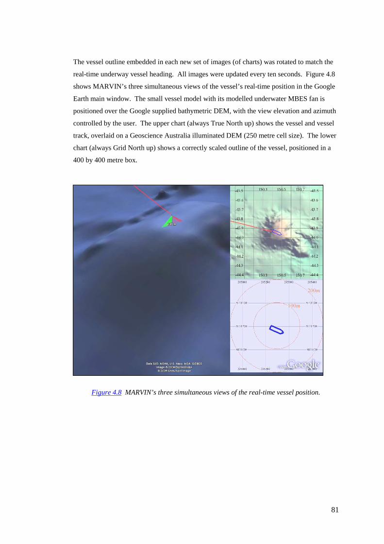
81
The vessel outline embedded in each new set of images (of charts) was rotated to match the
real-time underway vessel heading. All images were updated every ten seconds. Figure 4.8
shows MARVIN’s three simultaneous views of the vessel’s real-time position in the Google
Earth main window. The small vessel model with its modelled underwater MBES fan is
positioned over the Google supplied bathymetric DEM, with the view elevation and azimuth
controlled by the user. The upper chart (always True North up) shows the vessel and vessel
track, overlaid on a Geoscience Australia illuminated DEM (250 metre cell size). The lower
chart (always Grid North up) shows a correctly scaled outline of the vessel, positioned in a
400 by 400 metre box.
Figure 4.8 MARVIN’s three simultaneous views of the real-time vessel position.

82
4.4 Waypoints network link
Figure 4.9 Waypoints
network link icons.
The Waypoints network link allowed display of both
equipment waypoints and three hourly waypoints, for a
voyage. The names of waypoints were a concatenation
of the equipment type identifier, (CAM for camera
deployment, DRE for dredge and so on), and a unique
three digit numeric sequence number, as shown in
Figure 4.9.
For test purposes, waypoint information was directly
entered into the simulated_deployments table in the
MARVIN database, using the pgadmin tool as
described in the previous chapter.
In reality, waypoint data would typically be entered during a research voyage via web-based
forms, allowing the multi-user entry, editing and display, of waypoint data in a tabular
format. The insertion of waypoint data into the MARVIN database can also be expected to
be undertaken automatically in some circumstances. For example, software responsible for
the control and logging of data, from individual instruments such as CTDs, is often capable
of broadcasting times of events, such as the equipment reaching the seabed, or the
commencement of data logging.
Balloon pop-up windows were available for all waypoints in MARVIN. Figure 4.10 shows
an example of a dredge deployment and recovery, and the results of clicking on the waypoint
icon located at the deployment location. The vertical green and red lines show the locations
and times of equipment deployment and recoveries respectively. The white lines show the
path of the instrument through the water column, and on the seabed in the case of
instruments such as a dredges or benthic sleds. The times and dates of events such as
‘touching down’ and ‘lifting off’ the seabed, are derived from values in the
simulated_deployments table in the MARVIN database, and are shown in Google Earth.
Knowledge of these times allows swept areas and volumes to be calculated during
subsequent analysis stages if desired, for example.
The name used for labeling the three hourly observations was the UTC time of observation.
Three hourly positions were automatically derived directly from the ten second interval

83
underway dataset stored in MARVIN’s database. The three hour interval represented a
compromise between displaying too many icons or too few.
Figure 4.10 Example of a pop-up balloon associated with a waypoint. The underwater path
of dredge 212 through the water column is shown as thin white lines. The path of the dredge
up the continental slope, is shown as a large white line draped on the seabed DEM.
Figure 4.11 shows the pop-up balloons available in MARVIN for three equipment types.
The names shown are a concatenation of the equipment type identifier and a unique three
digit numeric sequence number, as has been preciously explained. Figure 4.11 therefore
shows pop-up balloons for Beam Trawl 170, Bongo Net 160 and Conductivity and
Temperature Depth instrument 150. Importantly, pop-up balloons allowed an overview of
waypoint data and easy access to URL(s) pointing to non-KML datasets (shown as ‘link to
profiles’ in the balloon shown in Figure 4.11). These datasets could for example, include
large graphic images of individual Conductivity Temperature and Depth instrument vertical
profiles, directories of images downloaded from a stills camera, or a scanned paper logsheet
for a rock dredge deployment.
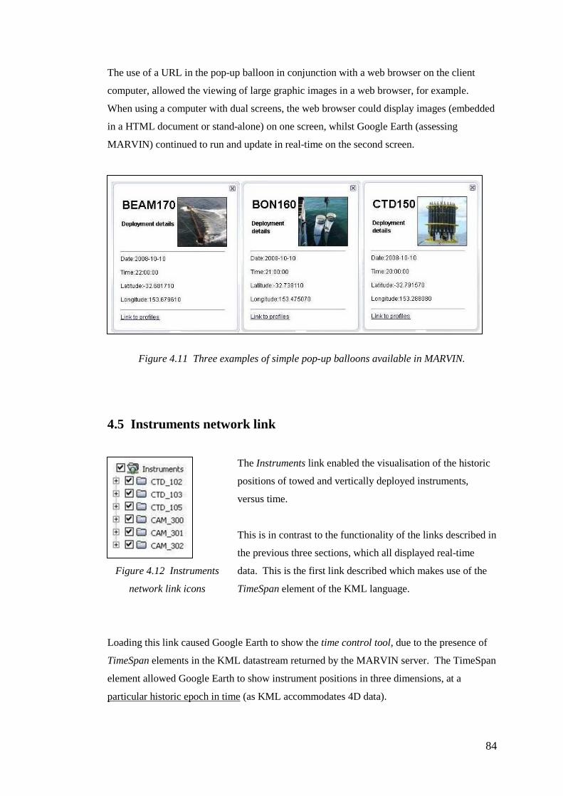
84
The use of a URL in the pop-up balloon in conjunction with a web browser on the client
computer, allowed the viewing of large graphic images in a web browser, for example.
When using a computer with dual screens, the web browser could display images (embedded
in a HTML document or stand-alone) on one screen, whilst Google Earth (assessing
MARVIN) continued to run and update in real-time on the second screen.
Figure 4.11 Three examples of simple pop-up balloons available in MARVIN.
4.5 Instruments network link
Figure 4.12 Instruments
network link icons
The Instruments link enabled the visualisation of the historic
positions of towed and vertically deployed instruments,
versus time.
This is in contrast to the functionality of the links described in
the previous three sections, which all displayed real-time
data. This is the first link described which makes use of the
TimeSpan element of the KML language.
Loading this link caused Google Earth to show the time control tool, due to the presence of
TimeSpan elements in the KML datastream returned by the MARVIN server. The TimeSpan
element allowed Google Earth to show instrument positions in three dimensions, at a
particular historic epoch in time (as KML accommodates 4D data).

85
The epoch was user selectable via the Google Earth time control tool. Figure 4.13 shows the
time control tool in the upper left hand corner. The position and depth of all deployed
instruments is shown for the time 11th October 2009 21:12:00 UTC, as selected by the user
via the time control tool.
Figure 4.13 shows the position and depth of a single profiling instrument below the vessel at
the desired epoch. The instrument’s position is shown in Google Earth by an icon
representing the instrument type. The depth and position of the instrument versus time, was
recovered from the MARVIN database. 4D positions for profiling and towed instruments
were modelled in the database for research purposes. In reality, these positions would be
automatically input into the MARVIN database in real-time, sourced from systems such as
USBL or winch wire-out measurements (as explained in Chapter Two). The position of the
vessel model, and the values displayed in the image containing text showing historic
underway data in the Google Earth main window, are also correct for the historic epoch
selected. This functionality is explained in the next section (Historic Shiptrack link).
Figure 4.13 Google Earth time control tool used for determining the position of a vertical
profiling instrument, represented by a penguin icon, at a particular historic time.

86
The ability to easily overlay the position of underwater instruments versus time on a 3D path
enables visual analysis of many aspects of underwater instruments. For example, viewing
the flight of a new fishing net or towed camera system through the water column, given
particular winch and vessel speeds is useful. The initial trial deployments of an instrument
assist in developing standard operating procedures and the ability to view the 3D paths of
new nets or equipment, in conjunction with vessel speed and heading, and underway
parameters in invaluable.
The Instruments network link in MARVIN enabled the replay of equipment position and
flights, during and after, an instrument’s deployment and recovery, with very little user
intervention.

87
4.6 Historic Vessel Track network link
Figure 4.14 Historic Vessel
Track network link icons.
The Historic Vessel Track network link was the
second network link to make use of the KML
TimeSpan element.
This network link displayed historic underway data
as an image of text, historic vessel position and
modelled historic multi-beam echo-sounder beams, at
a user determined epoch.
As per the link described above, when the Historic Vessel Track link was enabled in the
Google Earth side bar (refer Figure 4.14), the time control tool would become accessible in
the main window, as shown in the top left-hand corner Figure 4.15
This network link also generated two vessel tracks which showed the path of the vessel from
the start of the voyage, to the (then) present time. Red and yellow tracks were drawn on the
sea surface and seabed DEM respectively. It was also possible to display a ‘curtain’ or
‘drape’, extruded between the red sea surface track and the yellow seabed track. The curtain
made it very easy to visualise the along-track depth profile beneath the vessel track, as user
view azimuth and elevation were varied in Google Earth. Figure 4.15 shows the path of the
vessel across the continental slope from the start of the voyage to the (then) present time.
The position of the historic vessel model, and the values of historic underway data, shown as
an image of text, are determined by the time set via the time control tool (shown in the top
left-hand corner of the Figure 4.15).
The historic vessel model used by this link was coloured red, indicating the position of the
vessel model did not represent the real-time position of the vessel. Both real-time and
historic vessel models could be displayed in the Google Earth main window together. In
general use, the vessel and multi-beam echo sounder components of the Historic shiptrack
network link were disabled by the user via the Google Earth side bar, leaving only the
shiptrack displayed and automatically refreshed periodically.

88
Figure 4.15 Red sea surface and yellow seabed vessel tracks, and connecting red drape.

89
4.7 Time Series network link
Figure 4.16 Time series graph
network link icons
The Time Series network link provided access to
time series graphs of underway parameters such as
relative humidity or barometric pressure. The
underway parameter to graph was selected via the
Google Earth side bar (refer to Figure 4.16). The
time series graph for the previous 24 hours of
underway data appeared in the lower left-hand
corner of the Google Earth main window.
Data decimation was undertaken in the DBMS via
the SQL queries made to the MARVIN DBMS, by
the PHP program run by the Time Series Network
link. It was meaningless to graph 8640 ten second
interval datapoints (for a 24 hour period), as the
generated graph was only 600 pixels wide. Data
decimation also helped to ensure an acceptable
response time from the DBMS when MARVIN
was used with multiple clients.
The Time Series network link also allowed an underway parameter to be graphed versus
position, as well as time. The dataset for the parameter of interest, can be scaled and
overlaid as a unitless vertical extrusion (drape extending upward) on the vessel track for the
prior 24 hour period. Figure 4.17 shows the results of selecting a time series graph and a
drape (along vessel track), of sea surface salinity.
The sea surface salinity measurement may be dictated more by the location of the
measurement, than the time of the measurement. Thus, whilst a time series graph is very
useful during a voyage for quality control purposes, observing maxima and minima, and for
showing trends, it cannot show change in an underway parameter versus location.
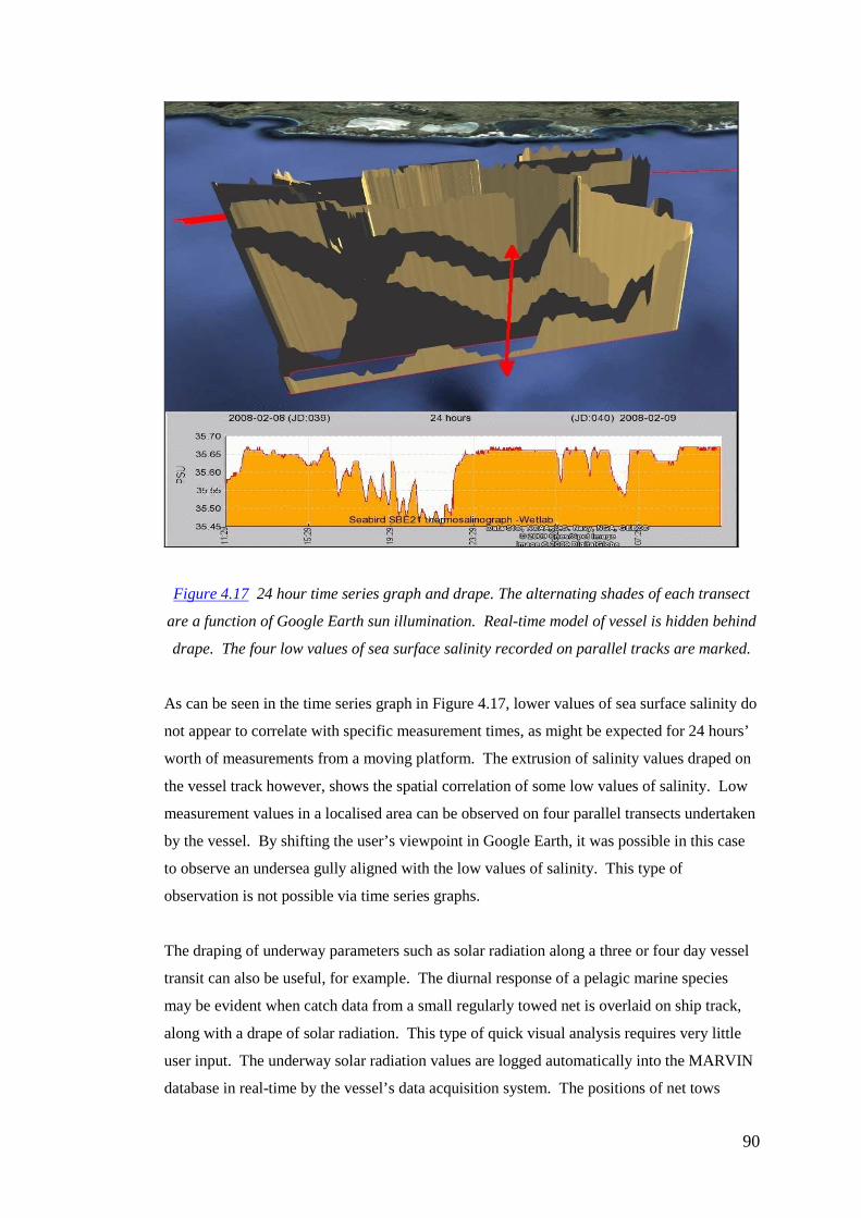
90
Figure 4.17 24 hour time series graph and drape. The alternating shades of each transect
are a function of Google Earth sun illumination. Real-time model of vessel is hidden behind
drape. The four low values of sea surface salinity recorded on parallel tracks are marked.
As can be seen in the time series graph in Figure 4.17, lower values of sea surface salinity do
not appear to correlate with specific measurement times, as might be expected for 24 hours’
worth of measurements from a moving platform. The extrusion of salinity values draped on
the vessel track however, shows the spatial correlation of some low values of salinity. Low
measurement values in a localised area can be observed on four parallel transects undertaken
by the vessel. By shifting the user’s viewpoint in Google Earth, it was possible in this case
to observe an undersea gully aligned with the low values of salinity. This type of
observation is not possible via time series graphs.
The draping of underway parameters such as solar radiation along a three or four day vessel
transit can also be useful, for example. The diurnal response of a pelagic marine species
may be evident when catch data from a small regularly towed net is overlaid on ship track,
along with a drape of solar radiation. This type of quick visual analysis requires very little
user input. The underway solar radiation values are logged automatically into the MARVIN
database in real-time by the vessel’s data acquisition system. The positions of net tows

91
would be easily entered as waypoints into MARVIN as part of standard log keeping practice.
The type or amount of catch from each net tow can be used to set the symbology used to
display waypoints in MARVIN Google Earth clients, as is illustrated in following sections.
This quick method allows the correlation of catch amount or type, versus light intensity to be
assessed via a visual method.
4.8 MARVIN scenarios
This section briefly presents scenarios which illustrate the use of MARVIN during a marine
research voyage. The scenarios presented are typical of the many quick and not so quick,
spatial data analysis tasks, which may be undertaken during a research voyage.
Whilst the scenarios described are straightforward, it should be appreciated that as MARVIN
is a multi-user tool, the simple tasks described within the scenarios could be concurrently
undertaken by multiple users via multiple Google Earth clients. All users would
concurrently access the same real-time spatio-temporal datasets, using the same interface on
their computers (Google Earth), which symbolised the datasets using the same colours and
icons.
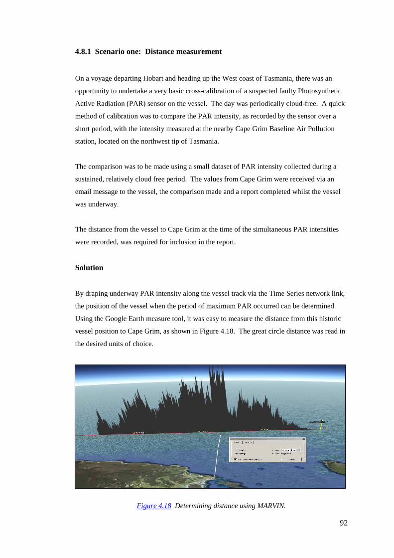
92
4.8.1 Scenario one: Distance measurement
On a voyage departing Hobart and heading up the West coast of Tasmania, there was an
opportunity to undertake a very basic cross-calibration of a suspected faulty Photosynthetic
Active Radiation (PAR) sensor on the vessel. The day was periodically cloud-free. A quick
method of calibration was to compare the PAR intensity, as recorded by the sensor over a
short period, with the intensity measured at the nearby Cape Grim Baseline Air Pollution
station, located on the northwest tip of Tasmania.
The comparison was to be made using a small dataset of PAR intensity collected during a
sustained, relatively cloud free period. The values from Cape Grim were received via an
email message to the vessel, the comparison made and a report completed whilst the vessel
was underway.
The distance from the vessel to Cape Grim at the time of the simultaneous PAR intensities
were recorded, was required for inclusion in the report.
Solution
By draping underway PAR intensity along the vessel track via the Time Series network link,
the position of the vessel when the period of maximum PAR occurred can be determined.
Using the Google Earth measure tool, it was easy to measure the distance from this historic
vessel position to Cape Grim, as shown in Figure 4.18. The great circle distance was read in
the desired units of choice.
Figure 4.18 Determining distance using MARVIN.
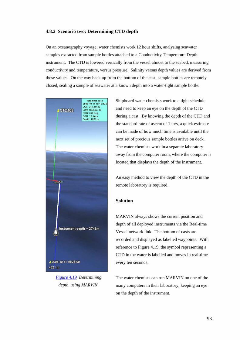
93
4.8.2 Scenario two: Determining CTD depth
On an oceanography voyage, water chemists work 12 hour shifts, analysing seawater
samples extracted from sample bottles attached to a Conductivity Temperature Depth
instrument. The CTD is lowered vertically from the vessel almost to the seabed, measuring
conductivity and temperature, versus pressure. Salinity versus depth values are derived from
these values. On the way back up from the bottom of the cast, sample bottles are remotely
closed, sealing a sample of seawater at a known depth into a water-tight sample bottle.
Figure 4.19 Determining
depth using MARVIN.
Shipboard water chemists work to a tight schedule
and need to keep an eye on the depth of the CTD
during a cast. By knowing the depth of the CTD and
the standard rate of ascent of 1 m/s, a quick estimate
can be made of how much time is available until the
next set of precious sample bottles arrive on deck.
The water chemists work in a separate laboratory
away from the computer room, where the computer is
located that displays the depth of the instrument.
An easy method to view the depth of the CTD in the
remote laboratory is required.
Solution
MARVIN always shows the current position and
depth of all deployed instruments via the Real-time
Vessel network link. The bottom of casts are
recorded and displayed as labelled waypoints. With
reference to Figure 4.19, the symbol representing a
CTD in the water is labelled and moves in real-time
every ten seconds.
The water chemists can run MARVIN on one of the
many computers in their laboratory, keeping an eye
on the depth of the instrument.
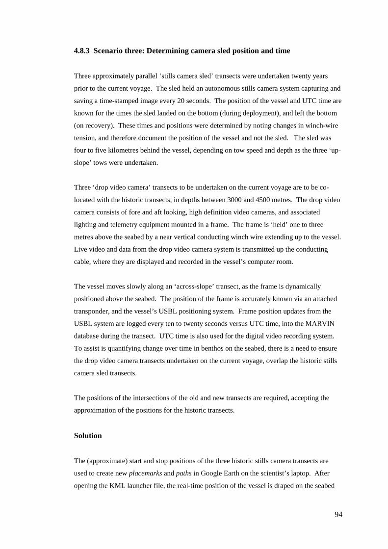
94
4.8.3 Scenario three: Determining camera sled position and time
Three approximately parallel ‘stills camera sled’ transects were undertaken twenty years
prior to the current voyage. The sled held an autonomous stills camera system capturing and
saving a time-stamped image every 20 seconds. The position of the vessel and UTC time are
known for the times the sled landed on the bottom (during deployment), and left the bottom
(on recovery). These times and positions were determined by noting changes in winch-wire
tension, and therefore document the position of the vessel and not the sled. The sled was
four to five kilometres behind the vessel, depending on tow speed and depth as the three ‘up-
slope’ tows were undertaken.
Three ‘drop video camera’ transects to be undertaken on the current voyage are to be co-
located with the historic transects, in depths between 3000 and 4500 metres. The drop video
camera consists of fore and aft looking, high definition video cameras, and associated
lighting and telemetry equipment mounted in a frame. The frame is ‘held’ one to three
metres above the seabed by a near vertical conducting winch wire extending up to the vessel.
Live video and data from the drop video camera system is transmitted up the conducting
cable, where they are displayed and recorded in the vessel’s computer room.
The vessel moves slowly along an ‘across-slope’ transect, as the frame is dynamically
positioned above the seabed. The position of the frame is accurately known via an attached
transponder, and the vessel’s USBL positioning system. Frame position updates from the
USBL system are logged every ten to twenty seconds versus UTC time, into the MARVIN
database during the transect. UTC time is also used for the digital video recording system.
To assist is quantifying change over time in benthos on the seabed, there is a need to ensure
the drop video camera transects undertaken on the current voyage, overlap the historic stills
camera sled transects.
The positions of the intersections of the old and new transects are required, accepting the
approximation of the positions for the historic transects.
Solution
The (approximate) start and stop positions of the three historic stills camera transects are
used to create new placemarks and paths in Google Earth on the scientist’s laptop. After
opening the KML launcher file, the real-time position of the vessel is draped on the seabed
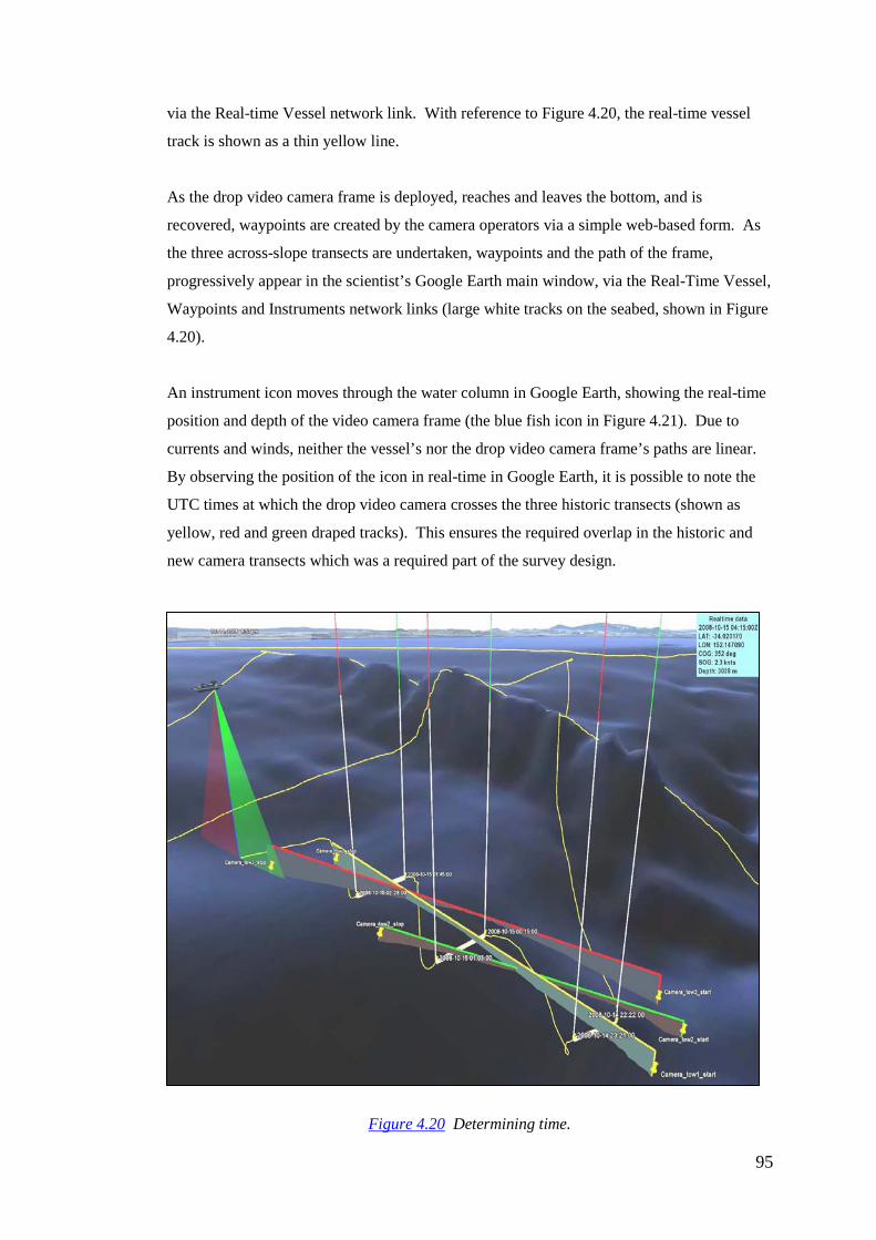
95
via the Real-time Vessel network link. With reference to Figure 4.20, the real-time vessel
track is shown as a thin yellow line.
As the drop video camera frame is deployed, reaches and leaves the bottom, and is
recovered, waypoints are created by the camera operators via a simple web-based form. As
the three across-slope transects are undertaken, waypoints and the path of the frame,
progressively appear in the scientist’s Google Earth main window, via the Real-Time Vessel,
Waypoints and Instruments network links (large white tracks on the seabed, shown in Figure
4.20).
An instrument icon moves through the water column in Google Earth, showing the real-time
position and depth of the video camera frame (the blue fish icon in Figure 4.21). Due to
currents and winds, neither the vessel’s nor the drop video camera frame’s paths are linear.
By observing the position of the icon in real-time in Google Earth, it is possible to note the
UTC times at which the drop video camera crosses the three historic transects (shown as
yellow, red and green draped tracks). This ensures the required overlap in the historic and
new camera transects which was a required part of the survey design.
Figure 4.20 Determining time.

96
If the position and time of the crossing(s) of the two sets of transects is not noted during the
deployment, the Instruments network link can be used after instrument recovery to determine
these values. In conjunction with the time control tool, the position of the drop video
camera frame, shown by the historic instrument icon (the blue fish icon in Figure 4.21),
moves in 3D space, as time is varied. The UTC time at the crossover point can be noted,
allowing a later manual search for matching imagery, from both the historic and new
transects.
Figure 4.21 Small-scale view of a single drop video camera transect and
two historic stills camera sled transects.
Figure 4.21 shows a small-scale view of a single drop video camera transect (large white
line) and the path of two historic stills camera sled transects (green and yellow). As the time
control tool is moved backwards and forwards through time, the position of the fish icon
representing the drop video camera frame changes. Its position varies back and forth along
the 3D underwater path (thick white line), according to the 4D spatio-temporal data,
recorded in the MARVIN database. To produce Figure 4.21, the time was adjusted until the
icon was positioned at the intersection of the new and historic transects. The time and depth
can be seen next to the icon (3935 metres 00:48:10 15th October 2008).
Of note in Figure 4.21 is the display of a red drape showing vessel track. A gap can be seen
between the thick white line, showing the video camera frame’s 3D path, and the base of the
red drape, representing the 2D track of the vessel. This gap represents the horizontal offset
between the vessel and the camera frame, caused by vessel speed, wind, water currents, and
tow cable and frame hydrodynamics.

97
As MARVIN updates the view shown in Figure 4.21 in real-time, the offset can be measured
in real-time using the Google Earth measure tool. If there is a desire to closely maintain the
course of the camera frame rather than the course of the vessel, along a pre-defined transect,
action can be taken if the gap is larger than desired. Bridge crew can be asked to gradually
offset the vessel position from the planned transect by the same amount, to reposition the
video camera frame back towards the path of the original planned transect.
4.8.4 Scenario four: Contaminated site
A component of a marine research voyage is to determine sediment contamination down-
slope from the approximate position of a disused munitions dump. The Australian Navy has
not used the site for fifty years and the exact coordinates of the dumpsite have been lost. A
survey was undertaken twenty years prior to the current voyage, determining sediment
contamination using dredges and coring. A paper navigation chart exists (in fathoms) from
the original survey, which shows approximately the boundaries for regions of classified
contaminate levels. Whilst the sample site contaminate levels are known, the sample site
locations have been lost.
A Multi-Beam Echo-Sounder survey is undertaken of the area to map the seabed topography
around the assumed site of the dump. The spacing of survey transects is determined by the
width of the Multi-Beam Echo-Sounder swath, which is dependent on operating depth.
Vertical sediment grabs are to be completed as the vessel stops every hour along the path of
each parallel transect.
In this scenario, it is important to ensure the new survey is being undertaken in the correct
location before the vessel leaves the region. This means there is a requirement at sea to
undertake a ‘first-pass’ comparison of contaminate levels found during the original survey,
with those found during the current voyage. The accuracy of this comparison is limited by
the analysis techniques available onboard. The techniques are sufficiently sensitive
however, to determine whether current contaminate levels measured are above regional
background levels.
A quick visual technique is required to compare present-day contaminate levels determined
by on-board analyses, with historic measurements, to ensure the correct location has been
chosen for the new survey.

98
Solution
As the only data from the original survey are boundaries on a paper chart, the paper chart (in
fathoms) is scanned and added to Google Earth as an image overlay. Boundaries are
digitised on-screen to create polygons representing contaminate levels. The Electronic
Charting and Display Information System (ECDIS) on the bridge uses Electronic Navigation
Charts (ENC) in metres, so the pre-metric chart overlay is removed from Google Earth,
before a metric version is added, to prevent possible confusion.
During the voyage, a waypoint is created each time a sediment grab is undertaken via simple
web-based forms. The forms allow for the entry of a comment and the selection of a symbol
for use in MARVIN. These equipment waypoints appear on all computers accessing
MARVIN as sediment grabs are completed. The vessel track and vessel real-time position
likewise appear, enabling scientific personnel an overview of the position of the vessel on
their laptop computers, from convenient locations.
As onboard analyses of sediment contaminate levels are completed for each sediment grab,
web-based forms are used to assign a symbol and classification (A,B,C and so on), to the
waypoint in the MARVIN database, based on the level of contaminates found. After
sufficient samples and analyses have been completed, the correlation between original and
new contaminate datasets can be assessed. Through visual interpretation of the waypoint
symbols and the underlying choropleth map showing historic contaminate level, a simple
analysis of the evolving dataset can be undertaken. Figure 4.22 shows the scenario survey
area, as is seen in real-time on all MARVIN clients.
Figure 4.22 shows reasonable spatial correlation between the two contaminate datasets. The
classifications applied via the web-based waypoint entry forms enables Google Earth to
show differing symbols for each range of contaminate level (A = high and B= medium,
present day contaminate levels, which spatially correlate with red=high and green=medium
historic contaminate levels and so forth).
With this knowledge, the survey can continue as planned as there is confidence that the
current survey is being conducted over the dump site. Shore-based analyses will enable an
analytical comparison between the original and present day contaminate levels.
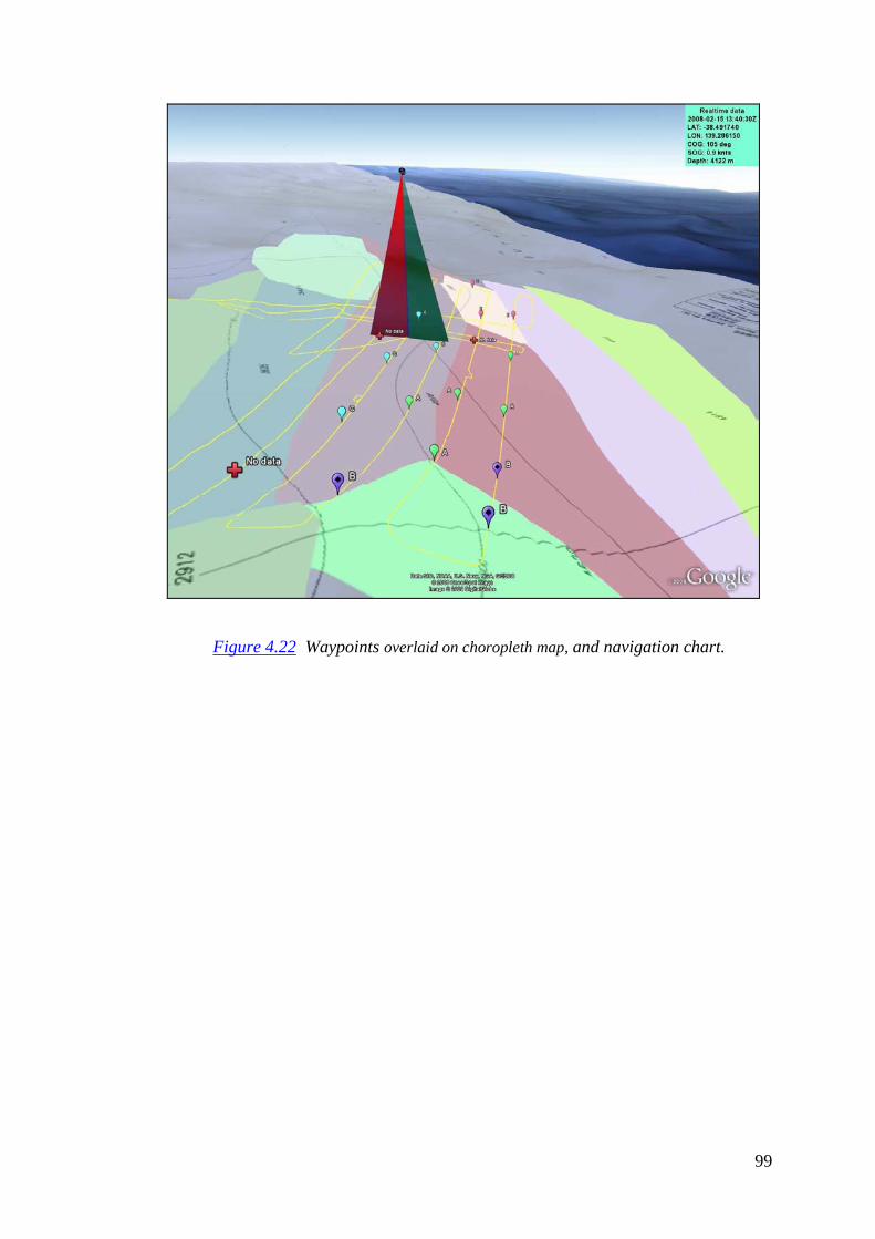
99
Figure 4.22 Waypoints overlaid on choropleth map, and navigation chart.
100
4.9 Summary
This chapter provided a brief overview of the use and capabilities of MARVIN. Interested
readers are again referred to the downloadable figures and KML files, which allow a more
interactive demonstration of the results of this research.
The simple scenarios described have shown four typical applications for MARVIN during a
marine research voyage. It should be appreciated that MARVIN was intended to be a real-
time and multi-user system, allowing simple and quick visualisation of real-time datasets. It
is not intended to be a replacement for a desktop GIS.
A desktop GIS would to able to undertake some of the tasks described in the scenarios, as
well as a vast array of other simple and more advanced, operations and analyses, which
would be useful at sea. Reader (2009) however discusses the limits of both 3D and 4D
dataset support in current GIS software “… exists a need to develop appropriate data
structures and data models for the handling of 3-D and temporal data within GIS”.
Malzone et al. (2009) are equally critical of attempting to coerce current GIS software into
efficiently undertaking analyses which invlove the third and forth dimensions. Given the 4D
environment that data is collected in during a marine research voyage, robust 4D methods of
visualisation and analysis are required.
Hatcher et al. (2006) states “The GIS can be a powerful tool for all phases of an
oceanographic cruise, but with this power comes a significant level of complexity and a non-
trivial learning curve”. The level of complexity of the installation of GIS software, support
for security of datasets, and need for good ‘data housekeeping’, increases markedly if
multiple GIS clients were used for simple 3D and (where possible) 4D analyses, to replicate
the multi-user functionality provided by MARVIN.
All of the scenarios provided are independent of software installed on user’s computers apart
from Google Earth. The screen captures of the Google Earth main window shown in the
figures in the scenarios show a view of MARVIN as would be accessible from as many
computers as required. Very little user entry and no detailed GIS or mapping knowledge
were required during the scenarios.

101
Chapter 5 Discussion
This chapter discusses the achievements of the research undertaken and explains the
significance of the results presented in the previous chapter. The abilities of MARVIN, as an
indicator of the suitability of the combination of a spatio-temporal DBMS and KML, are
compared briefly with other software techniques commonly used during marine research
voyages.
Figure 5.1 Screen capture of MARVIN, showing complete Google Earth GUI.
Figure 5.1 shows a screen capture from a typical MARVIN session using Google Earth.
This figure shows the majority of the MARVIN layers as provided by the six network links
controlled by the user. This figure is in comparison to the screen captures shown in all
figures in prior chapters, which were created with the majority of layers disabled for clarity.
With reference to Figure 5.1, the Southern Surveyor has departed Hobart for Voyage One of
2008 (SS2008_V01). She is traversing down the continental slope south of Tasmania at a
speed of 10.9 knots in a southwesterly direction. Water depth is 790 metres at 19:54:50 on
the 11th January 2008 UTC (Julian Jay JD11). Waypoint CTD150 is approximately 15
kilometres away from the (then) current vessel position. The pop-up balloon for the
102
waypoint shows the instrument type and its planned location. The historic (red) vessel
model is positioned at the historic epoch of 19:12:20 UTC on the same day in 306 metres of
water, controlled by the user via the Google Earth time control tool shown in the top left
corner. A time series graph of Photosynthetic Active Radiation (PAR) for the 24 hour period
prior to the (then) current time is shown. The start of data acquisition at approximately 03:50
UTC correlates with high PAR values. As can be seen in the time series graph, data logging
of underway parameters on the voyage commenced just prior to 2pm AEDT, on a relatively
cloud free January Hobart day.
The Google Earth side bar shown is Figure 5.1 shows the names of all equipment
deployment locations (as waypoints), which are planned or have already been undertaken.
The side bar also shows that display of the large vessel model and three hourly waypoints
has been enabled, and that the bottom planimetric chart covers a 40km x 40km geographic
area. The bottom planimetric chart also shows the vessel track as a green or brown line,
where the transition between the colours shows the last even three hour transition (0000,
0300, 0600 UTC and so on), which in this case was 1800 UTC. These transitions correlate
with the waypoints showing the position of the three hourly observations.
5.1 Introduction
With reference to the previous chapter, MARVIN was found to be very easy to use. It was
found to be an intuitive multi-user system, which allowed the visualisation of both real-time
and historic, spatio-temporal data. MARVIN allowed a true 4D view of the real-time data it
was assessed with.
The use of a Virtual Globe (Google Earth in this instance) allowed the user’s view elevation
to be changed rapidly and easily. The ability to view spatial data at a very wide variety of
scales, controlled by viewpoint elevation, is a unique requirement of many marine research
programs undertaken onboard blue water research vessels. A voyage may start at an
Australian port and finish at a foreign port. Instruments may be towed behind the vessel for
many days recording plankton concentrations, or dragged across the seabed for a few
minutes collecting rock samples. The use of a Virtual Globe browser allowed view elevation
to be quickly varied from a voyage based view, covering tens of degrees of longitude or
latitude, to a two nautical mile view showing the profile of a shallow water dredge, for
example.

103
View direction and angle could also be varied very quickly. This enabled the use of both
near-planimetric views (on a globe) for viewing datasets such as vessel track and waypoints,
as well as low angle oblique views for use with datasets such as the 4D paths of mid-water
nets or towed camera systems.
The view scale, direction and angle were easily controllable by MARVIN users using the
computer mouse. The actual on-screen scale of the view was of less importance than the
ability to produce a 4D view of 4D datasets from a suitable user determined view direction,
angle and elevation. Google Earth does not provide the user with a numeric scale value as it
is would be meaningless for any views apart from those perpendicular to the Earth’s surface
(normal) and at low altitudes.
The inability to enable and disable layers via the Google Earth side bar was invaluable. By
grouping common functions into six separate network links, it was possible to very easily
disable a group of layers that were not required. For instance, planimetric maps or time-
series graphs and drapes could be removed from the Google Earth main display, by disabling
the Time Series or Real-time Charts network links respectively. KML supports both tick
boxes and radio buttons for enabling and disabling layers. Radio buttons are used when
there is a need to enforce the enabling of only a single layer, within a directory of layers.
This very useful KML ability was used in MARVIN to enable the user to select the type of
planimetric charts to display in the upper and lower positions in the Google Earth main
window.
The use of KML as the method for streaming both spatio-temporal data and symbology to
Google Earth worked well. It enabled the use of common symbology on all clients accessing
MARVIN. The requirement for a system such as MARVIN to support multiple users who
have little time at sea to learn new software packages, meant consistency in symbology was
important.
The accommodation of elevation data in KML and therefore MARVIN was robust. The
provision in KML to accommodate positive and negative, relative and absolute, sea surface
and seabed referenced elevation values was invaluable. By using the sea surface as the
vertical datum, depth values in the KML datastream are relative to the vessel (which is
positioned on the sea surface). This method accommodates depths derived from a vessel
mounted positioning system. Likewise, when a dredge or net was known to be positioned on

104
the seabed via a measurement of trawl wire tension, it was possible to lock the dredge
position to the Google supplied DEM by using the seabed as the vertical datum.
This enabled the track of an instrument dragged across the seabed to correctly overlay the
Google supplied DEM. Google Earth limitations for accommodating negative elevation
values (depths) as discussed by Dunne et al. (2006) and Blower at al. (2006) no longer exist
for versions greater than v5.0. Google Earth fully supports all methods of specifying
positive and negative elevation values, as defined in the OGC KML 2.2 Reference – an OGC
Best Practice (Open Geospatial Consortium Inc., 2007)
The time component of spatio-temporal data in the MARVIN database was accommodated
by the time stamping functions of the KML language. The positions versus times of objects
such as vessel models, were able to be embedded in the KML datastream. This enabled a
holistic view of all spatio-temporal data in the MARVIN database to be created for a user
specified historic epoch. Answers such as “What direction and speed was the vessel doing
when the trawl net was at a particular depth?” were able to be answered via an intuitive and
graphical technique.
MARVIN was tested for use with the uSer-Friendly [sic] Desktop Internet Gis application
(uDig). Figure 5.2 shows the uDig Java application accessing spatio-temporal data stored in
the MARVIN database. uDig is a popular limited feature open-source desktop GIS
application which supports direct access to a PostgreSQL database for accessing spatial data
stored as OGC geometries. As previously discussed, there was a need to accommodate
desktop GIS software to access some of the useful functionality it can provide at sea, when
building MARVIN.
The yellow vessel tracks shown in Figure 5.2 show a subset of the 1.9 million vessel
positions stored in the underway_navigation table of the MARVIN database. The real-time
data uDig was accessing was the same spatio-temporal data MARVIN used as the basis for
generating KML datastreams for Google Earth clients.

105
Figure 5.2 User-friendly Desktop Internet GIS (uDig) screen capture,
showing direct access to MARVIN’s database.
Additionally, Figure 5.2 also shows uDig accessing the illuminated DEM GEOTIFF image
used by MARVIN as the background image of the upper planimetric chart embedded in the
main window of Google Earth clients. uDig supports WMS for accessing raster maps from
remote computers. Access to the DEM was provided via MapServer running as a CGI
program on the MARVIN server, serving WMS requests from remote clients (uDig in this
example).
The ability to view MARVIN’s dynamically created spatio-temporal datasets simultaneously
by a Virtual Globe such as Google Earth and by a desktop GIS application such as uDig, is
possible through the use of the PostgreSQL database. This single source of all real-time
spatio-temporal data visualised by MARVIN clients and GIS applications, enables the
advantages of both data visualisation methods to be gained. The most suitable mapping,
visualisation or spatio-temporal analysis techniques can all be used in real-time, by multiple
users during a research voyage, accessing the same dynamic dataset. The technique to use
would typically be dictated by time, user ability, software availability and type of task to be
undertaken.
As has been discussed previously, the ability to use a desktop GIS with the MARVIN DBMS
is advantageous when the printing of a cartographic product such as a paper chart is required.
A full featured desktop GIS package, as opposed to uDig, generally enables an experienced

106
user to produce a paper chart to a high cartographic standard. These abilities complement
the abilities of a Virtual Browser accessing MARVIN, by allowing both a 4D computer
display view and a 2D paper chart of the dataset. The limitations of using a package such as
uDig or any desktop GIS for real-time 4D multi-user spatio-temporal operations or analyses
however, are discussed in the next section.
With reference to the simple scenarios described in the previous chapter, which briefly
illustrated typical uses for MARVIN during a marine research voyage, it is possible to
compare MARVIN with other existing software based spatial analysis techniques.
Comparisons in the next sections have been limited to desktop GIS, and advanced 3D (and
4D) visualisation software packages.
5.2 MARVIN versus GIS software
As previously outlined, the use of desktop GIS during voyages in support of marine research,
is much less common than its use in supporting marine or terrestrial research undertaken in
laboratories and offices. Desktop GIS is often seen as being too complicated, too large, or
too slow for use as a robust tool to be used at sea. In particular, commonly available open-
source desktop GIS software packages do not lend themselves to use by the inexperienced at
sea, due to the lack of examples and documentation provided.
Reasons for these opinions include the reality of the steep learning curve new users of
comprehensive GIS software packages face, and the invariable time constraints scientists and
support staff face at sea. This was a consistent theme in much of the literature reviewed,
including Donald (2005) and Hatcher et al. (2006).
Nonetheless, individual researchers and individual research groups do currently use desktop
GIS software during research voyages. General purpose mapping tasks and complicated
spatial operations can be very effectively undertaken if the user is proficient in the use of the
software. The use of GIS software during a research voyage is a natural extension to its use
in the office. Layers of information, such as vessel track and waypoint locations, can be
added in near real-time or real-time (as per the uDig example illustrated above). Catch data
from fishing trawls or dredges can be quickly collated and added as another layer in the GIS
for example. The detail achievable is generally limited by time, expertise and on-board
equipment.

107
However, standard desktop GIS software does not readily accommodate real-time data and
data with elevations and data with time components. With reference to the simple uDig
example discussed above, it is not possible to view the MARVIN sourced datasets in
anything other than a planimetric view, and the accommodation of advanced symbology is
limited.
The techniques employed ashore, in an attempt to accommodate these deficiencies, can also
be used at sea. Depth and time values can be associated with the position of an object, via
attribute values, rather than treating depth and time as the third and forth dimensions of a
spatio-temporal data. Dynamic datasets, such as shiptrack and waypoints, can be sourced
from a constantly updated database of positions and attributes (such as MARVIN’s DBMS).
More advanced techniques exist, such as building a highly customised tool using commercial
desktop GIS software in conjunction with a GIS vendor’s supported programming language.
CASINO+ from IFREMER (Institut français de recherche pour l'exploitation de la mer) is
based on this technique, using ArcMap 9.3 from ESRI. These advanced techniques can
support real-time data, allowing a true up-to-date 2D desktop GIS, for single user use.
The techniques described are all based on accommodating current limitations in desktop GIS
software. Techniques such as these are widely employed, and in some circumstances, can
allow an open-source or commercial GIS, modified slightly or heavily customised, to offer
limited support for real-time spatio-temporal datasets.
Whilst these techniques can offer functionality, they also add a great deal of complexity.
They often require the user to be proficient in the use of the specific GIS software package,
as well as the specific tools built to enhance the GIS, allowing the accommodation of real-
time datasets. The install base for these tools is extremely small as even the largest of
marine research organisations does not have more than a handful of vessels. The majority of
scientists on many research voyages where such tools are available will not have experience
with the GIS software or the specific customisations employed. These solutions can never
offer a robust real-time and 4D and multi-user solution.
For instance, the tasks outlined in the four scenarios described in the previous chapter, could
be undertaken at sea using a commercial or open-source GIS. A commercial GIS package
such as ArcMap could be used with datasets extracted from the MARVIN DBMS or from
text files collected by a vessel’s data acquisition system. Techniques to accommodate depth
108
and time such as those described above could be employed, and these and many other simple
analyses completed.
In practice however, due to the need to: constantly refresh the ever changing datasets (if real-
time access to the MARVIN database is not possible); be familiar with the GIS software; and
be proficient in a language such as SQL, it is unlikely to be a robust solution. This approach
also limits the user to undertaking simple mapping or visualising tasks on a computer with a
full commercial GIS software package installed. As a commercial GIS software package is
unlikely to be available on more than two or three computers on a large research vessel, this
solution provides neither a robust nor simple multi-user solution.
5.3 MARVIN versus specialised 3D and 4D modelling software
Specialised software packages such as Fledermaus and Eonfusion offer functionality similar
to MARVIN. The use of these advanced spatio-temporal data visualisation packages is
commonplace in fields such as hydroacoustics and benthic habitat mapping, where large 3D
and 4D datasets need to be visualised and used in analyses.
With reference again to the scenarios described in the previous chapter, both Fledermaus and
Eonfusion could be used to undertake these tasks. Eonfusion’s (unique) ability to
accommodate four dimensional datasets is of particular relevance to some of the scenarios
described. Many simple and complex visualisations and analyses could be undertaken
during a marine research voyage with these advanced packages.
Whilst these software packages overcome many of the limitations of attempting to use
desktop GIS software with 4D datasets, their use comes at a cost. The complexity of the
software, and to a lesser extent the financial cost of purchase, makes the use of these
packages to provide robust multi-user functionality (similar to MARVIN) highly unlikely.
These packages are not intended to be used in a multi-user environment with centralised
dynamic datasets, and it is unreasonable to expect that licenses would be available for more
than one or two computers on a typical research vessel. This is not to say that these very
powerful software tools do not have a place at sea in supporting specific research programs
where expertise is available onboard to utilise their full functionality.

109
Chapter 6 Conclusion
The combination of a DataBase Management System and the Keyhole Markup Language for
the storage and streaming of real-time spatio-temporal datasets was found to offer a robust
solution to the question of “How to visualise real-time spatio-temporal datasets at sea, in a
multi-user environment?”.
A server-based tool called MARVIN was built using an open-source spatio-temporal DBMS,
and KML. A DBMS was used to store real-time spatio-temporal data, accommodating both
the 3D position and time of the data. The support of OGC geometries by the DBMS made
possible many types of necessary spatio-temporal GIS operations, such as ‘on-the-fly’ re-
projection and great circle distance calculations. The spatial operators of the SQL language
in conjunction with the PHP programming language enabled spatial operations to be
undertaken wholly within the DBMS.
Spatio-temporal datasets were streamed to Virtual Globe browsers using KML. The
Keyhole Markup Language was able to effectively encapsulate both the spatial and temporal
components of geographic objects, which were subsequently visualised in 4D in Virtual
Globe browsers.
The aims and objectives of this research as outlined in Chapter One were met as detailed
below.
• A review of existing methods and tools allowing web-based or multi-user,
exploration and mapping was undertaken. Both mature and developing technologies
were reviewed.
• MARVIN was developed to allow the efficient storage and visualisation of typical
real-time spatio-temporal datasets collected at sea during a marine research voyage.
MARVIN was found to allow intuitive 4D exploration of real-time datasets via a
Google Earth Virtual Globe Browser.
• The software components of MARVIN were evaluated and limitations discussed. In
particular, the suitability of a DBMS in conjunction with KML for allowing multi-
user exploration of real-time spatio-temporal datasets was investigated.

110
• The functionality of MARVIN was illustrated via a series of simple but realistic case
studies, using historical empirical datasets collected at sea. Datasets typical of those
collected and analysed at sea were also simulated to allow realistic testing of
MARVIN’s 4D capabilities.
By meeting the aims and objectives of this study, MARVIN was shown to fill a gap in the
functionalities which had been identified in existing software tools. No solution existed
which permitted the multi-user exploration of real-time spatio-temporal data.
A summary of the major strengths and challenges, and suggestions for future work are
detailed in the following sections.
6.1 Major strengths
True 4D capabilities
By using KML for the encapsulation of spatio-temporal data, MARVIN enabled the visual
exploration of 4D datasets using Virtual Globe browsers. Both the spatial and temporal
attributes of the data stored in the real-time spatio-temporal database were accommodated.
MARVIN users were able to move through space and time, to a desired location or epoch.
Real-time capabilities
By using a DBMS to fulfill all data storage requirements, real-time data were able to be
accommodated by MARVIN. The use of a DBMS permitted the simultaneous creation,
storage, retrieval and manipulation of spatio-temporal data by multiple processes and users.
The DBMS ensured a high level of data security, integrity and reliability.
111
Multi user capabilities
The adoption of a true client-server model for MARVIN enabled multi-user support. The
combination of a DBMS, KML and associated server-side processes, created a robust
framework onto which MARVIN could be built. Multiple users could simultaneously and
independently move through space and time, exploring the same real-time spatio-temporal
dataset from different viewpoints in space, at different epochs in time.
6.2 Major challenges
The reliance on Network Links limited the use of the Virtual Globe browsers usable with
MARVIN. No other Virtual Globe browser currently supports Network Links as defined in
the OGC KML v2.2 standard apart from Google Earth.
The Google Earth sea surface is a rippled illuminated animation. The animation works well
for general use and can be enabled and disabled in the Google Earth browser as required.
There is currently no transparency percentage control in version 5.0, and the translucent
surface automatically and progressively, becomes opaque when viewed from low view
angles. The elevation of the sea surface is an important vertical datum when visualising
objects above, on, and below the sea surface and its automatic opacity in Google Earth based
on user view angle is problematic. 3D paths of underwater equipment can dissapear under
the opaque sea surface when a user changes their view position or angle for a better look.
The creation of identical multiple temporary images by MARVIN for use by multiple Virtual
Globe clients lacked scalability. Whilst functional, the disk and network load on the small
MARVIN server was excessive when more than two or three Virtual Globes clients were
connected. For scalability, it is feasible in future revisions of MARVIN to repeatedly
generate one set of shared real-time images which could be concurrently accessed by all
Virtual Globe clients. The use of WFS to provide access to near real-time 3D spatial
datasets in conjunction with real-time 4D spatio-temporal datasets provided via KML may
also offer performance advantages.
112
6.3 Future Work
The combination of very mature DBMS technology, with widely supported but evolving
OGC standards such as KML, means the research detailed in this thesis will date. The future
evolution of WMS, WFS, KML and other developing OGC standards means the use of these
standards to achieve design goals similar to MARVIN needs further research.
The continued release of commercial, open-source and royalty free versions of Virtual Globe
browsers is likely. As many browsers will no doubt be usable with a system such as
MARVIN, the abilities of new software packages should be investigated. The use of APIs
which allow Virtual Globes to be accessible via web browsers or standalone applications,
may overcome some of the limitations of currently available Virtual Globes, such as the
inability to replace sections of the Google supplied DEM.
The improving support of Virtual Globes in commercial desktop GIS software should be
researched. If the power of desktop GIS software is melded fully with the visualisation
abilities of a Virtual Globe, there is the possibility that this combination of technologies may
offer many of the 4D advantages of MARVIN along with the analysis power of desktop GIS
software.
Virtual Globes have been used in support of many scientific applications during their short
history. The continual improvement of the functionality of Virtual Globes makes their use at
sea for supporting marine research a robust solution. The demonstration in this thesis of
their functionality in conjunction with a spatio-temporal DBMS and KML, builds faith in
this evolving collection of technologies.
“Don't build a new ship out of old wood”
Chinese Proverb
113
References
Apache Software Foundation. "HTTP server Project." Retrieved 2nd June, 2009, from
http://www.apache.org
Bacharach, S. (2009). "Review: OpenGIS Web Map Tiling Service (WMTS) Interface
Specification." Retrieved 12th September, 2009, from http://xml.coverpages.org/OGC-
WMTS-Candidate.html
Blower, J., Bretherton, D., Haines, K., Liu, C. and Santokhee, A. (2006). "Exploring Large
Marine Datasets Using an Interactive Website and Google Earth." American Geopysical
Union - Eos 87(52), from
http://www.resc.reading.ac.uk/publications/Blower_AGUFall06.ppt
Burrough, P. A. and Mcdonnell, A. (1998). Principles of Geographical Information Systems.
Oxford, Oxford Press
Cerami, E. (2002). Web Services Essentials. SF, O'Reilly
Di Felice, P. and Pomante, L. (2006). Integration of Spatial Data Types and Operators into
Relational DBMSs: A Survey. IADIS International Conference Applied Computing 2006,
from http://www.iadis.net/dl/final_uploads/200601P005.pdf
Donald, J. (2005). Voting with Your Hands: GIS and Experiential Learning. 2005 ESRI
Education User Conference, San Diego, California, ESRI, from
http://proceedings.esri.com/library/userconf/educ05/papers/pap1714.pdf
Dunne, D. and Sutton, G. (2006). "3D Web-mapping - Integrating Marine Data into Google
Earth." Hydro International Journal 10(7), from http://www.hydro-
international.com/issues/articles/id650-D_Webmapping.html
Elissalde, P. (2007). "2D/3D Wep-mapping - Web Visualisation Coastal Orthophotos."
Hydro International Journal 11(3), from http://www.hydro-
international.com/issues/articles/id756-DD_Webmapping.html

114
Elvidge, C. D. and Tuttle, B. T. (2008). How Virtual Globes are Revolutionizing Earth
Observation Data Acess and Integration. ISPRS Congress Beijing 2008, Beijing,
International Society for Photogrammetry and Remote Sensing, from
http://www.isprs.org/congresses/beijing2008/proceedings/6a_pdf/4_WG-VI-4/01.pdf
Environmental Systems Research Institute. (1992). Understanding GIS: The Arc/Info
Method, Lesson 1: Why GIS. Redlands, CA, ESRI
Environmental Systems Research Institute. (1998). Spatial Data Warehousing. An ESRI
White Paper. ESRI. Redlands
Environmental Systems Research Institute. (2009). "Understanding ESRI's Free "Explorer"
Applications." Retrieved 3rd May, 2009, from
http://www.esri.com/software/arcexplorer/explorer.html
Geoscience Australia. "OGC Web Map Services (WMS) details, Geoscience Australia."
Retrieved 12th July, 2009, from http://www.ga.gov.au/map/broker/wms_info.php
Geoserver. "GeoServer Documentation." Retrieved 1st May, 2009, from
http://docs.geoserver.org/1.7.x/en/user
Geospatial Dataservice Centre. (2009). "WMS Client Software." Retrieved 4th June, 2009,
from http://gdsc.nlr.nl/gdsc/information/ogc/wms/client_software
Groff, J. R. and Weinberg, P. N. (2003). SQL. The Complete Reference. NY, Osborne.
Guting, R. H. (1994). "An Introduction to Spatial Database Systems." Very Large Database
Journal 3(4), from
http://www.cise.ufl.edu/~mschneid/Research/thesis_papers/Gue94VLDBJ.pdf
Hatcher, G. A. and Maher, N. (1999). Real-time GIS for Marine Applications. Marine and
Coastal Geograhical Information Systems. D. Wright and D. Bartlett. London, Taylor and
Francis
Ingres Corporation. "Ingres Database: Open Source Database." Retrieved 23rd July, 2009,
from http://www.ingres.com/products/ingres-database.php

115
Interactive Visualization Systems. (2009). "Fledermaus Professional overview." Retrieved
3rd August, 2009, from http://www.ivs3d.com/products/fledermaus/fledermaus_pro.html
International Business Machines. "IBM DB2 Software." Retrieved 27th June, 2009, from
http://www-01.ibm.com/software/data/db2
Kneschke, J. (2006). "LIGHTTPD." Retrieved 4th July, 2009, from
http://www.lighttpd.net/
Kraak, M.-J. (2004). "The Role of the map in a Web-GIS environment." Journal of
Geographical Systems 6(2): 83-93, from
http://www.springerlink.com/content/1dne9f3u0wh7a1p8/fulltext.pdf
Kropla, B. (2005). Beginning MapServer, Open Source GIS Development. USA, Apress
Malzone, C., Mutschler, M., Pauly, T., Wilson, M. and Higginbottom, I. (2009). Moving
beyond the 4th Dimension of Quantifying, Analyzing and Visualizing Acoustic Beamformed
Data. Underwater Acoustic Measurements: Technologies and Results. Third International
Conference. Nafplion, Greece. Retrieved 3rd August, 2009, from
http://www.uam2009.gr/lectures/pdf/21-2.pdf
McKendrick, J. (2007). Open Source in the Enterprise - New Software Disrupts the
Technology Stack. COLLABORATE 07. Las Vegas, Nevada, Independant Oracle Users
Group
Microsoft Corporation. "The Official Microsoft IIS Site." Retrieved 3rd May, 2009, from
http://www.iis.net
Microsoft Corporation. "SQL Server 2008." Retrieved 3rd June, 2009, from
http://www.microsoft.com/sqlserver/2008/en/us/default.aspx
Mitchell, T. (2005). Web Mapping Illustrated. USA, O’Reilly
Myriax. (2009). "Eonfusion User Manual." Retrieved 23rd August, 2009, from
http://eonfusion2.myriax.com/manual/index.php/User_manual

116
Najar, C., Giger, C., Golay, F., Moreni, C. and Riedo, M. (2004). Geodata does not Always
Equal Geodata: Meet the Challenge of a GDI in the Swiss Federal System. 10th EC GI &
GIS Workshop, ESDI State of the Art. Warsaw, Poland
Open Geospatial Consortium Inc. (2005). "OpenGIS Implementation Specification for
Geographic information – Simple feature access." Retrieved 12 October, 2009, from
http://portal.opengeospatial.org/files/?artifact_id=18242
Open Geospatial Consortium Inc. (2007). "KML 2.2 - An OGC Best Practice." Retrieved
12th October, 2009, from http://portal.opengeospatial.org/files/?artifact_id=23689
Oracle Corporation. "Oracle 10g." Retrieved 1st June, 2009, from
http://www.oracle.com/index.html
Ozsu, M. T. and Valduriez, P. (1999). Principles of Distributed Database Systems. USA,
Prentice Hall
Postresql Global Development Group. "PostgreSQL 8.4.0 Documentation." Retrieved 1st
August, 2009, from http://www.postgresql.org/docs/8.4/interactive/index.html
Reader, S. (2009). "The present state of GIS and future trends." Retrieved 3rd August,
2009, from http://www.idrc.ca/en/ev-27580-201-1-DO_TOPIC.html
Schneider, M. (1997). "Spatial Data Types for Database Systems. Finite Resolution
Geometry for Geographical Information Systems." Lecture Notes in Computer Science
1288: 1-9, from http://www.springerlink.com/content/577t068277530185/fulltext.pdf
Schroeder, T., Goddard, S. and Ramamurthy, B. (2000). "Scalable Web Server Clustering
Technologies." Network, IEEE 14(3): 38-45, from
http://www.comsoc.org/ni/private/2000/may/Goddard.html
Shields, D. and Benigni, D. (2001). NOAA Scientific Computer System (SCS). N. O. a. A.
Administration. Maryland from
http://www.unols.org/meetings/2001/200110rvt/200110rvtap16.pdf

117
Steiniger, S. and Bocher, E. (2008). "An Overview of Current Free and Open Source
Desktop GIS Developments." International Journal of Geographical Information Science
22(10), from
http://www.dpi.inpe.br/cursos/ser300/Referencias/sstein_foss_desktop_gis_overview_IJGIS
_2008.pdf
Sun Microsystems. "MySQL 6.0 Reference Manual." Retrieved 7th August, 2009, from
http://dev.mysql.com/doc/refman/6.0/en/index.html
Tveite, H. (1997). Data Modelling and Database Requirements for Geographical Data.
Department of Surveying. Trondheim, Agricultural University of Norway. PhD: 234
Urheber, H. (2005). Comparison of the Enterprise Functionalities of Open Source Database
Management Systems. Honauerst, Germany, FabaLabs
Vanmeulebrouk, B., Bulens, J., Krause, A. and De Groot, H. (2009). OGC standards in daily
practice: gaps and difficulties found in their use. 11th Global Spatial Data Infrastructure
Association World Conference. Rotterdam, Netherlands
Wernecke, J. (2009). The KML Handbook, Geographic Visualization for the Web. USA,
Addison-Wesley
Wilson, T. (2007). KML 2.2 – An OGC Best Practice USA, Open Geospatial Consortium
Inc
Worboys, M., F (1995). GIS, A computing perspective. London, Taylor & Francis.
Wright, D. and B, D. (1999). Marine and Coastal Geographical Information Systems. USA,
Taylor & Francis
Yeager, N. J. and Mcgrath, R. E. (1996). Web Server Technology. SF, Morgan Kaufman
Publishers Inc
Zhu, T., Zhong, Z. and N, J. (2001). "Managing Methods of Spatial Data in Realational
Database Management Systems." Journal of Software 13(1): 8-13, Retrieved 17th August,
2009, from
http://www.jos.org.cn/ch/reader/download_pdf.aspx?file_no=20020102&year_id=2002&qua
rter_id=1&falg=1.

118
Abbreviations
2D – Two dimensional / (latitude and longitude) – planimetric
3D – Three dimensional / (latitude, longitude and elevation)
4D – Four dimensional / (3D + time)
ACT – Australian Capital Territory
AMSA – Australian Maritime Safety Authority
API – Application Programming Interface
CGI – Common Gateway Interface
CMAR – CSIRO Division of Marine and Atmospheric Research
COG – Course Over Ground
COLLADA - COLLAborative Design Activity
CPU – Central Processing Unit
CSIRO – Commonwealth Scientific and Industrial Research Organisation
CSV – Comma Separated Values
DBMS – DataBase Management System
DDC – Divisional Data Centre
DEM – Digital Elevation Model
DEWHA – Department of Environment, Water, Heritage and the Arts
ECDIS – Electronic Charting and Display Information System
ENC – Electronic Navigation Chart
ESRI – Environmental Systems Research Institute
FTP – File Transfer Protocol
GE – Google Earth
GEOTIFF – Geographically referenced TIFF format image
GIF – Graphics Interchange Format
GIS – Geographical Information System
GPS – Global Positioning System
GUI – Graphical User Interface
HTML – HyperText Markup Language
HTTP – Hypertext Transfer Protocol
HTTPS – Hypertext Transfer Protocol (sercure)
IFREMER - Institut français de recherche pour l'exploitation de la mer
ISO – International Standards Organisation
ISP – Internet Service Provider
JRE – Java Runtime Environment
119
KML – Keyhole Markup Language
KMZ – Keyhole Markup Language (compressed)
MARVIN – MArine Real-time VIsualisation Network
MBES – Multi-Beam Echo-Sounder
MNF – Marine National Facility
MODIS – MODerate Resolution Imaging Spectroradiometer
NAVSTAR – United States military run GPS system
NLR – National Aerospace Laboratories (Netherlands)
NTP – Network Time Protocol
ODBC – Open DataBase Connectivity
OGC – Open Geospatial Consortium
OS – Operating System
PAR – Photosynthetic Active Radiation
PC – Personal Computer
PHP – PHP Hypertext Processing
PNG – Portable Network Graphic
RENC – Regional Electronic Chart Co-ordinating Centre
ROV – Remotely Operated Vehicle
SOG – Speed Over Ground
SOLAS – Safety Of Life At Sea
SQL – Structured Query Language
STRM - Shuttle Radar Topography Mission
TAI - International Atomic Time
TIF – Tagged Image File Format
uDig – User-friendly Desktop Internet GIS
UMN – University of Minnesota
USBL – UltraShort BaseLine (positioning system)
UTC – Universal Coordinated Time
UTM – Universal Transverse Mercator
VG – Virtual Globe
WFS – Web Feature Service
WKB – Well Known Binary
WKT – Well Known Text
WMS – Web Mapping Service
XML – Extensible Markup Language