a rationale for monod′s biochemical growth kinetics

A Rationale for Monod′s Biochemical Growth Kinetics

Doraiswami Ramkrishna* and Hyun-Seob Song*

School of Chemical Engineering, Purdue UniVersity, West Lafayette, Indiana 47907

A rationale is presented for Monod′s biochemical kinetics which has hitherto been viewed as purely empirical.It is shown here that this expression, which continues to be used by modelers of biochemical processes, hasindeed an origin that relates to the detailed treatment of metabolism. This rationale originates from the resolutionof the metabolic network into so-called elementary modes and assumes steady state for every metabolite ineach elementary mode.

1. Introduction

The authors are pleased to contribute to a special issue inhonor of a distinguished colleague and friend whose contribu-tions to chemical reaction engineering have enriched the subjectthrough basic ideas and mathematical insight. It is then fittingto address in a festschrift for Arvind Varma the fundamentalbackground of a kinetic expression that has been used inbiochemical engineering and bioreactor analysis with no morethan a rationale of its empirical appropriateness and a vagueappeal to enzyme substrate kinetics. The objective of this paperis to dispel this notion by elucidating its background in the lightof numerous developments of the past two decades in modelingmetabolism in detail. Chemical reaction engineers have pursuedother similar quests in providing support for mathematicalabstraction of complex systems in various ways. Thus the subjectof lumping of multicomponent, multireaction systems in pet-rochemical reaction engineering sought to find componentclumps whose concentrations would serve to define their ratesof change and to see the circumstances under which suchsimplifications would emerge. Naturally, linear reaction systemscould be dealt with more elegance as, for example, in thepublication of Wei and Kuo.1 Several other papers exist on theconcept of lumping of nonlinear reaction systems. Metabolisminvolves a very complicated reaction network with multitudesof reactions enabled by the catalytic activities of a great manyenzymes. It involves the catabolic breakdown of substrates intodiverse intracellular metabolites that are recruited into thesynthesis of biomass and many fermentation products that arereleased into the abiotic environment. That such a complexprocess can find a reasonable description with a model that canat best be compared to a single reaction catalyzed by an enzymedeserves reflection toward providing some insight into the extentof success that it has enjoyed. It is fair to warn that anexplanation of this kind cannot be unique but insofar as it isbased on the many insights that have become available intreating metabolism, it has all the attributes of a reasonableargument.

The treatment begins with a short prologue on Monodkinetics, followed by a stoichiometric formulation of metabo-lism, its decomposition into so-called elementary modes, thepseudostate assumption for intracellular metabolites, and finallytoward the formulation of Monod kinetics by determining theMichaelis constant and the growth rate of the organism thatwould fit in the expression.

2. Monod Kinetics

The kinetic expression due to Monod applies to the strait-jacketing of metabolism into the following single step

B+ Sf (1+ Y)B+ · · · (1)

Thus the foregoing reaction simply describes the yield of Ymass units of biomass from (a carbon, rate limiting) substrateof course, however, with the aid of existing biomass. The Monodkinetic expression is designed to address the rate at whichtransformation (1) occurs without regard to the actual mecha-nism by which metabolism functions to accomplish the same.The specific growth rate (i.e., the rate of synthesis of biomassper cell) is given by

rG )µs

K+ s(2)

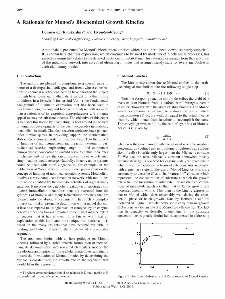
where µ is the maximum growth rate attained when the substrateconcentration (defined per unit volume of culture, i.e., suspen-sion of cells) is sufficiently larger than the Michaelis constantK. We use the term Michaelis constant somewhat looselybecause its usage is reserved for enzyme-catalyzed reactions inwhich it can be expressed in terms of rate constants associatedwith elementary steps. In the use of Monod kinetics, it is morecustomary to describe K as a “half saturation” constant whichrepresents the concentration of substrate at which the growthrate is half the maximum possible rate. For substrate concentra-tions of magnitude much less than that of K, the growth rateincreases linearly with s. This then is the kinetic expressiondue to Monod which does reasonably well during the expo-nential phase of batch growth. Data by Herbert et al.2 areincluded in Figure 1 which shows some early data on growthof Aerobacter cloacae fitted to Monod growth kinetics. The factthat its capacity to describe phenomena at low substrateconcentrations is greatly diminished is suppressed in addressing

* To whom correspondence should be addressed: E-mail: [email protected]; [email protected]. Figure 1. Data from Herbert et al. (1956) in support of Monod kinetics.

Ind. Eng. Chem. Res. 2008, 47, 9090–90989090

10.1021/ie800905d CCC: $40.75 2008 American Chemical SocietyPublished on Web 11/08/2008

batch growth but readily exposed by its failure to makepredictions in continuous cultures at lower dilution rates. Themaximum dilution rate (above which washout of cells from thereactor occurs) is, however, predicted by the Monod model withsome reasonableness. There have been many discussions in theliterature seeking to improve the prediction of growth dynamicsby the Monod model with other growth laws but are not ofsignificance to this paper as we are more concerned withderiving Monod′s model as an approximation from more detailedview of metabolism as a whole.

3. Stoichiometric Formulation of Metabolism

We will limit ourselves to central carbon metabolism in whichthe carbon source is admitted into the metabolic network inmany different ways. Metabolism involves uptake of thesubstrate followed by numerous intracellular reactions. Weassume that there are a total of R reactions numbered from 1 toR and represented by

-σiS+∑j)1

n

VijMj+∑r)1

p

πirPr ) 0, i) 1, 2, ..., R (3)

In eq 3, Mj, j ) 1, 2, ..., n, represent the intracellular metabolites,and Pr, r ) 1, 2, ..., p, represent the fermentation productsreleased into the abiotic environment. The stoichiometricconstant σi for the substrate S is generally non-negative as weenvisage only uptake of the substrate and forbid for our purposesany circumstance of it also arising as a fermentation product.For intracellular reactions, however, σi ) 0. The stoichiometriccoefficients νij can assume both positive (when Mj is a product)and negative (when it is a reactant). The stoichiometriccoefficients πir of the fermentation products Pr will be regardedas positive disregarding the possibility that some could reenterthe cell as a substrate. That some or all of the intracellularreactions can be reversible is already accommodated by theallowable signs of the stoichiometric coefficients. We denote

by U the set of indices for reactions in which substrate uptakeoccurs.

Denoting the consumption of substrate in the ith reaction byrs,i and the total consumption by rs, we see that

rs )∑i∈ U

rs,i (4)

Letting mj, j ) 1, 2, ..., n, denote the intracellular metabolitelevels (mass fractions relative to the total biomass), it is usualto make the pseudosteady state approximation for each of themetabolites which gives

∑i)1

R

Vijri - rGmj ) 0, j) 1, 2,..., n (5)

The second term on the left-hand side of eq 5 is the dilutionterm due to biomass growth whose origin was pointed out byFredrickson.3 The term is generally negligible for individualmetabolites so that a satisfactory representation of eq 5 is

∑i)1

R

Vijri ) 0, j) 1, 2,..., n (6)

Thus the reaction rates, ri, i ) 1, 2, ..., R or more commonlyreferred to in the biological literature as “fluxes” form a rowvector rT ≡ (r1, r2, ..., rn) which must be in the null space ofthe matrix N ≡ {νij; i ) 1, 2, ..., R; j ) 1, 2, ..., n} since eq 6implies that rTN ) 0. Alternatively, the column vector r mayalso be viewed as in the null space of NT, as NTr ) 0. At thispoint the flux balance approach of Palsson and co-workers (seeEdwards et al.4 for example) is to determine vectors in the nullspace of NT that would satisfy the criterion of maximizing anobjective function such as the biomass yield and determine theflux vector up to a multiplicative constant. A measurement ofthe total substrate uptake rate rs would then provide the uniqueflux vector of interest. Since this would of course yield thebiomass synthesis rate, the problem of providing a rationale for

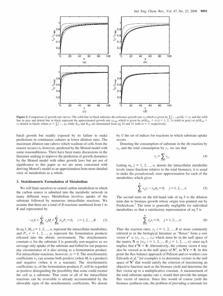
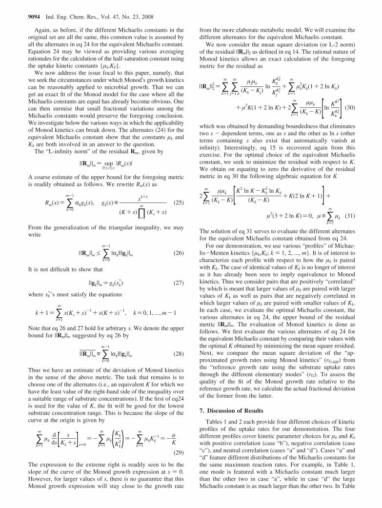
Figure 2. Comparison of growth rate curves: The solid line in black indicates the reference growth rate rG which is given by ∑k ) 13 µk/(Kk + s), and the solid

line in gray and dotted line in black represent the approximated growth rate rG,app which is given by µ/(Kalt,j + s) (j ) 1, 2, 3) (solid in gray) or µ/(Kopt +s) (dotted in black) where µ ) ∑k ) 1

3 µk while Kalt and Kopt are determined from eq 24 and 31 with m ) 3, respectively.

Ind. Eng. Chem. Res., Vol. 47, No. 23, 2008 9091

Monod kinetics boils down to showing that the sum of manyenzyme-catalyzed substrate uptake rates can be represented bya single enzyme substrate kinetic expression. Although this isbasically the approach of rationalization of this paper, wepostpone this specific step to a subsequent stage in the interestof expounding a more detailed view of metabolism broughtabout by the decomposition of the metabolic network intoelementary modes.

4. Decomposition of Metabolic Network into ElementaryModes

A particularly interesting way to view a metabolic networkappears to be in terms of elementary modes.5,6 An elementarymode is a part of the network which involves the uptake ofsubstrate, leading it through a sequence of reactions ultimatelyproducing one or more metabolic products and precursors forbiomass synthesis. Thus the flux vector has only positivecomponents in an elementary mode. The set of elementarymodes forms a convex set and will form a convex basis of thenull space of the matrix NT if all exchange fluxes are irreversibleor the convex cone (NTr ) 0; ri g 0, i ) 1, 2, ..., n). Theproblem of identifying the elementary modes for an arbitrarymetabolic network has been thoroughly investigated by Schusteret al.7 Elementary modes can be very substantial in number.Reversible reactions are accommodated in separate elementarymodes so that the “backward” reaction rate is also entered as apositive component in a mode different from that which hasthe forward reaction rate.

We assume that there are m elementary modes in all. Eachmode represents a vector of non-negative fluxes (reaction rates)to be determined uniquely only when the substrate uptake ratethrough that mode is known. Given that the reactions have alsobeen identified for each mode, we may represent each modealso by the reactions involved as follows.

-σiS+∑j)1

n

VijMj +∑r)1

p

πirPr ) 0, i ∈ Uk, k) 1, 2, ..., m

(7)

where {Uk}k ) 1m are subsets of {1, 2, ..., R} with Uk representing

the selection of reactions from the network for the kth mode.Since the different modes exhaust all reactions in metabolism,

we have ∪k)1

mUk ) U. The steady state balance of reactions in the

kth mode is given by replacing eq6 by

∑i∈ Uk

Vijri ) 0, j) 1, 2, ..., n, k) 1, 2, ..., m (8)

Clearly in eq8 we may set ri ) 0 for any reaction not includedin the mode. What distinguishes eq 8 from eq 6 is the fact thateq 8 has only one linearly independent solution for each k, whichwe denote by rk ≡ [r1

k, r2k, ..., rR

k]; k ) 1, 2, ..., m. It will beunderstood that the first component r1

k in the vector representsthe substrate uptake rate through that mode. Since it is only thetotal uptake rate of substrate that is known, the uptake ratethrough a given mode is known only up to a multiplicativeconstant. Thus, the total uptake rate of substrate is then givenby

rs )∑k)1

m

wkr1k (9)

where wk values are positiVe weights. The total uptake ofsubstrate is thus viewed to be distributed among variouselementary modes. Furthermore, we may define the uptake (row)

vector by r1T ≡ [r1

1, r12, ..., r1

m], so that the entire reaction ratevector r may be represented by

r )Zr1 (10)

The matrix Z in the equation above arises out of expanding thereaction rate vector r in terms of the elementary mode fluxvectors and representing each of the latter in terms of the uptakeflux through the mode. Thus we have the entire reaction ratevector depend only on the uptake flux vector r1 through theassumption of steady state for the intracellular components.

The growth rate of biomass is related to the intracellular fluxesand has been represented in the biological literature (seeStephanopoulos et al.8) by rG ) hTr, where the row vector hT

is available. Thus the growth rate may be expressed in terms ofthe uptake vector as

rG ) hTZr1 (11)

From eq 9, we can describe the total uptake rate of substrateby rs ) wTr1, where the row vector wT ≡ [w1, w2, ..., wm]. Theyield coefficient Y defined earlier in representing growth fromunit mass of the carbon substrate is given by

rs

rG) Y)

wTr1

hTZr1

(12)

Expression 12 shows substrate dependence of the yield coef-ficient which is acknowledged although not an original aspectof Monod′s model.

5. View of Metabolism through Elementary Modes

The viewpoint of metabolism that emerges from the foregoingperspective consists in envisaging substrate uptake through eachof the elementary modes. Denoting by wk the fraction (of thetotal substrate uptake rate) through the kth elementary mode, itis now possible to calculate all intracellular and extracellularfluxes connected with fermentation products. The weightfractions for the different modes are governed by the phenom-enon of metabolic regulation. Their calculation would in factrequire a detailed treatment of all the reactions in the cell withdue account of regulatory processes, clearly a problem ofinspiring magnitude. However, if we take refuge in the pseu-dosteady state hypothesis, the uptake rate through each modecould be stoichiometrically related to the intracellular fluxesthrough that mode. The uptake rates through the different modeshave then been modeled by Michaelis-Menten kinetics withconstants(µ′k,Kk),k ) 1,2, ..., m (see e.g., Provost et al.9). Theimplication of this approach is that uptake can be modeled bysingle substrate enzyme kinetics that could be varied for eachof the modes to account for the regulatory effects in each mode.The total uptake rate of the substrate denoted rs can then bewritten as

rs )∑k)1

m µ′ks

Kk + s

The growth rate rG may then be written as

rG )∑k)1

m µks

Kk + sµk ≡∑

i

hizikµ′k (13)

where zik is the (i,k)th coefficient of the matrix Z.

6. Approximation of Growth Rate by Monod Kinetics

We wish to approximate ∑k ) 1m µks/(Kk + s) by the expression

µs/(K + s) and seek the best choice of µ and K given the values

9092 Ind. Eng. Chem. Res., Vol. 47, No. 23, 2008

of {(µ1,K1), (µ2,K2), ..., (µm,Km)} for each of the Michaelis-Menten kinetic expressions for the uptake reactions for thedifferent modes. Alternatively, we seek to minimize the residual

Rm(s) ≡ rG -µs

(K+ s))∑

k)1

m µks

(Kk + s)- µs

(K+ s)

As a measure of the quality of the approximation, we consideron the space of functions defined on both the metrics | |∞ and| |2 defined by

(1) |f|∞ ≡ sup0exes

|f(x)|

(2) |f|22 ≡∫0

sf(x)2 dx (14)

The residual is represented by the vector Rm ≡ {Rm(x): 0 e xe s}. The upper limit s can of course be increased indefinitely.The two norms in eq 14 for the residual represent differentmeasures. The first is less forgiving of large deviations even ina small localized zone than the second. The second measure isperhaps sufficient but the first has the advantage of producingvarious candidates for the effective Michaelis constant forMonod kinetics. We shall consider both the measures in eq14.

Let us address at first the first metric in (14). Since it isconcerned with deviation at each point s, for suitably largevalues of s (considerably larger than the largest Michaelisconstant in the set {Kk:k ) 1,2, ..., m}), the growth rate rG isgiven by the sum of the maximum rates from each of the modesso that

µ)∑k)1

m

µk (15)

The Michaelis constant for the Monod model is then to bedetermined so that the residual is minimal in some sense.Toward this end, we consider below the case of m ) 3for simplicity before stating the general case. It is conve-nient to begin by exploring the behavior of f3(s) ≡(K1+s)(K2+s)(K3+s)(K+s)R3(s)/s which is given by

µ1(K+ s)(K2 + s)(K3 + s)+ µ2(K+ s)(K3 + s)(K1 + s)+µ1(K+ s)(K1 + s)(K2 + s)- µ(K1 + s)(K2 + s)(K3 + s))

[K(µ1K2K3 + µ2K3K1 + µ3K1K2)- µK1K2K3]+s[µ1(K2K3 +KK2 +KK3)+ µ2(K3K1 +KK3 +KK1)+µ3(K1K2 +KK1 +KK2)-µ(K1K2 +K2K3 +K3K1)]+

s2[µ1(K+K2 +K3)+ µ2(K+K3 +K1)+ µ3(K+K1 +K2)-µ(K1 +K2 +K3)] (16)

From eq 15, setting m ) 3, we have µ ) µ1 + µ2 + µ3. Insertingthis into eq 16 and equating each of the square brackets equalto zero, we have three different alternates for the value of Kfrom comparing coefficients of s0, s1, and s2.

K)µ1 + µ2 + µ3

µ1K1-1 + µ2K2

-1 + µ3K3-1

(17)

K)µ1K1(K2 +K3)+ µ2K2(K3 +K1)+ µ3K3(K1 +K2)

µ1(K2 +K3)+ µ2(K3 +K1)+ µ3(K1 +K2)(18)

K)µ1K1 + µ2K2 + µ3K3

µ1 + µ2 + µ3(19)

Of course eq17, 18, and 19 cannot be simultaneously true exceptfor when K1 ) K2 ) K3. It should be intuitively clear at thisstage that if K1, K2, K3 are not very disparate, one of theforegoing candidates could serve to be a reasonable Michaelis

constant for the Monod model. For m ) 4, by comparingcoefficients of s0, s1, s2, and s3, we respectively have

K)µ1 + µ2 + µ3 + µ4

µ1K1-1 + µ2K2

-1 + µ3K3-1 + µ4K4

-1(20)

K) [µ1K1(K2K3 +K2K4 +K3K4)+ µ2K2(K1K3 +K1K4 +K3K4)+

µ3K3(K1K2 +K1K4 +K2K4)+ µ4K4(K1K2 +K1K3 +K2K3)] ⁄

[µ1(K2K3 +K2K4 +K3K4)+ µ2(K1K3 +K1K4 +K3K4) +µ3(K1K2 +K1K4 +K2K4)+ µ4(K1K2 +K1K3 +K2K3)] (21)

K)∑k)1

4

µkKk ∑l)1,k

4

Kl

∑k)1

4

µk ∑l)1,k

4

Kl

(22)

K)∑k)1

4

µkKk

∑k)1

4

µk

(23)

The notation l ) 1, k is designed to exclude the running indexl from taking on the value of k. As in the case of m ) 3, wefind that if all the Michaelis constants are equal, then theformulas 20, 21, 22 and 23 all consistently yield the sameequivalent Michaelis constant. We now return to the generalcase of m modes. Toward this end, it is of interest to considerall combinations of r elements of the set Sm ≡ {1, 2, ..., m} anddenote this set by Cr(Sm). Identify the combinatory elements ofthis set with a discrete index, say i to associate uniquely with

a combination (i1, i2, ..., ir). Clearly there are (mr ) elements in

the set Cr(Sm). This notation can be conveniently used to expresscertain functions of the combinations. For example, the term∑ i∈ Cr(Sm) ∏k)1

r Kikrepresents the sum of all possible products of

r distinct Michaelis constants obtained from the original set ofm constants. It is necessary to introduce one further notation.A specific element, say k may be omitted from the set Sm, whichmay be denoted by Sm,k before seeking r combinations of them.With this notation, it is now possible to return to the generalcase of m elementary modes. We note that fm(s) containscoefficients, say R0, R1, ..., Rm-1 of s0, s1, s2, ..., sm-1,respectively, each of which can be equated to zero to producem alternates for the equivalent Michaelis constant. These canbe seen to be respectively

K)∑k)1

m

µk

∑k)1

m

µkKk-1

(j) 0),

K)∑k)1

m

µkKk ∑i∈ Cm-j-1(Sm,k)

∏r)1

m-j-1

Kir

∑k)1

m

µk ∑i∈ Cm-j-1(Sm,k)

∏r)1

m-j-1

Kir

(j) 1, 2, ..., m- 2),

K)∑k)1

m

µkKk

∑k)1

m

µk

(j)m- 1) (24)


Again, as before, if the different Michaelis constants in theoriginal set are all the same, this common value is assumed byall the alternates in eq 24 for the equivalent Michaelis constant.Equation 24 may be viewed as providing various averagingrationales for the calculation of the half-saturation constant usingthe uptake kinetic constants {µk,Kk}.

We now address the issue focal to this paper, namely, thatwe seek the circumstances under which Monod′s growth kineticscan be reasonably applied to microbial growth. That we canget an exact fit of the Monod model for the case where all theMichaelis constants are equal has already become obvious. Onecan then surmise that small fractional variations among theMichaelis constants would preserve the foregoing conclusion.We investigate below the various ways in which the applicabilityof Monod kinetics can break down. The alternates (24) for theequivalent Michaelis constant show that the constants µk andKk are both involved in an answer to the question.

The “L-infinity norm” of the residual Rm, given by

|Rm|∞ ) sup0exes

|Rm(x)|

A coarse estimate of the upper bound for the foregoing metricis readily obtained as follows. We rewrite Rm(x) as

Rm(x)) ∑k)0

m-1

Rkgk(x), gk(x) ≡ xk+1

(K+ x)∏r)1

m

(Kr + x)

(25)

From the generalization of the triangular inequality, we maywrite

|Rm|∞e∑k)0

m-1

|Rk||gk|∞ (26)

It is not difficult to show that

|gk|∞ ) gk(xk*) (27)

where xk*’s must satisfy the equations

k+ 1)∑r)1

m

x(Kr + x)-1 + x(K+ x)-1, k) 0, 1, ..., m- 1

Note that eq 26 and 27 hold for arbitrary s. We denote the upperbound for |Rm|∞ suggested by eq 26 by

|Rm|∞ ≡ ∑k)0

m-1

|Rk||gk|∞ (28)

Thus we have an estimate of the deviation of Monod kineticsin the sense of the above metric. The task that remains is tochoose one of the alternates (i.e., an equivalent K for which wehave the least value of the right-hand side of the inequality overa suitable range of substrate concentrations). If the first of eq24is used for the value of K, the fit will be good for the lowestsubstrate concentration range. This is because the slope of thecurve at the origin is given by

∑k)1

m

µkdds[ s

Kk + s]s)0)-∑

k)1

m

µk(Kk

Kk2))-∑

k)1

m

µkKk-1 )-µ

K

(29)

The expression to the extreme right is readily seen to be theslope of the curve of the Monod growth expression at s ) 0.However, for larger values of s, there is no guarantee that thisMonod growth expression will stay close to the growth rate

from the more elaborate metabolic model. We will examine thedifferent alternates for the equivalent Michaelis constant.

We now consider the mean square deviation (or L-2 norm)of the residual |Rm|2 as defined in eq 14. The rational nature ofMonod kinetics allows an exact calculation of the foregoingmetric for the residual as

|Rm|22 )∑

k)1

m

∑j)1,k

m µjµk

(Kk -Kj)ln

KkKk

2

KjKj

2+∑

k)1

m

µk2Kk(1+ 2 ln Kk)

+ µ2K(1+ 2 ln K)+ 2∑k)1

m µµk

(Kk -K)[lnKK2

KkKk

2] (30)

which was obtained by demanding boundedness that eliminatestwo s - dependent terms, one as s and the other as ln s (otherterms containing s also exist that automatically vanish atinfinity). Interestingly, eq 15 is recovered again from thisexercise. For the optimal choice of the equivalent Michaelisconstant, we seek to minimize the residual with respect to K.We obtain on equating to zero the derivative of the residualmetric in eq 30 the following algebraic equation for K

2∑k)1

m µµk

(Kk -K)[K2 ln K-Kk2 ln Kk

(Kk -K)+K(2 ln K+ 1)] +

µ2(3+ 2 ln K)) 0, µ ≡∑k)1

m

µk (31)

The solution of eq 31 serves to evaluate the different alternatesfor the equivalent Michaelis constant obtained from eq 24.

For our demonstration, we use various “profiles” of Michae-lis-Menten kinetics {µk,Kk; k ) 1, 2, ..., m}. It is of interest tocharacterize each profile with respect to how the µk is pairedwith Kk. The case of identical values of Kk is no longer of interestas it has already been seen to imply equivalence to Monodkinetics. Thus we consider pairs that are positively “correlated”by which is meant that larger values of µk are paired with largervalues of Kk as well as pairs that are negatively correlated inwhich larger values of µk are paired with smaller values of Kk.In each case, we evaluate the optimal Michaelis constant, thevarious alternates in eq 24, the upper bound of the residualmetric |Rm|∞. The evaluation of Monod kinetics is done asfollows. We first evaluate the various alternates of eq 24 forthe equivalent Michaelis constant by comparing their values withthe optimal K obtained by minimizing the mean square residual.Next, we compare the mean square deviation of the “ap-proximated growth rates using Monod kinetics” (rG,app) fromthe “reference growth rate using the substrate uptake ratesthrough the different elementary modes” (rG). To assess thequality of the fit of the Monod growth rate relative to thereference growth rate, we calculate the actual fractional deviationof the former from the latter.

7. Discussion of Results

Tables 1 and 2 each provide four different choices of kineticprofiles of the uptake rates for our demonstration. The fourdifferent profiles cover kinetic parameter choices for µk and Kk

with positive correlation (case “b”), negative correlation (case“c”), and neutral correlation (cases “a” and “d”). Cases “a” and“d” feature different distributions of the Michaelis constants forthe same maximum reaction rates. For example, in Table 1,one mode is featured with a Michaelis constant much largerthan the other two in case “a”, while in case “d” the largeMichaelis constant is as much larger than the other two. In Table


2, case “d” features one mode with an even larger Michaelisconstant. Each row of Tables 1 and 2 is divided into threesubrows in the third and fourth columns. In the third column,among three subrows, the top shows Kalt,j (j ) 1, 2, ..., m) (the

alternates to equivalent Michaelis constant K) and the middleand bottom show |Rm|∞ (the upper bound of L-infinity normof the residual) and |Rm|2 (the L-2 norm of the residual),respectively, when K ) Kalt, while, in the end column, the top

Table 1. Parameter Values Used for Plotting the Curves Shown in Figure 1 and the Residual Normsa

figures {µ1, µ2, µ3} {K1, K2, K3}Kalt () alternates of K)|R3|∞(K ) Kalt)|R3|2(K ) Kalt)

Kopt () optimal K)|R3|∞(K ) Kopt)|R3|2(K ) Kopt)

Figure 2a {1/3, 1/3, 1/3} {0.1, 2, 10} {0.283, 1.752, 4.033} 2.788{0.423, 0.243, 0.315} 0.291{1.210, 0.497, 0.495} 0.333

Figure 2b {0.1, 0.2, 0.7} {0.1, 2, 10} {0.855, 4.021, 7.410} 6.611{0.488, 0.154, 0.132} 0.139{1.807, 0.664, 0.258} 0.194

Figure 2c {0.7, 0.2, 0.1} {0.1, 2, 10} {0.141, 0.657, 1.470} 0.618{0.199, 0.288, 0.442} 0.289{0.486, 0.266, 0.515} 0.265

Figure 2d {1/3, 1/3, 1/3} {1, 2.5, 5} {1.875, 2.353, 2.833} 2.583{0.070, 0.043, 0.065} 0.055{0.279, 0.109, 0.111} 0.070

a Three elementary modes are considered. |R3|∞ and |R3|2 indicate the upper bound of the L-infinity norm of residual, and the L-2 norm,respectively, for three elementary modes.

Table 2. Parameter Values Used for Plotting the Curves Shown in Figure 2 and the Residual Normsa

figures {µ1, µ2, ..., µ10} {K1, K2, ..., K10}Kalt () alternates of K)|R10|∞ (K ) Kalt)|R10|2 (K ) Kalt)

Kopt () optimalK)|R10|∞ (K ) Kopt)|R10|2 (K ) Kopt)

Figure 3a {1/10, 1/10, ..., 1/10} {0.1, 0.2, 0.4, 0.8, 1.6, 3.2,6.4, 12.8, 25.6, 51.2}

{0.709, 1.311, 1.5808, 1.742,1.861, 1.962, 2.062, 2.178,2.338, 2.610}

5.6406

{ 0.684, 0.571, 0.476, 0.408,0.372, 0.372, 0.408, 0.476,0.571, 0.684}

0.486

{ 1.770, 1.676, 1.553, 1.398,1.208, 0.988, 0.768, 0.641,0.753, 1.081}

0.640

Figure 3b {0.0010, 0.0020, 0.0039,0.0078, 0.0156, 0.0313,0.0626, 0.1251, 0.2502,0.5005}

{0.1, 0.2, 0.4, 0.8, 1.6, 3.2,6.4, 12.8, 25.6, 51.2}

{10.230, 11.311, 12.618,14.213, 16.168, 18.571,21.511, 25.069, 29.293,34.167}

31.110

{0.386, 0.342, 0.295, 0.247,0.198, 0.153, 0.116, 0.095,0.097, 0.129}

0.110

{2.686, 2.506, 2.299, 2.059,1.782, 1.464, 1.104, 0.711,0.349, 0.423}

0.294

Figure 3c {0.5005, 0.2502, 0.1251,0.0626, 0.0313, 0.0156,0.0078, 0.0039, 0.0020,0.0010}

{0.1, 0.2, 0.4, 0.8, 1.6, 3.2,6.4, 12.8, 25.6, 51.2}

{0.150, 0.175, 0.204, 0.238,0.276, 0.317, 0.360, 0.406,0.453, 0.501}

0.252

{0.129, 0.097, 0.095, 0.116,0.153, 0.198, 0.247, 0.295,0.342, 0.386}

0.130

{0.147, 0.119, 0.094, 0.077,0.080, 0.101, 0.132, 0.167,0.203, 0.239}

0.076

Figure 3d {1/10, 1/10, ..., 1/10} {0.1, 2.01, 2.02, 2.03, 2.04,2.05, 2.06, 2.07, 2.08,51.2}

{0.713, 1.335, 1.618, 1.797,1.939, 2.078, 2.247, 2.509,3.097, 6.730}

3.206

{0.527, 0.254, 0.186, 0.160,0.151, 0.151, 0.161, 0.188,0.261, 0.585}

0.275

{1.087, 0.789, 0.684, 0.625,0.583, 0.546, 0.506, 0.455,0.400, 0.947}

0.399

a Ten elementary modes are considered. |R10|∞ and |R10|2 indicate the upper bound of the L-infinity norm of residual, and the L-2 norm,respectively, for 10 elementary modes.


shows Kopt (the optimum choice of K) and the middle andbottom show |Rm|∞ and |Rm|2, respectively, when K ) Kopt.

Figures 2 and 3 show the results of our evaluation of Kalt,j (j) 1, 2, ..., m) and Kopt for the half-saturation constant in Monodkinetics for various types of kinetic profiles of the uptake rates.The number of elementary modes “m” was assumed to be “3”in Figure 2 and “10” in Figure 3, and the reference growthcurves (solid line in black, rG) were obtained from eq 13 withthe sets of µk and Kk as given in Tables 1 and 2, respectively.The various Monod kinetics approximating rG are denoted byrG,app where the equivalent Michaelis constant is given by Kalt,j

(j ) 1, 2, ..., m) (solid line in gray) or Kopt (dotted line).Figure 2a shows results for a “neutral” kinetic profile

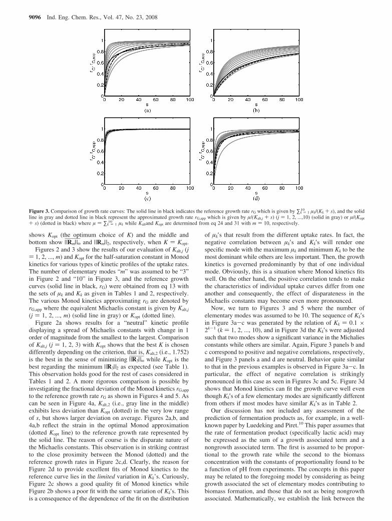
displaying a spread of Michaelis constants with change in 1order of magnitude from the smallest to the largest. Comparisonof Kalt,j (j ) 1, 2, 3) with Kopt shows that the best K is chosendifferently depending on the criterion, that is, Kalt,2 (i.e., 1.752)is the best in the sense of minimizing |R3|∞ while Kopt is thebest regarding the minimum |R3|2 as expected (see Table 1).This observation holds good for the rest of cases considered inTables 1 and 2. A more rigorous comparison is possible byinvestigating the fractional deviation of the Monod kinetics rG,app

to the reference growth rate rG as shown in Figures 4 and 5. Ascan be seen in Figure 4a, Kalt,2 (i.e., gray line in the middle)exhibits less deviation than Kopt (dotted) in the very low rangeof s, but shows larger deviation on average. Figures 2a,b, and4a,b reflect the strain in the optimal Monod approximation(dotted Kopt line) to the reference growth rate represented bythe solid line. The reason of course is the disparate nature ofthe Michaelis constants. This observation is in striking contrastto the close proximity between the Monod (dotted) and thereference growth rates in Figure 2c,d. Clearly, the reason forFigure 2d to provide excellent fits of Monod kinetics to thereference curve lies in the limited variation in Kk’s. Curiously,Figure 2c shows a good quality fit of Monod kinetics whileFigure 2b shows a poor fit with the same variation of Kk′s. Thisis a consequence of the dependence of the fit on the distribution

of µk′s that result from the different uptake rates. In fact, thenegative correlation between µk′s and Kk′s will render onespecific mode with the maximum µk and minimum Kk to be themost dominant while others are less important. Then, the growthkinetics is governed predominantly by that of one individualmode. Obviously, this is a situation where Monod kinetics fitswell. On the other hand, the positive correlation tends to makethe characteristics of individual uptake curves differ from oneanother and consequently, the effect of disparateness in theMichaelis constants may become even more pronounced.

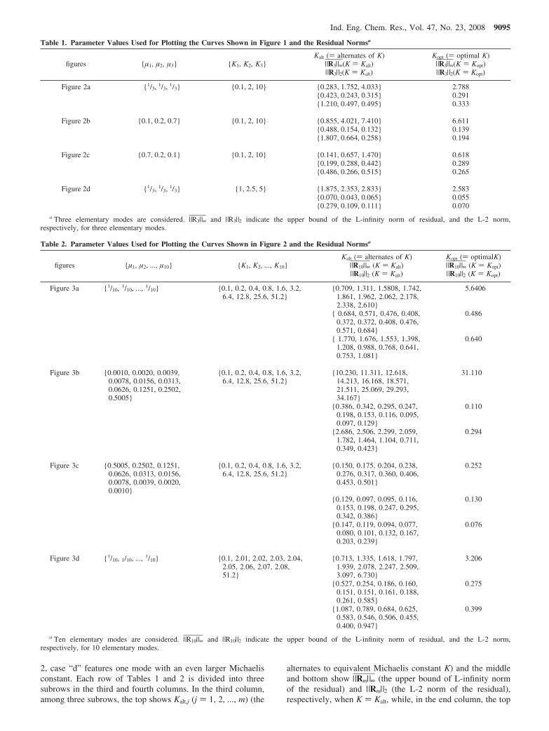
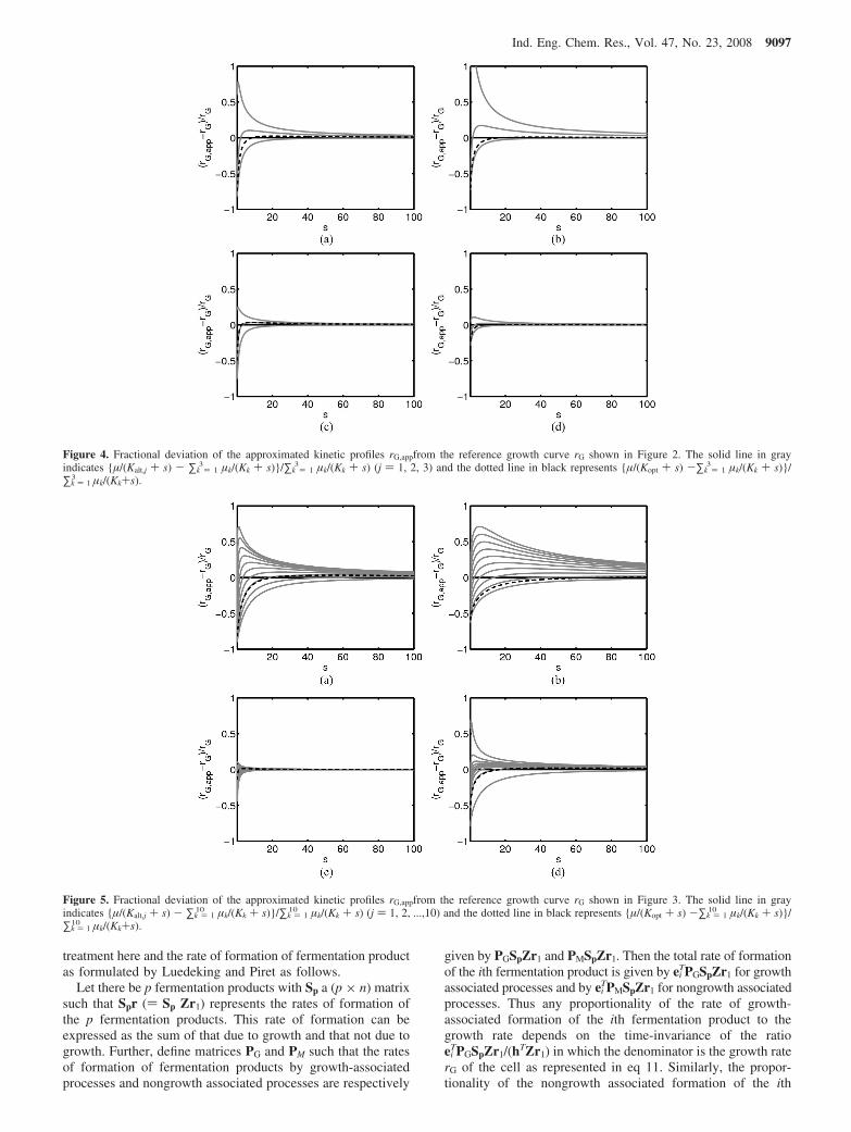
Now, we turn to Figures 3 and 5 where the number ofelementary modes was assumed to be 10. The sequence of Kk′sin Figure 3a-c was generated by the relation of Kk ) 0.1 ×2k-1 (k ) 1, 2, ..., 10), and in Figure 3d the Kk′s were adjustedsuch that two modes show a significant variance in the Michaliesconstants while others are similar. Again, Figure 3 panels b andc correspond to positive and negative correlations, respectively,and Figure 3 panels a and d are neutral. Behavior quite similarto that in the previous examples is observed in Figure 3a-c. Inparticular, the effect of negative correlation is strikinglypronounced in this case as seen in Figures 3c and 5c. Figure 3dshows that Monod kinetics can fit the growth curve well eventhough Kk′s of a few elementary modes are significantly differentfrom others if most modes have similar Kk′s as in Table 2.

Our discussion has not included any assessment of theprediction of fermentation products as, for example, in a well-known paper by Luedeking and Piret.10 This paper assumes thatthe rate of fermentation product (specifically lactic acid) maybe expressed as the sum of a growth associated term and anongrowth associated term. The first is assumed to be propor-tional to the growth rate while the second to the biomassconcentration with the constants of proportionality found to bea function of pH from experiments. The concepts in this papermay be related to the foregoing model by considering as beinggrowth associated the set of elementary modes contributing tobiomass formation, and those that do not as being nongrowthassociated. Mathematically, we establish the link between the

Figure 3. Comparison of growth rate curves: The solid line in black indicates the reference growth rate rG which is given by ∑k ) 110 µk/(Kk + s), and the solid

line in gray and dotted line in black represent the approximated growth rate rG,app which is given by µ/(Kalt,j + s) (j ) 1, 2, ...,10) (solid in gray) or µ/(Kopt

+ s) (dotted in black) where µ ) ∑k ) 110 µk while Kaltand Kopt are determined from eq 24 and 31 with m ) 10, respectively.


treatment here and the rate of formation of fermentation productas formulated by Luedeking and Piret as follows.

Let there be p fermentation products with Sp a (p × n) matrixsuch that Spr () Sp Zr1) represents the rates of formation ofthe p fermentation products. This rate of formation can beexpressed as the sum of that due to growth and that not due togrowth. Further, define matrices PG and PM such that the ratesof formation of fermentation products by growth-associatedprocesses and nongrowth associated processes are respectively

given by PGSpZr1 and PMSpZr1. Then the total rate of formationof the ith fermentation product is given by ei

TPGSpZr1 for growthassociated processes and by ei

TPMSpZr1 for nongrowth associatedprocesses. Thus any proportionality of the rate of growth-associated formation of the ith fermentation product to thegrowth rate depends on the time-invariance of the ratioei

TPGSpZr1/(hTZr1) in which the denominator is the growth raterG of the cell as represented in eq 11. Similarly, the propor-tionality of the nongrowth associated formation of the ith

Figure 4. Fractional deviation of the approximated kinetic profiles rG,appfrom the reference growth curve rG shown in Figure 2. The solid line in grayindicates {µ/(Kalt,j + s) - ∑k ) 1

3 µk/(Kk + s)}/∑k ) 13 µk/(Kk + s) (j ) 1, 2, 3) and the dotted line in black represents {µ/(Kopt + s) -∑k ) 1

3 µk/(Kk + s)}/∑k ) 1

3 µk/(Kk+s).

Figure 5. Fractional deviation of the approximated kinetic profiles rG,appfrom the reference growth curve rG shown in Figure 3. The solid line in grayindicates {µ/(Kalt,j + s) - ∑k ) 1

10 µk/(Kk + s)}/∑k ) 110 µk/(Kk + s) (j ) 1, 2, ...,10) and the dotted line in black represents {µ/(Kopt + s) -∑k ) 1

10 µk/(Kk + s)}/∑k ) 1

10 µk/(Kk+s).


fermentation product depends on the time invariance ofei

TPMSpZr1. The time-invariance of both quantities depends uponthe time-invariance of the uptake rate vector r1. For large enoughconcentration of the substrate, we expect r1 to be time-invariantthus vindicating the Luedeking and Piret approach. However,when the substrate concentration drops to small values, regula-tory effects associated with growth and maintenance will nolonger sustain the assumptions made by Luedeking and Piret.

8. Factors Against Monod Kinetics

While support for Monod growth kinetics could be obtainedfrom viewing metabolism as being the result of substrate uptakethrough several elementary modes, it was assumed that therelative distribution of substrate through different modes remainslargely invariant. This is in fact not true as one is well awarethat at very low substrate concentrations, the organisms regulatetheir metabolism to consume substrate more for maintenanceof viability than for growth. This means that the kinetic profilesare themselves subject to change under different conditions. Thissituation is manifestly apparent in continuous cultures butvirtually invisible in batch growth as change in biomass doesnot occur toward the end of batch growth. Thus the applicabilityof Monod kinetics to continuous cultures leads to a constantbiomass concentration at steady state regardless of the dilutionrate (flow rate/hold-up volume) as long at it is below themaximum dilution rate. Experimental data, on the other hand,show decrease in steady state concentration of biomass presum-ably due to maintenance effects.

Clearly, the complexities of regulatory processes cannot bedescribed by Monod′s growth kinetics. As long as the Michaelisconstants are not widely disparate, Monod’s growth kineticshas a domain of application, however. With respect to theapplicability of Monod kinetics the scenario of equal Michaelisconstants is not very different from that when the Michaelisconstants are not widely disparate. When regulatory processesare accounted for, however, even small differences in Michaelisconstants lead to rather complex behavior in continuous cultures.Kim11 has recently shown that both steady state multiplicityand oscillatory dynamics can result with the cybernetic modelsof Ramkrishna and co-workers.12-15

9. Conclusions

This paper has demonstrated that a rationale exists for theapplicability of Monod′s growth kinetics. It also shows how itsfailure must be expected as it cannot accept the burden ofdescribing regulatory processes. Monod kinetics becomes at-tractive when the Michaelis constants are not widely disparatebut even when they are the existence of negative correlationcan give rise to reasonable Monod approximations to the growthrate. The reason for the latter can be explained by the

predominance of one specific mode with the maximum µk andminimum Kk. Even in the case that a few Kk’s are significantlydifferent from the others, the quality of fit by Monod equationcan be good if most of Kk’s have similar values. On the otherhand, Monod kinetics may fail when Kk’s show significantvariance and µk’s vary independently of Kk or Kk’s have positivecorrelation with µk’s.

Literature Cited

(1) Wei, J.; Kuo, J. C. W. A lumping analysis in monomolecular reactionsystems: Analysis of the exactly lumpable system. Ind. Eng. Chem. Fundam.1969, 8, 114.

(2) Herbert, D.; Elsworth, R.; Telling, R. C. The continuous culture ofbacteriasA theoretical and experimental study. J. Gen. Microbiol. 1956,14, 601.

(3) Fredrickson, A. G. Formulation of structured growth models.Biotechnol. Bioeng. 1976, 18, 1481.

(4) Edwards, J. S.; Ibarra, R. U.; Palsson, B. O. In silico predictions ofEscherichia coli metabolic capabilities are consistent with experimental data.Nat. Biotechnol. 2001, 19, 125.

(5) Schuster, S.; Dandekar, T.; Fell, D. A. Detection of elementary fluxmodes in biochemical networks: a promising tool for pathway analysis andmetabolic engineering. Trends Biotechnol. 1999, 17, 53.

(6) Schuster, S.; Fell, D. A.; Dandekar, T. A general definition ofmetabolic pathways useful for systematic organization and analysis ofcomplex metabolic networks. Nat. Biotechnol. 2000, 18, 326.

(7) Schuster, S.; Hilgetag, C; Woods, J. H.; Fell, D. A. Reaction routesin biochemical reaction systems: Algebraic properties, validated calculationprocedure and example from nucleotide metabolism. J. Math. Biol. 2002,45, 153.

(8) Stephanopoulos, G.; Aristidou, A. A.; Nielsen, J. MetabolicEngineeringsprinciples and Methodologies; Academic Press: San Diego,CA, 1998.

(9) Provost, A.; Bastin, G.; Agathos, S. N.; Schneider, Y.-J. Metabolicdesign of macroscopic bioreaction models: Application to Chinese hamsterovary cells. Bioprocess Biosyst. Eng. 2006, 29, 349.

(10) Luedeking, R.; Piret, E. L. A kinetic study of lactic acid fermenta-tion-batch process at controlled pH. J. Biochem. Microbiol. Technol. Eng.1959, 1, 393.

(11) Kim, J. I. , A hybrid cybernetic modeling of the growth forEscherichia coli in glucose-pyruvate mixtures. Ph.D. Thesis. PurdueUniversity, West Lafayette, IN, 2008.

(12) Kompala, D. S.; Ramkrishna, D.; Jansen, N. B.; Tsao, G. T.Investigation of bacterial-growth on mixed substrates - Experimentalevaluation of cybernetic models. Biotechnol. Bioeng. 1986, 28, 1044.

(13) Young, J. D.; Ramkrishna, D. On the matching and proportionallaws of cybernetic models. Biotechnol. Progress 2007, 23, 83.

(14) Young, J. D.; Henne, K. L.; Morgan, J. A.; Konopka, A. E.;Ramkrishna, D. Integrating cybernetic modeling with pathway analysis. Adynamic systems level description of metabolic control. Biotechnol. Bioeng.2008, 100, 542.

(15) Kim, J. I.; Varner, J. D.; Ramkrishna, D. A. hybrid model ofanaerobic E. coli GJT001: Combination of elementary flux modes andcybernetic variables. Biotechnol. Progress 2008, in press.

ReceiVed for reView June 9, 2008ReVised manuscript receiVed September 17, 2008

Accepted September 18, 2008

IE800905D


a rationale for monod′s biochemical growth kinetics

Documents