A Rational Inattention Theory of Echo Chamber

Lin Hu∗ Anqi Li† Xu Tan‡

This Draft: October 2021

Abstract

Finite players gather information about an uncertain state before making

decisions. Each player allocates his limited attention capacity between biased

sources and the other players, and the resulting stochastic attention network

facilitates the transmission of information from primary sources to him either

directly or indirectly through the other players. The scarcity of attention leads

the player to focus on his own-biased source, resulting in occasional cross-

cutting exposures but most of the time a reinforcement of his predisposition.

It also limits his attention to like-minded friends who, by attending to the

same primary source as his, serve as secondary sources in case the information

transmission from the primary source to him is disrupted. A mandate on

impartial exposures to all biased sources disrupts echo chambers but entails

ambiguous welfare consequences. Inside an echo chamber, even a small amount

of heterogeneity between players can generate fat-tailed distributions of public

opinion, and factors affecting the visibility of sources and players could have

unintended consequences for public opinion and consumer welfare.

∗Research School of Finance, Actuarial Studies and Statistics, Australian National University,lin.hu@anu.edu.au.

†Olin Business School, Washington University in St. Louis, angellianqi@gmail.com.‡Department of Economics, University of Washington, tauxu@uw.edu.

1

arX

iv:2

104.

1065

7v3

[ec

on.T

H]

4 O

ct 2

021

1 Introduction

The Cambridge English Dictionary defines echo chamber as “an environment in which

a person encounters only beliefs or opinions that coincide with their own, so that their

existing views are reinforced and alternative ideas are not considered.” Examples that

fit this definition have recently flourished on the Internet and social media (Adamic

and Glance (2005); Bakshy, Messing, and Lada (2015); Mosleh et al. (2021)), and

they could prove dire for political polarization, public health, and efforts to contain

misinformation and fake news (Del Vicario et al. (2016); Barbera (2020); Cossard et

al. (2020)). Existing theories of echo chamber focus on its behavioral roots (Levy and

Razin (2019)). This paper develops a rational theory of echo chamber and examines

its normative implications.

Our premise is Rational Inattention (RI), i.e., the rational and flexible allocation

of one’s limited attention span across the various news sources. Such a premise has

become increasingly relevant in today’s digital age, as more people get news from the

Internet and social media where the amount of available information (2.5 quintillion

bytes) is vastly greater than what any individual can process in a lifetime (Matsa and

Lu (2016)). Constrained by attentional bottlenecks, news consumers must be selective

about which websites to read and which people to follow on Facebook and Twitter.

Enabled by technology advancements, they can now personalize how much time to

spend on the various news sources based on their preferences, needs, demographic

and psychographic attributes, digital footprints, etc (Pariser (2011)).

In this paper, we take a simplistic view on news sources, modeling them as poten-

tially biased technologies rather than self-interest entities with persuasion or profit-

maximizing motives (see, however, an earlier draft of this paper for an extension).

Instead, we focus on how RI gives rise to echo chambers and affects the opinion distri-

2

bution inside an echo chamber. We also examine regulations of information platforms

in terms of their efficacy in disrupting echo chambers and in shaping public opinion

and consumer welfare.

Our analysis is conducted in a simple environment of decision-making under un-

certainties. To fix ideas, suppose there are two possible states of the world L and

R that occur with equal probability, depending on whether the Democratic or the

Republican candidate has a better quality. There are finitely many players, each of

whom can express support to one candidate by taking action L or R, and his utility

is the highest when his action matches the true state of the world. If the two objects

mismatch, then the player’s disutility depends on whether he is taking his default

action, i.e., supporting the candidate he horizontally prefers. Taking the default ac-

tion is optimal given the prior belief about the state distribution, and two players are

like-minded friends if they share the same default action.

There are two primary sources, e.g., newspapers, that specialize in the reporting

of different state realizations. In each state L or R, the source that specializes in its

reporting generates news about it, whereas the other source is deactivated. To make

informed decisions, players pay attention to primary sources and to other players by

spending valuable time with them. Attention is limited, and yet its allocation is fully

flexible: a feasible attention strategy for a player specifies the amount of attention he

pays to each source and to any other player, subject to the constraint that the total

amount of attention he pays mustn’t exceed his bandwidth.

After players decide on their attention strategies, the state is realized, and news is

circulated in the society for two rounds according to independent Poisson processes.

In the first round, the activated primary source disseminates news about the realized

state to players, and the probability that such news reaches a player increases with the

amount of attention the latter pays to the primary source. In the second round, each

3

player who learned about the state previously passes along the news as a secondary

source, and the probability that such news reaches another player increases with the

sender’s visibility parameter (e.g. domain-specific knowledge, socioeconomic status,

personality strength, desire to influence others, tech-savviness (Winter and Neubaum

(2016)) and the amount of attention the receiver pays to the sender. After that,

players update beliefs and take actions. We analyze pure strategy perfect Bayesian

equilibria of this game.

We interpret specialized reporting as a kind of source bias. Specifically, we define

player’s own-biased source as the source that generates disapproving news of his

default action, so that hearing no news from it reinforces the player’s belief that the

state favors his default action.1 We note that all like-minded friends share the same

own-biased source, and say that echo chambers arise in equilibrium if all players

limit attention to their own-biased sources and like-minded friends. In an echo-

chamber equilibrium, each player remains uninformed of the state with more than

fifty percent probability and reinforces his belief that the state favors his default

action in that event. That is, he is occasionally exposed to cross-cutting content

and updates his belief accordingly, but most of the time he gets his predisposition

reinforced. The coexistence of belief polarization and occasional belief reversal is a

hallmark of Bayesian rationality, and its presence after (social) media consumption

has recently been documented by the empirical literature.2

1Our notion of source bias isn’t new to the literature (see Section 1.1 for further discussions).According to it, a left-wing voter’s own-biased source is NY Times, because hearing no endorsementby NY Times for the Republican candidate reinforces the belief that the state favors the Democraticcandidate. According to Chiang and Knight (2011), newspaper endorsements of presidential can-didates are most effective in shaping voters’ beliefs and decisions if they go against the bias of thenewspaper.

2Flaxman, Goel, and Rao (2016) compare subjects’ ideological positions before and after Internetand social media consumption in a large data set. They find that social media consumption increasessubjects’ propensities to support their own-party candidates, as well as their opinion intensities whensupporting opposite-party candidates. Allcott et al. (2020) and Balsamo et al. (2019) provide sepa-rate accounts for belief polarization and belief reversal after social media consumption, respectively.

4

We examine when and how echo chambers could arise in equilibrium. Since a

player can always take his default action without paying attention, paying attention

is only useful if it sometimes disapproves of him from taking that action. When

attention is scarce, a player would focus on the disapproving news generated by his

own-biased source. He would also limit attention to his like-minded friends who, by

attending to the same primary source as his, could serve as secondary sources in

case the transmission of news from the primary source to him is disrupted. Such a

configuration arises as the unique equilibrium outcome when players have sufficiently

strong preferences for taking default actions or when the number of players is large.

It is in general inefficient, as mandating players to attend to the primary sources that

are biased against their predispositions quality more of them as secondary sources

and could generate significant efficiency gains.

Inside an echo chamber, we define the amount of attention a player pays to his own-

biased source as his resourcefulness as a secondary source. In order for a player to be

attended by his like-minded friends, his resourcefulness must cross a threshold, after

which he receives a constant amount of attention from each of his like-minded friends

(hereafter, his influence on public opinion). We name those players who manage to

cross their visibility thresholds as core players and those who fail to do so as peripheral

players. When both types of players exist, a core-periphery architecture emerges,

whereby core players acquire information from the primary source and share results

among each other, whereas peripheral players tap into the core for second-hand news

but are themselves ignored by any other player. Such a configuration is most likely

to arise when players are heterogeneous, so that those players with large bandwidths

and high visibility parameters form the core, whereas the remaining players form the

Evidence for Bayesian rationality in traditional media consumption is surveyed by DellaVigna andGentzkow (2010).

5

periphery.

Our comparative statics exercises exploit the fact that players’ resourcefulness as

secondary sources are strategic substitutes. As a player becomes more resourceful,

his like-minded friends pay more attention to him and less attention to the primary

source. By tracing out how the resulting effects reverberate in the echo chamber

using a new toolkit, we demonstrate that increasing a player’s bandwidth improves his

resourcefulness and influence while diminishing that of any other player. As a result,

even a small amount of initial heterogeneity among players can be magnified into a

very uneven distribution of public opinion, with some players acting as opinion leaders

and others as opinion followers. An important source of heterogeneity stems from

today’s high-choice media environment, which enables most people to abandon hard

news consumption for entertainment and causes their separations from a small number

of news junkies (Prior (2007)). According to our theory, this widening gap between

people’s availability to consume hard news may give rise to fat-tailed distributions

of public opinion, whose presences on the social media sphere have been detected by

Farrell and Drezner (2008), Lu et al. (2014), and Neda, Varga, and Biro (2017).

Our comparative statics exercises also shed light on the efficacy of regulating

information platforms. For one thing, we find the comparative statics regarding

players’ visibility parameters ambiguous, which suggests that recent calls for Internet

platforms to tighten content controls in response to the storming of the U.S. Capitol

(see, e.g., Romm (2021)) could have unintended consequences for public opinion and

consumer welfare. For another, we find that as an echo chamber grows in size, each

of its members has access to more secondary sources and so acquires less information

from the primary source. Depending on whether the efficiency loss from free-riding

dominates the efficiency gain from having a larger population, the net effect on players’

equilibrium utilities can go either way. Recent attempts by tech companies such as

6

Allsides.com to battle against the rising polarization mandate that platform users

must be impartially exposed to both liberal and conservative viewpoints. We find that

while mandatory exposure does disrupt echo chambers by forcing people on different

sides of the political spectrum to attend to each other, it makes more secondary

sources available and so entails an ambiguous welfare consequence in general.

1.1 Related literature

Rational inattention The literature on rational inattention (RI) pioneered by

Sims (1998) and Sims (2003) has traditionally refrained players from acquiring infor-

mation about other players’ signals. Denti (2015) demonstrates the limitation of this

assumption when players are coordination motives. The current paper abstracts away

from coordination motives. Instead, a player is attended by his like-minded friends

if he is more capable of spreading information to the other players than the primary

source is.

The idea that even a rational decision maker can exhibit a preference for biased

news when constrained by limited information processing capacities dates back to

Calvert (1985) and is later expanded on by Suen (2004), Zhong (2017), and Che

and Mierendorff (2019). While the last three papers study the dynamic information

acquisition problems faced by a single decision maker, the current paper examines

the trade-off between attending to primary sources and to other players in a static

game. Our model becomes equivalent to the stage decision problem studied by Che

and Mierendorff (2019) if players are forbidden from attending to each other. The

assumption of Poisson attention technology is also made by Dessein, Galeotti, and

Santos (2016) to analyze the efficient attention network among the nonstrategic mem-

bers of an organization. Zhong (2017) provides a foundation for Poisson attention

7

technologies by studying a dynamic RI problem with two terminal actions.

Rational information segregation A small yet growing literature examines the

rational origins of information segregation. The closest work to ours is done by

Baccara and Yariv (2013) (BY), though their theory has three major differences from

ours.3 First, BY model information as a local public good that is automatically

shared among group members, and players’ preferences for public goods are encoded

in their utility functions. Here, acquiring second-hand news from other players is a

costly private decision, and the preference for one kind of news over another arises

endogenously from RI. Second, BY generate conglomerations via sorting, i.e., by

limiting group sizes and letting players sort into the groups that produce the closest

information goods to their tastes. In contrast, we impose no restriction on the sizes

of echo chambers and instead determine them endogenously through RI. Finally,

BY’s assumption about players’ preferences makes their analysis of group composition

interesting. Such an analysis is uninteresting here, as players’ preference parameters

do not affect what happen inside echo chambers.

Network theory Inside an echo chamber, our players play a network game where

their investments in resourcefulness as secondary sources constitute strategic substi-

tutes. Meanwhile, the attention network between them is formed endogenously based

on their resourcefulness. Bala and Goyal (2000) pioneer the study of non-cooperative

network formation without endogenous investments. There is also a large literature on

3Other rational theories of information segregation are proposed by: Galeotti, Ghigilino, andSquintani (2013), who examine factors that facilitate strategic communication among multiple play-ers; Sethi and Yildiz (2016), who demonstrate how past interactions beget future ones by allowingplayers to infer each others’ biases; Meng (2021), who studies a model of matching followed byBayesian persuasion and demonstrates how the desire to persuade dissolves partnerships betweenpeople holding significantly different priors. In contrast, Levy and Razin (2019) survey the behavioralroots of echo chambers.

8

games with negative local externalities played on fixed networks (see, e.g., Bramoulle,

Kranton, and D’Amours (2014)). To trace out how changing in one player’s charac-

teristics affects the opinion distribution inside an echo chamber, we develop a new

toolkit that is to our best knowledge new to this literature.

Galeotti and Goyal (2010) (GG) analyze a game in which players can acquire

information from a primary source and share information through endogenous net-

work formation. By modeling information as a scalar and working with homogeneous

players, GG abstract away from issues of our interest such as news bias and echo

chamber formation. And by working with different information acquisition and net-

work formation technologies from ours, GG manage to predict the law of the few

among homogeneous players,45 whereas we can do so most easily among heteroge-

neous players. Kinateder and Merlino (2017) investigate how making GG’s players

heterogeneous affects their predictions.

The remainder of the paper proceeds as follows: Section 2 introduces the baseline

model; Section 3 gives equilibrium characterizations; Section 4 conducts comparative

statics analysis; Section 5 investigates extensions of the baseline model; Section 6

concludes. Proofs and additional materials can be found in Appendices A-C.

4The law of the few refers to the phenomenon that information is disseminated by a few keyplayers to the rest of the society. It was originally discovered by Lazarsfeld, Berelson, and Gaudet(1948) in their classical study of how personal contacts facilitate the dissemination of political newsin the age of mass media, and it has since then been rediscovered in numerous areas such as marketingand the organization of online communities.

5GG’s reasoning hinges on the tension between two properties of their information technology:(1) the total amount of information acquisition is independent of players’ population size; and (2)links for information sharing are discrete. Together, they limit the number of core players acquiringinformation from the primary source and spreading information to the rest of the society.

9

2 Baseline model

2.1 Setup

A finite set I of players faces an uncertain state ω of the world that is evenly dis-

tributed on {L,R}. Each player i ∈ I can take an action ai ∈ {L,R}, and his utility

in state ω is the highest and is normalized to zero if ai = ω. If ai 6= ω, then the

player experiences a disutility whose magnitude depends on whether he is taking his

default action di ∈ {L,R} or not. This disutility equals −βi if ai = di and −1 if

ai 6= di, where the assumption βi ∈ (0, 1) implies that taking the default action is

optimal given the prior belief about the state distribution. For convenience, we refer

to a player’s default action as his type and say that two players of the same type

are like-minded friends. Denote the sets of type-L and type-R players by L and R,

respectively, and assume that |L|, |R| ∈ N− {1}.

There are two primary sources : L-revealing and R-revealing. In state ω ∈ {L,R},

the ω-revealing source is activated and generates news that fully reveals ω, whereas

the other source is deactivated. To gather information about the state, a player must

pay attention to sources or to the other players by spending valuable time with them.

The total amount of attention he pays mustn’t exceed his bandwidth, and yet the

allocation of attention across the various sources and players is fully flexible. For

each player i ∈ I, let Ci = {L-rev,R-rev} ∪ I − {i} denote the set of the parties he

can attend to, xci ≥ 0 denote the amount of attention he pays to party c ∈ Ci, and

τi > 0 denote his bandwidth. An attention strategy xi = (xci)c∈Ci is feasible for player

i if it satisfies his bandwidth constraint∑

c∈Ci xci ≤ τi, and the set of feasible attention

strategies for him is Xi = {xi ∈ R|Ci|+ :∑

c∈Ci xci ≤ τi}.

After players choose their attention strategies, the state ω is realized, and news

about ω is circulated in the society for two rounds. In the first round, news is

10

disseminated by the ω-revealing source to players according to independent Poisson

processes with rate one, and the probability 1− exp (−xω-revi ) that such news reaches

each player i ∈ I increases with the amount of attention the latter pays to the source.

In the second round, each player i who learned about ω in the first round passes

along the news to the other players as a secondary source. The dissemination of news

follows independent Poisson processes with rate λi > 0 (hereafter, player i’s visibility

parameter), and the probability 1 − exp(−λixij) that each player j ∈ I − {i} hears

from player i increases the sender’s visibility parameter and the amount of attention

the recipient pays to the sender. After that, players update their beliefs about the

state and take actions. The game sequence is summarized as follows.

1. Players choose attention strategies.

2. The state ω is realized.

3. (a) The ω-revealing source disseminates news to players.

(b) Players who learned about ω in Stage 3(a) pass along the news to other

players.

4. Players take actions.

Our solution concept is pure strategy perfect Bayesian equilibrium (PSPBE).

2.2 Model discussion

This section walks through the main modeling assumptions.

Decision environment We consider a simple decision environment in which a

player’s utility depends the state and his action, but not on other players’ actions.

In this way, we are able to single out the role of RI (rather than the direct payoff

11

externalities between players’ actions) in generating echo chambers. The assumption

of binary states and actions will be relaxed in Appendix B.6.

Sources We will interpret specialized reporting as a kind of primary source bias

in Section 3.2. The assumption that there is a single primary source of each kind

has no consequence for our analysis and will be dispensed with in Section 5. For

each player, we assume that his visibility as a secondary source is constant across

potential recipients of his information. This assumption is crucial for technical reasons

(see Section 4.1), and it will be relaxed in Appendix B.5. Finally, neither Poisson

attention technologies nor a single round of information transmission among players

matters much for the rise of echo chambers, yet they are crucial for the opinion

distribution inside an echo chamber (see Section 3.3).

3 Analysis

3.1 Players’ problems

This section formalizes the problem faced by any player i ∈ I, taking the attention

strategies x−i ∈ X−i := ×j∈I−{i}Xi of the other players as given. In case player i uses

attention strategy xi ∈ Xi, the attention channel between him and the ω-revealing

source is disrupted with probability

δω-revi = exp (−xω-revi ) ,

and the attention channel between him and player j ∈ I − {i} is disrupted with

probability

δji = exp(−λjxji

).

12

Define Ui as the event in which player i remains uninformed of the state at Stage

4 of the game (hereafter, the decision-making stage). In state ω, Ui happens if all

attention channels that connect player i to the ω-revealing source either directly or

indirectly through the other players are disrupted. Its probability equals

Px (Ui | ω) = δω-revi

∏j∈I−{i}

(δω-revj +

(1− δω-revj

)δji),

where x = (xi, x−i) denotes the joint attention strategy across all players.

At the decision-making stage, player i matches his action with the state realization

and earns zero payoff in event U ci . In event Ui, he prefers to take his default action

di if the likelihood ratio that the state favors his default action rather than the other

action exceeds his preference parameter:

Px (Ui | ω = di)

Px (Ui | ω 6= di)≥ βi.

At Stage 1 of the game (hereafter, the attention-paying stage), player i’s expected

utility equals

max

{−βi

2Px (Ui | ω 6= di) ,−

1

2Px (Ui | ω = di)

},

where the first and second terms in the above expression represent the expected

disutilities generated by the state-contingent plans of taking ai = di and ai 6= di in

event Ui, respectively. The player chooses a feasible attention strategy to maximize

his expected utility, taking the other players’ strategies x−i as given.

13

3.2 Key concepts

This section defines key concepts to the upcoming analysis. We first interpret spe-

cialized reporting as a kind of source bias.

Definition 1. A primary source is a-biased for a ∈ {L,R} if hearing no news from

it increases the belief that the state favors action a compared to the prior belief.

By definition, the R-revealing source is L-biased (hereafter denoted by l), whereas

the L-revealing source is R-biased (hereafter denoted by r). To better understand

these concepts, imagine, in the leading example detailed in the introduction, that

l is NY Times and r is Fox News. According to Chiang and Knight (2011), an

endorsement of the Republican candidate by NY Times, which goes against its bias,

is most effective in shaping voters’ beliefs and voting decisions. Absent such an

endorsement, voters update their beliefs in favor of the Democratic candidate.

We next define players’ own-biased sources.

Definition 2. A player’s own-biased source is the primary source that is biased

towards his default action.

By definition, a type-L player’s own-biased source is l (NY Times), and a type-R

player’s own-biased source is r (Fox News). Moreover, hearing no news from one’s

own-biased source reinforces his belief that the state favors his default action.

We next define what it means for echo chambers to arise in equilibrium.

Definition 3. An equilibrium is an echo-chamber equilibrium if all players attend

only to their own-biased sources and like-minded friends at the attention-paying stage

and take their default actions in case they remain uninformed of the state at the

decision-making stage.

14

An echo-chamber equilibrium has two defining features. The first feature is the

“chamber,” i.e., the confinement of one’s attention to his own-biased source and like-

minded friends. The second feature follows from the first one: as a result of playing

confined attention allocation strategies, each player remains uninformed of the state

with more than fifty percent probability and reinforces his belief that the state favors

his default action in that event. Thus in an echo-chamber equilibrium, players are

occasionally exposed to cross-cutting content and update their beliefs accordingly, but

most of the time they get their predispositions reinforced, just like what Flaxman,

Goel, and Rao (2016) find among social media consumers. Combining these features

gives rise to the name of echo-chamber equilibrium.

We finally define two useful functions.

Definition 4. For each λ ≥ 0, define

φ (λ) =

log(

λλ−1

)if λ > 1,

+∞ if 0 ≤ λ ≤ 1.

For each λ > 1 and x ∈ [φ (λ) ,+∞), define

h (x;λ) =1

λlog [(λ− 1) (exp (x)− 1)] .

Lemma 1. φ′ < 0 on (1,+∞). For each λ > 1, h(·;λ) satisfies (i) h (φ (λ) ;λ) = 0

and hx (φ (λ) ;λ) = 1; (ii) hx (x;λ) ∈ (0, 1) and hxx (x, λ) < 0 on (φ (λ) ,+∞).

3.3 Equilibrium analysis

Consider first a benchmark case in which players can attend only to primary sources

but not to each other. The next lemma solves for players’ decision problems in this

15

case.

Lemma 2. Let everything be as in Section 2 except that Stage 3(b) is removed from

the game. Then each player attends only to his own-biased source at the attention-

paying stage and takes his default action in case he remains uninformed of the state

at the decision-making stage.

The idea behind Lemma 2 is straightforward and standard. Since a player can

always take his default action without paying attention, paying attention is useful

only if it sometimes disapproves of him from taking that action. When attention is

scarce, it is optimal to focus on the disapproving news generated by one’s own-biased

source and then increase the belief that the state favors his default action in case

he doesn’t hear such news. The last event happens with more than fifty percent

probability, implying that rational and flexible attention allocation reinforces one’s

predisposition most of the time.

We next allow players to attend to each other. The next theorem shows that if we

keep increasing players’ preferences for taking default actions while holding everything

else constant, then echo chambers will eventually emerge as the unique equilibrium

outcome.

Theorem 1. Fix the population sizes |L|, |R| ∈ N − {1} and characteristic profiles

(λi, τi)i∈L ∈ R2|L|++ , (λi, τi)i∈R ∈ R2|R|

++ of type-L and type-R players, respectively. Then

there exists β ∈ (0, 1) such that if βi ∈(0, β)∀i ∈ I, then any PSPBE of our game

must be an echo-chamber equilibrium, and such an equilibrium exists.

When a player has a sufficiently strong preference for taking his default action,

doing so becomes a dominant strategy in case he remains uninformed of the state

at the decision-making stage. This implies that at the attention-paying stage, the

16

player would focus on his own-biased source and ignore the other source for the reason

articulated above. He would also limit attention to his like-minded friends who, by

attending to the same primary source as his, could serve as secondary sources in

case the attention channel between him and the primary source is disrupted. This

completes the proof that any equilibrium must be an echo-chamber equilibrium, which

doesn’t exploit the exact functional form of Poisson attention technologies or the

assumption that news is transmitted among players for a single round. The existence

of an equilibrium will soon become clear. In Appendix B.1, we show that echo

chambers would also arise in equilibrium if the numbers of type-L and type-R players

are sufficiently large.

We next take a closer look at what happen inside an echo chamber. Without loss

of generality (w.l.o.g.), consider the echo chamber among type-L players.

Theorem 2. Any echo-chamber equilibrium must satisfy the following properties.

(i) For any i ∈ L,

xli = max

τi − ∑j∈L−{i}

1

λjlog max

{(λj − 1)(exp(xlj)− 1), 1

}, 0

.

(ii) In case all type-L players attend to source l, i.e., xli > 0 ∀i ∈ L, the following

are equivalent for any i ∈ L: (a) xij > 0 for some j ∈ L − {i}; (b) xli > φ (λi);

(c)

xij = h(xli;λi) ∀j ∈ L − {i}.

(iii) In case all type-L players attend to each other, i.e., xij > 0 ∀i ∈ L and j ∈

17

L − {i}, the Stage 1-expected utility of any i ∈ L equals

−βi2

exp

−∑j∈L

xlj +∑

j∈L−{i}

φ (λj)

.

Part (ii) of Theorem 2 shows that in order for player i to be attended by his

like-minded friends, he must first cross his threshold of being visible, i.e., pay at least

φ (λi) units of attention to the primary source that is decreasing in his visibility

parameter λi. After that, he receives a constant amount of attention h(xli;λi

)from

each of his like-minded friends that is increasing in the amount of attention xli he

pays to the primary source. For this reason, we shall hereafter refer to xli as player i’s

resourcefulness as a secondary source. To pin down the strategy profile(s) that can

arise in equilibrium, we can first solve the system of equations that governs equilibrium

resourcefulness as in Theorem 2(i), and then substitute the solution(s) into Theorem

2(ii-c) to back out the attention network between like-minded friends. The existence

of a solution to the system of equations and, hence, that of an equilibrium, follows

from Brouwer’s fixed point theorem.

The following properties of equilibrium attention network(s) are noteworthy.

Core-periphery architecture For any equilibrium, let COR = {i ∈ L : xli >

φ(λi)} to denote the set of the players who are attended by their like-minded friends

and PER = {i ∈ L : xli ≤ φ(λi)} denote the set of the players who are ignored by

their like-minded friends. When both sets are nonempty, a cor-periphery architecture

emerges, whereby COR players acquire information from the primary source and

share results among each other, whereas PER players tap into COR for second-hand

news but are themselves ignored by any player. A necessary condition for player i

to belong to COR is τi > φ (λi), which holds if the player has a large bandwidth

18

and a high visibility parameter, and only if he is more visible than the primary

source, i.e., λi > 1.6 If, instead, τi ≤ φ (λi), then the player belongs to PER in

any equilibrium. Note that a core-periphery architecture is most likely to arise when

players are heterogeneous, so that those players with large bandwidths and high

visibility parameters form COR and the remaining players PER.7 Also note that

players’ preference parameter βi’s do not affect the division between COR and PER

and, indeed, what happen inside an echo chamber.

Strategic substitutability between resourcefulness For any COR player, we

define his influence on public opinion as the amount h(xli;λi) of attention he receives

from any other player. From hx > 0, it follows that players’ resourcefulness as

secondary sources are strategic substitutes : as a player becomes more resourceful,

his like-minded friends pay more attention to him and less attention to the primary

source. In the next section, we examine the consequences of this observation for

public opinion distribution in great detail.

Equilibrium utility When all players belong to COR, the equilibrium expected

utility of any player depends positively on the total amount of attention the echo

chamber pays to the primary source, and it depends negatively on the visibility

thresholds of his like-minded friends. Intuitively, members of an echo chamber be-

come better off as they together acquire more information from the primary source

and as they become more capable of disseminating news to each other.

6The phenomenon that a person like Oprah Winfrey is more capable of disseminating (political)information to the audience than primary news sources are is called the “Oprah effect” by politicalscientists (Baum and Jamison (2006)).

7When players are homogeneous, we may not be able to sustain a core-periphery architecturein any equilibrium (as suggested by the numerical analysis that has so far been conducted). InAppendix B.3, we provide sufficient conditions for the game among homogeneous players to exhibita unique (and, hence, symmetric) equilibrium.

19

We close this section by pointing out that echo chambers are in general inefficient.

Intuitively, mandating that players attend to the sources that are biased against their

predispositions qualify more of them as secondary sources. The resulting efficiency

gain can be significant, but it cannot be realized in any equilibrium when the pref-

erence for taking default action is sufficiently strong (see Appendix B.2 for further

details).

4 Comparative statics

This section examines the comparative statics of echo-chamber equilibrium. The

analysis is conducted among type-L players under the following assumption.

Assumption 1. The game among type-L players has a unique equilibrium, and all

type-L players attend to each other in that equilibrium.

Assumption 1 has two parts. The first part on the uniqueness of equilibrium is

substantial and will be expanded on in Appendix B.3. At this stage, it suffices to

notice that since the attention network between like-minded friends is endogenous, we

cannot directly impose restrictions on it when proving the uniqueness of equilibrium

(as is done in the existing studies of network games with negative externalities such

as Bramoulle, Kranton, and D’Amours (2014)). The second part of Assumption 1,

which stipulates that all players belong to COR, is meant to ease the exposition: as

shown in Appendix B.4, introducing PER players to the analysis wouldn’t affect any

of our qualitative predictions.

In the remainder of this section, we write L = {1, · · · , N}, θi = (λi, τi) ∀i ∈ L, and

θ = [θ1, · · · , θN ]>. We conduct two comparative statics exercises: the first exercise

varies players’ characteristic θi’s while holding their population size fixed, whereas

20

the second exercise does the opposite. We exclude players’ preference parameter βi’s

from our analysis because they do not affect what happen inside the echo chamber.

4.1 Individual characteristics

The next theorem examines how varying a single player’s characteristics affects equi-

librium outcomes.8

Theorem 3. Fix any N ∈ N−{1}, and let Θ be any neighborhood in R2N++ such that

for any θ ∈ Θ, the game among a set L of type-L players with population size N and

characteristic profile θ satisfies Assumption 1. Then the following must hold for any

i ∈ L, j ∈ L − {i}, and k ∈ L − {j} at any θ◦ ∈ int (Θ).

(i) ∂xli/∂τi∣∣θ=θ◦

> 0, ∂xij/∂τi∣∣θ=θ◦

> 0, ∂xlj/∂τi∣∣θ=θ◦

< 0, and ∂xjk/∂τi∣∣θ=θ◦

< 0.

(ii) One of the following situations happens:

(a) ∂xli/∂λi∣∣θ=θ◦

> 0, ∂xij/∂λi∣∣θ=θ◦

> 0, ∂xlj/∂λi∣∣θ=θ◦

< 0, and ∂xjk/∂λi∣∣θ=θ◦

<

0;

(b) all inequalities in Part (a) are reversed;

(c) all inequalities in Part (a) are replaced with equalities.

(iii) If N = 2 or if players are homogeneous, then ∂∑

n∈L xln/∂τi

∣∣θ=θ◦

> 0 and

sgn(∂∑

n∈L xln/∂λi

∣∣θ=θ◦

)= sgn

(− ∂xli/∂λi

∣∣θ=θ◦

).

Part (i) of Theorem 3 shows that increasing a player’s bandwidth raises his re-

sourcefulness and influence while diminishing that of any other player, suggesting that

even a small amount of initial heterogeneity among players can be magnified into a

8It is easy to extend our analysis to common shocks to players’ characteristics. In Section 5,we demonstrate that increasing the visibility of sources effectively scales down all players’ visibilityparameters.

21

very uneven distribution of public opinion. An important source of heterogeneity

stems from today’s high-choice media environment, which enables most people to

abandon hard news consumption for entertainment and causes their separation from

news junkies who constitute only a small fraction of the population (Prior (2007)).

According to Theorem 3(i), this widening gap between people’s availability to con-

sume news may give rise to the law of the few whereby news junkies consume most

first-hand news, whereas the majority of us relies on the second-hand news passed

along by them. Recently, patterns consistent with the law of the few, such as fat-tailed

distributions of public opinion, have been detected among political blogs, retweets,

and Facebook shares (Farrell and Drezner (2008); Lu et al. (2014); Neda, Varga, and

Biro (2017)). In the future, it will be interesting to quantify the role of our amplifying

mechanism in generating the above patterns.

Part (ii) of Theorem 3 shows that increasing a player’s visibility parameter by a

small amount either raises his resourcefulness and influence while diminishing that

of any other player, or vice versa. On the one hand, such a perturbation reduces

the player’s visibility threshold, which must be crossed before he can start attracting

attention from other players. On the other hand, there is a countervailing effect

stemming from the player’s enhanced efficacy in spreading information, which makes

other players less responsive to changes in his resourcefulness. In general, either effect

can dominate the other (as depicted in Figures 1 and 2 in Appendix C), which renders

the comparative statics ambiguous. In the aftermath of the 2021 storming of the U.S.

Capitol, there have been calls to modify Section 230 of the Communications Decency

Act of 1996 so as to enable Internet platforms to exercise more content controls (see,

e.g., Romm (2021)). According to Theorem 3(ii), augmenting the visibility of Internet

or social media accounts could have unintended consequences for public opinion and

so must be strictly scrutinized before they are put into practice.

22

Part (iii) of Theorem 3 concerns the total amount of attention the echo chamber

as a whole pays to the primary source, which is a crucial determinant of players’

equilibrium utilities. Unfortunately but unsurprisingly, nothing clear-cut can be said

except in two special cases: when the echo chamber is small or when its members are

homogeneous. In both cases, increasing a player’s bandwidth makes everyone in the

echo chamber better off. As for the consequences of increasing a player’s visibility

parameter, our result depends on whether that player ends up being an opinion leader

or an opinion follower. In the first (resp. second) situation, the echo chamber as a

whole pays less (resp. more) attention to the primary source.

Proof sketch We only sketch the proof for ∂xl1/∂τ1∣∣θ=θ◦

> 0 and ∂xlj/∂τ1∣∣θ=θ◦

< 0

∀j 6= 1, starting off from the case of two players. In that case, differentiating players’

bandwidth constraints (which must be binding in equilibrium) against τ1 yields

1∂x21∂xl2

∂x12∂xl1

1

∂xl1∂τ1

∂xl2∂τ1

∣∣∣∣∣∣∣θ=θ◦

=

1

0

,where the term ∂xji/∂x

lj

∣∣θ=θ◦ in the above equation captures how perturbing player

j’s resourcefulness as a secondary source affects his influence on player i. Write gj for

hx(xlj;λj)

∣∣θ=θ◦

, and recall that

∂xji∂xlj

∣∣∣∣∣θ=θ◦

=︸︷︷︸Theorem 2

gj ∈︸︷︷︸Lemma 1

(0, 1) ,

i.e., increasing player j’s resourcefulness by one unit raises his influence on player i

by less than one unit. From gj > 0, it follows that one and only one player ends up

paying more attention to the primary source as we increase τ1 by a small amount,

so that the net effect on player 2’s bandwidth constraint equals zero. Then from

23

gj < 1, it follows that that player must be player 1, as the direct effect stemming

from increasing his bandwidth dominates the indirect effects that he and player 2 can

exert on each other.

Extending the above argument to more than two players require that we trace out

the effects of our perturbation across a large attention network. Mathematically, we

must solve

[IN + GN ] ∇τ1

[xl1 · · · xlN

]>∣∣∣θ=θ◦

= [1, 0, · · · , 0]> ,

where IN is the N × N diagonal matrix, and GN is the marginal influence matrix

defined as

[GN ]i,j =

0 if i = j,

∂xji∂xlj

∣∣∣θ=θ◦

else .

From xji = h(xlj;λj) ∀i 6= j, i.e., the influence exerted by player j is constant across

his like-minded friends, it follows that ∂xji/∂xlj

∣∣θ=θ◦ = gj ∀i 6= j, i.e., the off-diagonal

entries of GN are constant column by column:

GN =

0 g2 · · · gN

g1 0 · · · gN...

.... . .

...

g1 g2 · · · 0

.

Based on this property, as well as gj ∈ (0, 1) ∀j ∈ {1, · · · , N}, we develop a method-

ology for solving [IN + GN ]−1 and determining the signs of its entries. Our finding

are reported in the next lemma, from which Theorem 3 follows.

Lemma 3. Fix any N ∈ N − {1} and any g1, · · · , gN ∈ (0, 1), and let [GN ]i,j = gj

∀i 6= j in the marginal influence matrix. Then AN := IN + GN is invertible, and the

24

following must hold ∀i ∈ {1, · · · , N}: (i)[A−1N

]i,i> 0; (ii)

[A−1N

]i,j< 0 ∀j 6= i; (iii)∑N

j=1

[A−1N

]i,j> 0.

Lemma 3 is to our best knowledge new to the literature on network games with

negative externalities, as it allows us to trace out the effects of changing a player’s

characteristics across the equilibrium attention network without assuming linear best-

responses or a symmetric influence matrix. While the assumption a player’s visibility

parameter is constant across his like-minded friends is certainly important, we can re-

lax it without affecting our qualitative predictions, provided that the influence matrix

satisfies the properties stated in Lemma 3 (see Appendix B.5 for further details).

4.2 Population size

This section examines the comparative statics regarding players’ population size N .

To best illustrate the main idea, we abstract away from individual-level heterogeneity

and instead assume that all players have the same visibility parameter and bandwidth.

Under this assumption, it is easy to see that if our game has a unique equilibrium

(as required by Assumption 1), then it must be symmetric across players. Let x (N)

denote the amount of attention each player pays to the primary source in equilibrium.

Its comparative statics regarding N are as follows.

Proposition 1. Take any λ, τ > 0 and N ′′ > N ′ ≥ 2 such that the game among

N ∈ {N ′, N ′′} type-L players with visibility parameter λ and bandwidth τ satisfies

Assumption 1. Then as N increases from N ′ to N ′′, x (N) decreases, whereas Nx (N)

may either increase or decrease.

As an echo chamber grows in size, each member of it has access to more secondary

sources and so pays less attention to the primary source. Depending on which effect

dominates the other, the echo chamber as a whole may pay more or less attention to

25

the primary source, and its members’ utilities may either increase or decrease. Propo-

sition 1 sheds light on the recent attempts by tech companies such as Allsides.com to

disrupt echo chambers, which mandate that readers on their platforms must be impar-

tially exposed to both left-leaning and right-leaning articles. The welfare consequence

of this social experiment is the topic we next turn to.

5 Extensions

This section reports main extensions of the baseline model. See Appendix B for

further extensions.

Merging sources So far we have allowed players to selectively expose themselves

to biased primary sources and, hence, to like-minded friends. Now consider a content

regulation akin to that advocated by Allsides.com, which merges sources l and r into

a mega source m. The next proposition establishes the isomorphism between the

resulting game and a game we are more familiar with.

Proposition 2. Let everything be as in Section 2 except that a single source m dis-

seminates both the L-revealing news and the R-revealing news to players. Compare the

resulting game (a) to a game (b) among a set I of type-L players with characteristic

profile (βi, λi, τi)’s and access to source l.

(i) If a joint attention strategy (xmi , (xji )j∈I−{i})i∈I can arise in an equilibrium of

game (a), then the joint attention strategy (yli, (yji )j∈I−{i})i∈I where yli = xmi

and yji = xji ∀i ∈ I and j ∈ I − {i} can arise in an equilibrium of game (b).

Moreover, the expected utility of any player i ∈ I in the first equilibrium equals

its counterpart in the second equilibrium.

26

(ii) The converse of Part (i) is also true.

Two takeaways are immediate. First, the content regulation advocated by All-

sides.com does disrupt echo chambers as it claims, because it forces people on differ-

ent sides of the political spectrum to attend to each other as secondary sources. And

yet its welfare consequence is in general ambiguous because making more secondary

sources available discourages information acquisition from the primary source. In the

case where type-L and type-R players are symmetric, i.e., |L| = |R| and (βi, λi, τi)

is constant across i ∈ I, merging l and r into m is mathematically equivalent to

doubling the population size in game (b), which according to Proposition 1 has an

ambiguous effect on players’ equilibrium utilities.

Multiple independent sources So far we have restricted players to facing a single

source of each kind. Now suppose there are K1 ∈ N independent L-biased sources

l1, · · · , lK1 and K2 ∈ N independent R-biased sources r1, · · · , rK2 . For each player

i ∈ I, redefine Di = {l1, · · · , lK1 , r1, · · · , rK2}∪I−{i} as the set of the parties he can

attend to, and modify the set of feasible attention strategies for him accordingly. The

next proposition shows that introducing multiple independent sources of the same

kind to the analysis affects neither the total amount of attention any player pays to

each kind of sources nor the attention network between players.

Proposition 3. Let everything be as in Section 2 except that there are K1 ∈ N

independent L-biased sources l1, · · · , lK1 and K2 ∈ N independent R-biased sources

r1, · · · , rK2. Compare the resulting game (a) and the game (b) in Section 2.

(i) If a joint attention strategy ((ydi )d∈Di)i∈I can arise in an equilibrium of game

(a), then the joint attention strategy ((xci)c∈Ci)i∈I where xli =∑K1

k=1 ylki , xri =

27

∑K2

k=1 yrki , and xji = yji ∀i ∈ I and j ∈ I − {i} can arise in an equilibrium of

game (b).

(ii) If a joint attention strategy ((xci)c∈Ci)i∈I can arise in an equilibrium of game (b),

then there exists a joint attention strategy ((ydi )d∈Di)i∈I as in Part (i) that can

arise in an equilibrium of game (a).

Since its establishment, the Federal Communications Comission (FCC) has long

promoted viewpoint diversity through its diversity objectives, e.g., limiting the cross-

ownership between media outlets, mandating that at least eight independent media

outlets be must operating in a digital media area (i.e., the eight voices test), etc.

(Ho and Quinn (2009)). According to Proposition 3, these rulings may neither foster

nor disrupt echo chambers and could have limited impacts on consumer welfare. The

same can be said about recent technology advances that have flooded the Internet with

user-generated content while causing massive layoffs in the traditional media sector

(Newman (2009)). The former trend tends to increase the number of independent

viewpoints while the latter trend tends to reduce it.

Source visibility So far we have normalized the visibility parameter of primary

sources to one. The next proposition extends Theorems 1 and 2 to an arbitrary source

visibility parameter ν > 0.

Proposition 4. Let everything be as in Section 2 except that the visibility parameter

of sources l and r is ν > 0. Then Theorems 1 and 2 remain valid after we replace xci ,

λi, and τi with xci = νxci , λi = λi/ν, and τi = ντi ∀i ∈ I and c ∈ Ci.

Among other things, increasing the visibility of sources effectively scales down all

players’ visibility parameters by the same magnitude. This observation, together with

Theorem 2(ii), implies that the comparative statics regarding source visibility are in

28

general ambiguous. In practice, factors affecting source visibility/quality include, but

are not limited to: media companies’ investments in digital distributions and their

increasing reliance on AI to boost traffic and reach (Smith (2016)); the rising time and

financial pressures faced by journalists that result in a deterioration in their reporting

qualities (Furst (2020)).

6 Conclusion

We conclude by posing open questions. While the current work takes players’ utilities

from taking the various actions as given, in reality these utilities could depend on

factors such as candidates’ policymaking. In a recent paper, Hu, Li, and Segal (2019)

develop a method of computing the outcome of electoral competition between office-

motivated candidates when voters’ signals constitute voting recommendations they

strictly prefer to obey. The last property is satisfied by the current model, which, if

embedded into Hu, Li, and Segal (2019), might yield insights into how echo chambers

affect policy polarization, and vice versa.

The role of echo chamber in spreading misinformation and fake news has recently

received attention from the scientific community and public health officials (Del Vi-

cario et al. (2016)), though existing theories on this subject matter take a homophilic

social network structure as given (see, e.g., Bloch, Demange, and Kranton (2018)).

By developing an RI theory of echo chamber, the current work uncovers plausible

channels through which people’s preferences and attention capacities could facilitate

or impede the spread of misinformation and fake news. Formalizing these channels is

a step we plan to take next.9

We view our theory as complementary to non-Bayesian theories of belief polar-

9See also Jackson (2014)’s survey about how homophily affects diffusion and contagion in general,and why micro-founding homophily (as we do) is important.

29

ization and information segregation. The best way to test these theories apart is to

look for evidence for or against Bayes’ rule on the social media sphere. Recently, a

few scholars including Allcott et al. (2020) and Mosleh et al. (2021) have started to

conduct controlled experiments on social media. We hope someone, maybe us, will

study the RI origin of echo chambers using this new method. An interesting pat-

tern to look for is the coexistence of belief polarization and occasional belief reversal,

which Flaxman, Goel, and Rao (2016) have already discovered using large data sets.

A Proofs

A.1 Preliminaries

This appendix prepares the reader for replicating the proofs omitted from the main

text, starting off by reformulating the problem faced by any type-L player i ∈ L using

logarithms. Recall that for any joint attention strategy x ∈ ×j∈IXj, we have

Px(Ui | ω = L) = δri∏

j∈I−{i}

(δrj + (1− δrj )δji )

and Px(Ui | ω = R) = δli∏

j∈I−{i}

(δlj + (1− δlj)δji ),

where

δci = exp(−xci) ∀c ∈ {l, r} and δji = exp(−λjxji ) ∀j ∈ I − {i}.

If player i plans to take action L in event Ui, then his Stage-1 expected utility equals

−βiPx(Ui | ω = R)/2, and maximizing this expected utility is equivalent to solving

maxxi∈Xi

− log δli −∑

j∈I−{i}

log(δlj + (1− δlj)δji ). (1)

30

Meanwhile, if player i plans to take action R in event Ui, then his Stage-1 expected

utility equals −Px(Ui | ω = L), and maximizing this expected utility is equivalent to

solving

maxxi∈Xi

− log δri −∑

j∈I−{i}

log(δrj + (1− δrj )δji ). (2)

At Stage 1 of the game, player i solves Problems (1) and (2) separately and then

chooses a solution that generates the highest expected utility.

We next state a useful lemma.

Lemma 4. Fix any λ > 1 and τ > φ(λ). For each N ∈ N−{1} and x ∈ [φ(λ),+∞),

define

ϕN (x) = τ − (N − 1)h(x;λ).

Then ϕN has a unique fixed point x(N) that belongs to (φ(λ), τ) and satisfies limN→+∞ x(N) =

φ(λ).

A.2 Proofs of lemmas

Proof of Lemma 1 Differentiating φ w.r.t. λ and h w.r.t. x gives desired results.

Proof of Lemma 2 We only prove the result for an arbitrary type-L player i ∈

L. The proofs for type-R players are analogous and hence are omitted. Under the

assumption that player i can attend only to sources l and r but not to the other

players, simplifying Problems (1) and (2) yields

maxxli,x

ri

xli s.t. xli, xri ≥ 0 and τi ≥ xli + xri

and maxxli,x

ri

xri s.t. xli, xri ≥ 0 and τi ≥ xli + xri ,

31

respectively, and solving these problems yields (xli, xri ) = (τi, 0) and (xli, x

ri ) = (0, τi),

respectively. Since the Stage 1-expected utility −βi exp (−τi) /2 generated by the

first solution exceeds that − exp (−τi) /2 generated by the second solution, the first

solution solves player i’s Stage-1 problem.

Proof of Lemma 3 We proceed in three steps.

Step 1. Solve for A−1N . We conjecture that

det (AN) = 1 +N∑s=1

(−1)s−1 (s− 1)∑

(kl)sl=1∈{1,··· ,N}

s∏l=1

gkl (3)

and that ∀i ∈ {1, · · · , N} and j ∈ {1, · · · , N} − {i}:

[A−1N

]i,i

=1

det (AN)

1 +N−1∑s=1

(−1)s−1 (s− 1)∑

(kl)sl=1∈{1,··· ,N}−{i}

s∏l=1

gkl

(4)

and [A−1N

]i,j

=1

det (AN)(−1)N−1 gj

∏k∈{1,··· ,N}−{i,j}

(gk − 1) . (5)

Our conjecture is clearly true when N = 2, because det (A2) = 1− g1g2 and

A−12 =1

1− g1g2

1 −g2

−g1 1

.For each N ≥ 2, define

BN = [gN+1 gN+1 · · · gN+1]>

and

CN = [g1 g2 · · · gN ].

32

Then

AN+1 =

AN BN

CN 1

,and it can be inverted blockwise as follows:

A−1N+1 =

A−1N + A−1N BN

(1−CNA−1N BN

)−1CNA−1N −A−1N BN

(1−CNA−1N BN

)−1−(1−CNA−1N BN

)−1CNA−1N

(1−CNA−1N BN

)−1 .

Tedious but straightforward algebra shows that A−1N BN is a column vector of size N

whose ith entry equals

gN+1

det (AN)

∏k∈{1,··· ,N}−{i}

(1− gk) ,

and that CNA−1N is a row vector of size N whose ith entry equals

gidet (AN)

∏k∈{1,··· ,N}−{i}

(1− gk) .

Moreover,

CNA−1N BN =gN+1

det (AN)

N∑s=1

(−1)s−1 s∑

(kl)sl=1∈{1,··· ,N}

s∏l=1

gkl ,

which, after simplifying, becomes

1−CNA−1N BN =det (AN+1)

det (AN).

Substituting these results into the expression for A−1N+1 and doing a lot of algebra

verify our conjecture for N + 1.

33

Step 2. Show that det (AN) > 0, i.e,

N∑s=1

(−1)s−1 (s− 1)∑

(kl)sl=1∈{1,··· ,N}

s∏l=1

gkl > −1.

Denote the left-hand side of the above inequality by LHS (g1, · · · , gN). Since the

function LHS : [0, 1]N → R is linear in each gi, holding (gj)j 6=i constant, its minimum

is attained at an extremal point of [0, 1]N . Moreover, since the function is symmet-

ric across gis, the following must hold for any (g1, · · · , gN) ∈ {0, 1}N−1 such that∑Ni=1 gi = n:

LHS (g1, · · · , gN) = f (n) :=n∑k=1

(−1)k−1 (k − 1)

(n

k

).

It remains to show that f (n) ≥ −1 ∀n = 0, 1, · · · , N , which is clearly true when

n = 0 and 1 (in both cases f(n) = 0). For each n ≥ 2, define

p (n) =n∑k=1

(−1)k k

(n

k

).

Below we prove by induction that f (n) = −1 and p (n) = 0 ∀n = 2, · · · , N .

Our conjecture is clearly true for n = 2:

f (2) = −(

2

2

)= −1 and p (2) = −

(2

1

)+ 2

(2

2

)= 0.

34

Now suppose it is true for some n ≥ 2. Then

f (n+ 1)

=n+1∑k=1

(−1)k−1 (k − 1)

(n+ 1

k

)=

n∑k=1

(−1)k−1 (k − 1)

(n+ 1

k

)+ (−1)n n

(n+ 1

n+ 1

)=

n∑k=1

(−1)k−1 (k − 1)

((n

k

)+

(n

k − 1

))+ (−1)n n (∵

(n+1k

)=(nk

)+(nk−1

))

= f (n) +n−1∑k=1

(−1)k k

(n

k

)+ (−1)n n

= f(n) +n∑k=1

(−1)k k

(n

k

)= f (n) + p (n)

= −1,

and

p (n+ 1)

=n+1∑k=1

(−1)k k

(n+ 1

k

)=

n∑k=1

(−1)k k

((n

k

)+

(n

k − 1

))+ (−1)n+1 (n+ 1) (∵

(n+1k

)=(nk

)+(nk−1

))

= p (n) +n−1∑k=0

(−1)k+1 (k + 1)

(n

k

)+ (−1)n+1 (n+ 1)

= 0 +n−1∑k=1

(−1)k+1 k

(n

k

)+

n−1∑k=0

(−1)k+1

(n

k

)+ (−1)n+1 (n+ 1) .

35

Then from

n−1∑k=1

(−1)k+1 k

(n

k

)=

n∑k=1

(−1)k+1 k

(n

k

)− (−1)n+1n

= −p (n)− (−1)n+1n

= −(−1)n+1n,

it follows that

p (n+ 1) =n−1∑k=0

(−1)k+1

(n

k

)+ (−1)n+1 ,

hence p(n+ 1) = 0 if and only if

q (n) :=n−1∑k=0

(−1)k+1

(n

k

)= (−1)n .

The last conjecture is clearly true when n is odd (simplifying q(n) using(nk

)=(

nn−k

)gives the desired result). When n is even, expanding q (n) yields

q (n) =n−1∑k=1

(−1)k−1((

n− 1

k − 1

)+

(n− 1

k

))−(n

0

)

=n−1∑k=1

(−1)k−1(n− 1

k − 1

)+

n−1∑k=0

(−1)k−1(n− 1

k

).

Then from

n−1∑k=1

(−1)k−1(n− 1

k − 1

)=

n−2∑k=0

(−1)k(n− 1

k

)= −q (n− 1) = 1 (∵ q(n− 1) = −1)

36

and

n−1∑k=0

(−1)k−1(n− 1

k

)=

n−2∑k=0

(−1)k−1(n− 1

k

)+ (−1)n−2

(n− 1

n− 1

)= q (n− 1) + 1

= 0,

it follows that q (n) = 1 = (−1)n, which completes the proof.

Step 3. Verify that[A−1N

]i,i

> 0,[A−1N

]i,j

< 0, and∑N

j=1

[A−1N

]i,j

> 0 ∀i ∈

{1, · · · , N} and j ∈ {1, · · · , N} − {i}. A careful inspection of Equations (3) and

(4) reveals that [A−1N

]i,i

=det (DN,i)

det (AN),

where DN,i is the principal minor of AN that results from deleting its ith row and ith

column and so satisfies all properties stated in Lemma 3. Then from det (AN) > 0,

it follows that det (DN,i) > 0 and, hence,[A−1N

]i,i> 0. Meanwhile, a close inspection

of Equation (5) reveals that[A−1N

]i,j< 0 ∀j ∈ {1, · · · , N} − {i}. Finally, summing[

A−1N]i,j

over j ∈ {1, · · · , N} and doing a lot of algebra yields

N∑j=1

[A−1N

]i,j

=1

det (AN)

∏k∈{1,··· ,N}−{i}

(1− gk) > 0.

Proof of Lemma 4 From Lemma 1, i.e., h(φ(λ);λ) = 0 and hx(x;λ) > 0 on

(φ(λ),+∞), it follows that ϕN(x) = τ − (N − 1)h(x;λ) has a unique fixed point

x(N) ∈ (φ(λ); τ). For x(N) = ϕN(x(N)) > φ(λ) to hold, h(x(N);λ) must converge

to zero as N grows to infinity, hence limN→+∞ x(N) = φ(λ).

37

A.3 Proofs of theorems and propositions

Proof of Theorems 1 and 2 Our proof fixes an arbitrary type-L player i ∈ L. We

first show that taking action L in event Ui is a dominant strategy for player i when

βi is sufficiently small. By attending only to source l and taking action L in event

Ui, player i can guarantee himself an expected utility −βi exp (−τi) /2. If, instead,

he takes action R in event Ui, then his Stage-1 problem is Problem (2). Since that

problem maximizes a strictly concave function over a compact convex set, its solution

is unique for any given x−i ∈ X−i (hereafter denoted by BR(x−i)). Also note that

for any given xi ∈ Xi, the maximand of Problem (2) is strictly increasing in each xrj ,

j ∈ I − {i}, so it is maximized when xrj = τj ∀j ∈ I − {i} (hereafter denote this

strategy profile among players −i by x−i). Taken together, we obtain an upper bound

for player i’s Stage-1 expected utility if he plans to take action R in event Ui:

−1

2P(x−i,BR(x−i))(Ui | ω = L),

which is a strictly negative number. Thus when

βi < βi := exp(τi)P(x−i,BR(x−i))(Ui | ω = L),

taking action L in event Ui is a dominant strategy.

In the remainder of the proof, suppose βj < β := minj∈I βj ∀j ∈ I, so that

all players take their default actions in case they remain uninformed at Stage 4 of

the game. Then at Stage 1 of the game, player i faces Problem (1). Let ηxci ≥ 0

and γi ≥ 0 denote the Lagrange multipliers associated with the constraints xci ≥ 0

and τi ≥∑

c∈Ci xci , respectively. The first-order conditions regarding xli, x

ri , and xji ,

38

j ∈ I − {i} are then

1− γi + ηxli = 0, (FOCxli)

−γi + ηxri = 0, (FOCxri)

andλj(1− δlj)δ

ji

δlj + (1− δlj)δji

− γi + ηxji= 0. (FOCxji

)

A careful inspection of FOCxliand FOCxri

reveals that γi = ηxri ≥ 1 and, hence,∑c∈Ci x

ci = τi and xri = 0. That is, player i must exhaust his bandwidth but ignore

source r. For the same reason, all type-R players must ignore source l, i.e., xlj = 0

and, hence, δlj = exp(−xlj) = 1 ∀j ∈ R. Substituting the last observation into FOCxji

and simplifying yield ηxji= γi > 0 and, hence, xji = 0 ∀j ∈ R. Taken together, we

obtain that player i must ignore source r and all type-R players, thus proving that

any PSPBE must be an echo-chamber equilibrium.

Consider next what happens inside the echo chamber L. For any j ∈ L−{i}, sim-

plifying FOCxjishows that xji > 0 if and only if xji = 1

λjlog{(

λjγi− 1)

(exp(xlj)− 1)},

or equivalently

xji =1

λjlog max

{(λjγi− 1

)(exp(xlj)− 1), 1

}. (6)

Then from the fact that γi ≥ 1 and the inequality is strict if and only if xli = 0, it

follows that

xli = max

τi − ∑j∈L−{i}

1

λjlog max{(λj − 1)(exp(xlj)− 1), 1}, 0

, (7)

which completes the proof of Theorem 2(i).

Solving the system of Equations (6) and (7) among type-L players yields the

39

attention strategies that can arise among them in all echo-chamber equilibria. Below

we simplify these equations in two special cases.

Case 1. All type-L players attend to source l as in Theorem 2(ii). In that case, we

have γj = 1 ∀j ∈ L, so Equation (6) becomes

xji =1

λjlog max{(λj − 1)(exp(xlj)− 1), 1}. (8)

A close inspection of Equation (8) reveals the equivalence between (a) xlj > φ(λj),

(b) xji > 0, and (c) xjk = h(xlj;λj) ∀k ∈ L − {j}, thus proving Theorem 2(ii).

Case 2. All like-minded friends attend to each other as in Theorem 2(iii). In that

case, we must have xlj > φ(λj) ∀j ∈ L, so Equations (6) and (7) become

xji = h(xlj;λj) (9)

and xli = τi −∑

j∈L−{i}

h(xlj;λj), (10)

respectively. Simplifying Px (Ui | ω = R) accordingly yields

Px (Ui | ω = R)

= δli∏

j∈L−{i}

(δlj + (1− δlj)δji )

= exp(−xli)∏

j∈L−{i}

{exp(−xlj) + (1− exp(−xlj)) exp

(−λj ·

1

λjlog(λj − 1)(exp(xlj)− 1)

)}

= exp

−∑j∈L

xlj +∑

j∈L−{i}

φ (λj)

,

thus proving Theorem 2(iii).

40

We finally demonstrate that the game among type-L players has an equilibrium.

From the above argument, we know that all equilibria can be obtained from (i) solving

the system of Equation (7) among type-L players and (ii) substituting the solution(s)

into Equation (6) to back out the attention network between them. To show that

the first system of equations has a solution, we write {1, · · · , N} for L and define,

for each xl := [xl1 · · · xlN ]> ∈ ×Ni=1 [0, τi], T (xl) as the N -vector whose ith entry is

given by the right-hand side of Equation (7). Rewrite the first system of equations

as T (xl) = xl. Since T : ×Ni=1 [0, τi] → ×Ni=1 [0, τi] is a continuous mapping from a

compact convex set to itself, it has a fixed point according to Brouwer’s fixed-point

theorem.

Proof of Theorem 3 Write {1, · · · , N} for L. In order to satisfy Assumption 1,

the equilibrium profile (xli)Ni=1 must solve the system of Equations (9) and (10) among

type-L players, and it must satisfy xli > φ(λi) and, hence, gi := hx(xli;λi) ∈ (0, 1)

∀i ∈ {1, · · · , N} by Lemma 1. Then from [GN ]i,j = gj ∀j ∈ {1, · · · , N} and i ∈

{1, · · · , N} − {j}, it follows that AN := IN + GN is invertible, and the signs of A−1N

are as in Lemma 3.

Part (i): We only prove the result for τ1. Differentiating the system of Equation (10)

among i ∈ {1, · · · , N} with respect to τ1 yields

∇τ1xl = A−1N [1 0 · · · 0]>

where xl := [xl1 · · · xlN ]>. Then from Lemma 3, it follows that

∂xl1∂τ1

=[A−1N

]1,1> 0 and

∂xlj∂τ1

=[A−1N

]j,1< 0 ∀j 6= 1,

41

which together with Equation (9) implies that

∂x1j∂τ1

= g1∂xl1∂τ1

> 0 and∂xjk∂τ1

= gj∂xlj∂τ1

< 0 ∀j 6= 1 and k 6= j.

Part (ii): We only prove the result for λ1. Differentiating the system of Equation (10)

among i ∈ {1, · · · , N} with respect to λ1 yields

∇λ1xl = κA−1N [0 1 · · · 1]> ,

where κ := −hλ(xl1;λ1) has an ambiguous sign in general. Then from Lemma 3, it

follows that

sgn

(∂xl1∂λ1

)= sgn

κ∑i 6=1

[A−1N

]1,i︸ ︷︷ ︸

<0

= sgn (−κ)

and

sgn

(∂xlj∂λ1

)= sgn

κ

N∑i=1

[A−1N

]j,i︸ ︷︷ ︸

>0

−[A−1N

]j,1︸ ︷︷ ︸

<0

= sgn (κ) ∀j 6= 1,

where the second result and Equation (9) together imply that

sgn

(∂xjk∂λ1

)= sgn

(gj∂xlj∂λ1

)= sgn (κ) ∀j 6= 1 and k 6= j.

42

Finally, differentiating x1j with respect to λ1 and simplifying yield

sgn

(∂x1j∂λ1

)= sgn

κg1

∑i 6=1

[A−1N

]i,1︸ ︷︷ ︸

<0

−1

= sgn (−κ) .

Thus in total, only three situations can happen:

(a) κ < 0 and, hence, ∂xl1/∂λ1 > 0, ∂x1j/∂λ1 > 0, ∂xlj/∂λ1 < 0, and ∂xjk/∂λ1 < 0

∀j 6= 1 and k 6= j;

(b) κ > 0 and, hence, all inequalities in case (a) are reversed;

(c) κ = 0 and, hence, all inequalities in case (a) are replaced with equalities.

Part (iii): Write x for∑N

i=1 xli, and note that

∂x

∂τ1= [1 1 · · · 1]∇τ1x

l =N∑i=1

[A−1N

]i,1︸ ︷︷ ︸

A

and∂x

∂λ1= [1 1 · · · 1]∇λ1x

l = κ

N∑

i,j=1

[A−1N

]i,j−

N∑i=1

[A−1N

]i,1︸ ︷︷ ︸

B

.

From sgn(∂xl1/∂λ1

)= sgn (−κ) (as shown in Part (ii)), it follows that sgn (∂x/∂λ1) =

sgn(−∂xl1/∂λ1

)if and only if B > 0. The remainder of the proof shows that A,B > 0

in two special cases.

43

Case 1. N = 2 In this case, solving A−12 explicitly yields

A−12 =1

1− g1g2

1 −g2

−g1 1

,so A = (1− g1)/(1− g1g2) > 0 and B = (1− g2)/(1− g1g2) > 0.

Case 2. (λi, τi) ≡ (λ, τ) As we will demonstrate in the proof of Proposition 1, in this

case AN is a symmetric matrix, soA =∑N

i=1

[A−1N

]1,i

andB = (N − 1)∑N

i=1

[A−1N

]1,i

,

which are both positive by Lemma 3.

Proof of Proposition 1 Fix any N ∈ N − {1}, and consider the game among

N type-L players with visibility parameter λ and bandwidth τ . In order to satisfy

Assumption 1, the equilibrium profile (xli)Ni=1 must solve the system of Equations (9)

and (10) among type-L players, and it must satisfy xli > φ(λ) ∀i ∈ {1, · · · , N}. The

last condition holds only if λ > 1 and τ > φ(λ).

The remainder of the proof proceeds in two steps. We first show that all players

pay x(N) units of attention to source l and, hence, h(x(N);λ) units of attention to

any other player in equilibrium, where x(N) is the unique fixed point of ϕN(x) =

τ − (N − 1)h(x;λ). Consider first the case N = 2. In that case, (10) is simply

xl1 = ϕ2(xl2) and xl2 = ϕ2(xl1), (11)

which has a unique solution (xl1, xl2) = (x(2), x(2)).

For each N ≥ 3, we fix any pair i 6= j and define τ = τ −∑

k 6=i,j h(xlk;λ).

Rewrite the system of Equation (10) among players i and j as xli = τ − h(xlj;λ) and

xlj = τ − h(xli;λ), where τ < τ by assumption, and τ must exceed φ(λ) in order

44

for players i and j to attend to each other (as required by the proposition). Thus

(xli, xlj) is the solution to Equation (11) with τ replaced with τ , so it must satisfy

xli = xlj ∈ (φ(λ), τ). Repeating the above argument for all pairs of (i, j) shows

that xli = xlj ∈ (φ(λ), τ) ∀i, j ∈ {1, · · · , N}. Simplifying (10) accordingly yields

xli = ϕN(xli) and, hence, xli = x(N) ∀i ∈ {1, · · · , N}.

We next examine the comparative statics of x(N). Differentiating both sides of

x (N) = ϕN(x(N)) with respect to N yields

dx (N)

dN= −1

λ

[1 +

N − 1

λ

exp (x (N))

exp (x (N))− 1

]−1log [(λ− 1) (exp (x(N))− 1)] < 0,

where the last inequality exploits the fact that x(N) > φ(λ). Meanwhile, solving

Nx(N) numerically yields non-monotonic solutions in N . For example, when τ = 2

and λ = 5, Nx(N) equals 4.25 when N = 4, 3.85 when N = 5, and 4.00 when

N = 6.

Proof of Proposition 2 With a single mega source m, the set of the parties that

any player i ∈ I can attend to becomes Ci = {m} ∪ I − {i}, and the set Xi of

feasible attention strategies for him must be modified accordingly. For any feasible

joint attention strategy x ∈ ×j∈IXj, we have

Px(Ui | ω) = δmi∏

j∈I−{i}

(δmj + (1− δmj )) ∀ω ∈ {L,R}

and, hence,

Px(Ui | ω = di)

Px(Ui | ω 6= di)= 1 > βi,

45

where the last inequality implies that player i strictly prefers to take his default action

in event Ui. Given this, player i’s Stage-1 problem becomes

maxxi∈Xi

− log δmi −∑

j∈I−{i}

log(δmj + (1− δmj )δji ).

Solving this problem simultaneously for all i ∈ I is the same as solving a game among

a set I of type-L players with visibility parameter λi’s, bandwidth τi’s, and access to

source l.

Proof of Proposition 3 Part (ii) is obvious. To show Part (i), recall that with

K1 independent L-biased sources l1, · · · , lK1 and K2 independent R-biased sources

r1, · · · , lK2 , the set of the parties that any player i ∈ I can attend to becomes Di =

{l1, · · · , lK1 , r1, · · · , rK2}∪I −{i}, and the set of feasible attention strategies for him

becomes {yi ∈ R|Di|+ :

∑d∈Di

ydi ≤ τi}. Write yli for∑K1

k=1 ylki and yri for

∑K2

k=1 yrki .

Replacing xli with yli in (1) yields the Stage-1 problem faced by player i if he plans to

take action L in event Ui, and replacing xri with yri in (2) yields the Stage-1 problem

he faces if he plans to take action R in event Ui. Thus for any profile ((ydi )d∈Di)i∈I

that can arise in an equilibrium with multiple independent sources, the corresponding

profile ((xci)c∈Ci)i∈I where xli = yli, xri = yri , and xji = yji ∀j ∈ I − {i} can arise in an

equilibrium of the baseline model.

Proof of Proposition 4 In case the visibility parameter of sources l and r equals

ν > 0, replacing xci , λi and τi with xci := νxci , λi := λi/ν and τi := ντi ∀i ∈ I and

c ∈ Ci in the proofs of Theorems 1 and 2 gives the desired result. Uninteresting

algebra are available upon request.

46

B Additional materials

This appendix presents omitted materials from the main text. All mathematical

proofs are gathered towards the end.

B.1 Echo chamber in a large society

Suppose, in the baseline model, that type-L and type-R players have the same popu-

lation size N ∈ N− {1}, preference parameter β ∈ (0, 1), visibility parameter λ > 1,

and bandwidth τ > φ(λ). A PSPBE is symmetric if players of the same type adopt

the same strategy. The next theorem shows that if we let the population size N grow

while keeping everything else constant, then echo chambers will eventually emerge as

the unique symmetric equilibrium outcome.

Theorem 4. For any β ∈ (0, 1), λ > 1, and τ > φ (λ), there exists N ∈ N such

that for any N > N , our game has a unique symmetric PSPBE that is also an

echo-chamber equilibrium.

To develop intuition, note that if everyone except a type-L player i acts as above,

then player i must choose between acting like a type-L player and mimicking a type-R

player. In the first case, he attends to his own-biased source and N − 1 like-minded

friends and takes his default action in event Ui. In the second case, he attends to

source r and N type-R players and takes action R in event Ui. When N is small, the

gain from mimicking a type-R player could be significant. Yet such a gain vanishes

and eventually becomes negative as N grows.

47

B.2 Efficient attention network

In this appendix, we solve for the attention profile that maximizes the utilitarian

welfare among players and demonstrate that echo chambers are in general inefficient.

To best illustrate the main idea, suppose type-L and type-R players are symmetric,

i.e., they have the same population size N and characteristics β, λ, and τ . Consider

the case where β is small, so that taking one’s default action in event Ui is not only

a dominant strategy but is also efficient. The social planner’s problem is then

maxx∈×i∈IXi

−β2

∑i∈I

Px(Ui | ω 6= di),

whose solution doesn’t exhibit echo chambers when λ and τ are sufficiently large.

Theorem 5. Suppose |L| = |R| = N and (βi, λi, τi) = (β, λ, τ) ∀i ∈ I. Then

for any N ∈ N − {1} and λ > N/(N − 1), there exists τ(λ,N) such that for any

τ > τ(λ,N), there exists β(λ, τ,N) > 0 such that echo chambers are inefficient for

any β ∈ (0, β(λ, τ,N)).

Theorem 5 stands in sharp contrast to Theorem 1, which shows that any equilib-

rium must be an echo-chamber equilibrium when β is sufficiently small. Intuitively,

when players are capable of disseminating news to each other, maximizing social wel-

fare requires that they attend to the primary sources that are biased against their

predispositions. Doing so qualifies more players as secondary sources for opposite-type

players, yet the resulting efficiency gain cannot be sustained in any equilibrium.

B.3 Uniqueness of equilibrium

This appendix provides sufficient conditions for the game among type-L players to

admit a unique equilibrium (as required by Theorem 3). Our starting observation

48

is that only members of PV := {i ∈ L : τi > φ (λi)} are potentially visible to their

like-minded friends in equilibrium. Simplifying Theorem 2 accordingly yields the

following observation.

Observation 1. The game among type-L players has a unique equilibrium if and

only the system of Equation (7) among members of PV has a unique solution. If

|PV| ≤ 1, then the game among type-L players has a unique equilibrium.

Proof. Equilibria of the game among type-L players can be computed as follows.

Step 1. Solve the system of Equation (7) among members of PV . For each solution

(xli)i∈PV , define COR ={i ∈ PV : xli > φ(λi)

}and PER = L − COR.

Step 2. For each pair i, j ∈ COR, let xji = h(xlj;λj). For each pair i ∈ L

and j ∈ PER, let xji = 0. For each pair i ∈ PER and j ∈ COR, let xji =

1λj

log max{(

λjγi− 1) (

exp(xlj)− 1), 1}

and xli = τi −∑

j∈COR xji , where γi ≥ 1 is

the Lagrange multiplier associated with the constraint xli ≥ 0, and γi > 1 if and only

if xli = 0.

The remainder of this appendix assumes that |PV| ≥ 2. The analysis differs

depending on whether members of PV are homogeneous or not. The next theorem

concerns the case of homogeneous players.

Theorem 6. In the case where (λi, τi) = (λ, τ) ∀i ∈ PV, the game among type-L

players has a unique equilibrium if τ − (|PV| − 2)h(τ ;λ) > φ(λ).

With heterogeneous players, we cannot guarantee that the game in the baseline

model has a unique equilibrium. The reason is that when xli ≈ φ(λi), the marginal

influence hx(xli;λi) that player i exerts on the other players is close to 1, which is

too big for the contraction mapping theorem to work. To bound players’ marginal

49

influence, we enrich the baseline model by assuming that each player i has τ i > 0

units of attention to spare and yet must pay at least τ i ∈ [0, τ i) units of attention to

his own-biased source. The next proposition establishes the counterparts of Theorems

1-3 in this new setting.

Proposition 5. Fix the population sizes |L|, |R| ∈ N−{1} and characteristic profiles

(λi, τ i, τ i)i∈L, (λi, τ i, τ i)i∈R of type-L and type-R players, respectively. Then there

exists β > 0 such that in the case where βi ∈ (0, β) ∀i ∈ I, any PSPBE of our game

must be an echo-chamber equilibrium and must satisfy the following properties.

(i) For any i ∈ L,

xli = max

τ i − ∑j∈L−{i}

1

λjlog max

{(λj − 1)(exp(xlj)− 1), 1

}, τ i

.

(ii) If xli > τ i ∀i ∈ L, then Theorem 2(ii) remains valid.

(iii) If xli > τ i and xji > 0 ∀i ∈ L and j ∈ L−{i}, then Theorem 2(iii) and Theorem

3 remain valid.

Redefine PV = {i ∈ L : τ i > φ(λi)}. Suppose τ i > φ(λi) ∀i ∈ PV , and define

g = maxi∈PV hx(τ i;λi). From Lemma 1, it follows that g < 1 is a uniform upper

bound for the marginal influence that members of PV exert on the other players, and

that g is non-increasing in each τ i, i ∈ PV . The next theorem shows that the game

among type-L players has a unique equilibrium when g is sufficiently small.

Theorem 7. Let everything be as above. Then the game among type-L players has

a unique equilibrium if g < 1/(|PV| − 1).

50

B.4 Adding peripheral players to comparative statics exer-

cises

When proving our main comparative statics result Theorem 3, we focused on the

situation where all type-L players attend to each other, i.e., L = COR. In this

appendix, we replace this assumption with a weaker one.

Assumption 2. The game among type-L players has a unique equilibrium whereby

all players attend to source l, |COR| ≥ 2 (to make the analysis interesting), and no

PER player is a borderline player, i.e., xli < φ(λi) ∀i ∈ PER.

Under the above assumption, perturbing the characteristics of a PER player has

no impact on any other player. The next proposition examines what happens to a

PER player as we perturb the characteristics of a COR player.

Proposition 6. Fix any N ∈ N − {1}, and let Θ be any neighborhood in R2N++ such

that for any θ ∈ Θ, the game among a set L of type-L players with population size

N and characteristic profile θ satisfies Assumption 2. Then at any θ◦ ∈ int (Θ). the

following must hold for any i, j ∈ COR and any k ∈ PER.

(i) sgn(∂xlk∂τi

∣∣∣θ=θ◦

)= sgn

(− ∂xli

∂τi

∣∣∣θ=θ◦

)and sgn

(∂xjk∂τi

∣∣∣θ=θ◦

)= sgn

(∂xlj∂τi

∣∣∣θ=θ◦

).

(ii) sgn(∂xlk∂λi

∣∣∣θ=θ◦

)= sgn

(− ∂xli

∂λi

∣∣∣θ=θ◦

)and sgn

(∂xjk∂λi

∣∣∣θ=θ◦

)= sgn

(∂xlj∂λi

∣∣∣θ=θ◦

).

B.5 Pairwise visibility parameter

In this appendix, we parameterize the visibility of player j to player i ∈ I − {j} by

λji > 0 and write λi for (λji )j∈I−{i}. The next proposition extends Theorem 1 and 2

to encompass pairwise visibility parameters.

51

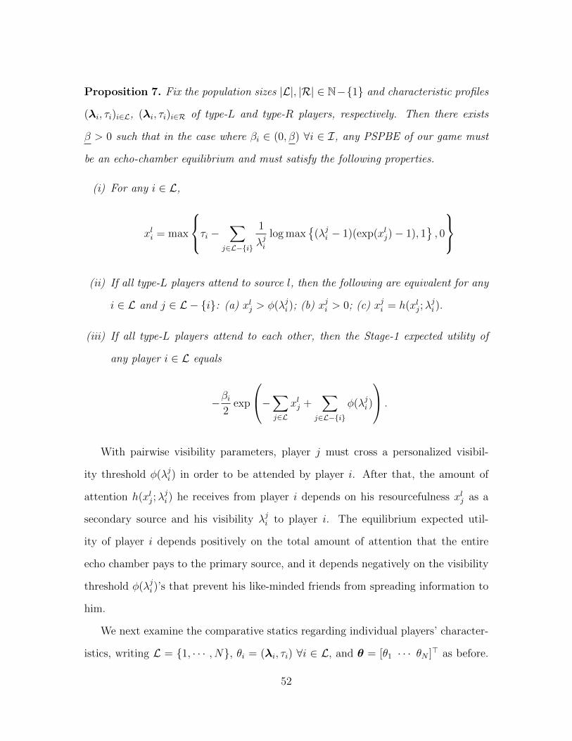
Proposition 7. Fix the population sizes |L|, |R| ∈ N−{1} and characteristic profiles

(λi, τi)i∈L, (λi, τi)i∈R of type-L and type-R players, respectively. Then there exists

β > 0 such that in the case where βi ∈ (0, β) ∀i ∈ I, any PSPBE of our game must

be an echo-chamber equilibrium and must satisfy the following properties.

(i) For any i ∈ L,

xli = max

τi − ∑j∈L−{i}

1

λjilog max

{(λji − 1)(exp(xlj)− 1), 1

}, 0

(ii) If all type-L players attend to source l, then the following are equivalent for any

i ∈ L and j ∈ L − {i}: (a) xlj > φ(λji ); (b) xji > 0; (c) xji = h(xlj;λji ).

(iii) If all type-L players attend to each other, then the Stage-1 expected utility of

any player i ∈ L equals

−βi2

exp

−∑j∈L

xlj +∑

j∈L−{i}

φ(λji )

.

With pairwise visibility parameters, player j must cross a personalized visibil-

ity threshold φ(λji ) in order to be attended by player i. After that, the amount of

attention h(xlj;λji ) he receives from player i depends on his resourcefulness xlj as a

secondary source and his visibility λji to player i. The equilibrium expected util-

ity of player i depends positively on the total amount of attention that the entire

echo chamber pays to the primary source, and it depends negatively on the visibility

threshold φ(λji )’s that prevent his like-minded friends from spreading information to

him.

We next examine the comparative statics regarding individual players’ character-

istics, writing L = {1, · · · , N}, θi = (λi, τi) ∀i ∈ L, and θ = [θ1 · · · θN ]> as before.

52

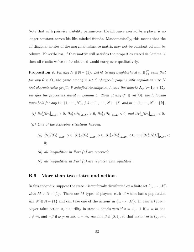
Note that with pairwise visibility parameters, the influence exerted by a player is no

longer constant across his like-minded friends. Mathematically, this means that the

off-diagonal entries of the marginal influence matrix may not be constant column by

column. Nevertheless, if that matrix still satisfies the properties stated in Lemma 3,

then all results we’ve so far obtained would carry over qualitatively.

Proposition 8. Fix any N ∈ N− {1}. Let Θ be any neighborhood in RN2

++ such that

for any θ ∈ Θ, the game among a set L of type-L players with population size N

and characteristic profile θ satisfies Assumption 1, and the matrix AN := IN + GN

satisfies the properties stated in Lemma 3. Then at any θ◦ ∈ int(Θ), the following

must hold for any i ∈ {1, · · · , N}, j, k ∈ {1, · · · , N}−{i} and m ∈ {1, · · · , N}−{k}.

(i) ∂xli/∂τi∣∣θ=θ◦

> 0, ∂xik/∂τi|θ=θ◦ > 0, ∂xlk/∂τi∣∣θ=θ◦

< 0, and ∂xkm/∂τi∣∣θ=θ◦

< 0.

(ii) One of the following situations happen:

(a) ∂xli/∂λji

∣∣θ=θ◦

> 0, ∂xik/∂λji

∣∣θ=θ◦

> 0, ∂xlk/∂λji

∣∣θ=θ◦

< 0, and ∂xkm/∂λji

∣∣θ=θ◦

<

0;

(b) all inequalities in Part (a) are reversed;

(c) all inequalities in Part (a) are replaced with equalities.

B.6 More than two states and actions

In this appendix, suppose the state ω is uniformly distributed on a finite set {1, · · · ,M}

with M ∈ N − {1}. There are M types of players, each of whom has a population

size N ∈ N − {1} and can take one of the actions in {1, · · · ,M}. In case a type-m

player takes action a, his utility in state ω equals zero if a = ω, −1 if ω = m and

a 6= m, and −β if ω 6= m and a = m. Assume β ∈ (0, 1), so that action m is type-m

53

players’ default action. Also assume that all players, regardless of their types, have

the same visibility parameter λ > 0 and bandwidth τ > 0.

There are M sources: 1-revealing, · · · , M -revealing. In state ω ∈ {1, · · · ,M},

the ω-revealing source is activated and generates news that fully reveals ω. To make

informed decisions, players attend to sources and to other players as in the baseline

model. Our solution concept is symmetric PSPBE, whereby players of the same type

adopt the same strategy. Moreover, we parameterize the attention strategy of any

type-m player by four quantities:

(i) ∆∗: the amount of attention he pays to the m-revealing source.

(ii) x∗: the amount of attention he pays to any other source.

(iii) y∗: the amount of attention he pays to each of his like-minded friends.

(iv) z∗: the amount of attention he pays to any other player.

A symmetric PSPBE of the above kind constitutes a generalized echo-chamber equi-

librium if ∆∗ = 0 and y∗ > z∗. That is, no player wastes time on learning that the

state favors his default action, and all players prioritize like-minded friends over other

players when deciding whom to pay attention to.

The next theorem proves an analog of Theorem 1: when players have sufficiently

strong preferences for taking their default actions, any symmetric PSPBE of the above

kind must be a generalized echo-chamber equilibrium, and such an equilibrium exists.

Theorem 8. For any M,N ∈ N−{1}, λ > 1/(M −1) and τ > (M −1)φ(λ(M −1)),

there exist β ∈ (0, 1) such that for any β < β, our game has a unique symmetric

PSPBE of the above kind that is also a generalized echo-chamber equilibrium.

54

B.7 Proofs

Proof of Theorem 4 In any symmetric PSPBE, either all players take their default

actions in event Ui’s, or type-L players take action R and type-R players take action

L in event Ui’s. Below we solve for the unique equilibrium of the first kind and

demonstrate that no equilibrium of the second kind exists when N is large.

For any equilibrium of the first kind, we can show, based on the arguments made in

the proof of Theorem 1, that all players must attend only to their own-biased sources

and like-minded friends at Stage 1 of the game. Then based on the arguments made in

the proof of Proposition 1, we can show that each player pays x (N) units of attention

to his own-biased source and h(x(N);λ) units of attention to each of his N − 1 like-

minded friends, where x(N) is the unique fixed point of ϕN(x) = τ − (N − 1)h(x;λ).

His Stage 1-expected utility equals −β exp (−Nx (N) + (N − 1)φ (λ)) /2.

To sustain the above outcomes on the equilibrium path, we must show that no

type-L player benefits from attending to source r and type-R players and then taking

action R in event Ui. In case a type-L player i ∈ L commits such a deviation, his best

response is to pay yji = h (x (N) ;λ) units of attention to each type-R player j ∈ R

and yri = τ − Nh(x(N);λ) units of attention to source r, where yri = ϕN(x(N)) −

h(x(N);λ) = x(N) − h(x(N);λ) → φ(λ) > 0 as N → ∞ by Lemma 4. His Stage 1-

expected utility equals − exp (−yri −Nx (N) +Nφ (λ)) /2, which, after simplifying,

becomes

− 1

2exp

(−τ +

N (τ − x (N))

N − 1−Nx (N) +Nφ (λ)

)(12)

Comparing (12) and the on-path expected utility, we find that the above deviation is

unprofitable if and only if

τ

N − 1+ φ (λ)− N

N − 1x (N) > log β.

55

Since the left-hand side of the above inequality converges to zero as N grows to

infinity by Lemma 4, it must exceed the right-hand side when N is sufficiently large.

We next argue that no equilibrium of the second kind exists when N is large. If

the contrary is true, then we can show, based on the arguments made in the proof

of Proposition 1, that on the equilibrium path, each type-L player (resp. type-R

player) pays x(N) units of attention to source r (resp. source l) and h(x(N);λ) units

of attention to each of his N − 1 like-minded friends. The Stage-1 expected utility

of any type-L player equals − exp (−Nx (N) +Nφ (λ)) /2, which falls short of what

he could earn from attending to source r and type-R players when N is large: by

committing this deviation, the player could increase his Stage 1-expected utility to

β · (12) for the reason given in the preceding paragraph.

Proof of Theorem 5 Let |L| = |R| = N ≥ 2 and (βi, λi, τi) = (β, λ, τ) ∀i ∈ I.

When β is sufficiently small, it’s efficient for players to take their default actions in

event Ui’s. Given this, the social planner’s problem becomes

maxx∈×i∈IXi

−∑i∈L

δli∏

j∈I−{i}

(δli +

(1− δlj

)δji)−∑i∈R

δri∏

j∈I−{i}

(δri +

(1− δrj

)δji).

Since the above problem has a strictly concave maximand and a compact convex

choice set, its solution is unique, and any interior solution to it must be character-

ized by first-order conditions. Consider a particular kind of interior solution that

parameterizes the attention profile of any player by four quantities:

(i) x∗ > 0: the amount of attention he pays to his own-biased source;

(ii) y∗ > 0: the amount of attention he pays to the other source;

(iii) z∗ > 0: the amount of attention he pays to each of his like-minded friends;

56

(iv) ∆∗ > 0: the amount of attention he pays to any other player.

Such a solution, if it exists, must solve the planner’s original problem, and it doesn’t

exhibit echo chambers.

The remainder of the proof provides sufficient conditions for a solution of the above

kind to exist. For ease of notation, write A for exp(−x∗)+(1− exp(−x∗)) exp(−λz∗),

B for exp(−y∗) + (1 − exp(−y∗)) exp(−λ∆∗), a for exp(x∗) − 1, b for exp(y∗) − 1, c

for exp(λz∗)− 1, and d for exp(λ∆∗)− 1. Fix any type-L player i ∈ L, and let γ > 0

denote the Lagrange multiplier associated with his bandwidth constraint, which must

be binding. The first-order conditions regarding xli, xri , x

ji , j ∈ L, and xki , i ∈ R are

δliAN−1BN +

∑j∈L−{i}

δliδlj(1− δij)AN−2BN = γ (FOCxli

)

∑j∈R

δri δrj (1− δij)AN−1BN−1 = γ (FOCxri

)

λδli(1− δlj)δjiA

N−2BN = γ (FOCxji)

and λδli(1− δlj)δjiA

N−1BN−1 = γ, (FOCxki)

and setting xli = x∗, xri = y∗, xji = z∗, and xki = ∆∗ in these FOCs yields

(λ− 1)a = Nc+ 1

Nd = λb

λa(b+ d+ 1) = Nd(a+ c+ 1)

log(a+ 1) + log(b+ 1) + N−1λ

log(c+ 1) + Nλ

log(d+ 1) = τ.

57

Solving the first three linear equations yields

b =Na

N − 1− a, c =

(λ− 1)a− 1

N, and d =

λa

N − 1− a.

Substituting these solutions into the last equation yields

log(a+ 1) + log

(Na

N − 1− a+ 1

)+N − 1

λlog

((λ− 1)a− 1

N+ 1

)+N

λlog

(λa

N − 1− a+ 1

)= τ. (13)

It remains to find conditions on (λ, τ,N) such that (13) admits a solution a(λ, τ,N)

satisfying

a(·) > 0,Na(·)

N − 1− a(·)> 0,

(λ− 1)a(·)− 1

N> 0, and

λa(·)N − 1− a(·)

> 0,

or equivalently

λ >N

N − 1and a(·) ∈

(1

λ− 1, N − 1

).

To see when a(·) ∈ (1/(λ − 1), N − 1) is satisfied, note that the left-hand side of

(13) as a function of a (i) is well-defined on (0, N − 1), (ii) is negative when a ≈ 0,

(iii) → +∞ as a → N − 1, (iv) is strictly increasing in a, and (v) is independent of

τ . Thus for any N ≥ 2 and λ > N/(N − 1), there exists a threshold τ(λ,N) such

that the solution to (13) belongs to (1/(λ − 1), N − 1) for any τ > τ(λ,N), which

completes the proof.

Proof of Theorem 6 Write {1, · · · , N} for PV , and recall that τi > φ(λi) (which

only holds if λi > 1) ∀i ∈ PV . Given this, we can simplify the system of Equation

58

(7) among members of PV to

xli = max

τi − ∑j∈PV−{i}

max{h(xlj;λj), 0

}, 0

∀i ∈ PV . (14)

Below we demonstrate that if (λi, τi) = (λ, τ) ∀i ∈ PV and if τ − (|PV|− 2)h(τ ;λ) >

φ (λ), then (14) has a unique solution xli = x(N) ∀i ∈ PV , where x(N) ∈ (φ(λ), τ) is

the unique fixed point of ϕN(x) = τ − (N − 1)h(x;λ).

Consider first the case N = 2. In that case, (14) is simply

xl1 = max{τ −max

{h(xl2;λ

), 0}, 0}

and xl2 = max{τ −max

{h(xl1;λ

), 0}, 0},

and it has a unique solution (xl1, xl2) = (x(2), x(2)). For each N ≥ 3, we fix any

pair i 6= j. Define τ = τ −∑k 6=i,j

max{h(xlk;λ

), 0}

, and note that τ ∈ (φ(λ), τ) by

assumption. Then from

xli = max{τ −max

{h(xlj;λ

), 0}, 0}

and xlj = max{τ −max

{h(xli;λ

), 0}, 0},

it follows that (xli, xlj) is the unique solution to the system of equations in the case

of N = 2 with τ replaced with τ , so it must satisfy xli = xlj ∈ (φ (λ) , τ). Repeating

the above argument for all pairs of i, j shows that xli = xlj ∈ (φ (λ) , τ) ∀i, j ∈ PV .

Simplifying (14) accordingly yields xli = ϕN(xli)

and, hence, xli = x (N) ∀i ∈ PV .

Proof of Proposition 5 The proof closely parallels that of Theorems 1-3 and hence

is omitted.

59

Proof of Theorem 7 Write {1, · · · , N} for PV and define yi = xli − τ i and ∆τi =

τ i − τ i for each i ∈ PV . By definition, any i ∈ PV must satisfy τ i > τ i > φ(λi) and,

hence, λi > 1. Given this, we can simplify the best response function of any i ∈ PV :

xli = max

τ i − ∑j∈PV−{i}

1

λilog max{(λj − 1)(exp(xlj)− 1), 1}, τ i

to:

yi = max

∆τi −∑

j∈PV−{i}

h(ylj + τ j;λj), 0

.

For each y = [y1 · · · yN ]> ∈ Y := ×Ni=1[0,∆τi], define F (y) as the N -vector whose

ith entry is given by yi +∑

j∈PV−{i} h(ylj + τ j;λj) − ∆τi. Note that the function

F : Y → RN is strongly monotone,10 because for any y,y′ ∈ Y :

(y − y′)>(F (y)− F (y′))

=N∑i=1

(yi − y′i)2 −N∑i=1

∑j 6=i

(yi − y′i)[hx(yj;λj)− hx(y′j;λj)]

≥ ‖y − y′‖2 − gN∑i=1

∑j 6=i

|yi − y′i||yj − y′j| (∵ hx(·; ·) ∈ (0, g))

≥ [1− (N − 1)g]︸ ︷︷ ︸>0 by assumption

‖y − y′‖2.

Then from Proposition 1 of Naghizadeh and Liu (2017), it follows that the game

among members of PV has a unique equilibrium.

Proof of Proposition 7 The proof closely parallels that of Theorems 1 and 2 and

hence is omitted for brevity.

10A function f : K → Rn defined on a closed convex set K ⊂ Rn is strongly monotone if thereexists c > 0 such that (x− y)>(F (x)− F (y)) > c‖x− y‖2 ∀x,y ∈ K.

60

Proof of Proposition 8 Write {1, · · · , N} for L. Under the assumption stated in

Proposition 8, the following must hold ∀i ∈ {1, · · · , N} and j ∈ {1, · · · , N}−{i}: (i)

xli = τi −∑

j∈L−{i}

h(xlj;λji ) (15)

and xji = h(xlj;λji ), (16)

(ii) xlj > φ(λji ) and, hence, hx(xlj;λ

ji ) := [GN ]i,j ∈ (0, 1); (iii) AN := IN +GN satisfies

the properties stated in Lemma 3.

Part (i): The proof is the exact same as that of Theorem 3(i) and hence is omitted.

Part (ii): We only prove the result for i = 1 and j = 2. Differentiating the system of

Equation (15) among i ∈ {1, · · · , N} with respect to λ21 yields

∇λ21xl = κ21A

−1N [1 0 · · · 0]> ,

where xl := [xl1 · · · xlN ]>, and κ21 := −hλ(xl2;λ21) has an ambiguous sign in general.

Then from the assumption that[A−1N

]1,1> 0 and

[A−1N

]k,1< 0 ∀k 6= 1, it follows that

sgn

(∂xl1∂λ21

)= sgn

(κ21[A−1N

]1,1

)= sgn

(κ21)

and

sgn

(∂xlk∂λ21

)= sgn

(κ21[A−1N

]k,1

)= sgn

(−κ21

)∀k 6= 1.

The second result and Equation (16) together imply that

sgn

(∂x1k∂λ21

)= sgn

(hx(x

l1;λ

1k)∂xl1∂λ21

)= sgn

(κ21)∀k 6= 1

61

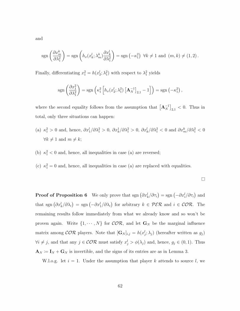
and

sgn

(∂xkm∂λ21

)= sgn

(hx(x

lk;λ

km)∂xlk∂λ21

)= sgn

(−κ21

)∀k 6= 1 and (m, k) 6= (1, 2) .

Finally, differentiating x21 = h(xl2;λ21) with respect to λ21 yields

sgn

(∂x21∂λ21

)= sgn

(κ21

[hx(x

l2;λ

21)[A−1N

]2,1− 1])

= sgn(−κ21

),

where the second equality follows from the assumption that[A−1N

]2,1

< 0. Thus in

total, only three situations can happen:

(a) κ21 > 0 and, hence, ∂xl1/∂λ21 > 0, ∂x1k/∂λ

21 > 0, ∂xlk/∂λ

21 < 0 and ∂xkm/∂λ

21 < 0

∀k 6= 1 and m 6= k;

(b) κ21 < 0 and, hence, all inequalities in case (a) are reversed;

(c) κ21 = 0 and, hence, all inequalities in case (a) are replaced with equalities.

Proof of Proposition 6 We only prove that sgn(∂xlk/∂τi

)= sgn

(−∂xli/∂τi

)and

that sgn(∂xlk/∂λi

)= sgn

(−∂xl1/∂λi

)for arbitrary k ∈ PER and i ∈ COR. The

remaining results follow immediately from what we already know and so won’t be

proven again. Write {1, · · · , N} for COR, and let GN be the marginal influence

matrix among COR players. Note that [GN ]i,j = h(xlj;λj) (hereafter written as gj)

∀i 6= j, and that any j ∈ COR must satisfy xlj > φ(λj) and, hence, gj ∈ (0, 1). Thus

AN := IN + GN is invertible, and the signs of its entries are as in Lemma 3.

W.l.o.g. let i = 1. Under the assumption that player k attends to source l, we

62

must have

xlk = τk −N∑j=1

1

λjlog[(λj − 1)(exp(xlj)− 1)

]. (17)

Differentiating both sides of Equation (17) with respect to τ1 yields

∂xlk∂τ1

=N∑j=1

−gj∂xlj∂τ1

,

and simplifying this result using ∇τ1 [xl1 · · · xlN ]> = A−1N [1 0 · · · 0]> (as shown in the

proof of Theorem 3) and doing a lot of algebra yield

∂xlk∂τ1

= (1− g1)∂xl1∂τ1− 1.

Then from ∂xl1/∂τ1 > 0 (Theorem 3), it follows that sgn(∂xlk/∂τ1) = sgn(−∂xl1/∂τ1)

if and only if ∂xl1/∂τ1 < 1/ (1− g1). To establish the last inequality, recall that

∂xl1/∂τ1 =[A−1N

]1,1

, whose expression is given by Equation (4). Tedious but straight-

forward algebra shows that

[A−1N

]1,1− 1

1− g1=

−g1det (AN) (1− g1)

N∏j=2

(1− gj) < 0,

which completes the proof.

Meanwhile, differentiating both sides of Equation (17) with respect to λ1 yields

∂xlk∂λ1

= −N∑j=1

gj∂xlj∂λ1

+ κ

where κ = −hλ(xl1;λ1). Simplifying this result using∇λ1 [xl1 · · · xlN ]> = κA−1N [0 1 · · · 1]>

63

(as shown in the proof of Theorem 3) and doing a lot of algebra yield

∂xlk∂λ1

= (1− g1)∂xl1∂λ1

+ κ

= κ

((1− g1)

N∑j=2

[A−1N

]1,j

+ 1

)

=κ

det (AN)

N∏j=2

(1− gj) .

Then from sgn(∂xl1/∂λ1

)= sgn (−κ) (as shown in the proof of Theorem 3), it follows

that sgn(∂xlk/∂λ1

)= sgn

(−∂xl1/∂λ1

), which completes the proof.

Proof of Theorem 8 In the setting laid out in Appendix B.6, the set of the parties

that any player i can attend to is Ci = {1-rev, · · · ,m-rev} ∪ I − {i}, and the set Xi

of feasible attention strategies for him must be modified accordingly. When β is

sufficiently small, we note, for the reason given in the proof of Theorem 1, that all

players must take their default actions in case they remain uninformed of the state

at Stage 4 of the game. Given this, we can formulate the Stage 1-problem faced by

any type-m player as follows:

maxxi∈Xi

− β

M

∑ω 6=m

δω−revealingi

∏j∈I−{i}

(δω−revealingj +

(1− δω−revealingj

)δji

).

Using the parameterization specified in Appendix B.6 and solving, we obtain ∆∗ = 0,

(M − 1)x∗ + (N − 1)y∗ + (M − 1)Nz∗ = τ , y∗ = g1 (x∗) and z∗ = g2 (x∗), where

g1 (x) :=1

λlog max {(λ (M − 1)− 1) (exp (x)− 1) , 1}

and g2 (x) :=1

λlog max {(λ (M − 2)− 1) (exp (x)− 1) , 1} .

64

Thus x∗ is the unique fixed point of 1M−1 [τ − (N − 1) g1 (x)− (M − 1)Ng2 (x)], and

the following are equivalent: (i) y∗ > 0; (ii) y∗ > z∗; (iii) λ > 1/(1 − M) and

τ > (M − 1)φ (λ (M − 1)).

65

C Figures

Figure 1: A and B represent equilibrium (xl1, xl2)’s when λ1 = 1.5 and 2, respectively:

λ2 = 1.5, τ1 = τ2 = 3.

Figure 2: A and B represent equilibrium (xl1, xl2)’s when λ1 = 1.5 and 4, respectively:

λ2 = 1.5, τ1 = τ2 = 3.

66

References

Adamic, L. A., and N. S. Glance (2005): “The political blogosphere and the 2004

U.S. election: Divided they blog,” Proceedings of the 3rd International Workshop

on Link Discovery, August 2005, 36-43.

Allcott, H., L. Braghieri, S. Eichmeyer, and M. Gentzkow. (2020): “The

welfare effects of social media,” American Economic Review, 110(3), 629-676.

Barbera, P. (2020): “Social Media, Echo Chambers, and Political Polarization,”

in Social Media and Democracy: The State of the Field, ed. by N. Persily., and J.

Tucker.. Cambridge University Press.

Baccara, M., and L. Yariv. (2013): “Homophily in peer groups,” American

Economic Journal: Microeconomics, 5(3), 69-96.

Bakshy, E., S. Messing, and A. Lada. (2015): “Exposure to ideologically diverse

news and opinion on Facebook,” Science, 348(6239), 1130-1132.

Bala, V., and S. Goyal. (2000): “A noncooperative model of network formation,”

Econometrica, 68(5), 1181-1229.

Balsamo, D., V. Gelardi, C. Han, D. Rama, A. Samantray, C. Zucca, and

M. Starnini. (2019): “Inside the echo chamber: Disentangling network dynamics

from polarization,” Working paper (accessible at arXiv:1906.09076v2 [physics. soc-

ph]).

Baum, M., and A. S. Jamison. (2006): “The Oprah effect: How soft news helps

inattentive citizens vote consistently,” Journal of Politics, 68(4), 946-959.

67

Bloch, F., G. Gemange, and R. Kranton. (2018): “Rumors and social net-

works,” International Economic Review, 59(2), 421-448.

Bramoulle, Y., R. Kranton, and M. D’Amours. (2014): “Strategic interaction

and networks,” American Economic Review, 104(3), 898-930.

Calvert, R. L. (1985): “The value of biased information: A rational choice model

of political advice,” Journal of Politics, 47(2), 530-555.

Che, Y-K., and K. Mierendorff. (2019): “Optimal dynamic allocation of atten-

tion,” American Economic Review, 109(8), 2993-3029.

Chiang, C-F., and B. Knight. (2011): “Media bias and influence: evidence from

newspaper endorsements,” Review of Economic Studies, 78(3), 795-820.

Cossard, A., G. De Francisci Morales, K. Kalimeri, Y. Mejova, D.

Paolotti, and M. Starnini. (2020): “Falling into the echo chamber: the Italian

vaccination debate on Twitter,” Working paper (accessible at arXiv:2003.11906v1

[cs.CY]).

Del Vicario M., A. Bessi, F. Zollo, F. Petroni, A. Scala, G. Caldarel-

lia, H. E. Stanley, and W. Quattrociocchi. (2016): “The spreading of

misinformation online,” Proceedings of National Academy of Sciences, 113(3), 554-

559.

DellaVigna, S., and M. Gentzkow. (2010): “Persuasion: Empirical evidence,”

Annual Review of Economics, 2, 643-669.

Denti, T. (2015): “Unrestricted information acquisition,” Working paper.

Dessein, W., A. Galeotti, and T. Santos. (2016): “Rational inattention and

organizational focus,” American Economic Review, 106(6), 1522-1536.

68

Farrell H., and D. W. Drezner. (2008): “The power and politics of blogs,”

Public Choice, 134, 15-30.

Flaxman, S., S. Goel, and J. M. Rao. (2016): “Filter bubbles, echo chambers

and online news consumption,” Public Opinion Quarterly, 80(S1), 298-320.

Furst, S. (2020): “In the service of good journalism and audience interests? How

audience metrics affect news quality,” Media and Communication, 8(3), 270-280.

Galeotti, A., C. Ghiglino, and F. Squintani. (2013): “Strategic information

transmission networks,” Journal of Economic Theory, 148, 1751-1769.

Galeotti, A., and S. Goyal. (2010): “The law of the few,” American Economic

Review, 100(4), 1468-1492.

Ho, D. E., and K. M. Quinn. (2009): “Viewpoint diversity and media consolida-

tion: An empirical study,” Stanford Law Review, 61(4), 781-868.

Hu, L., A. Li, and I. Segal. (2019): “The politics of personalized news aggrega-

tion,” Working paper (accessible at arXiv:1910.11405 [econ.GN]).

Jackson, M. O. (2014): “Networks in the understanding of economic behaviors,”

Journal of Economic Perspectives, 28(4), 3-22.

Kinateder, M., and L. P. Merlino. (2017): “Public goods in endogenous net-

works,” American Economic Journal: Microeconomics, 9(3), 187-212.

Lazarsfeld. P. F., B. Berelson, and H. Gaudet. (1948): The People’s Choice:

How the Voter Makes Up His Mind in a Presidential Campaign, New York, NY:

Columbia University Press.

69

Levy, G., and R. Razin. (2019): “Echo chambers and their effects on economic

and political outcomes,” Annual Review of Economics, 11, 303-328.

Lu, Y., P. Zhang, Y. Cao, Y. Hua, and L. Guo. (2014): “On the frequency

distribution of retweets,” Procedia Computer Science, 31, 747-753.

Matsa, K. E., and K. Lu. (2016): “10 Facts about the changing digital news

landscape,” Pew Research Center, September 14.

Meng, D. (2021): “Learning from like-minded people,” Games and Economic Be-

havior, 126, 231-250.

Mosleh, M., C. Martel, D. Eckles, and D. G. Rand. (2021) “Shared parti-

sanship dramatically increases social tie formation in a Twitter field experiment,”

Proceedings of National Academy of Sciences, 118(7), e2022761118.

Naghizadeh, P., and M. Liu. (2017): “On the uniqueness and stability of equilib-

ria of network games,” 2017 55th Annual Allerton Conference on Communication,

Control, and Computing (Allerton), Monticello, IL, 2017, 280-286.

Neda, Z., L. Varga, and T.S. Biro. (2017): “Science and Facebook: The same

popularity law!,” PLOS One, 12(7), e0179656.

Newman, N. (2009): “The rise of social media and its impact on mainstream jour-

nalism,” Working paper, Reuters Institute for the Study of Journalism.

Pariser, E. (2011): The Filter Bubble: How the New Personalized Web Is Changing

What We Read and How We Think, New York, NY: Penguin Press.

Prior, M. (2007): Post-Broadcast Democracy: How Media Choice Increases Inequal-

ity in Political Involvement and Polarizes Elections, New York, NY: Cambridge

University Press.

70

Romm, T. (2021): “ Facebook, Twitter could face punishing regulation for their role

in U.S. Capitol riot, Democrats say,” The Washington Post, January 8.

Sethi, R., and M. Yildiz (2016): “Communication with unknown perspectives,”

Econometrica, 84(6), 2029-2069.

Sims, C. A. (1998): “Stickiness,” Carnegie-Rochester Conference Series on Public

Policy, 49(1), 317-356.

——— (2003): “Implications of rational inattention,” Journal of Monetary Eco-

nomics, 50(3), 665-690.

Smith, M. (2016): “So you think you chose to read this article?,” BBC News, July

21.

Suen, W. (2004): “The self-perpetuation of biased beliefs,” The Economic Journal,

114, 377-396.

Winter, S., and G. Neubaum. (2016): “Examining characteristics of opinion

leaders in social media: A motivational approach,” Social Media+Society, 2(3),

1-12.

Zhong, W. (2017): “Optimal dynamic information acquisition,” Working Paper.

71