A Random Forest Guided Tour

Gerard BiauSorbonne Universites, UPMC Univ Paris 06, F-75005, Paris, France& Institut Universitaire de Francegerard.biau@upmc.fr

Erwan ScornetSorbonne Universites, UPMC Univ Paris 06, F-75005, Paris, Franceerwan.scornet@upmc.fr

Abstract

The random forest algorithm, proposed by L. Breiman in 2001, hasbeen extremely successful as a general purpose classification and re-gression method. The approach, which combines several randomizeddecision trees and aggregates their predictions by averaging, has shownexcellent performance in settings where the number of variables ismuch larger than the number of observations. Moreover, it is versa-tile enough to be applied to large-scale problems, is easily adapted tovarious ad-hoc learning tasks, and returns measures of variable im-portance. The present article reviews the most recent theoretical andmethodological developments for random forests. Emphasis is placedon the mathematical forces driving the algorithm, with special atten-tion given to the selection of parameters, the resampling mechanism,and variable importance measures. This review is intended to providenon-experts easy access to the main ideas.

Index Terms — Random forests, randomization, resampling, param-eter tuning, variable importance.

2010 Mathematics Subject Classification: 62G05, 62G20.

1 Introduction

To take advantage of the sheer size of modern data sets, we now need learn-ing algorithms that scale with the volume of information, while maintainingsufficient statistical efficiency. Random forests, devised by L. Breiman inthe early 2000s (Breiman, 2001), are part of the list of the most successfulmethods currently available to handle data in these cases. This supervised

1

learning procedure, influenced by the early work of Amit and Geman (1997),Ho (1998), and Dietterich (2000), operates according to the simple but ef-fective “divide and conquer” principle: sample small fractions of the data,grow a randomized tree predictor on each small piece, then paste (aggregate)these predictors together.

What has greatly contributed to the popularity of forests is the fact thatthey can be applied to a wide range of prediction problems and have fewparameters to tune. Aside from being simple to use, the method is generallyrecognized for its accuracy and its ability to deal with small sample sizes andhigh-dimensional feature spaces. At the same time, it is easily parallelizableand has therefore the potential to deal with large real-life systems. Thecorresponding R package randomForest can be freely downloaded on theCRAN website (http://www.r-project.org), while a MapReduce (Jeffrey andSanja, 2008) open source implementation called Partial Decision Forests isavailable on the Apache Mahout website at https://mahout.apache.org. Thisallows the building of forests using large data sets as long as each partitioncan be loaded into memory.

The random forest methodology has been successfully involved in variouspractical problems, including a data science hackathon on air quality pre-diction (http://www.kaggle.com/c/dsg-hackathon), chemoinformatics (Svet-nik et al., 2003), ecology (Prasad et al., 2006; Cutler et al., 2007), 3Dobject recognition (Shotton et al., 2011) and bioinformatics (Dıaz-Uriarteand de Andres, 2006), just to name a few. J. Howard (Kaggle) and M.Bowles (Biomatica) claim in Howard and Bowles (2012) that ensembles ofdecision trees—often known as “random forests”—have been the most suc-cessful general-purpose algorithm in modern times, while H. Varian, ChiefEconomist at Google, advocates in Varian (2014) the use of random forestsin econometrics.

On the theoretical side, the story of random forests is less conclusive and,despite their extensive use, little is known about the mathematical propertiesof the method. The most celebrated theoretical result is that of Breiman(2001), which offers an upper bound on the generalization error of forests interms of correlation and strength of the individual trees. This was followedby a technical note (Breiman, 2004), which focuses on a stylized versionof the original algorithm (see also Breiman, 2000a,b). A critical step wassubsequently taken by Lin and Jeon (2006), who highlighted an interestingconnection between random forests and a particular class of nearest neighborpredictors, further developed by Biau and Devroye (2010). In recent years,various theoretical studies have been performed (e.g., Meinshausen, 2006;

2

Biau et al., 2008; Ishwaran and Kogalur, 2010; Biau, 2012; Genuer, 2012;Zhu et al., 2012), analyzing more elaborate models and moving ever closer tothe practical situation. Recent attempts towards narrowing the gap betweentheory and practice include that of Denil et al. (2013), who prove the firstconsistency result for online random forests, and Mentch and Hooker (2014b)and Wager (2014), who study the asymptotic distribution of forests.

The difficulty in properly analyzing random forests can be explained by theblack-box flavor of the method, which is indeed a subtle combination of dif-ferent components. Among the forests’ essential ingredients, both bagging(Breiman, 1996) and the Classification And Regression Trees (CART)-splitcriterion (Breiman et al., 1984) play critical roles. Bagging (a contractionof bootstrap-aggregating) is a general aggregation scheme, which generatesbootstrap samples from the original data set, constructs a predictor fromeach sample, and decides by averaging. It is one of the most effective compu-tationally intensive procedures to improve on unstable estimates, especiallyfor large, high-dimensional data sets, where finding a good model in one stepis impossible because of the complexity and scale of the problem (Buhlmannand Yu, 2002; Kleiner et al., 2012; Wager et al., 2013). As for the CART-splitcriterion, it originates from the influential CART algorithm of Breiman et al.(1984), and is used in the construction of the individual trees to choose thebest cuts perpendicular to the axes. At each node of each tree, the best cut isselected by optimizing the CART-split criterion, based on the so-called Giniimpurity (for classification) or the prediction squared error (for regression).

However, while bagging and the CART-splitting scheme play key roles in therandom forest mechanism, both are difficult to analyze with rigorous math-ematics, thereby explaining why theoretical studies have so far consideredsimplified versions of the original procedure. This is often done by simplyignoring the bagging step and/or replacing the CART-split selection by amore elementary cut protocol. As well as this, in Breiman’s (2001) forests,each leaf (that is, a terminal node) of individual trees contains a fixed pre-specified number of observations (this parameter is usually chosen between 1and 5). Disregarding the subtle combination of all these components, mostauthors have focused on stylized, data-independent procedures, thus creatinga gap between theory and practice.

The goal of this survey is to embark the reader on a guided tour of ran-dom forests. We focus on the theory behind the algorithm, trying to give anoverview of major theoretical approaches while discussing their inherent prosand cons. For a more methodological review covering applied aspects of ran-dom forests, we refer to the surveys by Criminisi et al. (2011) and Boulesteix

3

et al. (2012). We start by gently introducing the mathematical context inSection 2 and describe in full detail Breiman’s (2001) original algorithm. Sec-tion 3 focuses on the theory for a simplified forest model called purely randomforests, and emphasizes the connections between forests, nearest neighbor es-timates and kernel methods. Section 4 provides some elements of theoryabout resampling mechanisms, the splitting criterion and the mathematicalforces at work in Breiman’s approach. Section 5 is devoted to the theo-retical aspects of associated variable selection procedures. Lastly, Section6 discusses various extensions to random forests including online learning,survival analysis and clustering problems.

2 The random forest estimate

2.1 Basic principles

As mentioned above, the random forest mechanism is versatile enough todeal with both supervised classification and regression tasks. However, tokeep things simple, we focus in this introduction on regression analysis, andonly briefly survey the classification case.

Our goal in this section is to provide a concise but mathematically precisepresentation of the algorithm for building a random forest. The generalframework is nonparametric regression estimation, in which an input ran-dom vector X ∈ [0, 1]p is observed, and the goal is to predict the squareintegrable random response Y ∈ R by estimating the regression functionm(x) = E[Y |X = x]. With this aim in mind, we assume we are given atraining sample Dn = (X1, Y1), . . . , (Xn, Yn) of independent random vari-ables distributed the same as the independent prototype pair (X, Y ). Thegoal is to use the data set Dn to construct an estimate mn : [0, 1]p → R ofthe function m. In this respect, we say that the regression function estimatemn is (mean squared error) consistent if E[mn(X)−m(X)]2 → 0 as n→∞(the expectation is evaluated over X and the sample Dn).

A random forest is a predictor consisting of a collection of M randomizedregression trees. For the j-th tree in the family, the predicted value at thequery point x is denoted by mn(x; Θj,Dn), where Θ1, . . . ,ΘM are indepen-dent random variables, distributed the same as a generic random variable Θand independent of Dn. In practice, the variable Θ is used to resample thetraining set prior to the growing of individual trees and to select the suc-cessive directions for splitting—more precise definitions will be given later.

4

At this stage, we note that the trees are combined to form the (finite) forestestimate

mM,n(x; Θ1, . . . ,ΘM ,Dn) =1

M

M∑j=1

mn(x; Θj,Dn). (1)

In the R package randomForest, the default value of M (the number oftrees in the forest) is ntree = 500. Since M may be chosen arbitrarilylarge (limited only by available computing resources), it makes sense, froma modeling point of view, to let M tends to infinity, and consider instead of(1) the (infinite) forest estimate

m∞,n(x;Dn) = EΘ [mn(x; Θ,Dn)] .

In this definition, EΘ denotes the expectation with respect to the randomparameter Θ, conditional on Dn. In fact, the operation “M →∞” is justifiedby the law of large numbers, which asserts that almost surely, conditional onDn,

limM→∞

mM,n(x; Θ1, . . . ,ΘM ,Dn) = m∞,n(x;Dn)

(see for instance Breiman, 2001, and Scornet, 2014, for more information onthis limit calculation). In the following, to lighten notation we will simplywrite m∞,n(x) instead of m∞,n(x; Dn).

Classification. In the (binary) supervised classification problem (Devroyeet al., 1996), the random response Y takes values in {0, 1} and, given X, onehas to guess the value of Y . A classifier or classification rule mn is a Borelmeasurable function of x and Dn that attempts to estimate the label Y fromx and Dn. In this framework, one says that the classifier mn is consistent ifits conditional probability of error

L(mn) = P[mn(X) 6= Y |Dn]

satisfieslimn→∞

EL(mn) = L?,

where L? is the error of the optimal—but unknown—Bayes classifier:

m?(x) =

{1 if P[Y = 1|X = x] > P[Y = 0|X = x]0 otherwise.

In the classification situation, the random forest classifier is obtained via amajority vote among the classification trees, that is,

mM,n(x; Θ1, . . . ,ΘM ,Dn) =

{1 if 1

M

∑Mj=1mn(x; Θj,Dn) > 1/2

0 otherwise.

5

2.2 Algorithm

We now provide some insight on how the individual trees are constructed andhow randomness kicks in. In Breiman’s (2001) original forests, each node ofa single tree is associated with a hyperrectangular cell. At each step of thetree construction, the collection of cells forms a partition of [0, 1]p. The rootof the tree is [0, 1]p itself, and the terminal nodes (or leaves), taken together,form a partition of [0, 1]p. If a leaf represents region A, then the regressiontree outputs on A the average of all Yi for which the corresponding Xi falls inA. Algorithm 1 describes in full detail how to compute a forest’s prediction.

Algorithm 1 may seem a bit complicated at first sight, but the underlyingideas are simple. We start by noticing that this algorithm has three importantparameters:

1. an ∈ {1, . . . , n}: the number of sampled data points in each tree;

2. mtry ∈ {1, . . . , p}: the number of possible directions for splitting ateach node of each tree;

3. nodesize ∈ {1, . . . , n}: the number of examples in each cell belowwhich the cell is not split.

The algorithm works by growing M different (randomized) trees as follows.Prior to the construction of each tree, an observations are drawn at randomwith replacement from the original data set; then, at each cell of each tree,a split is performed by maximizing the CART-criterion (see below); lastly,construction of individual trees is stopped when each cell contains less thannodesize points. By default in the regression mode, the parameter mtry isset to p/3, an is set to n, and nodesize is set to 5. The role and influenceof these three parameters on the accuracy of the method will be thoroughlydiscussed in the next section.

We still have to describe how the CART-split criterion operates. With thisaim in mind, we let A be a generic cell and denote by Nn(A) the numberof data points falling in A. A cut in A is a pair (j, z), where j is somevalue (dimension) from {1, . . . , p} and z the position of the cut along thej-th coordinate, within the limits of A. Let CA be the set of all such possiblecuts in A. Then, with the notation Xi = (X

(1)i , . . . ,X

(p)i ), for any (j, z) ∈ CA,

the CART-split criterion takes the form

6

Algorithm 1: Breiman’s random forest predicted value at x.

Input: Training set Dn, number of trees M > 0, an ∈ {1, . . . , n},mtry ∈ {1, . . . , p}, nodesize ∈ {1, . . . , n}, and x ∈ [0, 1]p.

Output: Prediction of the random forest at x.1 for j = 1, . . . ,M do2 Select an points, with replacement, uniformly in Dn.3 Set P0 = {[0, 1]p} the partition associated with the root of the tree.4 For all 1 ≤ ` ≤ an, set P` = ∅.5 Set nnodes = 1 and level = 0.6 while nnodes < an do7 if Plevel = ∅ then8 level = level + 19 else

10 Let A be the first element in Plevel.11 if A contains less than nodesize points then12 Plevel ← Plevel\{A}13 Plevel+1 ← Plevel+1 ∪ {A}14 else15 Select uniformly, without replacement, a subset

Mtry ⊂ {1, . . . , p} of cardinality mtry.16 Select the best split in A by optimizing the CART-split

criterion along the coordinates in Mtry (see text for details).17 Cut the cell A according to the best split. Call AL and AR

the two resulting cells.18 Plevel ← Plevel\{A}19 Plevel+1 ← Plevel+1 ∪ {AL} ∪ {AR}20 nnodes = nnodes + 1

21 end

22 end

23 end24 Compute the predicted value mn(x; Θj,Dn) at x equal to the average of

the Yi falling in the cell of x in partition Plevel ∪ Plevel+1.25 end26 Compute the random forest estimate mM,n(x; Θ1, . . . ,ΘM ,Dn) at the query

point x according to (1).

7

Lreg,n(j, z) =1

Nn(A)

n∑i=1

(Yi − YA)21Xi∈A

− 1

Nn(A)

n∑i=1

(Yi − YAL1X

(j)i <z− YAR

1X

(j)i ≥z

)21Xi∈A, (2)

where AL = {x ∈ A : x(j) < z}, AR = {x ∈ A : x(j) ≥ z}, and YA (resp.,YAL

, YAR) is the average of the Yi belonging to A (resp., AL, AR), with the

convention 0/0 = 0. For each cell A, the best cut (j?n, z?n) is selected by

maximizing Ln(j, z) over Mtry and CA; that is,

(j?n, z?n) ∈ arg max

j∈Mtry

(j,z)∈CA

Ln(j, z).

(To remove some of the ties in the argmax, the best cut is always performedin the middle of two consecutive data points.)

Thus, at each cell of each tree, the algorithm chooses uniformly at randommtry coordinates in {1, . . . , p}, evaluates criterion (2) over all possible cutsin the mtry directions, and returns the best one. The quality measure (2) isthe criterion used in the most influential CART algorithm of Breiman et al.(1984). This criterion measures the (renormalized) difference between theempirical variance in the node before and after a cut is performed—the onlydifference here is that it is evaluated over a subsetMtry of randomly selectedcoordinates, and not over the whole range {1, . . . , p}. However, contraryto the CART algorithm, the individual trees are not pruned, and the finalcells have a cardinality that does not exceed nodesize. Also, each tree isconstructed on a subset of an examples picked within the initial sample, noton the whole sample Dn. When an = n, the algorithm runs in bootstrapmode, whereas an < n corresponds to subsampling (with replacement). Lastbut not least, the process is repeated M (a large number) times.

Classification. In the classification case, if a leaf represents region A, thena randomized tree classifier takes the simple form

mn(x; Θj,Dn) =

{1 if

∑ni=1 1Xi∈A,Yi=1 >

∑ni=1 1Xi∈A,Yi=0, x ∈ A

0 otherwise.

That is, in each leaf, a majority vote is taken over all (Xi, Yi) for whichXi is in the same region. Ties are broken, by convention, in favor of class0. Algorithm 1 can be easily adapted to do classification by modifying the

8

CART-split criterion for the binary setting. For any cell A, let p0,n(A) (resp.,p1,n(A)) be the empirical probability that a data point with label 0 (resp.label 1) falls into A. Then, for any (j, z) ∈ CA, the classification CART-splitcriterion takes the form

Lclass,n(j, z) = p0,n(A)p1,n(A)− Nn(AL)

Nn(A)× p0,n(AL)p1,n(AL)

− Nn(AR)

Nn(A)× p0,n(AR)p1,n(AR). (3)

This criterion is based on the so-called Gini impurity measure 2p0,n(A)p1,n(A)(Breiman et al., 1984), which has a simple interpretation. Instead of usingthe majority vote to classify a data point that falls in cell A, one can usethe rule that assigns an observation, selected at random from the node, tolabel ` with probability p`,n(A), for j ∈ {0, 1}. The estimated probabilitythat the item has actually label ` is p`,n(A). Therefore the estimated prob-ability of misclassification under this rule is the Gini index 2p1,n(A)p2,n(A).When dealing with classification problems, it is usually recommended to setnodesize = 1 and mtry =

√p (see, e.g., Liaw and Wiener, 2002).

2.3 Parameter tuning

Literature focusing on tuning the parameters M , mtry, nodesize and an isunfortunately rare, with the notable exception of Dıaz-Uriarte and de Andres(2006), Bernard et al. (2008), and Genuer et al. (2010). It is easy to see thatthe forest’s variance decreases as M grows. Thus, more accurate predictionsare likely to be obtained by choosing a large number of trees. It is interestingto note that picking a large M does not lead to overfitting, since finite forestsconverge to infinite ones (Breiman, 2001). However, the computational costfor inducing a forest increases linearly with M , so a good choice results froma trade-off between computational complexity (M should not be too large forthe computations to finish in a reasonable time) and accuracy (M must belarge enough for predictions to be stable). In this respect, Dıaz-Uriarte andde Andres (2006) argue that the value of M is irrelevant (provided that M islarge enough) in a prediction problem involving microarray data sets, wherethe aim is to classify patients according to their genetic profiles (typically,less than one hundred patients for several thousand genes). For more detailswe refer the reader to Genuer et al. (2010), who offer a thorough discussionon the choice of this parameter in various regression problems. Another in-teresting and related approach is by Latinne et al. (2001), who propose a

9

simple procedure that determines a priori a minimum number of tree esti-mates to combine in order to obtain a prediction accuracy level similar tothat obtained with a larger forest. Their experimental results show that it ispossible to significantly limit the number of trees.

In the R package randomForest, the default value of the parameter nodesizeis 1 for classification and 5 for regression. These values are often reportedto be good choices (e.g., Dıaz-Uriarte and de Andres, 2006), despite the factthat this is not supported by solid theory. The effect of mtry has been thor-oughly investigated in Dıaz-Uriarte and de Andres (2006), who show thatthis parameter has a little impact on the performance of the method, thoughlarger values may be associated with a reduction in the predictive perfor-mance. On the other hand, Genuer et al. (2010) claim that the default valueof mtry is either optimal or too small. Therefore, a conservative approach isto take mtry as large as possible (limited by available computing resources)and set mtry = p (recall that p is the dimension of the Xi). A data-drivenchoice of mtry is implemented in the algorithm Forest-RK of Bernard et al.(2008).

3 Simplified models and local averaging esti-

mates

3.1 Simplified models

Despite their widespread use, a gap remains between the theoretical under-standing of random forests and their practical performance. This algorithm,which relies on complex data-dependent mechanisms, is difficult to analyzeand its basic mathematical properties are still not well understood.

This state of affairs has led to polarization between theoretical and empiricalcontributions to the literature. Empirically focused papers describe elabo-rate extensions to the basic random forest framework, adding domain-specificrefinements that push the state of the art in performance, but come with noclear guarantees. In contrast, most theoretical papers focus on simplifica-tions or stylized versions of the standard algorithm, where the mathematicalanalysis is more tractable.

A basic framework to assess the theoretical properties of forests involvesmodels that are calibrated independently of the training set Dn. This fam-ily of simplified models is often called purely random forests. A widespread

10

example is the centered forest, whose principle is as follows: (i) there is nobootstrap step; (ii) at each node of each individual tree, a coordinate is uni-formly chosen in {1, . . . , p}; and (iii) a split is performed at the center of thecell along the selected coordinate. The operations (ii)-(iii) are recursivelyrepeated k times, where k ∈ N is a parameter of the algorithm. The pro-cedure stops when a full binary tree with k levels is reached, so that eachtree ends up with exactly 2k leaves. The parameter k acts as a smoothingparameter that controls the size of the terminal cells (see Figure 1 for anexample in two dimensions). It should be chosen large enough in order todetect local changes in the distribution, but not too much to guarantee aneffective averaging process in the leaves. In uniform random forests, a variantof centered forests, cuts are performed uniformly at random over the range ofthe selected coordinate, not at the center. Modulo some minor modifications,their analysis is similar.

5,56,2

7,1

6,8 5,7

5,7

4,9

5,3

6,0

5,815,1

16,2

14,8

16,9

17,118

Figure 1: A centered tree at level 2.

The centered forest rule was formally analyzed in Biau et al. (2008) andScornet (2014), who proved that the method is consistent (both for classifi-cation and regression) provided k →∞ and n/2k →∞. The proof relies ona general consistency result for random trees stated in Devroye et al. (1996,Chapter 6). If X is uniformly distributed in [0, 1]p, then there are on av-erage about n/2k data points per terminal node. In particular, the choicek ≈ log n corresponds to obtaining a small number of examples in the leaves,in accordance with Breiman’s (2001) idea that the individual trees shouldnot be pruned. Unfortunately, this choice of k does not satisfy the conditionn/2k →∞, so something is lost in the analysis. Moreover, the bagging step

11

is absent, and forest consistency is obtained as a by-product of tree consis-tency. Overall, this model does not demonstrate the benefit of using forestsin place of individual trees and is too simple to explain the mathematicalforces driving Breiman’s forests.

The rates of convergence of centered forests are discussed in Breiman (2004)and Biau (2012). In their approaches, the target regression function m(X) =E[Y |X], which is originally a function of X = (X(1), . . . , X(p)), is assumed todepend only on a nonempty subset S (for Strong) of the p features. Thus,letting XS = (X(j) : j ∈ S), we have

m(X) = E[Y |XS ].

The variables of the remaining set {1, . . . , p}\S have no influence on theresponse Y and can be safely removed. In this dimension reduction scenario,the ambient dimension p can be large, much larger than the sample size n,but we believe that the representation is sparse, i.e., that a potentially smallnumber of coordinates of m are active— the ones with indices matching theset S. Letting |S| be the cardinality of S, the value |S| characterizes thesparsity of the model: the smaller |S|, the sparser m.

Breiman (2004) and Biau (2012) proved that if the random trees are grownby using coordinates in S with high probability, and if m satisfies a Lipschitz-type smoothness assumption, then

E [m∞,n(X)−m(X)]2 = O(n

−0.75|S| log 2+0.75

).

This equality shows that the rate of convergence of mn to m depends onlyon the number |S| of strong variables, not on the ambient dimension p. Thisrate is strictly faster than the usual rate n−2/(p+2) as soon as |S| ≤ b0.54pc.In effect, the intrinsic dimension of the regression problem is |S|, not p, andwe see that the random forest estimate cleverly adapts itself to the sparseframework. This property may be useful for high-dimensional regression,when the number of variables is much larger than the sample size. It mayalso explain why random forests are able to handle a large number of inputvariables without overfitting.

An alternative model for pure forests, called purely uniform random forests(PURF) is discussed in Genuer (2012). For p = 1, a PURF is obtained bydrawing k random variables uniformly on [0, 1], and subsequently dividing[0, 1] into random sub-intervals. Although this construction is not exactlyrecursive, it is equivalent to growing a decision tree by deciding at each levelwhich node to split with a probability equal to its length. Genuer (2012)

12

proves that PURF are consistent and, under a Lipschitz assumption, thatthe estimate satisfies

E[m∞,n(X)−m(X)]2 = O(n−2/3

).

This rate is minimax over the class of Lipschitz functions (Stone, 1980, 1982).

It is often acknowledged that random forests reduce the estimation error of asingle tree, while maintaining the same approximation error. In this respect,Biau (2012) argues that the estimation error of centered forests tends tozero (at the slow rate 1/ log n) even if each tree is fully grown (i.e., k ≈log n). This result is a consequence of the tree-averaging process, since theestimation error of an individual fully grown tree does not tend to zero.Unfortunately, the choice k ≈ log n is too large to ensure consistency of thecorresponding forest, whose approximation error remains constant. Similarly,Genuer (2012) shows that the estimation error of PURF is reduced by afactor of 0.75 compared to the estimation error of individual trees. Themost recent attempt to assess the gain of forests in terms of estimation andapproximation errors is by Arlot and Genuer (2014), who claim that therate of the approximation error of certain models is faster than that of theindividual trees.

3.2 Forests, neighbors and kernels

Let us consider a sequence of independent and identically distributed ran-dom variables X1, . . . , Xn. In random geometry, a random observation Xi issaid to be a layered nearest neighbor (LNN) of a point x (from X1, . . . ,Xn)if the hyperrectangle defined by x and Xi contains no other data points(Barndorff-Nielsen and Sobel, 1966; Bai et al., 2005; see also Devroye et al.,1996, Chapter 11, Problem 6). As illustrated in Figure 2, the number of LNNof x is typically larger than one and depends on the number and configurationof the sample points.

Surprisingly, the LNN concept is intimately connected to random forests.Indeed, if exactly one point is left in the leaves, then no matter what splittingstrategy is used, the forest estimate at x is but a weighted average of the Yiwhose corresponding Xi are LNN of x. In other words,

m∞,n(x) =n∑i=1

Wni(x)Yi, (4)

where the weights (Wn1, . . . ,Wnn) are nonnegative functions of the sampleDn that satisfy Wni(x) = 0 if Xi is not an LNN of x and

∑ni=1Wni = 1.

13

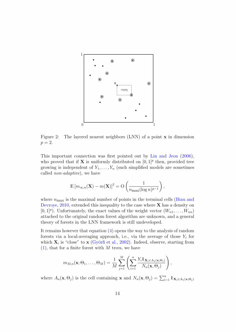
Figure 2: The layered nearest neighbors (LNN) of a point x in dimensionp = 2.

This important connection was first pointed out by Lin and Jeon (2006),who proved that if X is uniformly distributed on [0, 1]p then, provided treegrowing is independent of Y1, . . . , Yn (such simplified models are sometimescalled non-adaptive), we have

E [m∞,n(X)−m(X)]2 = O

(1

nmax(log n)p−1

),

where nmax is the maximal number of points in the terminal cells (Biau andDevroye, 2010, extended this inequality to the case where X has a density on[0, 1]p). Unfortunately, the exact values of the weight vector (Wn1, . . . ,Wnn)attached to the original random forest algorithm are unknown, and a generaltheory of forests in the LNN framework is still undeveloped.

It remains however that equation (4) opens the way to the analysis of randomforests via a local-averaging approach, i.e., via the average of those Yi forwhich Xi is “close” to x (Gyorfi et al., 2002). Indeed, observe, starting from(1), that for a finite forest with M trees, we have

mM,n(x; Θ1, . . . ,ΘM) =1

M

M∑j=1

(n∑i=1

Yi1Xi∈An(x,Θj)

Nn(x,Θj)

),

where An(x,Θj) is the cell containing x and Nn(x,Θj) =∑n

i=1 1Xi∈An(x,Θj)

14

is the number of data points falling in An(x,Θj). Thus,

mM,n(x; Θ1, . . . ,ΘM) =n∑i=1

Wni(x)Yi,

where the weights Wni(x) are defined by

Wni(x) =1

M

M∑j=1

1Xi∈An(x,Θj)

Nn(x,Θj).

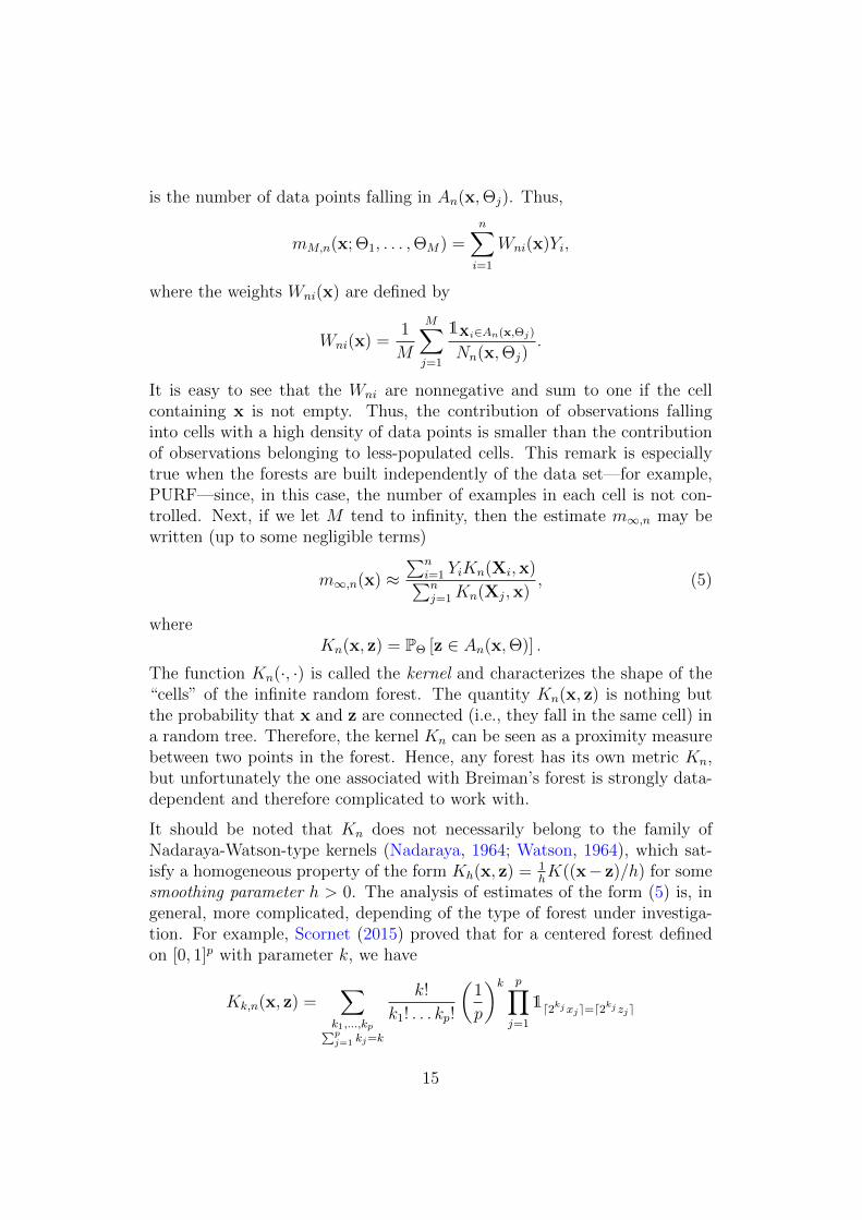
It is easy to see that the Wni are nonnegative and sum to one if the cellcontaining x is not empty. Thus, the contribution of observations fallinginto cells with a high density of data points is smaller than the contributionof observations belonging to less-populated cells. This remark is especiallytrue when the forests are built independently of the data set—for example,PURF—since, in this case, the number of examples in each cell is not con-trolled. Next, if we let M tend to infinity, then the estimate m∞,n may bewritten (up to some negligible terms)

m∞,n(x) ≈∑n

i=1 YiKn(Xi,x)∑nj=1Kn(Xj,x)

, (5)

whereKn(x, z) = PΘ [z ∈ An(x,Θ)] .

The function Kn(·, ·) is called the kernel and characterizes the shape of the“cells” of the infinite random forest. The quantity Kn(x, z) is nothing butthe probability that x and z are connected (i.e., they fall in the same cell) ina random tree. Therefore, the kernel Kn can be seen as a proximity measurebetween two points in the forest. Hence, any forest has its own metric Kn,but unfortunately the one associated with Breiman’s forest is strongly data-dependent and therefore complicated to work with.

It should be noted that Kn does not necessarily belong to the family ofNadaraya-Watson-type kernels (Nadaraya, 1964; Watson, 1964), which sat-isfy a homogeneous property of the form Kh(x, z) = 1

hK((x−z)/h) for some

smoothing parameter h > 0. The analysis of estimates of the form (5) is, ingeneral, more complicated, depending of the type of forest under investiga-tion. For example, Scornet (2015) proved that for a centered forest definedon [0, 1]p with parameter k, we have

Kk,n(x, z) =∑

k1,...,kp∑pj=1 kj=k

k!

k1! . . . kp!

(1

p

)k p∏j=1

1d2kjxje=d2kj zje

15

(d·e is the ceiling function). As an illustration, Figure 3 shows the graphicalrepresentation for k = 1, 2 and 5 of the function fk defined by

fk : [0, 1]× [0, 1] → [0, 1]z = (z1, z2) 7→ Kk,n

((1

2, 1

2), z).

Figure 3: Representations of f1, f2 and f5 in [0, 1]2.

The connection between forests and kernel estimates is mentioned in Breiman(2000a) and developed in detail in Geurts et al. (2006). The most recentadvances in this direction are by Arlot and Genuer (2014), who show that asimplified forest model can be written as a kernel estimate, and provide itsrates of convergence. On the practical side, Davies and Ghahramani (2014)highlight the fact that using Gaussian processes with a specific kernel-basedrandom forest can empirically outperform state-of-the-art Gaussian processmethods. Besides, kernel-based random forests can be used as the inputfor a large variety of existing kernel-type methods such as Kernel PrincipalComponent Analysis and Support Vector Machines.

16

4 Theory for Breiman’s forests

This section deals with Breiman’s (2001) original algorithm. Since the con-struction of Breiman’s forests depends on the whole sample Dn, a mathe-matical analysis of the whole algorithm is difficult. To move forward, theindividual mechanisms at work in the procedure have been investigated sep-arately, namely the resampling step and the splitting scheme.

4.1 The resampling mechanism

The resampling step in Breiman’s (2001) original algorithm is performed bychoosing n times from of n points with replacement to grow the individualtrees. This procedure, which traces back to the work of Efron (1982) (seealso Politis et al., 1999), is called the bootstrap in the statistical literature.The idea of generating many bootstrap samples and averaging predictors iscalled bagging (bootstrap-aggregating). It was suggested by Breiman (1996)as a simple way to improve the performance of weak or unstable learners.Although one of the great advantages of the bootstrap is its simplicity, thetheory turns out to be complex. In effect, the bootstrapped observationshave a distribution that is different from the original one, as the followingexample shows. Assume that X has a density, and note that whenever thedata points are sampled with replacement, then with positive probability,at least one observation from the original sample will be selected more thanonce. Therefore, the resulting Xi of the bootstrapped sample cannot havean absolutely continuous distribution.

The role of the bootstrap in random forests is still poorly understood and, todate, most analyses are doomed to replace the bootstrap by a subsamplingscheme, assuming that each tree is grown with an < n examples randomlychosen without replacement from the initial sample (Mentch and Hooker,2014b; Wager, 2014; Scornet et al., 2015). Most of the time, the subsamplingrate an/n is assumed to tend to zero at some prescribed rate—an assumptionthat excludes de facto the bootstrap regime. In this respect, the analysis ofso-called median random forests by Scornet (2014) provides some insightas to the role and importance of subsampling. The assumption an/n → 0guarantees that every single observation pair (Xi, Yi) is used in them-th tree’sconstruction with a probability that becomes small as n grows. It also forcesthe query point x to be disconnected from (Xi, Yi) in a large proportion oftrees. Indeed, if this were not the case, then the predicted value at x would beoverly influenced by the single pair (Xi, Yi), which would make the ensemble

17

inconsistent. In fact, the estimation error of the median forest estimate issmall as soon as the maximum probability of connection between the querypoint and all observations is small. Thus, the assumption an/n → 0 is buta convenient way to control these probabilities, by ensuring that partitionsare dissimilar enough.

Biau and Devroye (2010) noticed that Breiman’s bagging principle has asimple application in the context of nearest neighbor methods. Recall thatthe 1-nearest neighbor (1-NN) regression estimate sets rn(x) = Y(1)(x), whereY(1)(x) corresponds to the feature vector X(1)(x) whose Euclidean distanceto x is minimal among all X1, . . . ,Xn. (Ties are broken in favor of smallestindices.) It is clearly not, in general, a consistent estimate (Devroye et al.,1996, Chapter 5). However, by bagging, one may turn the 1-NN estimate intoa consistent one, provided that the size of resamples is sufficiently small. Weproceed as follows, via a randomized basic regression estimate ran in which1 ≤ an ≤ n is a parameter. The elementary predictor ran is the 1-NN rulefor a random subsample of size an drawn with (or without) replacement fromDn. We apply bagging, that is, we repeat the random sampling an infinitenumber of times and take the average of the individual outcomes. Thus, thebagged regression estimate r?n is defined by

r?n(x) = E? [ran(x)] ,

where E? denotes expectation with respect to the resampling distribution,conditional on the data set Dn. Biau and Devroye (2010) proved that the es-timate r?n is universally (i.e., without conditions on the distribution of (X, Y ))mean squared consistent, provided an →∞ and an/n→ 0. The proof relieson the observation that r?n is in fact a weighted nearest neighbor estimate(Stone, 1977) with weights

Wni = P(i-th nearest neighbor of x is the 1-NN in a random selection).

The connection between bagging and nearest neighbor estimation is fur-ther explored by Biau et al. (2010), who prove that the bagged estimater?n achieves optimal rate of convergence over Lipschitz smoothness classes,independently from the fact that resampling is done with or without replace-ment.

4.2 Decision splits

The coordinate-split process of the random forest algorithm is not easy tograsp, essentially because it uses both the Xi and Yi variables to make its

18

decision. Building upon the ideas of Buhlmann and Yu (2002), Banerjee andMcKeague (2007) establish a limit law for the split location in the contextof a regression model of the form Y = m(X) + ε, where X is real-valuedand ε an independent Gaussian noise. In essence, their result is as follows.Assume for now that the distribution of (X, Y ) is known, and denote by d?

the (optimal) split that maximizes the theoretical CART-criterion at a givennode. In this framework, the regression estimates restricted to the left andright children of the cell takes the respective forms

β?`,n = E[Y |X ≤ d?] and β?r,n = E[Y |X > d?].

When the distribution of (X, Y ) is unknown, so are β?` , β?r and d?, and these

quantities are estimated by their natural empirical counterparts:

(β`,n, βr,n, dn) ∈ arg minβ`,βr,d

n∑i=1

[Yi − β`1Xi≤d − βr1Xi>d

]2.

Assuming that the model satisfies some regularity assumptions (in particu-lar, X has a density f , and both f and m are continuously differentiable),Banerjee and McKeague (2007) prove that

n1/3(β`,n − β?` , βr,n − β?r , dn − d?)D→ (c1, c2, 1) arg max

tQ(t), (6)

where D denotes convergence in distribution, Q(t) = aW (t)− bt2, and W isa standard two-sided Brownian motion process on the real line. Both a andb are positive constants that depend upon the model parameters and the un-known quantities β?` , β

?r and d?. The limiting distribution in (6) allows one to

construct confidence intervals for the position of CART-splits. Interestingly,Banerjee and McKeague (2007) refer to the study of Qian et al. (2003) onthe effects of phosphorus pollution in the Everglades, which uses split pointsin a novel way. There, the authors identify threshold levels of phosphorusconcentration that are associated with declines in the abundance of certainspecies. In their approach, split points are not just a means to build treesand forests, but can also provide important information on the structure ofthe underlying distribution.

A further analysis of the behavior of forest splits is performed by Ishwaran(2013), who argues that the so-called end-cut preference (ECP) of the CART-splitting procedure (that is, the fact that splits along non-informative vari-ables are likely to be near the edges of the cell—see Breiman et al., 1984)can be seen as a desirable property. Given the randomization mechanism

19

at work in forests, there is indeed a positive probability that none of thepreselected variables at a node are informative. When this happens, and ifthe cut is performed, say, at the center of a side of the cell, then the samplesize of the two resulting cells is drastically reduced by a factor of two—thisis an undesirable property, which may be harmful for the prediction task. Inother words, Ishwaran (2013) stresses that the ECP property ensures that asplit along a noisy variable is performed near the edge, thus maximizing thetree node sample size and making it possible for the tree to recover from thesplit downstream. Ishwaran (2013) claims that this property can be of benefiteven when considering a split on an informative variable, if the correspondingregion of space contains little signal.

There exists a variety of random forest variants based on the CART-criterion.For example, the Extra-Tree algorithm of Geurts et al. (2006) consists in ran-domly selecting a set of split points and then choosing the split that maxi-mizes the CART-criterion. This algorithm has similar accuracy performancewhile being more computationally efficient. In the PERT (Perfect EnsembleRandom Trees) approach of Cutler and Zhao (2001), one builds perfect-fitclassification trees with random split selection. While individual trees clearlyoverfit, the authors claim that the whole procedure is eventually consistentsince all classifiers are believed to be almost uncorrelated. Let us also men-tion that additional randomness can be added in the tree construction byconsidering splits along linear combinations of features. This idea, due toBreiman (2001), has been implemented by Truong (2009) in the packageobliquetree of statistical computing environment R.

4.3 Asymptotic normality and consistency

All in all, little has been proven mathematically for the original procedureof Breiman (2001). Recently, consistency and asymptotic normality of thewhole algorithm were proved under simplifications of the procedure (replac-ing bootstrap by subsampling and simplifying the splitting step). Wager(2014) proves the asymptotic normality of the method and establishes thatthe infinitesimal jackknife consistently estimates the forest variance. A simi-lar result on the asymptotic normality of finite forests, proved by Mentch andHooker (2014b), states that whenever M (the number of trees) is allowed tovary with n, and when an = o(

√n) and limn→∞ n/Mn = 0, then for a fixed

x, √n(mM,n(x; Θ1, . . . ,ΘM)−m∞,n(x))√

a2nζ1,an

D→ N,

20

where N is a standard normal random variable,

ζ1,an = Cov[mn(X1,X2, . . . ,Xan ; Θ),mn(X1,X

′2, . . . ,X

′an ; Θ′)

],

X′i an independent copy of Xi and Θ′ an independent copy of Θ. Notethat in this model, both the sample size and the number of trees grow toinfinity. Recently, Scornet et al. (2015) proved a consistency result in thecontext of additive regression models for the pruned version of Breiman’sforest. Unfortunately, the consistency of the unpruned procedure comes atthe price of a conjecture regarding the behavior of the CART algorithm thatis difficult to verify.

We close this section with a negative but interesting result due to Biau et al.(2008). In this example, the total number k of cuts is fixed and mtry = 1.Furthermore, each tree is built by minimizing the true probability of error ateach node. Consider the joint distribution of (X, Y ) sketched in Figure 4 andlet m(x) = P[Y = 1|X = x]. The variable X has a uniform distribution on[0, 1]2 ∪ [1, 2]2 ∪ [2, 3]2 and Y is a function of X—that is, m(x) ∈ {0, 1} andL∗ = 0—defined as follows. The lower left square [0, 1]× [0, 1] is divided intocountably infinitely many vertical strips in which the strips with m(x) = 0and m(x) = 1 alternate. The upper right square [2, 3] × [2, 3] is dividedsimilarly into horizontal strips. The middle rectangle [1, 2]× [1, 2] is a 2× 2checkerboard. It is easy to see that no matter what the sequence of randomselection of split directions is and no matter for how long each tree is grown,no tree will ever cut the middle rectangle and therefore the probability of errorof the corresponding random forest classifier is at least 1/6. This exampleillustrates that consistency of greedily grown random forests is a delicateissue. Note however that if Breiman’s (2001) original algorithm is used inthis example (i.e., when all cells with more than one data point in them aresplit) then one obtains a consistent classification rule.

5 Variable selection

5.1 Variable importance measures

Random forests can be used to rank the importance of variables in regressionor classification problems via two measures of significance. The first, calledMean Decrease Impurity (MDI), is based on the total decrease in node im-purity from splitting on the variable, averaged over all trees. The second,referred to as Mean Decrease Accuracy (MDA), stems from the idea that if

21

Figure 4: An example of a distribution for which greedy random forestsare inconsistent. The distribution of X is uniform on the union of the threelarge squares. White areas represent the set where m(x) = 0 and grey wherem(x) = 1.

the variable is not important, then rearranging its values should not degradeprediction accuracy.

Set X = (X(1), . . . ,X(p)). For a forest resulting from the aggregation of Mtrees, the MDI of the variable X(j) is defined as

MDI(X(j)) =1

M

M∑`=1

∑t∈T`j?n,t=j

2pn,tLreg,n(j?n,t, z?n,t),

where pn,t(t) is the fraction of observations falling in the node t, {T`}1≤`≤Mthe collection of trees in the forest, and (j?n,t, z

?n,t) the split that maximizes the

empirical criterion (2) in node t. Note that the same formula holds for clas-sification random forests by replacing the criterion Lreg,n by its classificationcounterpart Lclass,n. Thus, the MDI of X(j) computes the weighted decreaseof impurity corresponding to splits along the variable X(j) and averages thisquantity over all trees.

The MDA relies on a different principle and uses the so-called out-of-bagerror estimate. In random forests, there is no need for cross-validation or aseparate test set to get an unbiased estimate of the test error. It is estimated

22

internally, during the run, as follows. Since each tree is constructed using adifferent bootstrap sample from the original data, about one-third of casesare left out of the bootstrap sample and not used in the construction of them-th tree. In this way, for each tree, a test set—disjoint from the trainingset— is obtained, and averaging over all these left-out cases and over all treesis known as the out-of-bag error estimate.

To measure the importance of the j-th feature, we randomly permute thevalues of variable X(j) in the out-of-bag cases and put these cases downthe tree. The MDA of X(j) is obtained by averaging the difference in out-of-bag error estimation before and after the permutation over all trees. Inmathematical terms, consider a variable X(j) and denote by D`,n the out-of-bag test of the `-th tree and Dj`,n the same data set where the values of X(j)

have been randomly permuted. Recall that mn(·,Θ`) stands for the `-th treeestimate. Then, by definition,

MDA(X(j)) =1

M

M∑`=1

[Rn

[mn(·,Θ`),Dj`,n

]−Rn

[mn(·,Θ`),D`,n

]], (7)

where Rn is defined for D = D`,n or D = Dj`,n by

Rn

[mn(·,Θ`),D

]=

1

|D|∑

i:(Xi,Yi)∈D

(Yi −mn(Xi,Θ`))2.

It is easy to see that the population version of MDA(X(j)) takes the form

MDA?(X(j)) = E[Y −mn(X′j,Θ)

]2 − E[Y −mn(X,Θ)]2,

where X′j = (X(1), . . . , X ′(j), . . . , X(p)) and X ′(j) is an independent copy of

X(j). For classification purposes, the MDA still satisfies (7) with Rn(mn(·,Θ),D) the number of points that are correctly classified by mn(·,Θ) in D.

5.2 Theoretical results

In the context of a pair of categorical variables (X, Y ), where X takes finitelymany values in, say, X1 × · · · × Xd, Louppe et al. (2013) consider totallyrandomized and fully developed trees. At each cell, the `-th tree is grown byselecting a variable X(j) uniformly among the features that have not beenused in the parent nodes, and by subsequently dividing the cell into |Xj|children (so the number of children equals the number of modalities of the

23

selected variable). In this framework, it can be shown that the populationversion of MDI(X(j)) for a single tree satisfies

MDI?(X(j)) =

p−1∑k=0

1(kp

)(p− k)

∑B∈Pk(V −j)

I(Xj;Y |B),

where V −j = {1, . . . , j−1, j+ 1, . . . , p}, Pk(V −j) the set of subsets of V −j ofcardinality k, and I(X(j);Y |B) the conditional mutual information of X(j)

and Y given the variables in B. In addition,

p∑j=1

MDI?(X(j)) = I(X(1), . . . , X(p);Y ).

These results show that the information I(X(1), . . . , X(p);Y ) is the sum ofthe importances of each variable, which can itself be made explicit using theinformation values I(X(j);Y |B) between each variable X(j) and the outputY , conditional on variable subsets B of different sizes.

Louppe et al. (2013) define a variable X(j) as irrelevant with respect to B ⊂V = X1 × · · · × Xp whenever I(X(j);Y |B) = 0. Thus, X(j) is irrelevant ifand only if MDI?(X(j)) = 0. It is easy to see that if an additional irrelevantvariable X(p+1) is added to the list of variables, then the variable importanceof any of the X(j) computed with a single tree does not change if the treeis built with the new collection of variables V ∪ {X(p+1)}. In other words,building a tree with an additional irrelevant variable does not change theimportances of the other variables.

The most notable results regarding MDA are due to Ishwaran (2007), whostudies a slight modification of the criterion via feature noising. To add noiseto a variable X(j), one considers a new observation X, take X down the treeand stop when a split is made according to the variable X(j). Then theright or left child node is selected with probability 1/2, and this procedureis repeated for each subsequent node (whether it is performed along thevariable X(j) or not). The importance of variable X(j) is still computed bycomparing the error of the forest with that of the “noisy” forest. Assumingthat the forest is consistent and that the regression function is piecewise

constant, Ishwaran (2007) gives the asymptotic behavior of MDA(X(j)) whenthe sample size tends to infinity. This behavior is intimately related to theset of subtrees (of the initial regression tree) whose roots are split along thecoordinate X(j).

Let us lastly mention the approach of Gregorutti et al. (2013), who computedthe MDA criterion for several distributions of (X, Y ). For example, consider

24

a model of the form

Y = m(X) + ε,

where (X, ε) is a Gaussian random vector, and assume that the correlationmatrix C satisfies C = [Cov(Xj, Xk)]1≤j,k≤p = (1−c)Ip+c11> (the symbol >denotes transposition, 1 = (1, . . . , 1)>, and c is a constant in (0, 1)). Assume,in addition, that Cov(Xj, Y ) = τ0 for all j ∈ {1, . . . , p}. Then, for all j,

MDI?(X(j)) = 2

(τ0

1− c+ pc

)2

.

Thus, in the Gaussian setting, the variable importance decreases as the in-verse of the square of p when the number of correlated variables p increases.

5.3 Related works

The empirical properties of the MDA criterion have been extensively ana-lyzed and compared in the statistical computing literature. Indeed, Archerand Kimes (2008), Strobl et al. (2008), Nicodemus and Malley (2009), Auretand Aldrich (2011), and Tolosi and Lengauer (2011) stress the negative effectof correlated variables on MDA performance. In this respect, Genuer et al.(2010) noticed that MDA is less able to detect the most relevant variableswhen the number of correlated features increases. Similarly, the empiricalstudy of Archer and Kimes (2008) points out that both MDA and MDI be-have poorly when correlation increases—these results have been experimen-tally confirmed by Auret and Aldrich (2011) and Tolosi and Lengauer (2011).An argument of Strobl et al. (2008) to justify the bias of MDA in the presenceof correlated variables is that the algorithm evaluates the marginal impor-tance of the variables instead of taking into account their effect conditionalon each other. A way to circumvent this issue is to combine random forestsand the Recursive Feature Elimination algorithm of Guyon et al. (2002), asin Gregorutti et al. (2013). Detecting relevant features can also be achievedvia hypothesis testing (Mentch and Hooker, 2014b)—a principle that may beused to detect more complex structures of the regression function, like forinstance its additivity (Mentch and Hooker, 2014a).

As for the tree building process, selecting uniformly at each cell a set of fea-tures for splitting is simple and convenient, but such procedures inevitablyselect irrelevant variables. Therefore, several authors have proposed mod-ified versions of the algorithm that incorporate a data-driven weighing of

25

variables. For example, Kyrillidis and Zouzias (2014) study the effectivenessof non-uniform randomized feature selection in decision tree classification,and experimentally show that such an approach may be more effective com-pared to naive uniform feature selection. Enriched random forests, designedby Amaratunga et al. (2008) choose at each node the eligible subsets byweighted random sampling with the weights tilted in favor of informativefeatures. Similarly, the reinforcement learning trees (RLT) of Zhu et al.(2012) build at each node a random forest to determine the variable thatbrings the greatest future improvement in later splits, rather than choosingthe one with largest marginal effect from the immediate split.

Choosing weights can also be done via regularization. Deng and Runger(2012) propose a Regularized Random Forest (RRF), which penalizes select-ing a new feature for splitting when its gain is similar to the features used inprevious splits. Deng and Runger (2013) suggest a Guided RRF (GRRF), inwhich the importance scores from an ordinary random forest are used to guidethe feature selection process in RRF. Lastly, a Garrote-style convex penalty,proposed by Meinshausen (2009), selects functional groups of nodes in trees,yielding to parcimonious estimates. We also mention the work of Konukogluand Ganz (2014) who address the problem of controlling the false positiverate of random forests and present a principled way to determine thresholdsfor the selection of relevant features without any additional computationalload.

6 Extensions

Weighted forests. In Breiman’s (2001) forests, the final prediction is theaverage of the individual tree outcomes. A natural way to improve themethod is to incorporate tree-level weights to emphasize more accurate treesin prediction (Winham et al., 2013). A closely related idea, proposed byBernard et al. (2012), is to guide tree building—via resampling of the train-ing set and other ad hoc randomization procedures—so that each tree willcomplement as much as possible the existing trees in the ensemble. Theresulting Dynamic Random Forest (DRF) shows significant improvement interms of accuracy on 20 real-based data sets compared to the standard, static,algorithm.

Online forests. In its original version, random forests is an offline algo-rithm, which is given the whole data set from the beginning and requiredto output an answer. In contrast, online algorithms do not require that the

26

entire training set is accessible at once. These models are appropriate forstreaming settings, where training data is generated over time and must beincorporated into the model as quickly as possible. Random forests have beenextended to the online framework in several ways (Saffari et al., 2009; De-nil et al., 2013; Lakshminarayanan et al., 2014). In Lakshminarayanan et al.(2014), so-called Mondrian forests are grown in an online fashion and achievecompetitive predictive performance comparable with other online randomforests while being faster. When building online forests, a major difficultyis to decide when the amount of data is sufficient to cut a cell. Exploringthis idea, Yi et al. (2012) propose Information Forests, whose constructionconsists in deferring classification until a measure of classification confidenceis sufficiently high, and in fact break down the data so as to maximize thismeasure. An interesting theory related to these greedy trees can be found inBiau and Devroye (2013).

Survival forests. Survival analysis attempts to deal with incomplete data,and particularly right-censored data in fields such as clinical trials. In thiscontext, parametric approaches such as proportional hazards are commonlyused, but fail to model nonlinear effects. Random forests have been extendedto the survival context by Ishwaran et al. (2008), who prove consistency ofRandom Survival Forests (RSF) algorithm assuming that all variables arefactors. Yang et al. (2010) showed that by incorporating kernel functionsinto RSF, their algorithm KIRSF achieves better results in many situations.Ishwaran et al. (2011) review the use of the minimal depth, which measuresthe predictive quality of variables in survival trees.

Ranking forests. Clemencon et al. (2013) have extended random forests todeal with ranking problems and propose an algorithm called Ranking Forestsbased on the ranking trees of Clemencon and Vayatis (2009). Their approachis based on nonparametric scoring and ROC curve optimization in the senseof the AUC criterion.

Clustering forests. Yan et al. (2013) present a new clustering ensemblemethod called Cluster Forests (CF) in the context of unsupervised classifi-cation. CF randomly probes a high-dimensional data cloud to obtain goodlocal clusterings, then aggregates via spectral clustering to obtain clusterassignments for the whole data set. The search for good local clusteringsis guided by a cluster quality measure, and CF progressively improves eachlocal clustering in a fashion that resembles tree growth in random forests.

Quantile forests. Meinshausen (2006) shows that random forests provideinformation about the full conditional distribution of the response variable,and thus can be used for quantile estimation.

27

Missing data. One of the strengths of random forests is that they canhandle missing data. The procedure, explained in Breiman (2003), takesadvantage of the so-called proximity matrix, which measures the proximitybetween pairs of observations in the forest, to estimate missing values. Thismeasure is the empirical counterpart of the kernels defined in Section 3.2.Data imputation based on random forests has further been explored by Riegeret al. (2010), Crookston and Finley (2008), and extended to unsupervisedclassification by Ishioka (2013).

Forests and machine learning. One-class classification is a binary clas-sification task for which only one class of samples is available for learning.Desir et al. (2013) study the One Class Random Forests algorithm, whichis designed to solve this particular problem. Geremia et al. (2013) have in-troduced a supervised learning algorithm called Spatially Adaptive RandomForests to deal with semantic image segmentation applied to medical imag-ing protocols. Lastly, in the context of multi-label classification, Joly et al.(2014) adapt the idea of random projections applied to the output space toenhance tree-based ensemble methods by improving accuracy while signifi-cantly reducing the computational burden.

References

D. Amaratunga, J. Cabrera, and Y.-S. Lee. Enriched random forests. Bioin-formatics, 24:2010–2014, 2008.

Y. Amit and D. Geman. Shape quantization and recognition with randomizedtrees. Neural Computation, 9:1545–1588, 1997.

K.J. Archer and R.V. Kimes. Empirical characterization of random forestvariable importance measures. Computational Statistics & Data Analysis,52:2249–2260, 2008.

S. Arlot and R. Genuer. Analysis of purely random forests bias.arXiv:1407.3939, 2014.

L. Auret and C. Aldrich. Empirical comparison of tree ensemble variableimportance measures. Chemometrics and Intelligent Laboratory Systems,105:157–170, 2011.

Z.-H. Bai, L. Devroye, H.-K. Hwang, and T.-H. Tsai. Maxima in hypercubes.Random Structures & Algorithms, 27:290–309, 2005.

28

M. Banerjee and I.W. McKeague. Confidence sets for split points in decisiontrees. The Annals of Statistics, 35:543–574, 2007.

O. Barndorff-Nielsen and M. Sobel. On the distribution of the number ofadmissible points in a vector random sample. Theory of Probability andIts Applications, 11:249–269, 1966.

S. Bernard, L. Heutte, and S. Adam. Forest-RK: A new random forest induc-tion method. In D.-S. Huang, D.C. Wunsch II, D.S. Levine, and K.-H. Jo,editors, Advanced Intelligent Computing Theories and Applications. WithAspects of Artificial Intelligence, pages 430–437, Berlin, 2008. Springer.

S. Bernard, S. Adam, and L. Heutte. Dynamic random forests. PatternRecognition Letters, 33:1580–1586, 2012.

G. Biau. Analysis of a random forests model. Journal of Machine LearningResearch, 13:1063–1095, 2012.

G. Biau and L. Devroye. On the layered nearest neighbour estimate, thebagged nearest neighbour estimate and the random forest method in re-gression and classification. Journal of Multivariate Analysis, 101:2499–2518, 2010.

G. Biau and L. Devroye. Cellular tree classifiers. Electronic Journal ofStatistics, 7:1875–1912, 2013.

G. Biau, L. Devroye, and G. Lugosi. Consistency of random forests and otheraveraging classifiers. Journal of Machine Learning Research, 9:2015–2033,2008.

G. Biau, F. Cerou, and A. Guyader. On the rate of convergence of thebagged nearest neighbor estimate. Journal of Machine Learning Research,11:687–712, 2010.

A.-L. Boulesteix, S. Janitza, J. Kruppa, and I.R. Konig. Overview of ran-dom forest methodology and practical guidance with emphasis on compu-tational biology and bioinformatics. Wiley Interdisciplinary Reviews: DataMining and Knowledge Discovery, 2:493–507, 2012.

L. Breiman. Bagging predictors. Machine Learning, 24:123–140, 1996.

L. Breiman. Some infinity theory for predictor ensembles. Technical Report577, University of California, Berkeley, 2000a.

29

L. Breiman. Randomizing outputs to increase prediction accuracy. MachineLearning, 40:229–242, 2000b.

L. Breiman. Random forests. Machine Learning, 45:5–32, 2001.

L. Breiman. Setting up, using, and understanding random forestsV4.0. https://www.stat.berkeley.edu/~breiman/Using_random_

forests_v4.0.pdf, 2003.

L. Breiman. Consistency for a simple model of random forests. TechnicalReport 670, University of California, Berkeley, 2004.

L. Breiman, J.H. Friedman, R.A. Olshen, and C.J. Stone. Classification andRegression Trees. Chapman & Hall/CRC, Boca Raton, 1984.

P. Buhlmann and B. Yu. Analyzing bagging. The Annals of Statistics, 30:927–961, 2002.

S. Clemencon, M. Depecker, and N. Vayatis. Ranking forests. Journal ofMachine Learning Research, 14:39–73, 2013.

S. Clemencon and N. Vayatis. Tree-based ranking methods. IEEE Transac-tions on Information Theory, 55:4316–4336, 2009.

A. Criminisi, J. Shotton, and E. Konukoglu. Decision forests: A unifiedframework for classification, regression, density estimation, manifold learn-ing and semi-supervised learning. Foundations and Trends in ComputerGraphics and Vision, 7:81–227, 2011.

N.L. Crookston and A.O. Finley. yaImpute: An R package for kNN imputa-tion. Journal of Statistical Software, 23:1–16, 2008.

A. Cutler and G. Zhao. PERT – perfect random tree ensembles. ComputingScience and Statistics, 33:490–497, 2001.

D.R. Cutler, T.C. Edwards Jr., K.H. Beard, A. Cutler, K.T. Hess, J. Gibson,and J.J. Lawler. Random forests for classification in ecology. Ecology, 88:2783–2792, 2007.

A. Davies and Z. Ghahramani. The random forest kernel and other kernelsfor big data from random partitions. arXiv:1402.4293, 2014.

H. Deng and G. Runger. Feature selection via regularized trees. In The 2012International Joint Conference on Neural Networks, pages 1–8, 2012.

30

H. Deng and G. Runger. Gene selection with guided regularized randomforest. Pattern Recognition, 46:3483–3489, 2013.

M. Denil, D. Matheson, and N. de Freitas. Consistency of online randomforests. arXiv:1302.4853, 2013.

C. Desir, S. Bernard, C. Petitjean, and L. Heutte. One class random forests.Pattern Recognition, 46:3490–3506, 2013.

L. Devroye, L. Gyorfi, and G. Lugosi. A Probabilistic Theory of PatternRecognition. Springer, New York, 1996.

R. Dıaz-Uriarte and S. Alvarez de Andres. Gene selection and classification ofmicroarray data using random forest. BMC Bioinformatics, 7:1–13, 2006.

T.G. Dietterich. Ensemble methods in machine learning. In Multiple Classi-fier Systems, pages 1–15. Springer, 2000.

B. Efron. The Jackknife, the Bootstrap and Other Resampling Plans, vol-ume 38. CBMS-NSF Regional Conference Series in Applied Mathematics,Philadelphia, 1982.

R. Genuer. Variance reduction in purely random forests. Journal of Non-parametric Statistics, 24:543–562, 2012.

R. Genuer, J.-M. Poggi, and C. Tuleau-Malot. Variable selection using ran-dom forests. Pattern Recognition Letters, 31:2225-2236, 2010.

E. Geremia, B.H. Menze, and N. Ayache. Spatially adaptive random forests.In IEEE International Symposium on Biomedical Imaging: From Nano toMacro, pages 1332–1335, 2013.

P. Geurts, D. Ernst, and L. Wehenkel. Extremely randomized trees. MachineLearning, 63:3–42, 2006.

B. Gregorutti, B. Michel, and P. Saint Pierre. Correlation and variable im-portance in random forests. arXiv:1310.5726, 2013.

I. Guyon, J. Weston, S. Barnhill, and V. Vapnik. Gene selection for cancerclassification using support vector machines. Machine learning, 46:389–422, 2002.

L. Gyorfi, M. Kohler, A. Krzyzak, and H. Walk. A Distribution-Free Theoryof Nonparametric Regression. Springer, New York, 2002.

31

T. Ho. The random subspace method for constructing decision forests. Pat-tern Analysis and Machine Intelligence, 20, 832-844, 1998.

J. Howard and M. Bowles. The two most important algorithms in predictivemodeling today. In Strata Conference: Santa Clara. http://strataconf.com/strata2012/public/schedule/detail/22658, 2012.

T. Ishioka. Imputation of missing values for unsupervised data using theproximity in random forests. In eLmL 2013, The Fifth International Con-ference on Mobile, Hybrid, and On-line Learning, pages 30–36. Interna-tional Academy, Research, and Industry Association, 2013.

H. Ishwaran. Variable importance in binary regression trees and forests.Electronic Journal of Statistics, 1:519–537, 2007.

H. Ishwaran. The effect of splitting on random forests. Machine Learning,99:75–118, 2013.

H. Ishwaran and U.B. Kogalur. Consistency of random survival forests.Statistics & Probability Letters, 80:1056–1064, 2010.

H. Ishwaran, U.B. Kogalur, E.H. Blackstone, and M.S. Lauer. Random sur-vival forests. The Annals of Applied Statistics, 2:841–860, 2008.

H. Ishwaran, U.B. Kogalur, X. Chen, and A.J. Minn. Random survival forestsfor high-dimensional data. Statistical Analysis and Data Mining: The ASAData Science Journal, 4:115–132, 2011.

D. Jeffrey and G. Sanja. Simplified data processing on large clusters. Com-munications of the ACM, 51:107–113, 2008.

A. Joly, P. Geurts, and L. Wehenkel. Random forests with random projec-tions of the output space for high dimensional multi-label classification.In T. Calders, F. Esposito, E. Hullermeier, and R. Meo, editors, MachineLearning and Knowledge Discovery in Databases, pages 607–622, Berlin,2014. Springer.

A. Kleiner, A. Talwalkar, P. Sarkar, and M.I. Jordan. A scalable bootstrapfor massive data. arXiv:1112.5016, 2012.

E. Konukoglu and M. Ganz. Approximate false positive rate control in se-lection frequency for random forest. arXiv:1410.2838, 2014.

32

A. Kyrillidis and A. Zouzias. Non-uniform feature sampling for decision treeensembles. In IEEE International Conference on Acoustics, Speech andSignal Processing, pages 4548–4552, 2014.

B. Lakshminarayanan, D.M. Roy, and Y.W. Teh. Mondrian forests: Efficientonline random forests. In Z. Ghahramani, M. Welling, C. Cortes, N.D.Lawrence, and K.Q. Weinberger, editors, Advances in Neural InformationProcessing Systems, pages 3140–3148, 2014.

P. Latinne, O. Debeir, and C. Decaestecker. Limiting the number of treesin random forests. In J. Kittler and F. Roli, editors, Multiple ClassifierSystems, pages 178–187, Berlin, 2001. Springer.

A. Liaw and M. Wiener. Classification and regression by randomForest. Rnews, 2:18–22, 2002.

Y. Lin and Y. Jeon. Random forests and adaptive nearest neighbors. Journalof the American Statistical Association, 101:578–590, 2006.

G. Louppe, L. Wehenkel, A. Sutera, and P. Geurts. Understanding variableimportances in forests of randomized trees. In C.J.C. Burges, L. Bottou,M. Welling, Z. Ghahramani, and K.Q. Weinberger, editors, Advances inNeural Information Processing Systems, pages 431–439, 2013.

N. Meinshausen. Quantile regression forests. Journal of Machine LearningResearch, 7:983–999, 2006.

N. Meinshausen. Forest Garrote. Electronic Journal of Statistics, 3:1288–1304, 2009.

L. Mentch and G. Hooker. A novel test for additivity in supervised ensemblelearners. arXiv:1406.1845, 2014a.

L. Mentch and G. Hooker. Ensemble trees and CLTs: Statistical inferencefor supervised learning. arXiv:1404.6473, 2014b.

E.A. Nadaraya. On estimating regression. Theory of Probability and ItsApplications, 9:141–142, 1964.

K.K. Nicodemus and J.D. Malley. Predictor correlation impacts machinelearning algorithms: Implications for genomic studies. Bioinformatics, 25:1884–1890, 2009.

D.N. Politis, J.P. Romano, and M. Wolf. Subsampling. Springer, New York,1999.

33

A.M. Prasad, L.R. Iverson, and A. Liaw. Newer classification and regres-sion tree techniques: Bagging and random forests for ecological prediction.Ecosystems, 9:181–199, 2006.

S.S. Qian, R.S. King, and C.J. Richardson. Two statistical methods for thedetection of environmental thresholds. Ecological Modelling, 166:87–97,2003.

A. Rieger, T. Hothorn, and C. Strobl. Random forests with missing values inthe covariates. Technical Report 79, University of Munich, Munich, 2010.

A. Saffari, C. Leistner, J. Santner, M. Godec, and H. Bischof. On-line ran-dom forests. In IEEE 12th International Conference on Computer VisionWorkshops, pages 1393–1400, 2009.

E. Scornet. On the asymptotics of random forests. arXiv:1409.2090, 2014.

E. Scornet. Random forests and kernel methods. arXiv:1502.03836, 2015.

E. Scornet, G. Biau, and J.-P. Vert. Consistency of random forests. TheAnnals of Statistics, in press, 2015.

J. Shotton, A. Fitzgibbon, M. Cook, T. Sharp, M. Finocchio, R. Moore,A. Kipman, and A. Blake. Real-time human pose recognition in partsfrom single depth images. In IEEE Conference on Computer Vision andPattern Recognition, pages 1297–1304, 2011.

C.J. Stone. Consistent nonparametric regression. The Annals of Statistics,5:595–645, 1977.

C.J. Stone. Optimal rates of convergence for nonparametric estimators. TheAnnals of Statistics, 8:1348–1360, 1980.

C.J. Stone. Optimal global rates of convergence for nonparametric regression.The Annals of Statistics, 10:1040–1053, 1982.

C. Strobl, A.-L. Boulesteix, T. Kneib, T. Augustin, and A. Zeileis. Con-ditional variable importance for random forests. BMC Bioinformatics, 9:307, 2008.

V. Svetnik, A. Liaw, C. Tong, J.C. Culberson, R.P. Sheridan, and B.P.Feuston. Random forest: A classification and regression tool for compoundclassification and QSAR modeling. Journal of Chemical Information andComputer Sciences, 43:1947–1958, 2003.

34

L. Tolosi and T. Lengauer. Classification with correlated features: Unre-liability of feature ranking and solutions. Bioinformatics, 27:1986–1994,2011.

A.K.Y. Truong. Fast Growing and Interpretable Oblique Trees via LogisticRegression Models. PhD thesis, University of Oxford, 2009.

H. Varian. Big data: New tricks for econometrics. Journal of EconomicPerspectives, 28:3–28, 2014.

S. Wager. Asymptotic theory for random forests. arXiv:1405.0352, 2014.

S. Wager, T. Hastie, and B. Efron. Standard errors for bagged predictorsand random forests. arXiv:1311.4555, 2013.

G.S. Watson. Smooth regression analysis. Sankhya Series A, pages 359–372,1964.

S.J. Winham, R.R. Freimuth, and J.M. Biernacka. A weighted random forestsapproach to improve predictive performance. Statistical Analysis and DataMining: The ASA Data Science Journal, 6:496–505, 2013.

D. Yan, A. Chen, and M.I. Jordan. Cluster forests. Computational Statistics& Data Analysis, 66:178–192, 2013.

F. Yang, J. Wang, and G. Fan. Kernel induced random survival forests.arXiv:1008.3952, 2010.

Z. Yi, S. Soatto, M. Dewan, and Y. Zhan. Information forests. In InformationTheory and Applications Workshop, pages 143–146, 2012.

R. Zhu, D. Zeng, and M.R. Kosorok. Reinforcement learning trees. TechnicalReport, University of North Carolina, Chapel Hill, 2012.

35