FINAL REPORT

Understanding the Role of Nutrients in Defining

Phytoplankton Responses in the

Trinity-San Jacinto Estuary

By:

Antonietta S. Quigg (Ph.D.)

Principal Investigator

To:

Texas Water Development Board

P.O. Box 13231, Capital Station,

1700 N. Congress Ave., Rm. 462

Austin, TX 78711-3231

Interagency Cooperative Contract

TWDB Contract No. 1104831134

Texas A&M University at Galveston

Department of Marine Biology

200 Seawolf Parkway, Galveston, Texas, 77553

December 2011

2

Table of Contents

Acknowledgements 4

List of Abbreviations and Acronyms 5

1. Abstract 6

2. Introduction 7

2.1 Role of nutrients in Galveston Bay 9

2.2 Towards the development of a nutrient budget 10

2.3 Objectives 11

3. Methods 12

3.1 Freshwater Inflows from the Trinity River 12

3.2 Water quality 12

3.3 Pigments 14

3.4 Phytoplankton Pulse Amplitude Modulated

Fluorometer (PHYTO-PAM) 15

3.5 Plankton collection and identification 16

3.6 Resource Limitation Assays 16

3.7 Statistical analysis 18

4. Results 19

4.1 2011 - Amongst the Warmest and Driest Years on

Record 19

4.2 Freshwater Inflow into Trinity-San Jacinto Estuary

during 2011 20

4.3 Temporal and spatial changes in water quality

at six fixed stations in the Trinity-San

Jacinto Estuary 23

3

4.4 Temporal and spatial distributions of chlorophyll

concentrations measured at six fixed stations in the

Trinity-San Jacinto Estuary 26

4.5 Temporal and spatial changes in TSS measured

at six fixed stations 26

4.6 Temporal and spatial distributions of nutrient

concentrations at six fixed stations 27

4.7 Plankton community composition 30

4.8 Resource Limitation Assays 32

4.9 Pigments 37

4.10 PHYTO-PAM 37

5. Discussion 40

6. Conclusions 43

7. Bibliography 45

4

Acknowledgements

This report is the result of research partially funded by a grant (TWDB Contract No.

1104831134) from the Texas Water Development Board (TWDB) to Antonietta Quigg

(Principal Investigator). The views expressed herein are those of the author and do not

necessarily reflect the views of TWDB. Many people contributed to the successful

completion of this project. From Texas A&M University at Galveston, Tyra Booe, Jamie

Steichen, Rachel Windham, Allison McInnes, Allyson Burgess, Matt Gore and Sam Dorado

participated in all aspects of field work and processing samples in the laboratory; Allison

Parnell performed the statistical analyses. From Texas A&M University, the Geochemical

and Environmental Research Group (GERG) performed the nutrient analysis and from the

TWDB, Carla Guthrie, Robert Burgess and Ruben Solis helped with all aspects of

administering this grant. Also from TWDB, Caimee Schoenbaechler and Carla Guthrie, are

thanked for their contribution in providing comments on the draft report.

5

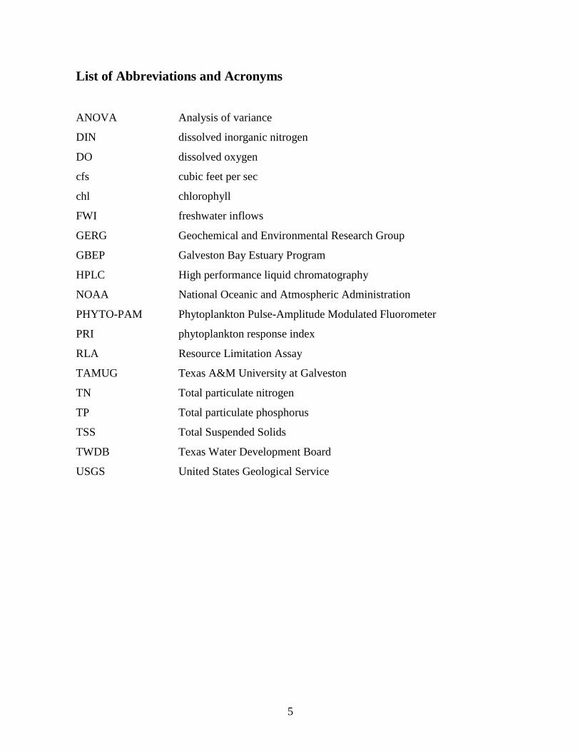
List of Abbreviations and Acronyms

ANOVA Analysis of variance

DIN dissolved inorganic nitrogen

DO dissolved oxygen

cfs cubic feet per sec

chl chlorophyll

FWI freshwater inflows

GERG Geochemical and Environmental Research Group

GBEP Galveston Bay Estuary Program

HPLC High performance liquid chromatography

NOAA National Oceanic and Atmospheric Administration

PHYTO-PAM Phytoplankton Pulse-Amplitude Modulated Fluorometer

PRI phytoplankton response index

RLA Resource Limitation Assay

TAMUG Texas A&M University at Galveston

TN Total particulate nitrogen

TP Total particulate phosphorus

TSS Total Suspended Solids

TWDB Texas Water Development Board

USGS United States Geological Service

6

1. Abstract

The objective of this study was to support continued research aimed at developing an

understanding of nutrient fluxes in the Trinity-San Jacinto Estuary, with the ultimate goal of

determining the nutrient budget for this ecosystem. We examined the effect of the nutrient

loading associated with freshwater inflows (FWI), particularly, those associated with Trinity

River and to a lesser degree, those associated with the San Jacinto River on the phytoplankton

community. Intensive resource limitation assays (RLAs) were performed across six locations

in the Trinity-San Jacinto Estuary during March and July. Given the flows in 2011 were not

very distinctive, we did not compare ―high‖ versus ―low‖ flow but instead compared changes

due to seasons when the strong inflow signal has been depressed. The findings of resource

limitation assays in this study indicate that phytoplankton communities were frequently

limited by ―ALL‖ nutrients, that is, by a combination of nitrate, phosphate and silicate, and

possibly ammonium and frequently co-limited by nitrate and phosphate (+NP treatments) at

all six stations in the Bay. At the three stations located in the southern portion of the Bay,

phytoplankton were also frequently co-limited by nitrate and ammonium (+NA treatments) in

March. The findings are consistent with previous studies which have shown that N limitation

is the dominant process in warmer months and/or at times when there are very little

freshwater flow into the Trinity-San Jacinto Estuary. We found that diatoms plus

dinoflagellates were dominant in March, while cyanobacteria became more important in July.

Partly of this reflects a seasonal transition in the major taxons and partly this reflects

competition for nutrients. Shifts in the dominant phytoplankton groups have consequences to

higher trophic levels including oysters and fish. In terms of developing a nutrient budget for

the Trinity-San Jacinto Estuary, this study was important as it provides important baseline

information on the impact of very low flows in the Trinity-San Jacinto Estuary as 2011 was a

drought year. The reduced freshwater inflows resulted in elevated salinities across the Bay for

much of the year such that by the end of 2011 more than 90% of the Bay had salinities of

greater than 25. The resulting data and conclusions will be essential for developing the next

generation of predictive models relating FWI to bay health.

7

Understanding the Role of Nutrients in Defining

Phytoplankton Responses in the

Trinity-San Jacinto Estuary

2. Introduction

Freshwater inflows (FWI) from rivers, streams, and local runoff maintain the salinity

gradients, nutrient loadings, and sediment inputs that, in combination, produce an

―ecologically sound and healthy estuary.‖ FWI are needed to maintain the unique biological

communities and ecosystems characteristic of a ―healthy‖ estuary (Longley 1994; Nixon

1995). The Texas Water Code (11.147 (a)) beneficial inflows mean ―a salinity, nutrient, and

sediment loading regime adequate to maintain an ecologically sound environment in the

receiving bay and estuary system that is necessary for the maintenance of productivity of

economically important and ecologically characteristic sport or commercial fish and shellfish

species and estuarine life upon which such fish and shellfish are dependent‖. The Galveston

Bay area is likely to see the largest population growth along the Texas coast in the next few

decades (TWDB 2007). We need to understand how the present Trinity-San Jacinto Estuary

(Fig. 1) responds to nutrient and sediment loading from FWI in order to predict the

consequences of human development on the bay ecosystem health and its ability to sustain

local fisheries and to be able to mitigate potential negative impacts of population growth.

In Texas, studies have shown that changes in FWI affect productivity of juvenile brown

shrimp, macrophyte productivity, root:shoot ratios, and species diversity, and benthic

macrofaunal and meiofaunal densities and diversity (Montagna and Kalke 1992; Dunton et al.

1995; Heilman et al. 1999; Riera et al. 2000; Ward et al. 2002; Madrid et al. 2012). Coastal

wetland loss in Louisiana has even been attributed to a reduction in sediment loading as a

result of freshwater diversion (Boesch et al. 1984). Factors equally important, but not as often

addressed, include the magnitude of flushing and nutrient loading, the mode of nutrient

loading, and the ratios of potentially limiting nutrients within the load (Malone et al. 1988;

Chan and Hamilton 2001).

8

Recently conducted resource limitation assays suggest that nitrogen (as nitrate) limits primary

productivity in the Trinity-San Jacinto Estuary (Quigg 2009; Quigg et al. 2010), supporting

earlier studies by Örnólfsdóttir et al. (2004). These recent studies were only performed at two

sites – one in the north and one in the south of the bay (see stars on Fig. 1) - yet they revealed

three new insights:

(i) phytoplankton responded to more strongly to nutrient additions during periods

of low flows than during high flows,

Fig. 1. Texas General Land Office map of the Trinity-San Jacinto estuary. Red

stars on map indicate location of resource limitations assays performed by

Quigg 2009 and Quigg et al., 2010.

9

(ii) there appeared to be differences in response in both scale and species

composition which could be related to the northern versus the southern station

which was associated with the antecedent magnitude of freshwater inflow, and

(iii) phytoplankton are frequently co-limited by several nutrients, typically nitrate

and phosphate.

2.1 Role of Nutrients in Galveston Bay

Nutrients, in the appropriate quantities, contribute positively to water quality and ecosystem

function (Longley 1994; Nixon 1995). However, if present in excessive amounts, nutrients

can lead to the development of harmful algal blooms and other deleterious impacts on

ecosystems health and services (Quigg et al. 2009a,b,c; Quigg 2009, 2010) including but not

limited to algal blooms and fish kills (Thronson and Quigg 2008; McInnes and Quigg 2010).

Excessive nitrogen loading to rivers and estuaries is cited as the principal causal factor of the

rise and spread of eutrophication worldwide (Diaz and Rosenberg 2008). The ―dead zone‖

which appears each summer along the Louisiana coast has long been attributed to loading of

the Mississippi River upstream by the application of fertilizer to crops by farmers in the mid-

west (references in Diaz and Rosenberg 2008).

Guillen (1999) published a report indicating that primary production in Trinity-San Jacinto

Estuary was phosphorus (P) limited while Örnólfsdóttir et al. (2004) reported that it was

nitrogen (N as nitrate) limited. Quigg et al. (2009a) and Quigg (2009) recently reported that

the response of phytoplankton communities to nutrient loading varies both with location and

season in Trinity-San Jacinto Estuary. These authors found evidence of both N and P

limitation, and/or co-limitation by both N and P. While Örnólfsdóttir et al. (2004) also

examined nutrient limitation on spatial (transect from Trinity River to the middle of the

Trinity-San Jacinto Estuary) and temporal (year long study) scales and found that N was the

nutrient limiting growth of phytoplankton; these authors did not consider the San Jacinto

River basin, nor the entrance to Trinity-San Jacinto Estuary at the southern most point which

connects with the Gulf of Mexico (Bolivar Point).

10

Previous studies in Galveston Bay have found phytoplankton production to be dominated by:

cyanobacteria, green algae and diatoms (references in Örnólfsdóttir et al., 2004). While

Örnólfsdóttir et al. (2004), Quigg et al. (2009a) and Quigg (2009) found that diatoms were

the taxa that most often responded to the addition of N sources in their assays, Quigg et al.

(2009a) and Quigg (2009) also observed that when populations were co-limited by N and P,

cryptophytes, haptophytes, prymnesiophytes also responded significantly. The resulting shift

in phytoplankton community composition towards these taxa may not be of concerns because

they are not typically associated with significant harmful algal blooms in the Bay.

Nonetheless, there are a number of noxious species which reside in Texas estuaries,

particularly species of Nitzschia and Pseudonitzschia (Quigg et al. 2009b), which have been

associated with shellfish poisoning from eating mussels and oysters contaminated with

domoic acid.

Buyukates and Roelke (2005) found that plankton assemblages receiving nutrient loads in a

pulsed mode lead to less accumulated phytoplankton biomass and supported greater

secondary productivity, while assemblages receiving a continuous inflow resulted in a

phytoplankton bloom and demise of the zooplankton community. Hence, shifts in

phytoplankton composition may change the nutritional value of phytoplankton communities

to consumers, ranging from zooplankton, oysters and fish at higher trophic levels. This

impact is less well studied but available literature indicates that it may be a cause for concern.

2.2 Towards the development of a nutrient budget

Given the critical role that nutrients play in modulating the base of the food web (primary

producers) in all ecosystems, management efforts directed towards modifying nutrient inputs

(typically reductions in both N and P associated with anthropogenic activities) will have

downstream ecological impacts which are not always clearly understood. For Galveston Bay,

freshwater inflows and waste water treatment facilities are the two most significant point

sources for nitrogen inputs whilst entrainment with Gulf waters is the major loss (Brock

2001). Various efforts over the last three to four decades have focused on developing a

nutrient budget for Galveston Bay (see Galveston Bay Estuary Program website for historical

11

and current studies) to aid in the development of management tools. However, given the

ongoing changes in processes (agriculture, air deposition, reservoir development, urban

development and runoff, and waste water volume and quality) which impact the Bay and

ongoing population growth, the need to develop new nutrient budgets which are responsive to

these changes remains. Further, as flows increase from the San Jacinto River into Galveston

Bay as a result of increased returned flows starting from the Dallas/ Fort Worth Metroplex,

relative to the Trinity River, circulation patterns maybe also altered. All these factors need to

be considered when developing a nutrient budget. Further, bio-geo-chemical processes

talking part in the water column and in the sediment need to be considered. When previous

budget studies have been done (e.g., Brock 2001), the inability to mass balance nitrogen

budgets in the Bay has been associated with a poor understanding of nitrogen processes

occurring both in the water column and in the sediments. Hence, studies such as the current

study, will aid in the development of such budgets, and thereby, tools for managing

ecosystems such as Galveston Bay.

2.3 Objectives

Hence, in this new study we intended to perform intensive resource limitation assays (RLAs)

across six locations in the Trinity-San Jacinto Estuary during a period of typical ―high‖ flows

(March 2011) and then again during a period of typical ―low‖ flows (July 2011), specifically

focusing on the effect of increased nutrient loading impacting phytoplankton community

structure. However, given the actual flows in 2011 were not very distinctive, the results do

not reflect a true response to high versus low flows. Rather, the objective became a

comparison of the phytoplankton responses between seasons when the strong inflow signal

was suppressed. We also investigated the importance of two nitrogen sources – nitrate and

ammonium – on defining both the response and the respondents. This work will be

conducted concurrently with other funded programs examining freshwater inflows in

Galveston Bay, providing important insights specifically towards understanding the role of

nutrients in defining phytoplankton responses in the Trinity-San Jacinto Estuary.

12

3. Methods

3.1 Freshwater Inflows from the Trinity River

Real-time flow data from a USGS monitoring station (Trinity River at Romayor; USGS

gauge 08066500) was used to determine the freshwater inflow volume into the Trinity-San

Jacinto Estuary from January to December 2011. By summing the daily flows provided on

the USGS web site, we determined the total monthly and annual flow (cfs) from the Trinity

River respectively. In order to report flows inflows and water volumes in acre-feet, we used

the conversation factor 1.983471 (Qingguang Lu; TWDB hydrologist), that is, 1 cubic foot

per sec (cfs) for 24 hours = 1.983471 acre-feet. We summed daily flows in acre-feet to

determine the total monthly and annual flow from the Trinity River respectively.

3.2 Water Quality

Immediately prior to starting the resource limitation assays at six fixed stations (Fig. 2; Table

1) in March (15 and 16 2011) and in July (11 and 12 2011), water profiles were measured

with a calibrated Hydrolab: temperature, salinity, dissolved oxygen and pH were recorded at

1m intervals from the surface to the bottom of the water column. Salinity (throughout the

report) will be reported using the Practical Salinity Scale according to UNESCO (1981). The

Practical Salinity Scale defines salinity as a pure ratio, and has no dimensions or units.

Further, it will not have any numerical symbol to indicate parts per thousand. Salinity will

thus be reported as a number with no symbol or indicator of proportion after it. In particular,

it is not correct to add the letters PSU, implying Practical Salinity Units, after the number. A

single water column profile was taken at each station prior to collecting water for water

quality analysis (see below) and prior to starting the resource limitation assays (see below

also).

13

Table 1: Latitude and longitude of fixed sampling stations in Trinity-San Jacinto Estuary.

Station Latitude Longitude Site description

1 29°71.15' 94°74.58' Upper Trinity River Basin

2 29°61.60' 94°82.90' Lower Trinity River Basin

3 29°51.21' 94°85.68' Middle Bay

4 29°40.36' 94°86.81' Lower Bay

5 29°35.76' 94°75.81' Bolivar Pass

6 29°61.08' 94°92.86' San Jacinto River Basin

Additional water was collected from surface waters to measure (i) chlorophyll a (chl a), (ii)

dissolved (nitrate, nitrite, ammonia, urea, silicate and phosphate) and total (nitrogen (TN) and

Fig. 2 Map showing location

of six fixed sampling stations

in the Trinity-San Jacinto

Estuary.

14

phosphorus (TP)) nutrients, (iii) total suspended solids (TSS), (iv) pigments and (v) to

examine the phytoplankton community using microscopy.

Water from each of these stations was filtered (GF/F; Whatman) onto filters under low

vacuum pressure (< 130 kPa). Filters were folded and frozen at -20°C for later chl a analysis.

Calibration and measurement techniques were performed according to Arar and Collins

(1997) with some modifications described in Quigg et al. (2007, 2009).

For nutrient (dissolved and total) analysis, water samples from each station were filtered

(GF/F; Whatman) onto a filter under low vacuum (< 130 kPa) pressure. The filtrate was

stored in an acid cleaned HDPE rectangular bottle (125 mL; Nalgene) which was triple rinsed

with extra filtrate before keeping the final sample for analysis. Total nutrients were measured

on unfiltered samples. Samples for nutrient analysis were frozen immediately until analysis

by Geochemical and Environmental Research Group (GERG) at TAMU (College Station).

The ratio of inorganic nitrogen (DIN) to phosphate (P = PO4-P) nutrients was calculated after

summing the nitrogen inputs (DIN = NO3-N + NO2-N + NH4-N).

For measurement of total suspended solids, filters were pre-combusted (500ºC for 5 hrs) and

pre-weighed. After filtration of a known volume of water, filters were dried in an oven at 60

ºC for no less than 48 hrs and then reweighed.

3.3 Pigment Analysis

The relative abundance of microalgal groups in mixed species assemblages can be assessed

using the diversity and phylogenetic association of specific photosynthetic accessory

pigments (chlorophylls and carotenoids) (Millie et al. 1993, Jeffrey et al. 1997). Mackey et

al. (1996) developed an analysis algorithm (CHEMTAX) for calculating algal class

abundances based on biomarker photopigments. High performance liquid chromatography

(HPLC) was performed using standard protocols (Millie et al. 1993; Jeffrey et al. 1997).

Essentially, aliquots (0.3 to 1.0 L) of water collected from the six fixed stations (Fig. 2) were

filtered under a gentle vacuum (<50 kPa) onto 4.7 cm diameter filters (Whatman GF/F),

15

immediately frozen, and stored at -80° C. Frozen filters were then cut into strips and placed

into a freeze dryer for 12-24 hours. Then filters were then placed in 100% acetone (3 mL),

and extracted at -20° C for 12 - 20 h. Filtered extracts (200 µL) were injected into a

Shimadzu HPLC equipped with a single monomeric (0.46 x 10 cm, 3 µm) and two polymeric

(0.46 x 25 cm, 5 µm) reverse-phase C18 columns in series according to their properties (Van

Heukelem et al. 1994; Jeffrey et al. 1997). A nonlinear binary gradient, adapted from Van

Heukelem et al. (1994), was used for pigment separations. Solvent A consists of 80%

methanol:20% ammonium acetate (0.5 M adjusted to pH 7.2) and solvent B is 80% methanol:

20% acetone. Absorption spectra and chromatograms (440 nm) were acquired using a

Shimadzu SPD-M10av photodiode array detector. Pigment peaks were identified by

comparison of retention times and absorption spectra with pure crystalline standards,

including chlorophylls a, b, -carotene (Sigma Chemical Company), fucoxanthin, and

zeaxanthin (Hoffman-LaRoche and Company). Other pigments were identified by

comparison to extracts from phytoplankton cultures and quantified using the appropriate

extinction coefficients (Jeffrey et al. 1997).

3.4 Phytoplankton Pulse - Amplitude Modulated Fluorometer

(PHYTO-PAM)

The pulse-amplitude-modulation (PAM) measuring principle is based on selective

amplification of a fluorescence signal which is measured in the presence of intense, but very

short (μsec) pulses of actinic light. In the PHYTO-PAM, light pulses are generated by an

array of light-emitting diodes featuring 4 different wavelengths: blue (470 nm), green (520

nm), light red (645 nm) and dark red (665 nm). This feature is very useful for distinguishing

algae with different types of photosynthetic accessory pigments (Jakob et al. 2005). Green

algae (Chlorophytes and Prasinophytes) can be distinguished from Diatoms plus

Dinoflagellates and Cyanophyta. The advantage of the PHYTO-PAM technique is that it can

be done in minutes (compared with hrs-to-days for HPLC). The PHYTO-PAM approach

promises to be particularly suited to monitoring programs as it is also very sensitive (to 0.1

µg chlorophyll L-1

) (Nicklisch and Köhler 2001) and allows for statistically robust

16

experimental design given many samples can be examined within a short period of time. In

this study, the PHYTO-PAM was used to obtain a rapid assessment of the dominant

phytoplankton community in the RLAs. Previous studies have shown this is useful for

determining the major microalgal groups (Quigg et al. 2009b,c).

3.5 Plankton collection and identification

Phytoplankton were collected by towing a 67 m net in the water for no less than five

minutes. This was used to concentrate plankton into a 50 mL sample which was preserved in

an acid cleaned HDPE rectangular bottle (125 mL; Nalgene) using Gluteraldehyde (final 5%).

Samples were examined microscopically for general species identification with the assistance

of Tomas (1997). Digital photographs of representatives of each species were recorded along

with the magnification, sizes and any other distinguishing detail.

3.6 Resource Limitation Assays (RLAs)

Resource limitation assays (RLA) were undertaken to identify which resource (nutrient(s)

and/or light) limited phytoplankton growth at six sampling sites in Trinity-San Jacinto

Estuary (Fig. 2; Table 1). Sampling occurred from March 15 to 16 2011 and from July 11 to

12 2011. In the 30 day period preceding these sampling campaigns, a total of 53,240 cfs

(105,600 acre-feet) and 54,540 cfs (108,179 acre-feet) were discharged respectively. That is,

a similar amounts of FWI’s preceding the March and July sampling events. Bioassays were

carried out essentially as described by Fisher et al. (1999) with modifications as described in

Quigg et al. (2009c, 2010). Specifically, in this particular study, surface (0 - 0.5 m) water was

collected from the six stations for ten treatments performed in triplicate (total 180 cubitainers)

and an “initial control” (total 6 cubitainers). The initial phytoplankton biomass (as chl a) and

community composition (HPLC, PHYTO-PAM) were measured in the initial control.

The following treatments were performed in March and July:

(i) C control (no additions, no modifications),

(ii) N plus nitrogen (N as nitrate, 30 mol L-1

NO3-),

17

(iii) A plus nitrogen (N as ammonium, 30 mol L-1

NH4+),

(iv) P plus phosphorus (as phosphate, 2 mol L-1

PO43-

),

(v) NP plus nitrate and phosphate,

(vi) NA plus nitrate and ammonium,

(vii) Si plus silicate (30 mol L-1

SiO3)

(viii) ALL plus nitrate, ammonium, phosphate and silicate

(ix) G grazing (filter water thru a 118 m mesh),

(x) Sh shade (block light penetration by 50%).

Fig. 3 Experimental set up - each sample was incubated at ambient water temperatures, turbulence

and under 50% ambient sunlight in an outdoor facility at TAMUG. At the end of the experiment the

180 cubitainers are retrieved and processed in the laboratory.

18

The nutrient concentrations above are the final concentrations of each nutrient in each

treatment; the experiments were designed to provide excess nutrients. For the grazing

treatment, no nutrients were added (as done for the control) but the water was pre-filtered

with a 118 m filter before filling each cubitainer. Treatments were incubated at ambient

water temperatures, turbulence and under 50% ambient sunlight in an outdoor facility (Fig.

3). Free floating corrals were designed to fit 30 cubitainers in each of six quadrants.

Cubitainers were randomly loaded into these units within hours of sample collection.

Treatments were then left for a week before being sub-sampled for changes in phytoplankton

biomass (as chl a) and community composition (HPLC, PHYTO-PAM). Cubitainers were

collected and processed as quickly as possible in the laboratory; a low light (shaded)

environment.

The response potential of phytoplankton in each treatment was quantified according to the

phytoplankton response index (PRI) of Fisher et al. (1999). The PRI was calculated by

determining the phytoplankton growth response as the ratio of the maximum biomass relative

to the initial biomass. Given that the ―initial‖ biomass was measured at the start of the

experiment and the ―maximum‖ biomass was that measured at the end of the experiment (one

week later), the PRI reflects the change in biomass over the duration of the RLA.

3.7 Statistical analysis

SPSS statistical software was used to perform a Kruskall-Wallis Test to determine significant

differences between water quality parameters (temperature, salinity, LDO, and pH), water

column nutrients (nitrate, nitrite, nitrate + nitrite, ammonium, urea, silicate, phosphate) and

elemental ratios across all stations between March and July. A Mann Whitney U Test was

used to determine differences in salinity between station 1 and station 6 in March. Analysis

of variance (ANOVA) was used to determine significant differences in TN and TP

concentrations across all stations between March and July. A Kruskall-Wallis Test was used

to determine significant differences between PRIs across all stations and treatments for each

month. A Mann Whitney U Test was used to determine differences in PRIs within all

treatments and across all stations for March and July.

19

4. Results

When values presented in the report are mean values we have included standard deviations.

However, in most cases including the USGS data, the water quality data collected with the

hydrolab and the plankton identification work, replicate measurements are not available.

4.1 2011 – Amongst the Warmest and Driest Years on Record

2011 was amongst the warmest and driest years on record since records started in 1871 in

Texas (www.nws.noaa.gov). The City of Houston experienced the warmest year on record,

matching the previous record set in 1962. The City of Galveston recorded its second warmest

year on record, with 2006 established as the warmest year since record keeping started. For

comparison, the five warmest years on record for cites adjacent to the Trinity-San Jacinto

Estuary are listed in Table 2 (data from www.nws.noaa.gov).

Table 2. Five warmest years (listed in order of highest to lowest) on record for cites adjacent to

the Trinity-San Jacinto Estuary.

City of Houston Houston Hobby City of Galveston

1 71.9°F 1962 72.4°F 2011 72.6°F 2006

2 71.9°F 2011 72.3°F 1998 72.5°F 2011

3 71.7°F 1933 71.4°F 2006 72.3°F 2005

4 71.5°F 1965 71.3°F 2008 72.3°F 1994

5 71.5°F 1927 71.1°F 2009 72.3°F 1999

In terms of rainfall, 2011 was one of the top five driest years on record for the Galveston Bay

watershed (www.nws.noaa.gov). The City of Houston received ~25 inches of rain in 2011

making this the third driest year on record (Table 3) while the City of Galveston received ~

23 inches of rain in 2011 (Table 3). This is at about 30 to 50 percent of the expected normal

rainfall for the City of Houston, Houston Hobby and City of Galveston which typically

receive 49.77, 54.65 and 50.76 inches of rain respectively (www.nws.noaa.gov).

20

Table 3. Rainfall (inches) recorded for five driest years (listed in order of lowest to highest) on record

for cites adjacent to the Trinity-San Jacinto Estuary.

City of Houston Houston Hobby City of Galveston

1 17.66 1917 25.41 2011 21.40 1948

2 22.93 1988 26.65 1988 21.43 1917

3 24.57 2011 28.32 1956 21.84 1956

4 27.09 1901 28.76 1954 22.29 1954

5 27.23 1951 31.11 1931 22.95 2011

4.2 Freshwater Inflow into Trinity-San Jacinto Estuary during 2011

Real-time freshwater inflow measured as daily discharge (www.waterdata.usgs.gov) in cubic

feet per second (cfs) to Trinity-San Jacinto Estuary from January 01 to December 31 2011

was downloaded from the USGS monitoring gauge located on the Trinity River at Romayor

(08066500), and for comparison, from January 01 to December 31 2010. The corresponding

gage height (feet) was also downloaded for these two time periods.

Consistent with the year having little rainfall, there was little freshwater inflow into the

Trinity-San Jacinto Estuary from the Trinity River (Fig. 4). The annual (total) discharge in

2011 was 656,466 cfs (~1.3 million acre-feet), about 20% of the total discharge (2,973,821

cfs; ~5.9 million acre-feet) recorded in 2010 (Fig. 6). In addition, river levels fell

significantly (Fig. 5) compared to the previous year (Fig. 7). Typically, most of the freshwater

inflows into the Trinity-San Jacinto Estuary occur in the fall but significant freshwater inflow

events (>10,000 cubic feet per sec) or freshets also occur during the spring. This was

observed in 2010 but not 2011 (Figs. 6 and 4 respectively). In fact in 2011 there were no

freshets >10,000 cfs. This is consistent with suppressed flows due to drought conditions in

2011.

Based on previous yearly flow events, we performed the RLAs in March and July. However,

given the unusual conditions in 2011 we were not able to compare responses to ―high‖ and

―low‖ flows, as the flows were similar prior to each sampling event (see section 3.6 above)

but instead compared the seasonal signal (March versus July) with the inflows ―turned off‖.

21

Fig. 4 Daily discharge (cfs) from the Trinity River in 2011 (www.waterdata.usgs.gov).

Fig. 5 Daily gage height (cfs) on the Trinity River in 2011 (www.waterdata.usgs.gov).

22

Fig. 6 Daily discharge (cfs) from the Trinity River in 2010 and 2011 (www.waterdata.usgs.gov).

Fig. 7 Daily gage height (cfs) on the Trinity River in 2010 and 2011 (www.waterdata.usgs.gov).

23

4.3 Temporal and spatial changes in water quality measured at the

six fixed stations

Water quality was measured at each station immediately prior to commencing the RLAs.

During both months, the water column was well mixed as can be seen in Tables 5 and 6

below. We found water temperatures were significantly lower (p < 0.001) in March than

July, on average 17.95ºC ±0.32ºC and 30.51ºC ±0.43ºC respectively. These temperature

ranges are typical for this ecosystem (Davis et al. 2007; Quigg et al. 2007; 2009c).

Salinities on average were significantly different (p = 0.002) between March (22.3 ±3.7) and

July (25.9 ±2.8). There was nonetheless a gradient of increasing salinities in March from

station 1 to 5 (Table 5) which corresponds to stations located in the upper Trinity River Basin

(station 1) adjacent to the mouth of the Trinity River to station 5, located at Bolivar Pass and

the Gulf of Mexico (Fig. 2). Salinities increased from 15.1 to 27.2 (Table 5). The salinity in

the San-Jacinto River Basin (station 6, 21.9) was significantly higher (p = 0.034) than that in

the upper Trinity River Basin (station 1, 15.1) consistent with typically greater freshwater

inputs from the latter river relative to the former (Table 5). Whilst there was also a gradient in

July, this was less steep, with salinities varying from 22 to 30 from stations 1 to 5 and the

salinities in both river basins being similar (~23-24) (Table 6).

Dissolved oxygen (DO) concentrations on average were significantly different (p < 0.0001)

between March (8.06 ±0.06) and July (5.68 ±0.79) (Table 5 and 6). Given that the %DO was

less than 100 for both months, it is unlikely that there were blooms present at any of the six

stations prior to commencing the RLAs.

We found a significant difference (p < 0.0001) in water column pH between March and July,

on average 7.96 ±0.02 and 8.07 ±0.05 respectively, although this change was small.

24

.

Table 5 Water quality parameters measured at the fixed stations immediately prior to performing the

RLAs in March 2011.

Depth Temperature Salinity

Conductivity

(SpC) LDO LDO% pH

m º C PSU mS cm-1

mg/L %

1 0 17.69 15.14 24.94 8.30 95.3 7.93

1 17.7 15.14 24.94 8.22 94.4 7.97

2 17.69 15.14 24.95 8.14 93.4 7.98

2 0 17.6 19.91 31.96 8.25 97.3 7.94

1 17.6 19.91 31.97 8.15 96.2 7.96

2 17.6 19.91 31.96 8.13 95.9 7.97

2.5 17.59 19.90 31.95 8.06 95.1 7.97

3 0 18.09 23.34 36.85 7.93 96.3 7.89

1 18.09 23.35 36.84 7.87 95.7 7.90

2 18.08 23.35 36.86 7.84 95.4 7.90

3 18.08 23.37 36.91 7.81 95.1 7.90

4 0 18.62 23.21 36.70 8.53 104.8 8.06

1 18.63 23.21 36.69 8.81 104.6 8.06

2 18.63 23.21 36.67 8.49 104.2 8.06

5 0 18.04 27.19 42.26 7.94 98.8 8.05

1 18.04 27.19 42.30 7.90 98.3 8.05

2 17.97 27.27 42.38 7.87 97.8 8.05

3 17.96 27.28 42.42 7.84 97.5 8.05

4 17.96 27.29 42.40 7.82 97.2 8.05

6 0 17.76 21.91 34.84 8.04 95.6 7.79

1 17.75 21.91 34.83 7.75 93.0 7.80

2 17.69 21.93 34.85 7.63 91.3 7.81

Station

25

Table 6 Water quality parameters measured at the fixed stations immediately prior to performing the

RLAs in July 2011.

Depth Temperature Salinity

Conductivity

(SpC) LDO LDO% pH

m º C PSU mS cm-1

mg/L %

1 0 30.49 22.10 35.10 6.04 90.9 8.02

1 30.49 22.10 35.12 5.98 89.9 8.02

2 30.49 22.10 35.12 5.87 88.3 8.02

2 0 30.75 24.37 38.33 6.52 99.9 8.21

1 30.53 24.37 38.31 6.53 99.2 8.21

2 30.4 24.36 38.30 6.38 95.3 8.18

3 30.36 24.34 38.28 5.80 86.4 8.16

3 0 30.43 25.78 40.29 5.44 82.6 8.08

1 30.38 25.77 40.29 5.32 81.5 8.07

2 30.36 25.77 40.29 5.23 80.1 8.06

3 30.36 25.76 40.28 5.18 79.5 8.07

4 0 31.44 27.01 42.03 5.57 87.4 8.13

1 31.06 27.00 42.00 5.33 83.3 8.11

2 31.07 27.00 42.00 5.34 83.4 8.11

5 0 29.86 30.90 47.36 4.50 70.3 7.95

1 29.87 30.91 47.38 4.48 70.1 7.95

2 29.91 31.14 47.61 4.45 69.9 7.96

3 29.93 31.33 47.97 4.54 71.4 7.98

6 0 31.43 24.34 38.28 7.09 109.9 8.08

1 30.54 24.46 38.46 7.10 107.9 8.07

2 30.51 25.37 39.73 6.28 95.7 8.07

3 30.51 25.48 39.87 5.99 90.9 8.04

Station

26

4.4 Temporal and spatial changes in Chl a concentration measured

at the six fixed stations

Chlorophyll (chl; ug/L) a is often used as a proxy for phytoplankton biomass and so it is

likely to vary on both temporal and spatial scales across the Trinity-San Jacinto Estuary. In

general phytoplankton biomass was lower in March than in July throughout the bay (Table 7).

While in March there was about half as much chl a at Station 6 (4.66 ug/L) as in Station 1

(8.73 ug/L), in July, there were similar amounts of chl a at both these stations (Table 7).

Stations 1 and 6 are those most likely to impacted by the Trinity and San Jacinto River

inflows respectively.

4.5 Temporal and spatial changes in TSS measured at the six fixed

stations

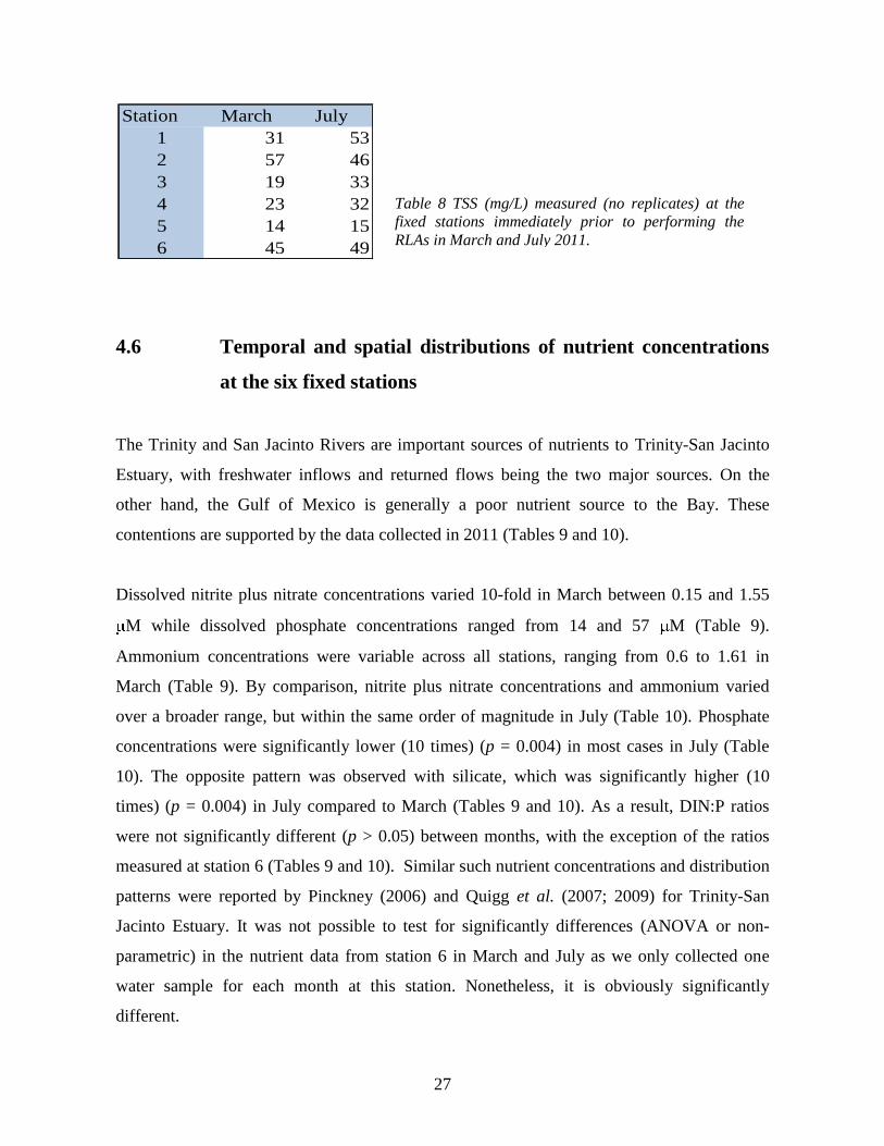
Total sediment loading in the Trinity-San Jacinto Estuary was estimated from measurements

of TSS concentrations (Table 8), that is, the TSS values were used as indicators of sediment

concentrations in the water column. These are only proxies of loading as TSS values are also

influenced by other processes which include but are not limited to wind induced mixing and

resuspension events. The TSS values in Table 8 are typical of low flow periods in the Trinity-

San Jacinto Estuary (see Quigg 2010). Given the unusual flow conditions in 2011, this is not

unexpected.

Station March July

1 8.73 16.83

2 16.40 13.85

3 3.79 15.56

4 5.25 11.78

5 11.69 8.36

6 4.66 14.16

Table 7 Chl a (ug/L) measured (no replicates) at the

fixed stations immediately prior to performing the

RLAs in March and July 2011.

27

4.6 Temporal and spatial distributions of nutrient concentrations

at the six fixed stations

The Trinity and San Jacinto Rivers are important sources of nutrients to Trinity-San Jacinto

Estuary, with freshwater inflows and returned flows being the two major sources. On the

other hand, the Gulf of Mexico is generally a poor nutrient source to the Bay. These

contentions are supported by the data collected in 2011 (Tables 9 and 10).

Dissolved nitrite plus nitrate concentrations varied 10-fold in March between 0.15 and 1.55

M while dissolved phosphate concentrations ranged from 14 and 57 M (Table 9).

Ammonium concentrations were variable across all stations, ranging from 0.6 to 1.61 in

March (Table 9). By comparison, nitrite plus nitrate concentrations and ammonium varied

over a broader range, but within the same order of magnitude in July (Table 10). Phosphate

concentrations were significantly lower (10 times) (p = 0.004) in most cases in July (Table

10). The opposite pattern was observed with silicate, which was significantly higher (10

times) (p = 0.004) in July compared to March (Tables 9 and 10). As a result, DIN:P ratios

were not significantly different (p > 0.05) between months, with the exception of the ratios

measured at station 6 (Tables 9 and 10). Similar such nutrient concentrations and distribution

patterns were reported by Pinckney (2006) and Quigg et al. (2007; 2009) for Trinity-San

Jacinto Estuary. It was not possible to test for significantly differences (ANOVA or non-

parametric) in the nutrient data from station 6 in March and July as we only collected one

water sample for each month at this station. Nonetheless, it is obviously significantly

different.

Station March July

1 31 53

2 57 46

3 19 33

4 23 32

5 14 15

6 45 49

Table 8 TSS (mg/L) measured (no replicates) at the

fixed stations immediately prior to performing the

RLAs in March and July 2011.

28

Table 9 Nutrient parameters measured at the fixed stations immediately prior to performing the RLAs

in March 2011. Nitrate (NO3-), HPO4

-(phosphate), silicate (HSiO3

-), ammonium (NH4

+), nitrite (NO2

-),

urea, total particulate nitrogen (TN) and total particulate phosphate (TP) were measured. The

following were calculated: Nitrate plus nitrite (NO3- + NO2

-), dissolved inorganic nitrogen (DIN) and

DIN:P.

Table 10 Nutrient parameters measured at the fixed stations immediately prior to performing the

RLAs in March 2011. Nitrate (NO3-), HPO4

-(phosphate), silicate (HSiO3

-), ammonium (NH4

+), nitrite

(NO2-), urea, total particulate nitrogen (TN) and total particulate phosphate (TP) were measured. The

following were calculated: Nitrate plus nitrite (NO3- + NO2

-), dissolved inorganic nitrogen (DIN) and

DIN:P.

The Trinity River is frequently a greater source of dissolved nutrients to Trinity-San Jacinto

Estuary than the San Jacinto River. Using the nutrient concentrations from Station 1 and 6

respectively (Fig. 2), we can get an image of the nutrient inputs by these two rivers to the

Bay. In 2011, we found that the San Jacinto River supplied higher concentrations of nitrite

NO3-

HPO4-

HSiO3-

NH4+

NO2- Urea

NO3- +

NO2- DIN DIN:P Total N Total P TN:TP

uM uM uM uM uM uM uM uM uM uM

1 0.79 31.333 0.34 0.83 11.1 0.31 0.154 0.04 0.5 0.54 0.6506 44.79

2 0.51 57.333 0.4 0.6 6.46 1.14 0.138 0.44 0.54 0.98 1.6333 41.78

3 1.02 19.333 4.69 1.32 10.55 5.66 0.653 0.64 5.34 5.98 4.5303 56.28

4 1.22 22.667 0.05 0.55 2.61 0.26 0.107 0.11 0.16 0.27 0.4909 33.66

5 0.98 14 0.05 0.66 4.07 1.07 0.224 0.63 0.27 0.9 1.3636 27.05

6 0.56 44.667 15.6 1.61 13.08 6.71 1.557 0.79 17.16 17.95 11.149 70.26

Station

NO3-

HPO4-

HSiO3-

NH4+

NO2- Urea

NO3- +

NO2- DIN DIN:P Total N Total P TN:TP

uM uM uM uM uM uM uM uM uM uM

1 0.05 3.02 75.95 0.22 0.07 0.31 0.12 0.43 0.14 66.03 3.80 17.38

2 0.06 1.44 25.77 0.41 0.10 0.19 0.16 0.35 0.24 56.03 4.14 13.53

3 0.61 1.89 29.86 1.05 3.83 0.32 4.44 4.76 2.52 53.83 2.07 26.00

4 0.06 0.75 42.67 2.41 0.04 0.02 0.10 0.12 0.15 37.78 1.28 29.52

5 0.96 0.71 30.33 0.60 1.69 0.23 2.66 2.89 4.06 27.50 0.45 61.11

6 0.07 1.66 22.57 0.62 0.08 0.09 0.14 0.23 0.14 63.34 2.71 23.37

Station

29

plus nitrate, urea, ammonium, silicate and phosphate than the Trinity River in March (Table

9). In July, the two rivers supplied similar concentrations of nitrite plus nitrate but not the

other nutrients (Table 10). The Trinity River supplied higher concentrations of phosphate,

silicate and urea but not ammonium in July (Table 10). A Kruskall Wallis test did not reveal

any significant difference between nutrient concentrations at station 1 and 6 for March or

July.

In general, a DIN: P ratio in the range of 7:1 to 12:1 by mass is associated with plant growth

being limited by neither phosphorus nor nitrogen. If the DIN:P ratio is greater than 12:1,

phosphorus tends to be limiting, and if the DIN:P ratio is less than 7:1, nitrogen tends to be

limiting (Wetzel 2001; Howarth and Marino 2006). During March and July, DIN:P ratios

were less than 7.1 at all stations except one (station 6 in March) indicating the potential for N

limitation of phytoplankton growth. This is typically observed at these stations in the

summer in the Trinity-San Jacinto Estuary but less so in the spring (Quigg et al. 2007; 2009).

While dissolved nutrient concentrations are those most bioavailable to phytoplankton, total

particulate nutrient concentrations are nonetheless an important component of the water

quality characteristics of any system and may be available to some fraction of the community.

TN and TP concentrations measured at the six fixed stations are summarized in Tables 9 and

10. Consistent with our understanding that different processes regulate the different nutrient

fractions, patterns observed for total particulate nutrients were not identical to those observed

for dissolved nutrients.

The total particulate nitrogen (TN) concentrations were significantly lower (p < 0.0001) in

March (Table 9) relative to July (Table10). This pattern was also observed for total

particulate phosphorus (TP) concentrations although not significant (p > 0.05) (Tables 9 and

10). TN:TP ratios suggest a strong potential for P-limitation of phytoplankton predominantly

in the spring (ratios > 27 in March) but less so in the summer (ratios > 13). Patterns for TN

and TP were not the same as observed previously. Whilst the low numbers are sometimes

observed in the spring (Quigg et al. 2007; 2009); such high numbers are not generally

observed in the summer. The high values may not be associated with riverine inputs (Fig. 4)

30

but may reflect wind driven resuspension events which may mix nutrients from the sediments

back into the water column as the Trinity-San Jacinto Estuary is rather shallow. This

hypothesis is supported by the findings for TSS (Table 8) and may be driving the higher chl a

concentrations in July relative to March as seen in Table 7.

4.7 Plankton community composition

We examined the phytoplankton communities at the fixed stations immediately prior to

starting the RLAs. Given we used light microscopy, Cyanophyta and other small

phytoplankton could not be identified. We were however able to identify a large number of

diatoms and several dinoflagellates at three key stations throughout the Bay.

Station 1 was typically dominated by only a few genera, Thalassiosira spp. in March and

Cylindrotheca spp., Navicula spp. and Pleurosigma spp. in July (Table 11). The presence of

Navicula spp. in July is consistent with notions above of wind induced mixing events being

important. This is a benthic species such that its presence in surface waters only occurs under

conditions of intense mixing (Quigg et al. 2009b).

Station 3 comprised of many more genera, but only a few of these were classified as abundant

or common including Pleurosigma spp. and Thalassiosira spp. in March and Skeletonema

spp. and Thalasionema spp. in July (Table 11). Station 5 which is located at the mouth of the

Bay, nearest to the Gulf of Mexico had the greatest diversity of diatoms (Table 11) and is also

the station at which identifiable dinoflagellates were present. At this station in March,

Coscinodiscus spp., Ditylum spp., Eucampia spp., Pleurosigma spp. and Rhisoslenia spp.

were all either common or abundant (Table 11). In July, many of these genera were still

present but only Rhisoslenia spp. was still considered common. Instead, Guinardia spp.,

Leptocylindrus spp., Pseudo-nitzschia spp., Thalasionema spp. and Thalassiosira spp. were

the common and abundant genera (Table 11). Of these, Pseudo-nitzschia spp. is typically

benthic but can be pelagic, suggesting again that wind induced mixing was important in July

2011 in the Trinity-San Jacinto Estuary.

31

Table 11 Phytoplankton community composition at three fixed stations immediately prior to

performing the RLAs in March and July 2011.

Legend:

Of all the species observed, Pseudo-nitzschia spp., and Prorocentrum spp. are known to

cause harmful algal blooms which have in some situations led to fish kills and/or closures of

the oyster hatcheries in Trinity-San Jacinto Estuary. During the study period however, these

two genera did not have such an impact in the Bay.

Genus 1 3 5 1 3 5

Diatoms Coscinodiscus R C R R

Cylindrotheca R A

Ditylum A

Eucampia A

Guinardia C

Leptocylindrus C

Navicula A R

Nitzschia R

Odontella R R

Oxyphysis R

Pleurosigma R A C A R

Pseudo-nitzschia C

Rhisosolenia A C

Skeletonema A C

Thalassionema A A

Thalassiosira A C R C

Dinoflagellates Ceratium R R

Prorocentrum R R

Unknown Unknown R

March July

R = rare where: R < 10%

C = common C ≥ 10% but ≤ 50%

A = abundant A > 50%

32

Rather, late in 2011 (starting in October and continuing into 2012), likely a result of the

prolonged drought and hence increased salinities (see Fig. 12), Karenia brevis blooms were

detected in Galveston Bay by staff at the Texas Department of Parks and Wildlife and the

Texas Department of State Health Services. As a result, oyster leases were closed given

sufficiently high numbers of Karenia brevis were found at Smith Point, Galveston Yacht

Basin, West Bay and inside San Luis Pass. Whilst no fish kills were associated with this

dinoflagellate in Galveston Bay, the thousands of dead fish along the Texas coast during the

same period were thought to have died as a result of this toxin produced by this harmful algal

species. In addition, brevetoxin presents a risk of Neurotoxic Shellfish Poisoning in people

who consume filter-feeding shellfish such as oysters, clams, whelks and mussels. For details

on the Karenia brevis bloom along coastal Texas in 2011, refer to:

(http://www.tpwd.state.tx.us/landwater/water/environconcerns/hab/redtide/status.phtml).

Karenia blooms are likely to occur in the Bay again if insufficient flows occur either due to

drought as was the case in 2011 or due to reduced flows as a result of increased uses

upstream. This would be most detrimental to the million dollar oyster industry in Galveston.

However, if the blooms increased in intensity and duration, it would have a negative impact

on the bays fishery and tourist industry. These latter consequences have been observed in

Florida and other places.

4.8 Resource Limitation Assays

Based on findings in previous studies (Quigg et al. 2007, 2009; Quigg 2010), resource

limitations assays (RLAs) were undertaken to identify which resource (nutrient(s) and/or

light) limited phytoplankton growth at representative stations in Trinity-San Jacinto Estuary

(Fig. 2 shows the location of six stations; latitude and longitude are given in Table 1). The

phytoplankton response index (PRI) normalizes the data collected and provides a mechanism

to compare findings between treatments and between assays. We calculated the mean and

standard deviation for each of the triplicate treatments. For a significant response, the mean

PRI should be at least 140% greater than that measured in the control (see Fisher et al. 1999

for detailed rationale). Essentially this accounts for experimental errors and slight differences

between experimental set ups.

33

Fig. 8 Phytoplankton response index (PRI) calculated for RLAs performed in March 2011.

34

Fig. 9 Phytoplankton response index (PRI) calculated for RLAs performed in July 2011.

35

In Figures 8 and 9 above, the PRI varied from 0 to 3500 in March 2011 and from 0 to 1600 in

July 2011 indicating a stronger response to nutrient additions by phytoplankton in March

compared to July. PRIs in the control treatments were less than 140%. Whilst the PRI ranges

are different, the relative magnitudes of the responses between months are similar to previous

findings (e.g., Quigg 2010). The highest PRI of 3373 (±52) was measured in the ALL

treatment in March (Fig. 8) while in July, the highest PRI of 1210 (±85) was measured in the

NP treatment (Fig. 9). These responses are significantly different from each other (p > 0.05)

and were ~24 and ~8 times greater than that in the control treatments respectively.

In general, the PRI values measured at station 1 (Upper Trinity River Basin) and station 6

(San Jacinto River Basin) were similar in magnitude in March (Fig. 8) and in July (Fig. 9).

These two stations are closest to the river mouths and hence phytoplankton in these areas

would be acclimated to frequent nutrient inputs from the riverine sources. Increases in

phytoplankton biomass (> PRI) will however be offset by decreased light availability due to

the introduction of silts and particulates by these rivers. Phytoplankton were clearly light

limited in March but not as obviously in July, that is, the PRI doubled relative to the control

in the ―shade‖ treatment in March (p = 0.023) but less so in July (p = 0.030) (Figs. 8 and 9

respectively).

In March, phytoplankton responded strongly to additions of nitrogen as nitrate and as

ammonium; this was not the case in July (Figs. 8 and 9). March PRIs at stations 1 and 6 were

400 (±20) and 280 (±78) in the +N (as nitrate) and 484 (±155) and 662 (±59) in the +A (as

ammonium) respectively (Fig. 8). Corresponding values in July for stations 1 and 6 were

about half these values (Fig. 9). Interestingly, at station 5 which is located at the mouth of the

Trinity-San Jacinto Estuary, PRIs in the +N and +A treatments were 174 (±43) and 31 (±12)

in March and 209 (±47) and 247 (±99) in July respectively (Fig. 8 and 9). Given the PRI

values in the +NP treatment was double in the +N or +P treatments (but not the +A

treatments) in March, this suggests that along with N limitation, there is also significant N

and P co-limitation.

36

Given the strong response to silicate additions in March, and the significant response to the

ALL treatments (p = 0.05) (PRI > 1000 at stations 1, 5 and 6), we propose that in addition to

the co-limitation of N and P, there is concurrent limitation by Si (Fig. 8). This suggests a

community dominated by diatoms in these RLAs as this group has an absolute requirement

for Si (more below). The increase in the +NA treatments in March (PRI = 292-360) was

driven by the addition of nitrate and not ammonium since the PRI’s were similar to those

when nitrate alone was added in March (PRI = 280-400 in +N compared with PRI = 484-662

in +A; Fig. 8). At these two stations in July 2011, the PRIs were significantly greater than the

control in the +NP (p =0.004) and the +ALL (p = 0.006) treatments only (Fig. 9) suggesting

either a different phytoplankton community was present (more below) and/or that different

factors (light, nutrients, other) were important in driving phytoplankton community dynamics

in July relative to March.

Station 5 is located closest to the Gulf of Mexico (see Figs. 2, 8 and 9). The response to

nutrient additions at this station was similar in magnitude (i.e., PRI) to that observed at

stations 1 and 6 when examining the +NP and the +ALL treatments in March. At stations 1, 6

and 5 for the +NP and +ALL treatments respectively, the PRI was 763, 664 and 381and 1046,

1843 and 997 respectively (Fig. 8). However, in July, we found that that PRI was always

significantly larger (p = 0.05) at station 5 relative to stations 1 and 6 for the +NP and +ALL

treatments (Fig. 9). The PRI was 1210 at station 5 in the +NP treatment relative to 174 and

402 for stations 1 and 6 respectively. In the +ALL treatment, the PRI was 574 at station 5

relative to 184 and 234 at stations 1 and 6 respectively. Hence, phytoplankton were also

strongly nutrient limited at this station, with +N and +P co-limitation being arguably most

important.

By performing the RLAs down a salinity gradient from the river mouths to the opening with

the Gulf of Mexico, we were anticipating measuring a gradient of phytoplankton responses in

terms of the PRI index. However, this was not the case (Figs. 8 and 9). Given the unusual

conditions in 2011, this may not have been the ideal year to test this hypothesis. Hence, it

would be worth repeating this experiment in a more ―typical‖ year. These findings do

however provide insights into phytoplankton responses during drought conditions.

37

4.9 Pigment analysis

Not complete at the time this report was prepared. Results will be provided to TWDB as soon

as they are available.

4.10 PHYTO-PAM

We used the PHYTO-PAM in the current study to examine which of the major groups

typically found in the Trinity-San Jacinto Estuary dominated at the end of the RLA

treatments. Not only did we find differences between treatments but also between months and

stations. The PHYTO-PAM uses different fluorescence wavelengths to distinguish between

Green algae (Chlorophytes and Prasinophytes), Diatoms plus Dinoflagellates and

Cyanophyta. As with findings from previous studies (Quigg et al. 2007, 2009; Quigg 2009),

the PHYTO-PAM did not detect green algae during 2011 in Trinity-San Jacinto Estuary. This

is because the concentrations of these groups are below the detection limits of this instrument

rather than due to the absence of green algae from this ecosystem.

In March, we found that Cyanophyta were present only in the RLAs performed in the

northern part of the Trinity-San Jacinto Estuary, that is, at stations 1, 2 and 6 (Fig. 10). When

present, Cyanophyta never made up more than 15% of the population. At stations 1 and 2,

increases in the Cyanophyta were observed in the +P, +G (grazing) and +Sh (shade)

treatments but never in the +ALL treatments (Fig. 10). In general, Diatoms plus

Dinoflagellates made up >95% of the community in treatments conducted at stations 3, 4 and

5.

During July, the Cyanophyta responded more strongly in all treatments and at all stations, but

again more strongly in the northern part of the Trinity-San Jacinto Estuary, that is, at stations

1, 2 and 6 (Fig. 11) but also at station 3, which is in the middle of the Bay (see Figs. 2 and

11). While at station 1, Cyanophyta and Diatoms plus Dinoflagellates made up 50:50 of the

final community in the +ALL treatment, significant shifts were only seen in the +NA

treatment at station 6 in July (Fig. 11).

38

Fig. 10 Ratio of Diatoms plus Dinoflagellates (brown) to Cyanophyta (blue) at the end of the RLAs

performed in March 2011 as determined using a PHYTO-PAM.

39

Fig. 11 Ratio of Diatoms plus Dinoflagellates (brown) to Cyanophyta (blue) at the end of the RLAs

performed in July 2011 as determined using a PHYTO-PAM.

40

Hence despite both RLAs being performed close to river sources, the phytoplankton

community responses were very different in July (Fig. 11). At the mouth of the Bay (station

5), we found that Cyanophyta responded most significantly to the +NP and the +ALL

treatments, accounting for 47% and 73% of the phytoplankton populations. As with March

RLAs at station 5, Diatoms plus Dinoflagellates made up the majority of the community in

the RLAs (Figs. 10 and 11).

At the center of the Bay in July, stations 2, 3 and 4 comprised of between 7 and 28%

Cyanophyta in the control treatments (Fig. 11). At station 2, the fraction of Cyanophyta

increased in all treatments relative to the control except +NP, +Si and +G (grazing) while at

station 3, the fraction of Cyanophyta increased in all treatments except +NA, +G and +Sh

(shaded) and at station 4, all treatments except +N, +P, +Si, +G and +Sh. Hence, when

grazers are removed (+G treatments), Cyanophyta are outcompeted by Diatoms plus

Dinoflagellates. There is clearly competition going on in the other treatments but the

rationales are less straightforward.

5. Discussion

In Texas, natural freshwater inflows are known to vary in magnitude and duration, with most

significant flow events occurring in fall and spring and little or no significant flow occurring

in the summer (Quigg et al. 2007, 2009; Quigg 2010). This was certainly the case in 2010

(see Fig. 6) but not in 2011 (see Fig. 4) which was amongst the warmest and driest years on

record since records started in 1871 in Texas (www.nws.noaa.gov). In general, the very large

and long freshwater inflow events, such as that observed in March 2010, have a considerable

influence on the downstream water quality characteristics (Figs. 6 and 12) than smaller events

(e.g., June 2010). In 2010, four freshets (>10,000 cfs) of varying magnitude and duration

were observed in Galveston Bay, the most significant of which occurred in February 2010 (~

1 million cfs; ~1.98 million acre-feet). As can be seen in Fig. 12, this freshwater covered a

significant portion of the Bay.

41

No significant freshets were recorded in 2011 as a result of the drought (Fig. 6). With this

―loss of a seasonal signal of freshwater inflow‖ in 2011, we were able to examine what

happens when inflows are ―turned off‖ in the Bay. The most obvious change was the

increase in the magnitude and distribution of high salinity waters (see Fig. 12). Unlike 2010,

salinities became steadily elevated across the Bay for 2011 such that by the end of the year

more than 90% of the Bay had salinities of greater than 25. Unlike March 2010, there was no

significant freshwater/estuarine waters in Galveston Bay in March 2011 (Fig. 12). Even small

freshets did not change the salinity profiles in 2011 as was observed at the same time in 2010

(Fig. 12).

Given the hydrological and hydrographic conditions in this estuary were significantly

different in 2011, the findings of the current study are not directly comparable to earlier

studies. The responses in the Bay observed during 2011 provide an insight into changes

which may occur if flows are severely reduced for prolonged periods in the future. For

example, as a result of changes that may occur with increased population growth in the

Galveston Bay watershed or those predicted to occur as a result of climate change in the

future. Senate Bill 3 regulations (www.tceq.state.tx.us) have been developed for this estuary;

however, existing water rights are not affected by Senate Bill 3 regulations. Future water

rights will be regulated by Senate Bill 3 determinations, but have far less potential to impact

freshwater inflows than existing water rights (Caimee Schoenbaechler and Carla Guthrie,

TWDB; pers. comm).

The pulsed hydrology observed in the Trinity-San Jacinto estuary is common in many

estuaries and can account for much of the annual loading of nutrients and sediment (Brock

2001; Paerl et al. 2001; Davis et al. 2007). The Trinity and San Jacinto Rivers are important

sources of nutrients and sediments to Trinity-San Jacinto Estuary (Brock 2001; Quigg 2010).

Whilst the sediment loading is important, the effort of the current study was on the fate of

nutrients. With reduced freshwater inflows in 2011, there were reduced dissolved and total

particulate nutrient concentrations in the Bay in March (Table 9). DIN:P ratios suggested the

potential for N limitation of the phytoplankton communities in both March and July (Tables 9

and 10). In previous years, March is typically a period when P limitation is predicted due

42

elevated nitrogen inputs from the rivers (rather than low phosphorus concentrations) whilst

summers are typically predicted in the summer due to reduced flows (Quigg et al. 2007,

2009; Quigg 2009, 2010). The N and P limitation patterns are consistent with what has

previously been reported for this ecosystem as well as in other estuaries (Wetzel 2001;

Howarth and Marino 2006). Dissolved nutrient loads are regulated by allochthonous

processes (freshwater inflows) while particulate loads are regulated by autochthonous

processes. Hence, the ―loss of a seasonal signal of freshwater inflow‖ in 2011 also resulted in

the loss of a switch in possible P limitation to N limitation of the phytoplankton community

in Galveston Bay to a scenario in which the Bay was N limited year round. ―Turning off‖

flows to the Bay thus will have a significant impact on trophic structure.

Fig. 12 Salinity maps of the Trinity-San Jacinto Estuary from March 2010 to October 2011. White = 0

or freshwater whilst the darkest blue = 37 or marine waters.

(Data taken from concurrent EPA programs at TAMUG)

43

RLAs were used to examine the relationship between nutrients and phytoplankton (Fisher et

al. 1999). In March 2011, we found phytoplankton were limited by ―ALL‖ nutrients, that is,

by a combination of nitrate, phosphate and silicate, and possibly ammonium (Fig. 8) and

frequently co-limited by nitrate and phosphate (+NP treatments) at all six stations. At the

three stations located in the southern portion of the Bay, phytoplankton were also frequently

co-limited by nitrate and ammonium (+NA treatments) (Fig. 8). In July, the greatest response

(increase in phytoplankton biomass) was typically observed in the +ALL, +NP and/or +NA

treatments (Fig. 9). These findings are consistent with the very low DIN:P ratios measured

(Tables 9 and 10). They are also consistent with previous studies which have shown that N

limitation is the dominant process in warmer months and/or at times when there are very little

freshwater flow into the Trinity-San Jacinto Estuary (Örnólfsdóttir et al. 2004; Pinckney

2006; Quigg et al. 2007, 2009; Quigg 2009, 2010). Hence, our findings are consistent with

the observations of many studies that phosphorus is the proximal limiting nutrient element of

concern in fresh waters, while nitrogen is the proximal nutrient limiting productivity in

marine systems (Nixon 1995; Howarth and Marino 2006). Given that Galveston Bay was

very marine in 2011 (see Fig. 12), this was consistent with predictions from DIN:P ratios.

Previous studies have also reported that different phytoplankton groups have different

affinities for the major nutrients; thus, taxon specific trends have been observed. For example,

Tilman et al. (1986) and Sommer (1989) reported that diatoms dominate in ecosystems with

high N:P or when phosphate concentrations are low while cyanobacteria outcompete other

groups under low N:P ratios. Our findings are consistent with these generalities (see Figs. 9

and 10) from earlier studies. Shifts in the dominant phytoplankton groups have consequences

to higher trophic levels including oysters and fish, however, it takes years to establish if there

has indeed been some kind of change (Tilman et al. 1986; Sommer 1989).

6. Conclusions

This study contributes to the improved understanding how the present Trinity-San Jacinto

Estuary ecosystem complex responds to freshwater inflows. In terms of developing a nutrient

44

budget for the Trinity-San Jacinto Estuary however, the study is incomplete. As part of

Senate Bill 3, the importance of freshwater inflows in Galveston Bay watershed was defined

by a committee and summarized in the report by Espey et al. (2009). Section 11.147 (a) of the

Texas Water Code specifically defines ―beneficial inflows‖ as those that provide a ―salinity,

nutrient, and sediment loading regime adequate to maintain an ecologically sound

environment in the receiving Bay and estuary system that is necessary for the maintenance of

productivity of economically important and ecologically characteristic sport or commercial

fish and shellfish species and estuarine life upon which such fish and shellfish are

dependent‖. There is much discussion related to the ―minimum‖ flows required to sustain a

healthy Bay (Espey et al. 2009). The findings herein provide some details on the

consequences of prolonged dry periods. Ongoing studies will be important for examining the

―recovery‖ of this Bay.

45

7. Bibliography

Arar. E.J. and Collins, G.B. 1997. Method 445.0, In Vitro Determination of Chlorophyll a

and Pheophytin a in Marine and Freshwater Algae by Fluorescence. In Methods for the

Determination of Chemical Substances in Marine and Estuarine Environmental Matrices, 2nd

Edition. National Exposure Research Laboratory, Office of research and development,

USEPA., Cincinnati, Ohio (EPA/600/R-97/072, Sept. 1997).

Boesch, D., et al. 1984. Deterioration of coastal environments in the Mississippi deltaic plain:

options for management. pp 447-466, In: The Estuary as a Filter. Academic Press. Orlando.

Brock, D.A. 2001. Uncertainties in individual estuary N-loading assessments. p. 171-185. In

R.A. Valigura et al. [eds.], Nitrogen loading in coastal water bodies: An atmospheric

perspective. Coastal and Estuarine Studies 57. American Geophysical Union, Washington,

DC.

Buyukates, Y., D. and Roelke. 2005. Influence of nutrient loading mode to accumulation of

algal biomass and secondary productivity: An experimental study with management

implications. Eos 80:235-236.

Chan, T., and D. Hamilton. 2001. Effect of freshwater flow on the succession and biomass of

phytoplankton in a seasonal estuary. Marine and Freshwater Research 52:869-884.

Davis S., et al. 2007 Use of High-Resolution Spatial Mapping to Estimate Plankton Response

to Freshwater Inflows Entering Galveston Bay: Importance to Watershed Development and

Ecosystem Health. Final Report for the Galveston Bay Estuary Program, Texas Commission

on Environmental Quality.

Diaz, R. J. and Rosenberg, R. 2008 Spreading Dead Zones and consequences for Marine

Ecosystems Science 321: 926 – 929.

Dunton, K., et al. 1995. Annual variations in biomass and distribution of emergent marsh

vegetation in the Nueces River Delta. Proc. Of 24th

Water for Texas Conference. Austin.

Espey, W. H., et al. 2009 Environmental Flows Recommendations Report. Trinity and San

Jacinto and Galveston Bay Basin and Bay Expert Science Team. Final Submission to the

Trinity and San Jacinto Rivers and Galveston Bay Basin and Bay Area Stakeholder

Committee, Environmental Flows Advisory Group, and Texas Commission on

Environmental Quality. pp. 172.

Fisher, T.R., et al. 1999. Spatial and temporal variation in resource limitation in Chesapeake

Bay. Marine Biology 133: 763-778.

Guillen, G.J. 1999. Nutrient trends in Galveston Bay. In: Proceeding of the 1999 Galveston

Bay Conference. TNRCC Austin, Texas.

46

Heilman, J., et al. 1999. Tower-based conditional sampling for measuring ecosystem-scale

carbon dioxide exchange in coastal wetlands. Estuaries 22:584-591.

Howarth, R. W. and Marino, R. 2006. Nitrogen as the limiting nutrient for eutrophication in

coastal marine ecosystems: Evolving views over three decades. Limnology and

Oceanography 51, 364-382.

Jakob, T., et al. 2005. Estimation of chlorophyll content and daily primary production of the

major algal groups by means of multiwavelength-excitation PAM chlorophyll fluorometry:

performance and methodological limits. Photosynthesis Research 83: 343-361

Longley, W.L. 1994. Freshwater inflows to Texas Bays and estuaries: ecological

relationships and methods for determination of needs. Texas Water Development Board and

Texas Parks and Wildlife Department. Austin. TX. 386pp.

Malone, T., et al. 1988. Influences of river flow on the dynamics of phytoplankton production

in a partially stratified estuary. Mar. Ecol. Progr. Ser. 48:235-249.

Madrid, E. N., et al. 2012 The photosynthetic response of four common wetland plant species

to substrate salinity and nutrients in the South eastern United States. Journal of Coastal

Research. In press.

McInnes, A. and Quigg, A. 2010 Determination of the Cause of Near-Annual Fish Kills in

Offatt’s Bayou, Galveston, TX. In press for J. Coastal Res.

Montagna, P.A., and R.D. Kalke. 1992. The effect of freshwater inflow on meiofaunal and

macrofaunal populations in the Guadalupe and Nueces Estuaries, TX. Estuaries 15:307-326.

Nicklisch A and Köhler, J. 2001. Estimation of primary production with Phyto-PAM

fluorometry. Ann Report Inst Fresh Ecol Inland Fish Berlin 13: 47-60

Nixon, S.W. 1995. Coastal marine eutrophication: A definition, social causes, and future

concerns. Ophelia 41:199-219.

Örnólfsdóttir, E.B., et al. 2004. Nutrient pulsing as a regulator of phytoplankton abundance

and community composition in Galveston Bay, Texas. Journal of Experimental Marine

Biology and Ecology. 303: 197-220.

Paerl, H, et al. 2001. Ecosystem impacts of three sequential hurricanes (Dennis, Floyd, and

Irene) on the United States’ largest lagoonal estuary, Pamlico Sound, NC. PANS.

98(10):5655-5660.

Pinckney, J. 2006. System-scale nutrient fluctuations in Galveston Bay, Texas (USA), p. 141-

164. In J.C. Kromkamp, J.F.C. de Brouwer, G.F. Blanchard, R.M. Forster, and V. Creách

(Eds.). Functioning of Microphytobenthos in Estuaries, Royal Netherlands Academy of Arts

and Sciences, Amsterdam.

47

Quigg, A., et al. 2010 Phytoplankton productivity across Moreton Bay, Australia: the impact

of water quality, light and nutrients on spatial patterns. In, Proceedings of the Thirteenth

International Marine Biological Workshop, The Marine Fauna and Flora of Moreton Bay,

Queensland. Memoirs of the Queensland Museum — Nature 54 (3): 355-372. Brisbane,

Australia.

Quigg, A. 2010 Towards development of a nutrient budget for the Trinity-San Jacinto

Estuary. Final Report for the Texas Water Development Board. Interagency Cooperative

Contract TWDB Contract No. 0904830894. pp. 62.

Quigg, A., et al. 2009a. Freshwater inflows and the health of Galveston Bay: influence of

nutrient and sediment load on the base of the food web. Final Report of the Coastal

Coordination Council pursuant to National Oceanic and Atmospheric Administration Award

No. NA07NOS4190144. pp. 54.

Quigg, A., et al. 2009b. Galveston Bay Plankton Analysis. Final Report of the Texas

Commission on Environmental Quality pursuant to US Environmental Protection Agency

Grant Number: 985628. pp. 55.

Quigg, A., et al. 2009c Water quality in the Dickinson Bayou watershed (Texas, Gulf of

Mexico) and health issues. Marine Pollution Bulletin. 58: 896-904.

Quigg, A. 2009. Phytoplankton Responses to Freshwater Inflows in the Galveston Bay. Final

Report for the Texas Water Development Board. Interagency Cooperative Contract TWDB

Contract No. 0804830792. pp. 54.

Quigg, A., et al. 2007. Changes in freshwater inflows and how they affect Texas Bays. Final

Report of the Coastal Coordination Council pursuant to National Oceanic and Atmospheric

Administration Award No. NA05NOS4191064. pp. 47.

Riera, P., et al. 2000. Utilization of estuarine organic matter during growth and migration by

juvenile brown shrimp Panaeus aztecus in a south Texas estuary. Mar. Ecol. Progr. Ser.

199:205-216.

Sommer, U. 1989. Nutrient status and nutrient competition of phytoplankton in a shallow,

hypertrophic lake. Limnol. Oceanogr., 347: 1162-l 173.

Texas Water Development Board (TWDB). 2007. State Water Plan for Texas: Volume I.

Highlights of the 2007 State Water Plan. Document no. GP-8-1.

Thronson, A. and Quigg, A. 2008 Fifty five years of fish kills in Coastal Texas. Estuaries and

Coasts. 31: 802–813

Tilman, D., et al. 1986. Green, bluegreen, and diatom algae: Taxonomic differences in

competitive ability for phosphorus, silicon and nitrogen. Arch. fur Hydrobiol. 106: 473-485.

48

Tomas, C. R. 1997. Identifying marine phytoplankton. Academic Press. 858 pages.

UNESCO, 1981. The practical salinity scale 1978 and the international equation of state of

seawater 1980. Tenth report of the Joint Panel on Oceanographic Tables and standards,

(JPOTS). Sidney,B.C.,Canada,1-5 September 1980. Sponsored by UNESCO, ICES, SCOR,

IAPSO.

Ward, G., et al. 2002. Experimental river diversion for marsh enhancement. Estuaries

25:1416-1425.

Wetzel, R. G. 2001 Limnology: Lake and River Ecosystems. 3rd

edition. Academic Press, San

Diego, California.

49

Understanding the Role of Nutrients in Defining Phytoplankton Responses

in the Trinity-San Jacinto Estuary

P.I. Antonietta Quigg, Ph.D.

Contract number #1104831134

TWDB comments to Draft Report

The study report reflects the tasks outlined in the scope of work. As per the contract scope of

work, the PI is requested to submit an electronic copy of all QA/QC’d data, collected as part

of this contract, along with the final report submission.

REQUIRED CHANGES

General Draft Final Report Comments:

The text of the document has minor errors which need correction if they have not already

been addressed. Please proofread the report for spelling, grammar, and word usage errors.

This study reports data collected and evaluated for six stations, during two time periods, in

Galveston Bay. It is unclear whether the values presented throughout the report are mean

values (determined from replicate measures) or singular values. The study report should

clarify, and if mean values are presented then include the sample size and standard deviation.

Additionally, the study report does not describe any statistical analyses or report levels of

significance for the study results. It is recommended that the study results be analyzed and

reported using statistical analysis tools. If such analyses are not possible, then the results and

discussion should take into account limitations on the inferences that can be made. Broad

claims of river influence or other responses should be tempered.

When values presented in the report are mean values we have included standard deviations.

However, in most cases including the USGS data, the water quality data collected with the

hydrolab and the plankton identification work, replicate measurements are not available. We

have added a statement to this effect at the beginning of the results section.

In cases were means are available, the standard deviations have been provided already. We

have mention in the methods that triplicates are used but have added that to the results

section too.

We have now added the statistical component to both the methods and results sections.

Further, we have dropped all reference to high and low flows and instead refer to March

versus July throughout the document.

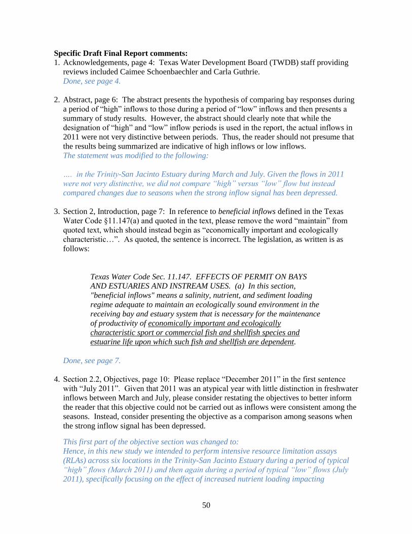
50

Specific Draft Final Report comments: 1. Acknowledgements, page 4: Texas Water Development Board (TWDB) staff providing

reviews included Caimee Schoenbaechler and Carla Guthrie.

Done, see page 4.

2. Abstract, page 6: The abstract presents the hypothesis of comparing bay responses during

a period of ―high‖ inflows to those during a period of ―low‖ inflows and then presents a

summary of study results. However, the abstract should clearly note that while the

designation of ―high‖ and ―low‖ inflow periods is used in the report, the actual inflows in

2011 were not very distinctive between periods. Thus, the reader should not presume that

the results being summarized are indicative of high inflows or low inflows.

The statement was modified to the following:

…. in the Trinity-San Jacinto Estuary during March and July. Given the flows in 2011

were not very distinctive, we did not compare “high” versus “low” flow but instead

compared changes due to seasons when the strong inflow signal has been depressed.

3. Section 2, Introduction, page 7: In reference to beneficial inflows defined in the Texas

Water Code §11.147(a) and quoted in the text, please remove the word ―maintain‖ from

quoted text, which should instead begin as ―economically important and ecologically

characteristic…‖. As quoted, the sentence is incorrect. The legislation, as written is as

follows:

Texas Water Code Sec. 11.147. EFFECTS OF PERMIT ON BAYS

AND ESTUARIES AND INSTREAM USES. (a) In this section,

"beneficial inflows" means a salinity, nutrient, and sediment loading

regime adequate to maintain an ecologically sound environment in the

receiving bay and estuary system that is necessary for the maintenance

of productivity of economically important and ecologically

characteristic sport or commercial fish and shellfish species and

estuarine life upon which such fish and shellfish are dependent.

Done, see page 7.

4. Section 2.2, Objectives, page 10: Please replace ―December 2011‖ in the first sentence

with ―July 2011‖. Given that 2011 was an atypical year with little distinction in freshwater

inflows between March and July, please consider restating the objectives to better inform

the reader that this objective could not be carried out as inflows were consistent among the

seasons. Instead, consider presenting the objective as a comparison among seasons when

the strong inflow signal has been depressed.

This first part of the objective section was changed to:

Hence, in this new study we intended to perform intensive resource limitation assays

(RLAs) across six locations in the Trinity-San Jacinto Estuary during a period of typical

“high” flows (March 2011) and then again during a period of typical “low” flows (July

2011), specifically focusing on the effect of increased nutrient loading impacting

51

phytoplankton community structure. However, given the actual flows in 2011 were not

very distinctive, the results do not reflect a true response to high versus low flows. Rather,

the objective became a comparison of phytoplankton responses between seasons when the

strong inflow signal was suppressed.

5. Section 3.1, Freshwater Inflows, page 11: Please describe the method for reporting inflows

used in the analyses. (See also comment #8, below.) It would be helpful to also report the

sampling dates and most recent inflow volumes preceding each sampling date.

We have dropped all reference to high and low flows and instead refer to March versus

July.

The sampling dates were added to the methods section (Section 3.6).

The most recent inflow volumes preceding each sampling data are shown on Fig. 4. In

terms of volume, we determined the 30 day cumulative total before sampling and added

this information to Section 3.6. We have not gone into detail about why we chose 30 days

in the methods section.

We added:

Sampling occurred from March 15 to 16 2011 and from July 11 to 12 2011. In the 30 day

period preceding these sampling campaigns, a total of 53,240 cfs (105,600 acre-feet) and

54,540 cfs (108,179 acre-feet) were discharged respectively. That is, a similar amounts of

FWI’s preceding the March and July sampling events.

6. Section 3.2, Water Quality, page 11: Please include information on the sampling dates in

March and July. Also, please describe the depth within the water column from which and

how many replicate samples were collected at each station on each sampling trip.

Sampling dates and sampling strategy have been added to Section 3.2.

7. Section 3 various, pages 11 - 16: The Methods section does not describe data analysis

methods. Please describe the methods for statistical analysis.

A description of the statistical analysis which has now been performed is added in Section

3.7.

8. Section 4.2, Results for Freshwater Inflow, page 18: The study attempted to compare bay

responses during a ―high‖ inflow period to those during a ―low‖ inflow period, but actual

inflows in 2011 were suppressed due to drought and thus the two periods were not

distinctive in terms of inflow (e.g., March inflows 45,986 cfs versus July inflows 49,180

cfs). Nonetheless, the report maintains the use of the ―high‖ versus ―low‖ inflow

terminology. Please consider replacing all use of this terminology with a March versus

July designation.

We have dropped all reference to high and low flows and instead refer to March versus

July throughout the document.

52

Inflows from the Trinity River are represented as total discharge (cubic feet per second).

Please describe how the annual values for 2010 and 2011 and the monthly values for

March and July were determined. Please verify the reported values and their units. In

addition, TWDB reports inflows and water volumes in acre-feet; please include this unit

conversion in discussions related to water volume and freshwater inflow.

We added the following to the methods section (section 3.1):

By summing the daily flows provided on the USGS web site, we determined the total

monthly and annual flow from the Trinity River respectively.

And

In order to report flows inflows and water volumes in acre-feet, we used the

conversation factor 1.983471 (Qingguang Lu; TWDB hydrologist), that is, 1 cubic foot

per sec (cfs) for 24 hours = 1.983471 acre-feet. We summed daily flows in acre-feet to

determine the total monthly and annual flow from the Trinity River respectively.

As mentioned above, we have dropped all reference to high and low flows and instead

refer to March versus July throughout the document. Also, the presentation of cfs and

acre-feet throughout is consistent with statements above.

9. Section 4.4, Results for Chl a concentration, page 24: Please clarify the description of

chlorophyll a results in the third sentence. As written, the results refer to the San Jacinto

River basin and the Upper Trinity River basin. However, the intent is that chlorophyll a

differs between the bay location (Upper Galveston Bay, Station 6) influenced by the San

Jacinto River and the bay location (Upper Trinity Bay, Station 1) influenced by the

Trinity River. Please report whether the values are mean values from replicate samples

or a singular value from a single sample.

We have revised the sentences in this section and reported that the values are not means.

10. Section 4.5, Results for Total Suspended Solids, page 24: Please explain how total

sediment loading was estimated from TSS concentrations and report the estimated

loadings. If total sediment loading into the estuary was not estimated, please rephrase

the results statement. Please report whether the values are mean values from replicate

samples or a singular value from a single sample.

Additionally, please provide supporting information for the claim that TSS values were

lower than normal in March and that July values were based on wind induced mixing.

We revised the entire section so that it now reads:

Total sediment loading in the Trinity-San Jacinto Estuary was estimated from

measurements of TSS concentrations (Table 8), that is, the TSS values were used as

indicators of sediment concentrations in the water column. These are only proxies of

loading as TSS values are also influenced by other processes which include but are not

limited to wind induced mixing and resuspension events. The TSS values in Table 8 are

53

typical of low flow periods in the Trinity-San Jacinto Estuary (see Quigg 2010). Given

the unusual flow conditions in 2011, this is not unexpected.

11. Section 4.6, Nutrient Concentrations, page 25: Please include the nutrient acronyms

used in Tables 9 and 10 when reporting nutrient results. Additionally, when reporting

results, please clarify whether significance tests were used to determine differences

among stations. If analyses were conducted to statistically compare station results or to

correlate with river inflows, please report the analyses in the text. If analyses were not

conducted, please provide information to support the claims that a one river provides

more (or less) nutrients than another. Or, please rephrase the results statements to

indicate that data suggests these patterns of nutrient contribution.

Figure legends have been changed to:

Nutrient parameters measured at the fixed stations immediately prior to performing the

RLAs in March 2011. Nitrate (NO3-), HPO4

-(phosphate), silicate (HSiO3

-), ammonium

(NH4+), nitrite (NO2

-), urea, total particulate nitrogen (TN) and total particulate

phosphate (TP) were measured. The following were calculated: Nitrate plus nitrite (NO3-

+ NO2-), dissolved inorganic nitrogen (DIN) and DIN:P.

Statistics have been added were appropriate and we also softened the language.

12. Section 4.8, Resource Limitation Assays, page 29: The first paragraph describes the

categorization of sampling periods as being either ―high‖ inflow or ―low‖ inflow. The

text correctly states that 2011 was not a typical inflow year, with respect to seasonal

inflows, but the last sentence incorrectly states that the sampling periods occurred during

appropriate flow conditions. Moreover, the statement that water quality results differed

between the sampling periods is counter to previous results statements suggesting that

low inflows in March and wind mixing in July created differing results.

Reference to high and low flows is removed as well as the rest of the first paragraph.

Jumping straight into results!

13. Section 4.8, Resource Limitation Assays, page 30 - 33: A significant phytoplankton

response index was identified as measuring >140% of the control, please relate this value

to the discussion of results within the paragraph. Additionally, please report p-values or

other criteria for any significance tests conducted on the results. If no tests were

conducted, please restate the discussion to remove suggestions of ―significant

difference‖.

Done.

14. Section 4.9, Pigment Analysis, page 34: Please state whether the results of the pigment

analysis will be provided to TWDB once available. When are the results expected?

This information has been added. Results are expected no later than March 31.

15. Section 5, Discussion, page 38: Senate Bill 3 regulations have been developed for this

estuary; however, existing water rights are not affected by Senate Bill 3 regulations.

54

Future water rights will be regulated by Senate Bill 3 determinations, but have far less

potential to impact freshwater inflows than existing water rights.

We have modified the text with your assistance.

16. Section 5, Discussion, page 39: The first paragraph on this page states that patterns of N

limitation and P limitation are opposite of previous reports for this estuary. Please

describe the manner in which these patterns are opposite (e.g., the DIN:P and TN:TP

ratios are the opposite or the nutrient limitation patterns are opposite). Also, are these

statements consistent with the discussion presented in the second paragraph on page 39.

This paragraph has been revised to make things clearer and be consistent with rest of

the report.

If data is available from prior studies for nutrient or phytoplankton responses in March

and July at these bay locations, please consider incorporating this information into the

report to better synthesize the information learned from this study.

This is the first year we did the 6 locations, previously we had only done 2 locations so

this kind of comparison is not yet possible.

17. Section 7, Bibliography, pages 41: Please add Espey et al. 2009 and verify all other

referenced literature is included in the bibliography. Please ensure that Bibliography

entries are consistent. For example, some entries state ―et al.,‖ while others list the

names of secondary authors. Preference is to list all authors for a bibliographic entry,

but to use et al. within the text when referencing a document.

Thanks for Espey – thought we have them all.

The bibliography has been made consistent as with the text.

55

Figures and Tables Comments:

1. Section 4.1, Table 2, page 17: Please add units of measure for air temperatures listed in

Table 2.

Done.

2. Section 4.1, Table 3, page 18: Please add units of measure for rainfall listed in Table 3.

Done. Added to table title.

3. Section 4.4, Table 7, page 24: Please include the units of measure for the Chlorophyll a

values presented in the table.

Done. Added to table title.

4. Section 4.4, Table 8, page 24: Please include the units of measure for the Total Suspended

Sediment values presented in the table.

Done. Added to table title.

5. Section 4.6, Tables 9 and 10, page 26: Please provide a written description, either in the

table captions or in the report (Methods or Results sections) of the nutrient acronyms used

in the tables.

Done. Added to table title.

6. Section 4.7, Table 11, page 28: The table presents only data for three stations (1, 3 and 5)

in March and July, not six station as stated in the table caption. Please correct either the

caption or the table.

Done. Caption revised.

56

SUGGESTED CHANGES

Specific Draft Final Report Comments:

1. Sections 2 or 6, Introduction or Conclusion: Please consider adding a brief discussion of

how this particular study will assist in the development of a nutrient budget for the

Galveston Bay system.

Done. A subsection was added to section 2.

2. Sections 4, 5 or 6, Results, Discussion and Conclusion: Please consider rethinking the

results in terms of ―the loss of the seasonal signal of freshwater inflow‖. Essentially, this

study captured the response of the bay when a normally present seasonal inflow is

suppressed. The attempt to present the study as a comparison between a ―high‖ and ―low‖

inflow period may distort true understanding of the results. It would be very informative

to present and discuss the data in terms of ―what happens when the seasonal signal of

inflows is turned off‖. This should be possible by using data collected from previous years

of study when inflows were high during the spring season.

We have addressed this concern in the Results, Discussion and Conclusion.

3. Section 4.7, Phytoplankton Community Composition, page 29: Please consider

mentioning, here or in the Discussion, the red tide event that occurred in late 2011 and the

potential implications of the results of this study on such events occurring in the future.

A paragraph on this was added to this section of the results discussing the bloom.