a proximal technique for computing the karcher mean of
TRANSCRIPT

A proximal technique for computing the Karcher mean of symmetric
positive definite matrices
Ronaldo Malheiros Gregorio∗ and Paulo Roberto Oliveira†
May 20, 2013
Abstract
This paper presents a proximal point approach for computing the Riemannian or intrinsic Karchermean of, n×n, symmetric positive definite (SPD) matrices. Our method derives from proximal pointalgorithm with Schur decomposition developed to compute minimum points of convex functionson SPD matrices set when it is seen as a Hadamard manifold. The main idea of the originalmethod is preserved. However, here, orthogonal matrices are updated as solutions of optimizationsubproblems on orthogonal group. Hence, the proximal trajectory is built on solving iterativelyRiemannian optimization subproblems alternately on diagonal positive definite matrices set andorthogonal group. No Cholesky factorization is made over variables or datum of the problem. Bunchesof numerical experiments, for n = 2, · · · , 10, and illustrations of the computational behavior ofRiemannian gradient descent, proximal point and Richardson-like algorithms are presented at theend.
Keywords. Karcher mean, symmetric positive definite matrices, proximal point algorithm, geodesicconvexity, orthogonal group.
1 Introduction
Denote by Sn++ the, n×n, SPD matrices set. Consider the intrinsic Karcher mean (IKM) problem of,n× n, SPD matrices
minimize 12
m∑i=1
d2(Xi, X),
X ∈ Sn++,
where {X1, · · · , Xm} ⊂ Sn++ is a datum set over any hypothetical or real scenery and d, the Riemanniandistance with respect to Riemannian metric defined by Hessian of the standard logarithmic barrierfunction for Sn++
F (X) = −ln det(X). (1)
Sn++ is an open Lie subgroup of the, n× n, nonsingular matrices set with Riemannian connectionand, as consequence of Corollary 5.10 in [21, p. 220], it has nonpositive curvature everywhere. Therule for Riemannian distance between A,B ∈ Sn++ resulting from the metric defined by Hessian of (1)is given by
d(A,B) =
√√√√ n∑l=1
ln2 λl(A− 1
2BA−12 ), (2)
where λl(A− 1
2BA−12 ) is the lth eigenvalue of A−
12BA−
12 , l = 1, · · · , n.
In the Euclidean sense, means are important tools in statistical process. For instance, let P ={p1, · · · , pm} be a finite subset of any Euclidean vector space. The Euclidean mean µP, defined by
∗Universidade Federal Rural do Rio de Janeiro, Departamento de Tecnologias e Linguagens, Av. Gov. Roberto Silveira, s/n,
Moqueta, Nova Iguacu - CEP 26020-740, RJ, Brazil. This research is supported by FAPERJ. E-mail: [email protected]†Universidade Federal do Rio de Janeiro, Departamento de Eng. de Sistemas e Computacao, Caixa Postal 68511, CEP 21945-970,
Rio de Janeiro, Brazil. E-mail: [email protected]
1

µP = 1m
m∑i=1
pi, the expected value σ2P, with respect to µP, given by σ2
P =
m∑i=1
‖pi − µP ‖22, where ‖ · ‖2
is the usual 2-norm for vectors, and the standard deviation σP =√σ2P are computed to make an error
analysis over P. σ2P and σP represent global error measurements on P.
These ideas can be extended for statistical analysis of tensors. The most well-known applicationbelongs in diffusion tensor (DT ) by magnetic resonance imaging (MRI). In DT −MRI, tensors arerepresented by, 3 × 3, SPD matrices (for further details, see [13]). Statistical analysis is necessary inDT −MRI to treat effects of noises over signal intensities. In general, given a set T = {T1, · · · , Tm} ⊂
Sn++ of tensorial data with Euclidean mean µT = 1m
m∑i=1
Ti, the expected value σ2T, defined by σ2
T =
m∑i=1
Tr{
(Ti − µT)T (Ti − µT)}
, where Tr {·} represents the matrix trace, and the standard deviation
σT =√σ2T are tools computed to estimate the difference between observed tensors at T and the true
diffusion tensor. It remarks that µT can be defined in a continuous differentiable way as the uniquesolution of the Euclidean Karcher mean (EKM) problem
minimize1
2
m∑i=1
‖Ti − µ‖2F
µ ∈ Sn++,
where ‖·‖F is the Frobenius norm of matrices defined by ‖A‖F =√Tr{ATA}, for any matrix A ∈ Rm×n.
Regarded as SPD matrices, tensors can be applied in several research fields. For instance, areas thatemploy this concept include deformation, image analysis, statistical analysis of diffusion tensor data inmedicine, automatic and intelligent control, human detection via classification on the space of SPDmatrices, pattern recognition, speech emotion classification, modeling of cognitive evolution, analysis ofthe multifactorial nature of cognitive aging, modeling of functional brain imaging data and design andanalysis of wireless cognitive dynamic systems (see [8] for further details).
Nowadays, there are developments with tensors specially in DT−MRI working with the Riemannianstructure of Sn++. For instance, see [5], [9], [14] and [27]. In general, let H be a Riemannian manifold ofnonpositive curvature (or Hadamard manifold) and H = {h1, · · · , hm} ⊂ H. Euclidean Karcher meanis extended to Riemannian case in a single way as the unique solution of the problem
minimize1
2
m∑i=1
d2(hi, h)
h ∈ H,
where d is the Riemannian distance defined on H. IKM problem of, n×n, SPD matrices is a particularcase of problem above and it differs from EKM problem by the choice of the geometrical structure ofSn++. Relevant facts listed below are held for IKM problem.
F1. Sn++ is a Hadamard manifold, with respect to the metric given by Hessian of (1).
F2. For any Y ∈ Sn++, g(t) = d2(Y, γ(t)) is a smooth and strictly convex function, for every geodesicsegment γ on Sn++.
F3. IKM problem has unique solution.
It results from F1 and Hadamard theorem that Sn++ is diffeomorphic to Rn(n+1)
2 . In particular, itimplies that geodesic segments joining two points in Sn++ are also unique as in the Euclidean case. Thestrictly convexity and smoothness in F2 follow directly from Theorem 6.1.9 (Semiparallelogram law in
2

Sn++) in [1, p. 207] and Corollary 6.3.2 in [1, p. 218] or, in an alternative way, as a particular case ofTheorem 4.1 in [4, p. 12]. F2 represents the geodesic strictly convexity property of squared Riemanniandistances in Hadamard manifolds regarding the second argument. The unicity in F3 results from F2 andexistence, from completeness of (Sn++, d) as metric space (Proposition 6.2.2 in [1, p. 210]). Geodesicconvexity is discussed with more details in section 3.
The unique solution µ for IKM problem of, n× n, SPD matrices is characterized by
m∑i=1
ln(µ−
12Xiµ−
12
)= 0. (3)
A numerical efficiency measurement for iterative methods to compute µ derives from characterization(3). Let Ψ be an iterative method to solve IKM problem and µΨ, the approach computed by Ψ. Here,
the numerical efficiency of Ψ, represented by EFFΨ, is defined by EFFΨ = ‖m∑i=1
ln
(µ− 1
2Ψ Xiµ
− 12
Ψ
)‖F . It
results from EFFΨ that, under the same computational conditions (same machine, operational system,software for simulations and stopping criteria, for example), a iterative method Ψ1 is numerically moreefficient than other Ψ2 if EFFΨ1 < EFFΨ2 .
In relation to methods, different iterative algorithms in nonlinear programming have been extendedto Riemannian manifolds. These extensions conglobate classical algorithms as gradient, conjugategradient and Newton methods (see [9], [18], [23] and [27] for further details). Sophisticated theoreticalmethods as proximal point algorithms in Hadamard manifolds in [6] and [19] also emphasize this fact.The two late papers are extensions of classical proximal point method introduced in [16] and generalizedto monotone operators in [20].
Let f : Sn++ → R be a geodesic convex function. Given X(0) ∈ Sn++ and a sequence of positive realnumbers {β(k)}k∈N∪{0}, the theoretical proximal point algorithm, as presented in [6, p. 267], generates
a sequence {X(k)}k∈N∪{0} ⊂ Sn++ defined by
X(k+1) = argmin
{f(X) +
β(k)
2d2(X(k), X) : X ∈ Sn++
}, k = 0, 1, · · · , (4)
where infX∈Sn++
{f(X) +β
2d2(X(k), X)} extends the Moreau-Yosida regularization to Riemannian case,
for any β > 0. Theorem 6.1 in [6, p. 269] holds that X(k) converges to a minimum point of f since
{β(k)}k∈N∪{0} satisfies∞∑k=0
1
β(k)= +∞.
In this paper, the proximal point algorithm with Schur decomposition introduced in [11] is fittedto solve the IKM problem. Rules for geodesics on diagonal positive definite (DPD) matrices set, onorthogonal group and for natural gradient of objective function of IKM problem restricted to themare explicitly shown here. Steepest descent algorithm, as presented in [23, p. 117], with Armijo’s linesearch, as in [26, p. 890], is also fitted to solve computationally optimization subproblems in both sets.
Since any information of the objective function of IKM problem restricted to orthogonal group isnot taken into account in the original version of the algorithm, we emphasize that our method differsfrom proximal point algorithm with Schur decomposition as far as orthogonal matrices are updated aslocal solutions of Riemannian optimization subproblems on orthogonal group. No symmetric matrixfactorization is required.
In fact, there are a lot of numerical methods to compute eigenvalues and eigenvectors of symmetricmatrices, such as power method, inverse iteration, Rayleigh quotient iteration, orthogonal iteration (see[10] for further details). However, as it is still under discussion there, a single QR iteration to computeSchur decomposition of symmetric matrices involves O(n3) arithmetic flops and its convergence is linear.Other sophisticated methods compute tridiagonal forms for symmetric matrices inO(n2) arithmetic flops
3

and then the shift idea is applied to reduce them to diagonal form. Since our method escapes fromSchur factorizations, relatively to proximal point algorithm with Schur decomposition, it is O(n3) (orno less than O(n2) and no more than O(n3)) arithmetic flops less expensive per internal iteration.
In addition, it is presented a complexity analysis (with respect to a sequence of accuracy parametersε(k) ≥ 0, k = 0, 1, · · · ) for inexact version, numerical experiments in Sn++ (n = 2, 3, · · · , 10) andillustrations of the computational behavior of Riemannian gradient descent method, as presented in [15,p. 2212], proximal point approach, as described here, and Richardson-like algorithm, as introduced in[3, p. 2].
In section 2, we describe some concepts of Riemannian geometry taking into account geometricalstructures of Sn++ and orthogonal group (On). In section 3, we discuss the classical proximal pointalgorithm on Hadamard manifolds, proximal point algorithm with Schur decomposition for geodesicconvex problems in Sn++, the new orthogonal steps and convergence of internal iterations when applied toIKM problem. In section 4, we present an inexact version of the method and its theoretical complexityanalysis. In section 5, we compute Riemannian gradient flows of the objective function of IKM problemrestricted to diagonal positive definite matrices set and On respectively. Since the aim of this paper ispositioning a proximal point method to compute the Riemannian mean of, n × n, SPD matrices, weimproved on bunches of numerical experiments, for n = 2, · · · , 10, and illustrations that compare thecomputational behavior of proximal point algorithm with Riemannian gradient descent and Richardson-like algorithms, whose Matlab codes can be found in [2].
2 Riemannian aspects of Sn++ and On
2.1 A brief on the Riemannian structure of Sn++
SPD matrices appear in a natural way in several mathematical developments. According to [12],they can be applied in differentiable minimization theory, convexity characterization of differentiablefunctions, variance-covariance matrices, algebraic and trigonometric moments of nonnegative functions,discretization and difference schemes for numerical solution of differential equations. Some theoreticalaspects about Sn++ follow below.
Definition 1 Let Sn be the real symmetric, n × n, matrices set. A matrix X ∈ Sn is said positivedefinite if xTXx > 0, for every x ∈ Rn, x 6= 0.
Another concept intrinsically associated with symmetric matrices is presented in the next definition.
Definition 2 Let Q be a real, n× n, matrix. Q is said orthogonal if QTQ = QQT = I, where I is the,n× n, identity matrix.
Here, notations Dn and Dn++ are used to denote the diagonal, n× n, matrices set and the same setwhose elements have strict positive real numbers in its diagonal respectively.
Theorem 1 (Schur theorem for SPD matrices) Let X ∈ Sn. X ∈ Sn++ iff exist matrices Q ∈ On
and Λ ∈ Dn++ such that X = QΛQT .
Proof. Theorem 8.1.1 in [10, p. 393] assures existence of Q ∈ On and Λ ∈ Dn satisfying X = QΛQT .Since Λ has all eigenvalues of X in its diagonal, it follows by Theorem 7.2.1 in [12, p. 402] that Λ ∈ Dn++.On the contrary, by Sylvester’s law of inertia (Theorem 4.5.8 in [12, p. 223]), if exists Q ∈ On andΛ ∈ Dn++ such that X = QΛQT then X ∈ Sn++.
Theorem 1 makes a characterization for Sn++. Mathematically, Sn++ = {X ∈ Sn|X = QΛQT ;Q ∈On,Λ ∈ Dn++}.
Lemma 1 Let X ∈ Sn and f be a scalar function defined in λi(X), i = 1, · · · , n, where λi(X) is the ith
eigenvalue of X. Then f(X) = Qf(Λ)QT , where f(Λ) ∈ Dn satisfies [f(Λ)]ii = f(λi(X)), i = 1, · · · , n.
4

Proof. Against, Theorem 8.1.1 in [10] assures existence of Q ∈ On and Λ ∈ Dn such that X = QΛQT ,where Λii = λi(X), i = 1, · · · , n. The statement follows as particular case of Corollary 11.1.2 in [10, p.558].
For instance, Lemma 1 implies that eX = QeΛQT for any X ∈ Sn, where Q ∈ On and Λ ∈ Dnsatisfy X = QΛQT , and ln(X) = Qln(Λ)QT , since X ∈ Sn++. There are no difficulties on computingsymmetric and SPD matrices functions.
It is well-known from Real Mathematical Analysis that every bounded sequence of positive realnumbers has as closure points nonnegative real numbers. This implies that every bounded sequencein Sn++ has symmetric matrices with nonnegative eigenvalues as closure points. The closure of Sn++
is called symmetric positive semidefinite matrices set. Sn++ is an open differentiable manifold and itstangent bundle is TSn++ = ∪X∈Sn++
TXSn++ = Sn, where TXSn++ represents the tangent space to Sn++ atX.
The real, n×n, matrices set is a Hilbert space, with respect to Frobenius scalar product defined by
〈A,B〉F = Tr(ATB) =n∑i,j
aijbij and Sn is a Hilbert subspace of it. Frobenius scalar product restricted
to Sn is given by 〈X,Y 〉F = Tr(XY ) (with associated norm ‖X‖F =√Tr(X2)). Since barrier function
(1) is strictly convex, with respect to Euclidean metric (metric resulting from Frobenius scalar product),its Hessian induces an inner product on TXSn++, given by
〈S1, S2〉X = 〈F ′′(X)S1, S2〉F = 〈X−1S1X−1, S2〉F = Tr
{X−1S1X
−1S2
}, (5)
that depends on X ∈ Sn++ in a differentiable way, where S1, S2 ∈ TXSn++ (with associated norm
‖S‖X =
√Tr{
(X−1S)2}
, for any S ∈ TXSn++). Sn++ provided itself with the inner product (5) on
TXSn++ is a Hadamard manifold.According to [17, p. 739], the geodesic on Sn++ satisfying γ(0) = X and γ′(0) = S, for any S ∈
TXSn++, is given by
γ(t) = X12 etX
− 12 SX−
12X
12 , t ∈ R. (6)
In addition, Theorem 6.1.6 in [1, p. 205] establishes the closed rule for geodesic segment γ connectingX to Y . γ is explicitly given by
γ(t) = X12
(X−
12Y X−
12
)tX
12 , t ∈ [0, 1]. (7)
The Riemannian distance (2) results from relation d(X,Y ) =
∫ 1
0‖γ′(t)‖γ(t)dt. It follows from (7) that
the geodesic segment connecting two diagonal positive definite matrices contains only diagonal positivedefinite matrices. So, we conclude that Dn++ is an open subset of Sn++ that contains the geodesic segmentconnecting two of their points, for any pair of points in it.
Definition 3 Let f : Sn++ → R be a function of class C1. The natural (or Riemannian) gradient of f ,denoted by grad f , is a map from Sn++ to Sn that satisfies 〈grad f(X), S〉X = 〈∇f(X), S〉F , for everyS ∈ Sn, where ∇f(X) is the Euclidean gradient of f at X.
Definition 3 is an adaptation of Definition 1.5 in [22, p. 31]. It follows from the inner product (5) that
grad f(X) = X∇f(X)X. (8)
5

2.2 A brief on the Riemannian structure of On
Some statements about On follow naturally from its own definition. Let Q ∈ On. The columns of Q forman orthonormal basis for Rn and |det (Q)| = 1. On is also a Lie subgroup of, n×n, nonsingular matricesset with respect to the matrix product. In this section, we cite Riemannian geometrical concepts on On
necessaries to state our method.The Riemannian structure of On receives especial treatment in [7]. As discussed there, On is a
nonconnected compact manifold that contains a compact connected component. It is known as specialorthogonal group (SOn) and their elements are matrices whose determinant is equal to 1.
For instance, let Q(t) be a smooth path on On, with Q(0) = Q. It follows from Definition 2 that(d
dt|t=0Q(t)T
)Q(0) + Q(0)T
(d
dt|t=0Q(t)
)= (Q′(0))TQ + QTQ′(0) = 0. This implies that TQOn =
{X ∈ Rn×n|XTQ + QTX = 0}. Moreover, the inner product in TQOn coincides with Frobenius scalarproduct for, n × n, matrices. The rule to the geodesic ξ in On, satisfying ξ(0) = Q and ξ′(0) = V , forany V ∈ TQOn, is given by
ξ(t) = exp(tV QT )Q, (9)
where exp(tX) =∞∑k=0
(tX)k
k!. The rule for natural gradient of a function f : On → R, of class C1, at
TQOn is given by
grad f(Q) =1
2(∇f(Q)−Q∇f(Q)TQ), (10)
where ∇f(Q) is the Euclidean gradient of f at Q.
3 IKM problem and proximal point algorithm3.1 Convexity and proximal regularization
In this section, proximal results are discussed with respect to Riemannian convexity in Sn++. All thestatements about Euclidean convexity can be extended in a Riemannian sense for Sn++, since it repre-sents an example of Hadamard manifolds. We recommend [4] for further explanations about geodesicconvexity in Hadamard manifolds. Properties of geodesic convex programs in Riemannian manifolds as,for example, characterization of minimum points to smooth and geodesic convex function and unicityof interior minimum point for smooth and strictly convex function (if it exists) can be found in [25]. Bynow, we are interested in synthesizing extensions of Euclidean convexity properties used by our method.
Definition 4 (Geodesic convex sets and functions) Let C ⊆ Sn++. C is said geodesic convex iffor every X,Y ∈ C, the geodesic segment γ connecting X to Y belongs on C. In addition, g : C → R issaid geodesic (strictly) convex on C if g(γ(t)) is a (strictly) convex function, for every geodesic segmentγ in C.
Lemma 2 Let Y ∈ Sn++. Define fY : Sn++ → R by fY (X) =1
2d2(Y,X). fY is a smooth and geodesic
strictly convex function and its Riemannian gradient is given by
grad fY (X) = −X12 ln(X−
12Y X−
12
)X
12 . (11)
Proof. Since Sn++ is a Hadamard manifold, geodesic strictly convexity and smoothness of fY isheld. Let γX be the geodesic segment on Sn++ connecting Y to X (γX(0) = Y , γX(1) = X andγX(t) ∈ Sn++, ∀t ∈ (0, 1)) and γX , its reparametrization by arc length. From Proposition 4.8 in[22, p. 108] we have that the gradient of dY : Sn++ → R, defined by dY (X) = d(Y,X), is given bygrad dY (X) = γ′X(d(Y,X)) = 1
d(Y,X)γ′X(1). Let W ∈ Sn. Put r(t) = fY (η(t)) = 1
2d2(Y, η(t)), for
any smooth path η in Sn++ tangent to W at η(0) = X. We have that 〈grad fY (X),W 〉X = ddt |t=0
r(t) = 12
[2d(Y, η(t))〈grad dY (η(t)), η′(t)〉η(t)
]|t=0= 〈γ′X(1),W 〉X . Hence, grad fY (X) = γ′X(1). To
finish, define γX(t) = γX(1 − t). It is easily seen that γX is the geodesic segment from X to Y and
6

γ′X(t) = −γ′X(1 − t). This implies that γ′X(1) = −exp−1X Y , where exp−1
X Y is the velocity of γX at X(exp−1
X Y = γ′X(0)). Equality (11) comes from differentiation of (7), with respect to t, at t = 0.It is well-known that differentiable functions in Euclidean spaces are convex iff they satisfy the
gradient’s inequality. This is still guaranteed for geodesic convex function on Hadamard manifolds. Inparticular, the following statement holds it for Sn++.
Lemma 3 Let S ⊆ Sn++ be geodesic convex and g : S→ R, a function of class C1. g is geodesic convexon S iff g(X) ≥ g(Y ) + 〈grad g(Y ), exp−1
Y X〉Y , for every X,Y ∈ S. In addition, g is geodesic strictlyconvex iff the inequality above is strict, for every X 6= Y .
Proof. It follows as a particular case of Theorem 5.1 in [25, p. 78].
Definition 5 Let Y ∈ Sn++. g : Sn++ → R is said 1-coercive at Y if limd(Y,X)→+∞
g(X)
d(Y,X)= +∞.
It remarks that 1-coercivety, under the continuity assumption for g, holds existence of minimumpoints. In fact, definition above implies that, for every sequence {Y (k)}k∈N, such that d(Y, Y (k))→ +∞,g(Y (k)) ≥ d(Y, Y (k)) for k sufficiently great. Therefore, g attains its minimum in a closed geodesic ballaround Y (Bε(Y ) = {X ∈ Sn++|d(Y,X) ≤ ε}, for any ε > 0). Since closed geodesic balls are compact,affirmation at the beginning of the paragraph follows.
Lemma 4 Let g : Sn++ → R be a smooth and geodesic convex function and Y ∈ Sn++. Then (g + βfY )is 1-coercive at Y .
Proof. Since g is differentiable, ∂g(Y ) = {grad g(Y )}, where ∂g(Y ) is the subdifferential of g atY . On the other hand, smoothness and geodesic convexity of g holds Lemma 3. At this point theargumentation follows the same steps of Lemma 4.1 proof’s in [6, p. 266].
Corollary 1 Let f : Sn++ → R be the function given by f(X) =
m∑i=1
fXi(X). For each Y ∈ Sn++ and
β > 0, define (f + βfY ) : Sn++ → R by (f + βfY ) (X) = f(X) + βfY (X). Then both, f and (f + βfY )are smooth and geodesic strictly convex functions, with the second 1-coercive at Y , and their Rieman-
nian gradients are given by grad f(X) = −X12
m∑i=1
ln(X−
12XiX−
12
)X
12 and grad (f + βfY ) (X) =
−X12
m∑i=1
ln(X−
12XiX−
12
)X
12 − βX
12 ln(X−
12Y X−
12
)X
12 respectively.
Proof. It follows from Lemma 2 that f and (f + βfY ) are sums of smooth and geodesic strictly convexfunctions. Hence, f and (f + βfY ) are also smooth and geodesic strictly convex functions. In addition,it follows, from Lemma 4, that (f + βfY ) is 1-coercive at Y . grad f(X) and grad (f + βfY ) (X) followfrom (11).
Proposition 1 Let {X(k)}k∈N∪{0} be the sequence generated by (4). X(k+1) is well-defined and char-acterized by
m∑i=1
ln
(X(k+1)−
12XiX(k+1)−
12
)= −β(k)ln
(X(k+1)−
12X(k)X(k+1)−
12
). (12)
Proof. Since X(k+1) is defined as solution of iteration (4), grad(f + β(k)fX(k)
)(X(k+1)) = 0 (see
Theorem 7.5 in [25, p. 91]). The statement follows from the expression of grad (f + βfY ) in Corollary1 and nonsingularity of X(k+1).
Lemma 5 There is only one solution µ for IKM problem characterized by (3).
Proof. See [1, p. 217].
7

3.2 SDPProx algorithm and new orthogonal steps
Now, the proximal point algorithm in [11, p. 473], named SDPProx algorithm, can be fitted tocompute the intrinsic Karcher mean of, n× n, SPD matrices, since it is defined as the unique solutionof a geodesic strictly convex optimization problem on Sn++. In fact, that algorithm was developed tocompute minimum points of geodesic convex functions defined on Sn++.
Its convergence is held under no assumption of differentiability there because the subdifferentialtheory for geodesic convex function on Hadamard manifolds is already well positioned (see [6] or [25]for further details). It remarks that SDPProx algorithm is a variant of the theoretical proximal pointmethod in Hadamard manifolds, where X(k+1), defined at iteration (4), is iteratively computed in two
recursive phases. For instance, given Q(k)(0) ∈ On and Λ
(k)(0) ∈ Dn++, for any k (k = 0, 1, · · · ), the internal
loop of SDPprox algorithm generates sequences {Q(k)(j)}j∈N∪{0} ⊂ On and {Λ(k)
(j)}j∈N∪{0} ⊂ Dn++ by thefollowing steps
S1. Λ(k)(j+1) = argmin
{φ
(k)(j)(Λ) + β(k)ρI(Λ) : Λ ∈ Dn++
},
S2.(
Λ(k)(j+1), Q
(k)(j+1)
)← Schur
(Q
(k)(j) Λ
(k)(j+1)Q
(k)T
(j)
), j = 0, 1, · · · ,
where φ(k)(j)(Λ) = f
(X(k)
12Q
(k)(j)ΛQ
(k)T
(j) X(k)12
), ρI(Λ) = fX(k)
(X(k)
12Q
(k)(j)ΛQ
(k)T
(j) X(k)12
)and, for any
X ∈ Sn++, Schur (X) returns matrices Λ ∈ Dn++ and Q ∈ On as in Theorem 1. Proposition 2 in [11, p.
475] holds the convergence of the sequence {Y (k)(j) }j∈N∪{0} ⊂ Sn++, defined by the iteration
Y(k)
(j) = X(k)12Q
(k)(j)Λ
(k)(j)Q
(k)T
(j) X(k)12 , (13)
to X(k+1), since Λ(k)(j+1) 6= Λ
(k)(j) , for every j = 0, 1, · · · .
It remarks that SDPProx algorithm replaces iteration 4 by a sequence of problems defined on dia-gonal positive definite matrices set followed by Schur decompositions to update both, diagonal positivedefinite and orthogonal iterated. It represents a reduction of n(n−1)/2 variables per internal iterations
compared to iteration (4). Unfortunately, no practical way to update Q(k)(j) is discussed in [11] if Λ
(k)(j+1) =
Λ(k)(j) . In addition, the updating from Q
(k)(j) to Q
(k)(j+1) in the SDPProx algorithm does not take into
account informations of φ(k)(j) , with respect to the Riemannian structure of On. Moreover, it is easily
seen that ρI does not depend on Q. Next, we will improve a new updating for orthogonal iterated.Firstly, it observes that the rings (Dn,+, ·) and (Rn,⊕,�) (in particular, the fields (Dn++,+, ·) and
(Rn++,⊕,�)) have the same algebraic structure in sense of the ring isomorphism diag : (Dn,+, ·) →(Rn,⊕,�) defined by diag(Λ) = (Λ11, · · · ,Λnn)T , where Rn represents the Euclidean vector space ofdimension n, + and ·, the standard addition and product of matrices and ⊕ and �, the standardaddition and Hadamard product of vectors given by x � y = (x1y1, · · · , xnyn)T , for any x, y ∈ Rn (inparticular, Rn++ represents the positive orthant of Rn).
Remark 1 For simplicity, the capital letter Λ is employed to represent diagonal matrices and the cor-responding small letter λ, for vectors whose components are diagonal elements of Λ in the order thatthey appear in its diagonal.
Let φ(k) : Rn++ ×On → R be the function defined by
φ(k)(λ,Q) = f
(X(k)
12QΛQTX(k)
12
)=
1
2
m∑i=1
d2
(Xi, X(k)
12QΛQTX(k)
12
). (14)
Based on these facts, Q(k)(j+1) is defined in an alternative way as a minimizer of φ(k)(λ
(k)(j+1), ·), since
the minimizer set of φ(k)(λ(k)(j+1), ·) on On is nonempty (notice that φ(k)(λ
(k)(j+1), ·) is continuous on On
8

and itself is compact). The alternative version for SDPProx algorithm, originally called by proximalpoint algorithm here, rewrites S1 as
λ(k)(j+1) = argmin
{φ(k)(λ,Q
(k)(j)) + β(k)ρI(λ) : λ ∈ Rn++
}, (15)
and it replaces S2 by
Q(k)(j+1) ∈ argmin
{φ(k)(λ
(k)(j+1), Q) : Q ∈ On
}, j = 0, 1, · · · . (16)
3.3 Internal convergence analysis
Proposition 2 Let {Λ(k)(j)}j∈N∪{0} and {Q(k)
(j)}j∈N∪{0} be sequences generated by (15) and (16) respe-
ctively. Set Y(k)
(j) as in (13) and Y(k)
(j+1) = X(k)12Q
(k)(j)Λ
(k)(j+1)Q
(k)T
(j) X(k)12 . Then, (f + fX(k))
(Y
(k)(j)
)≥
(f + fX(k))(Y
(k)(j+1)
)+ 1
2d2(Y
(k)(j) , Y
(k)(j+1)
), for every j ∈ N ∪ {0}.
Proof. In fact, it follows by Lemma 4 in [11, p. 474] that
d2(
Λ(k)(j) ,Λ
(k)(j+1)
)+ d2
(Λ
(k)(j+1), I
)− 2
β(k)
(φ(k)
(Λ
(k)(j) , Q
(k)(j)
)− φ(k)
(Λ
(k)(j+1), Q
(k)(j)
))≤ d2
(Λ
(k)(j) , I
).
Multiplying inequality above byβ(k)
2, we have that
φ(k)(
Λ(k)(j+1), Q
(k)(j)
)+β(k)
2d2(
Λ(k)(j+1), I
)+β(k)
2d2(
Λ(k)(j) ,Λ
(k)(j+1)
)≤ φ(k)
(Λ
(k)(j) , Q
(k)(j)
)+β(k)
2d2(
Λ(k)(j) , I
).
Since the Riemannian distance (2) is invariant under isometries (see Lemma 6.1.1 in [1, p. 201]),
applying the isometry ΓQ
(k)T
(j)X(k)
12
: Sn++ → Sn++, given by ΓQ
(k)T
(j)X(k)
12
(Y ) = X(k)12Q
(k)(j)Y Q
(k)T
(j) X(k)12 ,
and definition of φ(k) in the last inequality, we have that
f(Y
(k)(j)
)+ fX(k)
(Y
(k)(j)
)≥ f
(Y
(k)(j+1)
)+ fX(k)
(Y
(k)(j+1)
)+
1
2d2(Y
(k)(j) , Y
(k)(j+1)
). (17)
On the other hand, f(Y
(k)(j+1)
)= f
(X(k)
12Q
(k)j Λ
(k)(j+1)Q
(k)T
(j) X(k)12
)= φ
(λ
(k)(j+1), Q
(k)(j)
)≥ φ
(λ
(k)(j+1), Q
(k)(j+1)
)= f
(X(k)
12Q
(k)(j+1)Λ
(k)(j+1)Q
(k)T
(j+1)X(k)
12
)= f
(Y
(k)(j+1)
)and fX(k)
(Y
(k)(j+1)
)= fX(k)
(X(k)
12Q
(k)(j)Λ
(k)(j+1)Q
(k)T
(j) X(k)12
)= 1
2d2
(X(k), X(k)
12Q
(k)(j)Λk(j+1)Q
(k)T
(j) X(k)12
)= 1
2
n∑l=1
ln2θl
(Q
(k)(j)Λ
(k)(j+1)Q
(k)T
(j)
)=
1
2
n∑l=1
ln2θl
(Λ
(k)(j+1)
)=
1
2
n∑l=1
ln2θl
(Q
(k)(j+1)Λ
(k)(j+1)Q
(k)T
(j+1)
)= 1
2d2
(X(k), X(k)
12Q
(k)(j+1)Λ
(k)(j+1)Q
(k)T
(j+1)X(k)
12
)= fX(k)
(X(k)
12Q
(k)(j+1)Λ
(k)(j+1)Q
(k)T
(j+1)X(k)
12
)= fX(k)
(Y
(k)(j+1)
). So, we conclude that
f(Y
(k)(j+1)
)≥ f
(Y
(k)(j+1)
)and fX(k)
(Y
(k)(j+1)
)= fX(k)
(Y
(k)(j+1)
). (18)
Replacing both relations at (18) in the inequality (17), the statement follows.
Corollary 2 If Λ(k)(j+1) 6= Λ
(k)(j) then
(f + fX(k)) (Y(k)
(j) ) > (f + fX(k)) (Y(k)
(j+1)). (19)
9

Proof. Since Λ(k)(j+1) 6= Λ
(k)(j) , 0 < d
(Λ
(k)(j+1),Λ
(k)(j)
)= d
(Y
(k)(j) , Y
(k)(j+1)
). So, inequality (19) results from
Proposition 2.
Corollary 3 Suppose that the hypothesis of Corollary 2 breaks. If φ(k)(λ
(k)(j) , Q
(k)(j+1)
)< φ(k)
(λ
(k)(j) , Q
(k)(j)
)then inequality (19) is still held.
Proof. Since the hypothesis of Corollary 2 is not true, the equality Λkj+1 = Λkj implies that Y(k)
(j+1) =
Y(k)
(j) and, consequently, d2(Y
(k)(j) , Y
(k)(j+1)
)= 0. However, φ(k)
(λ
(k)(j+1), Q
(k)(j+1)
)= φ(k)
(λ
(k)(j) , Q
(k)(j+1)
)<
φ(k)(λ
(k)(j) , Q
(k)(j)
). This implies that f
(Y
(k)(j+1)
)< f
(Y
(k)(j)
). Taking into account the latest inequality
and the equality in (18), inequality (19) still follows.
Proposition 3 Let {Λ(k)(j)}j∈N∪{0} and {Q(k)
(j)}j∈N∪{0} be the sequences generated by (15) and (16) re-spectively. Suppose that the following two statements are held
(i) Λ(k)(j+1) = Λ
(k)(j) ,
(ii) φ(k)(λ
(k)(j) , Q
(k)(j)
)= φ(k)
(λ
(k)(j) , Q
(k)(j+1)
)for every minimizer Q
(k)(j+1) of φ(k)
(λ
(k)(j) , ·
).
Then Y(k)j = X(k+1).
Proof. By contradiction, suppose that Y(k)
(j) 6= X(k+1). Since(f + β(k)fX(k)
)is geodesic strictly convex,
for every δ > 0, the normal ball around Y(k)
(j) , given by Bδ
(Y
(k)(j)
)={Y ∈ Sn++ : d
(Y
(k)(j) , Y
)< δ}
,
contains at least one point Yδ such that(f + β(k)fX(k)
)(Yδ) <
(f + β(k)fX(k)
)(Y
(k)(j)
)(20)
(if this is not true, Y(k)
(j) would be a local minimum of(f + β(k)fX(k)
)and, as consequence of its geodesic
strict convexity, Y(k)
(j) = X(k+1)). By Theorem 1 and taking into account that ΓX(k)
12
(Y ) = X(k)12 Y X(k)
12
is an isometry on Sn++, there are matrices Qδ ∈ On and Λδ ∈ Dn++ such that Yδ = X(k)12QδΛδQ
Tδ X
(k)12 .
Now, we can divide the proof in two cases. Firstly, admit that Qδ = Q(k)(j) . It follows from inequality
(20) that Λδ 6= Λ(k)(j) and φ(k)
(λδ, Q
(k)(j)
)+β(k)ρI (λδ) = φ(k) (λδ, Qδ) +β(k)ρI (λδ) =
(f + β(k)fX(k)
)(Yδ)
<(f + β(k)fX(k)
) (Y
(k)(j)
)= φ(k)
(λ
(k)(j) , Q
(k)(j)
)+β(k)ρI
(λ
(k)(j)
). It contradicts (i). Now, suppose that Qδ 6=
Q(k)(j) . In addition, admit that Λδ 6= Λ
(k)(j) . Let γ be the geodesic segment from Y
(k)(j) to Yδ. We have that(
f + β(k)fX(k)
)(γ(t)) < (1− t)
(f + β(k)fX(k)
) (Y
(k)(j)
)+ t(f + β(k)fX(k)
)(Yδ) <
(f + β(k)fX(k)
) (Y
(k)(j)
),
for every t ∈ (0, 1). In particular,(f + β(k)fX(k)
) (γ(
12
))<(f + β(k)fX(k)
) (Y
(k)(j)
). On the other
side, against by Theorem 1 and the isometry ΓX(k)
12
, for every t ∈ (0, 1) there are Q(t) ∈ On and
Λ(t) ∈ Dn++, such that γ(t) = X(k)12Q(t)Λ(t)QT (t)X(k)
12 . Setting Q(0) = Q
(k)(j) , Λ(0) = Λ
(k)(j) , Q(1) = Qδ
and Λ(1) = Λδ, we have that Q(t) and Λ(t) are paths in On and Dn++ from Q(k)(j) to Qδ and from Λ
(k)(j) to
Λδ, respectively. Set Yδ = X(k)12QδΛ
(k)(j)Q
Tδ X
(k)12 . By Semiparallelogram law,
d2(γ
(1
2
), Yδ
)≤ 1
2d2(Y
(k)(j) , Yδ
)+
1
2d2(Yδ, Yδ
)− 1
4d2(Y
(k)(j) , Yδ
)<
1
2d2(Y
(k)(j) , Yδ
)+
1
2d2(Yδ, Yδ
). (21)
Define c(t) = X(k)12Q(t)Λ
(k)(j)Q
T (t)X(k)12 , t ∈ [0, 1]. Since Q(t) ∈ On, for every t ∈ [0, 1], c(t) is a path
on Sn++ from Y(k)
(j) to Yδ. Without loss of generality we can assume that δ > d(Y
(k)(j) , Yδ
)≥ d
(Yδ, Yδ
)10

Figure 1: Geodesic segment γ, from Y(k)(j)
to Yδ, and the path c, from Y(k)(j)
to Yδ.
(if this is not true we can choose t, t ∈ (0, 1) such that δ > d(Y
(k)(j) , c(t)
)≥ d
(γ(t), c(t)
)and we can
replace Yδ by γ(t) and Yδ by c(t). See figure 1). Replacing it in (21), we have that d(γ(
12
), Yδ)<
d(Y
(k)(j) , Yδ
). Hence, for δ > 0 sufficiently small, the continuity of f implies that
(f + β(k)fX(k)
)(Yδ) <(
f + β(k)fX(k)
) (Y
(k)(j)
)or, equivalently, φ(k)(λ
(k)(j) , Qδ) + β(k)ρI(λ
(k)(j)) < φ(k)(λ
(k)(j) , Q
(k)(j)) + β(k)ρI(λ
(k)(j)).
This implies that φ(k)(λ(k)(j) , Qδ) < φ(k)(λ
(k)(j) , Q
(k)(j)). It contradicts (ii). To finish, if Λδ = Λ
(k)(j) then
Yδ = Yδ. So, we conclude that Yδ is the last point of c(t). Against, it contradicts (ii).
4 Inexact version and its complexity4.1 Inexact algorithm
It remarks that grad f(X(k+1)
)= −β(k)grad fX(k)
(X(k+1)
), since X(k+1) is defined as the solution of
iteration (4) (remmember that grad(f + β(k)fX(k)
) (X(k+1)
)= 0). Under Lemmas 2 and 3, X(k+1)
satisfies f(X) > f(X(k+1))+β(k)〈X(k+1)12 ln
(X(k+1)−
12X(k)X(k+1)−
12
)X(k+1)
12 , exp−1
X(k+1)X〉X(k+1) , for
every X ∈ Sn++, X 6= X(k+1). Let ε(k) ≥ 0, k = 0, 1, · · · , be a sequence of accuracy parameters andX(0) ∈ Sn++. In despite of the exact version, in the inexact algorithm we weaken the late inequality.
Algorithm 1 (Inexact proximal point algorithm) Given X(0) ∈ Sn++ and β(0), ε(0) > 0.1. k = 0.2. Computing X(k+1) ∈ Sn++ satisfying
f(X) ≥ f(X(k+1))+β(k)〈X(k+1)12 ln
(X(k+1)−
12X(k)X(k+1)−
12
)X(k+1)
12 , exp−1
X(k+1)X〉X(k+1)−ε(k), (22)
for every X ∈ Sn++.3. Updating k and returning to 2.
Inequality (22) means that β(k)X(k+1)12 ln
(X(k+1)−
12X(k)X(k+1)−
12
)X(k+1)
12 ∈ ∂ε(k)f
(X(k+1)
), i.
e., it is a ε(k)-subgradient to f at X(k+1), for k = 0, 1, · · · . This is the assumption of the ine-xact version of SDPProx algorithm (see ε(k)-subdifferential relation in [11, p. 475]). For instance,the ε-subdifferential of a function g : Sn++ → R at Y ∈ Sn++, represented by ∂εg(Y ), is definedby ∂εg(Y ) =
{S ∈ Sn|g(X) ≥ g(Y ) + 〈S, exp−1
Y X〉Y − ε,∀X ∈ Sn++
}. Note that in the exact version
grad f(X(k+1)) = β(k)X(k+1)12 ln
(X(k+1)−
12X(k)X(k+1)−
12
)X(k+1)
12 , k = 0, 1, · · · . The exact proximal
point algorithm is a particular case of this inexact version, since ∂ε(k)f(Y ) ⊃ ∂f(Y ) = {grad f(Y )}, forevery Y ∈ Sn++, where ∂f(Y ) represents the subdifferential of f at Y , (if ε(k) = 0, for every k = 0, 1, · · · ,then ∂ε(k)f
(X(k+1)
)= ∂f
(X(k+1)
)= {grad f
(X(k+1)
)} and inexact version resumes itself to exact
proximal point method).
11

Theorem 2 (Convergence of the inexact version) Suppose that X(k+1) satisfies (22), for everyk = 0, 1, · · · . If the following assertments are held for β(k) and ε(k)
∞∑k=0
1
β(k)= +∞,
∞∑k=0
ε(k) < +∞,∞∑k=0
ε(k)
β(k)< +∞, (23)
then X(k) → µ.
Proof. It follows directly from Theorem 2 in [11, p. 477].
We still have that d2(X(k+1), X(k)) = 〈exp−1X(k+1)X
(k), exp−1X(k+1)X
(k)〉X(k+1), where exp−1X(k+1)X
(k) =
X(k+1)12 ln
(X(k+1)−
12X(k)X(k+1)−
12
)X(k+1)
12 . Replacing X(k) at (22) it follows that X(k+1) satis-
fies d2(X(k+1), X(k)) ≤ε(k) + f
(X(k)
)− f
(X(k+1)
)β(k)
, k = 0, 1, · · · . On the other hand, f(X(k)
)≥
minY ∈Sn++
{f(Y ) + β(k)f(X(k))(Y )
}≥ f
(X(k+1)
), since fX(k)
(X(k)
)= 0 and fX(k) (Y ) ≥ 0, for every
Y ∈ Sn++. Algorithmically, we repeat iterations (15) and (16) in this order while d(Y
(k)(j+1), X
(k))>√√√√ε(k) + f
(X(k)
)− f
(Y
(k)(j+1)
)β(k)
. When this condition is false we stop both steps and we choose Y(k)
(j+1)
to be X(k+1).
4.2 Complexity
In the inexact version, ε(k) is previously established for each iteration of the method. The number ofiterations necessary to get a ε-solution for IKM problem, for any tolerance ε > 0, can be estimatedunder a certain assumption. However, this is not discussed in a practical way here. The following resultimproves on it.
Proposition 4 Let{X(k)
}k∈N∪{0} be a sequence generated by (22). Suppose that exists α(k) ∈ (0, α],
for any α ∈ (0, 1), such that
ε(k)
β(k)≤ α(k)d2
(X(k+1), X(k)
), ∀k = 0, 1, · · · , (24)
then2
β(k)ε(k)
(1
α− 1
)≤ d2
(X(k), µ
), for every k = 0, 1, · · · .
Proof. Since{X(k)
}k∈N∪{0} satisfies (22), Lemma 7 in [11, p. 476] is held. So, we have that
d2(X(k+1), X
)≤ d2
(X(k), X
)− d2
(X(k), X(k+1)
)+
2
β(k)
(f(X)− f
(X(k+1)
))+
2
β(k)ε(k),
for every X ∈ Sn++. In particular, for X = µ and taking into account inequality (24), we have that
d2(X(k), µ
)≥ d2
(X(k+1), µ
)+ d2
(X(k), X(k+1)
)+
2
β(k)
(f(X(k+1)
)− f(µ)
)− 2
β(k)ε(k)
≥ d2(X(k+1), µ
)+
ε(k)
β(k)α(k)+
2
β(k)
(f(X(k+1)
)− f(µ)
)− 2
β(k)ε(k)
≥ d2(X(k+1), µ
)+
2
β(k)
(f(X(k+1)
)− f(µ)
)+
2
β(k)ε(k)
(1
α− 1
)≥ 2
β(k)ε(k)
(1
α− 1
).
12

Corollary 4 Let ε > 0 be any tolerance. If β(k) = β, ε(k) =ε(0)
τk, k = 0, 1, · · · , for any β > 0 and
τ > 1, and inequality (24) is held for every k then at least
dlog(2ε(0)(1− α)
)− log(βαε)
log(τ)e
iterations are necessary to have d(X(k), µ
)≤ ε, where dte represents the ceiling of t for any t ∈ R.
Proof. Firstly, note that β(k) = β and ε(k) =ε(0)
τk, k = 0, 1, · · · , satisfy (23). Put d
(X(k), µ
)≤ ε. From
Proposition 4, we have that τk ≥ 2ε(0)(1− α)
βαε. Therefore,
k ≥log(2ε(0)(1− α)
)− log(βαε)
log(τ).
5 Riemannian gradient flows5.1 Gradient flows on Dn
++
Since this work reports to a differentiable Riemannian approach for intrinsic Karcher mean of, n × n,SPD matrices, one question emerges naturally: how can rules for Riemannian gradients of φ(k), asdefined in (14), with respect to λ and Q, be computed? The answer comes from Riemannian structuresof Sn++, restricted to Dn++, and On, both discussed in section 2.
Proposition 5 Set Q ∈ On. φ(k)(·, Q) : Rn++ → R is geodesic strictly convex and smooth and
gradλ φ(k)(λ,Q) = λ�
(∇λφ(k)(λ,Q)
)� λ, (25)
where ∇λφ(k)(λ,Q) is the Euclidean gradient of φ(k), with respect to λ, at (λ,Q).
Proof. Geodesic strict convexity of φ(k)(·, Q) follows from Lemma 2 in [11, p. 472] since Rn++ is isomor-
phic to Dn++. φ(k) is explicitly given by φ(k)(λ,Q) = 12
m∑i=1
n∑l=1
ln2θl
(Xi−
12X(k)
12QΛQTX(k)
12Xi−
12
),
where θl is the lth eigenvalue of Xi−12X(k)
12QΛQTX(k)
12Xi−
12 . Denote by φ(k)i the ith parcel of φ(k).
φ(k)i is given by φ(k)i(λ,Q) =∑n
l=1 ln2θl
(Xi−
12X(k)
12QΛQTX(k)
12Xi−
12
). Set W (k)i = Xi−
12X(k)
12Q.
It is easily seen that W (k)i is nonsingular, W (k)Ti = QTX(k)12Xi−
12 and W (k)Ti ΛW (k)i is a SPD ma-
trix, since Λ ∈ Dn++ (see against Theorem 4.5.8 in [12]). φ(k)i can be rewritten as φ(k)i(λ,Q) =
12
n∑l=1
ln2θl
(W (k)iΛW (k)Ti
)=
1
2
n∑l=1
ln2θl
(W (k)Ti W (k)iΛ
). Setting A(k)i = W (k)Ti W (k)i , it follows that
A(k)i ∈ Sn++ and φ(k)i(λ,Q) = 12d
2(A(k)−1i ,Λ), since W (k)i is nonsingular and A(k)iΛ, similar to
A(k)12i ΛA(k)
12i . So, we conclude that the ith parcel of φ(k) is geodesic strictly convex and smooth. The
Riemannian gradient of φ(k)i , with respect to λ, can be computed in alternative way based on Rieman-nian relation (8). It is easily seen that, in the vector form, the Riemannian gradient of φ(k)i is given bygradλ φ
(k)i(λ,Q) = λ�∇λφ(k)i(λ,Q)� λ, where ∇λφ(k)i(λ,Q) is the Euclidean gradient of φ(k)i , with
respect to λ, at (λ,Q). Since ∇λφ(k)(λ,Q) =
n∑i=1
∇λφ(k)i(λ,Q), proposition follows.
φ(k)i can still be rewritten in a compact form as φ(k)i(λ,Q) = 12
n∑l=1
ln2θl(λ,Q), where θ(λ,Q) ∈ Rn++
is the vector that contains all eigenvalues of Xi−12X(k)
12QΛQTX(k)
12Xi−
12 arranged in increasing order.
13

According to [24, p. 166], a better approximation based in an extrapolation method to the lth componentof ∇λφ(k)i(λ,Q) can be numerically computed by the relation
φ(k)i(λ+ hel, Q)− φ(k)i(λ− hel, Q)
h,
where el is the lth vector of the canonic base of Rn and h > 0 sufficiently small.The regularization ρI(Λ) = d2(I,Λ) can also be written as a function from Rn++ to R. It is easily
seen that ρI(λ) = 12
n∑l=1
ln2λl. Hence, the Euclidean gradient of ρI is given by ∇ρI(λ) = ln(λ) � λ−1,
where ln(λ) and λ−1 are vectors in Rn whose lth component are ln(λl) and1
λl, respectively. Against,
applying the Riemannian relation (8), in the vector form, we conclude that
grad ρI(λ) = λ� ln(λq). (26)
The geodesic rule (6) restricted to Dn++, in the vector form, can be rewritten as
γ(t) = λ� etλ−1�s, (27)
for any vector s ∈ Rn, where ex = (ex1 , · · · , exn)T , for x ∈ Rn.
5.2 Gradient flows on On
Now, set λ ∈ Rn++. We are interested in the Riemannian gradient of φ(k), with respect to Q on theRiemannian structure of On. Relation (10) shows how to compute gradQ φ(k)(λ,Q) ∈ TQOn. Hence,we need to obtain the rule of the Euclidean gradient of φ(k), with respect to Q. Since φ(k)(λ,Q) =m∑i=1
φ(k)i(λ,Q), it is sufficient to compute the Euclidean gradient of φ(k)i , with respect to Q. It results
that ∇Qφ(k)(λ,Q) =m∑i=1
∇Qφ(k)i(λ,Q).
Lemma 6 Let A,B : R→ Rn×n be differentiable paths. Then, [A (t)B (t)]′ = A′ (t)B (t) +A (t)B′ (t).
Proof. Denote C (t) , D (t) e E (t) ∈ Rn×n, t ∈ R by A (t)B (t), A′ (t)B (t) e A (t)B′ (t), respectively.Since A (t) and B (t) are differentiable paths, all elements clq(t), l, q = 1, · · · , n of C (t) are differentiablescalar functions with respect to t and
c′lq (t) =
(n∑p=1
alp (t) bpq (t)
)′=
(n∑p=1
a′lp (t) bpq (t)
)+
(n∑p=1
alp (t) b′pq (t)
)= dlq (t) + elq (t). Therefore,
C ′ (t) = D (t) + E (t) and the statement follows.
Proposition 6 Let Q : R→ On be be a differentiable path. Set
R(k)i (t) = Xi−12X(k)
12Q (t) ΛQ (t)T X(k)
12Xi−
12
and g (t) = 12Tr
{ln(R(k)i (t)
)2}. Then the derivative of g, with respect to t, is given by
g′ (t) = 2
⟨Q′ (t) , X(k)
12Xi−
12 ln
(R(k)i(t)
)(R(k)i(t)
)−1Xi−
12X(k)
12Q (t) Λ
⟩F
.
14

Proof. Since Xi−12X(k)
12Q(t) is nonsingular and Λ ∈ Dn++, R(k)i(t) is symmetric positive definite, for
every t ∈ R. Proposition 2.1 in [17] establishes that g′ (t) = Tr{
ln(R(k)i (t)
) (R(k)i (t)
)−1 (R(k)i (t)
)′}and, according to Lema 6,(
R(k)i (t))′
= Xi−12X(k)
12Q′ (t) ΛQ (t)T X(k)
12Xi−
12 +Xi−
12X(k)
12Q (t) ΛQ′ (t)T X(k)
12Xi−
12 .
This implies that g′ (t) =
= Tr
{ln(R(k)i (t)
) (R(k)i (t)
)−1Xi−
12X(k)
12Q′ (t) ΛQ (t)T X(k)
12Xi−
12
}+Tr
{ln(R(k) (t)
) (R(k)i (t)
)−1Xi−
12X(k)
12Q (t) ΛQ′ (t)T X(k)
12Xi−
12
}= Tr
{ΛQ (t)T X(k)
12Xi−
12 ln
(R(k)i (t)
) (R(k)i (t)
)−1Xi−
12X(k)
12Q′ (t)
}+Tr
{X(k)
12Xi−
12 ln
(R(k)i (t)
) (R(k)i (t)
)−1Xi−
12X(k)
12Q (t) ΛQ′ (t)T
}= Tr
{ΛQ (t)T X(k)
12Xi−
12 ln
(R(k)i (t)
) (R(k)i (t)
)−1Xi−
12X(k)
12Q′ (t)
}+Tr
{Q′ (t)T X(k)
12Xi−
12 ln
(R(k)i (t)
) (R(k)i (t)
)−1Xi−
12X(k)
12Q (t) Λ
}= Tr
{ΛQ (t)T X(k)
12Xi−
12 ln
(R(k)i (t)
) (R(k)i (t)
)−1Xi−
12X(k)
12Q′ (t)
}+Tr
{ΛQ (t)T X(k)
12Xi−
12(R(k)i (t)
)−1ln(R(k)i (t)
)Xi−
12X(k)
12Q′ (t)
}=
⟨Q′ (t) , X(k)
12Xi−
12(R(k)i (t)
)−1ln(R(k)i (t)
)Xi−
12X(k)
12Q (t) Λ
⟩F
+
⟨Q′ (t) , X(k)
12Xi−
12 ln
(R(k)i (t)
) (R(k)i (t)
)−1Xi−
12X(k)
12Q (t) Λ
⟩F
.
The first equality above follows from the substitution of(Rki (t)
)′in g′ (t). The second, third and
fourth equalities are consequence of similar transformation, Tr (AB) = Tr (BA) and Tr (A) = Tr(AT),
respectively. The last equality follows from the definition of Frobenius scalar product. Let Q(k)i : R→On and Λ(k)i : R → Dn++ be paths satisfying R(k)i (t) = Q(k)i (t) Λ(k)i (t)Q(k)Ti (t). So,
(R(k)i (t)
)−1=
Q(k)i (t)(Λ(k)i (t)
)−1Q(k)Ti (t) and ln
(R(k)i (t)
)= Q(k)i (t) ln
(Λ(k)i (t)
)Q(k)Ti (t). Hence
ln(R(k)i (t)
) (R(k)i (t)
)−1= Q(k)i (t) ln
(Λ(k)i (t)
)Q(k)Ti (t)Q(k)i (t)
(Λ(k)i (t)
)−1Q(k)Ti (t)
= Q(k)i (t) ln(Λ(k)i (t)
) (Λ(k)i (t)
)−1Q(k)Ti (t)
= Q(k)i (t)(Λ(k)i (t)
)−1ln(Λ(k)i (t)
)Q(k)Ti (t)
= Q(k)i (t)(Λ(k)i (t)
)−1Q(k)Ti (t)Q(k)i (t) ln
(Λ(k)i (t)
)Q(k)Ti (t)
=(R(k)i (t)
)−1ln(R(k)i (t)
).
This means that ln(R(k)i (t)
)and
(R(k)i (t)
)−1commute and the statement follows.
φ(k)i can also be written in terms of Frobenius scalar product as
φ(k)i(λ,Q) =1
2Tr
{ln
(Xi−
12X(k)
12QΛQTX(k)
12Xi−
12
)2}.
The relation between g and φ(k)i is given by g(t) = φ(k)i(λ,Q(t)), for any differentiable path Q(t)on On. It derives from relation before that g′(t) = 〈∇Qφ(k)i(λ,Q(t)), Q′(t)〉F . Proposition 6 and the
latest equality for g′ imply that ∇Qφ(k)i(λ,Q) = 2X(k)12Xi−
12 ln
(R(k)i(Q)
) (R(k)i(Q)
)−1Xi−
12X(k)
12QΛ,
for any Q ∈ On, where R(k)i(Q) = Xi−12X(k)
12QΛQTX(k)
12Xi−
12 . Since φ(k)(λ,Q) =
m∑i=1
φ(k)i(λ,Q),
15

it follows that ∇Qφ(k)(λ,Q) = 2
m∑i=1
X(k)12Xi−
12 ln
(R(k)i(Q)
)(R(k)i(Q)
)−1Xi−
12X(k)
12QΛ. Replacing
(R(k)i(Q)
)−1in the equality before we have that ∇Qφ(k)(λ,Q) = 2
m∑i=1
P (k)i(Q)Q, where P (k)i(Q) =
X(k)12Xi−
12 ln
(R(k)i(Q)
)Xi
12X(k)−
12 . Finally, replacing the late equality in (10) we conclude that the
Riemannian gradient of φk with respect to Q, at TQOn, is given by
gradQ φ(k) (λ,Q) =
(m∑i=1
P (k)i − P (k)Ti
)Q, (28)
6 Simulations and conclusions6.1 Numerical experiments and computational comparisons between proximal point,
Richardson-like and geodesic gradient algorithms
In this section are presented numerical experiments with inexact proximal point algorithm. All resultsare compared with others obtained by geodesic gradient and Richardson-like algorithm. Simulationswere made automatically in a workstation Xeon E3 1270V2 3.50 GHz 8MB, Linux and routines wereimplemented in Matlab, version R2012a.
Sequences {β(k)}k∈N∪{0} and {ε(k)}k∈N∪{0} were set as in Corollary 4. In addition, we set β = 10−6,
ε(0) = 10−16, τ = 1.5625, X(0) = Q(k)(0) = Λ
(k)(0) = I, k = 0, 1, · · · . We still stopped both steps (15)
and (16) when d(Y
(k)(j+1), X
(k))≤
√ε(k)
β(k), since it attempts the stopping criteria discussed at the end of
Section 4.1.Tables 1 and 2 present procedures that converts a set R = {R1, · · · , Rm} of m, n × n, nonzero
real pseudo-random matrices in a set X = {X1, · · · , Xm} of m, n× n, SPD matrices. Pseudo-randommatrices Ri, i = 1, · · · ,m, were generated in Matlab ambient by syntax Ri = rand(n)− rand(n). Thefirst table can be found in [3, p. 9] and it generates SPD matrices whose eigenvalues belong on theinterval (0, 1], where λ1, λn represent the largest and the smallest eingenvalue of Xi and cr, a conditionnumber previously established.
for i = 1 until m doXi ← RTi Ri;
Xi ← Xi −cr · λn − λ1cr − 1
· I;
Xi ←1
λnXi;
end,
Table 1: Normalized matrices set.
for i = 1 until m do
Xi ←Ri +RTi
2;
Xi ← eXi ;end,
Table 2: Exponential matrices set.
Since expressions for geodesics and Riemannian gradients in On and Dn++ are explicitly known (seerules (9), (25), (26), (27) and (28)), we employ the geodesic gradient method with Armijo’s line search
as presented in [26] to compute Λ(k)(j+1) and Q
(k)(j+1). We emphasize that stating an implementable and
feasible proximal point method to compute the Riemannian mean of, n × n, SPD matrices are ourobjective here. Computational results and comparisons with geodesic gradient and Richardson-likealgorithms are only presented to demonstrate the behavior of the method and its applicability.
A bunch of tests was made for each value of n with sets Xq ⊂ Sn++ (|Xq| = m = 100, q = 1, · · · , 20)
generated by Table 1, with condition number cr = 102r−1, if q ≡ r (mod 4) (r = 1, 2, 3), or by
Table 2, otherwise. Inexact proximal point method (PP ), as presented here, Richardson-like (RL) andgeodesic gradient (GG) algorithms, whose implementations can be found in [2], were stopped when theRiemannian distance between two consecutive iterations was smaller than ε = 3.16× 10⁻⁹.
16
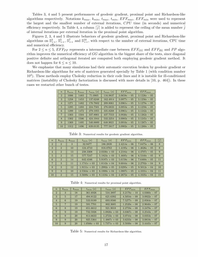
Tables 3, 4 and 5 present performances of geodesic gradient, proximal point and Richardson-likealgorithms respectively. Notations kmax, kmin, tmax, tmin, EFFmax, EFFmin were used to representthe largest and the smallest number of external iterations, CPU time (in seconds) and numericalefficiency respectively. In Table 4, a column dje is added to represent the ceiling of the mean number jof internal iterations per external iteration in the proximal point algorithm.
Figures 2, 3, 4 and 5 illustrate behaviors of geodesic gradient, proximal point and Richardson-likealgorithms on S3
++, S5++, S7
++ and S10++, with respect to the number of external iterations, CPU time
and numerical efficiency.For 2 ≤ n ≤ 5, EFFPP represents a intermediate case between EFFGG and EFFRL and PP algo-
rithm improves the numerical efficiency of GG algorithm in the biggest share of the tests, since diagonalpositive definite and orthogonal iterated are computed both employing geodesic gradient method. Itdoes not happen for 6 ≤ n ≤ 10.
We emphasize that many simulations had their automatic execution broken by geodesic gradient orRichardson-like algorithms for sets of matrices generated specially by Table 1 (with condition number104). These methods employ Cholesky reduction in their code lines and it is instable for ill-conditionedmatrices (instability of Cholesky factorization is discussed with more details in [10, p. 464]). In thesecases we restarted other bunch of testes.
n kmin kmax tmin (s) tmax (s) EFFmin EFFmax
2 1006 1483 71.0905 116.9837 3.0658e− 05 3.1226e− 05
3 1258 1453 137.6248 162.4914 3.0977e− 05 3.1256e− 05
4 1271 1482 176.7602 209.8061 3.0961e− 05 3.1278e− 05
5 1295 1493 224.7501 276.6833 3.0953e− 05 3.1259e− 05
6 1299 1472 279.1955 335.8208 3.0961e− 05 3.1242e− 05
7 1303 1504 337.8901 437.7553 3.0926e− 05 3.1262e− 05
8 1302 1506 424.1944 532.2254 3.0983e− 05 3.1245e− 05
9 1369 1495 540.8889 648.9021 3.0916e− 05 3.1267e− 05
10 1312 1496 639.0135 777.5817 3.0902e− 05 3.1260e− 05
Table 3: Numerical results for geodesic gradient algorithm.
n kmin kmax tmin (s) tmax (s) EFFmin EFFmax dje2 2 3 32.9477 186.2839 2.4214e− 06 7.8475e− 06 8
3 2 10 124.4710 816.0763 1.4195e− 06 1.4626e− 05 8
4 2 13 238.3308 2.0330e+ 03 4.2184e− 06 4.4707e− 05 9
5 2 15 577.7247 5.1823e+ 03 5.4695e− 06 6.5340e− 05 9
6 2 14 642.4346 5.9187e+ 03 5.6158e− 06 7.6468e− 05 11
7 3 11 1.1741e+ 03 1.8143e+ 04 9.6044e− 06 2.2792e− 04 9
8 3 12 1.9151e+ 03 1.2992e+ 05 2.0295e− 05 9.5012e− 04 10
9 3 10 2.5564e+ 03 6.1888e+ 04 1.0807e− 05 4.1031e− 04 11
10 2 15 3.5688e+ 03 8.1416e+ 04 2.2672e− 05 4.1635e− 04 15
Table 4: Numerical results for proximal point algorithm.
n kmin kmax tmin (s) tmax (s) EFFmin EFFmax
2 3 18 361.6926 534.3897 3.2176e− 10 4.0360e− 07
3 5 17 494.8122 621.6392 4.5054e− 09 3.0922e− 07
4 6 19 533.9189 693.9580 7.5277e− 09 2.8564e− 07
5 7 19 591.7701 802.3685 1.2520e− 08 2.9640e− 07
6 8 19 651.6612 921.9018 2.2759e− 08 3.2478e− 07
7 9 19 732.5926 1.0920e+ 03 3.0367e− 08 3.2543e− 07
8 9 20 814.6633 1.2723e+ 03 3.0744e− 08 3.0353e− 07
9 9 20 925.5364 1.4887e+ 03 3.6233e− 08 3.0818e− 07
10 9 20 1.0566e+ 03 1.7371e+ 03 3.5930e− 08 3.4445e− 07
Table 5: Numerical results for Richardson-like algorithm.
17

Figure 2: n = 3. Figure 3: n = 5.
Figure 4: n = 7. Figure 5: n = 10.
6.2 Conclusions
In this work, we present a feasible proximal point technique to compute the intrinsic Karcher meanof, n × n, SPD matrices under a strictly Riemannian look. Here, proximal point algorithm workscomputationally in two phases employing ideas similar to predictor-corrector methods. However, itdiffers from this class of methods because feasibility of diagonal positive definite and orthogonal stepsare held by Riemannian structures of Sn++, restricted to Dn++, and On respectively. Solutions forboth subproblems generated by our proximal point algorithm are approached employing the geodesicgradient algorithm with Armijo’s line search. Unfortunately, (Euclidean or geodesic) gradient methodsare not the best choice of algorithm to compute solutions of optimization problems because they spendexpensive number of external iterations to return approaches with hard accuracy (or they make tiny
18

step lengths near the optimum breaking its execution before to get the required accuracy). Other fastand efficient riemannian algorithms to solve both diagonal positive definite and orthogonal subproblemsare being investigated. We believe that it will improve the CPU time and numerical efficiency of ourmethod. Since elements of the proximal trajectory are defined as solutions of extended Moreu-Yosidaregularizations, whose structures are similar to original IKM problem, the methodology employed todetermine X(k+1) can be applied directly to solve it. Still, computational experiments may be made.Real applications, as Riemannian weighted mean of image data in [27], and other geodesic convexproblems on SPD matrices set will also be investigated under a proximal point view in the future. Inaddition, proximal point algorithm as presented here can be extended to other domains of positivitywhere Schur Theorem makes sense. According to [21, p. 189], the hermitian matrices set also representsan example of domain of positivity and spectral theorem is still held for it, where On is replaced byunitary matrices set Un. For instance, it justifies our conjecture.
Acknowledgements. This research was developed in cooperation with researchers from Departamentode Tecnologias e Linguagens of Universidade Federal Rural do Rio de Janeiro and Programa de Enge-nharia de Sistemas e Computacao of Universidade Federal do Rio de Janeiro and it has been supportedby FAPERJ as part of the research project intituled “Algoritmo de Ponto proximal em domıniosde positividade”, set in 2012, March. Authors thank Karine Gomes dos Santos Souza, a promi-sing computer science student from Departamento de Tecnologias e Linguagens, sponsored by FAPERJ,for partial development of Matlab code to proximal point algorithm and simulations, and FAPERJ forsupport.
References
[1] R. Bhatia, Positive definite matrices, Princeton Series in Applied Mathematics, Priceton UniversityPress, New Jersey, 2007.
[2] D. A. Bini, B. Iannanzo (2010), The matrix mean toolbox,<http://bezout.dm.unipi.it/software/mmtoolbox/> (retrieved 29.07.11).
[3] D. A. Bini, B. Iannazzo, Computing the Karcher mean of symmetric positive definite matrices,Linear Algebra and its Applications, 438 (2013), pp. 1700-1710.
[4] R. L. Bishop, B. O’Neill, Manifolds of negative curvature, Transactions of the American Mathe-matical Society, 145 (1969), pp. 1-49.
[5] C. A. Castano-moraga, C. Lenglet, R. Deriche, J. Ruiz-Alzola, A Riemannian approach toanisotropic filtering of tensor fields, Signal processing, 87 (2007), pp. 263-276.
[6] O. P. Ferreira, P. R. Oliveira, Proximal point algorithm on Riemannian manifolds, Optimization,51 (2002), pp. 257-270.
[7] S. Fiori, Quasi-geodesic neural learning algorithms over the orthogonal group: A tutorial, Journalof Machine Learning Research, 6 (2005), pp. 743-781.
[8] S. Fiori, Learning the Frechet mean over the manifold of symmetric positive-definite matrices,Journal of Cognitive Computation, 1 (2009), pp. 279-291.
[9] P. T. Fletcher, S. Joshi, Riemannian geometry for the statistical analysis on diffusion tensor data,Signal processing, 87 (2007), pp. 250-262.
[10] G. H. Golub, C. Van Loan, Matrix Computations, 3th edition, The Johns Hopkins University Press,Baltimore, Maryland, 1996.
19

[11] R. Gregorio, P. R. Oliveira, Proximal point algorithm with Schur decomposition on the cone ofsymmetric semidefinite positive matrices, Journal of Mathematical Analysis and Applications, 355(2009), pp. 469-479.
[12] R. A. Horn, C. R. Johnson, Matrix Analysis, 1st edition, Cambridge University Press, New York,1985.
[13] P. Kingsley, Introduction to diffusion tensor imaging mathematics: part III. Tensors calculation,noise, simulations and optimization, Concepts in magnetic resonance part A, 28A (2006), pp.155-179.
[14] C. Lenglet, M. Rousson, R. Deriche, O. Faugeras, Statistics on the manifold of multivariate normaldistribuitions: theory and application to diffusion tensor MRI processing, Journal of MathematicalImaging and Vision, 25 (2006), pp. 423-444.
[15] J. H. Manton, A globally convergent numerical algorithm for computing the centre of mass oncompact Lie groups, in Proceendings of the 8th International Conference Control, Automation,Robotics and Vision, 3, 2004, pp. 2211-2216.
[16] B. Martinet , Regularisation d’inequations variationnelles par approximations successives, RevueFrancaise d’Informatique et Recherche Operationelle, 4 (1970) , pp. 154-158.
[17] M. Moakher, A differential geometry approach to the geometric mean of symmetric positive-definitematrices, SIAM Journal on Matrix Analysis and Applications, 26 (2005), pp. 735-747.
[18] X. Pennec, P. Fillard, N. Ayache , A Riemannian framework for tensor computing, InternationalJournal of Computer Vision, 66 (2006), pp. 41-66.
[19] A. P. Papa Quiroz, P. R. Oliveira , Proximal Point Methods for Quasiconvex and Convex Functionswith Bregman Distances on Hadamard Manifolds, Journal of Convex Analysis, 16 (2009), pp. 49-69.
[20] R. T. Rockafellar, Monotone operators and the proximal point algorithm, SIAM Jounal on Controland Optimization, 14 (1976), pp. 877-898.
[21] O. S. Rothaus, Domains of positivity, Abhandlungen aus dem Mathematischen Seminar der Uni-versitat Hamburg, 24 (1960), pp. 189-235.
[22] T. Sakai, Riemannian geometry, Translations of mathematical monographs, 149, American Mathe-matical Society, Providence, RI, 1996.
[23] S. T. Smith Optimization techniques on Riemannian manifolds, in Hamiltonian and gradient flows,algorithms and control, Fields Intitute Communications, 3, American Mathematical Society, Prov-idence, RI, 1994, pp. 113-136.
[24] J. Stoer, R. Bulirsch, Introduction to numerical analysis, 3th edition, Springer-Verlag, New York,2010.
[25] C. Udriste, Convex functions and optimization methods on Riemannian manifolds, Mathematicsand Its Applications, Kluwer Academic Publishers, 297, The Netherlands, 1994.
[26] Y. Yang, Optimization on Riemannian manifolds, in Proceendings of the 38th conference on decision& control, Phoenix, Arizona, USA, 1999, pp. 888-893.
[27] F. Zhang, R. E. Hancock, New Riemannian techniques for directional and tensorial image data,Pattern recognition, 43 (2010), pp. 1590-1606.
20